Mergers of binary neutron stars with realistic spin
Abstract
Simulations of binary neutron stars have seen great advances in terms of physical detail and numerical quality. However, the spin of the neutron stars, one of the simplest global parameters of binaries, remains mostly unstudied. We present the first, fully nonlinear general relativistic dynamical evolutions of the last three orbits for constraint satisfying initial data of spinning neutron star binaries, with astrophysically realistic spins aligned and antialigned to the orbital angular momentum. The initial data are computed with the constant rotational velocity approach. The dynamics of the systems is analyzed in terms of gauge-invariant binding energy vs. orbital angular momentum curves. By comparing to a binary black hole configuration we can estimate the different tidal and spin contributions to the binding energy for the first time. First results on the gravitational wave forms are presented. The phase evolution during the orbital motion is significantly affected by spin-orbit interactions, leading to delayed or early mergers. Furthermore, a frequency shift in the main emission mode of the hyper massive neutron star is observed. Our results suggest that a detailed modeling of merger waveforms requires the inclusion of spin, even for the moderate magnitudes observed in binary neutron star systems.
pacs:
04.25.D-, 04.30.Db, 95.30.Sf, 95.30.Lz, 97.60.JdI Introduction
Neutron stars in binaries are spinning objects Lorimer (2008). The most famous example is the double pulsar PSR J0737-3039 for which the orbital period, both spin periods, as well as both spin down rates are known Lyne et al. (2004). The faster spinning pulsar in this system has a spin period of ms (PSR J0737-3039A) Burgay et al. (2003), which corresponds to a dimensionless spin of Tichy (2011); Damour et al. (2012a); Brown et al. (2012); Hannam et al. (2013). This is the fastest spinning pulsar in a binary system observed so far. From the orbital period we can estimate that this system will merge in about My due to emission of gravitational waves (GWs). Over this time period the faster spin will decrease by only about if we assume spin down is due to magnetic dipole radiation Tichy (2011). Thus we do expect spin effects near merger, even though the other spin is much smaller and plays no big role for this system.
A value of may appear rather small. For black hole systems is expected to approach in some cases. A theoretical limit for isolated neutron stars described by a large class of nuclear equations of state and uniform rotation is Lo and Lin (2011). Configurations with are however possible if, for example, differential rotation is allowed, e.g. Duez et al. (2004). It is not clear whether or how many of these large spin, single neutron stars can be found in binaries. Theoretical limits for neutron star in binaries depend on the mechanism of binary formation and binary history and are difficult to predict precisely Lorimer (2008). Given that the observed neutron star spin in binaries is comparatively small, star rotation is often ignored when modeling likely astrophysical neutron star mergers.
Binary neutron stars (BNS) are a primary source of GWs. Advanced interferometric configurations in LIGO and Virgo experiments are expected to detect from to events per year, starting from 2018-2019 (or even from 2016) Abadie et al. (2010); Aasi et al. (2013). At the expected sensitivities, neglecting spin effects in template-based searches of BNS can lead to substantial losses in the matched filter signal-to-noise ratio for the inspiral Ajith (2011); Brown et al. (2012). Template waveforms of the inspiral phase that cover most of the relevant frequency band are typically constructed with postNewtonian approximants. However, of particular interest is also the detection of the late-inspiral-merger waveforms, because such signals can be used to constrain the high-density equation of state (EOS) of neutron stars Read et al. (2009); Damour et al. (2012a); Del Pozzo et al. (2013). Differently from the inspiral case, precise merger waveforms can be constructed only by means of numerical relativity simulations, e.g. Baiotti et al. (2011); Bernuzzi et al. (2012a, b); Hotokezaka et al. (2013).
Although spin is one of the elementary parameters of a binary system, most studies of BNS to date have not considered neutron stars with realistic rotation. Almost all BNS simulations have started from initial data which have been constructed as (quasiequilibrium) stationary solutions in circular orbits, within either the corotational Baumgarte et al. (1997); Mathews et al. (1998); Marronetti et al. (1998) or the irrotational Bonazzola et al. (1999); Marronetti et al. (1999); Uryu and Eriguchi (2000); Taniguchi and Gourgoulhon (2002); Uryu et al. (2006, 2009) approach. There is spin in the corotational case, but it is determined by the orbital period and describes an unrealistic configuration because of the low viscosity of neutron star matter Bildsten and Cutler (1992).
Numerical simulations of BNS mergers in full general relativity have reached a high degree of precision and detail. Recent developments include radiation transport Sekiguchi et al. (2011a), microphysical equations of state Sekiguchi et al. (2011b), nonideal magnetohydrodynamics Palenzuela et al. (2013), as well as highly eccentric mergers Gold et al. (2012); East and Pretorius (2012). See Faber and Rasio (2012) for a review and more references. In all these simulations the Einstein equations are solved without any approximation as a 3+1 evolution system for a given initial configuration. Most BNS simulations have focused on irrotational configurations. In this case the stars’ spin is neglected, and not modeled in the simulations. A way to construct quasiequilibrium BNS initial data in circular orbits with spins has been recently proposed in Tichy (2011, 2012). The constant rotational velocity (CRV) formalism developed there is, to date, the only consistent method to produce realistic initial data for BNS mergers with spins (see Marronetti and Shapiro (2003); Baumgarte and Shapiro (2009) for earlier approximate approaches).
In this work we report dynamical evolutions of BNS initial data constructed with the CRV approach. We study the dynamics of the last three orbits, merger and postmerger phase, of equal-masses BNS configurations with spins aligned or antialigned to the orbital angular momentum. The rotational period of each star is moderate and compatible with astrophysical observations. We propose two simple ways to estimate the dimensionless spins of the binary and show that both agree within . The dynamics and gravitational radiation emitted are systematically compared with an irrotational configuration with the same rest mass. The orbital evolution is studied by means of gauge-invariant binding energy vs. orbital angular momentum curves Damour et al. (2012b). We compare these curves with a binary black hole simulation and with analytical models, show consistency of the results, and extract the different contributions to the binding energy from spin and tidal interactions. The merger remnant is also investigated, focusing in particular on the effect of rotation on the hypermassive neutron star.
Our results are the fundamental first step towards the use of CRV initial data for modeling rotating stars in BNS mergers. In particular, we show that even moderate spins have a significant impact on the merger dynamics and on the gravitational radiation emitted. Numerical relativity simulations aiming at an accurate description of the gravitational waves emitted by these sources should take into account the rotation of the star.
General relativistic evolutions of spinning neutron stars have been considered for a long time in the corotational approach, both in full general relativity and in the conformally flat approximation, see e.g. Shibata and Uryu (2000); Oechslin and Janka (2007) and Faber and Rasio (2012) for other references. More recently, alternative approaches have been proposed in Kastaun et al. (2013); Tsatsin and Marronetti (2013). Both works employ constraint-violating initial data produced by superposing either two boosted single-star configurations or an arbitrary velocity pattern. Such data violate both Einstein constraints and some hydrodynamical stationarity conditions. It is unclear how these initial data relate with the ones used in this work. Thus, in the following, we do not attempt a direct comparison of the results, but just point out certain similarities.
The paper is organized as follows. In Sec. II we review main aspects of the initial data and describe how to estimate the spin of our configurations. The numerical method is summarized in Sec. III. The dynamics of the numerical evolutions is analyzed in Sec. IV, by considering: (i) the analysis of the orbital motion with binding energy vs. orbital angular momentum curves; and (ii) the postmerger phase and a mode analysis of the hyper-massive neutron star in the merger remnant. Gravitational radiation is discussed in Sec. V. We conclude in Sec. VI.
Dimensionless units are employed hereafter, physical units are sometimes explicitly given in the text for clarity.
II Equilibrium configurations
| Name | ||||||||
|---|---|---|---|---|---|---|---|---|
| -0.00230 | 2.99932 | 8.69761 | 1.51496 | -0.11449 | -0.0499 | -0.10224 | -0.0419 | |
| -0.00115 | 2.99911 | 8.79949 | 1.51487 | -0.05710 | -0.0249 | -0.05130 | -0.0198 | |
| 0.00000 | 2.99903 | 8.90209 | 1.51484 | 0.00000 | 0.0000 | 0.00000 | 0.0000 | |
| 0.00115 | 2.99907 | 9.00585 | 1.51487 | 0.05710 | 0.0249 | 0.05188 | 0.0252 | |
| 0.00230 | 2.99926 | 9.11092 | 1.51496 | 0.11449 | 0.0499 | 0.10442 | 0.0480 | |
| -0.00460 | 3.00012 | 8.49472 | 1.51533 | -0.23128 | -0.1007 | -0.20368 | -0.0861 | |
| 0.00000 | 2.99903 | 8.90209 | 1.51484 | 0.00000 | 0.0000 | 0.00000 | 0.0000 | |
| 0.00460 | 2.99993 | 9.32688 | 1.51533 | 0.23128 | 0.1007 | 0.21240 | 0.0950 |
II.1 A review of the CRV approach
The initial data used here are constructed using the CRV method Tichy (2011, 2012). For this method we use the Wilson-Mathews approach Wilson and Mathews (1995); Wilson et al. (1996), which is also known as conformal thin sandwich formalism York (1999), for the metric variables together with certain assumptions. The first assumption is the existence of an approximate helical Killing vector , such that
| (1) |
We also assume similar equations for scalar matter quantities such as the specific enthalpy . However, the 4-velocity is treated differently and it is not assumed that vanishes. Instead we write
| (2) |
where and are the irrotational and rotational parts of the fluid velocity. We then assume that
| (3) |
so the time derivative of the irrotational piece of the fluid velocity vanishes in corotating coordinates. We also assume
| (4) |
and
| (5) |
which describe the fact that the rotational piece of the fluid velocity is constant along the world line of the star center. These latter two assumptions lead to the name constant rotational velocity method.
For the data considered here we set
| (6) |
where is the center of the star (defined as the point with the highest rest mass density) and where is an arbitrarily chosen angular velocity vector. In Tichy (2012) we have verified that this specific choice leads to only a negligible shear, so that we can avoid any substantial differential rotation.
II.2 Selected configurations
The initial configurations considered in this work are polytropes, , with , individual rest mass (or baryonic mass) and different rotational states. Table 1 summarizes the main properties of the models. The rotation state of each star is characterized by its angular velocity . For the simulations described here we have chosen to point along the -direction, with the values given in Tab. 1. If we use to define a spin period for each star, the different spinning configurations in Tab. 1 correspond to periods of , and ms. Notice, however, that these periods are not exactly the spin periods an observer at infinity would measure. As we show in Appendix A the spin periods observed at infinity are about 10% larger. The initial data employed in this work are selected from equilibrium sequences similar to those computed in Tichy (2012); some details are given in Appendix B.
The individual isolation masses of the irrotational model are , which is equivalent to the ADM mass of a TOV star with the same rest mass as the binary’s individual . All the binary models have about the same proper separation of ( km). The ADM masses differ by a maximum of . The CRV formalism Tichy (2011, 2012) allows us to construct single rotating star configurations by assuming that the approximate Killing vector is the timelike Killing vector . We have thus computed single star models with half the rest mass of the binary and the same . Each model is characterized by an ADM mass and an ADM angular momentum . For the nonrotating model of course and ; other values are reported in Tab. 1. We will make use of these values in the following sections. We define , and scale the time in the plots with this mass.
Additionally to these BNS configurations, we consider a nonspinning equal-masses binary black hole (BBH) run. The initial configuration is identical to the one in Tab. III of Walther et al. (2009) with an initial separation of and an eccentricity of .
II.3 Spin estimates
In the CRV approach the natural quantity describing the spinning motion is , however in the context of GWs it is convenient to consider “a spin”. Since the spin of a single star in a binary is not unambiguously defined in general relativity, we propose here two simple different ways of estimating the spin magnitude .
A simple method (which to our knowledge is new in this context) is to consider single stars in isolation with the same rest mass and the same , computed as described in Sec II.2. These stars have a well defined angular momentum . We then take the spin to be
| (7) |
and the dimensionless spin to be . These values are reported in Tab. 1.
A second estimate is given by comparing each spinning configuration with the irrotational one. From Tab. 1 we observe that the spin does not contribute significantly to the ADM masses. Assuming that the differences in the total angular momentum are due to the spins of the stars, we write
| (8) |
Dimensionless spin values are given then by . The results are stated in Tab. 1 and differ from the previous estimate by .
A precise value of the dimensionless spin is necessary to construct binding energy vs. orbital angular momentum curves. We will show that a nontrivial agreement with analytical results can be obtained using Eq. (7).
III Numerical method
| Name | ||||||
|---|---|---|---|---|---|---|
| L1 | 6 | 2 | 128 | 0.225 | 128 | 7.20 |
| L2 | 6 | 2 | 144 | 0.200 | 144 | 6.40 |
| M | 6 | 2 | 168 | 0.171 | 168 | 5.49 |
| H | 6 | 2 | 192 | 0.150 | 192 | 4.80 |
Simulations are performed with the BAM code Thierfelder et al. (2011a); Brügmann et al. (2008, 2004); Brügmann (1999). The Einstein equations are written in 3+1 BSSNOK form Nakamura et al. (1987); Shibata and Nakamura (1995); Baumgarte and Shapiro (1999). 1+log and gamma-driver conditions are employed for the evolutions of lapse and shift, respectively Bona et al. (1996); Alcubierre et al. (2003); van Meter et al. (2006); see Thierfelder et al. (2011b) for a study of gauge condition performance in handling gravitational collapse. General-relativistic hydrodynamics (GRHD) equations are solved in conservative form by defining Eulerian conservative variables from the rest-mass density , pressure , internal energy , and 3-velocity, . An equation of state closes the system. We consider evolutions with a -law EOS
| (9) |
with for most of the configurations. Some control runs with a polytropic EOS, thus forcing a barotropic evolution, have also been performed (see Tab. 1.)
The evolution algorithm is based on the method-of-lines with explicit 4th order Runge-Kutta time integrators. Finite differences (4th order stencils) are employed for the spatial derivatives of the metric. GRHD is solved by means of a high-resolution-shock-capturing method Thierfelder et al. (2011a) based on primitive reconstruction and the Local-Lax-Friedrichs (LLF) central scheme for the numerical fluxes. Primitive reconstruction is performed with the 5th order WENO scheme of Borges et al. (2008), which has been found to be important for long term accuracy Bernuzzi et al. (2012b, a). The numerical domain is made of a hierarchy of cell-centered nested Cartesian grids. The hierarchy consists of levels of refinement labeled by . A refinement level has one or more Cartesian grids with constant grid spacing and points per direction. The refinement factor is two such that . The grids are properly nested in that the coordinate extent of any grid at level , , is completely covered by the grids at level . Some of the mesh refinement levels can be dynamically moved and adapted during the time evolution according to the technique of “moving boxes”. The Berger-Oliger algorithm is employed for the time stepping Berger and Oliger (1984), though only on the inner levels. Interpolation in Berger-Oliger time stepping is performed at second order. A Courant-Friedrich-Lewy factor of is employed in all runs. We refer the reader to Thierfelder et al. (2011a); Brügmann et al. (2008) for more details.
The grid configurations considered in this work are reported in Tab. 2. Because we evolve equal-mass binaries, we use bitant symmetry (evolving only the half space ) without loss of generality. We experimentally found that the nonconservative mesh refinement in BAM can lead to rest mass violations during the postmerger phase (when mass crosses AMR boundaries), and in turn degrade the quality of the simulation in the long-term. In order to minimize this systematic source of error, the number of points in the moving levels is set equal to the nonmoving ones; see Appendix C for more details. This is different from what was done in previous BAM simulations, that instead mostly focused on the orbital phase, e.g. Thierfelder et al. (2011a).
Gravitational radiation is computed by means of the Weyl scalar Brügmann et al. (2008) on a coordinate sphere of radius . The scalar is projected onto spin weighted spherical harmonics to compute the multipoles . The metric multipoles are calculated by integrating the relation . We use a frequency-domain procedure with a low-frequency cutoff Reisswig and Pollney (2011). The signal is integrated from the very beginning of the simulation, in order to include also the initial burst of radiation related to the conformal flatness of the initial data. The radiated energy and angular momentum perpendicular to the orbital plane are calculated as
| (10) | ||||
| (11) |
with . In the calculation of the total angular momentum we also include the components, although their contribution is nonzero only in the postmerger phase and in practice negligible.
IV Dynamics
In this section we discuss the effect of the star’s rotation on the binary dynamics. We formally define the merger as the peak of the amplitude (Sec. V), but recall that the two stars come in contact well before (see e.g. discussion in Bernuzzi et al. (2012a) and below). First we describe the orbital phase, i.e. evolution up to merger, then we consider the postmerger phase.

IV.1 Orbital motion
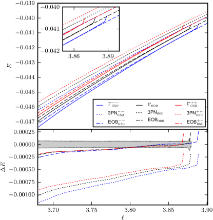
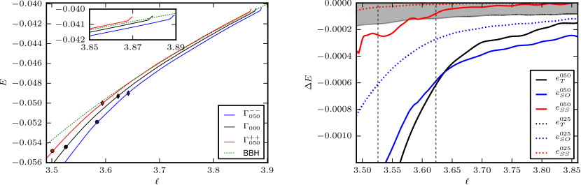
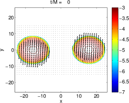
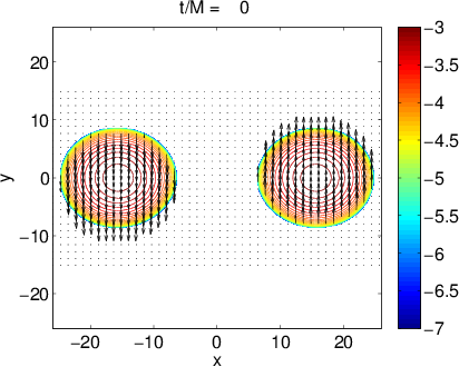
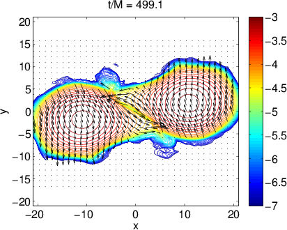
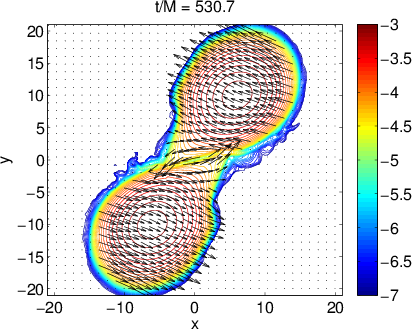
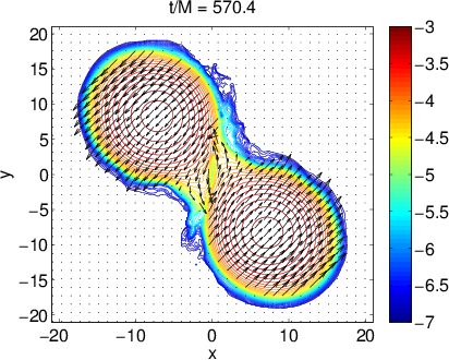
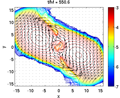
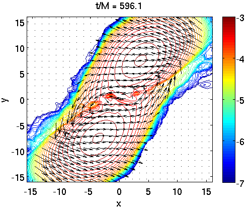
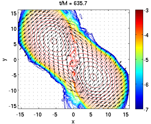
Figure 1 shows snapshots of the rest-mass density and fluid’s velocity on the orbital plane for the representative models , , and (columns). We focus on these since they are the -law EOS evolutions with the highest spin magnitudes. In the plot, the stars orbit each other counterclockwise. The top row refers to the initial time; comparing the central panel () with the left () and the right (), one can see only a very small difference in the velocity pattern due to the rotational state of the CRV data with respect to the irrotational flow. The central row refers to a simulation time at which the cores of the two stars come in contact, i.e. rest-mass density layers () of the two stars touch each other in the characteristic shearing contact, e.g. Sekiguchi et al. (2011a). The proper distance between the stars, as calculated from the local minima of the lapse function or local maxima of , is about at this moment. Note also the very different orbital phases of the three models at this moment, revealing that the moderate initial spins had a significant effect after only about orbits. The last row refers to the merger time, after approximately three orbits (six-seven GW cycles, see below), at which hyper massive neutron stars (HMNSs) are formed for the three configurations. The HMNSs appear similar in the snapshots, but their angular momentum is actually different and different dynamics follows (see Sec. IV.2.)
The orbital dynamics of the irrotational model is consistent with what was previously observed in e.g. Thierfelder et al. (2011a) for the same initial configuration computed with the Lorene code (see also Appendix C). The star rotation changes this picture: for spins aligned with the orbital angular momentum the inspiral is longer for larger spin magnitudes, while for antialigned spins the inspiral is shorter for larger spin magnitudes. This effect can be understood in term of spin-orbit interaction Damour (2001). Analogously to what happens to corotating/counter-rotating circular orbits in Kerr spacetimes, the last-stable-spherical orbit moves outwards (inwards) for antialigned (aligned) spin configurations with respect to the nonspinning case Damour (2001). The analogous result in binary black hole simulations is sometimes called “hang-up” Campanelli et al. (2006). In BNS mergers it has been discussed recently in Kastaun et al. (2013); Tsatsin and Marronetti (2013). Spin-orbit interactions thus change quantitatively the binary dynamics, and we quantify this aspect in the following.
A gauge invariant way to analyze the binary dynamics from numerical relativity data is to consider binding energy vs. orbital angular momentum curves, as proposed in Damour et al. (2012b). In the present context these curves allow us to characterize the dynamics generated by CRV initial data. We compute the dimensionless binding energy and angular momentum per reduced mass as 111 The notation for the angular momentum is slightly different from Damour et al. (2012b).
| (12) | ||||
| (13) |
respectively, where is the symmetric mass ratio, and the isolation mass is taken as , see Table 1. The initial angular momentum is computed from the spin estimates of Sec. II.3 as
| (14) |
and coincides with for the irrotational configuration. Eq. (13) assumes that only affects , i.e. the spin magnitude remains constant. This can be justified on a PN basis, and, in general, it holds for small, aligned spins.
| Name | ||||||||
|---|---|---|---|---|---|---|---|---|
| 499 | 0.067 | 3.64 | -4.89 | 551 | 0.124 | 3.58 | -5.19 | |
| 514 | 0.065 | 3.63 | -4.90 | 575 | 0.128 | 3.55 | -5.36 | |
| 531 | 0.069 | 3.62 | -4.92 | 595 | 0.127 | 3.53 | -5.44 | |
| 549 | 0.070 | 3.61 | -4.95 | 618 | 0.125 | 3.51 | -5.47 | |
| 570 | 0.071 | 3.60 | -4.99 | 636 | 0.123 | 3.50 | -5.48 |
The numerical data are compared to point-mass analytical results: a postNewtonian (PN) and an effective-one-body (EOB) Buonanno and Damour (1999, 2000) curve. In this work we employ the 3PN binding energy expression including next-to-next-to-leading order spin-orbit coupling as given by Eq. (43) of Nagar (2011), and indicate it as . The result rely on earlier achievements in PN theory, among others see Kidder et al. (1993); Kidder (1995); Tagoshi et al. (2001); Blanchet et al. (2004); Faye et al. (2006); Damour et al. (2008a); Steinhoff et al. (2008). Additionally, we also consider the curve constructed within the EOB approach in the adiabatic limit. For simplicity, we use the EOB model for spinning binaries introduced in Damour (2001). Similarly, the nonspinning part of the model is taken at 3PN accuracy Damour et al. (2000) only and it is resummed with a Padé approximant (see Barausse et al. (2012); Damour et al. (2013); Bini and Damour (2013); Pan et al. (2014) for recent theoretical developments of the EOB model.) The next-to-leading-order Damour et al. (2008b) and next-next-to-leading-order Nagar (2011) spin-orbit couplings are included in the Hamiltonian. We restrict ourselves to the leading order spin-spin term for simplicity, although the spin-spin interaction is known at next-to-leading order Balmelli and Jetzer (2013).
There is evidence that irrotational conformally flat initial data sequences are quite close to the 3PN result for a sufficiently large binary separation, e.g. Uryu et al. (2009) (and also Appendix B). However, we recall that the conformally flat approximation introduces errors already at 2PN level Damour et al. (2000). On the other hand, the 3PN-EOB adiabatic curve has been found to correctly reproduce nonspinning numerical relativity data of different mass ratios up to Damour et al. (2012b). The same reference has shown that the 3PN-EOB curve is instead remarkably close to numerical data up to the last stable orbit of the EOB potential (), and it is an accurate diagnostic of the conservative dynamics of the system. (See Bernuzzi et al. (2012b) for the case of neutron star mergers with irrotational data.)
The curves at early simulation times are shown in Fig. 2 for models , , and , together with the PN and EOB curves computed with the spin values as estimated in Sec. II.3. These curves are quite sensitive to small variations in the values of the initial masses, angular momentum and spins. For example, they require and accurate up to four digits. The uncertainty on the numerical data is also shown. It is estimated considering data at different resolutions (grid configurations H and L2) and including the uncertainty of the initial ADM values as measured from different SGRID resolutions. Both errors are added in quadrature. The bottom panel shows the differences of numerical data with respect to the 3PN and the EOB curves with the relative spin values.
We experimentally observe that, for all the configurations considered in this work, the spin estimate in Eq. (7) leads to curves closer to the PN and EOB ones at early times than Eq. (8). Thus, we use in the figure and in the following that estimate. Note that this choice assumes that the spin is almost constant along the sequences.
As shown in Fig. 2, the dynamics starts between the PN and EOB curves, and rapidly depart from the initial state, (see inset). This variation is due to the emission of the artificial gravitational radiation related to the conformally flat assumption of the CRV data. In complete analogy with the nonspinning binary black hole case and irrotational case, the numerical evolution settles very quickly close to the EOB curve (with the proper spin) Damour et al. (2012b); Bernuzzi et al. (2012b). The difference between the EOB curves and the numerical data at early times is within the error-bars: the tidal contribution cannot be distinguished with present data (the same happens comparing BNS and BBH, see below).
A clear hierarchy among the PN and EOB curves with different spins can be observed. This effect is due to spin-orbit interactions: antialigned configuration are more bound and aligned configurations are less bound than irrotational (cf. “hang-up”). The numerical curves consistently respect such hierarchy from early times to merger (see below). During the early-times evolution, the binaries binding energies depart systematically from the EOB, and close to contact (), the deviation becomes significant. Note in the bottom panel how the differences between EOB and numerical data for different spins are essentially indistinguishable. This fact clearly suggests that the deviation is due to finite size effects.
The curves up to merger are shown in Fig. 3 (left panel) for models , , and together with the one for the nonspinning BBH run. At early times (see inset) the BBH system is less bound than the irrotational configuration, but within the data uncertainty. As observed for the EOB curve, for tidal contributions become progressively more important and the systems become more bound deviating systematically from the BBH curve. Merger occurs at , , for , and , respectively. At merger, the aligned spin configurations are more bound than the antialigned one. See also Tab. 3 for a collection of relevant numbers for all the configurations.
In order to gain insight into the role of spin and tidal interactions during the merger phase, we make the assumption that
| (15) |
i.e. that the binding energy of a spinning BNS configuration can be approximated by the sum of four separate contributions: a nonspinning point-mass (black-hole) term , a spin-orbit (SO) term , spin-spin (SS) term , and a tidal (T) term . The different terms have PN contributions starting from 1.5PN (SO), 2PN (SS) and 5PN (T). All the four terms in (15) can be calculated using the simulation data, e.g. the four runs , , , and BBH. Below we distinguish between the terms in the ansatz () and the numerical curves (, as the relative model name). The SO term has structure of the form , so for aligned/antialigned spins . Similarly, the SS term has structure , so it does not change sign if both spins flip. A binary configuration has a repulsive SO contribution (), whereas a one with the same spin magnitude has an attractive SO contribution () to the binding energy. However, as mentioned above, the aligned spin configurations give a more negative binding energy at merger than the antialigned configurations (compare with Damour (2001).)
The SO term is calculated by the combination of the aligned/antialigned spins runs with the same magnitude, i.e. . Obviously we pose and , and calculate from the difference . The SS term is estimated as . The different terms are reported in the right panel of Fig. 3. The SS contribution is the smallest negative, at the level of the uncertainty of the data. At the moderate spins used here, SS interactions are essentially not resolved in the simulation. On the other hand, the curves and are well resolved. We observe that, for , the is the dominant contribution to the binding energy up to . After this point, becomes dominant. This corresponds to intuition since the dynamics reaches the hydrodynamical regime (see Fig. 1). Towards merger (not visible in the plot) the differences between the and become progressively larger.
An independent estimate of , , and is also given by using the data of the other two simulations , see right panel of Fig. 3. We obtain similar results, and in particular the terms exactly coincide as they should. There is one important difference though. In the case , the term is the largest negative term already at early simulation times. Thus during the last three orbits the binding energy is “tidally dominated” as in the irrotational case.
We mention that, while the SS term is poorly resolved, its presence is clearly suggested by looking at the difference and . The two combinations approximate , with the SS term entering with a different sign. We find that, as expected, the former is less bound, the latter is more by a small amount. Similarly, inspection of the quantity , leads to a curve very close to , only slightly more bound. This suggests that there is no significant coupling between SO and tidal contributions (as assumed in Eq. (15)), even after contact.
Finally, note that for the spin term is probably influenced by hydrodynamical effects, so its correct interpretation may be nontrivial. We also mention that similar results and conclusions are obtained by using the EOB curves instead of the BBH data.
IV.2 Merger remnant
All the configurations evolved with the -law EOS form, at merger, HMNSs characterized by different rotational states. In our simulations the HMNS is only supported by centrifugal forces and thermal pressure (we include neither magnetic fields nor cooling mechanisms). The angular momentum support is radiated away in GWs on dynamical timescales, and the HMNS finally collapses. This happens after about M ( ms) from formation in the irrotational model. The dimensionless angular momentum magnitude per reduced mass of the HMNS is approximately (assuming ), e.g. , , for , , and , respectively. We thus expect that configurations with antialigned spins will collapse earlier, whereas configurations with aligned spins will collapse later.
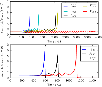
In Fig. 4 we show the evolution of the maximum rest mass density, , for evolutions with the -law EOS (upper panel) and the polytropic EOS (lower panel). The oscillations visible in the plot correspond to quasiradial modes (see below and Sec. V). The average rest mass density increases linearly in time to about a critical density, ( ), at which collapse happens. As expected, we observe that model collapses after approximately two quasiradial oscillations, model after five, and model after twelve. Model survives for several dynamical timescales and does not collapse until the end of the simulation ( M.) We have not evolved further since (i) long-term simulations can become inaccurate (see Appendix C), and (ii) on these timescales other physical effects like magnetic fields and neutrino cooling, presently not included, play an important role, e.g. Sekiguchi et al. (2011b); Paschalidis et al. (2012); Hotokezaka et al. (2013); Deaton et al. (2013). However, considering a linear trend in , we extrapolate that collapse should happen at about M ( ms) after merger.
The lower panel of Fig. 4 refers to configurations evolved with a polytropic EOS. Since in this case thermal pressure support is absent, collapse occurs much earlier than for the -law EOS. The HMNS of the irrotational configuration collapses after about one quasiradial oscillation; model promptly collapses without HMNS formation, and model collapses after few oscillations.
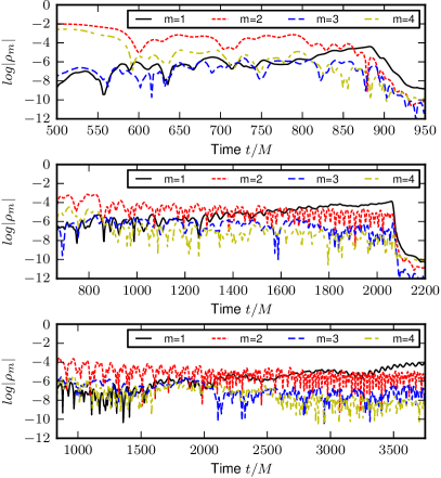
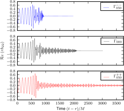
During its evolution the HMNS oscillates nonlinearly and becomes progressively more compact. The oscillations modes can be identified as the quasiradial mode, the -mode, and nonlinear combinations of them, e.g. Shibata and Uryu (2000); Stergioulas et al. (2011). A way to characterize nonlinear modes is to project the rest-mass density onto spherical harmonics, e.g. Baiotti et al. (2009a). For simplicity, we consider in the orbital plane and the projections Stergioulas et al. (2011)
| (16) |
In Fig. 5 we report the evolution of the first projections for some representative runs. The figure shows that the dominant mode is the mode. Actually, the projection/mode with larger amplitude is the quasiradial one (, also visible in Fig. 4). As we shall discuss later, however, this mode has a frequency too low to be visible in the GW spectrum. The evolution of is qualitatively similar in the different configurations, with differences only related to the collapse time. A strong mode appears in all simulations before collapse (see e.g. the central panel) and also dominates the evolution of after M. We interpret it as a physical hydrodynamical effect due to mode couplings, but we cannot rule out that it is triggered by some numerical effect.
| 584 (34) | 1543 (38) | 2974 (114) | |
| 594 (34) | 1482 (38) | 2871 (103) | |
| 671 (13) | 1341 (13) | 2738 (76) |
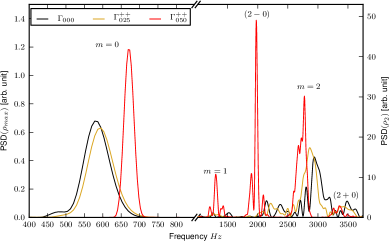
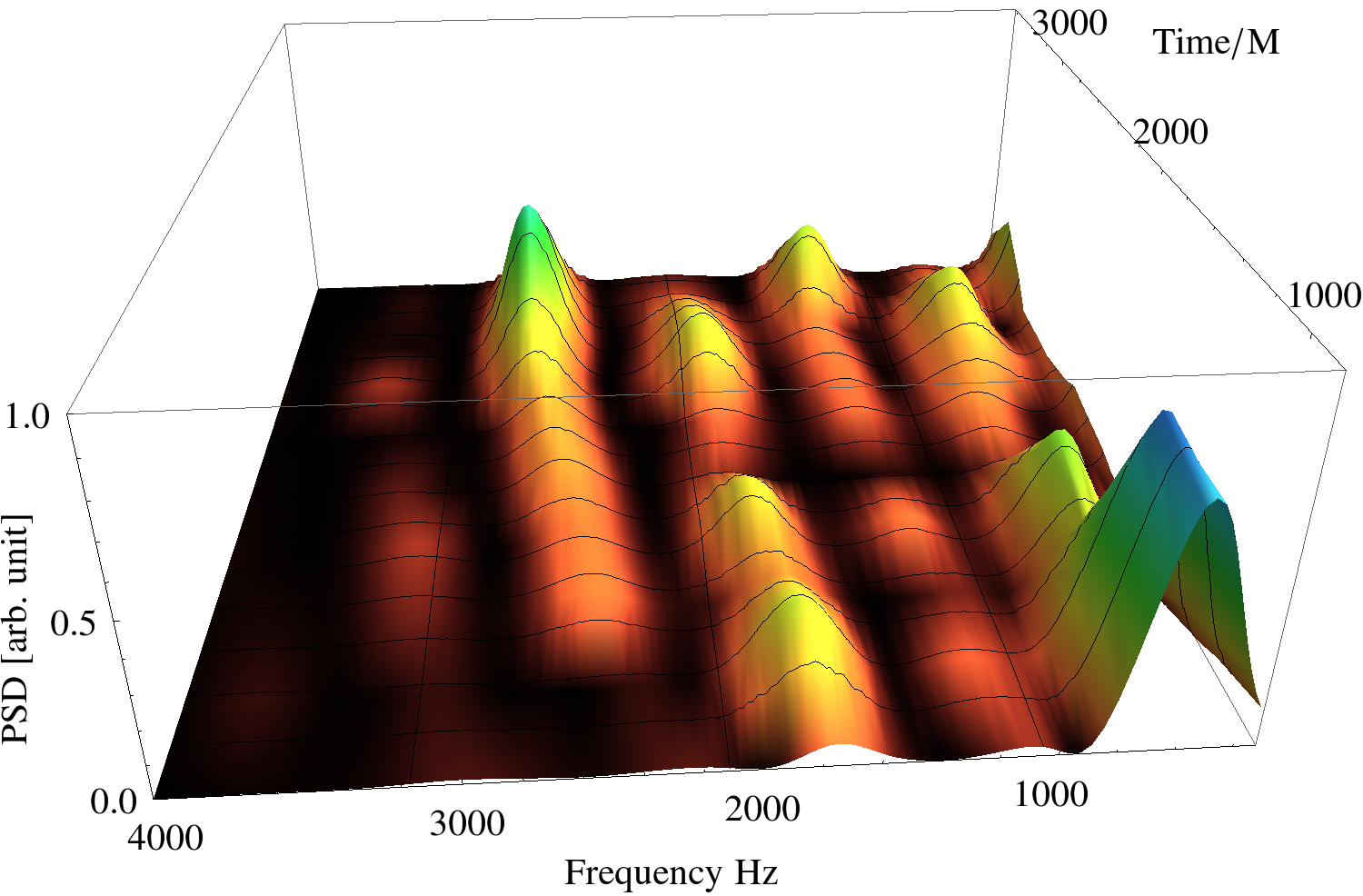
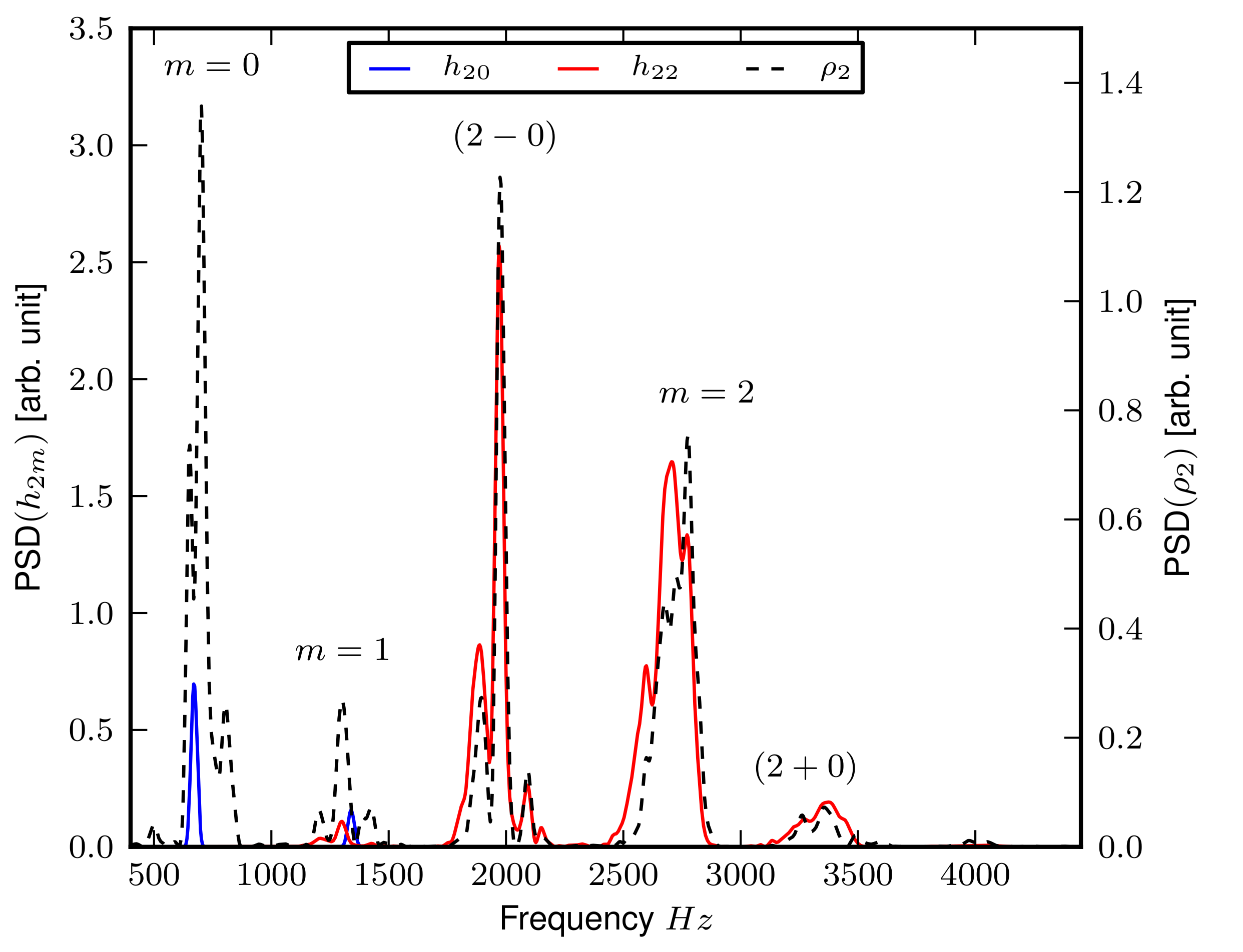
In order to extract the mode frequencies, we perform a Fourier analysis of the projections and . The quasiradial mode is best extracted from the latter. The Fourier transform is performed only in the part of the signal after merger, i.e. . Some of the relevant results are summarized in Fig. 6, where we show on the left the spectra of for lower frequencies and for higher frequencies for different models and on the right the spectrogram of model . Focusing on the left panel, we observe that the spectrum is composed of few frequencies; we identify modes together with nonlinear couplings “” Stergioulas et al. (2011); Dimmelmeier et al. (2006); Baiotti et al. (2009a). For model the highest power is actually found at the “2-0” frequency in .
The peak frequencies for the different modes and models are stated in Tab. 4 for the relevant case of spin aligned with the orbital angular momentum. The frequency peak of the mode becomes larger the smaller the HMNS rotation is. This is because the HMNS with more angular momentum support is less compact, and the proper frequencies decrease if the compactness decreases (compare with sequences of a single rotating star with the same rest mass in Dimmelmeier et al. (2006)). Notably, for model the observed frequency shift with respect to the irrotational configuration is 236 Hz. The value is significant at the - level, see Tab. 4. Differently from the mode, the frequency of the quasiradial mode () is found to increase for HMNS with larger angular momentum. As discussed in Stergioulas et al. (2011), the quasiradial mode frequency depends on the compactness of the HMNS and on how close the star model is to the collapse-instability threshold. The larger the compactness, the larger the mode frequency is; but configurations close to the instability threshold can have smaller frequencies since the instability threshold is a neutral point. We interpret our results according to the above argument: HMNSs with larger angular momentum support are further from collapse threshold and thus have higher frequencies.
The spectra lines appear broad due to the highly dynamical nature of the HMNS. Investigating the dynamical excitation of the modes by a spectrogram, we find that (i) the modes are “instantaneously” characterized by relatively narrow peaks; (ii) different modes dominate different parts of the signal; (iii) some of the peaks “drift” towards higher frequencies as the HMNS becomes more compact. The right panel of Fig. 6 shows the spectrogram of the quantity for . At early times the (quasiradial) mode dominates the spectrum, but around M the becomes the main oscillation mode. A “drift” of the mode towards higher frequencies is visible, which corresponds to the fact that the HMNS becomes more compact. The “2-0” coupling remains the secondary peak during the whole simulation. The and “2+0” modes are also visible. At the very end of the evolution the mode has the largest power.
| P | P000 | P | |||||
|---|---|---|---|---|---|---|---|
| 2.92 | 2.88 | 2.85 | 2.86 | 2.95 | 2.94 | 2.89 | |
| 0.80 | 0.79 | 0.78 | 0.79 | 0.81 | 0.83 | 0.84 | |
| 0.039 | 0.068 | 0.081 | 0.082 | 0.006 | 0.021 | 0.065 | |
| 1.2% | 2.1% | 2.5% | 2.5% | 0.2% | 0.6% | 2.0% |
Finally, we briefly discuss the black hole and the remnant disk. All simulations (except ) result in a black hole surrounded by a nonmassive accretion disk. Tab. 5 summarizes the irreducible mass and the dimensionless spin of the black hole, and the rest mass of the disk. The black hole mass is larger for antialigned spin configurations and spin magnitude, and a monotonic trend is observed for smaller spin and aligned spin configurations. The opposite holds for the disk mass. The spin of the black hole is larger for aligned configurations in barotropic evolutions. This effect is not visible in the -law simulations, in which the more massive disk probably has also larger angular momentum. The maximum spin produced is , which is consistent with the upper limit found in Kastaun et al. (2013). Notice that all reported quantities are affected by large uncertainties, and they should be considered only as a qualitative indication. For example the uncertainty on the black hole mass calculated from and runs of the irrotational configuration is .
V Gravitational radiation
The dynamics described in Sec. IV is relatively simple (but far from trivial). For sufficiently high spin magnitudes, , the SO interaction is a significant repulsive (attractive) contribution for aligned (antialigned) spins configurations. For aligned configuration the SO competes with finite size effects. At merger, however, binaries with aligned spins are more bound. HMNSs are formed with more or less angular momentum support than in the irrotational configuration (); thus they are either closer or farther from the collapse threshold (radial instability point). We discuss in this section how the emitted gravitational radiation encodes all this.
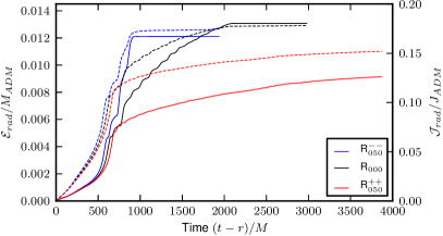
The total energy and angular momentum emitted in GWs quite differ in the different models, as can be seen from Fig. 7. The irrotational configuration emits about of the initial ADM mass and of the initial angular momentum. emits about the same amount, but in about half the time. To the end of the simulation, has emitted of the initial mass and about of the initial angular momentum. In all the cases, the main emission channel is the multipole that alone accounts for of the emitted energy. However, in the postmerger phase other channels are clearly excited; the largest amplitudes are observed in the , , the , , and the modes (in that order).
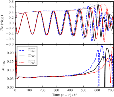
Figure 8 (left panel) shows the inspiral waveforms, focusing again on the models , and for clarity. Intermediate results are of course found for the other models. The upper-left panel shows the real part and amplitude of the mode of the GWs, the lower-left panel the GW frequency ; note the retarded time in the -axis. The merger times, computed at the peak of , are for , and , respectively (see also Tab. 3). The peaks of the wave amplitude are all very close to . The GW frequency corresponding to the peak of the wave amplitude is smallest for aligned spin. At merger for , , and , respectively. At contact instead . Note that these frequencies have uncertainties of about . The effect of spin-orbit interaction is clearly visible from the plot. Computing the accumulated phase of the GW, we find that the irrotational configuration emits 7.0 GW cycles to merger; emits 6.3 cycles and emits 7.3 cycles. This phase difference results from the dynamics discussed in Sec. IV.1, and encodes the interplay of spins and tidal interactions.
Let us finally discuss the emission from the HMNS. Figure 8 (right panel) shows the complete waveform. The earlier the HMNS collapses, the larger the amplitude of the wave in the postmerger phase is. As also shown in Fig. 7, model emits more energy and angular momentum than and during the first M after merger. In order to identify the origin of the emission, we perform a Fourier analysis of the and multipoles, and compare this with the mode analysis of Sec. IV.2. As in the previous section, we consider only the signal at . A relevant example of this analysis is summarized in Fig. 9. The spectra of the waves and matter modes strongly correlate: the HMNS modes are the main emitters during the postmerger phase Stergioulas et al. (2011). We stress that the complete GW spectrum includes also the inspiral part of the GW signal. In particular, the merger happens at GW frequencies of kHz, and, up to these frequencies, the spectrum is dominated by the inspiral. Thus the quasiradial mode frequency of the HMNS is not observable, whereas the and “” peaks form the main postmerger signal.
In Oechslin and Janka (2007); Bauswein and Janka (2012) (see also Hotokezaka et al. (2013)) it is shown that the frequency of the peak of the GW (postmerger) spectrum is strongly dependent on the EOS, and, to a lesser extent, on the total mass, mass ratio and spin. The latter aspect has been investigated by comparing irrotational and corotational configurations for a few models, and no significant frequency shift was observed. The long wave train of model allows us to resolve a significant frequency shift, suggesting that spin effects may be more important than previously thought. Note that a shift towards lower frequencies can favor GW detection by advanced interferometers.
VI Conclusion
We have studied BNS mergers in numerical relativity with a realistic prescription for the spin. Consistent initial data have been produced with the CRV approach and evolved for the first time.
We have considered moderate star rotations corresponding to dimensionless spin magnitudes of , and direction aligned or antialigned with the orbital angular momentum. The dimensionless spins are estimated by considering the angular momentum and masses of stars in isolation with the same rotational state as in the binary. We have investigated the orbital dynamics of the system by means of gauge invariant curves Damour et al. (2012b).
Our simple proposal for the estimation of proved to be robust, and allows us to show consistency with PN and EOB energy curves at early-times. Using energy curves we have also compared, for the first time to our knowledge, BNS and BBH dynamics (see Foucart et al. (2013) for a waveform-based comparison of the case BBH–mixed binary.) We extracted and isolated different contributions to the binding energy, namely the point-mass nonspinning leading term, the spin-orbit and spin-spin terms and the tidal term. The analysis indicates that the spin-orbit contribution to the binding energy dominates over tidal contributions up to contact (GW frequencies ) for . The spin-spin term, on the other hand, is so small that it is not well resolved in the simulations. No significant couplings between tidal and spin-orbit terms are found, even at a stage in which the simulation is in the hydrodynamical regime (at this point, however, the interpretation of “spin-orbit” probably breaks down.)
The spin-orbit interactions significantly change the GW signal emitted. During the three orbit evolution we observe an accumulated phase differences up to GW cycles (over three orbits) between the irrotation configuration and the spinning ones (), that is we obtain first quantitative results for orbital “hang-up” and “speed-up” effects. A precise modeling of the late-inspiral-merger waveforms, as in Bernuzzi et al. (2012b), needs to include spin effects even for moderate magnitudes. Long-term (several orbits) simulations are planned for a thorough investigation of this aspect, together with detailed waveform phasing analysis and comparison with analytical models. Extensive simulations with different EOSs will be also important to check the universal relations recently proposed in Bernuzzi et al. (2014).
We have also investigated spin effects on the formation and collapse of the merger remnants (HMNSs), and the hydrodynamical evolution the HMNS modes Stergioulas et al. (2011). The star rotation influences the HMNS produced at merger by augmenting (aligned spin configuration) or reducing (antialigned) the angular momentum support. Earlier or delayed collapse of several milliseconds is thus observed depending on the spins orientation. We have found that characteristic frequencies of the HMNS are shifted to lower values by rotation. This suggest that spin effects may be more important than previously thought. HMNS modes are the main emitters of GWs in the postmerger phase, and they may allow for a precise determination of the neutron star radius in a GW detection Bauswein and Janka (2012). Extensive evolutions of CRV configurations for various EOSs and spins are needed in order to assess the role of spin and to obtain accurate phenomenological relations for frequency vs. radius.
Future work should also be devoted to understanding the impact of our result on GW astronomy. We expect that some aspects of spin in BNS can be modeled similarly to the GW analysis for nonprecessing spinning BBHs Ajith et al. (2011); Hannam et al. (2010); Santamaria et al. (2010); Hannam et al. (2008). Furthermore, it would be important to explore the relevance of spin-orbit corrections in the construction of templates for detecting the star’s EOS Damour et al. (2012a); Favata (2014), possibly applying realistic data analysis settings Del Pozzo et al. (2013). In the relevant case of aligned spin configurations, spin-orbit effects actually compete with finite size effects. One might expect that, for some realistic spin magnitudes, this could affect the measurability of the EOS (tidal polarizability parameters) when spin is not properly taken into account. Similarly, if the spin is estimated from the early inspiral, a bias in the spin magnitude could significantly affect the measure of the tidal parameters Damour et al. (2012a).
Acknowledgements.
It is a pleasure to thank Alessandro Nagar for valuable comments and interactions, and Simone Balmelli for providing us with the EOB curves. We are also grateful to Nathan Kieran Johnson-McDaniel and Andreas Weyhausen for interesting discussions. This work was supported in part by DFG Grant SFB/Transregio 7 “Gravitational Wave Astronomy”, the Graduierten-Akademie Jena, and NSF Grants PHY-1204334 and PHY-1305387. Simulations were performed on SuperMUC (LRZ) and JUROPA (JSC).Appendix A Single spinning stars
In the CRV approach one assumes the existence of an approximate helical Killing vector. In an inertial frame it has the form Tichy (2012)
| (17) |
Here denotes the center of mass position of the system, and is the orbital angular velocity, which we have chosen to lie along the -direction.
For a single star coincides with the star center . Furthermore if we follow the CRV approach , since a single star is not orbiting. Thus the approximate Killing vector simply points along the time direction. We can then set the in Eq. (6) to the same value as in the case of binary stars. If we now solve the CRV equations we obtain initial data for a single spinning star. This spin can be unambiguously computed from the ADM angular momentum and reported in the column of Tab. 1.
However, there is at least one other way to obtain single spinning stars. We can set to a nonzero value and assume that the approximate Killing vector is truly helical. If we then assume that the fluid velocity is along the Killing vector
| (18) |
we obtain the standard assumptions for a corotating configuration, but for a single star only. If we now solve the usual equations for the corotating case (see e.g. Tichy (2009a)), we also obtain initial data for a single spinning star. Notice however, that the star spin in this corotating approach is about 10% higher than in the CRV approach if we set . This means that and do not have the same meaning, which is not too surprising considering that is just an auxiliary local field in the CRV construction, while is the angular velocity seen by observers at infinity.
The above observations can be used to estimate the angular velocity seen by observers at infinity when using the CRV approach for single stars. We first construct a single star using the CRV approach for a particular and compute its spin . We then choose such that the corotating approach results in the same spin. We can then interpret this as the angular velocity seen by observers at infinity for a single star with spin . If we follow these steps for e.g. , we find that we have to choose to obtain the same spin with the corotating approach. Thus the angular velocity seen at infinity for is really only , which makes sense considering that any local frequency will be redshifted by the time it is observed at infinity. Thus the spin period observed at infinity is about 10% larger than what we get from .
Appendix B Equilibrium sequences
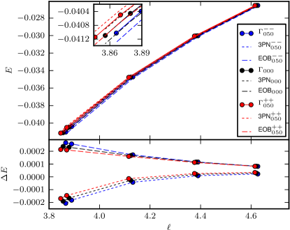
In this appendix we present the equilibrium sequences of CRV data, considering in particular the curves , where and ; see also Eq. (12) and (13). The numerical data are again compared to PN and EOB Buonanno and Damour (1999) results, as described in the main text.
In Fig. 10 we report the curves for sequences with . The 3PN and adiabatic EOB curve are very close to the data for large separations. The differences are quantified in the right panel, by plotting with 3PN, EOB. For the closest separation computed, the sequences equally deviate from EOB and 3PN curves, but while the 3PN result predicts a less bound binary, the EOB method predicts a more bound one. Note also a systematic difference in for different spins.
Appendix C Robustness of simulations in the postmerger phase
The accuracy of the simulations in the orbital phase has been studied in different recent works. In particular Refs. Thierfelder et al. (2011a); Bernuzzi et al. (2012a) presented the first convergence tests of waveform’s phase and amplitude in three and nine-to-ten orbits inspirals. We do not repeat that analysis here. The same works pointed out that after merger convergence cannot be monitored in the waveforms, and, in general, the results are much more dependent on the resolution and grid setup employed. See also Baiotti et al. (2009b) for similar conclusions obtained with other codes. In this appendix we discuss the robustness of the simulations in the postmerger phase, in particular regarding the merger remnant, i.e. HMNS. We consider two different series of tests: (i) an internal test based on a resolution study and different grid setup, and (ii) an external test that compares the same evolution of similar initial data obtained with SGRID and Lorene. We focus on the irrotational configuration.
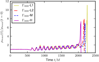
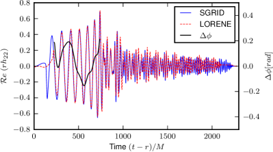
Fig. 11 shows the evolution of the maximum rest-mass density on the finest refinement level for the different resolutions considered in this work (see Tab. 2). The results show a converging behavior of this quantity with increasing resolution, making us confident that the chosen setup gives, at least qualitatively, correct results. As observed in previous works, it is impossible to prove strict convergence either in this quantity or in the waveforms.
Extensive tests in an early stage of the work have shown that the nonconservative mesh-refinement of BAM is not optimal for long-term evolution of the HMNS. During the inspiral the compact stars are contained and completely resolved in a single Cartesian box at the finest refinement level. In the postmerger phase, however, a significant amount of matter can cross grid boundaries, unsurprisingly leading to severe violations of the rest mass conservation. Only when the inner box encloses most matter, we expect systematic convergence.
As an example we consider the grid configuration L2 and an equivalent configuration in which the number of points in the moving levels are reduced from to (but the same resolution is used). With smaller boxes the outer layer of the HMNS are not covered by the finest refinement level. The larger mass violation of the setup with led to earlier (in this case study) black hole formation by about M. Note however that the rest mass is conserved for the L2 grid up to to collapse, while for the H grid up to .
In a second series of tests, we compare the evolutions obtained with the SGRID initial data with Lorene data Eric Gourgoulhon, Philippe Grandclément, Jean-Alain Marck, Jérôme Novak and Keisuke Taniguchi . The Lorene data considered here have been employed in several works in the past, e.g. Baiotti et al. (2009b); Thierfelder et al. (2011a). The initial separation slightly differs in the two cases: the proper distance is M for SGRID data and M for Lorene data. Lorene data employ four domains and the number of collocation points for each domain is . SGRID uses 4 compactified domains with points and 2 Cartesian domains with . The grid configuration used for the evolution in BAM is H.
Figure 12 shows the waveforms aligned before merger on the time window (support of the black line.) The waveforms are very similar; phase differences (black line) are below rad. This uncertainty is of the same order magnitude of a conservative error bar estimated from convergence tests. On the other hand, the HMNSs collapse within M ( ms) of each other.
We conclude that the results consistently approach a continuum limit when smaller grid spacings and sufficiently large boxes are employed. Results from different initial data are also consistent. However, care should be taken considering HMNS simulations of several milliseconds since relatively small mass violations can lead to quantitatively different behaviors. We have tested different grid setups, grid resolutions, and independent initial data (when possible). Based on these results we expect an uncertainty on the HMNS lifetime up to a maximum of 300M, which is considerably shorter than the difference between model and . Although not commonly used in numerical relativity, a conservative AMR Berger and Colella (1989) is desirable; see East et al. (2012); Reisswig et al. (2013) for the first recent applications in the field.
References
- Lorimer (2008) D. R. Lorimer, Living Rev. Rel. 11, 8 (2008), eprint 0811.0762.
- Lyne et al. (2004) A. Lyne, M. Burgay, M. Kramer, A. Possenti, R. Manchester, et al., Science 303, 1153 (2004), eprint astro-ph/0401086.
- Burgay et al. (2003) M. Burgay, N. D’Amico, A. Possenti, R. Manchester, A. Lyne, et al., Nature 426, 531 (2003), eprint astro-ph/0312071.
- Tichy (2011) W. Tichy, Phys.Rev. D84, 024041 (2011), eprint 1107.1440.
- Damour et al. (2012a) T. Damour, A. Nagar, and L. Villain, Phys.Rev. D85, 123007 (2012a), eprint 1203.4352.
- Brown et al. (2012) D. A. Brown, I. Harry, A. Lundgren, and A. H. Nitz, Phys.Rev. D86, 084017 (2012), eprint 1207.6406.
- Hannam et al. (2013) M. Hannam, D. A. Brown, S. Fairhurst, C. L. Fryer, and I. W. Harry, Astrophys.J. 766, L14 (2013), eprint 1301.5616.
- Lo and Lin (2011) K.-W. Lo and L.-M. Lin, Astrophys.J. 728, 12 (2011), eprint 1011.3563.
- Duez et al. (2004) M. D. Duez, Y. T. Liu, S. L. Shapiro, and B. C. Stephens, Phys.Rev. D69, 104030 (2004), eprint astro-ph/0402502.
- Abadie et al. (2010) J. Abadie et al. (LIGO Scientific Collaboration, Virgo Collaboration), Class.Quant.Grav. 27, 173001 (2010), eprint 1003.2480.
- Aasi et al. (2013) J. Aasi et al. (LIGO Scientific Collaboration, Virgo Collaboration) (2013), eprint 1304.0670.
- Ajith (2011) P. Ajith, Phys.Rev. D84, 084037 (2011), eprint 1107.1267.
- Read et al. (2009) J. S. Read, C. Markakis, M. Shibata, K. Uryu, J. D. Creighton, et al., Phys.Rev. D79, 124033 (2009), eprint 0901.3258.
- Del Pozzo et al. (2013) W. Del Pozzo, T. G. F. Li, M. Agathos, C. V. D. Broeck, and S. Vitale, Phys. Rev. Lett. 111, 071101 (2013), eprint 1307.8338.
- Baiotti et al. (2011) L. Baiotti, T. Damour, B. Giacomazzo, A. Nagar, and L. Rezzolla, Phys. Rev. D84, 024017 (2011), eprint 1103.3874.
- Bernuzzi et al. (2012a) S. Bernuzzi, M. Thierfelder, and B. Brügmann, Phys.Rev. D85, 104030 (2012a), eprint 1109.3611.
- Bernuzzi et al. (2012b) S. Bernuzzi, A. Nagar, M. Thierfelder, and B. Brügmann, Phys.Rev. D86, 044030 (2012b), eprint 1205.3403.
- Hotokezaka et al. (2013) K. Hotokezaka, K. Kyutoku, and M. Shibata, Phys.Rev. D87, 044001 (2013), eprint 1301.3555.
- Baumgarte et al. (1997) T. Baumgarte, G. Cook, M. Scheel, S. Shapiro, and S. Teukolsky, Phys.Rev.Lett. 79, 1182 (1997), eprint gr-qc/9704024.
- Mathews et al. (1998) G. Mathews, P. Marronetti, and J. Wilson, Phys.Rev. D58, 043003 (1998), eprint gr-qc/9710140.
- Marronetti et al. (1998) P. Marronetti, G. Mathews, and J. Wilson, Phys.Rev. D58, 107503 (1998), eprint gr-qc/9803093.
- Bonazzola et al. (1999) S. Bonazzola, E. Gourgoulhon, and J.-A. Marck, Phys.Rev.Lett. 82, 892 (1999), eprint gr-qc/9810072.
- Marronetti et al. (1999) P. Marronetti, G. Mathews, and J. Wilson, Phys.Rev. D60, 087301 (1999), eprint gr-qc/9906088.
- Uryu and Eriguchi (2000) K. Uryu and Y. Eriguchi, Phys.Rev. D61, 124023 (2000), eprint gr-qc/9908059.
- Taniguchi and Gourgoulhon (2002) K. Taniguchi and E. Gourgoulhon, Phys. Rev. D66, 104019 (2002), eprint gr-qc/0207098.
- Uryu et al. (2006) K. Uryu, F. Limousin, J. L. Friedman, E. Gourgoulhon, and M. Shibata, Phys.Rev.Lett. 97, 171101 (2006), eprint gr-qc/0511136.
- Uryu et al. (2009) K. Uryu, F. Limousin, J. L. Friedman, E. Gourgoulhon, and M. Shibata, Phys. Rev. D80, 124004 (2009), eprint 0908.0579.
- Bildsten and Cutler (1992) L. Bildsten and C. Cutler, Astrophys. J. 400, 175 (1992).
- Sekiguchi et al. (2011a) Y. Sekiguchi, K. Kiuchi, K. Kyutoku, and M. Shibata, Phys.Rev.Lett. 107, 051102 (2011a), eprint 1105.2125.
- Sekiguchi et al. (2011b) Y. Sekiguchi, K. Kiuchi, K. Kyutoku, and M. Shibata, Phys.Rev.Lett. 107, 211101 (2011b), eprint 1110.4442.
- Palenzuela et al. (2013) C. Palenzuela, L. Lehner, M. Ponce, S. L. Liebling, M. Anderson, et al., Phys.Rev.Lett. 111, 061105 (2013), eprint 1301.7074.
- Gold et al. (2012) R. Gold, S. Bernuzzi, M. Thierfelder, B. Brügmann, and F. Pretorius, Phys.Rev. D86, 121501 (2012), eprint 1109.5128.
- East and Pretorius (2012) W. E. East and F. Pretorius, Astrophys.J. 760, L4 (2012), eprint 1208.5279.
- Faber and Rasio (2012) J. A. Faber and F. A. Rasio, Living Rev.Rel. 15, 8 (2012), eprint 1204.3858.
- Tichy (2012) W. Tichy, Phys. Rev. D 86, 064024 (2012), eprint 1209.5336.
- Marronetti and Shapiro (2003) P. Marronetti and S. L. Shapiro, Phys.Rev. D68, 104024 (2003), eprint gr-qc/0306075.
- Baumgarte and Shapiro (2009) T. W. Baumgarte and S. L. Shapiro, Phys.Rev. D80, 064009 (2009), eprint 0909.0952.
- Damour et al. (2012b) T. Damour, A. Nagar, D. Pollney, and C. Reisswig, Phys.Rev.Lett. 108, 131101 (2012b), eprint 1110.2938.
- Shibata and Uryu (2000) M. Shibata and K. Uryu, Phys. Rev. D61, 064001 (2000), eprint gr-qc/9911058.
- Oechslin and Janka (2007) R. Oechslin and H. T. Janka, Phys. Rev. Lett. 99, 121102 (2007), eprint astro-ph/0702228.
- Kastaun et al. (2013) W. Kastaun, F. Galeazzi, D. Alic, L. Rezzolla, and J. A. Font, Phys.Rev. D88, 021501 (2013), eprint 1301.7348.
- Tsatsin and Marronetti (2013) P. Tsatsin and P. Marronetti, Phys.Rev. D88, 064060 (2013), eprint 1303.6692.
- Wilson and Mathews (1995) J. Wilson and G. Mathews, Phys.Rev.Lett. 75, 4161 (1995).
- Wilson et al. (1996) J. Wilson, G. Mathews, and P. Marronetti, Phys.Rev. D54, 1317 (1996), eprint gr-qc/9601017.
- York (1999) J. York, James W., Phys.Rev.Lett. 82, 1350 (1999), eprint gr-qc/9810051.
- Tichy (2006) W. Tichy, Phys.Rev. D74, 084005 (2006), eprint gr-qc/0609087.
- Tichy (2009a) W. Tichy, Class.Quant.Grav. 26, 175018 (2009a), eprint 0908.0620.
- Tichy (2009b) W. Tichy, Phys.Rev. D80, 104034 (2009b), eprint 0911.0973.
- Walther et al. (2009) B. Walther, B. Brügmann, and D. Müller, Phys.Rev. D79, 124040 (2009), eprint 0901.0993.
- Thierfelder et al. (2011a) M. Thierfelder, S. Bernuzzi, and B. Brügmann, Phys.Rev. D84, 044012 (2011a), eprint 1104.4751.
- Brügmann et al. (2008) B. Brügmann, J. A. Gonzalez, M. Hannam, S. Husa, U. Sperhake, et al., Phys.Rev. D77, 024027 (2008), eprint gr-qc/0610128.
- Brügmann et al. (2004) B. Brügmann, W. Tichy, and N. Jansen, Phys. Rev. Lett. 92, 211101 (2004), eprint gr-qc/0312112.
- Brügmann (1999) B. Brügmann, Int. J. Mod. Phys. D8, 85 (1999), eprint gr-qc/9708035.
- Nakamura et al. (1987) T. Nakamura, K. Oohara, and Y. Kojima, Prog. Theor. Phys. Suppl. 90, 1 (1987).
- Shibata and Nakamura (1995) M. Shibata and T. Nakamura, Phys. Rev. D52, 5428 (1995).
- Baumgarte and Shapiro (1999) T. W. Baumgarte and S. L. Shapiro, Phys. Rev. D59, 024007 (1999), eprint gr-qc/9810065.
- Bona et al. (1996) C. Bona, J. Massó, J. Stela, and E. Seidel, in The Seventh Marcel Grossmann Meeting: On Recent Developments in Theoretical and Experimental General Relativity, Gravitation, and Relativistic Field Theories, edited by R. T. Jantzen, G. M. Keiser, and R. Ruffini (World Scientific, Singapore, 1996).
- Alcubierre et al. (2003) M. Alcubierre, B. Brügmann, P. Diener, M. Koppitz, D. Pollney, et al., Phys.Rev. D67, 084023 (2003), eprint gr-qc/0206072.
- van Meter et al. (2006) J. R. van Meter, J. G. Baker, M. Koppitz, and D.-I. Choi, Phys. Rev. D73, 124011 (2006), eprint gr-qc/0605030.
- Thierfelder et al. (2011b) M. Thierfelder, S. Bernuzzi, D. Hilditch, B. Brügmann, and L. Rezzolla, Phys.Rev. D83, 064022 (2011b), eprint 1012.3703.
- Borges et al. (2008) R. Borges, M. Carmona, B. Costa, and W. S. Don, Journal of Computational Physics 227, 3191 (2008).
- Berger and Oliger (1984) M. J. Berger and J. Oliger, J.Comput.Phys. 53, 484 (1984).
- Reisswig and Pollney (2011) C. Reisswig and D. Pollney, Classical and Quantum Gravity 28, 195015 (2011), eprint 1006.1632.
- Damour (2001) T. Damour, Phys. Rev. D64, 124013 (2001), eprint gr-qc/0103018.
- Campanelli et al. (2006) M. Campanelli, C. Lousto, and Y. Zlochower, Phys.Rev. D74, 041501 (2006), eprint gr-qc/0604012.
- Buonanno and Damour (1999) A. Buonanno and T. Damour, Phys. Rev. D59, 084006 (1999), eprint gr-qc/9811091.
- Buonanno and Damour (2000) A. Buonanno and T. Damour, Phys. Rev. D62, 064015 (2000), eprint gr-qc/0001013.
- Nagar (2011) A. Nagar, Phys.Rev. D84, 084028 (2011), eprint 1106.4349.
- Kidder et al. (1993) L. E. Kidder, C. M. Will, and A. G. Wiseman, Phys.Rev. D47, 4183 (1993), eprint gr-qc/9211025.
- Kidder (1995) L. E. Kidder, Phys.Rev. D52, 821 (1995), eprint gr-qc/9506022.
- Tagoshi et al. (2001) H. Tagoshi, A. Ohashi, and B. J. Owen, Phys.Rev. D63, 044006 (2001), eprint gr-qc/0010014.
- Blanchet et al. (2004) L. Blanchet, T. Damour, G. Esposito-Farese, and B. R. Iyer, Phys.Rev.Lett. 93, 091101 (2004), eprint gr-qc/0406012.
- Faye et al. (2006) G. Faye, L. Blanchet, and A. Buonanno, Phys.Rev. D74, 104033 (2006), eprint gr-qc/0605139.
- Damour et al. (2008a) T. Damour, P. Jaranowski, and G. Schäfer, Phys. Rev. D77, 064032 (2008a), eprint 0711.1048.
- Steinhoff et al. (2008) J. Steinhoff, S. Hergt, and G. Schäfer, Phys.Rev. D77, 081501 (2008), eprint 0712.1716.
- Damour et al. (2000) T. Damour, P. Jaranowski, and G. Schäfer, Phys. Rev. D62, 084011 (2000), eprint gr-qc/0005034.
- Barausse et al. (2012) E. Barausse, A. Buonanno, and A. Le Tiec, Phys.Rev. D85, 064010 (2012), eprint 1111.5610.
- Damour et al. (2013) T. Damour, A. Nagar, and S. Bernuzzi, Phys.Rev. D87, 084035 (2013), eprint 1212.4357.
- Bini and Damour (2013) D. Bini and T. Damour, Phys. Rev. D 87, 121501 (2013), eprint 1305.4884.
- Pan et al. (2014) Y. Pan, A. Buonanno, A. Taracchini, L. E. Kidder, A. H. Mroue, et al., Phys.Rev. D89, 084006 (2014), eprint 1307.6232.
- Damour et al. (2008b) T. Damour, P. Jaranowski, and G. Schäfer, Phys.Rev. D78, 024009 (2008b), eprint 0803.0915.
- Balmelli and Jetzer (2013) S. Balmelli and P. Jetzer, Phys. Rev. D 87, 124036 (2013), eprint 1305.5674.
- Paschalidis et al. (2012) V. Paschalidis, Z. B. Etienne, and S. L. Shapiro, Phys.Rev. D86, 064032 (2012), eprint 1208.5487.
- Hotokezaka et al. (2013) K. Hotokezaka, K. Kiuchi, K. Kyutoku, T. Muranushi, Y.-i. Sekiguchi, M. Shibata, and K. Taniguchi, Phys. Rev. D 88, 044026 (2013), eprint 1307.5888.
- Deaton et al. (2013) M. B. Deaton, M. D. Duez, F. Foucart, E. O’Connor, C. D. Ott, et al., Astrophys.J. 776, 47 (2013), eprint 1304.3384.
- Stergioulas et al. (2011) N. Stergioulas, A. Bauswein, K. Zagkouris, and H.-T. Janka (2011), eprint 1105.0368.
- Baiotti et al. (2009a) L. Baiotti, S. Bernuzzi, G. Corvino, R. De Pietri, and A. Nagar, Phys. Rev. D79, 024002 (2009a), eprint 0808.4002.
- Dimmelmeier et al. (2006) H. Dimmelmeier, N. Stergioulas, and J. A. Font, Mon. Not. Roy. Astron. Soc. 368, 1609 (2006), eprint astro-ph/0511394.
- Bauswein and Janka (2012) A. Bauswein and H.-T. Janka, Phys.Rev.Lett. 108, 011101 (2012), eprint 1106.1616.
- Foucart et al. (2013) F. Foucart, L. Buchman, M. D. Duez, M. Grudich, L. E. Kidder, et al., Phys.Rev. D88, 064017 (2013), eprint 1307.7685.
- Bernuzzi et al. (2014) S. Bernuzzi, A. Nagar, S. Balmelli, T. Dietrich, and M. Ujevic, Phys.Rev.Lett. 112, 201101 (2014), eprint 1402.6244.
- Ajith et al. (2011) P. Ajith, M. Hannam, S. Husa, Y. Chen, B. Brügmann, et al., Phys.Rev.Lett. 106, 241101 (2011), eprint 0909.2867.
- Hannam et al. (2010) M. Hannam, S. Husa, F. Ohme, D. Müller, and B. Brügmann, Phys. Rev. D82, 124008 (2010), eprint 1007.4789.
- Santamaria et al. (2010) L. Santamaria, F. Ohme, P. Ajith, B. Brügmann, N. Dorband, et al., Phys.Rev. D82, 064016 (2010), eprint 1005.3306.
- Hannam et al. (2008) M. Hannam, S. Husa, B. Brügmann, and A. Gopakumar, Phys. Rev. D78, 104007 (2008), eprint 0712.3787.
- Favata (2014) M. Favata, Phys.Rev.Lett. 112, 101101 (2014), eprint 1310.8288.
- Baiotti et al. (2009b) L. Baiotti, B. Giacomazzo, and L. Rezzolla, Class.Quant.Grav. 26, 114005 (2009b), eprint 0901.4955.
- (98) Eric Gourgoulhon, Philippe Grandclément, Jean-Alain Marck, Jérôme Novak and Keisuke Taniguchi, Paris Observatory, Meudon section - LUTH laboratory, URL {http://www.lorene.obspm.fr/}.
- Berger and Colella (1989) M. J. Berger and P. Colella, Journal of Computational Physics 82, 64 (1989).
- East et al. (2012) W. E. East, F. Pretorius, and B. C. Stephens, Phys.Rev. D85, 124010 (2012), eprint 1112.3094.
- Reisswig et al. (2013) C. Reisswig, R. Haas, C. Ott, E. Abdikamalov, P. Mösta, et al., Phys.Rev. D87, 064023 (2013), eprint 1212.1191.