Degrees of freedom in discrete geometry

Abstract

Following recent developments in discrete gravity, we study geometrical variables (angles and forms) of simplices in the discrete geometry point of view. Some of our relatively new results include: new ways of writing a set of simplices using vectorial (differential form) and coordinate-free pictures, and a consistent procedure to couple particles of space, together with a method to calculate the degrees of freedom of the system of ’quanta’ of space in the classical framework.

I Introduction

Studies of discrete gravity arise in attempt to do numerical calculations on general relativity, since the analytical solution to Einstein field equation is usually hard to obtain, because in general, it requires a solution to a coupled, second order, non-linear differential equation. The first work in this field was started by Tullio Regge key-3.19 , as an attempt to rewrite the formulation of general relativity without using coordinate systems. In this point of view, Regge calculus (or discrete gravity) is a discrete approximation to general relativity. Many developments and results on discrete gravity are obtained through practical use of the theory, mainly through simulations on black holes dynamics and gravitational waves key-3.9 .

In the other hand, loop quantum gravity (LQG) predicts the existence of the ’atoms’ of space key-3.1 ; key-3.2 ; key-3.3 ; key-3.4 , which in the semi-classical limit, corresponds to quantum polyhedra key-3.5 . In LQG point of view, discrete geometry is more fundamental than the differential geometry picture, which means at the quantum scale, space are predicted to be formed by discrete ’atoms’ of space key-3.4 . The continuous, smooth differential geometry is obtained only in an asymptotical limit of the theory. Specifically, discrete geometry is the mesoscopic, or the semi-classical limit of LQG, obtained by taking the spin-number $j$ (which is responsible to the size of the quanta of space) to be large: $j\rightarrow\infty$ key-8.1 ; key-1.13 ; key-1.14 . Meanwhile, classical general relativity is the classical ’continuum’ limit of the theory, obtained by taking both the spin number and number of quanta $n$ (which is responsible to the number of degrees of freedom) to be large: $n,j\rightarrow\infty$. key-3.19 ; key-3.23 ; key-3.31 ; key-3.20 ; key-7.21 . The latest result on the asymptotical limit of LQG can be found elsewhere key-8.1 ; key-1.13 ; key-7.15 ; key-1.15 ; key-1.16 .

An important principle in general relativity is the general covariance principle: every physical formulation must be invariant under diffeomorphism/local coordinate transformation key-3.35 . This principle is important because the formulation of classical general relativity is written in a vectorial (tensorial) form. To get rid of this, Regge reformulated general relativity without using any coordinate system, that is, by using scalars, i.e., the area-angles variables. The discrete structure of the theory allows him to write GR free from coordinates key-3.19 . The discreteness of space is also, naturally, compatible with background independence, a fundamental principle adopted by many conservative theories of gravity key-3.35 ; key-3.34 .

Moreover, in LQG, it is important to be able to count the degrees of freedom in a set of quanta of space. Specifically, there exist a technical problem concerning the difference in the calculation of the degrees of freedom from twisted geometry and Regge discrete geometry key-5.2 ; key-5.3 ; key-5.4 . The exact number of degrees of freedom of a set of simplices is crucial in proposing a classical coarse-graining procedure, which is important to obtain the classical limit, in particular key-1.13 ; key-1.16 ; key-4.3 . Consequently, to obtain the number of degrees of freedom of a set of coupled simplices describing a chunk of space, a consistent procedure of coupling simplices is needed.

This article is an attempt to solve these problems. In Section II, we study the discrete geometry without refering to any continuous, smooth, differentiable theory as its origin. Here, we will write the simplices in a vectorial picture, using differential forms. Section III, which will be the main result in this work, is about the procedure to write geometrical variables in a coordinate-free picture. In this section, we give a consistent procedure of coupling simplices, together with a way to calculate the degrees of freedom of the system of ’quanta’ of space. In the last section, we conclude our work.

II Discrete geometry

In this section, we will study discrete geometry as a set of simplices, connected to each other. The study of simplices, or polytopes in general, had been developed in key-3.16 ; key-3.17 ; key-3.18 . But the first attempt to apply discrete geometry to gravity, kinematically, was done by Regge in key-3.19 , and then the dynamics in Ponzano-Regge model key-3.20 . These works are developed in the second order formulation of gravity in 3-dimension. An attempt to write discrete gravity in first order formulation had been done in key-3.21 . Moreover, a 4-dimensional, Lorentzian signature discrete gravity is already studied in key-3.22 , known as the Barret-Crane model.

II.1 Simplices and forms

Let us first review the definition of $p$-simplex. A $p$-simplex is the simplest, flat, $p$-dimensional polytope embedded in an $n$-dimensional space $\mathbb{R}^{n}$, with $n\geq p$. The reason of using simplices is due to the fact that they are completely determined by their edges key-3.23 . A $0$-simplex is simply a point, $1$-simplex is a segment, $2$-simplex is a triangle, $3$-simplex is a tetrahedron, and so on. A $p$-simplex is constructed from $\left(p+1\right)$ numbers of $\left(p-1\right)$-simplices. See FIG. 1.

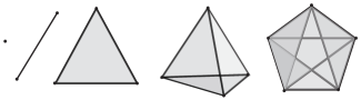
Figure 1: A $p$-simplex is constructed from $\left(p+1\right)$ numbers of $\left(p-1\right)$-simplices: connecting two points construct a segment, connecting three segments construct a triangle, connecting four triangles construct a tetrahedron, connecting five tetrahedra construct a 4-simplex, and so on.

We describe $p$-simplex using $p$-forms. A similar attempt had already been studied in key-3.24 . Any $p$-form $\omega$ can be written as:

$$\omega=\omega_{\left[a_{1}..a_{p}\right]}dx^{a_{1}}\wedge..\wedge dx^{a_{p}},$$ (1)

with $\omega_{\left[a_{1}..a_{p}\right]}$ is an anti-symmetric tensor of order $\tbinom{0}{p}$, given by:

$$\omega_{\left[a_{1}..a_{p}\right]}=\frac{1}{p!}\delta_{a_{1}..a_{p}}^{b_{1}..b_{p}}\omega_{b_{1}..b_{p},}$$

and $\delta_{a_{1}..a_{p}}^{b_{1}..b_{p}}$ is the generalized Kronecker delta, given by:

$$\delta_{a_{1}..a_{p}}^{b_{1}..b_{p}}=\det\left[\begin{array}[]{cccc}\delta_{a_{1}}^{b_{1}}&\delta_{a_{2}}^{b_{1}}&\cdots&\delta_{a_{p}}^{b_{1}}\\ \delta_{a_{1}}^{b_{2}}&\ddots\\ \vdots\\ \delta_{a_{1}}^{b_{p}}&\delta_{a_{2}}^{b_{p}}&\cdots&\delta_{a_{p}}^{b_{p}}\end{array}\right].$$

A 1-form is simply a covariant vector:

$$\mathbf{a}=a_{\mu}dx^{\mu},\qquad\mu=1,..,n.$$

We can costruct $n$-form from several lower forms using the wedge product $\wedge$, for example, a 2-form from two 1-forms:

$$\mathbf{a}\wedge\mathbf{b}=\frac{1}{2}\left(a_{\mu}b_{\nu}-a_{\nu}b_{\mu}\right)dx^{\mu}\wedge dx^{\nu}.$$ (2)

The space of $p$-forms over an $n$-dimensional space $\mathbb{R}^{n}$ is written as $\Omega^{p}\left(\mathbb{R}^{n}\right)$, together with the wedge product $\wedge$, they form an exterior algebra over $\mathbb{R}^{n}$. See key-3.7 ; key-3.8 ; key-3.25 for details. Since the space of $p$-forms $\Omega^{p}\left(\mathbb{R}^{n}\right)$ is a vector space satisfying vector space axioms, we can introduce an inner product operation which give rise to a flat Euclidean metric $g$ to the space $\Omega^{p}\left(\mathbb{R}^{n}\right)$. Using this metric, we could obtain the contraction of two $p$-forms:

$$g\left(\mathbf{a},\mathbf{b}\right) = g\left(a_{\left[\mu...\nu\right]}dx^{\mu}\wedge..\wedge dx^{\nu},b_{\left[\mu^{\prime}...\nu^{\prime}\right]}dx^{\mu^{\prime}}\wedge..\wedge dx^{\nu^{\prime}}.\right)$$

$$= a_{\left[\mu...\nu\right]}b_{\left[\mu^{\prime}...\nu^{\prime}\right]}\varepsilon^{\mu..\nu}\varepsilon^{\mu^{\prime}..\nu^{\prime}},$$

with $\varepsilon^{\mu..\nu}\varepsilon^{\mu^{\prime}..\nu^{\prime}}$ comes from:

$$\varepsilon^{\mu..\nu}\varepsilon^{\mu^{\prime}..\nu^{\prime}}=g\left(dx^{\mu}\wedge..\wedge dx^{\nu},dx^{\mu^{\prime}}\wedge..\wedge dx^{\nu^{\prime}}\right),$$ (4)

which is the tensor product of two Levi-Civita symbol in $n$-dimension. The tensor product of two Levi-Civita symbol is a generalized Kronecker delta, which can be obtained as:

$$\varepsilon^{\mu..\nu}\varepsilon^{\mu^{\prime}..\nu^{\prime}}=\det\left|\begin{array}[]{ccc}\delta^{\mu\mu^{\prime}}&\ldots&\delta^{\mu\nu^{\prime}}\\ \vdots&\ddots&\vdots\\ \delta^{\nu\mu^{\prime}}&\ldots&\delta^{\nu\nu^{\prime}}\end{array}\right|.$$ (5)

In the following subsection, we will give a sketch of the construction of simplices using $p$-forms.

II.1.1 2-simplex (triangle)

A 1-form $\mathbf{l}$ can be interpreted geometrically as a segment with length $\left|\mathbf{l}\right|$, from which we can construct more complex geometries. A 2-simplex or a triangle can only be realized in space with dimension $n\geq 2.$ We can build a 2-simplex $\mathbf{a}$, given two distinct 1-forms: $\left\{\mathbf{l}_{1},\mathbf{l}_{2}\right\}\in T_{p}^{*}\mathcal{M}$ using the wedge product:

$$\mathbf{a}=\frac{1}{2}\left(\mathbf{l}_{1}\wedge\mathbf{l}_{2}\right)\in T_{p}^{*}\mathcal{M}\otimes T_{p}^{*}\mathcal{M},$$

where the components are given by (2). This can be interpreted as the illustration shown in FIG. 2, with $\mathbf{a}$ is the triangle constructed by segment $\mathbf{l}_{1}$ and $\mathbf{l}_{2}$.

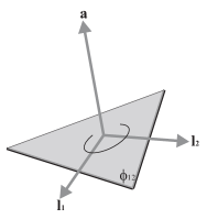
Figure 2: A triangle $\mathbf{a}$ can be obtained by wedge-producting two 1-forms: $\mathbf{l}_{1}$ and $\mathbf{l}_{2}$. $\phi_{12}$ is the angle between these 1-forms.

Using the inner product on $\Omega^{2}\left(\mathbb{R}^{n}\right)$ defined in (II.1), we could obtain the norm of 2-form $\mathbf{a}$,

$$\left|\mathbf{a}\right|=\sqrt{g\left(\mathbf{a},\mathbf{a}\right)},$$

which is interpreted as the area of the triangle.

We consider the boundary of $\mathbf{a}$, constructed from three 1-forms $\partial\mathbf{a}=\left\{\mathbf{l}_{1},\mathbf{l}_{2},\mathbf{l}_{12}\right\},$ with $\mathbf{l}_{12}$ defined as:

$$\mathbf{l}_{12}\doteq\mathbf{l}_{1}+\mathbf{l}_{2},$$ (6)

so that these set of 1-forms satisfy closure condition:

$$\mathbf{l}_{1}+\mathbf{l}_{2}-\mathbf{l}_{12}=0.$$ (7)

Therefore, these set of forms satisfy the triangle inequality:

$$0\leq\left|\left(\mathbf{l}_{1}+\mathbf{l}_{2}\right)\right|\leq\left|\mathbf{l}_{1}\right|+\left|\mathbf{l}_{2}\right|,$$ (8)

since metric $g$ on $\Omega^{2}\left(\mathbb{R}^{n}\right)$ is Riemannian. Their norms can be interpreted as the length of segment of a closed triangle. The boundary $\partial\mathbf{a}$ is an example of a subspace of $\mathbf{a}.$

II.1.2 3-simplex (tetrahedron)

A 3-simplex or a tetrahedron can only be realized in space with dimension $n\geq 3.$ To build a 3-simplex $\mathbf{v}$, we need three distinct 1-forms: $\left\{\mathbf{l}_{1},\mathbf{l}_{2},\mathbf{l}_{3}\right\}\in T_{p}^{*}\mathcal{M}$ so that we could obtain a 3-form:

$$\mathbf{v}=\frac{1}{3}\left(\mathbf{l}_{1}\wedge\mathbf{l}_{2}\wedge\mathbf{l}_{3}\right),$$

see FIG. 3.

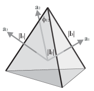
Figure 3: A tetrahedron $\mathbf{v}$ can be obtained by wedge-producting three 1-forms: $\mathbf{l}_{1}$, $\mathbf{l}_{2}$, and $\mathbf{l}_{3}$. $\phi_{ij}$ is the angle between these 1-forms. The wedge product between each two of these 1-forms, say, $\mathbf{l}_{i}$ and $\mathbf{l}_{j}$, construct a triangle $\mathbf{a}_{k}.$

The norm of $\mathbf{v}$ can be obtained by using the metric $g$ as in the triangle case:

$$\left|\mathbf{v}\right|=\sqrt{g\left(\mathbf{v},\mathbf{v}\right)},$$

and this can be interpreted as the volume of a tetrahedron.

Now we consider the subspaces of the tetrahedron. The first subspace is the boundary $\partial\mathbf{v}$ which is the 2-dimensional space of triangles, consisting of four triangles:

$$\partial\mathbf{v}=\left\{\underset{\mathbf{a}_{1}}{\underbrace{\frac{1}{2}\left(\mathbf{l}_{2}\wedge\mathbf{l}_{3}\right)}},\underset{\mathbf{a}_{2}}{\underbrace{\frac{1}{2}\left(\mathbf{l}_{3}\wedge\mathbf{l}_{1}\right)}},\underset{\mathbf{a}_{3}}{\underbrace{\frac{1}{2}\left(\mathbf{l}_{1}\wedge\mathbf{l}_{2}\right)}},\underset{\mathbf{a}_{4}=-\mathbf{a}_{123}}{\underbrace{-\frac{1}{2}\left(\mathbf{l}_{1}\wedge\mathbf{l}_{2}+\mathbf{l}_{2}\wedge\mathbf{l}_{3}+\mathbf{l}_{3}\wedge\mathbf{l}_{1}\right)}}\right\},$$

where the boundary satisfies closure condition:

$$\sum_{i=1}^{4}\mathbf{a}_{i}=0,$$ (9)

which is also known as the Minkowski theorem key-3.5 ; key-3.26 . This is a 2-form analogy to the closure condition in (7). Another subspace of the tetrahedron is the space of segment, which is 1-dimensional:

$$\partial^{2}\mathbf{v}=\left\{\mathbf{l}_{1},\mathbf{l}_{2},\mathbf{l}_{3},\mathbf{l}_{12},\mathbf{l}_{23},\mathbf{l}_{31}\right\},$$

where the norms of every three segments $\left\{\left|\mathbf{l}_{i}\right|,\left|\mathbf{l}_{j}\right|,\left|\mathbf{l}_{ij}\right|\right\}$ and $\left\{\left|\mathbf{l}_{12}\right|,\left|\mathbf{l}_{23}\right|,\left|\mathbf{l}_{31}\right|\right\}$ satisfy triangle inequality (8), but only three triangles satisfy the closure condition as in (7):

$$\mathbf{l}_{i}+\mathbf{l}_{j}-\mathbf{l}_{ij} = 0,\qquad i,j=1,2,3,\quad i\neq j,$$

$$\mathbf{l}_{12}+\mathbf{l}_{23}+\mathbf{l}_{31} \neq 0,\qquad\textrm{(in general).}$$

The reason for this is because the boundary $\partial\mathbf{v}$ is a closed surface homeomorphic to a sphere $\mathcal{S}^{2},$ and to cover a sphere, we need minimal two charts, while in this derivation we only use a single vector space which is $T_{p}^{*}\mathcal{M};$ in other words, we need $\left\{\mathbf{l}_{12},\mathbf{l}_{23},\mathbf{l}_{31}\right\}$ to live in another vector space $T_{q}^{*}\mathcal{M},$ if we want to force them to satisfy triangle inequality.

It can be shown that the wedge product of two 1-forms (and their permutations) meeting at a same point is a triangle:

$$\frac{1}{2}\left(\mathbf{l}_{i}\wedge\mathbf{l}_{j}\right) = \mathbf{a}_{k},\qquad i,j,k=1,2,3,\quad i\neq j\neq k.$$

There is a beautiful hierarchial structure among a simplex with its subspaces.

II.1.3 4-simplex

A 4-simplex is a 4-dimensional analog of a triangle in 2-dimension and a tetrahedron in 3-dimension. Its 2-dimension projection is illustrated in FIG. 4(a). A 4-simplex can only be realized in space with dimension $n\geq 4.$ To build a 4-simplex $\mathbf{s}$, we need four distinct 1-forms, $\left\{\mathbf{l}_{1},\mathbf{l}_{2},\mathbf{l}_{3},\mathbf{l}_{4}\right\}:$

$$\mathbf{s}=\frac{1}{4}\left(\mathbf{l}_{1}\wedge\mathbf{l}_{2}\wedge\mathbf{l}_{3}\wedge\mathbf{l}_{4},\right),$$

see FIG. 4(a).

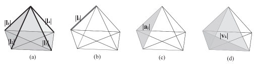
Figure 4: (a) Construction of a 4-simplex by wedge-producting four 1-forms: $\mathbf{l}_{1}$, $\mathbf{l}_{2}$, $\mathbf{l}_{3}$. and $\mathbf{l}_{4}$. (b) the 1-dimensional subspace of a 4-simplex $\mathbf{s}$ consists ten segments $\mathbf{l}_{i}$. (c) the 2-dimensional subspace of $\mathbf{s}$ contains also ten triangle $\mathbf{a}_{j}$. (d) the 3-dimensional subspace of $\mathbf{s}$, which is also its boundary, contains five tetrahedra $\mathbf{v}_{k}$.

The norm of the 4-form $\mathbf{s}$ is:

$$\left|\mathbf{s}\right|=\sqrt{g\left(\mathbf{s},\mathbf{s}\right)},$$

and interpreted as the 4-dimensional ’volume’ of a 4-simplex.

Similar with the previous cases, we could obtain subspaces of the 4-simplex, which now has three types of subspaces. The first subspace is the 1-dimensional subspace, consisting of ten segments:

$$\partial^{3}\mathbf{s}=\left\{\mathbf{l}_{1},\mathbf{l}_{2},\mathbf{l}_{3},\mathbf{l}_{4},\mathbf{l}_{12},\mathbf{l}_{13},\mathbf{l}_{14},\mathbf{l}_{23},\mathbf{l}_{24},\mathbf{l}_{34}\right\},$$

the norms of every three segments $\left\{\left|\mathbf{l}_{i}\right|,\left|\mathbf{l}_{j}\right|,\left|\mathbf{l}_{ij}\right|\right\}$ and $\left\{\left|\mathbf{l}_{ij}\right|,\left|\mathbf{l}_{jk}\right|,\left|\mathbf{l}_{ki}\right|\right\}$ satisfy triangle inequality (8), but only six from ten triangles satisfy the closure condition as in (7):

$$\mathbf{l}_{i}+\mathbf{l}_{j}-\mathbf{l}_{ij} = 0,\qquad i,j=1,2,3,\quad i\neq j,$$

$$\mathbf{l}_{ij}+\mathbf{l}_{jk}+\mathbf{l}_{ki} \neq 0,\qquad\textrm{(in general).}$$

The reason for this is the same with the reason in the lower dimensional case in the previous section.

The second subspace is the 2- dimensional subspace, consisting ten triangles:

$$\partial^{2}\mathbf{s}=\left\{\mathbf{a}_{12},\mathbf{a}_{13},\mathbf{a}_{14},\mathbf{a}_{23},\mathbf{a}_{24},\mathbf{a}_{34},\mathbf{a}_{123},\mathbf{a}_{124},\mathbf{a}_{134},\mathbf{a}_{234}\right\},$$

where:

$$\mathbf{a}_{ij} = \frac{1}{2}\left(\mathbf{l}_{i}\wedge\mathbf{l}_{j}\right),\qquad i,j,k=1,2,3,4\quad i\neq j\neq k.$$

$$\mathbf{a}_{ijk} = -\frac{1}{2}\left(\mathbf{l}_{i}\wedge\mathbf{l}_{j}+\mathbf{l}_{j}\wedge\mathbf{l}_{k}+\mathbf{l}_{k}\wedge\mathbf{l}_{i}\right).$$

Each four of the triangles construct a boundary of a tetrahedron:

$$\partial\mathbf{v}_{l}=\left\{\mathbf{a}_{ij},\mathbf{a}_{jk},\mathbf{a}_{ki},\mathbf{a}_{ijk}\right\},\qquad i,j,k,l=1,2,3,4\quad i\neq j\neq k\neq l,$$

i.e., $\left\{\left|\mathbf{a}_{ij}\right|,\left|\mathbf{a}_{jk}\right|,\left|\mathbf{a}_{ki}\right|,\left|\mathbf{a}_{ijk}\right|\right\}$ and $\left\{\left|\mathbf{a}_{123}\right|,\left|\mathbf{a}_{124}\right|,\left|\mathbf{a}_{134}\right|,\left|\mathbf{a}_{234}\right|\right\}$ satisfy triangle inequality for higher forms, but only $\left\{\mathbf{a}_{ij},\mathbf{a}_{jk},\mathbf{a}_{ki},\mathbf{a}_{ijk}\right\}$ satisfy the closure condition for the same reason as the previous cases.

The last one is the 3- dimensional subspace which is the boundary of the 4-simplex, consisting five tetrahedra:

$$\partial\mathbf{s}=\left\{\mathbf{v}_{1},\mathbf{v}_{2},\mathbf{v}_{3},\mathbf{v}_{4},\mathbf{v}_{5}=-\mathbf{v}_{1234}\right\},$$

with:

$$\mathbf{v}_{l} = \mathbf{l}_{i}\wedge\mathbf{l}_{j}\wedge\mathbf{l}_{k},\qquad i,j,k,l=1,2,3,4\quad i\neq j\neq k\neq l$$

$$\mathbf{v}_{1234} = -\left(\sum_{l=1}^{4}\mathbf{v}_{l}\right).$$

The boundary satisfies 3-form closure condition:

$$\sum_{l=1}^{5}\mathbf{v}_{l}=0.$$

This definition can be easily generalized to $p$-simplex in any dimension.

II.2 Dihedral angles

In Regge geometry, where we have discrete manifold instead of continuous manifold, the intrinsic curvature is defined by angles key-3.19 ; key-3.23 . In this subsection, we will review the definition of angles on a simplices.

II.2.1 The dihedral angles

Having an inner product defined in the space of forms $\Omega^{p}\left(\mathbb{R}^{n}\right)$ using a Euclidean metric $g$, we could have a notion of spherical angle. In general, spherical angle is defined by relation:

$$\cos\phi_{ab}=\frac{g\left(\mathbf{a},\mathbf{b}\right)}{\left|\mathbf{a}\right|\left|\mathbf{b}\right|},$$ (10)

given vectors $\mathbf{a},\mathbf{b},$ and a Riemannian metric $g.$ Since $\Omega^{p}\left(\mathbb{R}^{n}\right)$ is also a vector space, we could use (10) to define angles in the space of forms $\Omega^{p}\left(\mathbb{R}^{n}\right)$.

Let $\mathbf{s}\in\Omega^{4}\left(\mathbb{R}^{4}\right)$ be a 4-form describing a 4-simplex. Inside $\mathbf{s}$, there are segments $\mathbf{l}_{i}$, triangles $\mathbf{a}_{j}$, and tetrahedra $\mathbf{v}_{k}$ as a subspaces of $\mathbf{s.}$ These are 1-forms, 2-forms, and 3-forms respectively. Since in $\Omega^{4}\left(\mathbb{R}^{4}\right)$, $\mathbf{l}_{i}$, $\mathbf{a}_{j}$, and $\mathbf{v}_{k}$ have directions (they have components), they act as vectors, not as scalars. Therefore, we can have three notions of angle inside a 4-simplex $\mathbf{s}$: angles between segments, between triangles, and between tetrahedra. These angles are always located around a hinges, which are the $\left(p-2\right)$-simplices key-3.19 ; key-3.23 .

Dihedral angle on a point.

This angle is defined as the spherical angle between two segments. Given 1-forms $\mathbf{l}_{i}$ and $\mathbf{l}_{j}$ $\in T_{p}^{*}\mathcal{M}$, the 2-dimensional dihedral angle $\phi_{ij}$ on a point is defined as:

$$\phi_{ij}=\pi-\bar{\phi}_{ij},\qquad\cos\bar{\phi}_{ij}=\frac{g\left(\mathbf{l}_{i},\mathbf{l}_{j}\right)}{\left|\mathbf{l}_{i}\right|\left|\mathbf{l}_{j}\right|}.$$ (11)

These angles are located around point $p$ of the 4-simplex, see FIG. 5(a).

Dihedral angle on a segment.

Another angle we have in a 4-simplex is the angle between two triangles (we usually called it as ’dihedral’ angle). This angle is defined by an intersection of two planes, meeting on a segment. Given 2-forms $\mathbf{a}_{i},\mathbf{a}_{j}$, the 3-dimensional dihedral angle $\theta_{ij}$ on a segment is defined as:

$$\theta_{ij}=\pi-\bar{\theta}_{ij},\qquad\cos\bar{\theta}_{ij}=\frac{g\left(\mathbf{a}_{i},\mathbf{a}_{j}\right)}{\left|\mathbf{a}_{i}\right|\left|\mathbf{a}_{j}\right|},$$ (12)

where the inner product of forms is defined in Subsection III A. See FIG. 5(b).

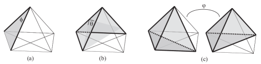
Figure 5: Types of dihedral angle inside a 4-simplex. (a) $\phi$ is the 2-dimensional dihedral angle between two segments, located on a point of the 4-simplex. (b) $\theta$ is the 3-dimensional dihedral angle between two triangles, located on a segment of the 4-simplex. (c) $\varphi$ is the 4-dimensional dihedral angle between two tetrahedra, located on a triangle of the 4-simplex.

Dihedral angle on a plane.

This angle is not common in standard 3-dimensional geometry. It comes from an intersection between two tetrahedra, meeting on a plane. Remember that in 4-dimension or larger, a 3-dimensional geometric figures defined by 3-forms have directions, since the 3-form is not yet a volume form in this space. On 4-dimension, these 3D geometrical figures live in a 4-dimensional vector space spanned by basis $dx^{i}\wedge dx^{j}\wedge dx^{k}.$

Given 3-forms $\mathbf{v}_{i},\mathbf{v}_{j}$, the 4-dimensional dihedral angle $\varphi_{ij}$ on a plane is defined as:

$$\varphi_{ij}=\pi-\bar{\varphi}_{ij},\qquad\cos\bar{\varphi}_{ij}=\frac{g\left(\mathbf{v}_{i},\mathbf{v}_{j}\right)}{\left|\mathbf{v}_{i}\right|\left|\mathbf{v}_{j}\right|},$$

see FIG. 5(c).

In 4-dimension, we can only have forms up to 4-form: $dx^{\mu}\wedge dx^{\nu}\wedge dx^{\sigma}\wedge dx^{\rho}$ , which is a volume-form in $\Omega^{4}\left(\mathbb{R}^{4}\right).$ No higher forms of geometry can be constructed. Therefore, we can only have three types of dihedral angles which are: $\phi$, the angles between segments meeting at a point; $\theta$, the angles between planes meeting at a segments; and $\varphi,$ the angles between 3D spaces meeting on a plane. The next step is to obtain the relation between these dihedral angles through the ’dihedral angle formula’.

II.2.2 Dihedral angle formula

In the standard 3-dimensional Euclidean geometry, we have the remarkable dihedral angle formula of the tetrahedron, which is a relation between $\phi$, the angles between segments of the tetrahedron, and $\theta,$ the angles between planes of the same tetrahedron key-3.27 :

$$\cos\theta{}_{ij,k}=\frac{\cos\phi{}_{ij}-\cos\phi_{ik}\cos\phi_{kj}}{\sin\phi_{ik}\sin\phi_{kj}},$$ (13)

see FIG. 6.

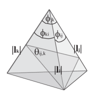
Figure 6: Given angles $\phi_{ij}$, $\phi_{ik}$, $\phi_{jk}$ at point $p$ of a tetrahedron, we could obtain the dihedral angle $\theta{}_{ij,k}$. In fact, $\theta{}_{ij,k}$ is only $\phi_{ij}$ projected on the plane normal to segment $\left|\mathbf{l}_{k}\right|$.

This relation can be derived algebraically using forms, in a relatively simple way. See Appendix A.

Remarkably, as shown in key-3.28 , this dihedral angle relation is valid for any dimension, which means it is a relation between a $p$-dimensional dihedral angle (the angle between $\left(p-1\right)$-simplices) with $\left(p-1\right)$-dimensional dihedral angle (the angle between $\left(p-2\right)$-simplices). The dihedral angle formula can also be written in the inverse form:

$$\cos\phi_{ij}=\frac{\cos\theta_{ij,k}-\cos\theta_{ik,j}\cos\theta_{kj,i}}{\sin\theta_{ik,j}\sin\theta_{kj,i}}.$$ (14)

III Coordinate-free variables

Segments, triangles, and tetrahedra, which are respectively, described by 1-forms, 2-forms, and 3-forms, are basic geometrical elements in 3-dimensional discrete geometry. They are partitions of space: segments are partitions of 1-dimensional space, triangles and more complex polygons are partitions of 2-dimensional space, tetrahedra and polyhedra are partitions of 3-dimensional space, and so on: $n$-polytopes are partitions of $n$-dimensional space. In LQG, quantizing gravitational field will give ’quanta of gravitational field’, but since the gravitational field is the spacetime itself; these ’quanta of gravitational field’, in the canonical framework, can be regarded as ’quanta’ or ’particles’ of space.

It is clear that in discrete geometry, we have a hierarchial structure of spaces: A $p$-simplex is constructed from $\left(p+1\right)$ numbers of $\left(p-1\right)$-simplices. We have already shown in Subsection III A how a $p$-simplex can be constructed from several numbers of lower-dimensional forms, by using the wedge product. This is a vectorial construction, where we explicitly use a specific coordinate system. But since the theory of gravity (and all theory of physics) needs to satisfy the general covariance principle, i.e., the formulation of any physical theory must be valid in all coordinate system, it is convenient to propose a way to write the set of ’coupled-particles’ of spaces, as Regge had proposed, without using coordinates at all: the coordinate-free variables. This will be the main task in this section.

III.1 Single particle of space

III.1.1 The coordinate-free point of view

A $p$-simplex living in an $n$-dimensional space can be described using $p$ numbers of 1-forms, describing a $p$-form. The norm of this $p$-form is interpreted as the $p$-dimensional volume of the $p$-simplex. See FIG. 7.

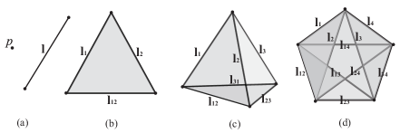
Figure 7: The vectorial picture to describe simplices: (a) A point is a $0$-simplex, it is describe by a scalar and only has trivial information. A flat line or a segment is a $1$-simplex, and it can be completely describe by a 1-form $\mathbf{l}.$ (b) A triangle is a $2$-simplex, it is completely determined by two 1-forms: $\mathbf{l}_{1}$ and $\mathbf{l}_{2}$, the third 1-forms $\mathbf{l}_{12}$ comes form the addition of $\mathbf{l}_{1}$ and $\mathbf{l}_{2}$. (c) A tetrahedron is a 3-simplex, it is completely determined by three 1-forms: $\mathbf{l}_{1},$ $\mathbf{l}_{2}$ and $\mathbf{l}_{3}$, the other three 1-forms, $\mathbf{l}_{ij},$ comes from the addition of $\mathbf{l}_{i}$ and $\mathbf{l}_{j}$. (d) A 4-simplex is completely determined by four 1-forms, while the other six 1-forms are the addition between two of these 1-forms.

It is clear that a $p$-simplex living in $n$-dimensional space needs $pn$ informations to describe these geometries in a vectorial way, completely. These informations, depending on the $n$-dimensional space where the $p$-form is embedded, are more than enough to describe the geometries, because these informations also describe the position and orientation of the geometries with respect to a specific origin $\mathcal{O}$ of the vector space.

This vectorial picture to describe simplices (that is, by using forms) as ’particles’ of spaces, contradicts with one of our basic assumptions used in general relativity: the background independence key-3.34 ; key-3.35 . The first contradiction is the forms live in an $n$-dimensional space $\mathbb{R}^{n},$ which means if we describe the simplices using these forms, then they are embedded in another ’backstage space’ which is $\mathbb{R}^{n}$. We do not want this since we want the simplices to be particles of space. It creates space and it should be the space itself, without referring to any other background stage.

Another contradiction is the notion of ’position’ of the particles of space. This is not satisfactory for the same reason: the particle of space should be the space itself. It should not have a position with respect to another background space, which in turns contradicts the background independence. The ’location’ of the particles of spaces is defined in a ’relational’ way, through the adjacency among particles.

Let us find a way to write these geometrical objects in the coordinate-free picture. See FIG. 8.

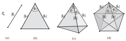
Figure 8: The coordinate-free picture to describe simplices. (a) A point is a $0$-simplex, it is describe by a scalar, which is already coordinate independent. (a) Instead of a 1-form, a flat line or a segment now is described also by a scalar, which is the norm of the 1-form $\left|\mathbf{l}_{1}\right|$. The segment is completely described by this single degrees of freedom, without any information about the origin and the direction. (b) A triangle, in a coordinate-free picture, can be completely determined by three degrees of freedom/ informations: either the norms of the three 1-forms (which are the lengths of the segments of the triangle) $\left\{\left|\mathbf{l}_{1}\right|,\left|\mathbf{l}_{2}\right|,\left|\mathbf{l}_{12}\right|\right\}$, or two norms of 1-forms with the 2D dihedral angle between them: $\left\{\left|\mathbf{l}_{1}\right|,\left|\mathbf{l}_{2}\right|,\phi_{12}\right\}$. Knowing $\left|\mathbf{l}_{12}\right|$, we could obtain $\phi_{12}$ and vice versa. (c) A tetrahedron is completely determined by six degrees of freedom/ informations: either the norms of the six 1-forms $\left\{\left|\mathbf{l}_{1}\right|,\right.$ $\left|\mathbf{l}_{2}\right|,$ $\left|\mathbf{l}_{3}\right|,$ $\left|\mathbf{l}_{12}\right|,$ $\left|\mathbf{l}_{23}\right|,$ $\left.\left|\mathbf{l}_{31}\right|\right\}$, or three norms of 1-forms with three 2D dihedral angles between two of them $\left\{\left|\mathbf{l}_{1}\right|,\right.$ $\left|\mathbf{l}_{2}\right|,$ $\left|\mathbf{l}_{3}\right|,$ $\phi_{12},$ $\phi_{23},$$\left.\phi_{32}\right\}$. (d) At last, a 4-simplex is completely determined by ten degrees of freedom/ informations: either the norms of the ten 1-forms $\left\{\left|\mathbf{l}_{i}\right|,\right.$ $\left|\mathbf{l}_{ij}\right|,$ $i,j=1,2,3,4,$ $\left.i\neq j\right\}$, or four norms of 1-forms with six 2D dihedral angles between two of them $\left\{\left|\mathbf{l}_{i}\right|,\right.$ $\phi_{ij},$ $i,j=1,2,3,4,$ $\left.i\neq j\right\}$.

In this example, we use the lengths of the segments and the 2D dihedral angles as coordinate-free variables. But to prevent ambiguities rising for simplices larger than two, that is, to distinguish if our system contains larger-dimensions simplices (triangles, tetrahedra, etc..) instead of only a set of segments, we use another variables which give equivalent informations of the system.

As an example, for a triangle, we use the following variables: $\left\{\left|\mathbf{a}\right|,\left|\mathbf{l}_{1}\right|,\phi_{12}\right\}$ instead of $\left\{\left|\mathbf{l}_{1}\right|,\left|\mathbf{l}_{2}\right|,\phi_{12}\right\}$, where the area $\left|\mathbf{a}\right|$ will provide us information that our system is a 2-simplex triangle, instead of a system consisting two coupled segments (this will be explained in the next subsection). $\left|\mathbf{a}\right|$ can be obtained by the following transformation:

$$\left|\mathbf{a}\right|=\left|\mathbf{l}_{1}\right|\left|\mathbf{l}_{2}\right|\sin\phi_{12}.$$

For the tetrahedron case, we can use the norm of a 3-form, which is the volume of the tetrahedron, and the norms of the 2-forms, which are areas of triangles, and the 3D dihedral angle between two triangles: $\left\{\left|\mathbf{v}\right|,\left|\mathbf{a}_{1}\right|,\left|\mathbf{a}_{2}\right|,\theta_{12},\theta_{23},\theta_{32}\right\}$ instead of lengths and 2D angles. The transformation is:

$$\left|\mathbf{v}\right|=\frac{1}{3}\left|\mathbf{l}_{j}\right|\left|\mathbf{l}_{k}\right|\left|\mathbf{l}_{l}\right|\sqrt{1+2\cos\phi_{jk}\cos\phi_{kl}\cos\phi_{lj}-\left(\cos^{2}\phi_{jk}+\cos^{2}\phi_{kl}+\cos^{2}\phi_{lj}\right)},$$

$$\left|\mathbf{a}_{i}\right|=\frac{1}{4}\sqrt{\left(\left|\mathbf{l}_{j}\right|+\left|\mathbf{l}_{k}\right|+\left|\mathbf{l}_{jk}\right|\right)\left(-\left|\mathbf{l}_{j}\right|+\left|\mathbf{l}_{k}\right|+\left|\mathbf{l}_{jk}\right|\right)\left(\left|\mathbf{l}_{j}\right|-\left|\mathbf{l}_{k}\right|+\left|\mathbf{l}_{jk}\right|\right)\left(\left|\mathbf{l}_{j}\right|+\left|\mathbf{l}_{k}\right|-\left|\mathbf{l}_{jk}\right|\right)},$$ (15)

$$\cos\theta_{ij,k}=\frac{\cos\phi_{ij}-\cos\phi_{ik}\cos\phi_{kj}}{\sin\phi_{ik}\sin\phi_{kj}},$$ (16)

with (15) is simply the Heron’s formula for a triangle, while (16) is simply the dihedral angle formula. There is a lot of choice of variables to describe a tetrahedron, but we usually choose the sets which gives a unique geometry.

For the 4-simplex case, we could use the norm of the 4-form, $\left|\mathbf{s}\right|,$ which is the volume of the 4-simplex, the volumes of tetrahedra, and the 4D dihedral angle: $\left\{\left|\mathbf{s}\right|,\right.$ $\left|\mathbf{v}_{i}\right|,$ $\left.\varphi_{ij}\right\}$, instead of lengths and 2D angles (it could also be represented by using areas and 3D angle just as in the previous 3D case). See FIG. 9.

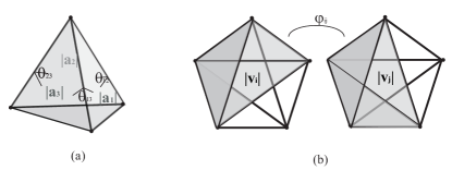
Figure 9: (a) Instead of using lengths (of segments) and 2D angles (between segments) $\left\{\left|\mathbf{l}_{i}\right|,\phi_{ij}\right\}$, we use the volume (of tetrahedron), areas (of the triangle) and 3D angle (between triangles) $\left\{\left|\mathbf{v}\right|,\left|\mathbf{a}_{i}\right|,\theta_{ij}\right\}$ as a coordinate-free variables for a single tetrahedron. (b) Adding 1-dimension higher, we use the volume form of the 4-simplex, 3D volumes (of the tetrahedron) and 4D angle (between tetrahedra) $\left\{\left|\mathbf{s}\right|,\left|\mathbf{v}_{i}\right|,\varphi_{ij}\right\}$ as the coordinate-free variables for a single 4-simplex.

From now on, we will use this coordinate-free picture to describe the degrees of freedom of the geometries.

III.1.2 The choice of variables and uniqueness of a simplex

A simplex is uniquely determined by the lengths of its edges. It must be kept in mind that if we wish to describe the simplices using other variables different than their edges, these sets of variables need to have a one-to-one map to the edges length.

In general, areas and volumes are polynomial (and nonlinear) functions of the length of edges, so the map involving these variables to the set of edges lengths of the simplex may be one-to-many, since polynomial equations in general have more than one solution. This can be simply illustrated in the 2-dimensional case of a triangle specified by its area and two lengths, $\left\{\left|\mathbf{a}\right|,\left|\mathbf{l}_{1}\right|,\left|\mathbf{l}_{2}\right|\right\}$. This choice of variables does not uniquely describe a triangle: there are two different triangles, specified with the three edge lengths $\left\{\left|\mathbf{l}_{1}\right|,\left|\mathbf{l}_{2}\right|,\left|\mathbf{l}_{12}\right|\right\}$ such that both have areas equal to $\mathbf{a}$. This is because the equation expressing the third edge $\mathbf{l}_{12}$ in terms of $\left\{\left|\mathbf{a}\right|,\left|\mathbf{l}_{1}\right|,\left|\mathbf{l}_{2}\right|\right\}$ is a quadratic equation which have two solutions:

$$\left|\mathbf{l}_{12}\right|^{2}=\left|\mathbf{l}_{1}\right|^{2}+\left|\mathbf{l}_{2}\right|^{2}-2\sqrt{\left|\mathbf{l}_{1}\right|^{2}\left|\mathbf{l}_{2}\right|^{2}-4\left|\mathbf{a}\right|^{2}},$$

as long as the length is restricted to be definite positive.

We have classify all possible choices of variables which uniquely describe a Euclidean triangle: $\left\{\left|\mathbf{l}_{i}\right|,\phi_{ij},\phi_{ik}\right\}$ , $\left\{\left|\mathbf{l}_{i}\right|,\phi_{ij},\phi_{jk}\right\}$, $\left\{\left|\mathbf{a}\right|,\phi_{ij},\phi_{ik}\right\}$, $\left\{\left|\mathbf{l}_{i}\right|,\left|\mathbf{l}_{j}\right|,\phi_{ij}\right\}$, and $\left\{\left|\mathbf{a}\right|,\left|\mathbf{l}_{i}\right|,\phi_{ij}\right\}$. Other choice of variables are not well-defined in the sense that the information they contain do not describe uniquely a triangle.

Similar attempts could be done for tetrahedron and 4-simplex case. For a tetrahedron, some unique and well-defined choice of variables are: the volume, two areas of triangles, and three 3D dihedral angles $\left\{\left|\mathbf{v}\right|,\left|\mathbf{a}_{i}\right|,\left|\mathbf{a}_{j}\right|,\theta_{ij},\theta_{ik},\theta_{jk}\right\}$; three areas and three 3D dihedral angles $\left\{\left|\mathbf{a}_{i}\right|,\left|\mathbf{a}_{j}\right|,\left|\mathbf{a}_{k}\right|,\theta_{ij},\theta_{ik},\theta_{jk}\right\}$; and four areas with two 3D dihedral angles $\left\{\left|\mathbf{a}_{i}\right|,\left|\mathbf{a}_{j}\right|,\left|\mathbf{a}_{k}\right|,\left|\mathbf{a}_{ijk}\right|,\theta_{ij},\theta_{jk}\right\}$. The case of a 4-simplex is already studied in key-3.19a , where it turns out that the ten areas of triangles inside a 4-simplex do not completely fix its geometry. We found that some of the unique and well-defined choice of variables for a 4-simplex are: the 4-volume of the 4-simplex, three 3-volumes of tetrahedra, and six 4D dihedral angles $\left\{\left|\mathbf{s}\right|,\left|\mathbf{v}_{i}\right|,\varphi_{jk}\right\}$, $i=1,2,3$, $j,k=1,..,4,$ $j<k$; and four 3-volumes of tetrahedra with six 4D dihedral angles $\left\{\left|\mathbf{v}_{i}\right|,\varphi_{ij}\right\}$, $i,j=1,..,4$, $i<j$. The proofs are given in the Appendix B.

III.2 System of $n$-particles of space

In this subsection, we will return back to the lengths of segments and 2D angles variables, neglecting the ambiguity they brought, for a reason which will be clear later. The use of these variables will not rise any problem to our system, except the ambiguity for the set of $p$-simplices, with $p\geq 1$.

III.2.1 Uncoupled system

Degrees of freedom of a system containing uncoupled $n$-particles of space can be obtained easily, by taking the degrees of freedom of the single particle of space times the number of the particles in the system. For example, using coordinate-free variables, a single segment is completely determined by a single degrees of freedom $\left|\mathbf{l}\right|$, therefore, a system containing two uncoupled segment, say, segment $a$ and $b$, will contains two degrees of freedom $\left\{\left|\mathbf{l}_{a}\right|,\left|\mathbf{l}_{b}\right|\right\}.$ For a higher dimensional case, a system containing three uncoupled triangles $a$, $b$, $c,$ contains $3\times 3=9$ degrees of freedom which are $\left\{\left|\mathbf{l}_{1}^{a}\right|,\left|\mathbf{l}_{2}^{a}\right|,\phi_{12}^{a},\left|\mathbf{l}_{1}^{b}\right|,\left|\mathbf{l}_{2}^{b}\right|,\phi_{12}^{b},\left|\mathbf{l}_{1}^{c}\right|,\left|\mathbf{l}_{2}^{c}\right|,\phi_{12}^{c}\right\};$ and a system containing four uncoupled tetrahedra $a$, $b$, $c,$ $d,$ contains $4\times 6=24$ degrees of freedom, which are $\left\{\left|\mathbf{l}_{1}^{i}\right|,\right.$ $\left|\mathbf{l}_{2}^{i}\right|,$ $\left|\mathbf{l}_{3}^{i}\right|,$ $\phi_{12}^{i},$ $\phi_{23}^{i},$ $\left.\phi_{32}^{i}\right\}$ for $i=a,b,c,d.$ See FIG. 10.

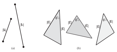
Figure 10: (a) A system of two uncoupled segments $a$ and $b$, containing two degrees of freedom $\left\{\left|\mathbf{l}_{a}\right|,\left|\mathbf{l}_{b}\right|\right\}.$ (b) A system of three uncoupled triangles $a$, $b$, $c,$ containing nine degrees of freedom which are $\left\{\left|\mathbf{l}_{1}^{a}\right|,\left|\mathbf{l}_{2}^{a}\right|,\phi_{12}^{a},\left|\mathbf{l}_{1}^{b}\right|,\left|\mathbf{l}_{2}^{b}\right|,\phi_{12}^{b},\left|\mathbf{l}_{1}^{c}\right|,\left|\mathbf{l}_{2}^{c}\right|,\phi_{12}^{c}\right\}.$

III.2.2 Coupled system

We consider coupled system. To couple two degrees of freedom, we need a ’coupling’, moreover, we define the coupling as a dynamical variable, where each coupling will add another single degrees of freedom to the system. Suppose we have two particles with degrees of freedom $x_{a}$ and $x_{b}$. The natural coupling would be in terms of $g_{ab}$, with $0\leq\left|g_{ab}\right|\leq 1$. $0$ means ’no interaction’ between particle $a$ and $b$, while $1$ means ’maximal interaction’ between them.

In a system of particle of space, we define the coupling $g$ to be the $(p+1)$-dimensional angle between two $p$-simplices, located on the $(p-1)$-simplex. Let us take an example; a system of two coupled segments, say, segment $a$ and $b$, will contain three degrees of freedom $\left\{\left|\mathbf{l}_{a}\right|,\left|\mathbf{l}_{b}\right|,g_{ab}=\cos\phi_{ab}\right\},$ together with the coupling constant. For a higher dimensional case, a system of three coupled triangles $a$, $b$, $c,$ contains twelve degrees of freedom which are $\left\{\left|\mathbf{l}_{1}^{a}\right|,\left|\mathbf{l}_{2}^{a}\right|,\phi_{12}^{a},\left|\mathbf{l}_{1}^{b}\right|,\right.$$\left.\left|\mathbf{l}_{2}^{b}\right|,\phi_{12}^{b},\left|\mathbf{l}_{1}^{c}\right|,\left|\mathbf{l}_{2}^{c}\right|,\phi_{12}^{c}\right\}$, together with the coupling constant $\left\{g_{ab}=\cos\theta_{ab}\right.,$ $g_{ac}=\cos\theta_{ac},$ $\left.g_{bc}=\cos\theta_{bc}\right\}.$ At last, a system containing four coupled tetrahedra $a$, $b$, $c,$ $d,$ contains thirty degrees of freedom which are $\left\{\left|\mathbf{l}_{1}^{i}\right|,\left|\mathbf{l}_{2}^{i}\right|,\left|\mathbf{l}_{3}^{i}\right|,\phi_{12}^{i},\phi_{23}^{i},\phi_{32}^{i}\right\},$ $i=a,b,c,d,$ together with the coupling constant $\left\{g_{ij}=\cos\varphi_{ij}\right\},$ with $i,j=a,b,c,d,$ $i\neq j$. See FIG. 11.

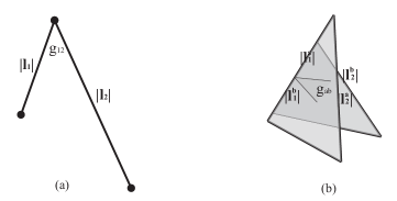
Figure 11: (a) A system containing two coupled segments $a$ and $b$, containing three degrees of freedom $\left\{\left|\mathbf{l}_{a}\right|,\left|\mathbf{l}_{b}\right|,g_{ab}=\cos\phi_{ab}\right\},$ with the coupling constant $g_{ab}$. (b) A system containing two coupled triangles $a$ and $b$, containing seven degrees of freedom which are $\left\{\left|\mathbf{l}_{1}^{a}\right|,\right.$ $\left|\mathbf{l}_{2}^{a}\right|,$ $\phi_{12}^{a},$ $\left|\mathbf{l}_{1}^{b}\right|,$ $\left|\mathbf{l}_{2}^{b}\right|,$ $\phi_{12}^{b},$ $\left.g_{ab}=\cos\theta_{ab}\right\},$ with the coupling constant $g_{ab}$.

III.2.3 Constraint: shape-matching condition

Constraints are specific conditions that must be satisfied by a system or a part of a system. Imposing constraints will reduce the degrees of freedom in a system as many as the number of constraints added key-3.36 ; key-3.37 . In this subsection, we will impose a constraint known as the shape-matching constraint key-3.5 ; key-3.28 , which guarantees the shape of the $\left(p-1\right)$-simplex where the two $p$-simplex meet to be exactly the same. A $\left(p-1\right)$-simplex contains $\frac{p\left(p-1\right)}{2}$ segments (which are $1$-simplices), and two $\left(p-1\right)$-simplices (by neglecting their reflection symmetries) are exactly the same iff all the norm of their $\frac{p\left(p-1\right)}{2}$ segments (which are $1$-simplices) are the same:

$$\left|\mathbf{l}_{i}^{a}\right|\equiv\left|\mathbf{l}_{i}^{b}\right|,\qquad i=1,...,\frac{p\left(p-1\right)}{2}.$$ (17)

Therefore, giving a shape-matching constraint to two coupled $p$-simplices meeting on a common $\left(p-1\right)$-simplex, will reduce their degrees of freedom as many as $\frac{p\left(p-1\right)}{2}$ degrees of freedom. See FIG. 12 as an example.

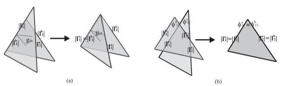
Figure 12: (a) A system of two coupled triangles $a$ and $b$, containing seven degrees of freedom which are $\left\{\left|\mathbf{l}_{1}^{a}\right|,\right.$ $\left|\mathbf{l}_{2}^{a}\right|,$ $\phi_{12}^{a},$ $\left|\mathbf{l}_{1}^{b}\right|,$ $\left|\mathbf{l}_{2}^{b}\right|,$ $\phi_{12}^{b},$ $\left.g_{ab}=\cos\theta_{ab}\right\},$ before imposing constraint on the segment. After imposing the constraint, $\left|\mathbf{l}_{1}^{a}\right|\equiv\left|\mathbf{l}_{1}^{b}\right|,$ the degrees of freedom reduce from seven to six. (b) A system containing two coupled tetrahedra $a$ and $b$, containing thirteen degrees of freedom which are $\left\{\left|\mathbf{l}_{1}^{i}\right|,\right.$ $\left|\mathbf{l}_{2}^{i}\right|,$ $\left|\mathbf{l}_{3}^{i}\right|,$ $\phi_{12}^{i},$ $\phi_{23}^{i},$ $\phi_{32}^{i},$ $\left.g_{ab}=\cos\varphi_{ab}\right\},$ for $i=a,b,$ before imposing constraint on the segments. After imposing three constraints: $\left|\mathbf{l}_{k}^{a}\right|\equiv\left|\mathbf{l}_{k}^{b}\right|,$ $k=1,2,$ and $\phi_{12}^{a}=\phi_{12}^{b}$ on the triangle where the two tetrahedra meet, the degrees of freedom reduce from thirteen to ten.

For a system of simplices containing number of particles $n\geq 3$, the shape matching condition does not satisfy (17), they are much more complicated because we need to be careful not to overcount a same constraint equation twice. The constraint could contain also the dihedral angle relation, restricting the choice of the coupling constant for not being arbitrary, but satisfying (16). Generally, the number of constraints will depend on how each simplex couples to each other. The next task is to obtain the formula for calculating the degrees of freedom.

III.3 Calculating the degrees of freedom

In general, the total degrees of freedom of a system of $n$-particles can be obtained by the following formula:

$$N_{\textrm{d.o.f.}}=nN_{\textrm{degeneracy}}+N_{\textrm{coupling}}-N_{\textrm{constraint}},$$

with $N_{\textrm{degeneracy}}$ is the number of degeneracy inside a single particle, $N_{\textrm{coupling}}$ is the number of the coupling constant, and $N_{\textrm{constraint}}$ is the number of the constraints.

For a system of $n$-particle of space, $N_{\textrm{degeneracy}}$ will depend on the simplices we use; for example, if it is a system of $1$-simplices, a $1$-simplex have no degeneracy, because a segment has only single degrees of freedom. A $2$-simplex have $N_{\textrm{degeneracy}}=3,$ since a triangle have three degrees of freedom. A $3$-simplex have $N_{\textrm{degeneracy}}=6,$ since a tetrahedron have six degrees of freedom. Generalizing, a $p$-simplex have $\frac{p\left(p+1\right)}{2}$ degrees of freedom and therefore:

$$N_{\textrm{degeneracy}}=\frac{p\left(p+1\right)}{2},$$

for a $p$-simplex.

The number of coupling $N_{\textrm{coupling}}$ and the number of the constraints $N_{\textrm{constraint}}$ of a system of $n$-particle of space depend on how each simplex coupled to each other. In other words, it depends on the configuration of the set of simplices to construct the portion of discrete space: it depends on the triangulation, or more general, the tesselation of the simplicial complex key-3.38 ; key-3.39 . Because of this reason, we take a specific, but very useful examples of configuration of simplices called as Pachner-moves, see FIG. 13.

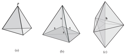
Figure 13: (a) 3-1 Pachner move: three triangles are connected to each others on their edges, constructing an open surface of a tetrahedron, without the bottom triangle closing the surface. The 2D intrinsic curvature is located at point $p$. (b) A 1-dimensional higher analog of (a), the 4-1 Pachner move: four tetrahedra are connected to each others on their internal triangles, constructing an open hypersurface of a 4-simplex, without one tetrahedron closing the hypersurface. The 3D intrinsic curvatures are located on their four hinges: segments $\mathbf{s}$. (c) 3-2 Pachner move: three tetrahedra are connected to each others on their internal triangles, constructing a ’trihedral-bypiramid’. The 3D intrinsic curvature is located on segment $\mathbf{h}$.

We calculate the degrees of freedom of these several Pachner-moves cofigurations. See TABLE 1.

$p$	$N_{\textrm{deg}}$	moves	$n$	$N_{\textrm{d.o.f.}}$	$N_{\textrm{coupling}}$	$N_{\textrm{d.o.f.}}$	$N_{\textrm{const}}$	$N_{\textrm{d.o.f.}}$
				(uncoupled)		(coupled)
1	1	2-1	2	$2\times 1=2$	1	$2+1=3$	0	$3$
2	3	3-1	3	$3\times 3=9$	3	$9+3=12$	$3+3=6$	$12-6=6$
3	6	4-1	4	$4\times 6=24$	6	$24+6=30$	$14+6=20$	$30-20=10$
		3-2	3	$3\times 6=18$	3	$18+3=21$	$8+3=11$	$21-11=10$

Table 1: Degrees of freedom of several Pachner moves configurations.

For the 2-1 move, it is obvious that we have only one coupling $\phi$ and no constraint, so the total degrees of freedom is three, described by $\left\{\left|\mathbf{l}_{1}\right|,\left|\mathbf{l}_{2}\right|,\phi_{12}\right\}.$ For the 3-1 move, we have three triangles where each of them has three degrees of freedom; the number of coupling are three by using the binomial relation $\binom{3}{2}$, the number of constraint are six: three from relation (17) for the segments where these triangles meet, another three from the dihedral angle relation (16) on the coupling constants. Therefore the total degrees of freedom for 3-1 move is six, described by $\left\{\left|\mathbf{a}_{1}\right|,\left|\mathbf{a}_{2}\right|,\left|\mathbf{a}_{3}\right|,\theta_{12},\theta_{13},\theta_{23}\right\},$ to remove ambiguity.

For the 4-1 move, we have four tetrahedron where each of them have six degrees of freedom; the number of coupling are six by using the binomial relation $\binom{4}{2}$, the number of constraint are twenty: fourteen from relation (17) for the segments, six from the dihedral angle relation (16) for the coupling constants. Therefore the total degrees of freedom for 4-1 move is ten, described by $\left\{\left|\mathbf{v}_{i}\right|,\varphi_{ij}\right\}$, $i\neq j=1,2,3,4$ .

The last one, is the 3-2 move: we have three tetrahedron where each of them have six degrees of freedom; the number of coupling are three, the number of constraint are eleven: eight from relation (17) for the segments, three from the dihedral angle relation (16) for the coupling constants. The total degrees of freedom for 3-2 move is also ten, described by its three volumes of tetrahedra, 4D angles between them, three edges length meeting on a common vertex, and a common segment of these tetrahedra: $\left\{\left|\mathbf{v}_{i}\right|,\varphi_{ij},\left|\mathbf{l}_{i}\right|,\left|\mathbf{h}\right|\right\},$ $i\neq j=1,2,3.$ These variables can be proven to describe uniquely the geometry of the polyhedron.

Intrinsic curvatures as an emergent property.

Given the definition of intrinsic curvature of discrete geometry, which is the deficit angle located on the hinge shared by several simplices key-3.19 ; key-3.28 ; key-3.29 , it is clear that curvature can only be defined in a system of coupled $n$-particles of space, in other words, we could think the intrinsic curvature as an emergent property of a many-body system, it is the measure of how strong is the ’interaction’ among the ’particles’ of space.

IV Conclusions

Let us review our relatively new result obtained in this work: We have obtain (1) a way of decribing a set of simplices vectorially by using differential forms, (2) another way of describing a set of simplices using a coordinate-free picture, and (3) a consistent procedure to couple particles of space, together with a way to calculate the degrees of freedom of the system of ’quanta’ of space in the classical framework.

Our last result will be useful when we consider its application to a coarse-graining method of discrete geometry. As a further work, it is interesting if we could obtain a consistent procedure to couple particles of space, and a way to calculate the degrees of freedom of the system of ’quanta’ of space in the twisted geometry framework.

Appendix A (2+1)-dimensional dihedral angle relation

Let $\mathbf{l}_{i},\mathbf{l}_{k}$ be vectors, instead of 1-forms, that is, an element of $T_{p}\mathcal{M}$ instead of $T_{p}^{*}\mathcal{M}$ as in the previous derivation. Therefore we have two relations concerning the dihedral angles:

$$g\left(\mathbf{l}_{i},\mathbf{l}_{k}\right)=\left|\mathbf{l}_{i}\right|\left|\mathbf{l}_{k}\right|\cos\phi_{ik},$$ (18)

$$g\left(\mathbf{l}_{i}\wedge\mathbf{l}_{k},\mathbf{l}_{j}\wedge\mathbf{l}_{k}\right)=\left|\mathbf{l}_{i}\wedge\mathbf{l}_{k}\right|\left|\mathbf{l}_{j}\wedge\mathbf{l}_{k}\right|\cos\theta_{ij,k},$$ (19)

with $\mathbf{l}_{i},$ $\mathbf{l}_{j},$ $\mathbf{l}_{k}$ are vectors.

Step 1:

Using relation (2) concerning the components of a vector 2-forms, we obtain:

$$g\left(\mathbf{l}_{i}\wedge\mathbf{l}_{k},\mathbf{l}_{j}\wedge\mathbf{l}_{k}\right)=2\left(\left(l_{i}\right)_{\mu}\left(l_{k}\right)_{\nu}-\left(l_{i}\right)_{\nu}\left(l_{k}\right)_{\mu}\right)\left(\left(l_{j}\right)_{\rho}\left(l_{k}\right)_{\lambda}-\left(l_{j}\right)_{\lambda}\left(l_{k}\right)_{\rho}\right)\varepsilon^{\mu\nu}\varepsilon^{\rho\lambda},$$ (20)

the basis $dx^{i}\wedge dx^{j}$ can be written as the Levi-Civita symbol $\varepsilon^{ij}.$ In a flat space we can define the metric as:

$$g\left(dx^{\mu}\wedge dx^{\nu},dx^{\rho}\wedge dx^{\lambda}\right)=\varepsilon^{\mu\nu}\varepsilon^{\rho\lambda},$$

following (4). Using the product of two Levi-Civita symbols in (5), we could write the right hand side of (20) as:

$$2\left(\left(l_{i}\right)_{\mu}\left(l_{k}\right)_{\nu}-\left(l_{i}\right)_{\nu}\left(l_{k}\right)_{\mu}\right)\left(\left(l_{j}\right)_{\rho}\left(l_{k}\right)_{\lambda}-\left(l_{j}\right)_{\lambda}\left(l_{k}\right)_{\rho}\right)\left(\delta^{\mu\rho}\delta^{\nu\lambda}-\delta^{\mu\lambda}\delta^{\nu\rho}\right).$$

Doing the tensor algebra, we obtain:

$$g\left(\mathbf{l}_{i}\wedge\mathbf{l}_{k},\mathbf{l}_{j}\wedge\mathbf{l}_{k}\right) = \left(l_{i}\right)_{\mu}\left(l_{j}\right)^{\mu}\left(l_{k}\right)_{\nu}\left(l_{k}\right)^{\nu}-\left(l_{i}\right)_{\mu}\left(l_{k}\right)^{\mu}\left(l_{k}\right)_{\nu}\left(l_{j}\right)^{\nu},$$ (21)

$$= g\left(\mathbf{l}_{i},\mathbf{l}_{j}\right)g\left(\mathbf{l}_{k},\mathbf{l}_{k}\right)-g\left(\mathbf{l}_{i},\mathbf{l}_{k}\right)g\left(\mathbf{l}_{k},\mathbf{l}_{j}\right).$$

Using (18), we could write (21) as:

$$g\left(\mathbf{l}_{i}\wedge\mathbf{l}_{k},\mathbf{l}_{j}\wedge\mathbf{l}_{k}\right)=\left|\mathbf{l}_{i}\right|\left|\mathbf{l}_{k}\right|^{2}\left|\mathbf{l}_{j}\right|\left(\cos\phi_{ij}-\cos\phi_{ik}\cos\phi_{kj}\right).$$ (22)

Step 2:

Now, we try to derive the expression for $\left|\mathbf{l}_{i}\wedge\mathbf{l}_{k}\right|.$ We know that:

$$g\left(\mathbf{l}_{i}\wedge\mathbf{l}_{k},\mathbf{l}_{j}\wedge\mathbf{l}_{k}\right)=\left|\mathbf{l}_{i}\wedge\mathbf{l}_{k}\right|^{2},$$

so using (21):

$$\left|\mathbf{l}_{i}\wedge\mathbf{l}_{k}\right|^{2}=g\left(\mathbf{l}_{i},\mathbf{l}_{i}\right)g\left(\mathbf{l}_{k},\mathbf{l}_{k}\right)-g\left(\mathbf{l}_{i},\mathbf{l}_{k}\right)g\left(\mathbf{l}_{k},\mathbf{l}_{i}\right),$$

then using (18):

$$\left|\mathbf{l}_{i}\wedge\mathbf{l}_{k}\right|^{2}=\left|\mathbf{l}_{i}\right|^{2}\left|\mathbf{l}_{k}\right|^{2}\left(1-\cos^{2}\phi_{ik}\right),$$

or:

$$\left|\mathbf{l}_{i}\wedge\mathbf{l}_{k}\right|=\left|\mathbf{l}_{i}\right|\left|\mathbf{l}_{k}\right|\sin\phi_{ik}.$$ (23)

Step 3:

Inserting (22) and using (23) to (19), we obtain:

$$g\left(\mathbf{l}_{i}\wedge\mathbf{l}_{k},\mathbf{l}_{j}\wedge\mathbf{l}_{k}\right) = \left|\mathbf{l}_{i}\wedge\mathbf{l}_{k}\right|\left|\mathbf{l}_{j}\wedge\mathbf{l}_{k}\right|\cos\theta_{ij,k}$$

$$\left|\mathbf{l}_{i}\right|\left|\mathbf{l}_{k}\right|^{2}\left|\mathbf{l}_{j}\right|\left(\cos\phi_{ij}-\cos\phi_{ik}\cos\phi_{kj}\right) = \left|\mathbf{l}_{i}\right|\left|\mathbf{l}_{k}\right|^{2}\left|\mathbf{l}_{j}\right|\sin\phi_{ik}\sin\phi_{kj}\cos\theta_{ij,k}$$

or:

$$\cos\theta_{ij,k}=\frac{\cos\phi_{ij}-\cos\phi_{ik}\cos\phi_{kj}}{\sin\phi_{ik}\sin\phi_{kj}}.$$ (24)

Appendix B Coordinate-free variables for tetrahedron and 4-simplex

B.1 Tetrahedron

To proof that a set of variables describe uniquely the geometry of a tetrahedron is to show that a set of six unique length of edges can be obtained by a corresponding transformation. Let us start with $\left\{\left|\mathbf{a}_{i}\right|,\left|\mathbf{a}_{j}\right|,\left|\mathbf{a}_{k}\right|,\theta_{ij},\theta_{ik},\theta_{jk}\right\}.$ See FIG. 14.

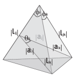
Figure 14: Terminologies of the variables of a tetrahedron.

Using the inverse dihedral angle relation as follows:

$$\cos\phi_{i}=\frac{\cos\theta_{jk}-\cos\theta_{ij}\cos\theta_{ik}}{\sin\theta_{ij}\sin\theta_{ik}},$$ (25)

we could obtain the single-value 2D dihedral angles $\left\{\phi_{i},\phi_{j},\phi_{k}\right\}$ from $\left\{\theta_{ij},\theta_{ik},\theta_{jk}\right\}$ in the range of $0<\phi<\pi$. The next step is to solve the following system of linear equations:

$$\left|\mathbf{a}_{i}\right|=\frac{1}{2}\left|\mathbf{l}_{ij}\right|\underset{\left|\mathbf{h}_{2}\right|}{\underbrace{\left|\mathbf{l}_{ik}\right|\sin\phi_{i},}}$$ (26)

for $\left\{\left|\mathbf{l}_{ij}\right|,\left|\mathbf{l}_{ik}\right|,\left|\mathbf{l}_{jk}\right|\right\}.$ (26) is only the area formula of a triangle. Having three lengths of edges of the tetrahedron (see FIG. 14), we could obtain the remaining three edges from the law of cosine:

$$\left|\mathbf{L}_{i}\right|^{2}=\left|\mathbf{l}_{ij}\right|^{2}+\left|\mathbf{l}_{ik}\right|^{2}-2\left|\mathbf{l}_{ij}\right|\left|\mathbf{l}_{ik}\right|\cos\phi_{i}.$$ (27)

Since we assume the length is positive definite, then we obtain single value of $\left\{\left|\mathbf{L}_{i}\right|,\left|\mathbf{L}_{j}\right|,\left|\mathbf{L}_{k}\right|\right\}.$ Therefore, the map between $\left\{\left|\mathbf{a}_{i}\right|,\left|\mathbf{a}_{j}\right|,\left|\mathbf{a}_{k}\right|,\theta_{ij},\theta_{ik},\theta_{jk}\right\}$ and $\left\{\left|\mathbf{l}_{ij}\right|,\left|\mathbf{l}_{ik}\right|,\left|\mathbf{l}_{jk}\right|,\left|\mathbf{L}_{i}\right|,\left|\mathbf{L}_{j}\right|,\left|\mathbf{L}_{k}\right|\right\}$ is one-to-one.

Let us proof the uniqueness of the next choice of variables: $\left\{\left|\mathbf{a}_{i}\right|,\left|\mathbf{a}_{j}\right|,\left|\mathbf{a}_{k}\right|,\left|\mathbf{a}_{ijk}\right|,\theta_{ij},\theta_{ik}\right\}.$ The easiest way is to obtain the remaining 3D dihedral angle $\theta_{jk}.$ To do this we use the closure condition of the tetrahedron (7) to obtain:

$$\left|\mathbf{a}_{ijk}\right|^{2}=\left|\mathbf{a}_{i}\right|^{2}+\left|\mathbf{a}_{j}\right|^{2}+\left|\mathbf{a}_{k}\right|^{2}-2\left(\left|\mathbf{a}_{i}\right|\left|\mathbf{a}_{j}\right|\cos\theta_{ij}+\left|\mathbf{a}_{i}\right|\left|\mathbf{a}_{k}\right|\cos\theta_{ik}+\left|\mathbf{a}_{j}\right|\left|\mathbf{a}_{k}\right|\cos\theta_{jk}\right).$$ (28)

Solving (28) for $\theta_{jk}$ (which is unique since $0<\theta_{jk}<\pi$) gives the information of $\left\{\left|\mathbf{a}_{i}\right|,\left|\mathbf{a}_{j}\right|,\left|\mathbf{a}_{k}\right|,\theta_{ij},\theta_{ik},\theta_{jk}\right\}$, and the next step to obtain the edges lengths is already obvious from the previous proof. Therefore, the map between $\left\{\left|\mathbf{a}_{i}\right|,\left|\mathbf{a}_{j}\right|,\left|\mathbf{a}_{k}\right|,\left|\mathbf{a}_{ijk}\right|,\theta_{ij},\theta_{ik}\right\}$ and $\left\{\left|\mathbf{l}_{ij}\right|,\left|\mathbf{l}_{ik}\right|,\left|\mathbf{l}_{jk}\right|,\left|\mathbf{L}_{i}\right|,\left|\mathbf{L}_{j}\right|,\left|\mathbf{L}_{k}\right|\right\}$ is one-to-one.

The last proof is for the choice of variables $\left\{\left|\mathbf{v}\right|,\left|\mathbf{a}_{i}\right|,\left|\mathbf{a}_{j}\right|,\theta_{ij},\theta_{ik},\theta_{jk}\right\}.$ For this case, the easiest way is to obtain the single-value 2D dihedral angles $\left\{\phi_{i},\phi_{j},\phi_{k}\right\}$ from $\left\{\theta_{ij},\theta_{ik},\theta_{jk}\right\}$ using (25). The volume of a tetrahedron can be obtained from the relation as follows:

$$\left|\mathbf{v}\right|=\frac{2}{3}\left|\mathbf{a}_{i}\right|\left|\mathbf{a}_{j}\right|\frac{\sin\theta_{ij}}{\left|\mathbf{l}_{ij}\right|},$$ (29)

where we can solve (29) for a unique $\left|\mathbf{l}_{ij}\right|.$ With $\left|\mathbf{l}_{ij}\right|$ known, the other edges length $\left|\mathbf{l}_{ik}\right|$ and $\left|\mathbf{l}_{jk}\right|$ can be obtained from (26). Having the information of $\left\{\phi_{i},\phi_{j},\phi_{k},\left|\mathbf{l}_{ij}\right|,\left|\mathbf{l}_{ik}\right|,\left|\mathbf{l}_{jk}\right|\right\}$ (see FIG. B1), we could obtain the remaining three edges from the law of cosine (27). Therefore, the map between $\left\{\left|\mathbf{v}\right|,\left|\mathbf{a}_{i}\right|,\left|\mathbf{a}_{j}\right|,\theta_{ij},\theta_{ik},\theta_{jk}\right\}$ and $\left\{\left|\mathbf{l}_{ij}\right|,\left|\mathbf{l}_{ik}\right|,\left|\mathbf{l}_{jk}\right|,\left|\mathbf{L}_{i}\right|,\left|\mathbf{L}_{j}\right|,\left|\mathbf{L}_{k}\right|\right\}$ is one-to-one.

B.2 4-simplex

The geometry of a 4-simplex is described uniquely by their ten edges. As a starting point, let us study the variables of a 4-simplex as follows. Let the four edges of 4-simplex be denoted by $\left|\mathbf{l}_{a}\right|$, .., $\left|\mathbf{l}_{d}\right|$, and the six remaining edges be denoted by $\left|\mathbf{l}_{ab}\right|,$ .., $\left|\mathbf{l}_{cd}\right|$. The 2D angle between two edges, say, $\left|\mathbf{l}_{a}\right|$ and $\left|\mathbf{l}_{b}\right|$, is denoted by $\phi_{ab}$. See FIG. 15.

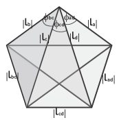
Figure 15: Terminologies of the edges of a tetrahedron.

Now let us denote the four tetrahedra of the 4-simplex by $\left|\mathbf{v}_{i}\right|$, $i=1,..,4$, and the 4D angles between two adjacent tetrahedra $\left|\mathbf{v}_{i}\right|$ and $\left|\mathbf{v}_{j}\right|$ as $\varphi_{ij}$, see FIG. 16.

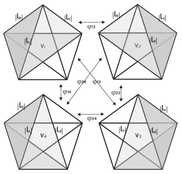
Figure 16: Four tetrahedra (pictured in gray) of the 4-simplex. Each tetrahedron consists six edges; for example, tetrahedron $\left|\mathbf{v}_{1}\right|$ is built from edges $\left|\mathbf{l}_{a}\right|$, $\left|\mathbf{l}_{b}\right|$, $\left|\mathbf{l}_{c}\right|$, $\left|\mathbf{l}_{ab}\right|$, $\left|\mathbf{l}_{ac}\right|$, and $\left|\mathbf{l}_{bc}\right|$. The 4D angle between two tetrahedra is denoted by $\varphi_{ij}$; for example, the 4D angle between tetrahedron $\left|\mathbf{v}_{1}\right|$ and $\left|\mathbf{v}_{2}\right|$ is $\varphi_{12}$.

Let the ’base’ tetrahedron denoted by $\left|\mathbf{v}_{1234}\right|$, as illustrated in FIG. 17.

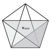
Figure 17: The ’base’ tetrahedron.

The 4D angles $\varphi_{ij}$ are located on a hinge, which is a triangle. See FIG. 18 for an example.

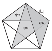
Figure 18: The 4D angles $\varphi_{12}$, $\varphi_{13}$, and $\varphi_{23}$ are located on triangles. These triangles meet on a common edge $\left|\mathbf{l}_{a}\right|.$

The 3D angle $\theta_{i,n}$ is defined as the angle between two triangles which contains $\varphi_{ij}$ and $\varphi_{ik}$, meeting on a common edge $\left|\mathbf{l}_{n}\right|$, see FIG. 19 for examples.

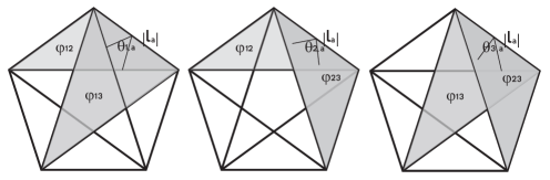
Figure 19: The three triangles where the 4D angles $\left\{\varphi_{12},\varphi_{13},\varphi_{23}\right\}$ are located, defines the 3D angles $\left\{\theta_{1,a},\theta_{2,a},\theta_{3,a}\right\}$ located on $\left|\mathbf{l}_{a}\right|.$

Now, we can start to proof that a set of four 3-volumes of tetrahedra with six 4D dihedral angles $\left\{\left|\mathbf{v}_{i}\right|,\varphi_{ij}\right\}$, $i,j=1,..,4$, $i<j$, describe uniquely the geometry of a 4-simplex. Using the (3+1) dihedral angle relation:

$$\cos\theta_{i,n}=\frac{\cos\varphi_{jk}-\cos\varphi_{ij}\cos\varphi_{ik}}{\sin\varphi_{ij}\sin\varphi_{ik}},$$

we could obtain the 3D angles as follows:

$$\left\{\theta_{1,a},\theta_{2,a},\theta_{3,a}\right\}\, \,\left\{\varphi_{12},\varphi_{13},\varphi_{23}\right\},$$ from

$$\left\{\theta_{1,b},\theta_{2,b},\theta_{4,b}\right\}\, \,\left\{\varphi_{12},\varphi_{14},\varphi_{24}\right\},$$ from

$$\left\{\theta_{1,c},\theta_{3,c},\theta_{4,c}\right\}\, \,\left\{\varphi_{13},\varphi_{14},\varphi_{34}\right\},$$ from

$$\left\{\theta_{2,d},\theta_{3,d},\theta_{4,d}\right\}\, \,\left\{\varphi_{23},\varphi_{24},\varphi_{34}\right\}.$$ from

These 3D angles are in the range of $0<\theta_{i,n}<\pi$ and therefore, unique. Moreover, we classify the 3D dihedral angles according to their tetrahedra: $\theta_{i,n}$ for any $n$ belongs to tetrahedron $\left|\mathbf{v}_{i}\right|,$ see FIG. 20 for example.

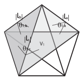
Figure 20: The 3D angles $\theta_{1,a}$, $\theta_{1,b},$ and $\theta_{1,c},$ belongs to tetrahedron $\left|\mathbf{v}_{1}\right|,$ so that they satisfy the (2+1) dihedral angles relation with the 2D angles $\phi$.

Adapting the (2+1) dihedral angle relation (26) with the previous terminologies of the 4-simplex as follows:

$$\cos\phi_{ij}=\frac{\cos\theta_{l,k}-\cos\theta_{l,i}\cos\theta_{l,j}}{\sin\theta_{l,i}\sin\theta_{l,j}},$$

we could obtain six 2D dihedral angles:

$$\left\{\phi_{ab},\phi_{ac},\phi_{bc}\right\}\, \,\left\{\theta_{1,a},\theta_{1,b},\theta_{1,c}\right\},$$ from

$$\left\{\phi_{ab},\phi_{ad},\phi_{bd}\right\}\, \,\left\{\theta_{2,a},\theta_{2,b},\theta_{2,d}\right\},$$ from

$$\left\{\phi_{ac},\phi_{ad},\phi_{cd}\right\}\, \,\left\{\theta_{3,a},\theta_{3,c},\theta_{3,d}\right\},$$ from

$$\left\{\phi_{bc},\phi_{bd},\phi_{cd}\right\}\, \,\left\{\theta_{4,b},\theta_{4,c},\theta_{4,d}\right\}.$$ from

Having the information of six dihedral angles $\left\{\phi_{ab},\phi_{ac},\phi_{ad},\phi_{bc},\phi_{bd},\phi_{cd}\right\}$ and the four volumes of tetrahedra $\left\{\left|\mathbf{v}_{1}\right|,\left|\mathbf{v}_{2}\right|,\left|\mathbf{v}_{3}\right|,\left|\mathbf{v}_{4}\right|\right\}$, we could solve the tetrahedron volume formula:

$$\left|\mathbf{v}_{1}\right| = \frac{1}{3}\left|\mathbf{l}_{a}\right|\left|\mathbf{l}_{b}\right|\left|\mathbf{l}_{c}\right|\sqrt{1+2\cos\phi_{ab}\cos\phi_{ac}\cos\phi_{bc}-\left(\cos^{2}\phi_{ab}+\cos^{2}\phi_{ac}+\cos^{2}\phi_{bc}\right)},$$ (30)

$$\left|\mathbf{v}_{2}\right| = \frac{1}{3}\left|\mathbf{l}_{a}\right|\left|\mathbf{l}_{b}\right|\left|\mathbf{l}_{d}\right|\sqrt{1+2\cos\phi_{ab}\cos\phi_{ad}\cos\phi_{bd}-\left(\cos^{2}\phi_{ab}+\cos^{2}\phi_{ad}+\cos^{2}\phi_{bd}\right)},$$ (31)

$$\left|\mathbf{v}_{3}\right| = \frac{1}{3}\left|\mathbf{l}_{a}\right|\left|\mathbf{l}_{c}\right|\left|\mathbf{l}_{d}\right|\sqrt{1+2\cos\phi_{ac}\cos\phi_{ad}\cos\phi_{cd}-\left(\cos^{2}\phi_{ac}+\cos^{2}\phi_{ad}+\cos^{2}\phi_{cd}\right)},$$ (32)

$$\left|\mathbf{v}_{4}\right| = \frac{1}{3}\left|\mathbf{l}_{b}\right|\left|\mathbf{l}_{c}\right|\left|\mathbf{l}_{d}\right|\sqrt{1+2\cos\phi_{bc}\cos\phi_{bd}\cos\phi_{cd}-\left(\cos^{2}\phi_{bc}+\cos^{2}\phi_{bd}+\cos^{2}\phi_{cd}\right)},$$ (33)

for the four edges $\left\{\left|\mathbf{l}_{a}\right|,\left|\mathbf{l}_{b}\right|,\left|\mathbf{l}_{c}\right|,\left|\mathbf{l}_{d}\right|\right\}$, which is unique for each length.

For the last step, having the information of $\left\{\left|\mathbf{l}_{a}\right|,\left|\mathbf{l}_{b}\right|,\left|\mathbf{l}_{c}\right|,\left|\mathbf{l}_{d}\right|\right\}$ and $\left\{\phi_{ab},..,\phi_{cd}\right\}$, we could obtain six remaining edges of the 4-simplex $\left\{\left|\mathbf{l}_{ab}\right|,..,\left|\mathbf{l}_{cd}\right|\right\}$ from the law of cosine (27). Therefore, the map between $\left\{\left|\mathbf{v}_{i}\right|,\varphi_{ij}\right\}$, $i,j=1,..,4$, $i<j$, and ten edges $\left\{\left|\mathbf{l}_{a}\right|,..,\left|\mathbf{l}_{d}\right|,\left|\mathbf{l}_{ab}\right|,..,\left|\mathbf{l}_{ca}\right|\right\}$ is one-to-one.

Let us proof the uniqueness of the next choice of variables of a 4-simplex: the 4-volume of the 4-simplex, three 3-volumes of tetrahedra, and six 4D dihedral angles $\left\{\left|\mathbf{s}\right|,\left|\mathbf{v}_{i}\right|,\varphi_{jk}\right\}$, $i=1,2,3$, $j,k=1,..,4,$ $j<k$. The ’volume’ (called as area) of a 2D triangle, can be obtained from a conventional area formula (26), which is half of the ’base’ edge times its ’height’ $\left|\mathbf{h}_{2}\right|$. An analog formula is also valid for tetrahedron and 4-simplex key-3.29a . See FIG. 21.

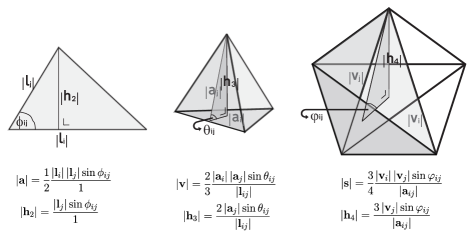
Figure 21: For a triangle, we have a conventional area formula, which is half of the base $\left|\mathbf{l}_{i}\right|$ times its height $\left|\mathbf{h}_{2}\right|.$ For a tetrahedron, a similar formula is valid for the volume, which is one-third of the ’base’, which is now the area of a triangle $\left|\mathbf{a}_{i}\right|$, times its height $\left|\mathbf{h}_{3}\right|.$ Moreover, we could obtain an analog for a 4-simplex: a quarter of the ’base’, which, recursively, is the volume of a tetrahedron, times its height $\left|\mathbf{h}_{4}\right|.$

The volume of a 4-simplex could be written as:

$$\left|\mathbf{s}\right|=\frac{3}{4}\frac{\left|\mathbf{v}_{i}\right|\left|\mathbf{v}_{j}\right|\sin\varphi_{ij}}{\left|\mathbf{a}_{ij}\right|},$$ (34)

given two volumes of tetrahedra $\left|\mathbf{v}_{i}\right|$ and $\left|\mathbf{v}_{j}\right|$ meeting on a common triangle $\left|\mathbf{a}_{ij}\right|.$ This is a 4-dimensional analog to (26) and (29). Let us choose $i=1$ and $j=2,$ so that

$$\left|\mathbf{s}\right|=\frac{3}{4}\frac{\left|\mathbf{v}_{1}\right|\left|\mathbf{v}_{2}\right|\sin\varphi_{12}}{\left|\mathbf{a}_{12}\right|},$$

see FIG. 16. It is clear that we can write $\left|\mathbf{a}_{12}\right|$ as:

$$\left|\mathbf{a}_{12}\right|=\frac{1}{2}\left|\mathbf{l}_{a}\right|\left|\mathbf{l}_{b}\right|\sin\phi_{ab},$$

so that we have:

$$\left|\mathbf{s}\right|=\frac{3}{2}\frac{\left|\mathbf{v}_{1}\right|\left|\mathbf{v}_{2}\right|}{\left|\mathbf{l}_{a}\right|\left|\mathbf{l}_{b}\right|}\frac{\sin\varphi_{12}}{\sin\phi_{ab}}.$$ (35)

Our choice of variables of the 4-simplex are $\left\{\left|\mathbf{s}\right|,\left|\mathbf{v}_{i}\right|,\varphi_{jk}\right\}$, $i=1,2,3$, $j,k=1,..,4,$ $j<k$. From the six 4D angles $\varphi_{jk}$, $j,k=1,..,4,$ we could obtain six unique 2D angles $\left\{\phi_{ab},..,\phi_{cd}\right\}$ by the previous derivation. But this time, we only have the information of three volumes of tetrahedra, instead of four, so we only have equation (30), (31) and (32). To solve these equations for four edges $\left\{\left|\mathbf{l}_{a}\right|,\left|\mathbf{l}_{b}\right|,\left|\mathbf{l}_{c}\right|,\left|\mathbf{l}_{d}\right|\right\}$, we need one more equation, which comes from the 4-simplex volume relation (35). Having unique value of $\left\{\left|\mathbf{l}_{a}\right|,\left|\mathbf{l}_{b}\right|,\left|\mathbf{l}_{c}\right|,\left|\mathbf{l}_{d}\right|\right\}$, with their 2D angles, we could obtain six remaining edges of the 4-simplex $\left\{\left|\mathbf{l}_{ab}\right|,..,\left|\mathbf{l}_{cd}\right|\right\}$ from the law of cosine (27) just as the previous derivation. Therefore, the map between $\left\{\left|\mathbf{s}\right|,\left|\mathbf{v}_{i}\right|,\varphi_{jk}\right\}$, $i=1,2,3$, $j,k=1,..,4,$ $j<k$, and ten edges $\left\{\left|\mathbf{l}_{a}\right|,..,\left|\mathbf{l}_{d}\right|,\left|\mathbf{l}_{ab}\right|,..,\left|\mathbf{l}_{ca}\right|\right\}$ is one-to-one.

References

- (1) T. Regge. General relativity without coordinates. Nuovo Cim. 19 (1961) 558. http://www.signalscience.net/files/Regge.pdf
- (2) L. Lehner. Numerical Relativity: A review. Class. Quant. Grav. 18: R25-R86. (2001). arXiv:gr-qc/0106072
- (3) C. Rovelli. Loop Quantum Gravity. Living Rev. Relativity 1. (1998). http://www.livingreviews.org/lrr-1998-1.
- (4) C. Rovelli. Quantum Gravity. Cambridge Monographs on Mathematical Physics. (2004).
- (5) C. Rovelli, P. Upadhya. Loop quantum gravity and quanta of space: a primer. arXiv:gr-qc/9806079.
- (6) L. Smolin. Atoms of Space and Time. Scientific American 23, pp. 94-103. (2014).
- (7) E. Bianchi, P. Dona’, S. Speziale. Polyhedra in loop quantum gravity. Phys. Rev. D 83: 044035. (2011). arXiv:gr-qc/1009.3402.
- (8) H. Sahlmann, T. Thiemann, O. Winkler. Coherent states for canonical quantum general relativity and the infinite tensor product extension. Nucl. Phys. B 606: 401–440. (2001). arXiv:gr-qc/0102038.
- (9) B. Dittrich. The continuum limit of loop quantum gravity -a framework for solving the theory. (2014). arXiv:gr-qc/1409.1450.
- (10) M. Bojowald. The semiclassical limit of loop quantum cosmology. Class. Quant. Grav. 18: L109-L116. (2001). arXiv:gr-qc/0105113.
- (11) T. Regge, R. M. Williams. Discrete structures in gravity. J. Math. Phys. 41, 3964 (2000). arXiv:gr-qc/0012035v1.
- (12) C. Rovelli, F. Vidotto. Covariant Loop Quantum Gravity: An Elementary Introduction to Quantum Gravity and Spinfoam Theory. UK. Cambridge University Press. ISBN 978-1-107-06962-6. 2015.
- (13) J. W. Barrett and I. Naish-Guzman. The Ponzano-Regge model. Class. Quant. Grav. 26: 155014 (2009). arXiv:gr-qc/0803.3319.
- (14) J. Roberts. Classical 6j-symbols and the tetrahedron. Geom. Topol. 3. (1999). arXiv:math-ph/9812013.
- (15) B. Dittrich. From the discrete to the continuous - towards a cylindrically consistent dynamics. New Journal of Physics 14. (2012). arXiv:gr-qc/1205.6127.
- (16) B. Dittrich, S. Steinhaus. Time evolution as refining, coarse graining and entangling. New Journal of Physics 16. (2014). arXiv:gr-qc/1311.7565.
- (17) E. R. Livine, D. R. Terno. Reconstructing Quantum Geometry from Quantum Information: Area Renormalisation: Coarse-Graining and Entanglement on Spin Networks. arXiv:gr-qc/0603008
- (18) M. Barenz. General Covariance and Background Independence in Quantum Gravity. arXiv:gr-qc/1207.0340.
- (19) L. Freidel, S. Speziale Twisted geometries: A geometric parametrisation of SU(2) phase space. Phys. Rev. D 82: 084040. (2010). arXiv:gr-qc/1001.2748.
- (20) L. Freidel, E. R. Livine. The Fine Structure of SU(2) Intertwiners from U(N) Representations. J. Math. Phys. 51: 082502. (2010). arXiv:gr-qc/0911.3553.
- (21) L. Freidel, S. Speziale. From twistors to twisted geometries. Phys. Rev. D 82: 084041. (2010). arXiv:gr-qc/1006.0199.
- (22) S. Ariwahjoedi, J. S. Kosasih, C. Rovelli, F. P. Zen. How many quanta are there in a quantum spacetime?. Class. Quant. Grav. 32: 16 (2015). arXiv:gr-qc/1404.1750.
- (23) H. S. M. Coxeter. Regular Polytopes. New York: Dover Publications. ISBN 978-0-486-61480-9. (1973).
- (24) B. Grnbaum, V. Kaibel, V. Klee, G. M. Ziegler, eds., Convex polytopes (2nd ed.), New York & London: Springer-Verlag. ISBN 0-387-00424-6. (2003).
- (25) G. M. Ziegler. Lectures on Polytopes. Graduate Texts in Mathematics 152. Berlin, New York: Springer-Verlag. (1995).
- (26) J. W. Barrett, L. Crane. Relativistic spin networks and quantum gravity. J. Math. Phys. 39 (39): 3296–3302. (1998). arXiv:gr-qc/9709028.
- (27) J. W. Barrett, L. Crane. A Lorentzian signature model for quantum general relativity. Class. Quant. Grav. 17: 3101-3118. (2000). arXiv:gr-qc/9904025
- (28) J. Frauendiener. Discrete differential forms in general relativity. Class. Quant. Grav. 23: S369–S385. (2006).
- (29) M. Nakahara. Geometry, Topology and Physics. Second Edition. Taylor & Francis Group. ISBN-13: 978-0750306065. (2003).
- (30) T. Frankel. Geometry of Physics. Cambridge University Press. ISBN-13: 978-1107602601. (2011)
- (31) J. C. Baez, J. P. Muniain. Gauge Fields, Knots, and Gravity. Series on Knots and Everything: vol 4. World Scientific Pub Co Ltd. ISBN 9789810220341. (1994).
- (32) R. Schneider. Convex bodies: the Brunn-Minkowski theory. Encyclopedia of Mathematics and its Applications. ISBN: 9781107601017. (2013).
- (33) E. W. Weisstein. Law of Cosines. MathWorld - A Wolfram Web Resources. http://mathworld.wolfram.com/LawofCosines.html.
- (34) B. Dittrich, S. Speziale. Area-angle variables for general relativity. New. J. Phys. 10: 083006. (2008). arXiv:gr-qc/0802.0864.
- (35) A. Ashtekar, J. Lewandowski. Background Independent Quantum Gravity: A Status Report. Class.Quant.Grav. 21: R53. (2004). arXiv:gr-qc/0404018.
- (36) J. W. Barrett, M. Rocek, R. M. Williams. A note on area variables in Regge calculus. Class.Quant.Grav. 16: R53. (1999). arXiv:gr-qc/9710056.
- (37) H. Goldstein, C. P. Poole (Jr), J. L. Safko. Classical Mechanics. (3rd edition). Addison-Wesley. (2001).
- (38) P. A. M. Dirac. Lectures on Quantum Mechanics. Snowball Publishing. ISBN-13: 978-1607964322. (2012).
- (39) T. Thiemann. Introduction to Modern Canonical Quantum General Relativity. (2001). arXiv:gr-qc/0110034.
- (40) D. Oriti. Approaches to Quantum Gravity: Toward a New Understanding of Space, Time and Matter. Cambridge University Press. ISBN-13: 978-0521860451. (2009).
- (41) S. Ariwahjoedi, J. S. Kosasih, C. Rovelli, F. P. Zen. Curvatures and discrete Gauss-Codazzi equation in (2+1)-dimensional loop quantum gravity. IJGMMP 12: 1550112. (2015). arXiv:gr-qc/1503.05943.
- (42) K. Brown. Simplex Volumes and the Cayley-Menger Determinant. http://www.mathpages.com.