Simulation of Binary Black Hole Spacetimes with a Harmonic Evolution Scheme

Abstract

A numerical solution scheme for the Einstein field equations based on generalized harmonic coordinates is described, focusing on details not provided before in the literature and that are of particular relevance to the binary black hole problem. This includes demonstrations of the effectiveness of constraint damping, and how the time slicing can be controlled through the use of a source function evolution equation. In addition, some results from an ongoing study of binary black hole coalescence, where the black holes are formed via scalar field collapse, are shown. Scalar fields offer a convenient route to exploring certain aspects of black hole interactions, and one interesting, though tentative suggestion from this early study is that behavior reminiscent of “zoom-whirl” orbits in particle trajectories is also present in the merger of equal mass, non-spinning binaries, with appropriately fine-tuned initial conditions.

I Introduction

The past year has seen a remarkable leap in progress toward a numerical solution of the binary black hole problem. The first stable evolution of an entire merger process—orbit, merger, ringdown and gravitational wave extraction—was presented in paper2 using a harmonic formulation of the field equations. Shortly afterwards two groups utb ; nasa independently achieved similar success using a modified form of the BSSN (or NOK) nok ; bs ; sn formulation of the field equations. These first results all focused on the merger of equal mass, non-rotating black holes, and follow-up studies utb2 ; nasa2 are now honing in on a consistent picture of the gravitational waves emitted by such an event. Recently, similar techniques to those employed in utb ; nasa were successfully used to study unequal mass mergers penn ; nasa3 and provide estimates of the “kick” velocity imparted to the final black hole, and in utb3 the effects of black hole spin, aligned and anti-aligned with the orbital angular momentum, were studied, demonstrating that in the aligned case some orbital “hang-up” occurs to radiate away the excess angular momentum.

One reason why the new results seem like such a leap is that progress during earlier years had been rather slow and arduous. For example, it had taken roughly 7 years from the first simulation of a fraction of a non head-on collision bruegmann to a full orbitbruegmann_et_al , with many groups making advances along the way. Much of the effort was also (and still is) focused on understanding the underlying structure of the field equations of general relativity, and why they are so problematic to discretize successfully in many cases. Nevertheless, the manner in which advances had been made over the pass decade suggested a similar series of “baby steps” toward a future solution, which is why the results of the past year have been so exciting.

The primary purpose of this paper is to describe in detail certain aspects of the generalized harmonic (GH) evolution scheme that are of relevance to the simulation of binary black hole (BBH) spacetimes, as first presented in paper1 ; paper2 . This is not a comprehensive overview of the code or technique, and could be viewed as a supplement to paper1 ; paper2 (and see also new_lindblom_et_al for an excellent description of GH evolution). A secondary goal is to relate progress on an ongoing effort to understand the nature of BBH spacetimes produced by scalar-field collapse. It is arguable how relevant such spacetimes may eventually be to gravitational wave detection efforts, nevertheless they offer an easy route to explore a wide range of BBH parameter space. One interesting though tentative result from this early study is that the zoom-whirl type behavior seen in geodesics around black holes may also be present in BBH orbits involving comparable mass components. In particular, what is shown is that for equal mass binaries on non-circular orbits, and with appropriate fine-tuning of the initial conditions, the black holes approach one another, “whirl” around for several orbits, then separate again.

The outline of the rest of the paper is as follows. In Sec. II a brief overview of the Einstein field equations in harmonic form with dynamically evolved source functions and constraint damping terms is given. Sec. III contains a description of parts of the numerical code that seem to be important for stable evolution of BBH spacetimes with this scheme, including excision and numerical dissipation. The effects of constraint damping and the choice of source function evolution equations on a select set of simulations is presented in Sec. IV. Results from the inspiral and merger of scalar field generated BBH spacetimes are given in Sec. V, followed by concluding remarks in Sec. VI.

II Generalized Harmonic Coordinates

In this section a brief description of generalized harmonic coordinates, in the specific form that is discretized in the code, is given. For a thorough description and the history of the use of these coordinates see new_lindblom_et_al .

Consider a spacetime describe by the line element $ds$, metric tensor $g_{ab}$ and coordinates $x^{a}$

$$ds^{2}=g_{ab}dx^{a}dx^{b},$$ (1)

and the Einstein field equations in the form

$$R_{ab}=8\pi\left(T_{ab}-\frac{1}{2}g_{ab}T\right),$$ (2)

where $R_{ab}$ is the Ricci tensor, $g_{ab}$ is the metric tensor, $T_{ab}$ is the stress energy tensor with trace $T$, and units have been chosen so that Newton’s constant $G$ and the speed of light $c$ are equal to 1. The Ricci tensor is defined in terms of the Christoffel symbols $\Gamma^{c}_{ab}$

$$\Gamma^{c}_{ab}=\frac{1}{2}g^{ce}\left[g_{ae,b}+g_{be,a}-g_{ab,e}\right]$$ (3)

via

$$R_{ab}=\Gamma^{d}_{ab,d}-\Gamma^{d}_{db,a}+\Gamma^{e}_{ab}\Gamma^{d}_{ed}-\Gamma^{e}_{db}\Gamma^{d}_{ea}$$ (4)

The notation $f_{,a}$ and $\partial_{a}f$ is used interchangeably to denote ordinary differentiation of some quantity $f$ with respect to the coordinate $x^{a}$.

Harmonic coordinates are defined by the following set of four conditions on the four spacetime coordinates:

$$\Box x^{c}=0,$$ (5)

where $\Box$ is the usual covariant scalar wave operator:

$$\Box x^{c}=\nabla_{b}\nabla^{b}x^{c}=\frac{1}{\sqrt{-g}}\partial_{a}\left(\sqrt{-g}g^{ac}\right).$$ (6)

Generalized harmonic (GH) coordinates introduce a set of arbitrary source functions $H^{c}$ into the definition (5):

$$\Box x^{c}=H^{c}.$$ (7)

Note that in contrast to harmonic coordinates (5), GH coordinates (7) are not conditions on the spacetime coordinates—any geometry in any coordinate system can be expressed in GH form with (7) defining the corresponding source functions.

Using the definitions above, and defining $H_{c}=g_{ac}H^{a}$, the Einstein equations (2) can be rewritten in the following equivalent form, which shall be referred to as the generalized harmonic decomposition of the field equations:

$$\frac{1}{2}g^{cd}g_{ab,cd}+g^{cd}{}_{(,a}g_{b)d,c}+H_{(a,b)}-H_{d}\Gamma^{d}_{ab}$$

$$+\Gamma^{c}_{bd}\Gamma^{d}_{ac}=-8\pi\left(T_{\alpha\beta}-\frac{1}{2}g_{\alpha\beta}T\right)$$ (8)

The utility of the GH decomposition in a numerical evolution (as first carried out in garfinkle ; szilagyi_et_al ; szilagyi_winicour , and also babiuc_et_al1 ; new_lindblom_et_al ; babiuc_et_al ) comes from considering the $H_{c}$ as independent functions; (8) then becomes a set of ten manifestly hyperbolic equations for the ten metric elements $g_{ab}$. As $H_{c}$ are now four independent functions, one needs to provide four additional, independent differential equations to solve for them, schematically written as

$${\mathcal{L}}_{c}H_{c}=0\ \ \ \mbox{(no summation)}.$$ (9)

${\mathcal{L}}_{c}$ is a differential operator that in general depends on the spacetime coordinates, metric and source functions. To complete the specification of the system one needs to provide evolution equations for matter sources, which couple to the field equations through the stress energy tensor. The only matter field considered here is a massless scalar field $\Phi$ that satisfies the wave equation

$$\Box\Phi=0,$$ (10)

and has a stress energy tensor

$$T_{ab}=2\Phi_{,a}\Phi_{,b}-g_{ab}\Phi_{,c}\Phi^{,c},$$ (11)

A solution to (8), (9) and (10) will be a solution to the Einstein equations as long as the GH condition (7) is satisfied for all time. In theory, this is straight-forward to achieve. Define the GH constraint functions $C^{a}$ by

$$C^{a}\equiv H^{a}-\Box x^{a}.$$ (12)

Any solution to the Einstein equations must have $C^{a}=0$. Using the contracted Bianchi identity and conservation of stress energy, one can show that $C^{a}$ satisfies the following homogeneous wave equation

$$\Box C^{a}=-R^{a}{}_{b}C^{b}.$$ (13)

Therefore, what needs to be done to ensure that (8), (9) and (10) satisfy the Einstein equations for all time $t$ is to choose initial conditions for $g_{ab}$ and $H_{a}$ such that $C^{a}=0$ and $\partial_{t}C^{a}=0$ at $t=0$, boundary conditions on $g_{ab}$ and $H_{a}$ such that $C^{a}=0$ on the boundary for all time, and couple this to matter that conserves stress energy. Then (13) guarantees that $C^{a}=0$ throughout the interior 4-volume of the spacetime.

Of course, things are not as simple as this in practice. In a numerical simulation one can only satisfy the conditions described in the preceding paragraph to within the truncation error of the numerical scheme. Again, in principle this is not a problem, however it turns out that in many situations the truncation errors grow too rapidly to achieve useful results given limited resolution. There is good evidence that one of the reasons for the rapid growth of truncation error is not a poor choice of a numerical algorithm, rather (13) admits rapidly growing solutions (so called “constraint violating modes”) given initial data where $C^{a}$ is of order the truncation error. An effective way of dealing with this problem is the addition of constraint damping terms to the equations.

II.1 Constraint Damping

As introduced by Gundlach et al.gundlach_et_al , building on the idea of so-called $\lambda$ systems lambda_ref , the field equations with constraint damping are

$$\frac{1}{2}g^{cd}g_{ab,cd}+g^{cd}{}_{(,a}g_{b)d,c}+H_{(a,b)}-H_{d}\Gamma^{d}_{ab}$$

$$+\Gamma^{c}_{bd}\Gamma^{d}_{ac}+\kappa\left(n_{(a}C_{b)}-\frac{1}{2}g_{ab}n^{d}C_{d}\right)$$

$$=-8\pi\left(T_{\alpha\beta}-\frac{1}{2}g_{\alpha\beta}T\right),$$ (14)

where $\kappa$ is a parameter multiplying the new terms, $n_{a}$ a timelike vector, and $C_{a}$ are the constraints (13). Since the new terms are proportional to the constraints, a solution to the Einstein equations (2) will also be a solution to (14); furthermore, for general solutions of (14) the constraints still satisfy a homogeneous wave equation

$$\Box C^{a}=-R^{a}{}_{b}C^{b}+2\kappa\nabla_{b}\left[n^{(b}C^{a)}\right],$$ (15)

and thus the prescription outlined in the previous section for obtaining valid solutions to the Einstein equations can also be applied using (14) instead of (8). Gundlach et al. have shown that for perturbations about Minkowski spacetime, all finite wavelength solutions to (15) are exponentially damped in time. It is not known whether similar modifications to other forms of the field equations can be made that will also have this desirable constraint damping property, though in gundlach_et_al it was shown how to apply constraint damping to the $Z4$ formalism z4 , and recently Lindblom et al.new_lindblom_et_al described a first order symmetric hyperbolic version of the GH decomposition with constraint damping. In a first order form of the equations additional constraints are introduced that could also exhibit poor behavior with regards to being satisfied in a numerical evolution, though new_lindblom_et_al describe an effective method for dealing with this problem.

In gundlach_et_al it was suggested that $n^{a}$ in (14) could be any timelike vector field; here, for simplicity, $n^{a}$ is chosen to be the unit timelike vector normal to $t\equiv x^{0}={\rm const.}$ surfaces. Specifically, $n_{a}=-\alpha\partial_{a}t$, with $\alpha=\sqrt{-1/g^{tt}}$ being the usual lapse function.

II.2 Source Function Evolution

Within the GH decomposition one can think of the source functions $H_{a}$ as representing the four coordinate degrees of freedom available in general relativity. There are many conceivable ways of choosing $H_{a}$—see paper1 for a more general discussion of some possibilities, and friedrich2 ; balakrishna_et_al ; alcubierre_et_al ; lindblom_scheel ; alcubierre_et_al_2 ; bona_et_al ; bona_et_al_2 for coordinate conditions that might be readily applicable to GH evolution. The focus here will be on one class of equations that have proven useful for binary black hole evolutions, namely:

$$\Box H_{t}=-\xi_{1}\frac{\alpha-1}{\alpha^{\eta}}+\xi_{2}H_{t,\nu}n^{\nu},\ \ \ H_{i}=0.$$ (16)

This equation for $H_{t}$ is a damped wave equation with forcing function designed to prevent the lapse from deviating too far from its Minkowski value of $1$. The parameter $\xi_{2}$ controls the damping term, and $\xi_{2},\eta$ regulate the forcing term. The GH numerical code descrided here tends to develop instabilities in pure harmonic gauge when the lapse function becomes on the order of $0.1$ near the horizon of black holes; equation (16) prevents this from happening. It is unclear whether the instabilities are numerical in nature or an indication that the harmonic gauge is developing a coordinate pathology. However, this is not a crucial question to answer at the moment given the limited availability of computational resources to fully explore the issue, and that (16) works well. In Sec. IV examples of the effect of (16) with a few different parameters are shown.

II.3 Boosted Scalar Field Initial Data

An easy way to produce binary black hole “initial” data is to use scalar field gravitational collapse. At $t=0$ one begins with two Lorentz boosted scalar field profiles with initial amplitude, separation and boost parameters to approximate the kind of orbit that the black holes, which form as the scalar field collapses, will have. On roughly the light crossing time scale of the orbit the remnant scalar field that did not fall into either black hole propagates away from the vicinity of the orbit, leaving behind a good approximation to a vacuum BBH system.

The procedure used to calculate the initial geometry is based on standard techniques cook . One starts with a metric written in ADM ADM form

$$ds^{2}=-\alpha^{2}dt^{2}+h_{ij}\left(dx^{i}+\beta^{i}dt\right)\left(dx^{j}+\beta^{j}dt\right),$$ (17)

where as before $\alpha$ is the lapse, $\beta^{i}$ the shift vector and $h_{ij}$ is the metric intrinsic to $t={\rm const.}$ surfaces. The extrinsic curvature of $h_{ij}$ is defined as

$$K_{ij}=-h_{i}{}^{l}h_{j}{}^{m}\nabla_{m}n_{l}.$$ (18)

In the ADM decomposition the Hamiltonian and momentum constraint equations take on the following form:

$${}^{(3)}R+K^{2}-K_{ab}K^{ab}=16\pi\rho,$$ (19)

$$\nabla_{b}K_{a}{}^{b}-\nabla_{a}K=8\pi J_{a},$$ (20)

where ${}^{(3)}R$ is the trace of the Ricci tensor of the spatial metric, $K$ is the trace of the extrinsic curvature, $\rho$ is the energy density and $J_{a}$ the momentum density of the matter in the spacetime:

$$\rho = T_{ab}n^{a}n^{b},$$ (21)

$$J_{a} = -T_{lm}h^{l}{}_{a}n^{m}.$$ (22)

For the results described here the following initial conditions for the geometry are chosen at $t=0$: the spatial metric and its first time derivative is conformally flat:

$$h_{ij}|_{t=0}=\psi\cdot\eta_{ij}$$ (23)

$$\partial_{t}h_{ij}|_{t=0}=\partial_{t}\psi\cdot\eta_{ij}$$ (24)

where $\psi$ is the conformal factor, and $\eta_{ij}$ is the flat Euclidean metric; the initial slice is maximal:

$$K=0,\ \ \ \partial_{t}K=0$$ (25)

and the initial slice is harmonic:

$$H_{t}=0,\ \ \ H_{i}=0.$$ (26)

When the conditions (23-25) are substituted into the constraints (19-20), the Hamiltonian constraint becomes an elliptic equation for the conformal factor $\psi$, and the momentum constraints become elliptic equations for the components of the shift vector $\beta^{i}$. When the maximal slicing condition (25) is expanded in terms of the metric via its definition (18), and using the above conditions, an elliptic equation for the lapse $\alpha$ results. This set of five coupled elliptic equations is solved using multigrid techniques as described in paper1 . For boundary conditions the metric is assumed to be the Minkowski metric (and these conditions are applied exactly, as a coordinate system compactified to spatial infinity is used). For scalar field collapse initial data no “inner” boundary conditions are needed as there are no black holes present in the initial slice. After the elliptic equations are solved for $\alpha,\psi$ and $\beta^{i}$, (25) is algebraically solved for the initial value of $\partial_{t}\psi$, and similarly the conditions (26) together with the definition (7) is used to solve for the initial values of $\partial_{t}\alpha$ and $\partial_{t}\beta^{i}$. Once all the initial values and first time derivatives of the metric in ADM form (17) are known, it is straight-forward to convert these to initial conditions for the 4-dimensional metric $g_{ab}$ needed for the GH system of equations (14). In addition to (26), the first time derivative of $H_{t}$ is needed for initial conditions to (16), and this is chosen to be:

$$\partial_{t}H_{t}=0.$$ (27)

Note that the above procedure produces initial data that is consistent with the GH constraints (12) $C^{a}=0$, and $\partial_{t}C^{a}=0$ at $t=0$: $C^{a}=0$ explicitly as this definition is used to provide the initial time derivatives of the lapse and shift, and initial data that satisfies the ADM constraints (19-20) will, to within truncation error, satisfy $\partial_{t}C^{a}=0$ then friedrich .

The scalar field initial data is constructed by first taking a spherical, time symmetric Gaussian profile in a Minkowski rest frame $ds^{2}=-dt^{\prime 2}+dx^{\prime 2}+dy^{\prime 2}+dz^{\prime 2}$:

$$\Phi(t^{\prime}=0,x^{\prime},y^{\prime},z^{\prime}) = A\exp\left(-\frac{r^{\prime 2}}{\Delta^{2}}\right)$$

$$\partial_{t^{\prime}}\Phi(t^{\prime}=0,x^{\prime},y^{\prime},z^{\prime}) = 0,$$ (28)

where $A$ and $\Delta$ are constant parameters, and $r^{\prime}=\sqrt{x^{\prime 2}+y^{\prime 2}+z^{\prime 2}}$. Then, a Lorentz boost with velocity $v$ is applied in the direction $\vec{u}$ to this pulse, mapping $(t^{\prime},x^{\prime},y^{\prime},z^{\prime})=(0,0,0,0)$ to $(t,x,y,z)=(0,x_{0},y_{0},z_{0})$, where $(x_{0},y_{0},z_{0})$ is the initial location of the pulse in simulation coordinates. Note that this initial data scheme can only produce a black hole (when the amplitude $A$ is sufficiently large) with approximately the velocity $v$, as no back reaction effects are taken into account.

III Numerical Simulation with Generalized Harmonic Coordinates

Here a very brief overview of the numerical code implementing the GH system of equations (10), (14) and (16) is given, focusing on a few technical details and miscellaneous information related to binary black hole simulation that are not discussed in paper1 . The numerical code has the following features:

$\bullet$ Equations (10), (14) and (16) are discretized using standard second order accurate finite difference stencils. The evolved variables are the ten covariant metric elements $g_{ab}$, the four source functions $H_{a}$, and the scalar field $\Phi$. A three time level scheme is used, where unknown quantities at the most advanced time level are solved for using a pointwise Newton-Gauss-Seidel relaxation, given the known quantities at the two past time levels.

$\bullet$ The constraint equations (19) and (20) are solved with a Full Approximation Storage (FAS) adaptive multigrid algorithm.

$\bullet$ Excision is used to eliminate the singularities inside black holes. The excision surface is an ellipse whose shape is a shrunken version of a best-fit match to the shape of the apparent horizon (AH) of the black hole. The ellipse is shrunk, by typically $0.5$ to $0.9$, so that the excision surface is always some distance inside the AH. The excision surface is redefined each time the AH is search for, which is frequently enough that the excision surface never moves by more than a single grid point between searches. This is to ensure stability as extrapolation is used to initialize newly “repopulated” grid points, and extrapolation tends to be unstable if more than a single point inward from the excision surface is repopulated at any one time.

$\bullet$ A spatially compactified coordinate system is used so that exact Minkowski spacetime boundary conditions can be placed on all variables.

$\bullet$ A combination of adaptive and fixed mesh refinement is used to efficiently resolve the relevant length scales in a given simulation. The grid hierarchy is adaptive in the “near-zone” to track the motion of the black holes through the domain, while outside of this in the “wave-zone” the mesh structure is kept fixed. This approach, rather than full adaptivity, is for computational efficiency—the simulations would take a prohibitively long time if the mesh structure were allowed to track the outgoing wave train. The software libraries used to implement the parallel adaptive infrastructure are publicly available pamr_amrd , though at present the documentation is sparse.

$\bullet$ Numerical dissipation is used to control high frequency “noise” that often arises in such adaptive simulations. Furthermore, dissipation is necessary to eliminate a high frequency instability that would otherwise occur near black holes, where the local lightcones start to tip in towards them calabrese_pc ; babiuc_et_al1 .

The remainder of this section contains a discussion of how certain properties of the solution are measured, and a few technical details of the code: position dependent dissipation and constraint damping parameters, and how some robustness problems in the apparent horizon finder are dealt with.

III.1 Measurement of Solution Properties

Here a brief summary is given of how black hole properties are measured and gravitational waves are extracted from a numerical solution.

At present only the apparent horizons and not event horizons of black holes are searched for in the solution. Black hole masses are estimated from the AH area $A$ and angular momentum $J$, and applying the Smarr formula:

$$M=\sqrt{M_{ir}^{2}+J^{2}/(4M_{ir}^{2})},\ \ \ M_{ir}\equiv\sqrt{A/16\pi}.$$ (29)

The angular momentum of horizons are calculated using two methods. First, by using the dynamical horizon framework ashtekar_krishnan , though assuming that the rotation axis of the black hole is orthogonal to the $z=0$ orbital plane, and that each closed orbit of the azimuthal vector field lies in a $z={\rm constant}$ surface of the simulation. Due to the symmetry of the initial data, these assumptions are probably valid, though this will eventually need to be confirmed. The second method, following brandt_seidel , is to measure the ratio $C_{r}$ of the polar to equatorial proper radius of the horizon, and use the formula that closely approximates the function for Kerr black holes:

$$a\approx\sqrt{1-\left(2.55C_{r}-1.55\right)^{2}}$$ (30)

To calculate the gravitational waves emitted by the binary the Newman-Penrose scalar $\Psi_{4}$ is used, with the null tetrad constructed from the unit timelike normal $n^{\mu}$, a radial unit spacelike vector normal to $r={\rm constant}$ coordinate spheres, and two additional unit spacelike vectors orthogonal to the radial vector. Far from the source, the real and imaginary components of $\Psi_{4}$ are proportional to the second time derivatives of the two polarizations of the emitted gravitational waves.

The following formula smarr_rad is used to estimate the total energy $E$ emitted in gravitational waves,

$$\frac{dE}{dt}=\frac{R^{2}}{4\pi}\int pd\Omega,\ \ \ p=\int_{0}^{t}\Psi_{4}dt\cdot\int_{0}^{t}\bar{\Psi}_{4}dt,$$ (31)

where $\bar{\Psi}_{4}$ is the complex conjugate of $\Psi_{4}$, and the surface integrated over in (31) is a sphere of constant coordinate radius $R$. However, before applying this formula $\Psi_{4}$ is filtered by eliminating all but the $\ell=2,m=\pm 2$ spin weight $-2$ spherical harmonic components ${}_{-2}Y_{\ell,m}(\theta,\phi)$, which are the dominant modes of the gravitational wave. This eliminates some high-frequency “noise” that is present in the bare waveform (primarily from mesh-refinement effects), however the integrated energies in the filtered vs. unfiltered waveform do not differ by more than $5\%$ at most in a typical simulation. The plots of waveforms given in Sec. V show the dominant harmonic components of $\Psi_{4}$ as a function of time, calculated over a given coordinate sphere of radius $r$:

$$_{-2}C_{\ell,m}(t,r)\equiv\int\Psi_{4}(r,t,\theta,\phi)\cdot{}_{-2}\bar{Y}_{\ell,m}(\theta,\phi)\ d\Omega$$ (32)

III.2 Position Dependent Dissipation and Constraint Damping

With this evolution scheme numerical dissipation is essential to control what would otherwise be a high-frequency instability near black holes—see calabrese_pc ; babiuc_et_al1 . Also, dissipation is useful in suppressing spurious high frequency components of the numerical solution that are sometimes generated at mesh refinement boundaries. The Kreiss-Oliger style dissipation employed (see paper1 ) converges away in the continuum limit, though with typical resolutions used in these simulations the dissipation can cause noticeable degradation in gravitational waves measured far from the source. Experiments suggest a dissipation parameter $\epsilon$ ($0\leq\epsilon<1$) of at least $0.3-0.5$ is needed for stability near black holes, though far from the black holes much less is needed to control mesh refinement “noise”. Therefore, in these simulations a position dependent dissipation parameter is used which is as large as needed near black holes for stability, and then drops to a smaller value in the wave zone for improved accuracy of the gravitational waveform. Specifically, inside an AH a value of $\epsilon=0.5$ is used on the excision surface (which is between $50\%$ and $90\%$ the size of the AH), then $\epsilon$ is decreased to $0.35$ linearly with coordinate distance from the center of the AH to its surface. Outside any AH $\epsilon$ is set to $0.35$ at $r=0$ ($r=\sqrt{x^{2}+y^{2}+z^{2}}$ is coordinate distance from the origin), then linearly interpolated to $0.05$ at $r\approx 10M_{0}$ ($M_{0}$ is the sum of initial black hole masses); for $r$ greater than this $\epsilon$ is kept fixed at $0.05$.

In certain situations it may be necessary to use a position dependent constraint damping parameter, i.e. redefine $\kappa$ in (14) to be $\kappa(x,y,z)$. As demonstrated in Sec. IV, $\kappa$ needs to be of order $1/L$, where $L$ is the smallest lengthscale present, to be effective. However, if $\kappa$ is much greater than 1 numerical instabilities may develop near the outer boundaries of the domain. In those situations the following function for $\kappa(x,y,z)$ can cure the problem:

$$\kappa(x,y,z)=\kappa_{0}\left[(1+x^{2})(1+y^{2})(1+z^{2})\right]^{-m/2},$$ (33)

where $m$ is a positive integer and $\kappa_{0}$ is a positive constant. For all results presented here $m=0$.

III.3 Excision and Apparent Horizons

Black hole excision is used to deal with the physical singularities that occur inside of black holes. Excision is the placement of an artificial boundary around the singularities, though inside each black hole. It is possible to do so because causality will prevent these unphysical interior boundaries from affecting the exterior solution. In the code described here all characteristics of the differential equations being solved are assumed to be directed into the boundary. Thus, no boundary conditions are placed on the excision surface; rather, the difference equations are solved there using modified finite difference operators that do not sample points in the computational domain that are excised (see paper1 for details).

The surface that defines the excision boundary is guided by the apparent horizon as described at the beginning of Sec. III. An AH is search for with sufficient frequency that the black hole does not move by more than a single grid point in any direction between AH searches. A flow method is used to find the AH, using the shape of the previously found AH as an initial condition. In the flow method a tolerance $\tau_{0}$ is chosen, and the flow equation is iterated until $|\theta|_{\ell_{2}}\leq\tau_{0}$, where $|\theta|_{\ell_{2}}$ is the $\ell_{2}$ norm of the expansion of the AH. This works well during most of the evolution, though near the time of the merger the flow method tends to become unstable. If an AH is “lost” the simulation crashes shortly afterwards as the excision surface is unable to track the motion of the black hole, and soon a domain exterior to the black hole is excised. One of the factors that seems to cause this behavior in the AH finder is relatively poor resolution of the underlying numerical solution. So one cure would be to allow additional refinement about the black holes. However, experiments have shown that increasing the resolution only near the black holes does not increase the accuracy in the overall solution, so this would be a computationally expensive solution merely to help the AH finder. Of course, a better solution would be to develop a more robust AH finder (see thornburg ; thornburg2 for a review of methods), and this path will be pursued in future work.

In leu of a more robust AH finder the following “tricks” are used to push the evolution through the merger point. When the flow method becomes unstable, what typically happens is $|\theta|_{\ell_{2}}$ decreases to some minimum value $\tau_{m}>\tau_{0}$, then begins to increase and eventually diverge. If $\tau_{m}$ is not too much larger than $\tau_{0}$, the surface corresponding to $|\theta|_{\ell_{2}}=\tau_{m}$ is used and evolution continues. On occasion just before a merger $\tau_{m}$ does become too large; in that case the motion of the AHs are extrapolated until an encompassing AH is found, using previously measured angular and radial velocities of the AHs. This extrapolation is rarely need for more than $\approx 5M_{0}$.

Note that when the AH finder fails and either a less accurate or extrapolated shape is used, this shape only guides the position and orientation of the excision surface, not its size. This is important for stability and to prevent the AH robustness problems from adversely affecting the exterior solution, as typically the approximate AH grows with time, possibly even moving outside the event horizon. However, as the AH shape is used to measure the mass and angular momentum of the black holes the corresponding plots (see Sec. IV and Sec. V) do reflect the problems of the AH finder.

IV Case Studies of the Effect of Constraint Damping and Choice of Gauge

In this section some results are given on the effect of constraint damping and choice of source function evolution in a dynamical simulation. Little is known about these two topics in general, namely, whether constraint damping will work in generic $3+1$ evolutions to suppress the growth of constraint violating modes, or what classes of source function evolution equations could be used to achieve various well-behaved slicings of dynamically evolved spacetimes. These questions certainly cannot be answered with a few cases studies, and that is not the intended purpose; rather, the material presented here is to demonstrate how constraint damping and the gauge evolution equation (16) affects the evolution of the class of asymptotically flat, scalar field collapse binary black hole spacetimes considered here.

The majority of results in this section will be from an equal mass head-on collision, though it will be shown that qualitatively similar conclusions apply to the orbital scenarios described in Sec. V. The reason for looking at a head-on collision is that the simulation can be run in axisymmetry, and so consumes less of the limited computer resources that are available. This makes it practical to do a more thorough survey of the effects of different constraint damping and gauge evolution parameters.

The parameters for the head-on collision, including initial separation and simulation parameters (grid hierarchies, dissipation, etc.) were chosen to be close to the parameters used in the 3D simulations. Units are scaled to $M_{0}=2m_{0}$, twice the initial mass of one of the black holes in the binary as measured by the area of its apparent horizon. One common convention in the literature is to scale by the ADM mass of the spacetime; that is not used here because it includes the part of the scalar field that does not fall into the black holes, which could contribute as much as $10-15\%$ to the total mass of the spacetime. The initial conditions for the scalar field in the the head-on collision simulation are as follows. The scalar field pulses are initially at rest (i.e. zero boost), and placed such that the initial coordinate separation of the two coordinate centers of the AH’s that are first detected (at $t\approx 2.5M_{0}$) is $8.90M_{0}$ ; the initial proper separation measured along a coordinate line connecting the centers of the AH’s from the surface of one AH to the next is $10.8M_{0}$. With these initial conditions the black holes merge at $t\approx 37M_{0}$, and the energy emitted in gravitational waves is approximately $0.0010M_{0}$, calculated using (31) at a radius $r=50M_{0}$. The “canonical” simulation relative to which others will be compared uses a value of the constraint damping parameter $\kappa=1.80/M_{0}$ (14), and gauge evolution parameters $\xi_{1}=0.50/M_{0}^{2}$, $\xi_{2}=5.4/M_{0}$ and $\eta=1$ (16). Factors of $1/M_{0}$ have been inserted according to the dimensionality of the terms the constants multiply in the equations. There is no particular reason why these specific numbers were chosen, and, as will be demonstrated below, no fine-tuning of the parameters is necessary—the only requirement is that in magnitude the constants be of order unity relative to the smallest relevant length scale in the problem ($M_{0}$) to produce a noticeable effect.

IV.1 Convergence

For convergence tests four characteristic grid resolutions are used, summerized in Table 1 below. In axisymmetry computational resources are available to go to higher resolution, though this has not been done to facilitate comparison with the 3D simulations, which to date have only been run with resolutions comparable to the three lower resolutions in Table 1. The first measure of the accuracy/convergence properties of the solution is shown in Fig. 1, which plots the sum of AH masses of black holes as a function of time. Assuming the AH is a good approximation to the event horizon, the sum of AH masses should approach a constant after scalar field accretion ends, and at late times after the merger. As seen in the figure, as resolution increases the conservation of AH mass improves where it is expected to do so. Around the time of the merger there is a sharp spike-like feature in this function. This is a reflection of the robustness problems in the AH finder as discussed in Sec. III.3; however, the amount of time that this anomalous behavior persists does seem to converge away.

Fig. 2 shows $\mathcal{R}_{h}$, an $\ell_{2}$ norm of a residual of the Einstein equations in original form(2). Note that by monitoring this particular residual rather than only the constraints (13), or the residual of the equations in GH form (14), one has an additional check that errors have not been introduced in going from (2) to (14), and that the requirements for solutions of the GH form of the equations to be solutions of the Einstein equations are satisfied. $\mathcal{R}_{h}$ is computed as follows. First, the residual $\mathcal{R}_{ab}(i,j,k)_{h}$ of all ten field equations

$$R_{ab}-8\pi\left(T_{ab}-\frac{1}{2}g_{ab}T\right)$$ (34)

is calculated using standard second order accurate finite difference approximations from a numerical solution obtained with a characteristic discretization scale $h$, at a given grid location $(i,j,k)$ (or ($i,j$) in axisymmetry). The residual at each point is normalized by the $\ell_{2}$ norm of all second derivatives of all metric elements at the same point. This somewhat arbitrary normalization is simply to give a convenient scale to plot the residual; the numerical value of the residual from one simulation is not particularly meaningful, rather it is the convergence to zero of the residual with increasing resolution that is a test of the correctness of the solution scheme. After computing the normalized $\mathcal{R}_{ab}(i,j,k)_{h}$, the infinity norm over the ten residuals is taken to define the residual $\mathcal{R}(i,j,k)_{h}$ of the grid location $(i,j,k)$. The quantity $\mathcal{R}_{h}$, as shown in Fig. 2, is then the $\ell_{2}$ norm of $\mathcal{R}(i,j,k)_{h}$ over the domain, though for computational convenience the points included in the norm were restricted to a uniform distribution of size $129^{3}$ ($129\times 65$ in axisymmetry) that encompassed roughly $50M_{0}^{3}$ of the domain centered about the origin. The residual outside this region drops to zero quite rapidly. At early times (the first $\approx 40M_{0}$) the residual is dominated by the scalar field—i.e. it is largest in the vicinity of the outgoing waves of scalar field that did not fall into the black holes—which is the reason for the relatively large values of the residual then.

For a finite difference numerical solution that is in the convergent regime one expects any quantity $Q_{h}(t)$, calculated from a solution obtained with a discretization scale $h$, to have a Richardson expansion of the form

$$Q_{h}(t)=Q(t)+e_{Q1}(t)h^{n}+e_{Q2}(t)h^{2n}+...,$$ (35)

where $Q(t)$ is the continuum value, $e_{Q1}(t),e_{Q2}(t),...$ are a set of error functions that depend on $Q(t)$ though not the resolution, and $n$ is the order of convergence of the numerical technique. With second order accurate discretization $n=2$. For the residual $\mathcal{R}_{h}(t)$, the continuum value $\mathcal{R}(t)=0$, and so ignoring higher order terms one has

$$\mathcal{R}_{h}(t)=e_{R1}(t)h^{n}$$ (36)

Using residuals from simulations with two resolutions $h_{1}$ and $h_{2}$ one can eliminate the unknown error term from the above equation, and solve for $n$:

$$n(h_{1},h_{2})(t)=\frac{\log\left(\mathcal{R}_{h_{1}}(t)/\mathcal{R}_{h_{2}}(t)\right)}{\log(h_{1}/h_{2})}.$$ (37)

A measurement of $n(h_{1},h_{2})(t)$ can be used as a convergence test: $n(h_{1},h_{2})$ tending toward $2$ as resolution increases implies that the assumed expansion in (35) is valid and the ignored higher order terms are small. If the continuum value $Q(t)$ is not known, one can estimate the error in $Q_{h2}(t)$ calculated from a simulation with mesh spacing $h_{2}$ if a second simulation with spacing $h_{1}$ is available, and assuming both simulations are in the convergent regime:

$$Q(t)-Q_{h_{2}}(t)\approx e_{Q_{1}}(t)h_{2}^{n}\approx h_{2}^{n}\frac{Q_{h_{2}}(t)-Q_{h_{1}}(t)}{h_{2}^{n}-h_{1}^{n}}.$$ (38)

Fig. 3 below shows $n$ calculated for the sequence of residuals shown in Fig. 2. As the resolution of the pair of mesh spacings $(h_{1},h_{2})$ increases, one expects the numerically calculated $n$ to tend to 2; this trend is evident in the figure, especially at later times. At early times this behavior is not as apparent, though again due to the scalar field. Relatively speaking, the scalar field is under-resolved compared to the smallest scale of interest (the black holes): the smallest length scale in the scalar field is $\Delta$ (28), which was chosen to be roughly $M_{0}/2$, whereas the corresponding length scale for a black hole is its diameter, which initially is $4m_{0}=2M_{0}$. For these simulations the scalar field is merely a vehicle to produce black holes, so that it is somewhat under-resolved is not a source of much concern.

	“Resolution”	wave-zone res.	orbital-zone res.	BH res.
	h	$1.7M_{0}$	$0.23M_{0}$	$0.057M_{0}$
	6/8 h	$1.3M_{0}$	$0.17M_{0}$	$0.043M_{0}$
	4/8 h	$0.85M_{0}$	$0.12M_{0}$	$0.029M_{0}$
	3/8 h	$0.64M_{0}$	$0.087M_{0}$	$0.021M_{0}$

Table 1: The four sets of characteristic resolutions used in simulation results presented here, were each resolution is labeled relative to the coarsest resolution $h$ (only the three lower resolutions have been used for non head-on mergers). The grid is adaptive with a total of 8 levels of refinement, and the coordinate system is compactified. The wave zone is defined to be at $r=50M_{0}$, the orbital zone within about $r=10M_{0}$ and the black hole zone is within $2-3M_{0}$ of each apparent horizon. A CFL (Courant-Friedrichs-Lewy) factor of $0.15$ was used in all cases.

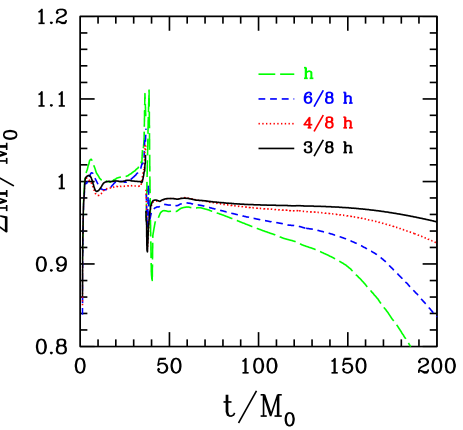
Figure 1: The normalized sum of total AH mass (29) as a function of time, for the head-on collision simulations described in Sec. IV with constraint damping (compare Fig.4). This plot demonstrates convergence to a conserved mass before and after the merger. The “spiky” behavior about the merger point (around $t=37M_{0}$) is due to AH finder problems as discussed in Sec.III.3.

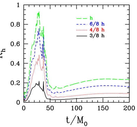
Figure 2: A norm of the residual of the Einstein equations (2), calculated as discussed in Sec. IV.1, for the head-on collision simulations described in Sec. IV with constraint damping (compare Fig.5, though note the different vertical and horizontal scales). This demonstrates the convergence of the solution—see also Fig. 3.

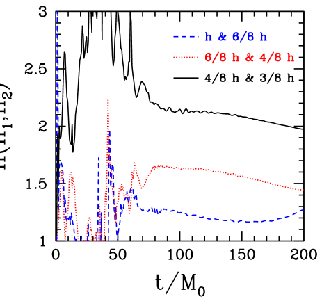
Figure 3: The order of convergence (37) calculated from the head-on collision simulations described in Sec. IV (with constraint damping), and using the residual data shown in Fig. 2. The discretization scheme is second order, and so one would expect $n(h_{1},h_{2})$ to asymptote to 2 as the resolution is increased. This is evident in the figure, particularly after most of the scalar field has left the domain (around $t\approx 40-50M_{0}$).

IV.2 Constraint Damping

This section contains a few results demonstrating the effectiveness of constraint damping. Fig. 4 is the equivalent of Fig. 1, showing the sum of apparent horizon masses as a function of time, though now the corresponding set of simulations have been run with the constraint damping parameter $\kappa=0$. All of the simulations without constraint damping “crashed” before the holes merged, which is why the curves end abruptly. Fig. 5 shows plots of the residual $\mathcal{R}_{h}$ for the simulations without constraint damping—compare to Fig. 2, though note the different scales used in the two plots. This clearly shows how effective constraint damping is, though does not tell us how large $\kappa$ needs to be to start to work. To get an idea for what the required magnitude of $\kappa$ is, a set of $4/8h$ resolution simulations were run with a range of different $\kappa$’s—Fig. 6 shows the residual from these simulations. This demonstrates that $\kappa$ needs to be of order unity (relative to $1/M_{0}$), though no fine tuning is necessary, i.e. there are a range of values $\kappa>\kappa_{0}$ that are all essentially equivalent in damping rapid growth in the constraints.

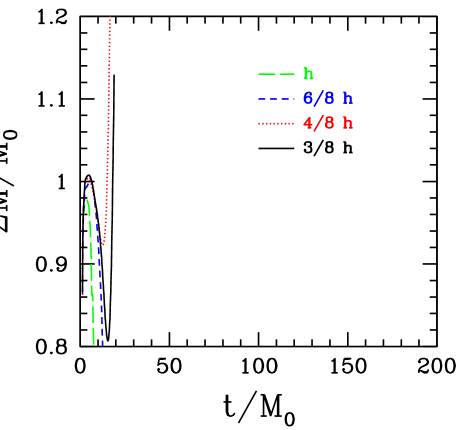
Figure 4: The normalized sum of total AH mass (29) as a function of time, for the head-on collision simulations described in Sec. IV and without constraint damping; compare Fig. 1. The curves end when the simulations crashed.

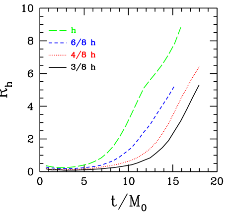
Figure 5: A norm of the residual of the Einstein equations (2), calculated as discussed in Sec. IV.1, for the head-on collision simulations described in Sec. IV without constraint damping; compare Fig.2, though note the different vertical and horizontal scales. Again, convergence is evident, though the rapid growth of the residual with time prevents useful results from being obtained at modest resolution.

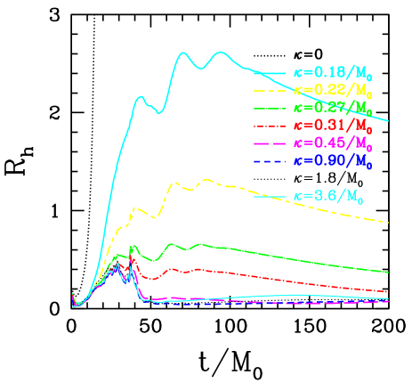
Figure 6: Norms of the residual of the Einstein equations (2), calculated as discussed in Sec. IV.1, for a set of identical “$4h/8$” resolution head-on collision simulations, though with differing values of the constraint damping parameter $\kappa$. The results shown in Fig. 2 were obtained with $\kappa=1.8/M_{0}$ (though note the different vertical scale).

IV.3 Source Function Evolution

Fig. 7 demonstrates the effect of changing parameters in the source function evolution equation (16) for the head-on collision simulation; Table 2 shows the values of the parameters for each set of curves plotted. To avoid clutter in the figure results are given from only 4 different simulations, however these are quite representative of the range of behavior seen with this gauge evolution equation. The figure shows the lapse function $\alpha$ along the axis of symmetry at a few select times (at $t=0$, $\alpha\approx 1$ and is identical in all cases). There are several features shown in the figure worth mentioning. First, the curve ($D$) demonstrates source function evolution without a damping term; this tends to cause oscillations about $1$ in the lapse, and with sufficiently large values of $\xi_{1}$ the oscillations grow to the point where the code crashes. This is the reason the ($D$) curve is not visible at late times.

Second, in cases with a source term ($A$,$C$,$D$) $\alpha$ does not evolve to $1$ in the strong-field regime even at late times, though is closer to $1$ than harmonic gauge ($B$). For example, near merger at $t=29.9M_{0}$ the minimum value $\alpha_{\rm{min}}$ outside the excision surface for harmonic gauge is $\alpha_{\rm{min}}=0.213$ compared to $0.505$ for case $C$, and at $t=200M$ $\alpha_{\rm{min}}=0.458$ (harmonic) versus $0.607$ ($C$). These differences might not seem too significant, and at least for head-on collisions all cases except $D$ work adequately. With non head-on collisions where there is significant orbital motion prior to merger, the small values that the lapse tends to with harmonic gauge seem to be problematic in that instabilities form before a common horizon is detected. There is not convincing evidence that this is coordinate problem as opposed to a numerical issue, though given how “expensive” simulations are in $3D$ and that the non-harmonic gauge works, this issue has not yet been explored in any detail.

Third, notice that for all gauge evolution schemes that are long-time stable ($A,B,C$), at late times the solution approaches a largely time independent form. This gauge condition therefore seems to be “symmetry-seeking”, at least for this class of spacetimes.

	label	$\xi_{1}$	$\xi_{2}$	$\eta$
	A	$0.5/M_{0}^{2}$	$5.4/M_{0}$	$1$
	B	$0$	$0$	$0$
	C	$0.5/M_{0}^{2}$	$5.4/M_{0}$	$7$
	D	$0.5/M_{0}^{2}$	$0$	$1$

Table 2: Values of the parameters in the gauge evolution equation (16) used for the comparison simulation results shown in Fig. 7.

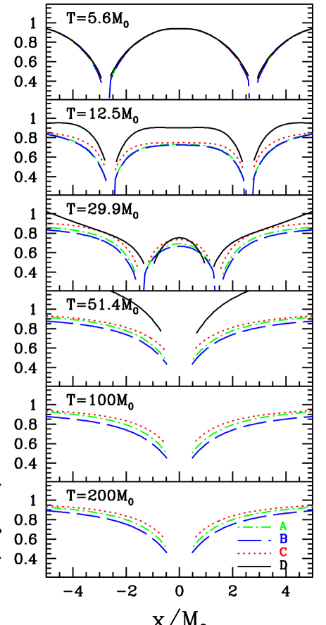
Figure 7: The lapse function $\alpha$ along the axis of symmetry recorded at several times from a set of “$4h/8$” head-on collision simulations as described in Sec. IV, with different parameters in the evolution equation (16) used for $H_{t}$—see Table 2. Case A features the same values as the simulation results shown in Fig.’s 1-6, case B is pure harmonic gauge, case C has a larger $\eta$ coefficient than case A and so is more effective at keeping the lapse closer to $1$, and case D is the same as A though with zero damping coefficient $\xi_{2}$. Without the damping term the driving term, controlled by $\xi_{1}$, is too large in this example, and $\alpha$ overshoots $1$ by a sufficiently large factor that the simulation crashes, which is why curve $D$ is not present in the last two frames.

IV.4 Comparison with 3D evolutions

Here it is demonstrated that some of the results just discussed for the 2D, axisymmetric head-on collisions apply to the full 3D merger problems described in Sec. V, by comparing a select case. Fig. 8 below shows the residual $\mathcal{R}_{h}$ from three 3D simulations with similar grid structure to the three lowest resolution 2D results shown in Fig. 2; the sum of AH masses with time is shown in Fig. 9; and though there is no direct comparison to the 2D results Fig. 10 shows the estimated Kerr spin parameter $a$ after the merger. The parameters for the 3D simulations were chosen so that the equal mass merger occurs in roughly an orbit and a half for each resolution—see Fig. 11. Note that the boost parameters differ slightly for each resolution; this, as discussed in Sec.V, is due to the sensitivity of the resultant orbit to the initial data parameters. Of course, in the continuum limit one would expect convergence to a definite orbit for a given boost parameter, or conversely, given a desired orbit the required boost parameter should converge to a definite value. However, what Fig. 8 is meant to show is the behavior of the residual $\mathcal{R}_{h}$ with time and as resolution varies, and so for a meaningful comparison simulations with similar grid structures and run-times were used.

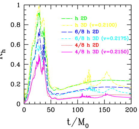
Figure 8: Comparison plots of the norm of the residual of the Einstein equations (2), calculated as discussed in Sec. IV.1, between the head-on collision simulations described in Sec. IV (labeled $2D$—see Fig.2) and non head-on mergers (labeled $3D$) as discussed in Sec. V. $3h/8$ resolution simulations were not run in 3D due to lack of computational resources. Note also that the momentary increase in the residual near $t=100M_{0}-150M_{0}$ in the $3D$ simulations is around the time of merger.

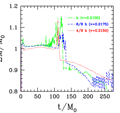
Figure 9: The normalized sum of total AH mass (29) as a function of time for 3 merger simulations (see Fig.11), as described in Sec. V. In each case the boost parameter was chosen so that roughly one and a half orbits is completed before merger, to better facilitate the comparison of the effect of resolution on solution accuracy (see the discussion in Sec. V). The late-time problems with the AH finder for the $6h/8$ case seems to set in when numerical error causes the angular momentum of the black hole to approach extremality–see Fig. 10.

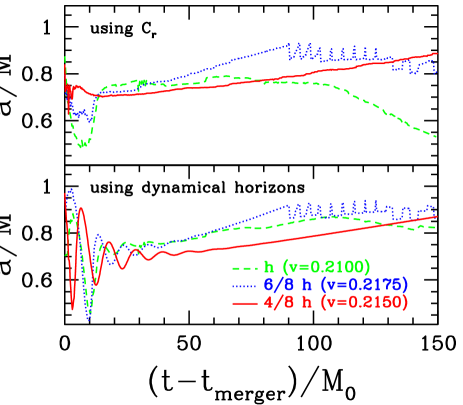
Figure 10: Estimates of the angular momentum of the final black hole, corresponding to the simulations shown in Fig.’s 9 and 11, calculated using (30) and the dynamical horizons framework in the top and bottom plots respectively. To facilitate the comparison the time has been shifted so that $t=0$ corresponds to the moment an encompassing AH is first detected. Note that with increased resolution the drift in $a/M$ decreases at late times, as to be expected in a convergent solution. The $6h/8$ resolution case demonstrates what is seemingly a further source of robustness problems in the AH finder when the angular momentum approaches extremality (the spin-up is numerical-error driven here).

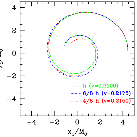
Figure 11: A plot of the orbits of the $3D$ simulations used to compare with the head-on collision results (Fig. 8). What is shown for each case is the coordinate position of the center of the apparent horizon of one of the black holes.

V Scalar Field Collapse Driven Binary Black Hole Spacetimes

In this section some results are presented from an ongoing study of scalar field collapse driven black hole merger simulations. The disadvantages of this approach to constructing an orbit, from the point of view of simulating astrophysically relevant binary configurations, is that one does not have a priori control over the orbit that will result, and perhaps more problematic is that in the regime where the evolution is started the radiation-reaction is sufficiently strong that it is not easy to deduce an astrophysical orbit that the binary might have evolved from. Therefore, these binary might be in a region of parameter space that are not shared by astrophysical systems. However, from a theoretical perspective of trying to understand the dynamics of binary black hole coalescence in general relativity, this scalar field collapse initial data is a straight-forward and simple way to probe a large and interesting region of parameter space.

Here the focus will be on one particular family of initial conditions: identical initial scalar field distributions ($A=0.3$ and $\Delta=0.827M_{0}$) except that one is located at $(x,y,z)=(4.45M_{0},0,0)$ and given a boost with boost parameter $v$ in the positive-$y$ direction, while the other is located at $(x,y,z)=(-4.45M_{0},0,0)$ and given a boost $v$ in the negative-$y$ direction—see (28) and the discussion afterwards. Approximately $85\%$ of the energy in the scalar field falls into the black holes that form, while the remaining energy radiates away on roughly an orbital light-crossing time scale.

This choice of initial data gives a single parameter $v$ that can be varied. The black holes are initially sufficiently far apart—a coordinate (proper) separation of $8.90M_{0}$ ($10.8M_{0}$)—that with a large enough boost parameter one would expect the system to be unbound. At the other extreme, $v=0$ will give a head on collision. Thus there is a range of values $0\leq v_{c}$ for some $v=v_{c}$ that will result in a merger, and it is this region of parameter space we want to explore. For the purposes of studying the gravitational radiation produced by mergers, and in particular comparing the orbital to plunge and ringdown part of the waves, it is useful to have parameters that result in several orbits before the merger–see 12 for a plot of the orbit from one such parameter. This regime is where these BBH simulations become quite interesting, in that there is apparently extreme sensitivity of the solution as a function of the boost parameter. In particular, the dependence of the number of orbits $n$ as a function of $v$, $n(v)$ is quite reminiscent of certain aspects of critical phenomena in gravitational collapse in that there are apparently two distinct end states, merger of the black holes for $v<v^{\star}$ versus separation for $v>v^{\star}$, and the closer $v$ is to $v^{\star}$ the more orbits before merger/separation that are observed —see Table 3 below for data from several simulations, Fig. 13 for a plot of the orbits from two of the $6/8h$ resolution runs that have been fine-tuned the most to date, and Fig. 14 for graphs of the corresponding gravitational waves emitted. This behavior is also quite reminiscent of “zoom-whirl” orbits seen in the trajectories of point-particle orbits about black holeszoom_whirl , and might simply be the fully non-linear equivalent of the zoom-whirl phenomena. In fact, for zoom-whirl particle orbits there is exponential sensitivity of the number of orbits $N_{w}$ completed in each whirl phase to the initial conditions : $p-p_{s}=e^{-aN_{w}}$, where $p$ is the semi-latus rectum of the orbit, $p_{s}$ is the separatrix of bound orbits, and $a$ is some constant that depends (amongst other things) on the eccentricity of the orbit and spin of the central black holezoom_whirl_b . Of course, in the full solution where energy is lost through gravitational wave emission $N_{w}$ can not be arbitrarily large. Furthermore, $v^{\star}$ loosely defined above cannot be a “true” boundary between merger and separation, for one would still expect the orbits to be bound for $v$ slightly greater than $v^{*}$—the binary will just “whirl” out some distance before later merging.

Note that the sensitivity to initial conditions complicates convergence testing (i.e. verification) of this interesting indication that zoom-whirl like behavior is present in equal mass binary merger spacetimes. This is because sensitivity to initial conditions implies that the “bifurcate” regime of parameter space must be found independently using several resolutions; i.e. one cannot do a “quick” low-resolution search to find $v\approx v^{\star}$, then perform a high resolution simulation to verify the low-resolution result, as each resolution will have a different $v^{\star}$. Furthermore, the numerical error that accumulates per orbit, as judged using AH mass conservation, is relatively large, in particular for the lower resolution simulations, where the AH mass changes by a few percent per orbit. This is larger that the energy lost through gravitational wave emission, and though it does not exactly make sense to equate numerical error with physical energy, that these two “effects” are of the same order of magnitude suggests one cannot yet draw significant conclusions from these early results.

h-resolution runs
$v$ $n$ $p_{m}/M_{0}$ $d_{m}/M_{0}$ $m_{f}/M_{0}$ $a/m_{f}$ $(E/M_{0})$ $0.21000$ $1.3$ $-$ $-$ $0.89\pm 0.03$ $0.75\pm 0.05$ $0.032$ $0.21125$ $1.4$ $-$ $-$ $0.88\pm 0.03$ $0.74\pm 0.05$ $0.035$ $0.21234$ $2.3$ $-$ $-$ $0.83\pm 0.03$ $0.73\pm 0.05$ $?$ $0.21250$ $2.7$ $4.0$ $3.6$ $-$ $-$ $0.020$ $0.21500$ $1.5$ $5.5$ $4.6$ $-$ $-$ $0.006$ $0.22000$ $1.0$ $7.2$ $5.8$ $-$ $-$ $0.005$

6/8 h-resolution runs
$v$ $n$ $p_{m}/M_{0}$ $d_{m}/M_{0}$ $m_{f}/M_{0}$ $a/m_{f}$ $(E/M_{0})$ $0.20960$ $0.9$ $-$ $-$ $0.97\pm 0.01$ $0.65\pm 0.03$ $0.028$ $0.21750$ $1.4$ $-$ $-$ $0.92\pm 0.01$ $0.72\pm 0.03$ $0.037$ $0.21875$ $2.0$ $-$ $-$ $0.88\pm 0.01$ $0.70\pm 0.03$ $0.046$ $0.21906$ $2.4$ $-$ $-$ $0.86\pm 0.01$ $0.70\pm 0.03$ $0.052$ $0.219180$ $2.8$ $-$ $-$ $0.82\pm 0.02$ $0.70\pm 0.05$ $0.063$ $0.219200$ $3.0$ $-$ $-$ $0.80\pm 0.02$ $0.75\pm 0.05$ $0.064$ $0.219209$ $3.3$ $-$ $-$ $0.78\pm 0.02$ $0.71\pm 0.05$ $0.067$ $0.219214$ $3.7$ $-$ $-$ $0.75\pm 0.02$ $0.71\pm 0.05$ $0.074$ $0.2192175$ $3.9$ $-$ $-$ $0.74\pm 0.02$ $0.70\pm 0.05$ $0.076$ $0.2192181$ $4.3$ $-$ $-$ $0.73\pm 0.02$ $0.71\pm 0.05$ $0.079$ $0.2192188$ $4.9$ $3.2$ $3.0$ $-$ $-$ $0.058$ $0.21938$ $2.5$ $4.8$ $4.2$ $-$ $-$ $0.019$ $0.22000$ $1.9$ $5.3$ $4.4$ $-$ $-$ $0.014$

4/8 h-resolution runs
$v$ $n$ $p_{m}/M_{0}$ $d_{m}/M_{0}$ $m_{f}/M_{0}$ $a/m_{f}$ $(E/M_{0})$ $0.21500$ $1.4$ $-$ $-$ $0.945\pm 0.005$ $0.71\pm 0.02$ 0.042 $0.22000$ $2.1$ $5.7$ $4.8$ $-$ $-$ $0.008$

Table 3: Information extracted from the scalar field collapse driven binary simulations run to-date, described in Sec. V. Results from three different resolutions (see Table 1) are shown (data from the $h$ resolution $v=0.21234$ run was lost, preventing the calculation of $E$ in that case). $v$ is the boost parameter for the initial scalar field pulses and $n$ the number of orbits completed either before a merger, or at the moment the binaries reached the same coordinate separation as at $t=0$. For binaries that did not merge, $p_{m}$ is the minimum proper separation measured at $t={\rm const.}$ along the coordinate line between, though exterior to the AH’s, and $d_{m}$ is the minimum coordinate distance between the coordinate centers of the AH’s. For binaries that merged, the final mass and angular momentum of the black holes, as estimated from AH properties, is listed. $E$ is the total energy emitted in gravitational waves, calculated as described in Sec. III.1 at a coordinate radius of $50M_{0}$ from the origin. Note that the quoted uncertainties in the final BH properties only include an estimated uncertainty from looking at plots such as Fig. 9 and 10. To obtain an estimate of the numerical errors, one can use the Richardson expansion. For example by comparing the $n=1.4$ results between the $6/8h$ and $4/8h$ runs, and using (38), the estimated errors in the $v=0.21500$ $4/8h$ simulation are: $m_{f}=0.95\pm 0.02M_{0}$, $a=0.71\pm 0.01$ and $E=0.042\pm.004$. Once a larger set of simulations have been completed at higher resolution a more thorough analysis of numerical errors will be performed.

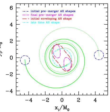
Figure 12: A plot of the orbit of the $v=0.21906$, $6h/8$-resolution merger simulation. The spiral trajectories are the coordinate positions of the centers of the apparent horizons of the two black holes before merger, and the labeled curves show the coordinate shapes of the AH’s, in the $z=0$ plane, at select times.

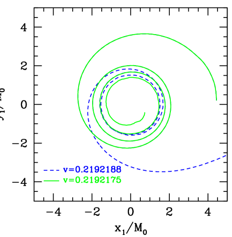
Figure 13: A plot of the orbits of two of the $6h/8$-resolution simulations that have been tuned closest to the bifurcate-like point in boost-parameter space (see Table 3). The merger case orbit ends when an encompassing AH is detected.

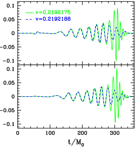
Figure 14: Gravitational waveforms from the two simulations depicted in Fig. 13. What is shown here are the two polarizations of one of the dominant spin weight $-2$ spherical harmonic components of $\Psi_{4}$ (32), calculated over a coordinate sphere a distance $r=50M_{0}$ from the origin, and normalized by $rM_{0}$.

VI Conclusions

In this paper further details were given of the generalized harmonic evolution scheme introduced in paper1 and shown to be capable of simulating binary black hole coalescencepaper2 . In particular, topics included were a demonstration of the effectiveness of constraint damping in a fully non-linear setting, examples of the effect of source function evolution on the time slicing of the spacetime, a discussion of certain technical aspects of the code and problems with the robustness of the apparent horizon finder, and some results from an ongoing study of scalar field collapse driven black hole binary simulations. There are many outstanding issues that need to be explored, including the applicability of constraint damping to more general scenarios and alternative evolution schemes, gaining more evidence for (or against) the zoom-whirl type behavior seen here, studying a broader range of binary black hole merger initial conditions, investigating a larger class of source function evolution equations (in particular to include non-trivial spatial source functions), and beginning to extract some information from the non-perturbative regime of the merger to aid in gravitational wave detection efforts. The scalar field driven binaries are arguably not too useful in regards to this latter point, primarily because of the difficulty in mapping the resulting binary to (some approximation of) an astrophysical binary. Nevertheless, general features of the waveforms could be studied. Furthermore, what these simulations suggest is that to eventually obtain accurate waveforms in the most interesting cases will require significantly improved accuracy in the simulations. Given that the present simulations already utilize significant computer resources, rather than increase the resolution a more realistic near term solution would be to incorporate higher-order finite difference techniques or spectral methods (utb ; utb2 already use fourth order differencing in space and time, and nasa ; nasa2 use fourth order in space and second order in time). Modulo the accuracy issues, numerical relativity finally seems to have entered the era where it will begin uncover what will hopefully be the very rich and interesting landscape of black hole interactions.

Acknowledgments: FP gratefully acknowledges research support from CIAR. The simulations described here were performed on the University of British Columbia’s vnp4 cluster (supported by CFI and BCKDF), WestGrid machines (supported by CFI, ASRI and BCKDF), and Dell Lonestar cluster at the University of Texas in Austin.

References

- (1) F. Pretorius, “Evolution of Binary Black Hole Spacetimes”, Phys. Rev. Lett.95, 121101 (2005)
- (2) M. Campanelli, C.O. Lousto, P. Marronetti and Y. Zlochower, “Accurate Evolutions of Orbiting Black-Hole Binaries Without Excision”, Phys. Rev. Lett.96, 111101 (2006)
- (3) J. G. Baker, J. Centrella, D. Choi, M. Koppitz and J. van Meter, “Gravitational Wave Extraction from an Inspiraling Configuration of Merging Black Holes”, Phys. Rev. Lett.96, 111102 (2006)
- (4) T. Nakamura, K. Oohara and Y. Kojima, Prog. Theor. Phys. Suppl. 90, 1 (1987)
- (5) M. Shibata and T. Nakamura, “Evolution of three-dimensional gravitational waves: Harmonic slicing case”, Phys. Rev. D52, 5428 (1995).
- (6) T. W. Baumgarte and S.L. Shapiro, “Numerical integration of Einstein’s field equations”, Phys. Rev. D59, 024007 (1999)
- (7) M. Campanelli, C.O. Lousto and Y. Zlochower, “The Last Orbit of Binary Black Holes”, Phys. Rev. D73, 061501 (2006)
- (8) J. G. Baker, J. Centrella, D. Choi, M. Koppitz and J. van Meter, “Binary Black Hole Merger Dynamics and Waveforms”, Phys. Rev. D73, 104002 (2006)
- (9) F. Herrmann, D. Shoemaker and P. Laguna, “Unequal-Mass Binary Black Hole Inspirals”, gr-qc/0601026 (2006)
- (10) J. G. Baker, J. Centrella, D. Choi, M. Koppitz, J. van Meter and M. Coleman Miller, “Getting a kick out of numerical relativity”, astro-ph/0603204 (2006)
- (11) M. Campanelli, C.O. Lousto and Y. Zlochower, “Gravitational radiation from spinning-black-hole binaries: The orbital hang up”, gr-qc/0604012 (2006)
- (12) B. Brugmann, “Binary Black Hole Mergers in 3d Numerical Relativity,” Int. J. Mod. Phys. D 8, 85 (1999)
- (13) B. Bruegmann, W. Tichy and N. Jansen “Numerical simulation of orbiting black holes”, Phys.Rev.Lett. 92 211101, (2004)
- (14) F. Pretorius, “Numerical Relativity Using a Generalized Harmonic Decomposition”, Class. Quant. Grav. 22 425, (2005)
- (15) L. Lindblom, M. A. Scheel, L. E. Kidder, R. Owen and O. Rinne, “A New Generalized Harmonic Evolution System”, gr-qc/0512093 (2005)
- (16) G. B. Cook and H. P. Pfeiffer, “Excision boundary conditions for black hole initial data,” Phys. Rev. D 70, 104016 (2004)
- (17) A. Buonanno, G. Cook and F. Pretorius, in preparation
- (18) D. Garfinkle, “Harmonic coordinate method for simulating generic singularities”, Phys.Rev. D65, 044029 (2002)
- (19) B. Szilagyi, B. G. Schmidt and J. Winicour, “Boundary conditions in linearized harmonic gravity,” Phys. Rev. D 65, 064015 (2002)
- (20) B. Szilagyi and J. Winicour, “Well-Posed Initial-Boundary Evolution in General Relativity”, Phys.Rev. D68, 041501 (2003)
- (21) M. C. Babiuc, B. Szilagyi and J. Winicour, “Testing numerical relativity with the shifted gauge wave,” gr-qc/0511154 (2005)
- (22) M. C. Babiuc, B. Szilagyi and J. Winicour, “Harmonic Initial-Boundary Evolution in General Relativity,” Phys.Rev. D73, 064017 (2006)
- (23) C. Gundlach, J. M. Martin-Garcia, G. Calabrese and I. Hinder, “Constraint damping in the Z4 formulation and harmonic gauge,” Class. Quant. Grav. 22, 3767 (2005).
- (24) O. Brodbeck, S. Frittelli, P. Hubner and O. A. Reula, “Einstein’s equations with asymptotically stable constraint propagation,” J. Math. Phys. 40, 909 (1999)
- (25) C. Bona, T. Ledvinka, C. Palenzuela and M. Zacek, “General-covariant evolution formalism for Numerical Relativity”, Phys. Rev. D67, 104005 (2003)
- (26) H. Friedrich, “Hyperbolic reductions for Einstein’s equations”, Class. Quant. Grav. 13, 1451 (1996)
- (27) J. Balakrishna, G. Daues, E. Seidel, W. Suen, M. Tobias, E. Wang, “Coordinate Conditions and Their Implementation in 3D Numerical Relativity”, Class. Quant. Grav. 13, L135 (1996)
- (28) M. Alcubierre, B. Bruegmann, P. Diener, M. Koppitz, D. Pollney, E. Seidel, R. Takahashi, “Gauge conditions for long-term numerical black hole evolutions without excision”, Phys. Rev. D67, 084023 (2003)
- (29) L. Lindblom and M.A. Scheel, “Dynamical Gauge Conditions for the Einstein Evolution Equations”, Phys. Rev. D67, 124005 (2003)
- (30) M. Alcubierre, A. Corichi, J. A. Gonzalez, D. Nunez, B. Reimann and M. Salgado, “Generalized harmonic spatial coordinates and hyperbolic shift conditions,” Phys. Rev. D 72, 124018 (2005)
- (31) C. Bona, J. Carot and C. Palenzuela-Luque, “Almost-stationary motions and gauge conditions in general relativity,” Phys. Rev. D 72, 124010 (2005)
- (32) C. Bona, L. Lehner and C. Palenzuela-Luque, “Geometrically motivated hyperbolic coordinate conditions for numerical relativity: Analysis, issues and implementations,” Phys. Rev. D 72, 104009 (2005)
- (33) G. B. Cook, “Initial Data for Numerical Relativity”, Living Rev.Rel. 3, 5 (2000)
- (34) R. Arnowitt, S. Deser and C.W. Misner, in Gravitation: An Introduction to Current Research, ed. L. Witten, New York, Wiley (1962)
- (35) H. Friedrich, “On the Hyperbolicity of Einstein’s and Other Gauge Field Equations”, Commun. Math. Phys 100, 525 (1985)
- (36) PAMR (Parallel Adaptive Mesh Refinement) and AMRD (Adaptive Mesh Refinement Driver) libraries (http://laplace.physics.ubc.ca/Group/Software.html)
- (37) G. Calabrese, “Finite differencing second order systems describing black hole spacetimes”, Phys. Rev. D 71, 027501 (2005)
- (38) A. Ashtekar and B. Krishnan “Isolated and dynamical horizons and their applications,” Living Rev. Rel. 7, 10 (2004)
- (39) S.R. Brandt and E. Seidel, “The Evolution of Distorted Rotating Black Holes II: Dynamics and Analysis”, Phys.Rev. D52, 870 (1995)
- (40) A. Nerozzi, C. Beetle, M. Bruni, L. M. Burko and D. Pollney, “Towards wave extraction in numerical relativity: The quasi-Kinnersley frame,” Phys. Rev. D 72, 024014 (2005)
- (41) L. Smarr, in Sources of Gravitational Radiation, ed. L. Smarr, Seattle, Cambridge University Press (1978)
- (42) J. Thornburg, “Finding Apparent Horizons in Numerical Relativity”, Phys. Rev. D54, 4899 (1996)
- (43) J. Thornburg, “Event and Apparent Horizon Finders for Numerical Relativity,” gr-qc/0512169 (2005)
- (44) C. Cutler, D. Kennefick and E. Poisson, “Gravitational radiation reaction for bound motion around a Schwarzschild black hole,” Phys. Rev. D 50, 3816 (1994).
- (45) K. Glampedakis and D. Kennefick, “Zoom and whirl: Eccentric equatorial orbits around spinning black holes and their evolution under gravitational radiation reaction,” Phys. Rev. D 66, 044002 (2002)