Reducing orbital eccentricity in initial data of binary neutron stars

Abstract

We develop a method to compute low-eccentricity initial data of binary neutron stars required to perform realistic simulations in numerical relativity. The orbital eccentricity is controlled by adjusting the orbital angular velocity of a binary and incorporating an approaching relative velocity of the neutron stars. These modifications improve the solution primarily through the hydrostatic equilibrium equation for the binary initial data. The orbital angular velocity and approaching velocity of initial data are updated iteratively by performing time evolutions over $\sim$ 3 orbits. We find that the eccentricity can be reduced by an order of magnitude compared to standard quasicircular initial data, specifically from $\sim$ 0.01 to $\lesssim$ 0.001, by three successive iterations for equal-mass binaries leaving $\sim$ 10 orbits before the merger.

I Introduction

Fully general relativistic simulations of binary neutron star mergers have been extensively performed in the past fifteen years (see Ref. faber_rasio2011 and reference therein for earlier works). Prime targets of these studies are initially circular binaries with irrotational velocity fields, because gravitational radiation reaction circularizes most of the binaries before they enter sensitive bands of ground-based gravitational-wave detectors peters1964 and the viscosity of neutron-star matter is expected to be too low to significantly increase the neutron-star spin via tidal effects kochanek1992 ; bildsten_cutler1992 . In addition, the orbital period of binary neutron stars right before the merger is much smaller than typical rotational periods of observed neutron stars lorimer2008 . Numerical-relativity simulations of binary neutron stars have elucidated quantitatively the formation of remnant massive neutron stars and/or collapse to black hole-disk systems hotokezaka_kkmsst2013 ; hotokezaka_kss , substantial mass ejection hotokezaka_kkosst2013 , and gravitational waveforms during the inspiral-merger-postmerger phases hotokezaka_ks2013 ; read_bcfgkmrst2013 .

All the simulations of “circular” binary neutron stars have suffered from unphysical orbital eccentricity. To perform numerical simulations of circular binary neutron stars throughout inspiral, merger, and postmerger phases, sufficiently circularized initial data are necessary. To date, quasiequilibrium states, which are solutions to a subset of the Einstein equations and hydrostatics under physical assumptions gourgoulhon_gtmb2001 ; taniguchi_gourgoulhon2002 ; taniguchi_gourgoulhon2003 ; taniguchi_shibata2010 , have usually been adopted as initial data of numerical simulations. Although the formulation for irrotational velocity fields has been developed to a satisfactory level bonazzola_gm1997 ; asada1998 ; shibata1998 ; teukolsky1998 , it has failed to give sufficiently circularized binaries and instead has resulted in eccentricities $e\gtrsim 0.01$. Computations of quasicircular binary neutron stars have been carried out assuming the existence of a helical Killing vector field with the orbital angular velocity $\Omega$. Because this formulation neglects the gravitational radiation reaction and does not appropriately incorporate the approaching velocity, a binary prepared in this manner evolves as a slightly but appreciably eccentric binary once a numerical simulation is launched. Some effort has been made to remove the eccentricity by adding a post-Newton-inspired approaching velocity to quasicircular initial data kiuchi_sst2009 or by constraint-violating superposition of Lorentz-boosted stationary stars tsatsin_marronetti2013 , but the eccentricity is not reduced below $e\sim 0.01$.

Reducing the orbital eccentricity is an urgent task in numerical relativity, and the most important reason for this is high demand to derive accurate gravitational waveforms. Although mismatch due to the orbital eccentricity in quasicircular initial data is reported to be merely $\sim$ 1% in binary black hole simulations if we focus only on the numerical-relativity waveforms pfeiffer_bklls2007 , the eccentricity complicates comparisons between gravitational waveforms obtained by numerical simulations and those derived by analytic methods both for binary black holes buonanno_cp2007 ; boyle_bkmpsct2007 ; hannam_hgsb2008 and binary neutron stars baiotti_dgnr2011 ; bernuzzi_ntb2012 ; hotokezaka_ks2013 . The eccentricity also affects hybridization of analytic and numerical waveforms, which is necessary to create phenomenological templates covering a wide frequency domain (see Refs. lackey_ksbf2012 ; pannarale_bks2013 ; foucart_ddkmopsst2013 ; lackey_ksbf2014 for relevant works of black hole-neutron star binaries). The extraction of tidal deformability from gravitational waves is fairly sensitive to the accuracy of templates favata2014 ; yagi_yunes2014 ; wade_colflr2014 , and thus reducing the orbital eccentricity is critical to maximizing the precision with which we can extract neutron-star parameters and constrain the neutron-star equations of state from gravitational-wave observations.

In this paper, we describe a method to reduce orbital eccentricity in initial data of binary neutron stars. The basic idea is similar to that of eccentricity reduction for binary black holes pfeiffer_bklls2007 . Namely, we correct initial data using their orbital evolution obtained by dynamical simulations and repeat this procedure until a desired value of the orbital eccentricity is achieved. Specifically, we adjust the orbital angular velocity and incorporate an approaching velocity. The primary difference from the binary black hole cases resides in the method for computing initial data of binary neutron stars with an approaching velocity. In binary black hole problems solved in the extended conformal thin-sandwich formulation (see Sec. II), the approaching velocity and eccentricity of initial data are controlled via inner boundary conditions imposed at black hole horizons pfeiffer_bklls2007 . Instead, we control them by modifying hydrostatics of neutron stars. As a first attempt to reduce the orbital eccentricity in binary neutron stars, we aim for eccentricity lower than $\sim 0.001$, which satisfies the requirement $e\lesssim 0.002$ of the Numerical-Relativity and Analytical-Relativity Collaboration for binary black holes hinder_etal2014 .

This paper is organized as follows. In Sec. II, we describe our method to compute low-eccentricity initial data of binary neutron stars with an approaching velocity. A procedure to analyze orbital evolution is presented in Sec. III with a brief description of our simulation code, including an update from the Baumgarte–Shapiro–Shibata–Nakamura (BSSN) formulation shibata_nakamura1995 ; baumgarte_shapiro1998 to conformally decomposed Z4 (Z4c) formulation bernuzzi_hilditch2010 . Actual eccentricity reduction and results obtained with low-eccentricity initial data are demonstrated in Sec. IV. Section V is devoted to a summary and discussions.

Greek and Latin indices denote the spacetime and space components, respectively. Geometrical units in which $G=c=1$, where $G$ and $c$ are the gravitational constant and speed of light, respectively, are adopted throughout this paper.

II Initial data computation

We compute initial data of binary neutron stars in the extended conformal thin-sandwich formulation york1999 ; pfeiffer_york2003 . We also solve equations of hydrostatics to obtain quasiequilibrium fluid configurations. The formulation is formally very similar to that for quasicircular initial data, for which the details are found in Refs. gourgoulhon_gtmb2001 ; taniguchi_gourgoulhon2002 ; taniguchi_gourgoulhon2003 ; taniguchi_shibata2010 . All the numerical computations of initial data are performed with a public multidomain spectral method library, LORENE LORENE , and numerical details are found in Refs. bonazzola_gm1998 ; gourgoulhon_gtmb2001 .

II.1 Gravitational field equations

Physically valid initial data have to satisfy the Hamiltonian and momentum constraints at the very least, and some quasiequilibrium assumptions are desired to be met for astrophysically realistic binary initial data. In this study, we compute initial data of the induced metric $\gamma_{ij}$ and extrinsic curvature $K_{ij}$ in the extended conformal thin-sandwich formulation york1999 ; pfeiffer_york2003 . A conformal transformation is defined by

$$\gamma_{ij} =\psi^{4}\hat{\gamma}_{ij}\;,\;\gamma^{ij}=\psi^{-4}\hat{\gamma}_{ij},$$ (1)

$$A^{ij} =\psi^{-10}\hat{A}^{ij}\;,\;A_{ij}=\psi^{-2}\hat{A}_{ij},$$ (2)

where $A_{ij}$ is the traceless part of the extrinsic curvature given as

$$A_{ij}\equiv K_{ij}-\frac{1}{3}K\gamma_{ij}\;,\;K\equiv\gamma^{ij}K_{ij}.$$ (3)

We handle a weighted lapse function $\Phi\equiv\alpha\psi$ instead of the lapse function $\alpha$ itself in the computation of initial data for the sake of numerical accuracy, whereas the shift vector $\beta^{i}$ is handled as it is. A traceless evolution tensor of the conformal induced metric,

$$\hat{u}_{ij}=\partial_{t}\hat{\gamma}_{ij},$$ (4)

with $\hat{\gamma}^{ij}\hat{u}_{ij}=0$ is also introduced as freely specifiable data in this formulation.

To obtain a quasiequilibrium configuration of binary neutron stars, we impose conditions,

$$\hat{\gamma}_{ij}=f_{ij}\;,\;K=0\;,\;\hat{u}_{ij}=0\;,\;\partial_{t}K=0,$$ (5)

on freely specifiable data. Here, $f_{ij}$ is the flat 3-metric. In principle, attention has to be paid for the frame in which equations are solved, since the latter two stationarity conditions could be imposed even approximately only when the time direction is chosen to agree with the binary motion. Specifically, the change of frames amounts to adopting different shift vectors, which appears in various terms of gravitational field equations. It turns out that, however, the equations are unaffected by the addition of a reasonable approaching velocity as pointed out in Ref. pfeiffer_bklls2007 . The reason for this is that the difference of the shift vector enters the equations only through (i) the conformal Killing operator associated with $\hat{\gamma}_{ij}$ and (ii) the Lie derivative of $K$. This is the very reason why a rotational shift vector of the form $\Omega\left(\partial_{\varphi}\right)^{\mu}$ has not appeared explicitly in the computation of quasicircular initial data gourgoulhon_gtmb2001 ; taniguchi_gourgoulhon2002 ; taniguchi_gourgoulhon2003 ; taniguchi_shibata2010 .

One plausible way to incorporate an approaching velocity may be to add uniform contraction to the helical Killing vector in the manner pfeiffer_bklls2007

$$\xi^{\mu}=\left(\partial_{t}\right)^{\mu}+\Omega\left(\partial_{\varphi}\right)^{\mu}+v\frac{r}{r_{0}}\left(\partial_{r}\right)^{\mu}$$ (6)

and impose the quasiequilibrium conditions, Eq. (5), in the time direction given by $\xi^{\mu}$ [see also Eq. (20)]. Here, $v$ (negative for the approaching velocity) and $r_{0}$ should be regarded as the radial velocity and separation from the coordinate origin, respectively, averaged over binary members. For an equal-mass binary, $v$ and $r_{0}$ should be common in each member, and the averaging is not required. The radial velocity term $r(\partial_{r})^{i}$ is a conformal Killing vector of the flat metric, and hence this term does not affect gravitational field equations. The boundary condition of the shift vector (see below) is also unaffected, because a conformal Killing vector is a homogeneous solution of the vectorial Laplacian.

The equations to be solved for gravitational fields become taniguchi_shibata2010

$${\raise 4.30554pt\hbox{${}^{\,\circ}$}}\!\!\!\!D^{2}\psi =-\frac{1}{8}\psi^{-7}\hat{A}_{ij}\hat{A}^{ij}-2\pi\psi^{5}\rho_{\mathrm{H}},$$ (7)

$${\raise 4.30554pt\hbox{${}^{\,\circ}$}}\!\!\!\!D^{2}\beta^{i}+\frac{1}{3}{\raise 4.30554pt\hbox{${}^{\,\circ}$}}\!\!\!\!D^{i}{\raise 4.30554pt\hbox{${}^{\,\circ}$}}\!\!\!\!D_{j}\beta^{j} =2\hat{A}^{ij}{\raise 4.30554pt\hbox{${}^{\,\circ}$}}\!\!\!\!D_{j}\left(\Phi\psi^{-7}\right)+16\pi\Phi\psi^{3}j^{i},$$ (8)

$${\raise 4.30554pt\hbox{${}^{\,\circ}$}}\!\!\!\!D^{2}\Phi =\frac{7}{8}\Phi\psi^{-8}\hat{A}_{ij}\hat{A}^{ij}+2\pi\Phi\psi^{4}\left(\rho_{\mathrm{H}}+2S\right),$$ (9)

$$\hat{A}^{ij} =\frac{\psi^{7}}{2\Phi}\left({\raise 4.30554pt\hbox{${}^{\,\circ}$}}\!\!\!\!D^{i}\beta^{j}+{\raise 4.30554pt\hbox{${}^{\,\circ}$}}\!\!\!\!D^{j}\beta^{i}-\frac{2}{3}f^{ij}{\raise 4.30554pt\hbox{${}^{\,\circ}$}}\!\!\!\!D_{k}\beta^{k}\right),$$ (10)

where ${\raise 4.30554pt\hbox{${}^{\,\circ}$}}\!\!\!\!D_{i}$ is the covariant derivative associated with the flat metric, $f_{ij}$. The matter source terms are defined from the 3+1 decomposition of the energy-momentum tensor $T_{\mu\nu}$ in terms of a future-directed unit normal vector $n^{\mu}$ to the constant-time hypersurface as

$$\rho_{\mathrm{H}} =T_{\mu\nu}n^{\mu}n^{\nu},$$ (11)

$$j_{i} =-\gamma_{i\mu}T^{\mu\nu}n_{\nu},$$ (12)

$$S_{ij} =\gamma_{i\mu}\gamma_{j\nu}T^{\mu\nu}.$$ (13)

The scalar elliptic equations are solved with boundary conditions,

$$\psi,\Phi\to 1\;(r\to\infty),$$ (14)

derived from the asymptotic flatness. The boundary condition on the shift vector determines the frame in which the equations are solved, and we can simply set

$$\beta^{i}\to 0\;(r\to\infty),$$ (15)

according to the discussion above, remembering that $\beta^{i}$ obtained with this is that for an asymptotically inertial frame.

II.2 Hydrostatics

The neutron-star matter is modeled by a perfect fluid with zero temperature, for which all the thermodynamic quantities are given as functions of only one representative, in our computation of initial data. The energy-momentum tensor takes the form

$$T_{\mu\nu}=\rho hu_{\mu}u_{\nu}+Pg_{\mu\nu},$$ (16)

where $\rho$, $P$, $h$, and $u^{\mu}$ are the rest-mass density, pressure, specific enthalpy, and 4-velocity of the fluid, respectively. The specific enthalpy is defined by $h=1+\varepsilon+P/\rho$, where $\varepsilon$ is the specific internal energy. The hydrodynamic equations comprise the continuity equation

$$\nabla_{\mu}\left(\rho u^{\mu}\right)=0$$ (17)

and the local energy-momentum conservation equation

$$\nabla_{\nu}T^{\mu\nu}=0,$$ (18)

where $\nabla_{\mu}$ is the covariant derivative associated with the spacetime metric. Because we focus only on the irrotational velocity field, a velocity potential $\Psi$ such that

$$\nabla_{\mu}\Psi=hu_{\mu}$$ (19)

can be introduced shibata1998 ; teukolsky1998 . The time component of Eq. (18) in the comoving frame of the fluid merely gives Eq. (17) for a zero-temperature perfect fluid, and the spatial components of Eq. (18), or the relativistic Euler equation, are shown to be integrable for an irrotational flow in the presence of symmetry shibata1998 ; teukolsky1998 . A nontrivial equation to be solved is only the continuity, Eq. (17), and it is reformulated to a Poisson-like equation for $\Psi$.

A hydrostatic equilibrium can be obtained when a symmetry for hydrodynamical fields exists. The symmetry naturally arises in a spacetime equipped with a Killing vector field such as the helical Killing vector. We do not assume, however, the existence of Killing vector fields, because the approaching velocity is not compatible with the spacetime symmetry. Instead, we only assume that all the hydrodynamical fields are conserved when they are Lie dragged along a symmetry vector field $\xi^{\mu}$.

To compute low-eccentricity initial data, a symmetry expressed by a modified vector field, Eq. (6), may be desired symmetry to be imposed in the presence of an approaching velocity. A potential caveat with Eq. (6), however, is the fact that the radial velocity term, $r(\partial_{r})^{i}$, is not divergence free. This suggests that a neutron star with the approaching velocity represented by this form has a contracting density profile. Such initial data might introduce unphysical oscillations of neutron stars. This problem does not arise in computations of quasicircular initial data with the helical Killing symmetry, which is represented by a divergence-free vector field.

This undesired possibility may be avoided by adopting a different symmetry vector for the hydrodynamical fields from that for the gravitational fields. Specifically, we can adopt a divergence-free vector,

$$\xi^{\mu}=\left(\partial_{t}\right)^{\mu}+\Omega\left(\partial_{\varphi}\right)^{\mu}+v_{\pm}\left(\partial_{x}\right)^{\mu},$$ (20)

where neutron stars are assumed to lie on the $x$ axis and $v_{+}$ and $v_{-}$ apply to neutron stars at $x>0$ and $x<0$, respectively. The values of $v_{\pm}$ should be chosen to satisfy $v_{+}-v_{-}=2v$ [see Eq. (6)], and the partition may be done according to their locations relative to the rotational axis or masses in isolation. We should set $v_{+}=-v_{-}=v<0$ for an approaching equal-mass binary. A potential caveat with Eq. (20) is inconsistency of the symmetry for gravitational and hydrodynamical fields, which might induce undesired behavior such as, again, neutron star oscillations once initial data are evolved in time. Although it might seem that Eq. (20) can also be applied to gravitational fields considering that the translation is isometry of the flat metric, incorporating translational velocities $v_{+}<0$ in the $+x$ region and $v_{-}>0$ in the $-x$ region simultaneously (say) would lead to singular behavior at the $x=0$ plane.

From our experience, no noticeable difference is found between results obtained with these two symmetry vectors, including the oscillation of neutron stars during time evolution, for an equal-mass binary. Specifically, the amount of excited oscillations seems to be the same as that for quasicircular initial data with either choice. This is natural because the difference between the two vectors is a tiny correction to the approaching velocity, which is small in itself compared to the orbital velocity. Thus, the choice is a matter of taste for an equal-mass binary. We still prefer to adopt Eq. (20), because this symmetry vector will give us flexibility to adjust the partition of the approaching velocity for both binary members. This may be useful in computing low-eccentricity initial data of unequal-mass binaries. All the results shown in this paper are obtained with Eq. (20), and results obtained with Eq. (6) are essentially the same as far as equal-mass binaries are concerned.

We formulate the hydrostatic equations following Ref. gourgoulhon_gtmb2001 . An observer with 4-velocity $v^{\mu}$ parallel to $\xi^{\mu}$ is introduced, and $v^{\mu}$ is decomposed in a 3+1 manner as

$$v^{\mu}=\Gamma_{0}\left(n^{\mu}+V^{\mu}\right),$$ (21)

where $n_{\mu}V^{\mu}=0$. The normalization of the 4-velocity implies

$$V^{i} =\frac{1}{\alpha}\left[\beta^{i}+\Omega\left(\partial_{\varphi}\right)^{i}+v_{\pm}\left(\partial_{x}\right)^{i}\right],$$ (22)

$$\Gamma_{0} =\frac{1}{\sqrt{1-V^{i}V_{i}}},$$ (23)

and thus these quantities are written purely in terms of the geometric quantities. The first integral of the relativistic Euler equation is given by combining the irrotationality condition and assumed symmetry, $\pounds_{\xi}(hu_{\mu})=0$. Using the expression $\xi^{\mu}=(\alpha/\Gamma_{0})v^{\mu}$, we obtain

$$h\alpha\frac{\Gamma}{\Gamma_{0}}=C,$$ (24)

where $\Gamma\equiv-v_{\mu}u^{\mu}$ and $C$ is a constant. This equation should be considered as an equation to determine the specific enthalpy. The information of the symmetry, $\xi^{\mu}$, is encoded in $\Gamma_{0}$ (and partly in $\Gamma$) in this equation. The continuity equation is written as an elliptic equation for $\Psi$ as

$$\rho D^{2}\Psi+\left(D^{i}\Psi\right)\left(D_{i}\rho\right)$$

$$= \Gamma_{n}\rho hK+\Gamma_{n}hV^{i}D_{i}\rho$$

$$+ \rho\left[\left(D^{i}\Psi\right)\left\{D_{i}\ln\left(\frac{h}{\alpha}\right)\right\}+hV^{i}D_{i}\Gamma_{n}\right],$$ (25)

where $D_{i}$ is the covariant derivative associated with $\gamma_{ij}$ and $\Gamma_{n}\equiv-n_{\mu}u^{\mu}$. The key to deriving this equation is the use of symmetry with respect to $\xi^{\mu}$ (not limited to a Killing vector) in the form

$$n^{\mu}\nabla_{\mu}s=-V^{i}D_{i}s$$ (26)

for a given scalar field $s$ except for the velocity potential teukolsky1998 . The velocity potential, $\Psi$, gives $u^{\mu}$, and hence it determines $\Gamma_{n}$ and $\Gamma$ in a self-consistent manner. In actual computations of binary neutron stars, we impose the spatial conformal flatness and maximal slicing.

II.3 Free parameters

The equations for gravitational and hydrodynamical fields contain free parameters to be specified to satisfy physical requirements. We describe our strategy for fixing these parameters to compute quasicircular and low-eccentricity initial data separately.

When we compute quasicircular initial data, our aim is to pick a snapshot out of a quasiequilibrium sequence of binary neutron stars with fixed baryon rest masses and $v=0$. Hence, the coordinate separation of the binary is essentially freely chosen to determine a particular snapshot. This uniquely fixes the location of each binary member relative to the rotational axis for an equal-mass binary due to its symmetry. For an unequal-mass binary, the relative locations of each neutron star with respect to the rotational axis have to be specified, and one successful method is to require that the total linear momentum vanishes taniguchi_shibata2010 . The orbital angular velocity for a given orbital separation is determined by requiring force balance at the stellar center gourgoulhon_gtmb2001 as

$$\left.\partial_{x}h\right|_{\mathrm{center}}=0.$$ (27)

Because $\Gamma_{0}$ is quadratic in $\Omega$, differentiation of Eq. (24) with respect to $x$ gives a required value of $\Omega$ for the condition above to be satisfied. Finally, the constant, $C$, appearing in the first integral Eq. (24) is determined so that the baryon rest mass of a neutron star takes a desired value. For an unequal-mass binary, values of $C$ should be determined independently for each member.

We compute low-eccentricity initial data by modifying the orbital angular velocity, $\Omega$, and approaching velocity, $v$, of given binary initial data. Thus, the coordinate separation between the two maxima of the specific enthalpy is unchanged from the original initial data, and the orbital angular velocity and approaching velocity are specified simultaneously. The method to determine appropriate values of them are described in the next section. The relative locations of neutron stars should be changed in the computation of low-eccentricity initial data to obtain a vanishing total linear momentum, whereas this is not necessary for equal-mass binaries. The condition that determines $C$ is the same as in the computation of quasicircular initial data.

III Iterative correction to initial data

The orbital evolution of particular binary initial data is investigated by dynamical simulations. In this study, we perform simulations with an adaptive-mesh-refinement code, SACRA yamamoto_st2008 . Corrections to the orbital angular velocity and approaching velocity are determined by estimating the contribution of residual eccentricity through fitting of the orbital evolution by an analytic function.

III.1 Time evolution

In the latest version of SACRA, the Einstein evolution equations are solved in the Z4c formulation bernuzzi_hilditch2010 . The formal differences from the BSSN formulation are the addition of a new evolution variable $\Theta$, which serves to wash out constraint violation, and the introduction of constraint damping parameters $\kappa_{1}$ and $\kappa_{2}$. We choose $\kappa_{1}\approx 0.015/m_{0}$ and $\kappa_{2}=0$, where $m_{0}$ is the total mass of the binary at infinite separation, in this study. Variables evolved similarly to the BSSN formulation are the conformal-factor variable $W\equiv\gamma^{-1/6}$, conformal metric $\tilde{\gamma}_{ij}\equiv\gamma^{-1/3}\gamma_{ij}$, conformally weighted traceless part of the extrinsic curvature $\tilde{A}_{ij}\equiv\gamma^{-1/3}A_{ij}$, modified extrinsic curvature trace $\hat{K}\equiv K-2\Theta$, and so-called conformal connection function $\tilde{\Gamma}^{i}$ (see Ref. bernuzzi_hilditch2010 for the definition in the Z4c formulation). Their evolution equations differ from those in the BSSN formulation yamamoto_st2008 only by modification terms given in Eq. (3) for $\hat{K}$ and Eq. (5) for $\tilde{\Gamma}^{i}$ of Ref. hilditch_btctb2013 . The new variable $\Theta$ is evolved according to

$$\left(\partial_{t}-\beta^{i}\partial_{i}\right)\Theta =\frac{1}{2}\alpha\left[R-\tilde{A}_{ij}\tilde{A}^{ij}+\frac{2}{3}K^{2}-16\pi\rho_{\mathrm{H}}\right]$$

$$-\alpha\kappa_{1}(2+\kappa_{2})\Theta,$$ (28)

where $R$ is the scalar curvature of $\gamma_{ij}$ and $K$ in this expression should be understood as $\hat{K}+2\Theta$ in the Z4c formulation. We also add Kreiss–Oliger dissipation of the form $0.5\times 2^{-6}(\Delta x)^{6}(\partial_{x}^{6}+\partial_{y}^{6}+\partial_{z}^{6})$ for all the gravitational field variables at each intermediate Runge–Kutta time step, where $\Delta x$ is the grid separation. Hydrodynamical evolution equations are solved in exactly the same manner as that in previous work using SACRA.

Differences of our specific implementation from Ref. hilditch_btctb2013 are as follows. First, a variable related to the conformal factor is chosen to be $W$ instead of $\chi=W^{2}$. Second, the gauge variables are evolved by $K$-driver (1+log slicing) and $\Gamma$-driver conditions of the form

$$\left(\partial_{t}-\beta^{j}\partial_{j}\right)\alpha =-2\alpha\hat{K},$$ (29)

$$\left(\partial_{t}-\beta^{j}\partial_{j}\right)\beta^{i} =\frac{3}{4}B^{i},$$ (30)

$$\left(\partial_{t}-\beta^{j}\partial_{j}\right)B^{i} =\left(\partial_{t}-\beta^{j}\partial_{j}\right)\tilde{\Gamma}^{i}-\eta_{s}B^{i},$$ (31)

where $B^{i}$ is an auxiliary variable and $\eta_{s}$ is a free parameter. We typically choose $\eta_{s}\approx 1/m_{0}$. It should be cautioned that different values of $\eta_{s}$ excite higher harmonic modes in the coordinate orbital evolution differently purrer_hh2012 , and thus an inappropriate choice of $\eta_{s}$ may be problematic for the eccentricity reduction. Finally, because the outer boundary of SACRA has a nonsmooth rectangular shape surrounding $(x,y,z)\in[-L:L]\times[-L:L]\times[0:L]$ with equatorial symmetry imposed at $z=0$, we adopt simple outgoing-wave boundary conditions shibata_nakamura1995 ; yamamoto_st2008 rather than constraint-preserving and incoming-radiation-controlling ones described in Ref. hilditch_btctb2013 , which require a normal vector to the boundary. To suppress unphysical incoming modes from the boundary, we instead force the right-hand side of Eq. (28) to damp exponentially by multiplying $\exp[-r^{2}/(L/2)^{2}]$. The same factor is also multiplied for all $\kappa_{1}$ and for $\Theta$ in the source term of the evolution equation for $\hat{K}$. This prescription is justified, because all the modified terms vanish for physical solutions. A potential caveat could be the breakdown of numerical simulations due to the modification of principal parts of the evolution equation system, but we found no onset of instability. This prescription significantly improves the conservation of the Arnowitt–Deser–Misner mass and total angular momentum during simulations, whereas the orbital evolution and gravitational waves depend only weakly on this modification.

Initial values of the lapse function and shift vector can be freely chosen without violating the Einstein constraint equations. Instead of using the data obtained in the extended conformal thin-sandwich formulation, we give as initial data of the gauge variables $\alpha=W$, $\beta^{i}=0$, and $B^{i}=0$. This choice tends to suppress unphysical oscillations of coordinate orbital evolution associated with gauge dynamics without eliminating modulations due to the orbital eccentricity. By contrast, if we use $\beta^{i}$ obtained in the extended conformal thin-sandwich formulation with $B^{i}=0$, additional oscillations are excited in the coordinate orbital evolution with approximately twice the frequency of eccentricity-driven oscillations. We discuss this issue later again in Sec. IV.2. On another front, the dependence of the coordinate orbital evolution on the initial choice of $\alpha$ is very weak, and our choice may be a matter of taste for binary neutron stars. Initial values of $\Theta$ and $\tilde{\Gamma}^{i}$ are always given as zero.

III.2 Finding orbital evolution

The first task is to determine the orbital evolution from grid-based dynamical simulations. We define the location of a stellar center $x_{\mathrm{NS}}^{i}=(x_{\mathrm{NS}},y_{\mathrm{NS}},0)$ at each time step by a point of the maximum conserved rest-mass density $\rho_{*}=\rho\alpha u^{t}\sqrt{\gamma}$ on computational grids, where two distinct points corresponding to two stars are tracked during the inspiral. The coordinate orbital separation $d(t)$ and orbital phase $\phi(t)$ are directly computed as

$$d(t) =\sqrt{\left(x_{\mathrm{NS,1}}-x_{\mathrm{NS,2}}\right)^{2}+\left(y_{\mathrm{NS,1}}-y_{\mathrm{NS,2}}\right)^{2}},$$ (32)

$$\phi(t) =\arctan\left(\frac{y_{\mathrm{NS,1}}-y_{\mathrm{NS,2}}}{x_{\mathrm{NS,1}}-x_{\mathrm{NS,2}}}\right)+2\pi N,$$ (33)

where the label 1 or 2 stands for a member of the binary. The orbital phase has a freedom of adding an integer multiple of $2\pi$, and it is fixed to be continuous by appropriately choosing an integer $N$, which is essentially the number of orbits. The time derivative of the orbital separation $\dot{d}(t)$, orbital angular velocity $\Omega(t)\equiv\dot{\phi}(t)$, and its time derivative $\dot{\Omega}(t)$ are computed from them by fourth-order finite differentiation. In this study, we use $\dot{\Omega}(t)$ for the orbital analysis, because this should vanish in the absence of radiation reaction for a genuinely circular orbit. In other words, $\dot{\Omega}(t)$ should be expressed as a sum of secular (increase) terms due to the radiation reaction and modulation terms due to the orbital eccentricity. This should also be true of $\dot{d}(t)$, but we do not use $\dot{d}(t)$ in this study.

Care must be taken in differentiating the numerical data. Because our numerical grids are discrete, the orbital evolution determined in this manner inevitably contains a spurious high-frequency oscillation of the order of the grid separation. If the time derivatives are computed directly from raw data, this oscillation easily corrupts the result. In this study, we smooth the orbital evolution by averaging over $\sim$ 100–200 time steps before taking the time derivatives. This averaging time interval typically amounts to 0.5 ms for simulations presented later in Sec. IV, where exact values change within a factor of 2 due to different numbers of time steps used for the averaging and/or different grid resolutions. This is sufficient for the purpose of this study, i.e., to reduce the orbital eccentricity, as far as the eccentricity-driven modulation is largely untouched. Were we to analyze the orbital evolution itself more carefully, a more sophisticated estimate of the neutron star location would be needed.

After completing this work, we considered as an alternate definition of the coordinate center of each neutron star the integral form

$$x_{\mathrm{NS,integ}}^{i}\equiv\frac{\int\rho_{*}x^{i}d^{3}x}{\int\rho_{*}d^{3}x}.$$ (34)

This determination is found to be fully consistent with $x_{\mathrm{NS}}^{i}$ described above and is less subject to the high-frequency oscillations due to the discrete grids. Although the second time derivative of the phase, $\dot{\Omega}(t)$, is still susceptible to numerical noise, using this integration reduces the need to average and may enhance the efficiency of the eccentricity reduction. In addition, the orbital evolution itself can be analyzed more reliably. The first time derivative may be further improved if it is determined by an integral form,

$$\dot{x}^{i}_{\mathrm{NS,integ}}\equiv\frac{\int\rho_{*}\dot{x}^{i}d^{3}x}{\int\rho_{*}d^{3}x},$$ (35)

where $\dot{x}^{i}=u^{i}/u^{t}$, using the continuity equation.

III.3 Estimating appropriate corrections

Information at the initial instant $t=0$ is obtained through fitting the orbital evolution by an analytic function and is used to estimate appropriate corrections to the orbital angular velocity $\delta\Omega$ and approaching velocity $\delta v$ of initial data. We assume that $\dot{\Omega}(t)$ is modeled by

$$\dot{\Omega}(t)=A_{0}+A_{1}t+B\cos(\omega t+\phi_{0}),$$ (36)

where $\{A_{0},A_{1},B,\omega,\phi_{0}\}$ are fitting parameters, following Refs. pfeiffer_bklls2007 ; boyle_bkmpsct2007 ; buonanno_kmpt2011 . The numerical evolution data are fitted to determine these parameters. The modulation term $B\cos(\omega t+\phi_{0})$ should be ascribed to the eccentricity, whereas the secular terms $A_{0}+A_{1}t$ should result from gravitational radiation reaction. A perfectly circularized orbit should give $B=0$ as far as the secular terms capture evolution due to the radiation reaction.

A time interval has to be chosen carefully to perform the fitting. First, the duration has to be long enough to include more than one modulation cycle associated with the eccentricity. Next, it has to be short enough to avoid strong influence of long-term secular evolution. Finally, some initial portion of the orbital evolution has to be excluded from the analysis, because the evolution is significantly affected by relaxation of initial data from the spatial conformal flatness and of the gauge variables. Taking these issues and our experiments into account, we use $t\in[0.5P:3P]$ for the fitting, where $P\equiv 2\pi/\Omega$ is the initial orbital period and $\Omega$ is the orbital angular velocity specified in the initial value problem. The interval spanning $\sim$ 2.5 orbits is longer than those typically adopted in iterative eccentricity reduction of binary black holes pfeiffer_bklls2007 ; boyle_bkmpsct2007 ; buonanno_kmpt2011 . We expect that it is made shorter (possibly with increasing the eccentricity reduction efficiency) by more elaborated fitting like the one using Eq. (34), and such an optimization is left for the future study.

The eccentricity is estimated from the modulation term using the knowledge of Newtonian two-body dynamics with $e\ll 1$. A variety of proposed eccentricity estimators is summarized in Ref. mroue_pkt2010 , and conceptual differences among them are analyzed in Ref. purrer_hh2012 . We estimate the eccentricity of initial data mainly from the fitting parameters as

$$e\approx\frac{|B|}{2\omega\Omega},$$ (37)

which is derived by an expected Newtonian relation $\Omega(t)\approx\Omega[1+2e\sin(\omega t+\phi_{0})]$ at $e\ll 1$. Here, the difference between radial frequency $\omega$ and angular frequency $\Omega$ is ascribed to the periastron advance of general relativistic origin, and thus the distinction of these two may be arbitrary to some extent in the Newtonian discussion. We also compute another eccentricity estimator proposed in the literature for the consistency check in Sec. IV.3 later.

The corrections $\delta\Omega$ and $\delta v$ are estimated from the fitting parameters following Ref. buonanno_kmpt2011 . To simplify the discussion, let us assume that the coordinate separation evolves according to

$$\dot{d}(t)=A^{\prime}_{0}+A^{\prime}_{1}t+B^{\prime}\cos(\omega t+\phi_{0}),$$ (38)

where $A^{\prime}_{0}+A^{\prime}_{1}t$ and $B^{\prime}\cos(\omega t+\phi_{0})$ are the radiation-driven secular terms and eccentricity-driven modulation term, respectively. Hereafter, we define the initial separation as $d\equiv d(t=0)$. The sum of the eccentricity-driven initial radial velocity of two neutron stars is estimated to be $B^{\prime}\cos\phi_{0}$. Similarly, the eccentricity contribution to radial acceleration of the binary is $-B^{\prime}\omega\sin\phi_{0}$, and this should amount to $-2\Omega\delta\Omega d$ as understood by perturbing the orbital angular velocity in the Newtonian equation of motion, $\ddot{d}=\Omega^{2}d-m_{0}/d$. These are translated into the fitting parameters of $\dot{\Omega}(t)$ using the fact that $\dot{d}(t)\approx e\omega d\cos(\omega t+\phi_{0})$ and $\dot{\Omega}(t)\approx-2e\omega\Omega\cos(\omega t+\phi_{0})$ for a Newtonian orbit with $e\ll 1$. These two relations are combined to suggest that $B^{\prime}=-Bd/(2\Omega)$ , and we finally find

$$\delta\Omega =-\frac{B\omega\sin\phi_{0}}{4\Omega^{2}},$$ (39)

$$\delta v =\frac{Bd\cos\phi_{0}}{2\times 2\Omega},$$ (40)

where $\delta v$ obtained in this manner is the value assigned to each binary member rather than to the binary separation. This fact is expressed by the first “2” in the denominator. Thus, both these corrections can be applied directly to $\Omega$ and $v$ in Sec. II.

IV Demonstration

We test the eccentricity reduction method described in this paper with two equal-mass binary neutron stars. One is a $1.35M_{\odot}$–$1.35M_{\odot}$ binary with the H4 equation of state lackey_no2006 denoted as the H4-135 family, and the other is a $1.4M_{\odot}$–$1.4M_{\odot}$ binary with the APR4 equation of state akmal_pr1998 denoted as the APR4-14 family. These equations of state are modeled by piecewise polytropes that approximate nuclear-theory-based ones accurately in an analytic manner read_lof2009 . The radius of a $1.35M_{\odot}$ neutron star with H4 is 13.6 km and that of $1.4M_{\odot}$ with APR4 is 11.1 km. The maximum masses of a cold, spherical neutron star are $2.03M_{\odot}$ and $2.20M_{\odot}$ for H4 and APR4, respectively. We expect that our choices of equations of state are irrelevant to the eccentricity reduction procedure, and plan to apply this method to models with other equations of state such as tabulated ones in the near future. We add an ideal-gas-like thermal correction to the equation of state during dynamical simulations with $\Gamma_{\mathrm{th}}=1.8$ in the terminology of Ref. hotokezaka_kkosst2013 .

IV.1 Initial data property

Table 1: Key quantities of binary-neutron-star models. Names of models represent the neutron-star equation of state, gravitational mass of a single neutron star in isolation, and stage of eccentricity reduction. Specifically, QC stands for quasicircular, and IterX stands for the Xth iteration. The total masses of the binary at infinite separation, $m_{0}$, are $2.7M_{\odot}$ and $2.8M_{\odot}$ for the H4-135 and APR4-14 families, respectively. The normalized orbital angular velocity $m_{0}\Omega$ and approaching velocity $v$ characterize the initial data. The Arnowitt–Deser–Misner mass and total angular momentum of the system are given by $M_{0}$ and $J_{0}$, respectively, and the former is shown as the binding energy defined by $|M_{0}-m_{0}|$. The eccentricity $e$ is estimated during the fitting procedure using Eq. (37). Each family has common values of the orbital separation, $d$, as well as the size of the simulation grid, $L$, and finest grid resolution, $\Delta x_{\mathrm{min}}$, in dynamical simulations. The initial orbital period, gravitational-wave frequency, and wavelength are $\approx$ 4.4 ms, 450 Hz, and 660 km for H4-135, respectively, and $\approx$ 4.6 ms, 440 Hz, and 680 km for APR4-14, respectively.

Model	$m_{0}\Omega$	$v$	$|M_{0}-m_{0}|[M_{\odot}]$	$J_{0}[M_{\odot}^{2}]$	$e$
H4, $1.35M_{\odot}$–$1.35M_{\odot}$, $d\approx$ 52.4 km, $L\approx$ 3400 km, $\Delta x_{\mathrm{min}}\approx$ 330 m
H4-135-QC	0.0190000	0	0.0222	7.661	0.01
H4-135-Iter1	0.0190373	$-0.001044$	0.0220	7.679	0.004
H4-135-Iter2	0.0190616	$-0.001039$	0.0220	7.690	0.002
H4-135-Iter3	0.0190658	$-0.000848$	0.0220	7.692	0.0008
APR4, $1.4M_{\odot}$–$1.4M_{\odot}$, $d\approx$ 54.3 km, $L\approx$ 2700 km, $\Delta x_{\mathrm{min}}\approx$ 250 m
APR4-14-QC	0.0190000	0	0.0234	8.225	0.01
APR4-14-Iter1	0.0190437	$-0.001065$	0.0233	8.246	0.005
APR4-14-Iter2	0.0190749	$-0.001068$	0.0232	8.260	0.002
APR4-14-Iter3	0.0190816	$-0.000893$	0.0231	8.264	0.0008

Key quantities of initial data are summarized in Table 1. We first compute quasicircular initial data labeled by “QC” tuning the orbital separation to achieve the value $m_{0}\Omega=0.019$ of the angular velocity, written in the dimensionless form $m_{0}\Omega$. In subsequent computations of low-eccentricity initial data labeled by “IterX,” where X is the serial number of the iteration, the values of $m_{0}\Omega$ and $v$ are prespecified. Hence, the values of $m_{0}\Omega$ and $v$ for IterX models are exact (truncated for the presentation) rather than ones written to significant digits.

Figure 1: The normalized orbital angular velocity $m_{0}\Omega$ and approaching velocity $v$ of initial data. The circles and crosses show the values of the H4-135 and APR4-14 families, respectively. We plot $m_{0}\Omega$ as a difference from the quasicircular value 0.019 and $v$ as its negative, $-v>0$. A relation derived by fitting formulas proposed in Ref. mroue_pfeiffer2012 is also plotted as the line labeled MP formula. This relation is indistinguishable from the relation derived by the quadrupole formula, $v=(8/5)(m_{0}\Omega)^{2}$ for an equal-mass binary, if it is overplotted.

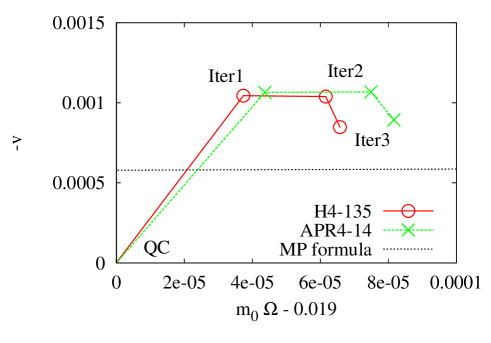
Figure 1 shows the values of $m_{0}\Omega$ and $v$ for all initial data computed in this study. As the eccentricity of Iter3 turns out to be smaller by an order of magnitude than that of QC (see Table 1), this figure indicates that the eccentricity reduction of quasicircular initial data with $m_{0}\Omega=0.019$ requires an increase of $\sim$ 0.3%–0.5% in the orbital angular velocity and the incorporation of an approaching velocity with $\sim$ 0.05%–0.1% of the speed of light. We further checked that Iter3 is closer to hypothetical Iter4 estimated from simulations of Iter3 than to Iter2 on this plot, and thus our eccentricity reduction procedure seems to converge toward a circularized state. A comparison between Iter3 values and a relation due to Mroué and Pfeiffer (MP), derived by fitting formulas for initial data of binary black holes mroue_pfeiffer2012 , suggests that the required orbital angular velocity and approaching velocity are larger and smaller, respectively, for initial data of binary neutron stars than those of binary black holes. To confirm this, we performed another simulation of the H4-135 family with $m_{0}\Omega$ and $v$ predicted by the MP formulas mroue_pfeiffer2012 with the same coordinate separation and found that the eccentricity is $\sim$ 0.0015. Note, however, that the meaning of coordinate separations is not rigorously the same due to different topology of spacetimes, whereas the gauge conditions are the same. In particular, this could lead to a large relative difference within the small range of $m_{0}\Omega$ and $v$ relevant here. Still, the eccentricity may be expressed as a Euclidean distance on a properly rescaled $(m_{0}\Omega,v)$ plane (see Eq. (22) of Ref. mroue_pfeiffer2012 ). This suggests that the fitting formulas do not produce low-eccentricity initial data with $e\lesssim$ 0.001 for binary neutron stars with $m_{0}\Omega\approx 0.019$, although they may be used to obtain first-trial initial data that are much better than quasicircular initial data.

Table 1 also shows the binding energy and total angular momentum of binary initial data. The Arnowitt–Deser–Misner mass $M_{0}$ and total angular momentum $J_{0}$ are computed by volume integrals gourgoulhon_gtmb2001 ; taniguchi_gourgoulhon2002 ; taniguchi_gourgoulhon2003 ; taniguchi_shibata2010 , and the binding energy is defined by $|M_{0}-m_{0}|$. It appears from the table that the energy and angular momentum of quasicircular orbits are too small to achieve low eccentricity. Order-of-magnitude estimates suggest that the dominant contributions to increases of $M_{0}$ and $J_{0}$ during the eccentricity reduction come from the increase of $m_{0}\Omega$, whereas the contribution of $v$ to the energy is negligible.

The global quantities can be compared with post-Newtonian formulas for binary neutron stars (see Appendix A). Here, we include point-particle contributions up to fourth post-Newtonian order blanchet2014 and finite-size contributions up to first post-Newtonian order to linear quadrupolar tidal deformation vines_flanagan2013 . The formulas predict $(|M_{0}-m_{0}|,J_{0})$ at $m_{0}\Omega=0.019$ to be $(0.0223M_{\odot},7.687M_{\odot}^{2})$ and $(0.0232M_{\odot},8.261M_{\odot}^{2})$ for H4-135 and APR4-14, respectively. Comparing these values with those shown in Table 1, it is found that the eccentricity reduction improves agreement of the angular momentum from $\sim$ 0.5% of QC to $\sim$ 0.1% of Iter3. Because the post-Newtonian approximation is expected to be an excellent approximation for the distant orbit computed here, this improvement suggests that low-eccentricity initial data are more accurate quasiequilibrium states than quasicircular ones.

IV.2 Orbital evolution and eccentricity

Before presenting the results, we briefly summarize the setup of numerical simulations. All the simulations in each model family are performed with a fixed size of the computational domain, $L$. Specifically, $L$ is $\approx$ 3400 km and 2600 km for the H4-135 and APR4-14 families, respectively. Computational domains of each simulation consist of five coarser domains, which are centered at the center of mass of the binary, and two sets of four finer domains, which follow the binary motion. The box size halves every refinement level, as does the grid separation. The grid separation at the finest domain $\Delta x_{\mathrm{min}}$ is $\approx$ 330 m and 250 m for H4-135 and APR4-14 families, respectively. These relatively coarse resolutions (see, e.g., Refs. hotokezaka_kkosst2013 ; hotokezaka_ks2013 ; hotokezaka_kkmsst2013 ) are not the product of compromise but are chosen to show that our eccentricity reduction works with low computational cost. To ensure that the eccentricity observed in simulations is independent of the grid resolution, we also perform simulations with $\Delta x_{\mathrm{min}}\approx$ 270 m (20% finer in terms of $1/\Delta x$) and 220 m (50% finer) for H4-135-QC and H4-135-Iter3.

Figure 2: The time derivative of coordinate orbital angular velocity, $\dot{\Omega}(t)$, of the H4-135 (left) and APR4-14 (right) families during the initial $\sim$ 3–4 orbits. In these plots, curves after taking the average over 100–200 time steps are shown. We exclude initial 2 ms from these plots, because data are not available for some models due to long averaging intervals.

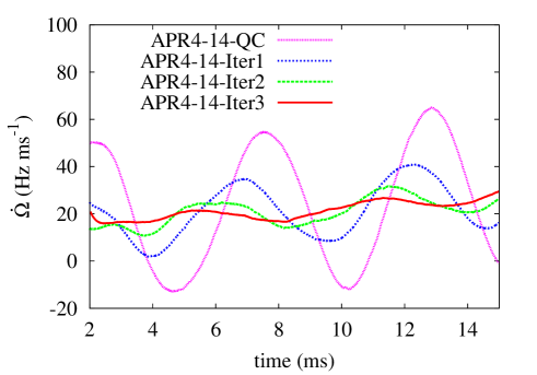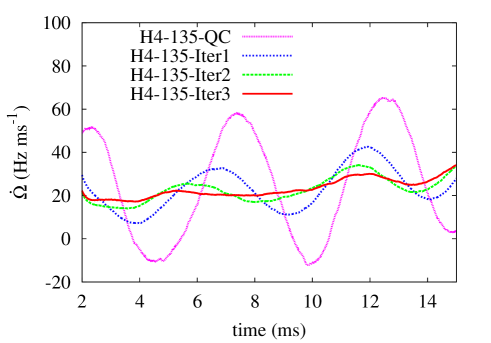
First of all, Fig. 2 shows $\dot{\Omega}(t)$ used to estimate corrections to initial data in the initial epoch of simulations. This figure shows that the amplitude of modulations in $\dot{\Omega}(t)$ decreases monotonically as the iterative eccentricity reduction proceeds. In particular, $\dot{\Omega}(t)$ of H4-135-QC and APR-14-QC become negative around their local minima, because the modulation amplitude is larger than the orbital average of $\dot{\Omega}(t)$. Negative values of $\dot{\Omega}(t)$ do not occur for all the other initial data, because our eccentricity reduction method succeeds in reducing the modulation in $\dot{\Omega}(t)$. It would be important, however, to check whether our method also diminishes eccentricity-driven modulations in other quantities that are not directly involved in the eccentricity reduction procedure.

Figure 3: The orbital evolution of the H4-135 (left) and APR4-14 (right) families during the initial $\sim$ 3–4 orbits. In these plots, Bezier curves are shown instead of raw data to focus on the eccentricity-driven modulation by discarding high-frequency oscillations associated with the finite grid separation (see Sec. III.2). We note that the Bezier smoothing is performed only for the presentation and is never adopted during the eccentricity reduction. The data averaged over 100–200 time steps behave very similarly to the Bezier curves, but we do not plot the former here, because some portion of initial abrupt decrease at $\lesssim$ 1 ms is masked by the averaging time interval.

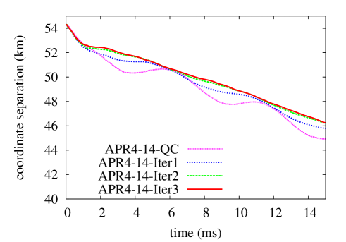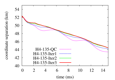
Figure 3 compares the orbital evolution of all the models in the initial epoch of simulations. Modulations with amplitude $\sim$ 0.5–1 km are observed in both H4-135-QC and APR4-14-QC, and the coordinate separations do not even decrease monotonically. These two models clearly exhibit the eccentricity inherent in quasicircular initial data. The modulations decay as the iterative eccentricity reduction proceeds, and it would not be easy to find oscillations of either H4-135-Iter3 or APR4-14-Iter3 in these plots by eye. This sharp decline in modulation is clear evidence of the efficacy of our eccentricity reduction method.

The eccentricity of initial data is evaluated by Eq. (37) and shown in Table 1. These values indicate that each iterative correction reduces the eccentricity by a factor of 2–3. As a result, three successive iterations reduce the eccentricity, $e\sim$ 0.01, of QC to $e\lesssim$ 0.001. Because this reduction factor is common to both the H4-135 and APR4-14 families, we believe it will not depend on the compactness of the neutron star. It could, however, vary with the mass ratio.

Figure 4: The orbital evolution of H4-135-QC during an initial orbit. The solid curve (zero shift) is the same as shown in Fig. 3, and derived giving initial data of gauge variables by $\alpha=W$, $\beta^{i}=0$, and $B^{i}=0$. The dashed oscillating curve (XCTS shift, where XCTS stands for extended conformal thin-sandwich) is derived giving $\alpha$ and $\beta^{i}$ obtained in the extended conformal thin-sandwich formulation, and $B^{i}=0$. In this figure, raw data are plotted to confirm that the initial trend is not an artifact of Bezier curves. This also indicates the uncertainty in determining the location of neutron stars by the maximum-density point, $x_{\mathrm{NS}}^{i}$.

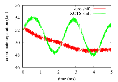
Aside from the eccentricity-driven modulation, an abrupt decrease of the coordinate orbital separation is found for all the models during the initial $\sim$ 1 ms, which is approximately one-fifth of the initial orbital period. Similar behavior is also observed in simulations of (spinning) binary black holes based on the moving puncture method tichy_marronetti2011 . We speculate that this decrease is due at least partly to the initial choice of the shift vector, $\beta^{i}=0$, while the relaxation from the spatial conformal flatness may also play a role. Figure 4 shows the orbital evolution during an initial orbit obtained with initial shift vectors $\beta^{i}=0$ and $\beta^{i}$ obtained in the extended conformal thin-sandwich formulation. The abrupt decrease is not observed with nonzero $\beta^{i}$, and instead the coordinate orbital separation increases due to another oscillation with approximately twice the frequency of the orbital one. Excitation of second harmonics in the coordinate orbital evolution due to $\beta^{i}$ obtained in the extended conformal thin-sandwich formulation has been found in simulations of binary black holes (see Appendix B of Ref. yamamoto_st2008 ). Because gauge-invariant quantities such as gravitational waves depend only weakly on the choice of initial shift vector, the harmonics should entirely be gauge artifacts. We also find that the coordinate evolution including the initial abrupt decrease is approximately unchanged when the harmonic gauge condition is adopted with the shift vector initialized by $\beta^{i}=0$. Taking the different orbital evolution after this initial transient among the models shown in Fig. 3 into account, we speculate that the abrupt decrease is caused by the relaxation of the shift vector from $\beta^{i}=0$, and not specific to the moving puncture gauge. If this abrupt decrease is eliminated by a sophisticated gauge choice, we would be able to use the numerical evolution data near $t=0$ for the eccentricity reduction, and this may improve the efficiency. By contrast, the eccentricity reduction becomes difficult due to the second harmonics if we adopt $\beta^{i}$ obtained in the extended conformal thin-sandwich formulation as initial values.

The periastron advance of binary neutron stars does not deviate significantly from that of binary black holes. The ratio of the radial frequency $\omega$ and orbital frequency $\Omega$ can be estimated in the fitting, and the initial value of $\Omega$ is typically larger than $\omega$ by $\sim$ 20%–25%. At the same time, the value of the angular velocity is estimated to be larger by $\sim$ 10% on average than its initial value during the fitting time interval, $[0.5P:3P]$, due to gravitational radiation reaction. Thus, the angular frequency is estimated to be larger by $\sim$ 30%–35% than the radial frequency. This fraction is consistent with results for binary black holes mroue_pkt2010 ; letiec_mbbpst2011 . Expected values for a test particle in the Schwarzschild spacetime are 32% and 39% for $m_{0}\Omega=0.019$ and 0.023 (value at $t\approx 3P$), respectively, and a third-order post-Newtonian calculation for an equal-mass binary gives 29% and 34% for $m_{0}\Omega=0.019$ and 0.023, respectively. Results of binary black hole simulations lie between these predictions, and binary neutron stars do not show significant deviations. More accurate estimation of a possible finite-size effect on the periastron advance will be an interesting topic for the future study.

Figure 5: The same as Fig. 3 but up to the merger. Oscillations after $\sim$ 30 ms show dynamics of remnant massive neutron stars with double-core structures hotokezaka_kkmsst2013 and thus are irrelevant to the orbital motion.

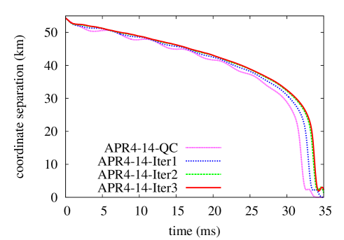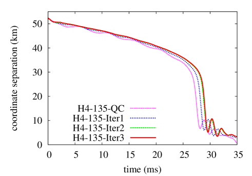
Figure 5 shows the orbital evolution up to the merger for all the models. It is observed that the eccentricity-driven modulation is very small during the entire inspiral phase for Iter3, whereas QC shows the modulation even right before the plunge. The eccentricity of quasicircular initial data should decrease as a result of gravitational radiation, but the rate is only $e(t)\propto[d(t)]^{19/12}$ at $e\ll 1$ in the quadrupole approximation. Hence, the expected decrease is only by a factor of $\sim$ 4 for the evolution (say) from $15m_{0}$ to $6m_{0}$, and quasicircular initial data with $\sim 0.01$ will never achieve a low-eccentricity inspiral with $e\lesssim 0.001$. Both analytic estimation and numerical results indicate that the eccentricity reduction has to be performed by improving initial data if we want to obtain the low-eccentricity, $e\lesssim 0.001$ inspiral with current computational resources.

The time to merger increases as the eccentricity decreases (see Fig. 5). While it is difficult to define the merger time in a physical manner from the orbital evolution, the time to merger seems to be longer by $\sim$ 2 ms for Iter3 than for QC. This cannot be explained by strong gravitational radiation from an eccentric binary, because the quadrupole formula predicts that the time to merger from a given semimajor axis is proportional to $1-(157/43)e^{2}$ at leading order of $e$ peters1964 : The eccentricity enters only through its squared value. The actual difference in the time to merger is, however, $\sim$ 5% between QC with $e\sim$ 0.01 and Iter3 with $\sim$ 0.001 and is thus too large. Instead, this difference is ascribed to the initial semimajor axis of the binary. Numerical results suggest that apastron distances are approximately the same irrespective of the eccentricity reduction, and the semimajor axis is shorter by $1-e$. Thus, the time to merger should be proportional to $1-4e$ at leading order of $e$. This approximately explains the difference of the time to merger shown in Fig. 5. This feature is consistent with findings in Ref. pfeiffer_bklls2007 that modulation-free parts of the orbital evolution and gravitational radiation are approximately independent of small eccentricity once appropriate time shifts are applied. This argument also suggests that quasicircular initial data computed assuming helical symmetry represent a binary configuration at the apastron. That is, the coordinate separation $d$ specified in the initial data computation is the apastron distance.

IV.3 Gravitational waves

The binary’s dynamical behavior is more reliably observed using gravitational waves, which are gauge invariant at least asymptotically. In SACRA, gravitational waves are extracted via the Weyl scalar $\Psi_{4}$ projected onto spin-weighted spherical harmonics at finite coordinate radii. We focus only on the $(\ell,m)=(2,2)$ mode in this study and denote its coefficient as $\Psi_{4,22}$. Although we extrapolate $\Psi_{4}$ to null infinity when we compute gravitational waves as transverse-traceless portions of the metric, we do not perform the extrapolation when we present $\Psi_{4}$ itself and instead show results obtained by extraction at $r_{\mathrm{ex}}\approx$ 300 km. We checked that $\Psi_{4}$ in the inspiral phase depends only weakly on the extraction radius once a time shift and amplitude scaling are performed according to the different extraction radii. We present gravitational-wave quantities as a function of an approximate retarded time defined using an approximate areal radius $D$ as

$$t_{\mathrm{ret}} \equiv t-D-2m_{0}\ln\left(\frac{D}{m_{0}}\right),$$ (41)

$$D \equiv r_{\mathrm{ex}}\left(1+\frac{m_{0}}{2r_{\mathrm{ex}}}\right)^{2}.$$ (42)

The total mass $m_{0}$ in these definitions should have been replaced by the Arnowitt–Deser–Misner mass, $M_{0}$, but we choose to avoid using $M_{0}$, because this depends on the stage of the eccentricity reduction as shown in Table 1. The difference between $m_{0}$ and $M_{0}$ does not introduce appreciable effects as far as we are concerned in this study.

Figure 6: The amplitude of $\Psi_{4,22}$ in the inspiral phase for the H4-135 (left) and APR4-14 (right) families. The amplitude is given by a dimensionless combination, $|\Psi_{4,22}|Dm_{0}$. The time is given by an approximate retarded time, and initial $\sim$ 0.1 ms suffers from junk radiation in initial data.

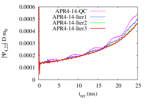Figure 6 shows the amplitude of $\Psi_{4,22}$ in the inspiral phase obtained from each model. Amplitudes of QC show substantial modulations in a similar manner to the orbital evolution. By contrast, those of IterX show only small modulations compared to QC, and again the modulations of Iter3 are not easily detected by eye except for small wiggles. The wiggles have higher frequency than the orbital frequency, and they are not induced by the eccentricity. Because gravitational-wave quantities are expected to be gauge invariant, this figure gives a firm evidence of the success of our eccentricity reduction. A comparison of Figs. 5 and 6 suggests that the eccentricity-driven modulations are approximately in phase for these two quantities, and thus discussions based on the coordinate orbital separation are not entirely gauge artifacts.

Figure 7: Gravitational waveforms for the H4-135 (left) and APR4-14 (right) families. The amplitude is given as that for an observer at 100 Mpc distance along the rotational axis of the binary. The plus mode gravitational waves of QC are drawn as a function of the approximate retarded time. Those of IterX are shifted in time so that the maximum amplitude occurs at the same time as QC and also shifted in phase so that polarization states approximately agree with that of QC.

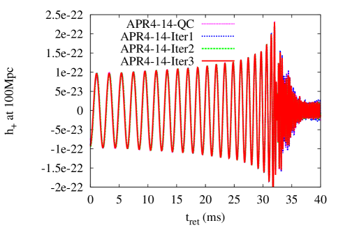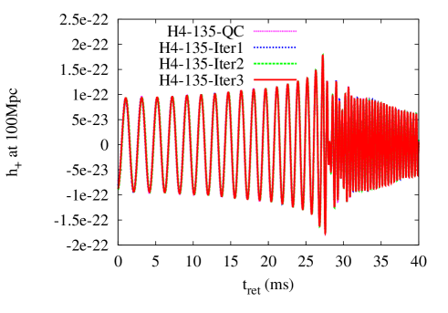
Gravitational waveforms are most important for the purpose of this study. To extract the waveforms, we extrapolate $\Psi_{4}$ to null infinity and perform a time integration as summarized in Appendix B. We plot plus-mode gravitational waves $h_{+}(t)$ in Fig. 7 after applying time and phase shifts to align the waveforms. The cross-mode $h_{\times}(t)$ shows the same behavior for the purpose of our discussion. Here, we again note that $h_{+}$ and $h_{\times}$ are real and (negative of) imaginary parts of the $(\ell,m)=(2,2)$ mode, respectively. This figure shows that the effect of an eccentricity $e\lesssim 0.01$ is not easily distinguished from the shifted gravitational waveforms, in either $\sim$ 10 orbits in the inspiral phase or a few tens of cycles in the postmerger phase. The former is already shown in the study of binary black holes pfeiffer_bklls2007 , and our result confirms this for binary neutron stars for the first time. This agreement will be made more quantitative when we compute the overlap or mismatch of the waveforms obtained by simulations, and we postpone such computations after hybridization with analytic models. The visual agreement of gravitational waveforms does not imply that quasicircular initial data are sufficient for the construction of theoretical templates, but properties of gravitational waves have to be investigated carefully as we do below.

Figure 8: Gravitational-wave amplitudes for the H4-135 (left) and APR4-14 (right) families in the inspiral phase. The vertical axis is the sum-squared amplitude measured by an observer at 100 Mpc distance along the rotational axis of the binary. The time axis is aligned so that the maximum amplitude occurs at the same time (outside these plots). QC and Iter1 suffer from junk radiation during the initial $\sim$ 1–2 ms, while junk radiation components of Iter2 and Iter3 are less apparent in the plots due to the time shifts.

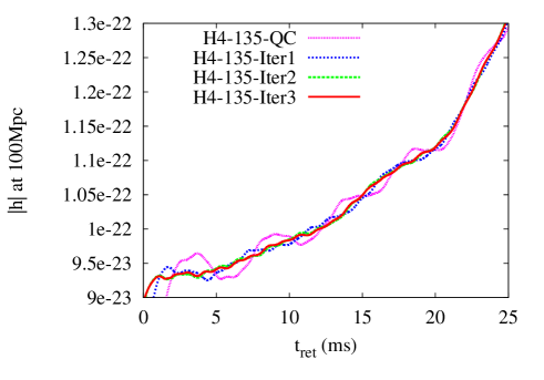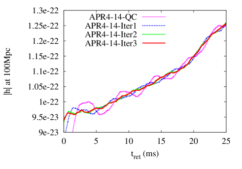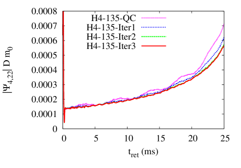
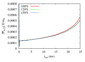
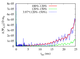
We move to more in-depth discussions by decomposing the gravitational waveforms into the amplitude and frequency. First, Fig. 8 shows the time evolution of the amplitude defined by

$$|h|(t)\equiv\sqrt{[h_{+}(t)]^{2}+[h_{\times}(t)]^{2}},$$ (43)

and the time shift is applied in the same manner as Fig. 7. Although the amplitude evolution of Iter3 is very smooth, those of QC with $e\sim$ 0.01 show the modulation with amplitude $\sim$ 3%–5% throughout the inspiral phase. This is roughly consistent with the expectation that the amplitude should vary by $(3/2)e$ at leading order of $e$ in the quadrupole approximation. In addition, these modulations are again in phase with the modulations observed in the orbital phase.

Figure 9: Time evolution of the eccentricity estimator, $e_{\mathrm{GW}}(t)$, defined from $\Omega_{\mathrm{GW}}(t)$ for the H4-135 (left) and APR4-14 (right) families in the inspiral phase. We truncate initial $\sim$ 5 ms for the fitting, because junk radiation pollutes $\Omega_{\mathrm{GW}}(t)$ in the initial orbit. After $\sim$ 25 ms, the evolution of the binary becomes plungelike, and the eccentricity may no longer be defined even approximately.

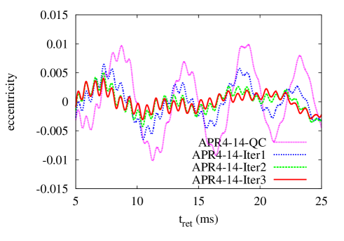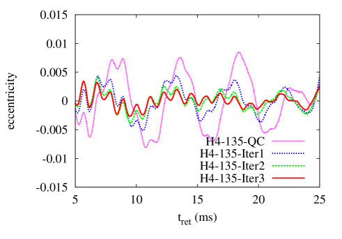
Next, we turn to the angular frequency of gravitational waves $\Omega_{\mathrm{GW}}(t)$ and show behavior of an eccentricity estimator instead of the angular frequency itself, which behaves very similarly to the amplitude shown in Fig. 8. The eccentricity estimator is defined using an underlying smooth evolution obtained by fitting, $\Omega_{\mathrm{GW,fit}}(t)$, as husa_hgsb2007

$$e_{\mathrm{GW}}(t)\equiv\frac{\Omega_{\mathrm{GW}}(t)-\Omega_{\mathrm{GW,fit}}(t)}{2\Omega_{\mathrm{GW,fit}}(t)}.$$ (44)

The fitting function is chosen to be polynomial in time,

$$\Omega_{\mathrm{GW,fit}}(t)=a_{0}+a_{1}t+a_{2}t^{2}+a_{3}t^{3}+a_{4}t^{4},$$ (45)

and features of $e_{\mathrm{GW}}(t)$ depend only weakly on the specific form of the fitting function. The fitting time interval is taken from $\sim$ 5 ms after the initial instant to $\sim$ 1 orbit before the merger, where the former is chosen to avoid strong unphysical effects of junk radiation.

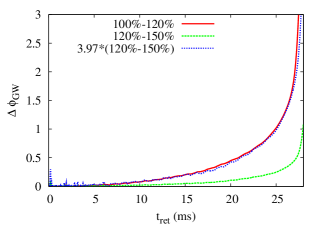
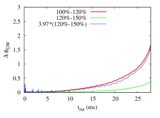
Figure 9 shows the time evolution of the eccentricity estimator, $e_{\mathrm{GW}}(t)$. The curves of QC exhibit oscillation components with the period $\sim$ 5 ms and amplitude $\sim$ 0.01, and this is ascribed to the orbital eccentricity in quasicircular initial data. This oscillation component with the period of $\sim$ 5 ms decays as the eccentricity reduction proceeds, and the curves of Iter3 show $\sim$ 5 ms oscillations with the amplitude of only $\sim$ 0.001. This behavior of the eccentricity estimator is consistent with the eccentricity evaluated in the fitting of orbital motion shown in Table 1, and thus both eccentricity estimation methods may be reliable.

When the orbital eccentricity is reduced to $\sim$ 0.001, another oscillation component with an amplitude $\sim$ 0.001 becomes prominent in the eccentricity estimator, $e_{\mathrm{GW}}$, with frequency several times higher than the orbital and radial frequencies. Indeed, this rapid component is not new to Iter3, and QC also exhibits this oscillatory behavior superposed on the eccentricity-driven modulation. This component does not converge away with increasing grid resolution as far as we tried. We also confirmed that this oscillation cannot be ascribed to the oscillation of neutron stars, since no oscillatory mode with the same frequency is found up to $\ell\leq 4$, including quadrupole oscillations, in our simulations. We speculate that this oscillation component is due to insufficient boundary conditions of SACRA, because the frequency of the oscillation changes when the location of the outer boundary is changed, although only slightly. We will confirm or exclude this speculation by implementing higher-order boundary conditions hilditch_btctb2013 in the near future. This will involve modifying the shape of the outer boundary. Another possibility is reflection of unphysical high-frequency radiation contained in initial data at adaptive-mesh-refinement boundaries zlochower_pl2012 , sizes of which are proportional to that of the outer boundary in SACRA. If this is the case, appropriately modified gauge conditions might reduce the rapid oscillation component etienne_bpks2014 .

Figure 10: Gravitational-wave spectra for the H4-135 (left) and APR4-14 (right) families. The vertical axis is the dimensionless amplitude, $f\tilde{h}(f)$, measured by an observer at 100 Mpc distance along the rotational axis of the binary. Abrupt decreases of the amplitude below $\sim$ 500 Hz are simply due to the fact that our simulations begin there. The spectra of H4-135 below and above $\sim$ 2000 Hz are contributions from the inspiral and remnant massive neutron star, respectively, and a similar separation holds for APR4-14 but at $\sim$ 2500 Hz. Spectral peaks associated with remnant massive neutron stars are systematically underestimated at high-frequency sides, because we truncate numerical data after $\sim$ 50 ms from the initial instant (or $\sim$ 20 ms after the merger) when remnants are still active. The peak frequency, where the maximum amplitude is achieved, does not vary by more than $\sim$ 10 Hz with the truncation.

We show the spectrum of gravitational waves in Fig. 10. Here, the effective spectral amplitude $\tilde{h}(f)$ is defined by

$$\tilde{h}(f)\equiv\sqrt{\frac{\left[\tilde{h}_{+}(f)\right]^{2}+\left[\tilde{h}_{\times}(f)\right]^{2}}{2}},$$ (46)

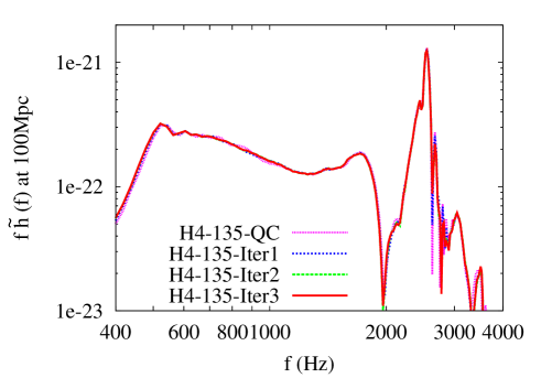
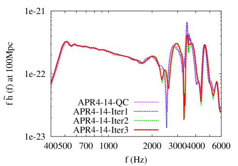
where $\tilde{h}_{+}(f)$ and $\tilde{h}_{\times}(f)$ are the Fourier transformation of the plus and cross modes, respectively. A remnant massive neutron star of neither H4-135-QC nor APR4-14-QC collapses to a black hole during simulations over $\sim$ 100 ms, and therefore we decided to stop H4-135-Iter3 and APR4-14-Iter3 only after $\sim$ 50 ms from the initial instant (or $\sim$ 20 ms after the merger). The same time interval of $\sim$ 50 ms is adopted among all the models for the computation of the spectra to avoid possible biases, even if longer data are available for some of the models. This truncation during the lifetime of remnant massive neutron stars results in an underestimation of the spectral peak at $\sim$ 2500 Hz and 3500 Hz for the H4-135 and APR4-14 families, respectively, associated with postmerger activities of the remnant massive neutron stars. This truncation mainly affects the high-frequency side of the spectral peak, and the frequency of the maximum amplitude does not vary by more than $\sim$ 10 Hz.

The effect of a small eccentricity, $e\lesssim 0.01$, on the spectra is weak both for inspiral and postmerger phases, in a similar manner to the waveforms shown in Fig. 7. This shows that previous studies of binary neutron stars focused on gravitational-wave spectra are not affected significantly by the orbital eccentricity if the simulation is sufficiently long. We find that the spectral amplitude is smoother for Iter3 in $\sim$ 600–1500 Hz than QC, and this is likely to reflect the reduced eccentricity. The difference is, however, relatively subtle and easily masked by different filtering techniques in Fourier transformation (see Appendix B). Thus, we only suggest that low-eccentricity initial data may yield smoother spectra than quasicircular ones. Figure 10 also suggests that characteristics of remnant massive neutron stars do not depend strongly on the eccentricity as again expected from the postmerger agreement in Fig. 7.

IV.4 Convergence

Figure 11: Convergence property of $\Psi_{4,22}$ for H4-135-QC with different grid resolutions. The high, middle, and low (baseline of this study) resolutions are denoted by 150%, 120%, and 100%, respectively. The left, middle, and right panels show the amplitude evolution, difference of amplitude evolution, and difference of phase evolution, respectively. We do not show the phase evolution itself, because differences among different grid resolutions are barely distinguished from the direct comparison. We also include a rescaled difference between high and middle resolutions using a scaling factor 3.97 obtained assuming a hypothetical eighth-order convergence for difference plots.

Figure 12: The same as Fig. 11, but for H4-135-Iter3. The time intervals are taken to be the same as those of Fig. 11 in all the plots. Because the merger time is later for H4-135-Iter3 than for H4-135-QC, the amplitude and phase differences at the end of the plots are smaller accordingly.

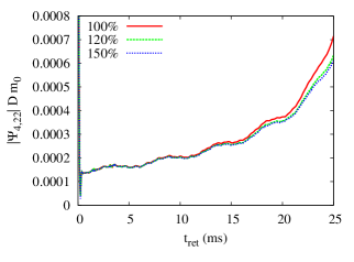
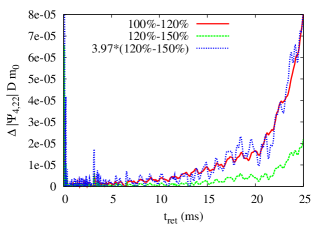
We discuss convergence issues to show that the presence and/or absence of eccentricity-driven modulations found in various quantities are inherent in initial data rather than associated with the finite grid resolution. Figure 11 compares the evolution of quantities associated with $\Psi_{4,22}$ for H4-135-QC among high, middle, and low resolutions, where the low resolution has always been adopted to derive all the results presented so far. The left panel shows the amplitude evolution and indicates that the modulations with a $\sim$ 5 ms period are in phase among all the grid resolutions. Furthermore, the differences of the amplitude plotted in the middle panel show no modulation with this period. These facts imply that the eccentricity is a genuine property of initial data. Figure 12 shows the same quantities as Fig. 11 but for H4-135-Iter3, and no appreciable eccentricity-driven modulation is observed in either the amplitude itself or its difference. This fact implies that the low eccentricity of H4-135-Iter3 is not an artifact of a particular grid setting and is again a genuine property of initial data.

The middle panels of Figs. 11 and 12 also suggest that the result of new SACRA with the Z4c formulation converges more rapidly than that of the previous version yamamoto_st2008 . Although our evolution scheme is fourth order at best in both time and space, the overall behavior of the amplitude evolution among different resolutions implies that our results are scaled with eighth-order convergence even right before the merger (compare with Fig. 7). Specifically, we assume that a quantity $Q$ depends on the grid separation $\Delta x$ as

$$Q(\Delta x)=Q_{0}+E(\Delta x)^{p},$$ (47)

where $Q_{0}\equiv Q(0)$ is the value at the continuum limit, $E$ is a constant, and $p$ is the convergence order. We readily derive

$$\frac{Q(\Delta x)-Q(\Delta x/1.2)}{Q(\Delta x/1.2)-Q(\Delta x/1.5)}=\frac{1-1/(1.2)^{p}}{1/(1.2)^{p}-1/(1.5)^{p}}.$$ (48)

Our numerical results suggest that the left-hand side is approximately equal to 4, and this is explained if $p\approx 8$. We never expect that our new code converges with the eighth order, which might be achieved when lower-order truncation errors happen to be very small. We guess rather that the range of grid resolutions spanned in this study, 150%, is not sufficient to clarify the convergence property in a nearly convergent regime. A more systematic investigation spanning a wide range of grid resolutions is evidently required. It should be cautioned that assessment of convergence properties in numerical relativity is a highly nontrivial task, especially when a sophisticated adaptive-mesh-refinement algorithm is adopted zlochower_pl2012 . As SACRA has been verified in many places with the BSSN formulation (see, e.g., Ref. read_bcfgkmrst2013 ), our results convince us that the modulation is not an artifact of finite grid resolutions.

The right panels of Figs. 11 and 12 compare gravitational-wave phase evolution among different grid resolutions. Again, we see no modulation with the $\sim$ 5 ms period in the phase differences, and thus the eccentricity is shown to be inherent in initial data. An apparent eighth-order convergence is also found in the phase evolution in a manner consistent with the amplitude evolution. A small phase difference of $\sim$ 1 radian between middle and high resolutions at $t_{\mathrm{ret}}=28$ ms may be more important for practical purposes, where this approximately corresponds to $m_{0}\Omega_{\mathrm{GW}}=0.1$ for H4-135-QC. The small difference should be contrasted with previous results obtained in the BSSN formulation, with which the number of orbits can differ by a factor of order unity with a similar grid resolution hotokezaka_ks2013 . While a sophisticated extrapolation method such as the one developed in Ref. hotokezaka_ks2013 will be still useful to compute physical waveforms, slight improvement of the grid resolution would give us a phase error smaller than 0.1 radian, accurate enough for the next generation of interferometric detectors.

V Summary and discussion

We developed a method to obtain low-eccentricity initial data of binary neutron stars for numerical relativity. In the beginning, we computed standard quasicircular initial data assuming helical symmetry with the angular velocity determined by force balance at the center of neutron stars gourgoulhon_gtmb2001 ; taniguchi_gourgoulhon2002 ; taniguchi_gourgoulhon2003 ; taniguchi_shibata2010 , and evolved them for $\sim$ 3 orbits. We fit the time derivative of the coordinate orbital angular velocity to an analytic function and estimated appropriate corrections to the orbital angular velocity and approaching velocity for the eccentricity reduction. We then modified the initial data by adjusting the orbital angular velocity and approaching velocity. This modification affected the solution primarily through the hydrostatic equilibrium equations for binary neutron stars and should be contrasted with the case of binary black holes pfeiffer_bklls2007 ; husa_hgsb2007 . We repeated these procedures (initial data computation, time evolution, and analysis of the orbit) until the eccentricity was reduced to a desired value.

We demonstrated the ability of our eccentricity reduction by simulating two families of equal-mass binary neutron stars. The eccentricity was decreased from $\sim$ 0.01 to $\lesssim$ 0.001 by three successive iterations beginning with quasicircular initial data. We found that low-eccentricity initial data exhibit smaller modulations in evolution of the orbital separation, gravitational-wave amplitude, and gravitational-wave frequency than quasicircular initial data. Smooth evolution of gravitational-wave quantities associated with low-eccentricity initial data will help comparisons with analytic models and hybridization to construct theoretical templates. We also found that the accuracy of gravitational waves derived by low-eccentricity initial data is limited by high-frequency oscillations, which might be ascribed to insufficient outer boundary conditions of SACRA.

Aside from gravitational waves investigated in this study, the eccentricity could affect properties of remnant massive neutron stars and mass ejection from the system, and hence electromagnetic signals. Indeed, simulations performed in this study suggest that the ejecta mass, which is $3\times 10^{-4}M_{\odot}$ for H4-135-QC and $0.02M_{\odot}$ for APR4-14-QC at 10 ms after the merger, seems to vary by $O(10\%)$ between quasicircular and low-eccentricity initial data. This variation is not always systematic with respect to the eccentricity, possibly because the velocity at the contact of binary neutron stars can fluctuate within the eccentricity-driven modulation in each particular simulation. We do not present results for them in detail here, because quantitative conclusions require systematic investigations with convergence analysis. Remnant massive neutron stars and mass ejection will be relevant to short-hard gamma-ray bursts (see Refs. nakar2007 ; berger2014 and references therein for reviews) and other electromagnetic counterparts li_paczynski1998 ; nakar_piran2011 , and thus the eccentricity reduction may also be important to quantitatively clarify electromagnetic signals from binary neutron star mergers.

Appendix A Post-Newtonian formula

The energy and angular momentum of a binary of nonspinning masses $m_{1}$ and $m_{2}$ with the angular velocity $\Omega$ are currently known up to fourth post-Newtonian order for point-particle contributions blanchet2014 . Here, the total mass is defined by $m_{0}\equiv m_{1}+m_{2}$, and the symmetric mass ratio is defined by $\nu\equiv m_{1}m_{2}/m_{0}^{2}$. A post-Newtonian parameter is defined by

$$x\equiv\left(\frac{Gm_{0}\Omega}{c^{3}}\right)^{2/3},$$ (49)

where $G$ and $c$ are inserted for clarity in this Appendix. The orbital binding energy is given by

$$\frac{E}{m_{0}c^{2}}=-\frac{\nu x}{2}\biggl{\{} 1+\left(-\frac{3}{4}-\frac{\nu}{12}\right)x+\left(-\frac{27}{8}+\frac{19}{8}\nu-\frac{\nu^{2}}{24}\right)x^{2}$$

$$+ \left(-\frac{675}{64}+\left[\frac{34445}{576}-\frac{205}{96}\pi^{2}\right]\nu-\frac{155}{96}\nu^{2}-\frac{35}{5184}\nu^{3}\right)x^{3}$$

$$+ \biggl{(}-\frac{3969}{128}+\left[-\frac{123671}{5760}+\frac{9037}{1536}\pi^{2}+\frac{1792}{15}\ln 2+\frac{896}{15}\gamma_{\mathrm{E}}\right]\nu$$

$$+ \left[-\frac{498449}{3456}+\frac{3157}{576}\pi^{2}\right]\nu^{2}+\frac{301}{1728}\nu^{3}+\frac{77}{31104}\nu^{4}+\frac{448}{15}\nu\ln x\biggr{)}x^{4}\biggr{\}},$$ (50)

where $\gamma_{\mathrm{E}}$ is Euler’s constant. The orbital angular momentum is given by

$$\frac{J}{Gm_{0}^{2}/c}=\frac{\nu}{x^{1/2}}\biggl{\{} 1+\left(\frac{3}{2}+\frac{\nu}{6}\right)x+\left(\frac{27}{8}-\frac{19}{8}\nu+\frac{\nu^{2}}{24}\right)x^{2}$$

$$+ \left(\frac{135}{16}+\left[-\frac{6889}{144}+\frac{41}{24}\pi^{2}\right]\nu+\frac{31}{24}\nu^{2}+\frac{7}{1296}\nu^{3}\right)x^{3}$$

$$+ \biggl{(}\frac{2835}{128}+\left[\frac{98869}{5760}-\frac{6455}{1536}\pi^{2}-\frac{256}{3}\ln 2-\frac{128}{3}\gamma_{\mathrm{E}}\right]\nu$$

$$+ \left[\frac{356035}{3456}-\frac{2255}{576}\pi^{2}\right]\nu^{2}-\frac{215}{1728}\nu^{3}-\frac{55}{31104}\nu^{4}-\frac{64}{3}\nu\ln x\biggr{)}x^{4}\biggr{\}}.$$ (51)

The latter is derived from the former using a so-called thermodynamic relation,

$$\frac{\partial E}{\partial\Omega}=\Omega\frac{\partial J}{\partial\Omega},$$ (52)

or equivalently

$$\frac{\partial[E/(m_{0}c^{2})]}{\partial x}=x^{3/2}\frac{\partial[J/(Gm_{0}^{2}/c)]}{\partial x}.$$ (53)

Finite-size contributions are computed up to first post-Newtonian order to linear quadrupolar tidal deformation vines_flanagan2013 . We parametrize the finite-size effect of a neutron star with the gravitational mass $m$ and radius $R$ by a dimensionless quadrupolar tidal deformability defined by lackey_ksbf2012 ; lackey_ksbf2014

$$\Lambda=G\lambda\left(\frac{c^{2}}{Gm}\right)^{5}=\frac{2}{3}k\left(\frac{c^{2}R}{Gm}\right)^{5},$$ (54)

where $\lambda$ and $k$ are the quadrupolar tidal deformability and Love number, respectively. Specific values of $\Lambda$ are 1111 for a $1.35M_{\odot}$ neutron star with the H4 equation of state and 256 for a $1.4M_{\odot}$ neutron star with the APR4 equation of state. Hereafter, the dimensionless deformability of $m_{1}$ and $m_{2}$ are denoted by $\Lambda_{1}$ and $\Lambda_{2}$, respectively. We further define $q_{1}\equiv m_{1}/m_{0}$ and $q_{2}\equiv m_{2}/m_{0}$. The contribution to the orbital binding energy is

$$\frac{E_{\mathrm{tidal}}}{m_{0}c^{2}}=\frac{\nu x}{2}\biggl{\{}9\biggl{(} q_{1}^{4}q_{2}\Lambda_{1}+q_{1}q_{2}^{4}\Lambda_{2}\biggr{)}x^{5}$$

$$+\frac{11}{2}\biggl{[} (3+2q_{1}+3q_{1}^{2})q_{1}^{4}q_{2}\Lambda_{1}$$

$$+ (3+2q_{2}+3q_{2}^{2})q_{1}q_{2}^{4}\Lambda_{2}\biggr{]}x^{6}\biggr{\}},$$ (55)

and that to the orbital angular momentum is

$$\frac{J_{\mathrm{tidal}}}{Gm_{0}^{2}/c}=\frac{\nu}{x^{1/2}}\biggl{\{}6\biggl{(} q_{1}^{4}q_{2}\Lambda_{1}+q_{1}q_{2}^{4}\Lambda_{2}\biggr{)}x^{5}$$

$$+\frac{7}{2}\biggl{[} (3+2q_{1}+3q_{1}^{2})q_{1}^{4}q_{2}\Lambda_{1}$$

$$+ (3+2q_{2}+3q_{2}^{2})q_{1}q_{2}^{4}\Lambda_{2}\biggr{]}x^{6}\biggr{\}},$$ (56)

where the thermodynamic relation is used again. These contributions are simply added to the point-particle contributions described above. For $Gm_{0}\Omega/c^{3}=0.019$ considered in this study, point-particle terms up to second post-Newtonian order dominate the energy and angular momentum, while the sum of higher-order terms and finite-size corrections contribute only by $\sim$ 0.1%–0.2% even for a relatively stiff H4 equation of state.

Appendix B Computation of gravitational waves

In this Appendix, we summarize our derivation of gravitational waveforms $h=h_{+}-\mathrm{i}h_{\times}$ from $\Psi_{4}$ obtained by numerical simulations. We first extrapolate $\Psi_{4}$ extracted at a finite coordinate radius, $r_{\mathrm{ex}}$, to null infinity following Ref. lousto_nzc2010 . Using the areal radius defined by Eq. (42), we compute

$$\left.D\Psi_{4,\ell m}(t)\right|_{D\to\infty}=\left(1-\frac{2m_{0}}{D}\right)$$

$$\times\left[D\Psi_{4,\ell m}(t)-\frac{(\ell-1)(\ell+2)}{2}\int\Psi_{4,\ell m}(t^{\prime})dt^{\prime}\right],$$ (57)

where $\Psi_{4,\ell m}$ is the $(\ell,m)$-mode coefficient of $\Psi_{4}$ projected onto spin-weighted spherical harmonics. The prefactor $1-2m_{0}/D$ approximately corrects a difference between the tetrad used in SACRA yamamoto_st2008 and the Kinnersly tetrad, where the latter has to be chosen to derive this extrapolation formula. Next, gravitational waveforms are computed by integrating this extrapolated $\Psi_{4}$ (or $D\Psi_{4}$) twice as

$$h_{\ell m}(t)=\int\left(\int\Psi_{4,\ell m}(t^{\prime\prime})dt^{\prime\prime}\right)dt^{\prime}.$$ (58)

The angular frequency of gravitational waves, $\Omega_{\mathrm{GW}}(t)$, is estimated by

$$\Omega_{\mathrm{GW},\ell m}(t)\equiv\frac{|\int\Psi_{4,\ell m}(t^{\prime})dt^{\prime}|}{|\int\left(\int\Psi_{4,\ell m}(t^{\prime\prime})dt^{\prime\prime}\right)dt^{\prime}|}.$$ (59)

In the body text, we suppress the subscript $\ell m$ except for $\Psi_{4,22}$, because we focus only on the $(2,2)$ mode.

All the time integrations are performed by fixed-frequency integration reisswig_pollney2011 . The time-domain data are transformed to frequency-domain data by

$$\tilde{\Psi}_{4,\ell m}(f)=\int w(t)\Psi_{4,\ell m}(t)e^{-2\pi\mathrm{i}ft}dt,$$ (60)

where we apply a tapered-cosine filter of the form

$$w(t)=\begin{cases}\{1-\cos[\pi(t-t_{i})/\Delta t]\}/2&(t_{i}\leq t<t_{i+})\\ 1&(t_{i+}\leq t<t_{f-})\\ \{1-\cos[\pi(t_{f}-t)/\Delta t]\}/2&(t_{f-}\leq t<t_{f})\end{cases}.$$ (61)

Here, $t_{i}$ and $t_{f}$ are the initial and final times of the data, respectively, and $t_{i+}\equiv t_{i}+\Delta t$ and $t_{f-}\equiv t_{f}-\Delta t$ are determined by a width of the tapering region $\Delta t$. We choose $\Delta t\approx$ 1 ms for the computation of waveforms. Gravitational waveforms are computed as

$$h_{\ell m}(t)=-\int\frac{\tilde{\Psi}_{4,\ell m}(f)}{(2\pi\max[f,f_{0}])^{2}}e^{2\pi\mathrm{i}ft}df,$$ (62)

replacing the time integration with multiplication by $-\mathrm{i}/(2\pi f)$. Here, a fixed frequency $f_{0}$ is introduced to suppress unphysical drifts associated with spurious contributions from low-frequency components, and we choose it to be $f_{0}=0.8m(\Omega/2\pi)$ so that physical information of gravitational waves is not affected. This integration method is also used in evaluating the right-hand side of Eq. (57).

Gravitational-wave spectra are computed by Eq. (60) and double multiplication of $-\mathrm{i}/(2\pi f)$. For this purpose, we apply the tapered-cosine filter, Eq. (61), with $\Delta t\approx$ 5 ms to remove unphysical noises (in the frequency domain) associated with junk radiation and finite data length.

References

- (1) J. A. Faber and F. A. Rasio, Living Rev. Relativity 15, 8 (2012)
- (2) P. C. Peters, Phys. Rev. 136, B1224 (1964)
- (3) C. S. Kochanek, Astrophys. J. 398, 234 (1992)
- (4) L. Bildsten and C. Cutler, Astrophys. J. 400, 175 (1992)
- (5) D. R. Lorimer, Living Rev. Relativity 11, 8 (2008)
- (6) K. Hotokezaka, K. Kiuchi, K. Kyutoku, T. Muranushi, Y.-I. Sekiguchi, M. Shibata, and K. Taniguchi, Phys. Rev. D 88, 044026 (2013)
- (7) K. Hotokezaka, K. Kyutoku, Y.-I. Sekiguchi, and M. Shibata (unpublished)
- (8) K. Hotokezaka, K. Kiuchi, K. Kyutoku, H. Okawa, Y.-I. Sekiguchi, M. Shibata, and K. Taniguchi, Phys. Rev. D 87, 024001 (2013)
- (9) K. Hotokezaka, K. Kyutoku, and M. Shibata, Phys. Rev. D 87, 044001 (2013)
- (10) J. S. Read, L. Baiotti, J. D. E. Creighton, J. L. Friedman, B. Giacomazzo, K. Kyutoku, C. Markakis, L. Rezzolla, M. Shibata, and K. Taniguchi, Phys. Rev. D 88, 044042 (2013)
- (11) E. Gourgoulhon, P. Grandclément, K. Taniguchi, J.-A. Marck, and S. Bonazzola, Phys. Rev. D 63, 064029 (2001)
- (12) K. Taniguchi and E. Gourgoulhon, Phys. Rev. D 66, 104019 (2002)
- (13) K. Taniguchi and E. Gourgoulhon, Phys. Rev. D 68, 124025 (2003)
- (14) K. Taniguchi and M. Shibata, Astrophys. J. Suppl. 188, 187 (2010)
- (15) S. Bonazzola, E. Gourgoulhon, and J.-A. Marck, Phys. Rev. D 56, 7740 (1997)
- (16) H. Asada, Phys. Rev. D 57, 7292 (1998)
- (17) M. Shibata, Phys. Rev. D 58, 024012 (1998)
- (18) S. A. Teukolsky, Astrophys. J. 504, 442 (1998)
- (19) K. Kiuchi, Y. Sekiguchi, M. Shibata, and K. Taniguchi, Phys. Rev. D 80, 064037 (2009)
- (20) P. Tsatsin and P. Marronetti, Phys. Rev. D 88, 064060 (2013)
- (21) H. P. Pfeiffer, D. A. Brown, L. E. Kidder, L. Lindblom, G. Lovelace, and M. A. Scheel, Classical Quantum Gravity 24, S59 (2007)
- (22) A. Buonanno, G. B. Cook, and F. Pretorius, Phys. Rev. D 75, 124018 (2007)
- (23) M. Boyle, D. A. Brown, L. E. Kidder, A. H. Mroué, H. P. Pfeiffer, M. A. Scheel, G. B. Cook, and S. A. Teukolsky, Phys. Rev. D 76, 124038 (2007)
- (24) M. Hannam, S. Husa, J. A. González, U. Sperhake, and B. Brügmann, Phys. Rev. D 77, 044020 (2008)
- (25) L. Baiotti, T. Damour, B. Giacomazzo, A. Nagar, and L. Rezzolla, Phys. Rev. D 84, 024017 (2011)
- (26) S. Bernuzzi, A. Nagar, M. Thierfelder, and B. Brügmann, Phys. Rev. D 86, 044030 (2012)
- (27) B. D. Lackey, K. Kyutoku, M. Shibata, P. R. Brady, and J. L. Friedman, Phys. Rev. D 85, 044061 (2012)
- (28) F. Pannarale, E. Berti, K. Kyutoku, and M. Shibata, Phys. Rev. D 88, 084011 (2013)
- (29) F. Foucart, M. B. Deaton, M. D. Duez, L. E. Kidder, I. MacDonald, C. D. Ott, H. P. Pfeiffer, M. A. Scheel, B. Szilágyi, and S. A. Teukolsky, Phys. Rev. D 87, 084006 (2013)
- (30) B. D. Lackey, K. Kyutoku, M. Shibata, P. R. Brady, and J. L. Friedman, Phys. Rev. D 89, 043009 (2014)
- (31) M. Favata, Phys. Rev. Lett. 112, 101101 (2014)
- (32) K. Yagi and N. Yunes, Phys. Rev. D 89, 021303 (2014)
- (33) L. Wade, J. D. E. Creighton, E. Ochsner, B. D. Lackey, B. F. Farr, T. B. Littenberg, and V. Raymond, Phys. Rev. D 89, 103012 (2014)
- (34) R. Haas et al. (private communication)
- (35) I. Hinder et al., Classical Quantum Gravity 31, 025012 (2014)
- (36) M. Shibata and T. Nakamura, Phys. Rev. D 52, 5428 (1995)
- (37) T. W. Baumgarte and S. L. Shapiro, Phys. Rev. D 59, 024007 (1998)
- (38) S. Bernuzzi and D. Hilditch, Phys. Rev. D 81, 084003 (2010)
- (39) J. W. York, Phys. Rev. Lett. 82, 1350 (1999)
- (40) H. P. Pfeiffer and J. W. York, Phys. Rev. D 67, 044022 (2003)
- (41) LORENE website, http://www.lorene.obspm.fr/.
- (42) S. Bonazzola, E. Gourgoulhon, and J.-A. Marck, Phys. Rev. D 58, 104020 (1998)
- (43) T. Yamamoto, M. Shibata, and K. Taniguchi, Phys. Rev. D 78, 064054 (2008)
- (44) D. Hilditch, S. Bernuzzi, M. Thierfelder, Z. Cao, W. Tichy, and B. Brügmann, Phys. Rev. D 88, 084057 (2013)
- (45) M. Pürrer, S. Husa, and M. Hannam, Phys. Rev. D 85, 124051 (2012)
- (46) K. Kyutoku, M. Shibata, and K. Taniguchi, Phys. Rev. D 79, 124018 (2009)
- (47) A. Buonanno, L. E. Kidder, A. H. Mroué, H. P. Pfeiffer, and A. Taracchini, Phys. Rev. D 83, 104034 (2011)
- (48) A. H. Mroué, H. P. Pfeiffer, L. E. Kidder, and S. A. Teukolsky, Phys. Rev. D 82, 124016 (2010)
- (49) B. D. Lackey, M. Nayyar, and B. J. Owen, Phys. Rev. D 73, 024021 (2006)
- (50) A. Akmal, V. R. Pandharipande, and D. G. Ravenhall, Phys. Rev. C 58, 1804 (1998)
- (51) J. S. Read, B. D. Lackey, B. J. Owen, and J. L. Friedman, Phys. Rev. D 79, 124032 (2009)
- (52) A. H. Mroué and H. P. Pfeiffer, arXiv:1210.2958
- (53) L. Blanchet, Living Rev. Relativity 17, 2 (2014)
- (54) J. E. Vines and É. É. Flanagan, Phys. Rev. D 88, 024046 (2013)
- (55) W. Tichy and P. Marronetti, Phys. Rev. D 83, 024012 (2011)
- (56) A. Le Tiec, A. H. Mroué, L. Barack, A. Buonanno, H. P. Pfeiffer, N. Sago, and A. Taracchini, Phys. Rev. Lett. 107, 141101 (2011)
- (57) F. Foucart, L. Buchman, M. D. Duez, M. Grudich, L. E. Kidder, I. MacDonald, A. Mroue, H. P. Pfeiffer, M. A. Scheel, and B. Szilagyi, Phys. Rev. D 88, 064017 (2013)
- (58) S. Husa, M. Hannam, J. A. González, U. Sperhake, and B. Brügmann, Phys. Rev. D 77, 044037 (2008)
- (59) Y. Zlochower, M. Ponce, and C. O. Lousto, Phys. Rev. D 86, 104056 (2012)
- (60) Z. B. Etienne, J. G. Baker, V. Paschalidis, B. J. Kelly, and S. L. Shapiro, arXiv:1404.6523
- (61) E. Nakar, Phys. Rep. 442, 166 (2007)
- (62) E. Berger, Annu. Rev. Astron. Astrophys. 52, 43 (2014)
- (63) L.-X. Li and B. Paczyński, Astrophys. J. 507, L59 (1998)
- (64) E. Nakar and T. Piran, Nature (London) 478, 82 (2011)
- (65) C. O. Lousto, H. Nakano, Y. Zlochower, and M. Campanelli, Phys. Rev. D 82, 104057 (2010)
- (66) C. Reisswig and D. Pollney, Classical Quantum Gravity 28, 195015 (2011)