Transition from inspiral to plunge in precessing binaries of spinning black holes

Abstract

We investigate the non-adiabatic dynamics of spinning black hole binaries by using an analytical Hamiltonian completed with a radiation-reaction force, containing spin couplings, which matches the known rates of energy and angular momentum losses on quasi-circular orbits. We consider both a straightforward post-Newtonian-expanded Hamiltonian (including spin-dependent terms), and a version of the resummed post-Newtonian Hamiltonian defined by the Effective One-Body approach. We focus on the influence of spin terms onto the dynamics and waveforms. We evaluate the energy and angular momentum released during the final stage of inspiral and plunge. For an equal-mass binary the energy released between 40 Hz and the frequency beyond which our analytical treatment becomes unreliable is found to be, when using the more reliable Effective One-Body dynamics: $0.6\%M$ for anti-aligned maximally spinning black holes, $5\%M$ for aligned maximally spinning black hole, and $1.8\%M$ for non-spinning configurations. In confirmation of previous results, we find that, for all binaries considered, the dimensionless rotation parameter $J/E^{2}$ is always smaller than unity at the end of the inspiral, so that a Kerr black hole can form right after the inspiral phase. By matching a quasi-normal mode ringdown to the last reliable stages of the plunge, we construct complete waveforms approximately describing the gravitational wave signal emitted by the entire process of coalescence of precessing binaries of spinning black holes.

I Introduction

An international network of kilometer-scale laser-interferometric gravitational-wave detectors, consisting of the Laser-Interferometer Gravitational-wave Observatory (LIGO) LIGO , of VIRGO VIRGO , of GEO 600 GEO and of TAMA 300 TAMA , has by now begun the science operations. TAMA 300 reached its full design sensitivity in 2001, VIRGO is in its commissioning phase and plans to start the first scientific runs by the end of 2005, while LIGO has already completed three science runs (two of them in coincidence with GEO 600) with increasing sensitivity and duty cycle. LIGO and GEO 600 are expected to reach their full design sensitivity in 2005.

Binary black holes are among the most promising sources for these detectors. Among black hole binaries, it was emphasized in TD that there is a bias towards first detecting mostly aligned spinning binaries with high masses, whose last stable spherical orbits are drawn, by spin effects, to larger binding energies, yet due to their high masses these energies are still emitted through gravitational waves in the sensitive band of the detectors. Studying in detail the waveforms emitted during the last stages of dynamical evolution of such heavy spinning black hole binaries, with explicit consideration of the crucial transition between adiabatic inspiral and plunge, is a demanding theoretical challenge. The aim of the present paper is to provide a first attack on this problem by using some of the best analytical tools currently available to describe the transition from adiabatic inspiral to plunge, and notably the Effective One Body (EOB) approach BD1 ; BD2 .

So far, most theoretical and data-analysis studies on precessing binaries of spinning black holes assumed adiabatic evolution. Thus they were restricted to considering only the inspiral phase ACST94 ; K ; apostolatos0 ; apostolatos1 ; apostolatos2 ; GKV ; GK ; bcv2 ; pbcv1 ; bcpv1 ; Gpc . Actually, even for non-spinning binary configurations, most theoretical studies confined themselves to considering the adiabatic inspiral phase, though a lot of effort was spent to improve the accuracy of the phasing during the last stages of the inspiral, see e.g. DIS98 ; DIS00 .

For heavy black hole binaries, most of the signal-to-noise ratio in the ground detectors will come from the very last stages of the inspiral, and from the non-adiabatic transition between inspiral and plunge. It is therefore essential to be able to describe, with acceptable accuracy, this non-adiabatic evolution. In Refs. BD1 ; BD2 a new way of describing the dynamics of binary systems was introduced: the Effective One-Body (EOB) approach. The EOB approach uses both a specific resummation of the post-Newtonian Hamiltonian, and a resummed version of radiation reaction. This was shown to lead to a rather robust formalism, which is likely to provide a reliable description of non-adiabatic effects, of the transition between inspiral and plunge, and of the beginning of the plunge. It was also used in BD2 to model the full merger phase of non-spinning binaries, by matching the natural end of the EOB plunge with the ring-down phase. The EOB approach was used in Refs. BD2 ; DJS to derive non-adiabatic template waveforms emitted by non-spinning black hole binaries. It was shown in DIS01 that these new EOB templates led to significantly enhanced signal to noise ratios in current detectors (mainly because of the inclusion of the plunge signal). The EOB Hamiltonian was extended to the case of spinning black holes in TD . The analytical predictions made by the EOB method (including spin) were found to agree remarkably well DGG with the numerical results obtained by means of the helical Killing vector approach GGB for circular orbits of corotating black holes. Several other studies showed that the EOB method provides phasing models which are more reliable and robust than other (adiabatic or non-adiabatic) models bcv1 ; DIS03 .

The main purpose of this paper is to extend the use of the EOB approach to the case of precessing binaries of spinning black holes, both by including spin-dependent terms in radiation-reaction effects, and by studying the waveforms generated beyond the adiabatic approximation, i.e. taking into account the transition between inspiral and plunge, and the plunge itself. Let us emphasize again that the EOB approach has the advantage of providing an analytical description of the transition from inspiral to plunge. Recently, some attempts have been made to tackle, by means of 3D numerical simulations (combined with a perturbative approach), the gravitational radiation emitted by a very tight black hole binary both in non-spinning BBCLT , and moderately spinning, but non-precessing BCLT configurations. These three-dimensional (3D) simulations concluded to the emission of a significantly larger amount of energy in the form of gravitational radiation than what we shall find from our analytical, EOB approach. It should be mentioned in this respect that the energy released in the form of gravitational waves depends very much on the choice of initial data, and that the amount by which the initial data chosen in BBCLT ; BCLT differ from the physically correct “no-incoming-radiation” data is unclear. This crucial issue will be further discussed below.

Recent simulations Gpc based on population synthesis codes predict that $\sim 50\%-80\%$ of neutron star-black hole (NS-BH) binaries in the Galactic field may have tilt angles (i.e., the angle between the black hole (BH) spin and the orbital angular momentum) between $0$ and $40^{o}$ and $10-20\%$ of NS-BH binaries between $40^{o}$ and $50^{o}$. By studying the formation of close compact binaries and the misalignment angle that can occur after the second core-collapse event, Kalogera K00 predicted that the majority of BH-BH binaries in Galactic binaries may have a tilt angle smaller than $30^{o}$. All these results assume that the misalignement is entirely due to the recoil velocity (“kick”) imparted to the NS (or the smaller BH in the binary) at birth by the core-collapse. However, the spin properties of NS-BH and BH-BH binaries in dense environment and centers of globular clusters could be very different than in the Galactic field. Considering the low event rates, $\sim 1$ per 2 years, of binary coalescences in first generation of ground-based detectors, it is worthwhile to adopt a conservative point of view and investigate waveforms for generic spin configurations. Little is known about the magnitude of the spin of NSs and BHs. From the observed pulsars the dimensionless rotation parameter $a_{\rm NS}$ takes values in the range $0.005-0.02$. Our analysis will focus on BH-BH binaries and we shall consider arbitrary spins: $0<a_{\rm BH}<1$.

For completeness, we investigate the two-body dynamics by adopting two approaches: the straightforward post-Newtonian (PN)-expanded Hamiltonian DS88 ; JS98 and the PN-resummed Hamiltonian à la EOB BD1 , DJS , TD [henceforth referred to simply as the EOB-Hamiltonian]. For simplicity, instead of using the Kerr-deformed EOB-Hamiltonian derived by Damour in Ref. TD , we shall use as Hamiltonian in this paper the sum of the purely orbital (Schwarzschild-deformed) EOB-Hamiltonian BD1 ; DJS and of the separate contributions due to spin-orbit and spin-spin effects. [Note that, among the spin-spin terms, there are the terms due to monopole-quadrupole interactions EP , TD .]

The paper is organized as follows. Section II summarizes the main results of the conservative part of the two-body dynamics in the Hamiltonian formalism, and contains formula for the PN-expanded and EOB Hamiltonians up to 3PN order. In Sec. III we augment the dynamics with radiation-reaction effects. We derive the radiation-reaction force which includes spin effects and matches known rates of energy and angular momentum losses on quasi-circular orbits. [Our result agrees with the recent results of Will Will that appeared after we had completed our work.] In Sec. IV we define the two-body approximants and discuss the initial conditions used to evolve the precessing two-body dynamics; we compare the (lowest-order) waveforms obtained using PN-expanded and (PN-resummed) EOB dynamics by computing the overlaps between these two types of waveforms. In view of the greater a priori reliability of the EOB approach, we use them (and only them) to estimate the energy and angular momentum released during the last stages of evolution. Section VII contains our main conclusions.

We leave to future work a thorough application of our results to data analysis purposes.

II Conservative Hamiltonian including spin-orbit and spin-spin effects

II.1 Orbital third-post-Newtonian expanded Hamiltonian

The purely orbital (non-spinning)third-post-Newtonian Hamiltonian $H^{\rm 0}=H^{\rm 0}(\mbox{\boldmath${X}$},\mbox{\boldmath${P}$})$ (in the center of mass frame, and after subtraction of the total rest-mass term) was derived in Ref. JS98 (completed by Refs. DJSPoincare ; DJSd ). In scaled variables, and written as a straigthforward PN-expansion, it reads (see Ref. DJS ):

$$H^{\rm 0}(\mbox{\boldmath${X}$},\mbox{\boldmath${P}$})_{\rm EXP}=\mu\,\widehat{H}^{\rm 0}(\mbox{\boldmath${q}$},\mbox{\boldmath${p}$})=\mu\,\left[\widehat{H}_{\rm Newt}(\mbox{\boldmath${q}$},\mbox{\boldmath${p}$})+\widehat{H}_{\rm 1PN}(\mbox{\boldmath${q}$},\mbox{\boldmath${p}$})+\widehat{H}_{\rm 2PN}(\mbox{\boldmath${q}$},\mbox{\boldmath${p}$})+\widehat{H}_{\rm 3PN}(\mbox{\boldmath${q}$},\mbox{\boldmath${p}$})\right]$$ (1)

where $\mu=m_{1}\,m_{2}/M$, $M=m_{1}+m_{2}$ and $(\mbox{\boldmath${q}$},\mbox{\boldmath${p}$})$ denote the canonical variables ${\bf p}\equiv{\bf P_{1}}/\mu=-{\bf P_{2}}/\mu$, and ${\bf q}\equiv{\bf X}/M=({\bf X}_{1}-{\bf X}_{2})/M$, where ${\bf X_{1}}$ and ${\bf X_{2}}$ are the positions of the black hole centers of mass in quasi–Cartesian Arnowitt-Deser-Misner (ADM) coordinates. The Newtonian term and the PN contributions read (denoting $\eta\equiv\mu/M=m_{1}m_{2}/M^{2}$):

$$\widehat{H}_{\rm Newt}\left({\bf q},{\bf p}\right) = \frac{{\bf p}^{2}}{2}-\frac{1}{q}\,,$$ (2)

$$\widehat{H}_{\rm 1PN}\left({\bf q},{\bf p}\right) = \frac{1}{8}(3\eta-1)({\bf p}^{2})^{2}-\frac{1}{2}\left[(3+\eta){\bf p}^{2}+\eta({\bf n}\cdot{\bf p})^{2}\right]\frac{1}{q}+\frac{1}{2q^{2}}\,,$$ (3)

$$\widehat{H}_{\rm 2PN}\left({\bf q},{\bf p}\right) = \frac{1}{16}\left(1-5\eta+5\eta^{2}\right)({\bf p}^{2})^{3}+\frac{1}{8}\left[\left(5-20\eta-3\eta^{2}\right)({\bf p}^{2})^{2}-2\eta^{2}({\bf n}\cdot{\bf p})^{2}{\bf p}^{2}-3\eta^{2}({\bf n}\cdot{\bf p})^{4}\right]\frac{1}{q}$$ (4)

$$+\frac{1}{2}\left[(5+8\eta){\bf p}^{2}+3\eta({\bf n}\cdot{\bf p})^{2}\right]\frac{1}{q^{2}}-\frac{1}{4}(1+3\eta)\frac{1}{q^{3}}\,,$$

$$\widehat{H}_{\rm 3PN}\left({\bf q},{\bf p}\right) = \frac{1}{128}\left(-5+35\eta-70\eta^{2}+35\eta^{3}\right)({\bf p}^{2})^{4}$$ (6)

$$+\frac{1}{16}\left[\left(-7+42\eta-53\eta^{2}-5\eta^{3}\right)({\bf p}^{2})^{3}+(2-3\eta)\eta^{2}({\bf n}\cdot{\bf p})^{2}({\bf p}^{2})^{2}+3(1-\eta)\eta^{2}({\bf n}\cdot{\bf p})^{4}{\bf p}^{2}-5\eta^{3}({\bf n}\cdot{\bf p})^{6}\right]\frac{1}{q}$$

$$+\left[\frac{1}{16}\left(-27+136\eta+109\eta^{2}\right)({\bf p}^{2})^{2}+\frac{1}{16}(17+30\eta)\eta({\bf n}\cdot{\bf p})^{2}{\bf p}^{2}+\frac{1}{12}(5+43\eta)\eta({\bf n}\cdot{\bf p})^{4}\right]\frac{1}{q^{2}}$$

$$+\left\{\left[-\frac{25}{8}+\left(\frac{1}{64}\pi^{2}-\frac{335}{48}\right)\eta-\frac{23}{8}\eta^{2}\right]{\bf p}^{2}+\left(-\frac{85}{16}-\frac{3}{64}\pi^{2}-\frac{7}{4}\eta\right)\eta({\bf n}\cdot{\bf p})^{2}\right\}\frac{1}{q^{3}}$$

$$+\left[\frac{1}{8}+\left(\frac{109}{12}-\frac{21}{32}\pi^{2}\right)\eta\right]\frac{1}{q^{4}}\,,$$

where the scalars $q$ and $p$ are the (coordinate) lengths of the two vectors ${q}$ and ${p}$; and the vector ${\bf n}$ is just ${\bf q}/q$.

II.2 Orbital third-post-Newtonian effective-one-body Hamiltonian

As was emphasized in previous work (see e.g. KWW ; WS ), and as we shall confirm below, the non-resummed PN-expanded Hamiltonian (or the non-resummed PN-expanded equations of motion) do not lead to a reliable description of the evolution near the last stable circular orbit, nor, a fortiori during the transition between inspiral and plunge. On the other hand, it was argued in BD1 ; BD2 ; DJS that the EOB approach defines a specific resummation of the PN-expanded Hamiltonian which leads to a much more reliable description of the dynamical evolution near the last stable circular orbit, and of the transition between inspiral and plunge.

The explicit expression of the purely orbital, EOB-Hamiltonian is BD1 :

$$H^{\rm 0}_{\rm EOB}(\mbox{\boldmath${X}$}^{\prime},\mbox{\boldmath${P}$}^{\prime})=M\,\sqrt{1+2\eta\,\left(\frac{H_{\rm eff}(\mbox{\boldmath${X}$}^{\prime},\mbox{\boldmath${P}$}^{\prime})-\mu}{\mu}\right)}-M\,.$$ (7)

where $H_{\rm eff}$ is given by BD1 ; DJS :

$$H_{\rm eff}(\mbox{\boldmath${X}$}^{\prime},\mbox{\boldmath${P}$}^{\prime})=\mu\,\widehat{H}_{\rm eff}({\mathbf{q}}^{\prime},{\mathbf{p}}^{\prime})$$ (8)

$$= \mu\,\sqrt{A(q^{\prime})\left[1+{\mathbf{p}}^{\prime\,2}+\left(\frac{A(q^{\prime})}{D(q^{\prime})}-1\right)({\mathbf{n}}^{\prime}\cdot{\mathbf{p}}^{\prime})^{2}+\frac{1}{q^{\prime\,2}}\left(z_{1}({\mathbf{p}}^{\prime\,2})^{2}+z_{2}\,{\mathbf{p}}^{\prime\,2}({\mathbf{n}}^{\prime}\cdot{\mathbf{p}}^{\prime\,})^{2}+z_{3}({\mathbf{n}}^{\prime}\cdot{\mathbf{p}}^{\prime})^{4}\right)\right]}\,,$$

with ${\bf q}^{\prime}$ and ${\bf p}^{\prime}$ being the reduced canonical variables obtained by rescaling $\mbox{\boldmath${X}$}^{\prime}$ and $\mbox{\boldmath${P}$}^{\prime}$ by $M$ and $\mu$, respectively, ${\bf n}^{\prime}=\mbox{\boldmath${q}$}^{\prime}/q^{\prime}$ where we set $q^{\prime}=|{\bf q}^{\prime}|$. The coefficients $z_{1},z_{2}$ and $z_{3}$ are arbitrary, subject to the constraint

$$8z_{1}+4z_{2}+3z_{3}=6(4-3\eta)\,\eta\,.$$ (9)

Setting (as in Ref. bcv1 ) $z_{1}=\eta\tilde{z}_{1},z_{2}=\eta\tilde{z}_{2}$ and $z_{3}=\eta\tilde{z}_{3}$, the coefficients $A(q^{\prime})$ and $D(q^{\prime})$ in Eq. (8) read:

$$A(q^{\prime}) = 1-\frac{2}{q^{\prime}}+\frac{2\eta}{q^{\prime\,3}}+\left[\left(\frac{94}{3}-\frac{41}{32}\pi^{2}\right)-\tilde{z}_{1}\right]\,\frac{\eta}{q^{\prime\,4}}\,,$$ (10)

$$D(q^{\prime}) = 1-\frac{6\eta}{q^{\prime\,2}}+\left[7\tilde{z}_{1}+\tilde{z}_{2}+(3\eta-26)\right]\,\frac{\eta}{q^{\prime\,3}}\,.$$ (11)

As done in Ref. DJS , we restrict ourselves to the case $\tilde{z}_{1}=\tilde{z}_{2}=0$ and improve the behavior by replacing the “effective potential” $A(q^{\prime})$ with the Padé approximants

$$A_{P_{2}}(q^{\prime})=\frac{q^{\prime}\,(-4+2q^{\prime}+\eta)}{2q^{\prime\,2}+2\eta+q^{\prime}\,\eta}\,,$$ (12)

at 2PN order and

$$A_{P_{3}}(q^{\prime})=\frac{q^{\prime\,2}\,[(a_{4}(\eta,0)+8\eta-16)+q^{\prime}\,(8-2\eta)]}{q^{\prime\,3}\,(8-2\eta)+q^{\prime\,2}\,(a_{4}(\eta,0)+4\eta)+q^{\prime}\,(2a_{4}(\eta,0)+8\eta)+4(\eta^{2}+a_{4}(\eta,0))}\,,$$ (13)

at 3PN order where

$$a_{4}(\eta,\tilde{z}_{1})=\left[\frac{94}{3}-\frac{41}{32}\pi^{2}-\tilde{z}_{1}\right]\,\eta\,.$$ (14)

II.3 Adding spin couplings

There are several ways of including spin effects in the Hamiltonian dynamics. When considering the PN-expanded form of the orbital Hamiltonian $H^{\rm 0}_{\rm EXP}$, it is natural to add the spin-dependent terms as further additional contributions: $H_{\rm TOT}=H^{\rm 0}_{\rm EXP}+H^{\rm SPIN}$ . On the other hand, when considering the EOB-resummed form of the Hamiltonian $H^{\rm 0}_{\rm EOB}$, it has been argued in Ref. TD that it is probably better to incorporate most of the spin effects within a suitably generalized (à la Kerr) EOB-Hamiltonian, whose explicit form will be found in TD . In the present work, we shall, for technical simplicity, adopt a uniform way of including spin effects. Namely, we shall simply include them a linearly added contributions to the basic (PN-expanded or EOB-resummed) orbital Hamiltonian. We shall verify below that, in the EOB-resummed case, the two different ways (à la TD , or as in the following equation) of incorporating spin effects lead to very similar physical effects.

Finally, the explicit forms we shall use of the “spinning” Hamiltonian read:

$$H_{\rm EXP}(\mbox{\boldmath${X}$},\mbox{\boldmath${P}$},\mbox{\boldmath${S}$}_{1},\mbox{\boldmath${S}$}_{2})=H^{\rm 0}_{\rm EXP}(\mbox{\boldmath${X}$},\mbox{\boldmath${P}$})+H_{\rm SO}(\mbox{\boldmath${X}$},\mbox{\boldmath${P}$},\mbox{\boldmath${S}$}_{1},\mbox{\boldmath${S}$}_{2})+H_{\rm SS}(\mbox{\boldmath${X}$},\mbox{\boldmath${P}$},\mbox{\boldmath${S}$}_{1},\mbox{\boldmath${S}$}_{2})\,,$$ (15)

or

$$H_{\rm EOB}(\mbox{\boldmath${X}$},\mbox{\boldmath${P}$},\mbox{\boldmath${S}$}_{1},\mbox{\boldmath${S}$}_{2})=H^{\rm 0}_{\rm EOB}(\mbox{\boldmath${X}$},\mbox{\boldmath${P}$})+H_{\rm SO}(\mbox{\boldmath${X}$},\mbox{\boldmath${P}$},\mbox{\boldmath${S}$}_{1},\mbox{\boldmath${S}$}_{2})+H_{\rm SS}(\mbox{\boldmath${X}$},\mbox{\boldmath${P}$},\mbox{\boldmath${S}$}_{1},\mbox{\boldmath${S}$}_{2})\,,$$ (16)

where BGH ; BO ; DS88 :

$$H_{SO}=2\frac{\mbox{\boldmath${S}$}_{\rm eff}\cdot\mbox{\boldmath${L}$}}{R^{3}}\,,\quad\mbox{\boldmath${S}$}_{\rm eff}\equiv\left(1+\frac{3}{4}\,\frac{m_{2}}{m_{1}}\right)\,\mbox{\boldmath${S}$}_{1}+\left(1+\frac{3}{4}\,\frac{m_{1}}{m_{2}}\right)\,\mbox{\boldmath${S}$}_{2}\,,$$ (17)

$$H_{SS}=H_{S_{1}S_{1}}+H_{S_{1}S_{2}}+H_{S_{2}S_{2}}=\frac{1}{2R^{3}}\,\frac{\mu}{M}\,\left[3(\mbox{\boldmath${S}$}_{0}\cdot\mbox{\boldmath${N}$})(\mbox{\boldmath${S}$}_{0}\cdot\mbox{\boldmath${N}$})-(\mbox{\boldmath${S}$}_{0}\cdot\mbox{\boldmath${S}$}_{0})\right]\,,$$ (18)

$$\mbox{\boldmath${S}$}_{0}=\left(1+\frac{m_{2}}{m_{1}}\right)\,\mbox{\boldmath${S}$}_{1}+\left(1+\frac{m_{1}}{m_{2}}\right)\,\mbox{\boldmath${S}$}_{2}\,,$$ (19)

$$H_{S_{1}S_{2}}=\frac{1}{R^{3}}\,\left[3(\mbox{\boldmath${S}$}_{1}\cdot\mbox{\boldmath${N}$})(\mbox{\boldmath${S}$}_{2}\cdot\mbox{\boldmath${N}$})-(\mbox{\boldmath${S}$}_{1}\cdot\mbox{\boldmath${S}$}_{2})\right]\,,$$ (20)

$$H_{S_{1}S_{1}}+H_{S_{2}S_{2}}=\frac{1}{2R^{3}}\,\left[3(\mbox{\boldmath${S}$}_{1}\cdot\mbox{\boldmath${N}$})(\mbox{\boldmath${S}$}_{1}\cdot\mbox{\boldmath${N}$})-(\mbox{\boldmath${S}$}_{1}\cdot\mbox{\boldmath${S}$}_{1})\right]\,\frac{m_{2}}{m_{1}}+\frac{1}{2R^{3}}\,\left[3(\mbox{\boldmath${S}$}_{2}\cdot\mbox{\boldmath${N}$})(\mbox{\boldmath${S}$}_{2}\cdot\mbox{\boldmath${N}$})-(\mbox{\boldmath${S}$}_{2}\cdot\mbox{\boldmath${S}$}_{2})\right]\,\frac{m_{1}}{m_{2}}\,,$$ (21)

with $\mbox{\boldmath${N}$}=\mbox{\boldmath${X}$}/R$, $R=|\mbox{\boldmath${X}$}|$ and $\mbox{\boldmath${L}$}=\mbox{\boldmath${X}$}\times\mbox{\boldmath${P}$}$. The spin-spin term $H_{S_{1}S_{2}}$ was derived in Ref. BO , while the spin-spin terms $H_{S_{1}S_{1}},H_{S_{2}S_{2}}$ which are valid only for a BH binary were derived in Ref. TD [see discussion around Eqs. (2.51)–(2.55) in Ref. TD and also Ref. EP ]. They originate from the interaction of the monopole $m_{2}$ with the spin-induced quadrupole moment of the spinning black hole of mass $m_{1}$ and viceversa. The spin-induced quadrupole moment of a NS depends on the equation of state. So, if we were applying our approch to NS binaries we could take into account the monopole-quadrupole interaction by multiplying $H_{S_{1}S_{1}},H_{S_{2}S_{2}}$ by some equation-of-state-dependent coefficient $\gamma$ [see Ref. EP ].

II.4 Equations of motion and conserved quantities

The time evolution of any dynamical quantity $f(\mbox{\boldmath${X}$},\mbox{\boldmath${P}$},\mbox{\boldmath${S}$}_{1},\mbox{\boldmath${S}$}_{2})$ is given by TD :

$$\frac{d}{dt}f(\mbox{\boldmath${X}$},\mbox{\boldmath${P}$},\mbox{\boldmath${S}$}_{1},\mbox{\boldmath${S}$}_{2})=\{f,H\}\,,$$ (22)

where with $\{...,...\}$ we indicated the Poisson brackets $\{X^{i},P_{j}\}=\delta^{i}_{j}$. The Hamilton equations of motion are:

$$\frac{d\mbox{\boldmath${X}$}}{dt}=+\frac{\partial H}{\partial\mbox{\boldmath${P}$}}\,,\quad\quad\frac{d\mbox{\boldmath${P}$}}{dt}=-\frac{\partial H}{\partial\mbox{\boldmath${X}$}}\,.$$ (23)

The equations of motion for the spins are easily derived as TD ; TH ; BO :

$$\frac{d}{dt}\mbox{\boldmath${S}$}_{1}=\{\mbox{\boldmath${S}$}_{1},H\}=\frac{\partial H}{\partial\mbox{\boldmath${S}$}_{1}}\times\mbox{\boldmath${S}$}_{1}=\mbox{\boldmath${\Omega}$}_{1}\times\mbox{\boldmath${S}$}_{1}\,,$$ (24)

$$\frac{d}{dt}\mbox{\boldmath${S}$}_{2}=\{\mbox{\boldmath${S}$}_{2},H\}=\frac{\partial H}{\partial\mbox{\boldmath${S}$}_{2}}\times\mbox{\boldmath${S}$}_{2}=\mbox{\boldmath${\Omega}$}_{2}\times\mbox{\boldmath${S}$}_{2}\,,$$ (25)

with

$$\mbox{\boldmath${\Omega}$}_{1} = \left(2+\frac{3}{2}\,\frac{m_{2}}{m_{1}}\right)\,\frac{\mbox{\boldmath${L}$}}{R^{3}}+\frac{1}{R^{3}}\,\left[3\mbox{\boldmath${N}$}\,(\mbox{\boldmath${S}$}_{2}\cdot\mbox{\boldmath${N}$})-\mbox{\boldmath${S}$}_{2}\right]+\frac{3}{R^{3}}\,\frac{m_{2}}{m_{1}}\,\mbox{\boldmath${N}$}\,(\mbox{\boldmath${S}$}_{1}\cdot\mbox{\boldmath${N}$})\,,$$ (26)

$$\mbox{\boldmath${\Omega}$}_{2} = \left(2+\frac{3}{2}\,\frac{m_{1}}{m_{2}}\right)\,\frac{\mbox{\boldmath${L}$}}{R^{3}}+\frac{1}{R^{3}}\,\left[3\mbox{\boldmath${N}$}\,(\mbox{\boldmath${S}$}_{1}\cdot\mbox{\boldmath${N}$})-\mbox{\boldmath${S}$}_{1}\right]+\frac{3}{R^{3}}\,\frac{m_{1}}{m_{2}}\,\mbox{\boldmath${N}$}\,(\mbox{\boldmath${S}$}_{2}\cdot\mbox{\boldmath${N}$})\,.$$ (27)

Note that a consequence of the above spin-evolution equations is the constancy of the lengths of the spin vectors: $\mbox{\boldmath${S}$}_{1}^{2}=$ cst., $\mbox{\boldmath${S}$}_{2}^{2}=$ cst.

When using the EOB Hamiltonian Eq. (16) we should in principle consider the canonical transformation between $(\mbox{\boldmath${X}$},\mbox{\boldmath${P}$})$ and $(\mbox{\boldmath${X}$}^{\prime},\mbox{\boldmath${P}$}^{\prime})$ which is explicitly given as a PN expansion in Refs. BD1 ; DJS . However, since the Hamilton equations are valid in any canonical coordinate system, when we evolve the EOB dynamics we write the Hamilton equations in terms of $(\mbox{\boldmath${X}$}^{\prime},\mbox{\boldmath${P}$}^{\prime})$ and for the spinning part we neglect the differences between $(\mbox{\boldmath${X}$}^{\prime},\mbox{\boldmath${P}$}^{\prime})$ and $(\mbox{\boldmath${X}$},\mbox{\boldmath${P}$})$ which are of higher PN order. When in the following sections we compare the results between PN-expanded and PN-resummed Hamiltonians, we will always compare quantities which are gauge invariant to lowest order.

One of the advantages of using an Hamiltonian formalism is that one can immediately derive from the fundamental symmetries of the relative dynamics (time translation and spatial rotations) two exact conservation laws: that of the total energy $E=H$, and that of the total angular momentum $\mbox{\boldmath${J}$}=\mbox{\boldmath${L}$}+\mbox{\boldmath${S}$}_{1}+\mbox{\boldmath${S}$}_{2}$. Using Eqs. (24), (25) it is easy to check the conservation of the total energy,

$$\frac{dH}{dt}=\frac{\partial H}{\partial\mbox{\boldmath${X}$}}\,\frac{d\mbox{\boldmath${X}$}}{dt}+\frac{\partial H}{\partial\mbox{\boldmath${P}$}}\,\frac{d\mbox{\boldmath${P}$}}{dt}+\frac{\partial H}{\partial\mbox{\boldmath${S}$}_{1}}\,\frac{d\mbox{\boldmath${S}$}_{1}}{dt}+\frac{\partial H}{\partial\mbox{\boldmath${S}$}_{2}}\,\frac{d\mbox{\boldmath${S}$}_{2}}{dt}=0\,.$$ (28)

Similarly, one easily checks the conservation of the total angular momentum $\mbox{\boldmath${J}$}=\mbox{\boldmath${L}$}+\mbox{\boldmath${S}$}_{1}+\mbox{\boldmath${S}$}_{2}$. Note the remarkable fact that the orbital contribution to ${J}$ is exactly given, at any PN-order, by the “Newtonian-looking” expression $\mbox{\boldmath${L}$}=\mbox{\boldmath${X}$}\times\mbox{\boldmath${P}$}$. This is contrary to what happens when working within a Lagrangian formalism, where the expression for the conserved orbital angular momentum gets modified at each PN order: $\mbox{\boldmath${L}$}=\mu\mbox{\boldmath${X}$}\times\mbox{\boldmath${v}$}+O(c^{-2})$. Here, all the needed PN contributions are included in the Hamiltonian $H$ (and thereby imply that $\mbox{\boldmath${V}$}=\partial H/\partial\mbox{\boldmath${P}$}$ is a complicated function of ${V}$).

II.5 Spin-orbit interaction and “spherical orbits”

For most of the dynamical evolution, the spin-spin terms are much smaller than the spin-orbit ones. If we restrict ourselves to spin-orbit interactions, the equation of motion for the orbital angular momentum reads

$$\frac{d\mathbf{L}}{dt}=\{\mathbf{L},H\}=\frac{2}{R^{3}}\mathbf{S}_{\rm eff}\times\mathbf{L}\,.$$ (29)

A useful consequence of this approximate evolution law is that $\mbox{\boldmath${L}$}^{2}$ is conserved. Under the same approximation, the total spin $\mbox{\boldmath${S}$}=\mbox{\boldmath${S}$}_{1}+\mbox{\boldmath${S}$}_{2}$ satisfies the equation:

$$\frac{d\mbox{\boldmath${S}$}}{dt}=-\frac{2}{R^{3}}\,\mbox{\boldmath${S}$}_{\rm eff}\times\mbox{\boldmath${L}$}\,.$$ (30)

The above (approximate) evolution equations exhibit clearly the (exact) conservation of the total angular momentum $\mbox{\boldmath${J}$}=\mbox{\boldmath${L}$}+\mbox{\boldmath${S}$}$ ($d\mbox{\boldmath${J}$}/dt=0$).

It is also easily checked that $\mbox{\boldmath${S}$}_{\rm eff}\cdot\mbox{\boldmath${L}$}$ is a conserved quantity under the above, approximate evolution equations. Therefore, as emphasized by Damour TD , when only spin-orbit terms are included the orbital dynamics can be reduced to a simple “radial Hamiltonian” $H(R,P_{R})=H(R,P_{R},\mbox{\boldmath${L}$}^{2}={\rm const.},\mbox{\boldmath${S}$}_{\rm eff}\cdot\mbox{\boldmath${L}$}={\rm const.})$ describing the radial motion. Here $P_{R}\equiv N^{i}\,P_{i}$ is the momentum canonically conjugated to $R$ ($\{R,P_{R}\}=1$). In this case there exists a class of spherical orbits satisfying

$$R={\rm const.}\,,\quad\quad P_{R}=0\,,\quad\quad\frac{\partial H(R,P_{R}=0,\mbox{\boldmath${L}$}^{2},\mbox{\boldmath${L}$}\cdot\mbox{\boldmath${S}$}_{\rm eff})}{\partial R}=0\,.$$ (31)

II.6 Characteristics of the last stable spherical orbit (LSSO)

When spin-spin interactions are included, those spherical orbits no longer exist as exact solutions. However, as spin-spin effects are always smaller than spin-orbit ones, one expects that the above spherical orbits will play the same important role as the usual circular orbits in the non-spinning case. In particular, the Last Stable Spherical Orbit (LSSO) should play the important role of delineating the transition between adiabatic inspiral and plunge.

The LSSO for the spinning conservative dynamics is determined by setting

$$\frac{\partial H_{0}}{\partial R}=0=\frac{\partial^{2}H_{0}}{\partial R^{2}}\,,$$ (32)

where $H_{0}(R,P_{R},P_{\phi},\cdots)=H(R,0,P_{\phi},\cdots)$.

The physical characteristics of the LSSO for (aligned or anti-aligned) spinning configurations were studied in detail in Ref. TD within the more fully resummed Kerr-like EOB-Hamiltonian introduced in that reference. It was also shown in DGG that the predictions from the latter Kerr-like EOB-Hamiltonian were in good agreement with the numerical results on corotating black hole (BH) binaries obtained by means of the helical Killing vector approach GGB . See Table I of DGG . [Note that the agreement with EOB is better when one considers the 3PN accuracy.] The latter Table also shows that the numerical results on irrotational BH binaries obtained by means of other approaches based on considering only the initial value problem (e.g. PTC ) significantly differ both from the numerical helical-Killing-vector (HKV) results, and the analytical EOB-ones. For recent work improving the numerical implementation of the HKV approach (which is closely related to the “conformal thin-sandwich” decomposition) and confirming that it yields results that agree well with the EOB approach, see Cook ; CookPfeiffer . As all the currently published numerical estimates of the physical characteristics of close binaries made of spinning BH’s (such as PTC ) use initial-value-problem approaches rather than the physically better motivated HKV one, we shall not try to compare here the analytical EOB predictions for spinning configurations with numerical results. On the other hand, it is interesting to compare several different, PN-rooted, analytical approaches in their predictions for the binding energy of close BH binaries.

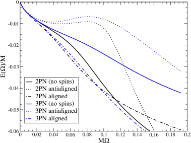
Figure 1: The energy for circular orbits as function of the frequency evaluated using the PN-expanded Hamiltonian (left panel) and the PN-expansion of the analytically computed function given by Eq. (33) (right panel) at various PN orders for maximal spins and equal mass binaries.

The most straightforward PN-based analytical approach to the physical characteristics of close BH binaries consists of starting from the fully PN-expanded Hamiltonian (15), considered as defining an exact dynamics, and then to deduce from it the energy and angular frequency of spherical orbits. [We consider here only configurations where the spins are parallel (or antiparallel) to the orbital angular momentum, so that it makes sense, even in presence of spin-spin interactions, to consider spherical (and actually circular) orbits.] The binding energy of such “PN-expanded” spherical orbits is plotted in the left panel of Fig. 1 as a function of the orbital angular frequency, for equal-mass BH binaries. As we see from this Figure, the straightforward PN-expanded Hamiltonian does not exhibit any minimum of the binding energy, i.e. does not lead to any Last Stable Spherical Orbit (LSSO) in the non-spinning, or aligned maximally spinning cases. As the best current numerical results on BH binaries clearly indicate the existence of such LSSO’s, this disqualifies the use of the fully PN-expanded Hamiltonian (15) for describing close binaries.

It has, however, been pointed out LB that more reasonable results, close to the numerical HKV results, can be obtained by plotting, instead of the prediction coming straightforwardly from (15), the PN-expansion of the analytically computed function ${E}(\Omega)$ giving the binding energy $E$ as a function of the orbital frequency $\Omega$. Indeed, one can derive from (15) the following explicit PN-expansion of the (invariant) function ${E}(\Omega)$ DJSinvar , DJS , LB :

$$E_{\rm 2PN}(\Omega) = -\frac{\mu}{2}\,(M\Omega)^{2/3}\,\left\{1-\frac{(9+\eta)}{12}\,(M\Omega)^{2/3}+\frac{8}{3}\frac{\mbox{\boldmath${\hat{L}}$}\cdot\mbox{\boldmath${S}$}_{\rm eff}}{M^{2}}\,(M\Omega)+\frac{1}{24}(-81+57\eta-\eta^{2})\,(M\Omega)^{4/3}\right.$$ (33)

$$\left.+\frac{1}{\eta}\,\frac{1}{M^{4}}\,\left[\mbox{\boldmath${S}$}_{1}\cdot\mbox{\boldmath${S}$}_{2}-3(\mbox{\boldmath${\hat{L}}$}\cdot\mbox{\boldmath${S}$}_{1})(\mbox{\boldmath${\hat{L}}$}\cdot\mbox{\boldmath${S}$}_{2})\right]\,(M\Omega)^{4/3}\right\}\,,$$

$$E_{\rm 3PN}(\Omega) = E_{\rm 2PN}(\Omega)-\frac{\mu}{2}\,(M\Omega)^{2/3}\,\left\{\left[-\frac{675}{64}+\left(\frac{34445}{576}-\frac{205}{96}\pi^{2}\right)\eta-\frac{155}{96}\eta^{2}-\frac{35}{5184}\eta^{3}\right]\,(M\Omega)^{2}\right\}\,.$$ (34)

These functions are plotted in the right panel of Fig. 1. Visibly, they are much better behaved than the results plotted on the left panel, which came directly from the PN-expanded Hamiltonian. They are also close to the numerical HKV results LB . The fact that two expressions, which can both be called “PN-expanded”, and which are supposedly equivalent “modulo higher PN terms”, lead to physically markedly different results lead to conclude that the PN-expanded Hamiltonian cannot be used to describe the transition from adiabatic inspiral to plunge. Let us also recall that if we consider, in absence of spins, the test-mass limit $\eta\to 0$, instead of the equal-mass one $\eta\to 1/4$, the PN-expansions (33),(34) have been shown (see DJS ) to be quite inaccurate representations of the known exact expression of the function ${E}(\Omega)$. Indeed, the 2PN-accurate function (33) predicts in this limit an LSO frequency which is $82\%$ larger than the exact one, while the 3PN-accurate one (34) predicts an LSO frequency $27\%$ larger than the exact one.

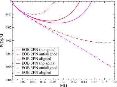
Figure 2: The energy for circular orbits as function of the frequency evaluated from the EOB Hamiltonian at various PN orders for maximal spins and equal mass binaries.

By contrast with these problematic features of PN-expanded results , the EOB-approach leads to uniformly better behaved results (even if we use it not in the Kerr-like form advocated in TD , but in the form (16) used in the present paper). We show in Fig. 2 the EOB analog of Fig. 1, i.e. the function ${E}(\Omega)$ deduced from the EOB Hamiltonian (16) in the (anti-)aligned case. In this EOB case, we have none of the problems entailed by the “PN-expanded” approach, and the uniquely defined curve ${E}(\Omega)$ was shown in DGG to agree well with the HKV numerically determined curve (for corotating holes). Note, however, that aligned maximally rotating holes lead to a curve which, especially in the 3PN case, reaches a minimum (not shown on Figure 2) only for a rather high angular velocity.

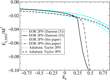
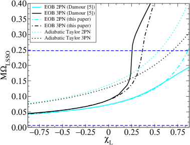
Figure 3: The energy (left panel) and the frequency (right panel) at the LSSO as function of $\chi_{L}/M^{2}\equiv S_{\rm eff}\cdot\mbox{\boldmath${\hat{L}}$}/M^{2}$ in the equal mass case for EOB Hamiltonian and PN-expanded analytically computed function ${E}(\Omega)$ [see right panel of Fig. 1]. The horizontal dashed line in the right panel marks the highest LSSO angular frequency for BBHs with total mass in the range $10\mbox{--}40M_{\odot}$, assuming the LIGO frequency band $40\leq f_{\rm GW}\leq 240Hz$.

This property of the aligned configurations (as well as the significant difference between the 2PN-EOB result and the 3PN-EOB one) was already emphasized in TD . As it will be important for the present paper, we study it further by plotting in Fig. 3 the dependence on the ${L}$- projected effective spin parameter

$$\chi_{L}\equiv\frac{\mbox{\boldmath${S}$}_{\rm eff}\cdot\mbox{\boldmath${\hat{L}}$}}{M^{2}}$$ (35)

(where $\mbox{\boldmath${S}$}_{\rm eff}$ was defined in Eq. (17) above) of the binding energy $E$ and the angular frequency $\Omega$ at the LSSO, i.e. at the minimum of the ${E}(\Omega)$ curve. This Figure shows four results obtained for equal-mass and equal-spin configurations within the EOB approach: (i) the result obtained from the Hamiltonian (16) when using the 2PN-accurate orbital EOB Hamiltonian, (ii) the result obtained from (16) when using the 3PN-accurate orbital EOB Hamiltonian, (iii) the result obtained from the 2PN-accurate Kerr-like Hamiltonian introduced in TD , and (iv) the result obtained from the 3PN-accurate Kerr-like Hamiltonian introduced in TD . [The latter two Hamiltonians are referred to in the caption as “SO Resummed”, because they include a resummation à la EOB of the spin-orbit interactions.] In addition, as we cannot show on this plot the minimum of the ${E}(\Omega)$ curve deduced from the PN-expanded Hamiltonian, because the left panel of Fig. 3 shows that it does not exist, we show instead, for comparison purposes, the characteristics of the minimum of the PN-expanded functions (33), (34) [i.e. the right panel of Fig. (1)].

It is interesting to note on Fig. 3 that the effect of resumming (à la Kerr) or not the spin-orbit interaction seems to be rather small. We see also that, when considering anti-aligned configurations, all calculations give very similar results. This is not surprising as the attractive ($H_{SO}<0$) nature of the anti-aligned spin-orbit (and spin-spin) interaction has the effect of pushing the LSSO outwards, i.e. toward larger-radius, lower-frequency, less bound and therefore less relativistic configurations. On the other hand, working at the 2PN or the 3PN level induces,as already pointed out in TD , a very significant difference for the LSSO characteristics in the aligned case (positive $\chi_{L}$). In this case, because of the repulsive($H_{SO}>0$) nature of the aligned spin-orbit (and spin-spin) interaction, the LSSO is drawn towards closer, higher-frequency, more bound and more relativistic configurations. For such very compact configurations the repulsive sign ($a_{4}>0$) of the 3PN contribution to the effective potential $A(q)$ further amplifies, by a “snow-ball effect”, the tendency toward closer, and more bound configurations. We think that this could be a physically real effect due (as confirmed independently by Refs. BDE ; Itoh ) to the large positive value of the crucial 3PN coefficient entering $a_{4}$, Eq. (14). This large positive value for $a_{4}$ is also needed to improve (with respect to the 2PN case) the agreement between the HKV corotating results and the 3PN EOB ones DGG . It would be interesting to have numerical HKV studies of the LSSO for moderately- and fast-spinning aligned BH’s to test the predictions made by the EOB approach. [The less reliable numerical results of the initial-value-problem of Ref.PTC , which extend up to mildly positive values of $\chi_{L}\sim 0.17$ are in rough qualitative agreement (especially for the dependence of $\Omega_{LSSO}$ on $\chi_{L}$) with the EOB predictions, but their quantitative agreement is too poor to reach a firm conclusion).]

Let us note in passing that the significant dependence of the LSSO frequency on the effective spin parameter $\chi_{L}$ makes it desirable for data-analysis purposes, when one is content with using adiabatic templates bcv2 , to use at least templates whose ending frequency is not fixed say to the usually considered Schwarzschild LSO, but varies with masses and spins as suggested by the EOB approach.

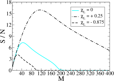
Figure 4: Signal-to-noise ratio versus binary total mass at 100 Mpc for equal-mass binaries with LSSO determined by the 3PN-EOB Hamiltonian.

Finally, another consequence of the significant dependence of the LSSO frequency on the effective spin parameter $\chi_{L}$, is drawn in Fig. 4, where we compare the signal-to-noise ratios (SNRs) as function of the binary total mass for an optimally oriented equal-mass binary at 100 Mpc. We use LIGO design sensitivity noise curve DIS98 . The SNRs are obtained observing the inspiral from 40 Hz until the LSSO predicted by the EOB approach at 3PN order. The three curves refer to non-spinning binaries and binaries with $\chi_{L}=-0.875,0.25$. Figure 4 reveals a bias towards first detecting mostly aligned spinning binaries with high masses, as pointed out in TD .

III Radiation reaction, including spin-effects

The previous section has reviewed various ways of describing the conservative dynamics of binary systems (including spin effects). In the present section, we discuss the inclusion of radiation reaction effects, with emphasis on determining the spin-modifications of radiation reaction. Within the Hamiltonian approach, that we use here, radiation reaction can be incorporated by modifying the usual Hamilton equations in the following way

$$\frac{dX^{i}}{dt}=\{X^{i},H\}=\frac{\partial H}{\partial P_{i}}\,,$$

$$\frac{dP_{i}}{dt}=\{P_{i},H\}+F_{i}=-\frac{\partial H}{\partial X^{i}}+F_{i}\,.$$ (36)

Here, $F_{i}$ denotes a “non-conservative force”, which is added to the evolution equation of the (relative) momentum to take into account radiation-reaction (RR) effects. This Radiation-Reaction (RR) force ${F}$ depends, a priori, both on the (relative) orbital variables ${X}$, ${P}$ and on the spin variables $\mbox{\boldmath${S}$}_{1}$, $\mbox{\boldmath${S}$}_{2}$. In the present paper, our aim will be limited to determining $F_{i}$ under the following two simplifying assumptions: (i) we consider only quasi-circular orbits, and (ii) we shall retain only the leading spin-dependent terms. After the completion of the work reported in this section, there appeared a work of Will Will dealing with spin-dependent radiation reaction effects in general orbits. As the derivations are not the same, and yield results which we have checked to be equivalent (for circular orbits), but expressed in different variables (Hamiltonian ${X}$, ${P}$ here vs. Lagrangian ${X}$, ${V}$ for Will ), we feel it worth to briefly report our derivation.

Because of the assumption (ii) we look for terms in $F_{i}$ which are linear in the spin-tensors $S_{ij}^{a}\equiv\varepsilon_{ijk}\,S_{a}^{k}$ ($a=1,2$) of the two considered compact bodies. [Note that spin effects enter the metric only through the spin tensors $S_{ij}^{a}$, rather than through the axial spin vectors $S_{a}^{k}$.] As the time derivative of $S_{ij}^{a}$ contains a “small” post-Newtonian factor $G/c^{2}$, the leading spin-dependent terms in $F_{i}$ will contain only the undifferentiated spin tensors.

Using Euclidean invariance, the spin-dependent terms in the force $F_{i}(\mbox{\boldmath${X}$},\mbox{\boldmath${P}$},\mbox{\boldmath${S}$}_{a})$ must be a combination of three types of contributions: $c_{1}\,S_{ij}\,X^{j}$, $c_{2}\,S_{ij}\,P^{j}$ and $c_{i}\,S_{jk}\,X^{j}P^{k}$, where $c_{1}(\mbox{\boldmath${X}$},\mbox{\boldmath${P}$})$, $c_{2}(\mbox{\boldmath${X}$},\mbox{\boldmath${P}$})$ are some scalar functions of ${X}$, ${P}$, while $c_{i}$ is a vector function of ${X}$, ${P}$. [Here, $S_{ij}$ denotes one of the two spin vectors. We shall sum over the two possible spins at the end.] Imposing that the radiation reaction force $F_{i}$ be odd under time reversal, i.e. odd under the simultaneous changes $X^{i}\to X^{i}$, $P_{i}\to-P_{i}$, $S_{ij}\to-S_{ij}$, tells us that: $c_{1}(\mbox{\boldmath${X}$},\mbox{\boldmath${P}$})$ must be an even function of ${P}$, $c_{2}(\mbox{\boldmath${X}$},\mbox{\boldmath${P}$})$ must be an odd function of ${P}$, and the vector $c_{i}(\mbox{\boldmath${X}$},\mbox{\boldmath${P}$})$ must be an odd function of ${P}$. [Note also that $c_{i}$ must be a true vector, not an axial vector. By parity invariance no $\varepsilon_{ijk}$ can appear, except in combination with $S_{a}^{k}$.] Therefore, if we further decompose $c_{i}=c_{3}(\mbox{\boldmath${X}$},\mbox{\boldmath${P}$})\,P_{i}+c_{4}(\mbox{\boldmath${X}$},\mbox{\boldmath${P}$})\,X_{i}$, the coefficient $c_{3}(\mbox{\boldmath${X}$},\mbox{\boldmath${P}$})$ must be even in ${P}$, while the coefficient $c_{4}(\mbox{\boldmath${X}$},\mbox{\boldmath${P}$})$ must be odd in ${P}$.

At this point, our simplifying assumption (i) above (quasi-circular motion) will bring a drastic simplification. Indeed, a time-odd scalar must contain an odd power of the combination $X^{k}P_{k}$. However, this combination vanishes along circular orbits (and is therefore subleadingly small along adiabatically inspiralling orbits). To leading order the scalar coefficients $c_{2}$ and $c_{4}$ therefore vanish, and we conclude that $F_{i}$ contains only two independent spin contributions: $c_{1}(\mbox{\boldmath${X}$},\mbox{\boldmath${P}$})\,S_{ij}\,X^{j}+c_{3}(\mbox{\boldmath${X}$},\mbox{\boldmath${P}$})\,P_{i}\,S_{jk}\,X^{j}P^{k}$. It will be convenient in the following to further decompose the vector $S_{ij}\,X^{j}$ entering the first contribution (which is orthogonal to $X^{i}$) into its component along the direction of $P_{i}$, and its component orthogonal to $P_{i}$, say

$$(S_{ij}\,X^{j})^{\perp}\equiv(\delta_{ik}-P_{i}\,P_{k}/\mbox{\boldmath${P}$}^{2})\,S_{kj}\,X^{j}=S_{ij}\,X^{j}+\frac{P_{i}}{\mbox{\boldmath${P}$}^{2}}\,S_{jk}\,X^{j}P^{k}\,.$$ (37)

It is easily checked that, along circular orbits $(X^{i}\,P_{i}=0)$, the vector (37) is orthogonal both to ${P}$ and to ${X}$. Therefore, $(S_{ij}\,X^{j})^{\perp}$ is parallel to the orbital angular momentum (axial) vector

$$L_{i}\equiv\varepsilon_{ijk}\,X^{j}\,P_{k}\,.$$ (38)

It is easily checked that

$$(S_{ij}\,X^{j})^{\perp}=\frac{R^{2}}{\mbox{\boldmath${L}$}^{2}}\,(\mbox{\boldmath${P}$}\cdot\mbox{\boldmath${S}$})\,L_{i}=\frac{1}{\mbox{\boldmath${P}$}^{2}}\,(\mbox{\boldmath${P}$}\cdot\mbox{\boldmath${S}$})\,L_{i}\,.$$ (39)

Finally, adding the usual spin-independent radiation reaction (parallel to $P_{i}$ for circular orbits), and summing over the two bodies, we conclude that the RR force can be written as

$$F_{i}(\mbox{\boldmath${X}$},\mbox{\boldmath${P}$},\mbox{\boldmath${S}$}_{a})=B\,P_{i}+\sum_{a=1,2}A_{a}(S_{ij}^{a}\,X^{j})^{\perp}=B\,P_{i}+\sum_{a=1,2}\frac{A_{a}}{\mbox{\boldmath${P}$}^{2}}\,(\mbox{\boldmath${P}$}\cdot\mbox{\boldmath${S}$}_{a})\,L_{i}\,,$$ (40)

with

$$B\equiv B_{0}+\sum_{a=1,2}C_{a}\,S_{jk}^{a}\,X^{j}P^{k}=B_{0}+\sum_{a=1,2}C_{a}\,\mbox{\boldmath${L}$}\cdot\mbox{\boldmath${S}$}_{a}\,,$$ (41)

where $B_{0}$, $C_{a}$ and $A_{a}$ are some time-even functions of ${X}$ and ${P}$.

To determine the coefficients $B_{0}$, $C_{a}$ and $A_{a}$, we now impose that there be a balance between the losses of mechanical energy and angular momentum of the system due to the additional force $F_{i}$ in the Hamilton equations of motion (36) and the losses of energy and angular momentum at infinity due to the emission of gravitational radiation. Let us first recall that, in the Hamiltonian formalism, the quantities

$$E(t)\equiv H(\mbox{\boldmath${X}$}(t),\mbox{\boldmath${P}$}(t),\mbox{\boldmath${S}$}_{a}(t))\,,$$

$$J_{ij}(t)\equiv X^{i}\,P_{j}-X^{j}\,P_{i}+S_{ij}^{1}+S_{ij}^{2}\,,$$ (42)

are exact constants of the motion in absence of RR force in Eqs. (36) and in the Hamiltonian equations for spin evolution. When adding the RR force ${F}$ in Eqs. (36) (and no corresponding RR torque in the spin evolution equations) we find that $E$ and ${J}$ evolve as

$$\frac{dE}{dt}=\frac{\partial H}{\partial P_{i}}\,F_{i}=\dot{X}^{i}\,F_{i}\,,$$ (43)

$$\frac{d\,J_{ij}}{dt}=X^{i}\,F_{j}-X^{j}\,F_{i}\,.$$ (44)

Inserting in Eqs. (43,44) the expression (40) for the RR force $F_{i}$, we can easily evaluate the averaged losses of energy and angular momentum. Along (quasi) circular orbits the various scalar coefficients $B_{0}$, $C_{a}$, $A_{a}$ are time-independent (because all basic scalars, $\mbox{\boldmath${X}$}^{2},\mbox{\boldmath${P}$}^{2},\mbox{\boldmath${X}$}\cdot\mbox{\boldmath${P}$}=0$, are constant). One then finds that $dE/dt$ is time-independent, while $d\,J_{ij}/dt$ depends on the orbital phase only in spin-dependent terms and through the tensor $X^{i}\,P_{j}$. Decomposing the latter tensor into

$$X^{i}\,P_{j}=\frac{1}{2}(X^{i}\,P_{j}+X^{j}\,P_{i})+\frac{1}{2}(X^{i}\,P_{j}-X^{j}\,P_{i})\simeq\frac{d}{dt}\left(\frac{1}{2}\,\mu\,X^{i}\,X^{j}\right)+\frac{1}{2}\,L_{ij}\,,$$ (45)

one easily sees that its orbital average is simply $\langle X^{i}\,P_{j}\rangle=\frac{1}{2}\,L_{ij}$. [We consider averages over the orbital period, considering all more slowly evolving quantities, such as ${L}$, as fixed during one orbital period.]

When evaluating Eq. (43) along circular orbits, we cannot use the Newtonian approximation $\dot{X}^{i}\simeq P^{i}/\mu$ because we wish to obtain the coefficient $B$ with a high post-Newtonian accuracy. However we can instead use $\dot{X}^{i}\,P_{i}=\dot{\phi}\,P_{\phi}=\omega\,|\mbox{\boldmath${L}$}|$ where $\omega=\dot{\phi}=V/R$ denotes the orbital angular frequency. We finally obtain

$$\frac{dE}{dt}=B\,\omega\,|\mbox{\boldmath${L}$}|\,,$$ (46)

$$\left\langle\frac{d\mbox{\boldmath${J}$}}{dt}\right\rangle=B\,\mbox{\boldmath${L}$}-\frac{1}{2}\sum_{a=1,2}A_{a}\,R^{2}\,[\mbox{\boldmath${S}$}_{a}-\mbox{\boldmath${\lambda}$}(\mbox{\boldmath${\lambda}$}\,\mbox{\boldmath${S}$}_{a})]\,,$$ (47)

where $\mbox{\boldmath${\lambda}$}\equiv\mbox{\boldmath${L}$}/|\mbox{\boldmath${L}$}|$ denotes the unit vector along the orbital angular momentum. Note that Eqs. (46), (47) predict a link between energy loss and angular momentum loss, namely

$$\frac{dE}{dt}=\omega\,\mbox{\boldmath${\lambda}$}\cdot\left\langle\frac{d\mbox{\boldmath${J}$}}{dt}\right\rangle\,.$$ (48)

To obtain the values of the coefficients $B$ and $A_{a}$ (and to test the prediction (48)), we need to compare Eqs. (46), (47) with the values of the averaged fluxes of energy and angular momentum at infinity. The spin contributions to the latter losses have been computed by Kidder K . However, one must be careful with the fact that Kidder expressed most of his results in terms of harmonic coordinates, with the choice of a covariant spin supplementary condition: $S_{\mu\nu}^{a}\,u_{a}^{\nu}=0$.

First, using the results of Ref. K as they are, one straightforwardly checks that the relation (48) is satisfied. This is a check that it is enough to include RR effects in the orbital equations of motion (36), without modifying the spin equations of motion. [For a direct dynamical check, see Will .] Then, to obtain the value of the coefficient $B$ we can simply use the result (46), namely

$$B=\frac{1}{\omega\,|\mbox{\boldmath${L}$}|}\ \frac{dE}{dt}\,,$$ (49)

where it remains to express $dE/dt$ (computed as a flux at infinity, using Ref. K ) in terms of our basic (Hamiltonian) dynamical variables. One way to proceed would be to transform the harmonic-coordinates results of K into ADM coordinates (with the corresponding spin condition $S_{i0}+\frac{1}{2}\,S_{ij}\,v^{j}=0$ DS88 ). The transformation linking the two coordinates has been worked out in DS88 (for the spin-dependent terms) and in DJS01 ; ABF01 for the spin-independent parts. However, a simpler way to proceed is to eliminate references to specific coordinates by expressing $dE/dt$ (for circular orbits) in terms of the gauge-invariant orbital frequency $\omega$. Adding also, for better accuracy the recently completed 3PN flux contribution BIJ02 ; B98 ; BDEI04 , we have

$$\frac{dE}{dt}=-\frac{32}{5}\,\eta^{2}\,v_{\omega}^{10}\{1+f_{2}(\eta)\,v_{\omega}^{2}+[f_{3}(\eta)+f_{3{\rm SO}}]\,v_{\omega}^{3}+[f_{4}(\eta)+f_{4{\rm SS}}]\,v_{\omega}^{4}+f_{5}(\eta)\,v_{\omega}^{5}+f_{6}(\eta)\,v_{\omega}^{6}+f_{\ell 6}\,v_{\omega}^{6}\,\ln(4v_{\omega})+f_{7}(\eta)\,v_{\omega}^{7}\}\,,$$ (50)

where $v_{\omega}\equiv(GM\omega)^{1/3}$, where the spin-independent flux coefficients $f_{2}(\eta),\ldots,f_{7}(\eta)$, are given by

$$f_{2}(\eta)=-\frac{1247}{336}-\frac{35}{12}\,\eta\,,$$ (51)

$$f_{3}(\eta)=4\pi\,,$$ (52)

$$f_{4}(\eta)=-\frac{44711}{9072}+\frac{9271}{504}\eta+\frac{65}{18}\eta^{2}\,,\quad\quad f_{5}(\eta)=-\left(\frac{8191}{672}+\frac{583}{24}\eta\right)\pi\,,$$ (53)

$$f_{6}(\eta)=\frac{6643739519}{69854400}+\frac{16}{3}\,\pi^{2}-\frac{1712}{105}\,\gamma_{E}+\left(-\frac{134543}{7776}+\frac{41}{48}\,\pi^{2}\right)\eta-\frac{94403}{3024}\,\eta^{2}-\frac{775}{324}\,\eta^{3}\,,$$ (54)

$$f_{\ell 6}=-\frac{1712}{105}$$ (55)

$$f_{7}(\eta)=\left(-\frac{16285}{504}+\frac{214745}{1728}\eta+\frac{193385}{3024}\eta^{2}\right)\,\pi\,,$$ (56)

with $\gamma_{E}$ being Euler’s gamma, and where the spin-dependent corrections to the latter flux coefficients are

$$f_{3{\rm SO}}=-\left(\frac{11}{4}+\frac{5}{4}\,\frac{m_{2}}{m_{1}}\right)\frac{\mbox{\boldmath${\lambda}$}\cdot\mbox{\boldmath${S}$}_{1}}{GM^{2}}-\left(\frac{11}{4}+\frac{5}{4}\,\frac{m_{1}}{m_{2}}\right)\frac{\mbox{\boldmath${\lambda}$}\cdot\mbox{\boldmath${S}$}_{2}}{GM^{2}}\,,$$ (57)

$$f_{4{\rm SS}}=\frac{\eta}{48G^{2}m_{1}^{2}\,m_{2}^{2}}\,[289(\mbox{\boldmath${\lambda}$}\cdot\mbox{\boldmath${S}$}_{1})(\mbox{\boldmath${\lambda}$}\cdot\mbox{\boldmath${S}$}_{2})-103\,\mbox{\boldmath${S}$}_{1}\cdot\mbox{\boldmath${S}$}_{2}]+\mathcal{O}(\mbox{\boldmath${S}$}_{1}^{2})+\mathcal{O}(\mbox{\boldmath${S}$}_{2}^{2})\,.$$ (58)

The present work was aimed at determining the leading spin-dependent terms, i.e. the ones linear in $\mbox{\boldmath${S}$}_{1}$ and $\mbox{\boldmath${S}$}_{2}$, as exemplified in the correction $f_{3{\rm SO}}$, Eq. (57), to the coefficient $f_{3}=4\pi$. For completeness, as the link (49) between the “longitudinal” part of RR, $F_{i}^{\rm long}=B\,P_{i}$, and the energy loss, is clearly general, we have also used Kidder’s results K to write down the part of $B$ which depends on the product $\mbox{\boldmath${S}$}_{1}^{i}\,\mbox{\boldmath${S}$}_{2}^{j}$. The numerically similar contributions which depend on $\mbox{\boldmath${S}$}_{1}^{i}\,\mbox{\boldmath${S}$}_{1}^{j}$ and $\mbox{\boldmath${S}$}_{2}^{i}\,\mbox{\boldmath${S}$}_{2}^{j}$ have not yet been determined. Only partial results are known. For instance, Poisson EP has derived a contribution to $f_{4{\rm SS}}$ of the form

$$\left[\frac{3(\mbox{\boldmath${\lambda}$}\cdot\mbox{\boldmath${S}$}_{1})^{2}-\mbox{\boldmath${S}$}_{1}^{2}}{G^{2}m_{1}^{2}\,M^{2}}+\frac{3(\mbox{\boldmath${\lambda}$}\cdot\mbox{\boldmath${S}$}_{2})^{2}-\mbox{\boldmath${S}$}_{2}^{2}}{G^{2}m_{2}^{2}M^{2}}\right]\,.$$ (59)

but many other additional contributions $\mathcal{O}(\mbox{\boldmath${S}$}_{1}^{2})+\mathcal{O}(\mbox{\boldmath${S}$}_{2}^{2})$ have not yet been computed.

Let us finally turn to the determination of the other spin-related coefficients, $A_{a}$, in Eq. (47). Again, we have the technical problem that Ref. K expressed its results in terms of harmonic-coordinate quantities. Namely, Eq. (4.11) of Ref. K expresses the total angular momentum loss $d\mbox{\boldmath${J}$}/dt$ in terms of the harmonic distance $r$ and of the harmonic-coordinate “Newtonian orbital momentum” $\mbox{\boldmath${L}$}_{N}\equiv\mu\,\mbox{\boldmath${x}$}\times\mbox{\boldmath${v}$}$ (where ${x}$ and ${v}$ denote the relative harmonic position and velocity). A simple way to convert this result to our ADM distance $R$ and our ADM total orbital momentum $\mbox{\boldmath${L}$}\equiv\mbox{\boldmath${X}$}\times\mbox{\boldmath${P}$}$ is to relate $\mbox{\boldmath${L}$}_{N}$ to ${L}$ by comparing the expression (4.7) of Ref. K for the (gauge-invariant) conserved total angular momentum ${J}$ with the corresponding simple ADM expression (42). This yields a result of the form

$$\hat{}\mbox{\boldmath${L}$}_{N}\equiv\frac{\mbox{\boldmath${L}$}_{N}}{|\mbox{\boldmath${L}$}_{N}|}=c\,\mbox{\boldmath${L}$}+\left(\frac{GM}{r}\right)^{\frac{3}{2}}\sum_{a=1,2}\chi_{a}\,\hat{}\mbox{\boldmath${s}$}_{a}\left(\frac{m_{a}^{2}}{M^{2}}+\frac{1}{4}\,\eta\right)\,,$$ (60)

where the coefficient $c$ is not needed for our present purpose, and where, following the notation of K , $\mbox{\boldmath${S}$}_{a}\equiv\chi_{a}\,m_{a}^{2}\,\hat{}\mbox{\boldmath${s}$}_{a}$. Inserting Eq. (60) in Eq. (4.11) of K allows one to compute easily the part of $d\mbox{\boldmath${J}$}/dt$ which is proportional to the projection of $\mbox{\boldmath${S}$}_{a}$ orthogonally to ${L}$.

This yields the following expression for the coefficients $A_{a}$ in Eq. (40)

$$A_{a}=\frac{8}{15}\,\eta^{2}\,\frac{v_{\omega}^{8}}{R^{3}}\left(61+48\,\frac{m_{a^{\prime}}}{m_{a}}\right)\,,$$ (61)

where $a^{\prime}\neq a$ (e.g. $a^{\prime}=2$ when $a=1$). Summarizing, the radiation reaction force to be added to the Hamiltonian equations of motion (36) reads

$$F_{i}=\frac{1}{\omega\,|\mbox{\boldmath${L}$}|}\,\frac{dE}{dt}\,P_{i}+\frac{8}{15}\,\eta^{2}\,\frac{v_{\omega}^{8}}{\mbox{\boldmath${L}$}^{2}R}\left\{\left(61+48\,\frac{m_{2}}{m_{1}}\right)\mbox{\boldmath${P}$}\cdot\mbox{\boldmath${S}$}_{1}+\left(61+48\,\frac{m_{1}}{m_{2}}\right)\mbox{\boldmath${P}$}\cdot\mbox{\boldmath${S}$}_{2}\right\}L_{i}\,,$$ (62)

where the energy loss (expressed in terms of the orbital frequency $\omega$, or equivalently of $v_{\omega}\equiv(GM\omega)^{1/3}$, and of the spin variables) is given by Eqs. (50)–(58). We have checked that, after taking into account the relation between the Hamiltonian variables $\mbox{\boldmath${X}$},\mbox{\boldmath${P}$}$ and the Lagrangian ones $\mbox{\boldmath${X}$},\mbox{\boldmath${V}$}$ (which involves spin-dependent terms because of the first Eq. (23), Eq. (62) agrees with the circular limit of Eq. (1.6) of Will (which assumes the same spin condition as we do).

Refs. DIS98 ; BD2 ; DIS01 ; PS have shown that (at least in the test-mass limit where one can compare analytical and numerical estimates) it is generally advantageous to replace the Taylor series in curly brackets on the right hand side (R.H.S.) of Eq. (50) by its (suitably defined) Padé resummation. In particular, Porter and Sathyaprakash PS have compared “Taylor” and “Padé” approximants for the flux function of a test particle around a Kerr black hole with the exact numerical estimates fluxS and concluded that Padé approximants are, when considering all values of the spin parameter, both more effectual (i.e., larger overlaps with the exact signal) and more faithful (i.e., smaller biases in parameter estimates) than Taylor approximants. [We use here the terminology introduced in DIS98 .] In view of this, and as was already advocated in BD2 , we consider that that the best way to incorporate a radiation reaction force in the EOB approach is to insert Padé approximants of the flux function (R.H.S. of (50)) in (62). However, for added generality, we shall also consider the case where we leave the flux function as a plain Taylor series. Note that, when considering arbitrary values of the dimensionless spin parameters for the two holes $\chi_{1}\equiv S_{1}/Gm_{1}^{2}$, $\chi_{2}\equiv S_{2}/Gm_{2}^{2}$ we used the normal “direct” (i.e., lower-diagonal) Padé-approximants, instead of the “inverse”(i.e., upper-diagonal) ones used in PS . For some values of the spin parameters both the lower and upper diagonal Padé-approximants have poles. When this occurs, we apply the Padé-approximant only to the non-spinning part of the flux and add the spinning terms separately. There exist other Padé-approximants in which poles are absent and it would be very desirable to determine them in the entire parameter space. This is beyond the scope of this paper.

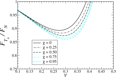
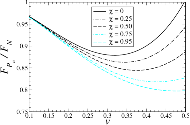
Figure 5: Newton-normalized flux in the equal-mass case with both BH spins aligned (and maximal $\chi=\chi_{1}=\chi_{2}$) with orbital angular momentum when T-approximants (left panel) and (upper-diagonal) P-approximants (right panel) are used.

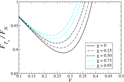
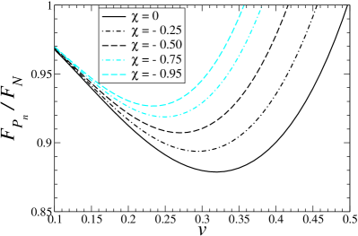
Figure 6: Newton-normalized flux in the equal-mass case with both BH spins antialigned (and maximal $\chi=\chi_{1}=\chi_{2}$) with orbital angular momentum when T-approximants (left panel) and (upper-diagonal) P-approximants (right panel) are used.

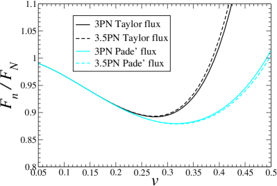
Figure 7: Comparison between the T- and (upper diagonal) P-approximant Newton-normalized flux in the equal mass case at 3PN and 3.5PN order.

In Figs. 5, 6 we show T- and (lower-diagonal) P-approximants at 3.5PN order for an equal-mass binary and several values of the dimensionless spin parameter $\chi=\chi_{1}=\chi_{2}$. We notice that the T- and P-approximants are much closer in the anti-aligned cases than in the aligned one. Since the calculation of the non-spinning flux function at 3.5PN order has been completed only recently BDE , in Fig. 7 we contrast the T- and (lower-diagonal) P-approximants at 3PN and 3.5PN order for an equal-mass non-spinning binary.

IV Definitions of the initial and ending conditions of two-body models

As clear from the comparison of the left and right panel of Fig. 1, because of the bad behaviour of the PN Hamiltonian near LSSO, we propose as our best bet, for describing in a physically reliable manner the non-adiabatic evolution of BH binaries, and their transition between inspiral and plunge, to use an EOB-resummed Hamiltonian, we shall, for more generality, consider, and compare, in this Section several types of two-body models.

To define a specific model we must make various choices: (i) choice of a PN-expanded (or “Taylor-expanded”) Hamiltonian (say “TH”) versus an EOB-resummed Hamiltonian (say “EH”); (ii) choice of a Taylor-expanded flux function (say “TF”) versus a Padé-resummed one (say “PF”), and finally, (iii) choice of the PN accuracies used both in the Hamiltonian (say $n$ PN) and the flux function (say $m$ PN). This leads to models denoted, for instance,${\rm THTF}(n,m)$, ${\rm EHTF}(n,m)$, ${\rm EHPF}(n,m)$. In addition, as we are here mainly considering the evolution of spinning binaries, we shall add an initial letter S to recall that fact. This leads to models denoted as ${\rm STHTF}(n,m)$,…, ${\rm SEHPF}(n,m)$. To simplify, we shall only consider the PN accuracies $(2,2.5)$ or $(3,3.5)$. To further simplify, we shall focus on comparing “fully Taylor” models (i.e., ${\rm STHTF}$), to “fully resummed ” ones (i.e., ${\rm SEHPF}$). Finally, this leads us to considering only four models: ${\rm STHTF(2,2.5)}$, ${\rm STHTF}(3,3.5)$, ${\rm SEHPF}(2,2.5)$, and ${\rm SEHPF}(3,3.5)$. [Note, as discussed above, that because of the appearance of spurious poles in a few tests, we applied in those cases, the Pade resummation only to the non-spinning part of the flux.]

An important parameter in our present model building is to decide when to stop the evolution. This issue was already tackled in Ref. BD2 . There, because we were using an EOB Hamiltonian, and were considering non-spinning BH’s, we found that we could follow the “plunge” (after LSO crossing) down to a (Schwarzschild-like) radius $\simeq 3M$, at which point we could match to a ring-down signal made of least-damped quasi-normal modes. It was found in BD2 that, contrary to what the usually employed word “plunge” suggests, the inspiral motion after crossing the LSO was staying “quasi-circular”, with a kinetic energy in the radial motion staying small in absolute value, and smaller than $0.3$ times the kinetic energy in the azimuthal motion down to $R\simeq 3M$. In our “spinning” evolutions the situation is more complicated (notably when considering large aligned spins, and also, for evident reasons, when considering Taylor-expanded Hamiltonians). We leave to future work a detailed discussion of the matching to ring-down. We decided to stop the evolution as soon as one of the following inequalities ceased to be fulfilled:

$$|\dot{R}| < 0.3|\mathbf{V}_{t}|\,,$$ (63a)

$$P_{R}^{2}/B(R) < 0.3P^{2}_{\phi}/R^{2}\,,$$ (63b)

$$|\dot{E}_{RR}| > 0.1|\dot{E}_{RR}^{\rm Newt}|\,,$$ (63c)

$$R > \alpha M\,,$$ (63d)

where $B(R)=D(R)/A(R)$ [see Eqs. (13), (12)]. Criteria (63a)–(63b) ensure that the evolution does not extend too much beyond circularity, on which our formulation for radiation-reaction force relies. The quantity $\mathbf{V}_{t}$ is the tangential velocity (i.e., orthogonal to the relative separation vector $\mathbf{X}$). Criterion (63c) is used to avoid going into regimes where the GW energy flux goes to zero (e.g., for Taylor-expanded flux at 2.5PN order). Criterion (63d) (in which $\alpha\sim 1$ when using the ADM-coordinate Taylor-expanded Hamiltonian, and $\alpha\sim 2$ when using the Schwarzschild-like EOB Hamiltonian) terminates the evolution at a very small radius, in case all of the above criteria fail to take effect.

In all cases, the instantaneous GW frequency at the time when the integration is stopped defines the ending frequency for these waveforms. We shall also consider below extended waveforms obtained by matching a ring-down signal when this ending frequency is reached.

IV.1 Initial conditions: quasi-spherical orbits

[In this section we shall use natural units $c=1=G$ and set $M=1$.]

In absence of radiation reaction (RR), spherical orbits with constant radius and orbital frequency exists under spin-orbit interactions, but cease to exist when spin-spin interactions are present (except in special situations when the spins and the orbital angular momentum are all aligned/anti-aligned). When radiation reaction is treated adiabatically, an initial spherical orbit will evolve into a sequence of spherical orbits, due to Eq. (48). In this section, we formulate a prescription to construct initial conditions for non-adiabatic evolutions, which lead to quasi-spherical orbits under spin-orbit interaction.

With spin terms kept only up to the spin-orbit order, the Hamiltonian can be re-written into a simpler form,

$$H(R,P_{R},L,\chi_{L})=H_{\rm no\,spin}(R,P_{R},L)+2\frac{L\chi_{L}}{R^{3}}\,.$$ (64)

Here $H_{\rm no\,spin}$ are terms in the Hamiltonian that do not involve spins, and

$$L\equiv|\mathbf{L}|\,,\quad\chi_{L}\equiv\mathbf{S}_{\rm eff}\cdot\hat{\mathbf{L}}.$$ (65)

In this form, the Hamiltonian depends on four quantites, $\{R,P_{R},L,\chi_{L}\}$, in which $L$ and $\chi_{L}$ both depend on $\{\theta,\phi,P_{\theta},P_{\phi}\}$, while $\chi_{L}$ also depends on the spins. In absence of radiation reaction, the conditions for spherical orbits written in terms of partial derivatives (indicated by a subscript $i$) with respect to the four independent variables $\{R,P_{R},L,\chi_{L}\}$, read

$$\big{[}\dot{R}\big{]}_{0}=0 \Rightarrow \left[P_{R}\right]_{0}=0\,,$$ (66)

$$\big{[}\dot{P}_{R}\big{]}_{0}=0 \Rightarrow \left[\left(\frac{\partial H}{\partial R}\right)_{c}\right]_{0}=\left[\left(\frac{\partial H}{\partial R}\right)_{i}\right]_{0}=0\,.$$ (67)

[Here the subscript $c$ indicates canonical partial derivatives. In the rest of this section, we shall continue to use $i$ and $c$ to distinguish between these two types of partial derivatives.] With $L$ and $\chi_{L}$ being conserved quantities, conditions (66) and (67) will remain satisfied if they are initially satisfied — which proves the existence of spherical orbits.

We now construct initial conditions for spherical orbits, in absence of radiation reaction, based on Eqs. (66) and (67). In numerical evolutions, given a source coordinate frame, $\{\mathbf{e}_{x},\mathbf{e}_{y},\mathbf{e}_{z}\}$, we specify spherical orbits with the following initial kinetic parameters: the orbital frequency $\omega_{0}$, the orbital orientation (i.e., the normal direction to the orbital plane $[\hat{\mathbf{L}}_{\rm N}]_{0}=(\mbox{\boldmath${X}$}\times\dot{\mbox{\boldmath${X}$}})/|\mbox{\boldmath${X}$}\times\dot{\mbox{\boldmath${X}$}}|$), the spins $[\mathbf{S}_{1,2}]_{0}$, and the direction of initial orbital separation $\mathbf{N}=\mbox{\boldmath${X}$}/|\mbox{\boldmath${X}$}|$, which can in turn be given by an initial orbital phase $\phi_{\rm orb}$, calculated with respect to the reference direction of $[\mathbf{S}_{\rm tot}\times\hat{\mathbf{L}}_{\rm N}]_{0}$,

$$\mathbf{N}_{0}=\frac{[\mathbf{S}_{\rm tot}\times\hat{\mathbf{L}}_{\rm N}]_{0}}{|[\mathbf{S}_{\rm tot}\times\hat{\mathbf{L}}_{\rm N}]_{0}|}\cos\phi_{\rm orb}+\frac{[\hat{\mathbf{L}}_{\rm N}]_{0}\times[\mathbf{S}_{\rm tot}\times\hat{\mathbf{L}}_{\rm N}]_{0}}{|[\mathbf{S}_{\rm tot}\times\hat{\mathbf{L}}_{\rm N}]_{0}|}\sin\phi_{\rm orb}\,.$$ (68)

We calculate initial values for $\{\mathbf{X},\mathbf{P}\}$ in three steps:

1. We first apply a rotation $\mathcal{R}$ such that $[\hat{\mathbf{L}}_{\rm N}]_{0}\rightarrow\mathbf{e}_{z}$ and $\mathbf{N}_{0}\rightarrow\mathbf{e}_{x}$.

2. In spherical polar coordinates, the above step implies

   $$\phi_{0}=0\,,\;\;\;\;\theta_{0}=\pi/2\,.$$ (69)

   [The $\phi_{0}$ here should not to be confused with the orbital phase $\phi_{\rm orb}$ above.] Then, we specify the initial frequency $\omega_{0}$ and impose

   $$\omega_{0}=\dot{\phi}_{0}=\left[\left(\frac{\partial H}{\partial P_{\phi}}\right)_{c}\right]_{0}\,, 0=\dot{\theta}_{0}=\left[\left(\frac{\partial H}{\partial P_{\theta}}\right)_{c}\right]_{0};$$ (70)

   $$\left[P_{R}\right]_{0}=0\,, \left[\left(\frac{\partial H}{\partial R}\right)_{c}\right]_{0}=0\,,$$ (71)

   and solve for the four variables $\{R,P_{R},P_{\theta},P_{\phi}\}_{0}$.

3. Finally, we apply the inverse rotation $\mathcal{R}^{-1}$ to the entire system, obtaining a set of initial spherical-orbit conditions consistent with the specified initial kinetic parameters.

When radiation reaction is included, we proceed as in Ref. BD2 and modify Eq. (66) to include a non-zero $\dot{R}$, according to the prediction from adiabatic evolution,

$$\big{[}\dot{R}\big{]}_{0}=\left[\frac{\dot{E}_{\rm RR}}{(dE/dR)_{\rm sph}}\right]_{0}\,,$$ (72)

in order to prevent radial oscillations. [The subscript sph in Eq. (72) and below denote quantities evaluated along spherical orbits.] Equations (67) can be kept unchanged, since $\dot{P}_{R}$ is second order in radiation reaction. We now calculate $(dE/dR)_{\rm sph}$ in terms of the simplified set of independent variables, $\{R,P_{R},L,\chi_{L}\}$. Consider neighboring spherical orbits in an adiabatic sequence, we have

$$dH=\left(\frac{\partial H}{\partial R}\right)_{i}dR+\left(\frac{\partial H}{\partial P_{R}}\right)_{i}dP_{R}+\left(\frac{\partial H}{\partial L}\right)_{i}dL+\left(\frac{\partial H}{\partial\chi_{L}}\right)_{i}d\chi_{L}\,,$$ (73)

$$\left(\frac{\partial H}{\partial R}\right)_{i}=0,\;\;d\left(\frac{\partial H}{\partial R}\right)_{i}=0,\;\;P_{R}=0,\;\;dP_{R}=0\,.$$ (74)

It is straightforward to deduce that

$$\left(\frac{dE}{dR}\right)_{\rm sph}=-\frac{\displaystyle\bigg{(}\frac{\partial H}{\partial L}\bigg{)}_{i}\bigg{(}\frac{\partial^{2}H}{\partial R^{2}}\bigg{)}_{i}}{\displaystyle\bigg{(}\frac{\partial^{2}H}{\partial R\partial L}\bigg{)}_{i}}+\underbrace{\left[\left(\frac{\partial H}{\partial\chi_{L}}\right)_{i}-\frac{\displaystyle\bigg{(}\frac{\partial H}{\partial L}\bigg{)}_{i}\bigg{(}\frac{\partial^{2}H}{\partial R\partial\chi_{L}}\bigg{)}_{i}}{\displaystyle\bigg{(}\frac{\partial^{2}H}{\partial R\partial L}\bigg{)}_{i}}\right]\left(\frac{d\chi_{L}}{dR}\right)_{\rm sph}}_{\mbox{will be ignored}}\,.$$ (75)

The second term on the right-hand side can be ignored, as we argue later in this section, because $\chi_{L}$ is still conserved to a high accuracy even in presence of radiation reaction. In special configurations with $\hat{\mathbf{L}}=\mathbf{e}_{z}$ (or equivalently $\theta=\pi/2$, $P_{\theta}=0$) we can re-write Eq. (75) in terms of canonical variables in spherical-polar coordinates:

$$\left(\frac{dE}{dR}\right)_{\rm sph}=-\left[\frac{(\partial H/\partial P_{\phi})_{c}(\partial^{2}H/\partial R^{2})_{c}}{(\partial^{2}H/\partial R\partial P_{\phi})_{c}}\right]_{\theta=\pi/2,P_{\theta}=0}\,.$$ (76)

We also note that when $\hat{\mathbf{L}}$ is known to be $\mathbf{e}_{z}$, we can calculate $\dot{E}_{\rm RR}$, from Eq. (50) right away using only $\omega_{0}$ and $[\mathbf{S}_{1,2}]_{0}$.

We can now construct quasi-spherical initial conditions when radiation reaction is present. As done in Ref. BD2 , up to leading order in radiation reaction, we only need to augment our no-radiation-reaction initial conditions with a non-zero $P_{R}$, with initial values for all other canonical variables unchanged. In order to do so, we insert three more steps between steps 2 and 3 above:

• During step 2, we have obtained a set of spherical-polar-coordinate initial conditions, for a rotated system with $\{\mathbf{N}_{0},[\hat{\mathbf{L}}_{\rm N}]_{0}\}=\{\mathbf{e}_{x},\mathbf{e}_{z}\}$. The canonical angular momentum, $[\mathbf{L}]_{0}$ of this system, though, will not in general be along $\mathbf{e}_{z}$. However, being orthogonal to $\mathbf{N}_{0}=\mathbf{e}_{x}$, it must be within the $\mathbf{e}_{y}-\mathbf{e}_{z}$ plane. We now apply a further rotation $\mathcal{R}^{\prime}$ around $\mathbf{N}_{0}=\mathbf{e}_{x}$ to the entire system, such that afterwards we have $\{\mathbf{N}_{0},[\hat{\mathbf{L}}]_{0}\}=\{\mathbf{e}_{x},\mathbf{e}_{z}\}$, i.e., $\theta_{0}=\pi/2$ and $[P_{\theta}]_{0}=0$.

• Now that Eq. (76) is applicable and $\dot{E}_{\rm RR}$ is readily obtainable, we insert them into Eq. (72) and obtain $[\dot{R}]_{0}$. [Note that in this process we use the set of initial conditions already obtained for a spherical orbit in absence of radiation reaction, with $P_{R}=0$.] From this $[\dot{R}]_{0}$ , we obtain the initial value of $[P_{R}]_{0}$ to insert into our existing set of initial conditions:

  $$\left[P_{R}\right]_{0}=\frac{[\dot{R}]_{0}}{\displaystyle\left[\frac{1}{P_{R}}\left(\frac{\partial H}{\partial P_{R}}\right)_{c}\right]_{P_{R}\rightarrow 0}}\,.$$ (77)

• Gathering our new set of $\{R,\theta,\phi,P_{R},P_{\theta},P_{\phi}\}_{0}$, we obtain the Cartesian-coordinate variables, and apply a inverse rotation $(\mathcal{R}^{\prime})^{-1}$ to the entire system. [Now again we have $\{N_{0},[\hat{\mathbf{L}}_{\rm N}]_{0}\}=\{\mathbf{e}_{x},\mathbf{e}_{z}\}$, and are ready to proceed to step 3.]

A straightforward analysis of the various error terms allows us to conculde that the fractional error of assuming that $\chi_{L}\equiv\mathbf{S}_{\rm eff}\cdot\hat{\mathbf{L}}$ is constant along the adiabatic evolution is of 3PN order.

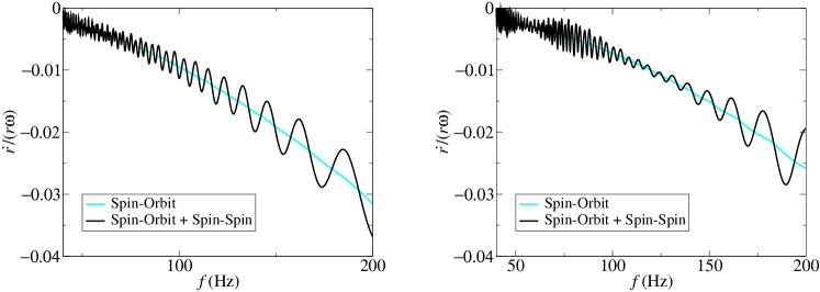
Figure 8: Oscillations in $\dot{r}$ when spin-spin interactions are present, in $(10+10)M_{\odot}$ (left panel) and $(15+5)M_{\odot}$ (right panel) binaries. Dark curves show $\dot{r}/(r\omega)$ as functions of $f_{\rm GW}$ when both spin-orbit and spin-spin interactions are take into account, while light curves show the same quantity when only spin-orbit interactions are included.

We note that our steps 1, 2, (2a, 2b, 2c), and 3 can still be applied to give initial conditions, even if the Hamiltonian contains spin-spin terms, although the orbits that follow will in general have oscillatory radius and orbital frequency, due to the non-existence of quasi-spherical orbits. In Fig. 8 we show the evolutions of $\dot{r}/(r\omega)$ with (dark curves) and without (light curves) spin-spin terms, for $(10+10)M_{\odot}$ (left panel) and $(15+5)M_{\odot}$ (right panel) binaries. We start evolution at 40 Hz, with $(\theta_{S_{1}},\phi_{S_{1}}\theta_{S_{2}},\phi_{S_{2}})=(60^{\circ},90^{\circ};60^{\circ},0^{\circ})$, and show the evolution up to 200 Hz.

V Comparison of waveforms and evaluation of overlaps

In harmonic coordinates, the gravitational wave emitted by a binary system at the leading quadrupole order, in terms of metric perturbation at a distance $D$, is

$$h_{ij}=\frac{H_{ij}}{D}\equiv\frac{2\mu}{D}\,\frac{d^{2}}{dt^{2}}(X_{i}\,X_{j})\,.$$ (78)

Using the leading-order equation of motion, $\ddot{X}_{k}=-{M\,X_{k}}/{R^{3}}$, we re-write the normalized perturbation $H_{ij}$ as:

$$H_{ij}={4\mu}\,\left(V_{i}\,V_{j}-M\frac{X_{i}\,X_{j}}{R^{3}}\right)\,.$$ (79)

Here $X_{i}$ and $V_{i}\equiv\dot{X}_{i}$ can be obtained straightforwardly by solving the Hamilton equations. Depending on the wave propagation direction and the orientation of the detector, the metric perturbation $h_{ij}$ has to be contracted with an appropriate “detection tensor” to give the actually detected waveform. For this we refer, for instance, to Sec. IIIC of Ref. pbcv1 and Sec. II of Ref. bcv2 (in particular see Eq.(15)).

Following Ref. bcv2 , the parameters in precessing binaries can be distinguished in binary local parameters $\{m_{1},m_{2},S_{1},S_{2},\theta_{\rm S1},\theta_{\rm S2},\phi_{\rm S1}-\phi_{\rm S2}\}$, binary directional parameters $\{\theta_{\rm L},\phi_{\rm L},\phi_{\rm S1}+\phi_{\rm S2}\}$ (which determine the orientation of the binary as a whole in space) and directional parameters $\{\Theta,\varphi,\theta,\phi,\psi\}$, describing the GW-propagation and the detector orientation [see Table I in Ref. bcv2 and discussion around it]. To these parameters we need to add the initial time and the initial orbital phase.

In the precessing convention introduced in Ref. bcv2 , the GW signal can be neatly written in terms of: (i) parameters depending on the observer’s location and orientation, $\{\Theta,\varphi,\theta,\phi,\psi\}$, which are time independent, initial time and initial orbital phase (henceforth denoted as extrinsic parameters) and (ii) parameters depending on the details of the dynamics, $\{m_{1},m_{2},S_{1},S_{2},\theta_{\rm S1},\theta_{\rm S2},\phi_{\rm S1}-\phi_{\rm S2}\}$ (henceforth denoted as intrinsic parameters). The GW signal does not depend on the binary directional parameters, $\{\theta_{\rm L},\phi_{\rm L},\phi_{\rm S1}+\phi_{\rm S2}\}$, since those parameters can be re-absorbed in the definition of the source frame at initial time and in the directional parameters $\{\Theta,\varphi,\theta,\phi,\psi\}$ through a rigid rotation of the detector-binary system.

The distinction between extrinsic and intrinsic parameters is due originally to Sathyaprakash and Owen Sathya ; O . Extrinsic parameters are parameters which change the signal shape in such a way that we do not actually need to lay down templates in the bank along those parameter directions, saving computational time. By contrast we need to lay down templates along the directions of the intrinsic parameters. In Refs. bcv2 ; pbcv1 , a semi-analytical method to maximize over the extrinsic parameters in precessing binaries has been proposed.

In view of the bad performances of the Taylor-expanded Hamiltonian, we a priori expect that the waveforms computed from STHTF models will be significantly different from the SEHPF ones. It remains, however, interesting to measure their difference in the data-analysis sense, i.e. to compute the overlaps between the two types of waveforms. If it happened that, after maximization over all possible parameters, the overlap between the two types of signals were very close to unity, one could still consider the Taylor models as effectual (in the sense of DIS98 ) representations of the EOB models. However, for practical reasons, we did not try to embark on a full maximization of the overlaps. For simplicity, we only tackled the maximization over the extrinsic parameters, and not on the intrinsic ones. The resulting partially maximized overlap is therefore only a lower bound of the fully maximized overlap. Still, this result can be considered as a reasonable measure of the “closeness” between the two sorts of models (especially because we do not wish to use models which would have significantly different physical parameters).

V.1 Lack of “closeness” between Taylor and Effective-One-Body models

In Tables 1 and 2 we study the closeness (in the sense just defined of overlap maximized only over the extrinsinc parameters) between STHTF(3,3.5) and SEHPF(3,3.5), as well as between STHTF(2,2) , and SEHPF(2,2.5) models.

We consider three typical binary masses $(10+10)M_{\odot}$, $(15+15)M_{\odot}$ and $(15+5)M_{\odot}$, and several initial spin orientations . We always fix the pattern functions $F_{+}=1$, $F_{\times}=0$ and GW propagation parameters $\Theta=\pi/4$ and $\varphi=0$ [for notations and definitions see Sec. IIIC of Ref. pbcv1 and Sec. II of Ref. bcv2 ]. The initial frequency is always set to $f_{\rm in}=30\,{\rm Hz}$ and the ending frequency $f_{\rm end}$ is determined by one of the criteria in Eqs. (63a)–(63d). In Tables 1 and 2 the two black holes are assumed to carry maximal and half-maximal spins, respectively. We list the ending frequency, the LSSO frequency and the BH radial separation at $t_{\rm fin}$ for the template and target, together with two types of overlaps: the overlaps maximized over the initial time and initial orbital phase only ($\rho_{\rm max,2}$), and the overlaps maximized over those parameters and $\{\Theta,\varphi,\alpha=f(\theta,\phi,\psi)\}$, as well, ($\rho_{\rm max,5}$), using the semi-analytical method suggested in Ref. pbcv1 . Table 1 and  2 also contains the non-spinning case.

As these tables show, the two types of models are not at all “close to each other”. The overlaps are indeed quite low, as low as $0.32$. The overlaps evidently increase when we maximize over five rather than two extrinsic parameters, but not dramatically, and only for binaries with high and comparable mass, with initial spins lying in the half-space opposite (with respect to the orbital plane) to the initial orbital angular momentum. In this case the dynamical evolution is shorter, since the LSSO occurs at lower frequency [see also Figs. 2, 3 ], and the differences in STHTF(3,3.5) and SEHPF(3,3.5) can be compensated by an offset in the extrinsic parameters of the template with respect to the target. Moreover, both the conservative dynamics for circular orbits and the GW flux predicted by SEHPF-approximants and STHTF-approximants, are closer in the anti-aligned case than in the aligned case, as can be see in Figs. 5 and 6.

However, when the binary mass ratio is significantly different from 1, the number of modulational cycles increases, and the differences in the two models can no longer be compensated by re-adjusting the template extrinsic parameters. When the initial spins are lying in the same half-space of the orbital angular momentum, the evolution is longer, the LSSO happens at high frequency [see also Figs. 2, 3 ], and in this case, even for high, comparable masses the differences both in the conservative and non-conservative late dymanics in the two models cannot be compensated by a bias in the template extrinsic parameters.

From Tables 2 we notice that all the above considerations apply also at 2PN order, where the differences in the conservative and non-conservative dynamics of STHTF and SEHPF approximants are even larger. We checked that these considerations do not change much when spins are smaller, say half-maximal.

Having confirmed that Taylor models cannot be considered as being effectively close to the EOB ones, we shall only use in the following the a priori better EOB models.

V.2 Negligible influence of the of the “transverse component” of the radiation reaction force.

Having in mind possible simplifications of the models, we first investigated the relevance of the second term in the R.H.S. of Eq. (62), i.e. the component of the radiation reaction force which is “transverse”, in the sense of being directed along $L$, and therefore orthogonal to the main “longitudinal term”, which is parallel to the momentum ${P}$). In Table 3 we study the influence of this transverse component of the RR force on the dynamics and the waveforms. For the binary masses $(10+10)M_{\odot}$, $(15+5)M_{\odot}$ and a few initial spin orientations, we evaluate the same quantities of Table 1, when including and not including the RR force along $L$ [see second and third term in Eq. (62)]. We give here only the overlaps maximized over five extrinsic parameters. We find that $\rho_{\rm max,5}$ is larger than $\sim 0.98$ in all cases. We therefore conclude that it would suffice to use a simplified RR force parallel to the linear momentum ${P}$ (as in the non-spinning circular case). One should, however, include, for better accuracy, in the coefficient of $P_{i}$ in Eq. (62) the spin-dependent terms.

V.3 Influence of the resummation of the “longitudinal” part of the radiation reaction

We consider here the “longitudinal” part of the radiation reaction, i.e. the first term on the R.H.S. of Eq. (62). This term is given by the flux function, which was written in Eq. (50) above as a straightforward PN-expansion. One can therefore either leave this longitudinal component in non-resummed, “Taylor” form, or choose to resum it by means of Padé approximants. In Table 4 we investigate how the choice of the flux function (Taylor-expanded or Padé-resummed) may affects the dynamics and the waveforms. Using in all cases the EOB Hamiltonian to describe the dynamics, we evaluate the overlaps between models using a Taylor flux and models using a Padé flux. [We maximize over the five extrinsic parameters of the EOB model.] We find that, when the initial spins are lying in the same half-space of the orbital angular momentum, after maximization over the five extrinsic parameters, the overlaps are reasonably large (larger than $0.84$), but still lower than unity. We obtain much higher overlaps when the initial spins are not lying in the same half-space of the orbital angular momentum. These results are consistent with Figs. 7 and Fig. 6.

If we assume that the equal-mass flux function is a smooth deformation of the test-mass limit one, since previous findings DIS98 ; BD2 ; DIS01 ; PS in the test-mass limit case pointed out the usefulness of Padé-resumming the flux function, we would conclude that Padé-resummed fluxes are better approximants of the numerically determined flux also in th equal-mass case.

V.4 Negligible influence of the quadrupole-monopole terms

Still in the spirit of trying to simplify the models to their crucial elements, Table 5 investigates how waveforms are affected by the quadrupole-monopole terms, and Table 6 studies how the evolution obtained by averaging the spin terms over a period may differ from the non-adiabatic evolution. Considering the high values of $\rho_{\rm max,5}$ we obtain in both cases, we can say that the quadrupole-monopole interaction and the adiabaticity of the spin terms, have little physical effects over the dynamics and waveforms. The differences can be compensated by re-adjusting the template extrinsic parameters.

V.5 Influence of the initial orbital phase

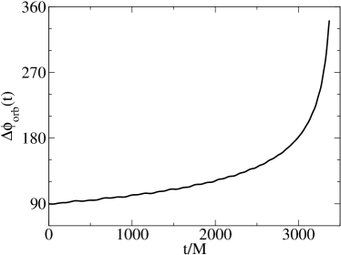
Figure 9: Relative orbital phase measured with respect to $\mathbf{S}_{\rm tot}\times\hat{\mathbf{L}}_{N}$. For maximally spinning $(15+15)M_{\odot}$ binaries, we start evolution at $40\,$Hz, with $(\theta_{S_{1}},\phi_{S_{1}};\theta_{S_{2}},\phi_{S_{2}})=(60^{\circ},90^{\circ};60^{\circ},0^{\circ})$, and orbital phases $\phi_{\rm orb}=0$ and $\pi/2$, and plot the difference $\Delta\phi_{\rm orb}$.

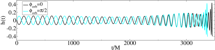
Figure 10: Comparison between waveforms from configurations with different initial orbital phases. For a $(15+15)M_{\odot}$ maximally spinning binary, we start evolution at $40\,$Hz, with $(\theta_{S_{1}},\phi_{S_{1}};\theta_{S_{2}},\phi_{S_{2}})=(60^{\circ},90^{\circ};60^{\circ},0^{\circ})$, and orbital phases $\phi_{\rm orb}=0$ and $\pi/2$, and compare the waveforms detected with $(F_{+},F_{\times};\Theta,\varphi)=(1,0;\pi/4,0)$.

Finally, we investigated the influence of the initial orbital phase (all other quantities being fixed) on the waveform. In an adiabatic evolution in which spin terms are averaged over a period the joint evolution of $\hat{\mathbf{L}}_{\rm N}$ and $\mathbf{S}$ is not affected by the initial orbital phase. As a consequence, two configurations with the same initial values for $\hat{\mathbf{L}}_{\rm N}$ and $\mathbf{S}$, but different orbital phases $\phi_{\rm orb}$ will keep the difference between orbital phases unchanged through the evolution. This may not be true in our non-adiabatic evolution for two reasons: (i) the spin-spin interaction Hamiltonian depends explicitly on the separation vector $\mathbf{N}$ [see Eq. (18)], and (ii) the evolution depends on the canonical orbital angular momentum, which is not orthogonal to the orbital plane. We illustrate this feature by evolving two maximally spinning $(15+15)M_{\odot}$ binaries with initial orbital phases (at 40 Hz) differing by $\pi/2$, and all other parameters identical: $(\theta_{S_{1}},\phi_{S_{1}};\theta_{S_{2}},\phi_{S_{2}})=(60^{\circ},90^{\circ};60^{\circ},0^{\circ})$. In Fig. 9, we plot the difference $\Delta\phi_{\rm orb}$ between their relative orbital phases measured with respect to $\hat{\mathbf{L}}_{N}$. This difference grows in time, and accumulates around $270^{\circ}$ by the end of the evolution. We also show waveforms detected with $(F_{+},F_{\times};\Theta,\varphi)=(1,0;\pi/4,0)$ in Fig. 10. Their phases start out to differ by $180^{\circ}$ as expected, and non-adiabatic effects drive them away by more than 2 cycles toward the end of the evolution. We notice that comparing the waveform is less straightforward than comparing the relative orbital phase, because the waveform phase can differ from twice the orbital phase, due to precessions.

VI Losses of energy and angular-momentum and the waveform including ringdown

In the following, we use as model the “best bet” we can make, i.e. the spinning EOB Hamiltonian with a Padé-resummed flux. Both being taken to the highest PN-accuracy available, i.e. $n=3,m=3.5$, in the notation used above.

In Ref. BD01 , using the non-spinning EOB Hamiltonian at 2PN order, it was found that the energy emitted during the plunge is $\sim 0.7\%$ of $M$, with a comparable energy loss $\sim 0.7\%$ of $M$ during the ring-down phase. This gives a total energy released beyond the LSSO in the non-spinning case of $\sim 1.4\%$ of $M$ to be contrasted with $4-5\%$ of $M$ estimated in Ref. BBCLT , where the authors use a combination of numerical and perturbative approximation methods. Note also that Flanagan and Hughes FH98 predicted $\sim 10\%M$ for inspiral and plunge, and $\sim 3\%M$ for ring-down phase.

Here, to have more confidence in our EOB-based estimates, we decided to use three different ways of evaluating the energy radiated in the spinning case. We used, at once, (i) the change, along the evolution (between some initial frequency and some final one) in the numerical value of the Hamiltonian (16) ($\delta E_{H}$), (ii) the time-integral of the square of the third derivative of the quadrupole moment $I_{ij}$ with $i,j=1,2,3$, i.e.

$$\frac{dE_{I}}{dt}=\frac{1}{5}\frac{d^{3}I_{ij}}{dt^{3}}\,\frac{d^{3}I_{ij}}{dt^{3}}\quad\quad I_{ij}=\mu\,\left(X_{i}\,X_{j}-\frac{1}{3}\delta_{ij}X^{k}\,X_{k}\right)\,.$$ (80)

and (iii) the time-integral of the energy flux carried away by our leading-order quadrupole waveform,

$$\frac{dE_{h}}{dt}=\frac{1}{20}\,\int\sum_{ij}\dot{H}_{ij}^{\rm TF}\dot{H}_{ij}^{\rm TF}\,,$$ (81)

with $H_{ij}^{\rm TF}$ being the trace-free part of the normalized metric perturbation, $H_{ij}$ [see Eq. (79) above].

In Fig. 11 we compare the accumulated energy release from these three prescriptions, for a $(15+15)M_{\odot}$ maximally spinning binary with a generic set of spin orientations when starting evolution at $f_{\rm GW}=30\,$Hz: $(\theta_{S_{1}},\phi_{S_{1}};\theta_{S_{2}},\phi_{S_{2}})=(60^{\circ},90^{\circ};60^{\circ},0^{\circ})$. In the left panel, we keep radiation reaction force at the Newtonian order, while we use 3.5PN Padé flux in the right panel. As we see from the figure, these prescriptions differ more from each other when 3.5PN radiation reaction is used instead of Newtonian — this is consistent with the fact that both $\delta E_{I}$ and $\delta E_{h}$ involve quadrupole radiation only; furthermore, for lower frequencies the $\delta E_{H}$ curve lies below those of $\delta E_{I}$ and $\delta E_{h}$, which is consistent with the fact that Post-Newtonian GW luminosity is in general smaller than the Newtonian prediction. The difference among $\delta E_{I}$ and $\delta E_{h}$ can be attributed to the difference between PN (in our case EOB at 3PN) and Newtonian dynamics, which seems to be small till around $f_{\rm GW}=200$ Hz in our case (which corresponds to $v\approx 0.45$).

The rather satisfactory agreement between the various ways of estimating the energy loss gives us some confidence in our EOB-based estimates. In the following, we shall use the a priori best estimate (because it is the one which involves the highest PN accuracy): the one based on the change in the total EOB Hamiltonian $H$. [We use Padé-resummed fluxes, and the two combined PN-accuracies $(n,m)=(2,2.5)$ and $(n,m)=(3,3.5)$.]

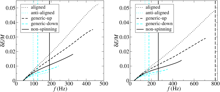
Figure 12: Accumulative energy release (upper panels) and instantaneous values of $|\mathbf{J}|/E^{2}$ (lower panels) of $(15+15)M_{\odot}$ (left panels) and $(15+5)M_{\odot}$ (right panels) binaries. LSSO frequencies for the anti-aligned, generic-down, and non-spinning configurations are shown in vertical grid lines, while LSSOs of generic-up and aligned configurations are above the ranges of our plots. [Spin-spin terms are not included in these evolutions.] We use the SEHPF(3,3.5) model.

In the upper panels of Fig. 12 we plot the accumulative energy loss $\delta E_{H}$ starting from $f_{\rm GW}=40\,$Hz as a function of the instantaneous GW frequency $f$, for $(15+15)M_{\odot}$ (upper left panel) and $(15+5)M_{\odot}$ (upper right panel) binaries, each for 4 sets of initial spin orientations with maximal spins: aligned (dash-dot-dot curves), antialigned (dotted curves), $(\theta_{S_{1}},\phi_{S_{1}};\theta_{S_{2}},\phi_{S_{2}})=(60^{\circ},90^{\circ};60^{\circ},0^{\circ})$ (denoted by generic-up, dash-dot curves), and $(\theta_{S_{1}},\phi_{S_{1}};\theta_{S_{2}},\phi_{S_{2}})=(120^{\circ},90^{\circ};120^{\circ},0^{\circ})$ (denoted by generic-down, dashed curves), as well as for the non-spinning configuration (solid curves). We use both SEHPF(3,3.5) (dark curves) and SEHPF(2,2.5) (light curves) models. In each panel, we also use vertical grid lines to mark LSSO frequencies. For the SEHPF(2,2.5) model, all our evolutions go beyond their corresponding LSSO frequencies. The situation is a bit different for the SEHPF(3,3.5). Indeed, as was shown in TD and in Fig. 3 above, the 3PN-EOB LSSO for mostly aligned fast-spinning BH’s is drastically drawn inwards towards very high orbital frequencies. So high, indeed, that, for aligned and generic-up configurations, they fall out of the frequency range plotted in Fig. 12. As a consequence, for aligned and generic-up configurations, the dynamical evolutions become rather non-adiabatic even before the formal LSSOs is reached.

As we see from the plots, within a given GW frequency interval, binaries tend to emit more energy in configurations where spins are more aligned with the orbital angular momentum. This agrees with the results of TD and of Fig. 1 above, showing that more aligned configurations are drawn towards more deeply bound states. This, together with the fact that LSSO frequencies are pushed higher in aligned configurations (as we also see from Fig. 1), can make the total energy releases in aligned configurations several times more than those in anti-aligned configurations. In Table 7, we list values of $\delta E_{H}/M$, accumulated from $40$ Hz up to LSSO frequency (if reached) or ending frequency, otherwise, for configurations plotted in Fig. 12. We also list the energy released below 40 Hz, and values of energy release when 2PN Hamiltonian and 2.5PN Padé flux are used. For $(15+15)M_{\odot}$, maximally spinning binaries, the energy released from 40 Hz up to the end of our evolution (determined by one of the criteria (63a)–(63d)) can range from $0.6\%$ of $M$ in the (anti-aligned configuration) to $5\%$ of $M$ (anti-aligned configuration), with the non-spinning configuration releasing $1.6\%\sim 1.8\%$ of $M$ (in which $0.8\%\sim 1.1\%$ of $M$ is released before LSSO). For $(15+5)M_{\odot}$ binaries, the range is similar, from $0.5\%$ to $5\%$ of $M$, with non-spinning configuration releasing $1.2\%\sim 1.4\%$ of M (in which $0.7\%\sim 0.8\%$ of M from before the LSSO). We also note that the energies of around $0.8\%$ of M and $0.5\%$ of M are released below 40 Hz, for $(15+15)M_{\odot}$ and $(15+5)M_{\odot}$ binaries, respectively. See also Eq. (4.1) of TD for an approximate analytical estimate of the energy released down to the LSSO, as a function of both $\eta=m_{1}m_{2}/M^{2}$ and $\chi_{L}$.

VI.1 Evolution of the dimensionless rotation parameter $J/E^{2}$

An important consistency check of the EOB approach concerns the dimensionless total angular momentum ratio $|\mathbf{J}|/E^{2}$ ultimately reached by spinning black hole binaries. Indeed, if the EOB method would, at the end of its validity domain, predict a ratio $|\mathbf{J}|/E^{2}$ larger than unity, this would preclude to match this end state with the newly born Kerr black hole expected from the coalescence of the two initial (spinning) black holes. This issue was investigated in the adiabatic approximation in TD . There, it was shown that, when using the 3PN-accurate EOB Hamiltonian, the ratio $|\mathbf{J}|/E^{2}$ estimated at the LSSO, was always smaller than unity. This result was not at all guaranteed in advance, and resulted from a delicate competition between the linear increase of $|\mathbf{J}|$ when increasing the (aligned) spin of the individual BH’s, and its non-linear decrease because of the displacement of the LSSO towards smaller radii for aligned spinning configurations. It was found in TD that the maximum of $(|\mathbf{J}|/E^{2})_{\rm LSSO}$ was about $0.83$, and was reached for $\chi_{L}\simeq+0.3$.

The fact that this maximum value is significantly below one, leaves room for not running into any consistency problem even when taking into account the further changes of both $E$ and ${J}$ during the plunge that follows the crossing of the LSSO. Though our present attack on the problem does not properly consider the final matching between the plunge and the formation of a final Kerr hole, it goes beyond the previous treatments in going beyond the adiabatic approximation. In the lower panels of Fig. 12, we plot the continuous time evolution of the ratio $|\mathbf{J}|/E^{2}$ during the late stages of the inspiral and its subsequent non-adiabatic ending (which, in many cases, except in fact for the most dangerous aligned, is a post-LSSO plunge). It is convenient to use the gravitational wave frequency $f_{\rm GW}$ to label the “time” along this evolution. Satisfactorily, we observe that, for all the binaries we have considered, $|\mathbf{J}|/E^{2}$ decrease to below $1$ before either the LSSO or the end of our evolution, whichever comes first. This means there are no a priori obstacles to having a Kerr black hole form right after the end of the non-adiabatic “quasi-plunge”. This means also that, contrary to an early suggestion FH98 based on rather coarse estimates, there is no ground for expecting a large emission of gravitational waves between the plunge and the merger. In Table 7 we also list the values of $|\mathbf{J}|/E^{2}$, at LSSO frequency (if reached) and ending frequency, for SEP(2,2.5) and SEP(3,3.5) models.

In a pioneering work, Baker et al. BCLT evaluated by a 3D numerical simulation the energy radiated from moderately spinning BH binaries with spins aligned or anti-aligned with the orbital angular-momentum. They started the (very short) numerical evolution close to the LSSO predicted by the effective potential method of Pfeiffer et al. PTC . As already mentioned above, the numerical initial data chosen in these works rely only on an Initial Value Problem (IVP) formulation, and significantly differ both from the numerical initial data constructed by the HKV method GGB ; Cook and from the predictions made by the EOB method (while the HKV and EOB results are quite close to each other DGG ; CookPfeiffer ). For instance, DGG estimated that the ratio between the orbital frequencies $\omega_{\rm IVP}/\omega_{\rm EOB}$ was about 2. One should probably wait until HKV-type initial data for spinning BH’s are evolved until coalescence to meaningfully compare their results with the results derived above for energy releases within the EOB approach. However, to have an idea of the current distance between analytical estimates and numerical ones, we have determined the energy released between the LSSO and the final frequency, at 2PN and 3PN order, for two of the spin configurations investigated by Baker et al. For spins aligned (anti-aligned) and $\chi_{1}=\chi_{2}=0.17$ ($\chi_{1}=\chi_{2}=0.25$), we find that the energy released is $\sim(0.6-0.9)\%M$ [$\sim(1-3)\%M$]. Baker et al. found $\sim(1.7-1.9)\%M$ and $\sim(1.9-2.1)\%M$, respectively. It should be noted that the energy released evaluated by Baker et al. includes also the ring-down phase. Ours does not.

VI.2 Complete waveforms describing the non-adiabatic inspiral and coalescence of precessing binary black holes

Finally, though we have not yet carefully studied at which stage we could meaningfully join our “quasi-plunge” evolution to the formation of a ringing BH, we have decided, to show the promise of a purely analytical EOB-base approach to follow Ref. BD2 in matching (by requiring first-order continuity of the emitted waveform) the end of our waveform (here defined by the first violation of the “adiabatic criteria” (63a)–(63b)) to a ringdown waveform generated from the lowest $l=m=2$ quasi-normal mode of a Kerr black hole. We determine the mass and spin parameters of the final hole by the energy and angular momentum of the binary at the end of our evolution:

$$M_{\rm BH}=E_{\rm fin}\,,\quad a_{\rm BH}=\left[{|\mathbf{J}|}/{E^{2}}\right]_{\rm fin}\,.$$ (82)

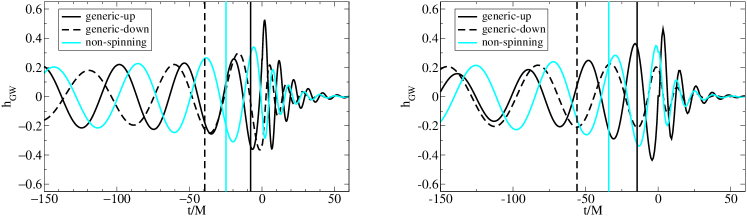
Figure 13: Inspiral waveforms (which end at $t=0$ in our plot) matched to ring-down waveforms for non-spinning (light solid curve), and half-maximally spinning $(15+15)M_{\odot}$ binaries (left panel) and $(15+5)M_{\odot}$ binaries (right panel) in the generic-up (dark solid curve) and generic-down (dark dashed curve) configurations. We start our evolutions at $40\,$Hz, and use $(F_{+},F_{\times};\Theta,\varphi)=(1,0;\pi/4,0)$. In the plot we mark the position of the LSSO with solid curves. The waveforms have been shifted in time such that the end of the inspiral occurs at $t/M=0$.

In Fig. 13, we plot the complete waveforms, so obtained, for non-spinning, and maximally spinning $(15+15)M_{\odot}$ binaries in the generic-up and generic-down configurations (these refer to the configuration at $f_{\rm GW}=40\,$Hz, the starting point of evolution). We have shifted these waveforms in time so that the end of inspiral evolutions all happen at $t=0$. Notice that at this stage the waveform which includes the ring-down phase should be considered as an example. Indeed, by restricting ourselves to the quasi-normal mode $l=m=2$, we have tacitly assumed that the total angular momentum at the time the ring-down phase starts is dominated by the orbital angular momentum. However, this is not generally the case when spins are present and the quasi-normal modes with $l\neq 2$ might be excited, as well, and contribute to the waveform. A more thourough analysis is left for the future.

VII Conclusions

We provided a first attack on the problem of analytically determining the gravitational waveforms emitted during the last stages of dynamical evolution of precessing binaries of spinning black holes, i.e. during the non-adiabatic ending of the inspiral phase, and its transition to a plunge. We reviewed the various available Hamiltonian descriptions of the dynamics of spinning black hole (BH) binaries, and studied (following TD ) the characteristics of the stable spherical orbits that exist when spin-spin effects are neglected compared to spin-orbit ones. We derived the contribution to radiation reaction (for quasi-circular orbits) which is linear in the spins. Our results agree with the corresponding recent results of Will . We then used this analytical description of the radiation-reaction-driven inspiral of spinning binaries to construct non-adiabatic models of coalescing binary waveforms. We compared the various models and concluded, in confirmation of previous results, that our current “best bet” for a non-adiabatic model describing the transition from adiabatic inspiral to plunge is obtained by combining: (i) an effective one body (EOB)  BD1 ; BD2 , 3PN-accurate DJS resummed Hamiltonian, including spin-dependent interactions TD , with (ii) Padé-resummed radiation reaction force (including spin-terms). Conclusion (i) is rather robust, since as Fig. 1 shows, the PN-expanded Hamiltonian does not show any LSSO and differs significantly from the PN-expanded analytically computed function ${E}(\Omega)$; conclusion (ii) is based on the assumption that the flux function in the equal-mass case is a smooth deformation of the test-mass limit result. Since in the latter case Padé approximants were shown DIS98 ; PS to have better agreement with exact numerical flux functions, we would conclude that this is also true in the equal-mass case.

Our main results, obtained by means of this “best bet” EOB model are:

(1) An estimate of the energy and angular momentum released by the binary system during its last stages of evolution: inspiral, transition from inspiral to plunge, and plunge;

(2) The finding (which confirms the conclusions of TD ) that the dimensionless rotation parameter $j/E^{2}$ is always smaller than unity at the end of the inspiral;

(3) The construction of complete waveforms, approximately describing the entire gravitational-wave emission process from precessing binaries of spinning black holes: adiabatic inspiral, non-adiabatic transition between inspiral and plunge, plunge, merger and ringdown. Following BD2 these waveforms were constructed by matching a quasi-normal-mode ringdown to the end of the plunge signal. These tentative complete waveforms are preliminary because we did not include here a careful study of how to join, in a physically motivated manner, the last stages of the plunge to the merger phase. They extend, however, the (better justified) complete waveforms constructed in BD2 to the more genral case of spinning and precessing binaries.

$(\theta_{\rm S1},\phi_{\rm S2},\theta_{\rm S1},\phi_{\rm S2})$	$f_{\rm fin}^{\rm SEP}$ (Hz)	$f_{\rm LSSO}^{\rm SEP}$(Hz)	${\rm R}_{\rm fin}^{\rm SEP}/M$	$f_{\rm fin}^{\rm SHT}$(Hz)	$f_{\rm LSSO}^{\rm SHT}$(Hz)	${\rm R}_{\rm fin}^{\rm SHT}/M$	$\rho_{\rm max,2}$	$\rho_{\rm max,5}$
$(10+10)M_{\odot}$
no spin	289	285	4.8	287	285	4.2	0.9150	-
$(0^{o},0^{o},0^{o},0^{o})$	745	2145	2.5	466	2145	2.8	0.3750	-
$(180^{o},0^{o},0^{o},0^{o})$	290	285	4.8	285	285	4.2	0.9166	-
$(180^{o},0^{o},180^{o},0^{o})$	145	145	8.1	145	145	7.4	0.5587	-
$(60^{o},90^{o},60^{o},0^{o})$	633	873	2.6	502	502	2.6	0.4851	0.5883
$(120^{o},90^{o},60^{o},0^{o})$	280	280	4.9	269	269	4.4	0.5420	0.9472
$(120^{o},90^{o},120^{o},0^{o})$	187	187	6.7	186	186	6.0	0.6096	0.9536
$(15+15)M_{\odot}$
no spin	192	190	4.8	192	190	4.2	0.8137	-
$(0^{o},0^{o},0^{o},0^{o})$	497	1430	2.6	311	1430	2.6	0.4550	-
$(180^{o},0^{o},0^{o},0^{o})$	193	190	4.8	191	190	4.2	0.8148	-
$(180^{o},0^{o},180^{o},0^{o})$	98	97	8.0	97	97	7.4	0.6403	-
$(60^{o},90^{o},60^{o},0^{o})$	429	758	2.6	347	347	2.4	0.5067	0.6290
$(120^{o},90^{o},60^{o},0^{o})$	185	185	4.9	180	180	4.4	0.5112	0.9456
$(120^{o},90^{o},120^{o},0^{o})$	124	124	6.7	124	124	6.7	0.6868	0.9684
$(15+5)M_{\odot}$
no spin	267	265	5.2	265	265	4.2	0.6023	-
$(0^{o},0^{o},0^{o},0^{o})$	862	1442	2.3	479	1442	2.5	0.3268	-
$(180^{o},0^{o},0^{o},0^{o})$	176	175	7.0	177	175	6.2	0.5188	-
$(180^{o},0^{0},180^{o},0^{o})$	141	140	8.3	140	140	7.5	0.4445	-
$(60^{o},90^{o},60^{o},0^{o})$	715	796	2.4	425	743	2.4	0.4478	0.6111
$(120^{o},90^{o},60^{o},0^{o})$	208	207	6.2	208	208	5.3	0.5471	0.7496
$(120^{o},90^{o},120^{o},0^{o})$	224	224	5.9	225	225	4.9	0.5735	0.8360

Table 1: We list the overlaps between STHTF(3,3.5), used as target model, and SEHPF(3,3.5), used as template model, for several binary masses and initial spin orientations. The two black holes are assumed to carry maximal spins $\chi_{1}=\chi_{2}=1$, but for comparion we also show the results in absence of spins. The evolution starts at $f_{\rm in}=30$ Hz. In the first three columns we list the ending frequency, the LSSO frequency and the BH radial separation at $t_{\rm fin}$ for the template model and in the second three columns we show the same quantities but for the target model. The last two columns contains the overlap maximized only over 2 extrinsic parameters $\rho_{\rm max,2}$ and maximed over 5 extrinsic parameters $\rho_{\rm max,5}$, as described in the text. [Notice that for the spin configuration $(60^{o},90^{o},60^{o},0^{o})$ and masses $(10+10)M_{\odot}$ and $(15+5)M_{\odot}$, due to a pole in the Padé-approximant flux, we apply the Padé resummation only to the non-spinning terms in the flux.]

$(\theta_{\rm S1},\phi_{\rm S2},\theta_{\rm S1},\phi_{\rm S2})$	$f_{\rm fin}^{\rm SEP}$ (Hz)	$f_{\rm LSSO}^{\rm SEP}$(Hz)	${\rm R}_{\rm fin}^{\rm SEP}/M$	$f_{\rm fin}^{\rm SHT}$(Hz)	$f_{\rm LSSO}^{\rm SHT}$(Hz)	${\rm R}_{\rm fin}^{\rm SHT}/M$	$\rho_{\rm max,2}$	$\rho_{\rm max,5}$
$(10+10)M_{\odot}$
no spin	242	237	5.6	237	237	4.5	0.4691	-
$(0^{o},0^{o},0^{o},0^{o})$	628	628	2.9	628	628	2.6	0.3170	-
$(180^{o},0^{o},0^{o},0^{o})$	237	237	5.6	237	237	4.5	0.4681	-
$(180^{o},0^{o},180^{o},0^{o})$	139	139	8.4	139	139	7.6	0.6433	-
$(60^{o},90^{o},60^{o},0^{o})$	367	367	4.1	342	342	3.5	0.4197	0.4882
$(120^{o},90^{o},60^{o},0^{o})$	234	234	5.7	229	229	4.7	0.4220	0.6015
$(120^{o},90^{o},120^{o},0^{o})$	173	173	7.1	172	172	6.3	0.6681	0.9556
$(15+15)M_{\odot}$
no spin	158	158	5.6	158	158	4.5	0.4880	-
$(0^{o},0^{o},0^{o},0^{o})$	419	419	2.9	419	419	2.6	0.4044	-
$(180^{o},0^{o},0^{o},0^{o})$	158	158	5.6	158	158	4.5	0.4885	-
$(180^{o},0^{o},180^{o},0^{o})$	93	93	8.4	93	93	7.6	0.7140	-
$(60^{o},90^{o},60^{o},0^{o})$	240	238	4.2	241	241	4.1	0.4549	0.5186
$(120^{o},90^{o},60^{o},0^{o})$	156	155	5.7	152	152	4.7	0.4827	0.6767
$(120^{o},90^{o},120^{o},0^{o})$	115	115	7.1	116	116	6.2	0.7227	0.9442
$(15+5)M_{\odot}$
no spin	232	232	5.7	233	232	4.7	0.6111	-
$(0^{o},0^{o},0^{o},0^{o})$	608	608	2.9	608	608	2.6	0.2695	-
$(180^{o},0^{o},0^{o},0^{o})$	167	166	7.3	166	166	6.5	0.8720	-
$(180^{o},0^{0},180^{o},0^{o})$	136	136	8.5	136	136	7.7	0.6743	-
$(60^{o},90^{o},60^{o},0^{o})$	352	352	4.2	367	367	3.2	0.2696	0.4978
$(120^{o},90^{o},60^{o},0^{o})$	192	192	6.6	191	191	5.7	0.6566	0.8173
$(120^{o},90^{o},120^{o},0^{o})$	169	169	7.2	167	167	6.5	0.6207	0.8970

Table 2: Overlaps between STHTF(2,2), used as target model, and SEHPF(2,2.5), used as template model, for several binary masses and initial spin orientations. The two black holes are assumed to carry maximal spins $\chi_{1}=\chi_{2}=1$, but for comparion we also show the results in absence of spins. The evolution starts at $f_{\rm in}=30$ Hz. In the first three columns we list the ending frequency, the LSSO frequency and the BH radial separation at $t_{\rm fin}$ for the template model and in the second three columns we show the same quantities but for the target model. The last two columns contains the overlap maximized only over 2 extrinsic parameters $\rho_{\rm max,2}$ and maximed over 5 extrinsic parameters $\rho_{\rm max,5}$, as described in the text.

$(\theta_{\rm S1},\phi_{\rm S2},\theta_{\rm S1},\phi_{\rm S2})$	$f_{\rm fin}^{\rm SEP,noF_{L}}$ (Hz)	$f_{\rm LSSO}^{\rm SEP,noF_{L}}$ (Hz)	${\rm R}_{\rm fin}^{\rm SEP,noF_{L}}/M$	$f_{\rm fin}^{\rm SEP}$(Hz)	$f_{\rm LSSO}^{\rm SEP}$ (Hz)	${\rm R}_{\rm fin}^{\rm SEP}/M$	$\rho_{\rm max,5}$
$(10+10)M_{\odot}$
$(60^{o},90^{o},60^{o},0^{o})$	633	872	2.7	660	1211	2.7	0.9860
$(120^{o},90^{o},120^{o},0^{o})$	187	186	6.7	186	186	6.7	0.9953
$(15+5)M_{\odot}$
$(60^{o},90^{o},60^{o},0^{o})$	743	767	2.3	564	564	2.9	0.9839
$(120^{o},90^{o},120^{o},0^{o})$	178	177	7.0	179	179	6.9	0.9969

Table 3: Effect of radiation-reaction force along $L$ over the binary evolution and waveforms by comparing SEHPF(3,3.5) with no $F_{L}$, used as target model, and SEHPF(3,3.5), used as template model, for several binary masses and initial spin orientations. The two black holes are assumed to carry maximal spins $\chi_{1}=\chi_{2}=1$. The evolution starts at $f_{\rm in}=30$ Hz. In the first three columns we list the ending frequency, the LSSO frequency and the BH radial separation at $t_{\rm fin}$ for the template model and in the second three columns we show the same quantities but for the target model. The last two columns contains the overlap maximized only over 2 extrinsic parameters $\rho_{\rm max,2}$ and maximed over 5 extrinsic parameters $\rho_{\rm max,5}$, as described in the text. [Notice that for the spin configuration $(60^{o},90^{o},60^{o},0^{o})$ and masses $(10+10)M_{\odot}$ and $(15+5)M_{\odot}$, due to a pole in the Padé-approximant flux, we apply the Padé resummation only to the non-spinning terms in the flux.]

$(\theta_{\rm S1},\phi_{\rm S2},\theta_{\rm S1},\phi_{\rm S2})$	$f_{\rm fin}^{\rm SET}$ (Hz)	$f_{\rm LSSO}^{\rm SET}$(Hz)	${\rm R}_{\rm fin}^{\rm SET}/M$	$f_{\rm fin}^{\rm SEP}$(Hz)	$f_{\rm LSSO}^{\rm SEP}$(Hz)	${\rm R}_{\rm fin}^{\rm SEP}/M$	$\rho_{\rm max,5}$
$(10+10)M_{\odot}$
$(60^{o},90^{o},60^{o},0^{o})$	632	872	2.6	616	1252	2.6	0.8566
$(120^{o},90^{o},120^{o},0^{o})$	185	185	6.7	186	185	6.7	0.9762
$(15+5)M_{\odot}$
$(60^{o},90^{o},60^{o},0^{o})$	743	767	2.3	661	772	2.5	0.8232
$(120^{o},90^{o},120^{o},0^{o})$	178	177	7.0	179	178	6.9	0.9913

Table 4: Effect of Padé and Taylor flux on the binary evolution and waveforms by comparing SEHTF(3,3.5), used as target model, and SEHPF(3,3.5), used as template model, for several binary masses and initial spin orientations. The two black holes are assumed to carry maximal spins $\chi_{1}=\chi_{2}=1$. The evolution starts at $f_{\rm in}=30$ Hz. In the first three columns we list the ending frequency, the LSSO frequency and the BH radial separation at $t_{\rm fin}$ for the template model and in the second three columns we show the same quantities but for the target model. The last two columns contains the overlap maximized only over 2 extrinsic parameters $\rho_{\rm max,2}$ and maximed over 5 extrinsic parameters $\rho_{\rm max,5}$, as described in the text. [Notice that for the spin configuration $(60^{o},90^{o},60^{o},0^{o})$ and masses $(10+10)M_{\odot}$ and $(15+5)M_{\odot}$, due to a pole in the Padé-approximant flux, we apply the Padé resummation only to the non-spinning terms in the flux.]

$(\theta_{\rm S1},\phi_{\rm S2},\theta_{\rm S1},\phi_{\rm S2})$	$f_{\rm fin}^{\rm SEP,noQM}$ (Hz)	$f_{\rm LSSO}^{\rm SEP,noQM}$(Hz)	${\rm R}_{\rm fin}^{\rm SEP,noQM}/M$	$f_{\rm fin}^{\rm SEP}$(Hz)	$f_{\rm LSSO}^{\rm SEP}$(Hz)	${\rm R}_{\rm fin}^{\rm SEP}/M$	$\rho_{\rm max,5}$
$(10+10)M_{\odot}$
$(60^{o},90^{o},60^{o},0^{o})$	650	1257	2.6	633	872	2.6	0.9959
$(120^{o},90^{o},60^{o},0^{o})$	185	184	6.8	186	186	6.7	0.9988
$(15+5)M_{\odot}$
$(60^{o},90^{o},60^{o},0^{o})$	702	766	2.3	743	767	2.3	0.9823
$(120^{o},90^{o},120^{o},0^{o})$	178	178	7.0	178	177	7.0	0.9979

Table 5: Effect of quadrupole-monopole (QM) interaction on the binary evolution and waveforms by comparing SEHPF(3,3.5) with QM interaction, used as target model, and SEHPF(3,3.5) without QM terms, used as template model, for several binary masses and initial spin orientations. The two black holes are assumed to carry maximal spins $\chi_{1}=\chi_{2}=1$. The evolution starts at $f_{\rm in}=30$ Hz. In the first three columns we list the ending frequency, the LSSO frequency and the BH radial separation at $t_{\rm fin}$ for the template model and in the second three columns we show the same quantities but for the target model. The last two columns contains the overlap maximized only over 2 extrinsic parameters $\rho_{\rm max,2}$ and maximed over 5 extrinsic parameters $\rho_{\rm max,5}$, as described in the text. [Notice that for the spin configuration $(60^{o},90^{o},60^{o},0^{o})$ and masses $(10+10)M_{\odot}$ and $(15+5)M_{\odot}$, due to a pole in the Padé-approximant flux, we apply the Padé resummation only to the non-spinning terms in the flux.]

$(\theta_{\rm S1},\phi_{\rm S2},\theta_{\rm S1},\phi_{\rm S2})$	$f_{\rm fin}^{\rm SEP,adiab}$ (Hz)	$f_{\rm LSSO}^{\rm SEP,adiab}$(Hz)	${\rm R}_{\rm fin}^{\rm SEP,adiab}/M$	$f_{\rm fin}^{\rm SEP}$(Hz)	$f_{\rm LSSO}^{\rm SEP}$(Hz)	${\rm R}_{\rm fin}^{\rm SEP}/M$	$\rho_{\rm max,5}$
$(10+10)M_{\odot}$
$(60^{o},90^{o},60^{o},0^{o})$	636	1185	2.6	633	872	2.7	0.9666
$(120^{o},90^{o},120^{o},0^{o})$	186	185	6.7	186	186	6.7	0.9932
$(15+5)M_{\odot}$
$(60^{o},90^{o},60^{o},0^{o})$	699	827	2.3	743	767	2.3	0.9665
$(120^{o},90^{o},120^{o},0^{o})$	177	177	7.0	178	177	7.0	0.9914

Table 6: Effect of assuming that spins evolve adiabatically. We compare SEHPF(3,3.5), used as target model, and SEHPF(3,3.5) obtained by averaging the spin couplings over an orbit, as template model, for several binary masses and initial spin orientations. The two black holes are assumed to carry maximal spins $\chi_{1}=\chi_{2}=1$. The evolution starts at $f_{\rm in}=30$ Hz. In the first three columns we list the ending frequency, the LSSO frequency and the BH radial separation at $t_{\rm fin}$ for the template model and in the second three columns we show the same quantities but for the target model. The last two columns contains the overlap maximized only over 2 extrinsic parameters $\rho_{\rm max,2}$ and maximed over 5 extrinsic parameters $\rho_{\rm max,5}$, as described in the text. [Notice that for the spin configuration $(60^{o},90^{o},60^{o},0^{o})$ and masses $(10+10)M_{\odot}$ and $(15+5)M_{\odot}$, due to a pole in the Padé-approximant flux, we apply the Padé resummation only to the non-spinning terms in the flux.]

$(\theta_{\rm S1},\phi_{\rm S1},\theta_{\rm S2},\phi_{\rm S2})$	$[\delta E_{H}]_{f<40\,{\rm Hz}}/M$	$f_{\rm LSSO}$ (Hz)	$[\delta E_{H}]_{\rm LSSO}^{40\,{\rm Hz}}/M$	$\left[|\mathbf{J}|/E^{2}\right]_{\rm LSSO}$	$f_{\rm fin}$	$\left[\delta E_{H}\right]_{\rm fin}^{40,{\rm Hz}}/M$	$\left[|\mathbf{J}|/E^{2}\right]_{\rm fin}$
$(15+15)M_{\odot}$, 3PN
nospin	0.0082	190	0.0107	0.82	325	0.0182	0.77
($0^{\circ}$,$0^{\circ}$,$0^{\circ}$,$0^{\circ}$)	0.0086	(1430)	$-$	$-$	474	0.0527	0.96
($180^{\circ}$,$0^{\circ}$,$180^{\circ}$,$0^{\circ}$)	0.0077	97	0.0033	0.51	194	0.0064	0.47
($60^{\circ}$,$90^{\circ}$,$60^{\circ}$,$0^{\circ}$)	0.0084	(760)	$-$	$-$	440	0.0352	0.91
($120^{\circ}$,$90^{\circ}$,$120^{\circ}$,$0^{\circ}$)	0.0079	123	0.0054	0.74	242	0.0101	0.70
$(15+5)M_{\odot}$, 3PN
nospin	0.0048	265	0.0084	0.62	484	0.0141	0.58
($0^{\circ}$,$0^{\circ}$,$0^{\circ}$,$0^{\circ}$)	0.0049	(1442)	$-$	$-$	819	0.0493	0.95
($180^{\circ}$,$0^{\circ}$,$180^{\circ}$,$0^{\circ}$)	0.0046	140	0.0034	0.14	289	0.0054	0.11
($60^{\circ}$,$90^{\circ}$,$60^{\circ}$,$0^{\circ}$)	0.0049	(793)	$-$	$-$	719	0.0294	0.91
($120^{\circ}$,$90^{\circ}$,$120^{\circ}$,$0^{\circ}$)	0.0047	177	0.0049	0.62	351	0.0080	0.60

Table 7: Energy released and the magnitude of angular momentum through the evolution (with spin-spin terms ignored). For non-spinning binaries, and four configurations of maximally spinning binaries, we give the energy released below 40 Hz, from 40 Hz up to the LSSO, and from 40 Hz up to to the end of the evolution. [In some cases the evolution stops before LSSO can be reached.] We also show the corresponding values of $|\mathbf{J}|/E^{2}$. Note that these results do not include the ring-down phase.

Figure 11: Comparison between the three different prescriptions, $\delta E_{I}$ (dashed curves), $\delta E_{h}$ (dotted curves) and $\delta E_{H}$ (solid curves), for calculating energy losses. We use Newtonian-order radiation reaction in the left panel, and Padé at 3.5PN order in the right panel. We use the EOB Hamiltonian at 3PN order