Neutron Stars – Cooling and Transport

Abstract

Observations of thermal radiation from neutron stars can potentially provide information about the states of supranuclear matter in the interiors of these stars with the aid of the theory of neutron-star thermal evolution. We review the basics of this theory for isolated neutron stars with strong magnetic fields, including most relevant thermodynamic and kinetic properties in the stellar core, crust, and blanketing envelopes.

1 Introduction

The first works on neutron star cooling and thermal emission (Stabler 1960; Tsuruta 1964; Chiu and Salpeter 1964; Morton 1964; Bahcall and Wolf 1965a, b) appeared at the epoch of the discoveries of X-ray sources outside the Solar System in the rocket and balloon experiments (Giacconi et al. 1962; Bowyer et al. 1964a, b). The authors estimated cooling rates and surface temperatures in order to answer the question, whether a neutron star can be detected in this kind of experiments. However, the first attempts failed to prove the relation between neutron stars and newly discovered X-ray sources. In particular, Bowyer et al. (1964b) measured the size of the X-ray source in the Crab Nebula from observations during a lunar occultation on July 7, 1964. Their result, $\sim 10^{13}$ km, indicated that the source was much larger than a neutron star should be. Ironically, there was a neutron star there, the famous Crab pulsar, but it was hidden within a compact plerion pulsar nebula. Kardashev (1964) and later Pacini (1967) conjectured that the Crab Nebula could be powered by the neutron-star rotational energy, which was transferred to the nebula via the magnetic field, but this model remained a hypothesis. Curiously, the Crab pulsar was observed as a scintillating radio source since 1962 (Hewish and Okoye 1965), but the nature of this source remained unclear. Sandage et al. (1966) identified Sco X-1, the first detected and the brightest cosmic X-ray source, as an optical object of 13th magnitude. Shklovsky (1967) analyzed these observations and concluded that the X-ray radiation of Sco X-1 originated from the accretion of matter onto a neutron star from its companion. Later this conjecture was proved to be true (de Freitas Pacheco et al. 1977), but at the time it was refuted (Cameron 1967). Because of these early confusions, the first generally accepted evidence of neutron stars was provided only by the discovery of pulsars (Hewish et al. 1968) after a successful competition of the theoretical interpretation of pulsars as rotating neutron stars (Gold 1968) with numerous alternative hypotheses (see, e.g., the review by Ginzburg 1971).

The foundation of the rigorous cooling theory was laid by Tsuruta (1964) and Tsuruta and Cameron (1966), who formulated the main elements of the theory: the relation between the internal and surface temperatures of a neutron star, the neutrino and photon cooling stages, etc. After the discovery of neutron stars, a search for their soft X-ray thermal emission has become a topical challenge, which stimulated the development of the cooling theory. The first decade of this development was reviewed by Tsuruta (1979) and Nomoto and Tsuruta (1981a).

Thorne (1977) presented the complete set of equations describing the mechanical and thermal structure and evolution of a spherically symmetric star at hydrostatic equilibrium in the framework of General Relativity (GR). The GR effects on the thermal evolution of neutron stars were first included into the cooling calculations by Glen and Sutherland (1980); Nomoto and Tsuruta (1981b); Van Riper and Lamb (1981). A generally relativistic cooling code for a spherically symmetric non-barotropic star was written by Richarson et al. (1982). Nomoto and Tsuruta (1986, 1987) studied neutron star cooling using an updated physics input and discussed the role of different physical factors for thermal relaxation of different models of neutron stars. Tsuruta (1986) provided a comprehensive review of the neutron star cooling theory with a comparison of the results of different research groups obtained by mid-1980s.

The early studies of the neutron-star cooling were mostly focused on the standard scenario where the neutrino emission from the stellar core was produced mainly by the modified Urca (Murca) processes, which compete with neutrino emission via plasmon decay, nucleon bremsstrahlung, etc. The enhanced (accelerated) cooling due to the direct Urca (Durca) processes was believed possible only if the core contains a pion condensate or a quark plasma (e.g., Tsuruta 1979; Glen and Sutherland 1980; Van Riper and Lamb 1981; Richarson et al. 1982). By the end of 1980s a new cooling agent, kaon condensate, was introduced (Brown et al. 1988; Page and Baron 1990). The studies of the enhanced cooling were intensified after the discovery by Lattimer et al. (1991) that the Durca process is allowed in the neutron star core with the standard nuclear composition for some realistic equations of state (EoS) without “exotic” models. The standard and Durca-enhanced neutron star cooling scenarios were compared in a number of numerical simulations starting from Page and Applegate (1992), who also noticed that nucleon superfluidity becomes the strongest cooling regulator in the Durca-allowed stellar kernels. This result triggered a flow of papers on the cooling of superfluid neutron stars.

The progress in the theoretical studies of the neutron-star thermal evolution was influenced in the 1980s and 1990s by the spectacular progress of the X-ray astronomy, notably due to the space observatories Einstein (1978–1981), EXOSAT (1983–1986), and ROSAT (1990–1998). ROSAT was the first to reliably detect X-ray thermal radiation from isolated neutron stars. This theoretical and observational progress was reviewed by Tsuruta (1998); Yakovlev and Pethick (2004); Page et al. (2004).

In the 21st century, the data collected by X-ray observatories Chandra and XMM-Newton give a new impetus to the development of the cooling theory. Some new theoretical results on the cooling of neutron stars and relation of the theory to observations were reviewed by Yakovlev et al. (2008); Page (2009); Tsuruta (2009). Recently, 2D simulations of the fully coupled thermal and magnetic field evolution have been possible (Pons et al. 2009; Viganò et al. 2013), mostly motivated by the increasing number of observed magnetars and high magnetic field pulsars.

The theory of thermal evolution of neutron stars has different aspects associated with rotation, accretion, etc. In this review, we will mostly focus on the physics that determines thermal structure and evolution of slowly rotating non-accreting neutron stars, whose thermal emission can be substantially affected by strong magnetic fields. The processes of formation of thermal spectra in the outermost layers of such stars are explicitly excluded from this paper but considered in the companion review (Potekhin, De Luca, and Pons 2015, hereafter Paper I). We will pay a special attention to the effects of strong magnetic fields on the thermal structure and heat conduction in the crust and heat-blanketing envelopes of neutron stars.

2 The essential physics of neutron star cooling

In this section we briefly present the essential physical ingredients needed to build a model of a cooling neutron star regardless its magnetic field. The effects of strong magnetic fields will be discussed in subsequent sections, starting from Sect. 4.

2.1 Structure and composition of a neutron star

A neutron star is born hot ($\approx 10^{11}$ K) and lepton-rich, but only a few days after its birth, its temperature drops to a few $\times 10^{9}$ K. Thus, the Fermi energy $\epsilon_{\mathrm{F}}$ of all particles is much higher than the kinetic thermal energy in most of the star volume, except in the thin outermost layers (a few meters thick), which does not affect the mechanical and thermal structure of the rest of the star. Therefore, a good approximation is to describe the state of matter as cold nuclear matter in beta equilibrium, resulting in an effectively barotropic EoS. The mechanical structure of the star is decoupled from its thermal structure and can be calculated only once and kept fixed during the thermal evolution simulations.

To a very good approximation, the mechanical structure can be assumed to be spherical. Appreciable deviations from the spherical symmetry can be caused by ultra-strong magnetic fields ($B\gtrsim 10^{17}$ G) or by rotation with ultra-short periods (less than a few milliseconds), but we will not consider such extreme cases. Then the space-time is described by the Schwarzschild metric (e.g. Misner et al. 1973)

$$\mathrm{d}s^{2}=-\mathrm{e}^{2\Phi(r)}c^{2}\mathrm{d}t^{2}+\mathrm{e}^{2\Lambda(r)}\mathrm{d}r^{2}+r^{2}(\mathrm{d}\theta^{2}+\sin^{2}\theta\mathrm{d}\varphi^{2}),$$ (1)

where $(r,\theta,\varphi)$ are the standard spherical coordinates, $\mathrm{e}^{2\Lambda(r)}=1-2GM_{r}/c^{2}r$, and $\Phi(r)$ is determined by equation

$$\mathrm{d}\Phi(r)/\mathrm{d}P(r)=-\big{[}P(r)+\rho(r)c^{2}\big{]}^{-1}$$ (2)

with the boundary condition $\mathrm{e}^{2\Phi(R)}=1-r_{g}/R$ at the stellar radius $R$. Here, $r_{g}=2GM/c^{2}=2.95(M/M_{\odot})$ km is the Schwarzschild radius, $M\equiv M_{R}$ is the stellar mass, $M_{r}=4\pi\int_{0}^{r}\rho(r)r^{2}\mathrm{d}r$ is the mass inside a sphere of radius $r$, $G$ is the gravitational constant, $c$ is the speed of light, $P$ is the pressure, and $\rho$ is the gravitational mass density.

The mechanical structure of a spherically symmetric star is described by the Tolman-Oppenheimer-Volkoff equation

$$\frac{\mathrm{d}P}{\mathrm{d}r}=-\frac{GM_{r}\,\rho}{r^{2}}\,\left(1+\frac{P}{\rho c^{2}}\right)\,\left(1+\frac{4\pi r^{3}P}{M_{r}c^{2}}\right)\,\left(1-\frac{2GM_{r}}{rc^{2}}\right)^{-1},$$ (3)

where $r$ is the radial coordinate measured from the stellar center. In order to determine the stellar mechanical structure, Eq. (3) should be supplemented by an EoS, which depends on a microscopic physical model (Sect. 2.4). Several qualitatively different regions can be distinguished in a neutron star, from the center to the surface: the inner and outer core, the mantle, the inner and outer crust, the ocean, and the atmosphere (e.g., Haensel et al. 2007).

The outer core of a neutron star has mass density $0.5\rho_{0}\lesssim\rho\lesssim 2\rho_{0}$, where $\rho_{0}=2.8\times 10^{14}$ g cm^-3 is the nuclear saturation density (the typical density of a heavy atomic nucleus). It is usually several kilometers thick and contains most of the stellar mass. The outer core is mostly composed of neutrons with an admixture of the protons and leptons – electrons and muons ($npe\mu$ matter).

The inner core, which can exist in rather massive neutron stars, $M\gtrsim 1.5\,M_{\odot}$, occupies the central part with $\rho\gtrsim 2\rho_{0}$. It is defined as the region where the composition is uncertain, but probably more rich than simply neutrons and protons. Its composition and properties are not well known because the results of their calculation strongly depend on details on the theoretical model of collective fundamental interactions. Some of the proposed models envision the following hypothetical options:

• hyperonization of matter – the appearance of various hyperons (first of all, $\Lambda$- and $\Sigma^{-}$-hyperons – $npe\mu\Lambda\Sigma$ matter);

• pion condensation – formation of a Bose condensate of collective interactions with the properties of $\pi$-mesons;

• kaon condensation – formation of a similar condensate of $K$-mesons;

• deconfinement – phase transition to quark matter.

The last three options are often called exotic (Haensel et al. 2007, Chapt. 7). In this paper we will not consider the exotic matter in any detail.

In the stellar crust and ocean the matter is less extraordinary: it contains electrons, nuclei composed of protons and neutrons, and, in the inner crust, quasi-free neutrons. Nevertheless, this region is also under extreme conditions (density, temperature, magnetic field) that cannot be reproduced in the laboratory. In the crust, which is normally $\sim 1$ km thick, the nuclei are arranged into a crystalline lattice, and in the ocean with a typical depth from a few to $\sim 100$ meters (depending on temperature) they form a liquid (see Sect. 2.4.1).

With increasing density, nuclei become progressively neutron-rich due to the beta-captures that are favored by the increase of pressure of the degenerate electrons. Neutrons start to drip out of nuclei at density $\rho_{\mathrm{drip}}=4.3\times 10^{11}$ g cm^-3. Thus at $\rho>\rho_{\mathrm{drip}}$ neutron-rich nuclei are embedded in the sea of quasi-free neutrons.

At the bottom of the crust, the nuclei may take rodlike and platelike shapes to compose so called pasta phases of nuclear matter (Pethick and Ravenhall 1995). Then they form a mantle with anisotropic kinetic properties (Pethick and Potekhin 1998). Thermodynamic stability of the pasta phase state and, therefore, the existence of the mantle depends on the model of nuclear interactions. Lorenz et al. (1993) demonstrated stability of the pasta phases at $\rho\gtrsim 10^{14}$ g cm^-3 for the FPS EoS model of Pandharipande and Ravenhall (1989), but they were not found to be stable in modern EoS models SLy (Douchin and Haensel 2001) and BSk (Pearson et al. 2012).

The strong gravity drives the rapid separation of chemical elements in the crust and the ocean. Estimates of characteristic sedimentation time range from seconds to months, depending on local conditions and composition (see, e.g., Eq. 20 in Potekhin 2014), which is a very short timescale compared to the stellar age. Therefore the envelopes are thought to be made of chemically pure layers, which are separated by narrow transition bands of diffusive mixing (De Blasio 2000; Chang et al. 2010).

2.2 Thermal evolution equations

The multidimensional heat transport and thermal evolution equations in a locally flat reference frame read (e.g., Aguilera et al. 2008; Pons et al. 2009; Viganò et al. 2013)

$$c_{\mathrm{v}}\,\mathrm{e}^{\Phi}\,\frac{\partial T}{\partial t}+\nabla\cdot(\mathrm{e}^{2\Phi}\bm{F})=\mathrm{e}^{2\Phi}(H-Q_{\nu}),\qquad\bm{F}=-\mathrm{e}^{-\Phi}\hat{\kappa}\cdot\nabla(\mathrm{e}^{\Phi}T),$$ (4)

where $\bm{F}$ is the heat flux density, $H$ is the heating power per unit volume, $c_{\mathrm{v}}$ is specific heat (Sects. 2.5, 3.2, and 4.2), $Q_{\nu}$ is neutrino emissivity (Sects. 2.6, 3.3, 4.3), $\hat{\kappa}$ is the thermal conductivity tensor (Sects. 2.7, 3.4, and 4.4), and $\nabla=(\mathrm{e}^{-\Lambda(r)}\partial/\partial r,\,r^{-1}\partial/\partial\theta,\,(r\sin\theta)^{-1}\partial/\partial\varphi)$ in compliance with Eq. (1). The inner boundary condition to the system of equations (4) is $\bm{F}=0$ at $r=0$. The outer boundary condition is determined by the properties of a heat-blanketing envelope, which serves as a mediator of the internal heat into the outgoing thermal radiation. It will be considered in Sect. 5. Solutions to the thermal evolution equations and their implications are briefly reviewed in Sect. 6.

For weak magnetic fields, we can assume that the temperature gradients are essentially radial, and that in most of the star volume (inner crust and core) the conductivity tensor is simply a scalar quantity times the identity matrix. In this limit, corrections for deviations from the 1D approximation have little effect on the total luminosity. However, for strong fields and neutron stars with locally intense internal heating sources, such as magnetars, a more accurate description, beyond the 1D approximation, must be considered.

2D calculations of thermal structure and evolution of strongly magnetized neutron stars have been done by several groups (Geppert et al. 2004, 2006; Pérez-Azorin et al. 2006; Aguilera et al. 2008; Kaminker et al. 2012, 2014). In some of these works (Geppert et al. 2006; Pérez-Azorin et al. 2006; Aguilera et al. 2008), neutron-star models with superstrong ($B\sim 10^{15}$ – $10^{16}$ G) toroidal magnetic fields in the crust were considered, in addition to the less strong ($B\sim 10^{12}$ – $10^{14}$ G) poloidal component that penetrates from the crust into the magnetosphere. The latter models help to explain the strongly non-uniform distribution of the effective temperature over the neutron-star surface and the possible energy source for magnetars outbursts (Pons and Perna 2011; Pons and Rea 2012). Only recently (Viganò et al. 2013), the fully coupled evolution of temperature and magnetic field has been studied with detailed numerical simulations, which allow one to follow the long-term evolution of magnetars and their connection with other neutron star classes. Some results of such calculations will be discussed in Sect. 6.

2.3 Basic plasma parameters

In this section we introduce several basic parameters of Coulomb plasmas that are used below. To be concrete, we start with electrons and ions (including bare atomic nuclei). When other charged particles are present, their respective parameters are defined analogously, with the obvious replacements of particle mass, charge, number density, etc.

Since the major constituents of the neutron-star matter are mostly degenerate, an important parameter is the Fermi energy, which (without the rest energy) equals

$$\epsilon_{\mathrm{F}}=c\,\sqrt{(mc)^{2}+(p_{\mathrm{F}})^{2}}-mc^{2},$$ (5)

where $m$ is the particle mass, and $p_{\mathrm{F}}$ is the Fermi momentum. For instance, for the Fermi gas in the absence of a quantizing magnetic field, $p_{\mathrm{F}}=\hbar\,(3\pi^{2}n)^{1/3}$, where $n$ is the number density, and $\hbar$ is the reduced Planck constant. It is convenient to use the dimensionless density parameter related to the Fermi momentum of electrons, $x_{\mathrm{r}}=p_{\mathrm{F}e}/m_{e}c$, where $m_{e}$ is the electron mass. In the outer core and the envelopes, as long as the baryons are non-relativistic, $x_{\mathrm{r}}\approx(\rho_{6}\,Y_{e})^{1/3}$, where $Y_{e}$ is the number of electrons per baryon and $\rho_{6}\equiv\rho/10^{6}$ g cm^-3.

Thermal de Broglie wavelengths of free ions and electrons are usually defined as $\lambda_{\mathrm{i}}=\sqrt{2\pi\hbar^{2}/m_{\mathrm{i}}T}$ and $\lambda_{e}=\sqrt{2\pi\hbar^{2}/m_{e}T},$ where $m_{\mathrm{i}}=Am_{\mathrm{u}}$ is the ion mass, and $m_{\mathrm{u}}$ is the unified atomic mass unit. Here and hereafter, we use $T$ in energy units and suppress the Boltzmann constant (i.e., $10^{6}\mbox{ K}=86.17$ eV). The quantum effects on ion motion are important either at $\lambda_{\mathrm{i}}\gtrsim a_{\mathrm{i}}$ or at $T\ll T_{\mathrm{p}}$, where $T_{\mathrm{p}}=\hbar\omega_{\mathrm{p}}$ is the ion plasma temperature, and $\omega_{\mathrm{p}}=\left({4\pi e^{2}\,n_{\mathrm{i}}}\,Z^{2}/m_{\mathrm{i}}\right)^{1/2}$ is the ion plasma frequency. Debye temperature of a crystal $\Theta_{\mathrm{D}}$ is closely related to the plasma temperature. In the harmonic approximation for the Coulomb crystal, $\Theta_{\mathrm{D}}\approx 0.45\,T_{\mathrm{p}}$ (Carr 1961).

The Coulomb plasmas are called strongly coupled if the parameter $\Gamma_{\mathrm{C}}=(Ze)^{2}/a_{\mathrm{i}}T$, which estimates the electrostatic to thermal energy ratio, is large. Here, $a_{\mathrm{i}}\equiv(\frac{4}{3}\pi n_{\mathrm{i}})^{-1/3}$ is the ion sphere, or Wigner-Seitz cell, radius, and $n_{\mathrm{i}}$ is the ion number density. If the plasma only consists of electrons and non-relativistic ions of one kind, which is typical for neutron-star envelopes, then

$$T_{\mathrm{p}}=7.832\,(Z/A)\sqrt{\rho_{6}}\times 10^{6}\mbox{~{}K},\qquad\Gamma_{\mathrm{C}}=22.747\,Z^{5/3}(\rho Y_{e})^{1/3}/T_{6}.$$ (6)

Analogously, $T_{\mathrm{p},e}=\hbar\,(4\pi e^{2}n_{e}/m_{e})^{1/2}=3.34\,\sqrt{\rho_{6}\,Z/A}\times 10^{8}$ K is the electron plasma temperature. Other plasma parameters, which become important in a strong magnetic field, will be considered in Sect. 4.1.

2.4 Equation of state

2.4.1 Equation of state for the outer crust and the ocean

The composition of the outer crust and the ocean of a neutron star is particularly simple: their basic constituents are electrons and nuclei, which, to a good accuracy, can be treated as pointlike. The EoS of such electron-ion plasmas is well known (see, e.g., Haensel et al. 2007, Chapt. 2, and references therein).

The ions thermodynamic state will go from liquid to solid as the star cools, and in the solid state from a classical to a quantum crystal. It is generally assumed that the ions form a crystalline solid and not an amorphous one. This assumption is confirmed by molecular dynamics numerical simulations (Hughto et al. 2011) and corroborated by the analysis of observations of neutron-star crust cooling after an accretion episode (see Sect. 6.2).

The simplest model of the electron-ion plasmas is the one component plasma (OCP) model, which considers Coulomb interactions of identical pointlike ions and replaces the degenerate electron gas by a static uniform charge-compensating background. The OCP has been studied analytically and numerically in many papers (see Haensel et al. 2007, Chapt. 2, for references). In the classical regime ($T\gg T_{\mathrm{p}}$) its thermodynamic functions depend on a single parameter $\Gamma_{\mathrm{C}}$. At $\Gamma_{\mathrm{C}}\ll 1$ the ions form a Debye-Hückel gas, with increasing $\Gamma_{\mathrm{C}}$ the gas gradually becomes a liquid, and with further increase of $\Gamma_{\mathrm{C}}$ the OCP liquid freezes. An analysis of Monte Carlo simulations of the OCP shows that its ground state is crystalline when $\Gamma_{\mathrm{C}}>\Gamma_{\mathrm{m}}=175$ (Potekhin and Chabrier 2000). However, supercooling cannot be excluded up to a value $\Gamma_{\mathrm{C}}\simeq 250$. Indeed, Monte Carlo simulations of freezing of classical OCP (DeWitt et al. 1993) indicate that, as a rule, the ions do not freeze at the equilibrium melting temperature $T_{\mathrm{m}}$ but form a supercooled fluid and freeze at lower $T$ (depending on initial conditions and other parameters). This happens because the phase transition is really tiny.

At $T\lesssim T_{\mathrm{p}}$, the quantum effects on ion motion become significant. Then thermodynamic functions depend not only on $\Gamma_{\mathrm{C}}$, but also on $r_{s}$. The quantum effects are especially important for the solid neutron star crust at high densities, although they can also be significant in the deep layers of the ocean composed of light elements (for instance, they prevent solidification of H and He plasmas). The free energy per unit volume of an OCP crystal can be written as

$$\frac{F_{\mathrm{lat}}}{V}=n_{\mathrm{i}}C_{0}\,\frac{(Ze)^{2}}{a_{\mathrm{i}}}+\frac{3}{2}\,n_{\mathrm{i}}\,u_{1}T_{\mathrm{p}}+\frac{F_{\mathrm{th}}}{V}+\frac{F_{\mathrm{ah}}}{V},$$ (7)

where the first term is the classical static-lattice energy, $C_{0}\approx-0.9$ is the Madelung constant, and the next two terms describe thermodynamics of the phonon gas in the harmonic approximation (e.g., Kittel 1963): the second term accounts for zero-point quantum vibrations, and $F_{\mathrm{th}}/V=3n_{\mathrm{i}}T\left\langle\ln[1-\exp(-\hbar\omega_{\bm{k}\alpha}/T)]\right\rangle_{\mathrm{ph}}$ is the thermal contribution. Here, $u_{1}=\langle\omega_{\bm{k}\alpha}\rangle_{\mathrm{ph}}/\omega_{\mathrm{p}}\approx 0.5$ is the reduced first moment of phonon frequencies $\omega_{\bm{k}\alpha}$, and $\langle\ldots\rangle_{\mathrm{ph}}$ denotes the averaging over phonon polarizations $\alpha$ and wave vectors $\bm{k}$ in the first Brillouin zone. The last term in Eq. (7) arises from anharmonic corrections, which have only been studied in detail in the classical regime ($T\gg T_{\mathrm{p}}$; e.g., Farouki and Hamaguchi 1993 and references therein). An analytical extrapolation of $F_{\mathrm{ah}}$ for any $T$ was proposed in Potekhin and Chabrier (2010).

For mixtures of various ion species, the simplest evaluation of the thermodynamic functions is given by the average of their values for pure substances, weighed with their number fractions, which is called the linear mixing rule (Hansen et al. 1977). The linear mixing rule is accurate within a few percent, if the electrons are strongly degenerate and $\Gamma_{\mathrm{C}}>1$ for each of the ion species in the mixture. However, this accuracy may be insufficient for such subtle phenomena as melting/freezing or phase separation in the Coulomb plasmas. Corrections to the linear mixing rule were obtained by Potekhin et al. (2009). Medin and Cumming (2010) used these results to construct a semianalytical model for prediction of the composition and phase state of multicomponent mixtures. Hughto et al. (2012) confirmed the qualitative validity of this model by molecular dynamics simulations.

The OCP model is a reasonable first approximation, but in reality the electrons do not form a uniform background: they interact with each other and with the ions, which gives rise to exchange-correlation and polarization corrections, respectively. The polarization corrections are appreciable even for strongly degenerate plasmas. For instance, they can substantially shift the melting transition away from $\Gamma_{\mathrm{C}}=175$ (Potekhin and Chabrier 2013). In the outer envelopes of a neutron star, the electron degeneracy weakens, and one should take the $T$-dependence of their EoS into account. Analytical fits for all above-mentioned contributions to the EoS of electron-ion plasmas were presented by Potekhin and Chabrier (2010, 2013). Their Fortran implementation is publicly available at http://www.ioffe.ru/astro/EIP/.

An essential input for calculating the EoS is the chemical composition of the plasma. The ground state of the matter in the outer crust can be found following the method of Baym et al. (1971). The procedure, based on the minimization of the Gibbs free energy per nucleon, is described in detail in Haensel et al. (2007). The structure of the crust is completely determined by the experimental nuclear data up to a density of the order $\rho\sim 6\times 10^{10}$ g cm^-3. At higher densities the nuclei are so neutron rich that they have not yet been experimentally studied, and the composition of these dense layers is model dependent. However, this model dependence is not very significant in the models based on modern nuclear physics data (Haensel and Pichon 1994; Rüster et al. 2006; Pearson et al. 2011).

While a newly born neutron star is made of hot matter in nuclear equilibrium, its subsequent evolution can lead to the formation of regions where the matter is out of nuclear equilibrium. This is the case of an old accreting neutron star. Burning of the helium layer near the surface is followed by electron captures and beta decays in deeper layers. The growing layer of the processed accreted matter pushes down and eventually replaces the original catalyzed (ground-state) crust. These processes were studied by several authors (see Haensel and Zdunik 1990, 2008, and references therein).

2.4.2 Equation of state for the inner crust and the core

The pressure in the inner crust of a neutron star is largely created by degenerate neutrons. However, the electrons and nuclei may give an important contribution to the heat capacity (see Sect. 2.5). In the core, there are contributions from neutrons, protons, electrons and muons (and other particles in the exotic models, which we do not consider here). Different theoretical EoSs of the neutron fluid and $npe\mu$ matter have been proposed, based on different methods of theoretical physics: the Brueckner-Bethe-Goldstone theory, the Green’s function method, variational methods, the relativistic mean field theory, and the density functional method (see Haensel et al. 2007, Chapt. 5, for review). The model of Akmal et al. (1998) (APR) has been often cited as the most advanced one for the core. It was derived from the variational principle of quantum mechanics, under which an energy minimum for the trial wave function was sought. The trial function was constructed by applying the linear combination of operators describing admissible symmetry transformations in the coordinate, spin, and isospin spaces to the Slater determinant consisting of wave functions for free nucleons. The APR EoS exists in several variants, which differ in the effective potentials of nucleon-nucleon interaction and in relativistic boost corrections. The potentials borrowed from earlier publications were optimized so as to most accurately reproduce the results of nuclear physics experiments.

Many theoretical neutron-star EoSs in the literature consist of crust and core segments obtained using different physical models. The crust-core interface there has no physical meaning, and both segments are joined using an ad hoc matching procedure. This generally leads to thermodynamic inconsistencies. The EoS models that avoid this problem by describing the core and the crust in frames of the same physical model are called unified. Examples of the unified EoSs are the FPS (Pandharipande and Ravenhall 1989; Lorenz et al. 1993), SLy (Douchin and Haensel 2001), and BSk (Goriely et al. 2010; Pearson et al. 2011, 2012) EoS families. All of them are based on effective Skyrme-like energy density functionals. In particular, the BSk21 model is based on a generalized Skyrme functional that most successfully satisfies various experimental restrictions along with a number of astrophysical requirements (see the discussion in Potekhin et al. 2013).

2.5 Specific heat

2.5.1 Specific heat of electron-ion plasmas

The two components that largely dominate the specific heat $c_{\mathrm{v}}$ in the crust are the electron gas and the ions. In the neutron-star crust and core, the electrons form an ultra-relativistic highly degenerate Fermi gas, and their contribution in the heat capacity per unit volume is simply given by

$$c_{\mathrm{v},e}=\frac{p_{\mathrm{F}e}^{2}}{3\hbar^{3}c}T=n_{e}\frac{\pi^{2}}{p_{\mathrm{F}e}\,c}T.$$ (8)

In the ocean, where the density is lower, approximation (8) may not work. Then it is advisable to use accurate approximations, cited in Sect. 2.4.1.

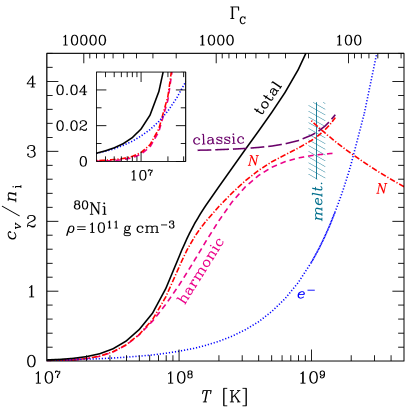
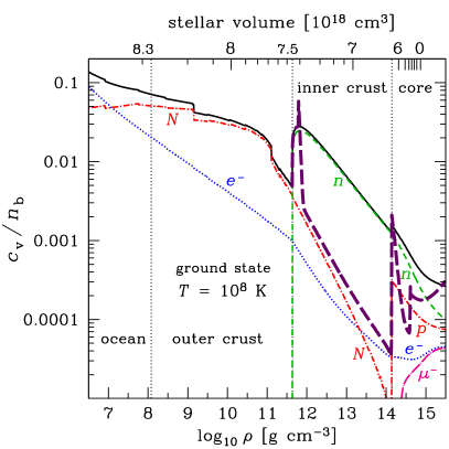
Figure 1: Left panel: Heat capacity per ion versus $T$ (bottom axis) and $\Gamma_{\mathrm{C}}$ (top axis) for ⁸⁰Ni at $\rho=10^{11}$ g cm^-3. The solid line displays the total normalized heat capacity $c_{\mathrm{v}}/n_{\mathrm{i}}$; the long-dashed line shows this quantity for a classical Coulomb lattice of ions, including harmonic and anharmonic terms; the short-dashed line is the harmonic-lattice approximation in the solid phase; the dot-dashed line is the same plus anharmonic and electron polarization corrections in the solid phase. The dotted line is the electron Fermi gas contribution. The vertical line is the OCP melting point $\Gamma_{\mathrm{C}}=175$, and the hatched band shows the range $\Gamma_{\mathrm{C}}=150$ – 200, where melting is expected to occur in realistic conditions. The inset illustrates the competition between the electron and ion contributions t low $T$. Right panel: Heat capacity per baryon as function of mass density from the ocean throughout the crust and core of a neutron star at $T=10^{8}$ K. The solid line displays the total $c_{\mathrm{v}}/n_{\mathrm{b}}$, and the other lines show its constituents due to the electrons ($e^{-}$), neutrons ($n$) in the inner crust and core, nuclei ($N$), including electrostatic terms in the ocean and crust but neglecting the neutron entrainment effects in the inner crust (Sect. 2.5.2), protons ($p$) and muons ($\mu^{-}$) in the core, assuming that the nucleons are non-superfluid. For comparison, the thick long dashes display an example of the total $c_{\mathrm{v}}/n_{\mathrm{b}}$ in the inner crust and core in the case of superfluid nucleons (Sect. 3.2). The top axis shows the volume contained inside a sphere with given $\rho$ for a 1.4 $M_{\odot}$ neutron star. The stellar structure and composition correspond to the BSk21 EoS model.

In Fig. 1 we show the temperature and density dependences of the normalized heat capacity of the ground-state matter in a neutron star. The left panel illustrates the dependence of $c_{\mathrm{v}}/n_{\mathrm{i}}$ on $T$, and the right panel the dependence of $c_{\mathrm{v}}/n_{\mathrm{b}}$ on $\rho$. Since the electron polarization effects shift the melting temperature (Sect. 2.4.1), the phase transition may occur anywhere within the hatched region around the vertical line $\Gamma_{\mathrm{C}}=175$ in the left panel.

When the temperature of the Coulomb liquid decreases, the heat capacity per ion increases from the ideal-gas value $c_{\mathrm{v,i}}/n_{\mathrm{i}}=\frac{3}{2}$ at $T\gg T_{\mathrm{m}}$ to, approximately, the simple harmonic lattice value $c_{\mathrm{v,i}}/n_{\mathrm{i}}=3$ at $T\lesssim T_{\mathrm{m}}$ (the Dulong-Petit law for a classical harmonic crystal). This gradual increase is due to the Coulomb non-ideality in the liquid phase, which effectively smears a phase transition between the strongly coupled Coulomb liquid and OCP crystal (see Baiko et al. 1998). With further cooling, quantum effects suppress the heat capacity. Once the crystal is deep into the quantum regime its specific heat is given by the Debye result

$$c_{\mathrm{v,i}}^{\mathrm{(D)}}=n_{\mathrm{i}}\frac{12\pi^{4}}{5}\left(\frac{T}{\Theta_{\mathrm{D}}}\right)^{3}.$$ (9)

The calculations of Baiko et al. (2001b) show that the Dulong-Petit law applies at temperatures down to $T\simeq T_{\mathrm{p}}$, while the Debye value of Eq. (9) is attained when $T\lesssim 0.1\,T_{\mathrm{p}}$. The same authors present a simple analytical approximation for the heat capacity of a harmonic Coulomb crystal, accurate to a few parts in $10^{5}$ at any $T$.

However, the harmonic OCP model is an idealization. The anharmonic corrections and electron polarization corrections (Sect. 2.4.1) can amount up to (10 – 20) % of $c_{\mathrm{v,i}}$. Because of the anharmonic effects, $c_{\mathrm{v,i}}/n_{\mathrm{i}}$ is not equal to 3 exactly, but is $\sim 10$% larger at $T=T_{\mathrm{m}}$. If the above-mentioned supercooling takes place in stellar matter, various fluid elements solidify at different $T$ below $T_{\mathrm{m}}$, and the average heat capacity, as function of temperature, can contain a bump, associated with latent heat releases (see Sect. 2.4.6 of Haensel et al. 2007 for a discussion).

The right panel of Fig. 1 shows the density dependence of the total heat capacity, normalized per one nucleon, $c_{\mathrm{v}}/n_{\mathrm{b}}$, throughout the neutron star from the ocean to the core, and partial contributions to $c_{\mathrm{v}}/n_{\mathrm{b}}$. Different particle fractions are adopted from the BSk21 model (Goriely et al. 2010; Pearson et al. 2011, 2012), as fitted by Potekhin et al. (2013). Here, we have mostly neglected the effects of nucleon superfluidity to be discussed in Sect. 3. The importance of these effects is demonstrated, however, by the heavy long-dashed line, which displays the total normalized heat capacity suppressed by nucleon superfluidity (see Sect. 3.2).

2.5.2 Specific heat of neutrons

In the inner crust, besides electrons and nuclei, there are also neutrons. In a thin layer at densities $\rho$ just above the neutron drip point $\rho_{\mathrm{drip}}$, the dripped neutrons are not paired (non-superfluid) and largely dominate $c_{\mathrm{v}}$. Heat capacity of strongly degenerate non-superfluid neutrons can be accurately evaluated using the above-referenced analytical fits, but since the neutrons are strongly degenerate almost everywhere in the neutron star, the simpler Sommerfeld result for Fermi gases at $T\ll\epsilon_{\mathrm{F}}$ is usually applicable,

$$c_{\mathrm{v,x}}\sim\frac{\pi^{2}}{2}\,\frac{n_{\mathrm{x}}\,T}{\epsilon_{\mathrm{F,x}}},$$ (10)

where x stands for the fermion type ($\textrm{x}=n,\,p,\,e,\,\mu$). For neutrons at $\rho$ only slightly above $\rho_{\mathrm{drip}}$, however, the latter formula is inaccurate because $\epsilon_{\mathrm{F},n}$ is not sufficiently large. For this reason, Pastore et al. (2015) proposed an interpolation between Eq. (10) and the ideal-gas limit $c_{\mathrm{v}}=\frac{3}{2}n$,

$$c_{\mathrm{v,x}}\approx\frac{3}{2}\,n_{\mathrm{x}}\left(1-\mathrm{e}^{-T/T_{\mathrm{cl}}}\right),\quad T_{\mathrm{cl}}=\frac{3\epsilon_{\mathrm{F,x}}}{\pi^{2}}.$$ (11)

They also showed that corrections due to the coupling to phonons (e.g., Sect. 1.4.4 in Baym and Pethick 1991) turn out to be unimportant for $c_{\mathrm{v},n}$. Approximation (11) is accurate within $17\%$ for non-relativistic Fermi gases at any density. For a relativistic Fermi gas, we can preserve this accuracy by using Eq. (5) for $\epsilon_{\mathrm{F,x}}$ and multiplying both $T_{\mathrm{cl}}$ and prefactor $\frac{3}{2}$ by the ratio $(mc^{2}+10T)/(mc^{2}+5T)$.

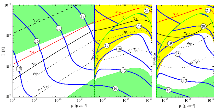
Figure 2: Iso-contour lines of $c_{\mathrm{v}}$ in the crust, labeled by the value of $\mathrm{log}_{10}(c_{\mathrm{v}}/\mathrm{erg\,cm^{-3}\,K^{-1}})$. Also shown are the melting curve $T_{\mathrm{m}}$ and the critical temperature for neutron ¹S₀ superfluidity, $T_{\mathrm{c}}$, the electron and ion plasma temperatures, $T_{\mathrm{p},e}$ and $T_{\mathrm{p}}$ respectively, the Debye temperature, $\Theta_{\mathrm{D}}\simeq 0.45T_{\mathrm{p}}$, that marks the transition from classical to quantum solid and $0.1T_{\mathrm{p}}$ below which the wholly quantum crystal regime is realized. The outer crust chemical composition is from Haensel and Pichon (1994) and inner crust from Negele and Vautherin (1973) with the neutron drip point at $\rho_{\mathrm{drip}}=4.3\times 10^{11}$ g cm ^-3. The electron contribution dominates in the two dark-shadowed (green) regions at high $T$ and $\rho$ below $\rho_{\mathrm{drip}}$ and at low $T$ and high $\rho$, while neutrons dominate in the light-shadowed (yellow) region at high $T$ and $\rho$ above $\rho_{\mathrm{drip}}$, and ions dominate in the intermediate regime. The right panel only displays the inner crust but assuming that about 80% of the dripped neutrons are entrained, illustrating the resulting increase in $c_{\mathrm{v,i}}$, mainly due to the strong reduction of $T_{\mathrm{p}}$ and $\Theta_{\mathrm{D}}$, significantly extending the regime where $c_{\mathrm{v,i}}$ dominates over $c_{\mathrm{v},e}$.

With further density increase, the neutrons become superfluid (Sect. 3), and then their contribution to $c_{\mathrm{v}}$ nearly vanishes. However, even in a superfluid state, the neutrons have a dramatic effect on $c_{\mathrm{v}}$. Indeed, Flowers and Itoh (1976) noticed that since free neutrons move in a periodic potential created by lattice of atomic nuclei, their energy spectrum should have a band structure, which can affect kinetic and neutrino emission phenomena involving the free neutrons. Chamel (2005) calculated the band structure of these neutrons, in much the same way as electron band structure is calculated in solid state physics. The effect of this band structure is that a large fraction of the dripped neutrons are “locked” to the nuclei, i.e., the thermal motion of the nuclei entrains a significant part of the dripped neutrons resulting in a strongly increased ion effective mass $m_{\mathrm{eff,i}}$. This increase $m_{\mathrm{i}}\rightarrow m_{\mathrm{eff,i}}$ significantly increases $c_{\mathrm{v,i}}$ in the quantum regime since $c_{\mathrm{v,i}}^{\mathrm{(D)}}\propto T_{\mathrm{p}}^{-1}\propto m_{\mathrm{i}}^{3/2}$ (Chamel et al. 2013).

The overall “landscape” of crustal specific heat is illustrated in Fig. 2. For highly degenerate electrons $c_{\mathrm{v},e}\propto T$, while for ions $c_{\mathrm{v,i}}$ decreases as $T^{3}$ according to Eq. (9), therefore the electron contribution dominates at $T\ll\Theta_{\mathrm{D}}$, and the ion contribution prevails at $T\gtrsim\Theta_{\mathrm{D}}$ (cf. the inset in the left panel of Fig. 1). On the other hand, in the non-degenerate regime $c_{\mathrm{v},e}/c_{\mathrm{v,i}}\sim Z$, therefore the contribution of the electrons dominates again for $Z>1$ at $T\gtrsim\epsilon_{\mathrm{F}}$ in the liquid phase (also cf. the left panel of Fig. 1). The effect of dripped neutron band structure on low-level collective excitations in the inner crust and the resulting increase of $c_{\mathrm{v,i}}$ is illustrated in the right panel of Fig. 2.

2.5.3 Specific heat of the core

The specific heat is simpler to evaluate in the core than in the crust but it has larger uncertainties. The core is a homogeneous quantum liquid of strongly degenerate fermions, and its specific heat is simply taken as the sum of its components contribution: $c_{\mathrm{v}}=\sum_{\mathrm{x}}c_{\mathrm{v,x}}$ where x stands for neutrons ($n$), protons ($p$), electrons ($e$), muons ($\mu$), and any other component as hyperons or quarks that may appear at high densities. For each fermionic component, one can use Eq. (10), but for baryons one should replace the bare fermion mass $m_{\mathrm{x}}$ by an effective mass $m_{\mathrm{x}}^{*}$, which encapsulates most effects of interactions. In principle, $m_{\mathrm{x}}^{*}$ should be calculated from the same microphysical interaction as employed for the EoS; cf. Sect. 2.6.3. For leptons ($e$ and $\mu$), interactions have a negligible effect on $m_{\mathrm{x}}^{*}$ and the bare fermion mass value can be used. The nucleon heat capacity in the core is strongly affected by pairing (superfluidity) effects, as discussed in Sect. 3.2.

2.6 Neutrino emissivity

The neutrino luminosity of a neutron star is, in most cases, strongly dominated by the core contribution, simply because the core comprises a lion’s share of the total mass. The crust contribution can, however, prevail in the case of strong superfluidity in the core, which suppresses the neutrino emissivities. Crust neutrino emission is also essential during the early thermal relaxation phase (the first few decades of the life of the star), or the crust relaxation after energetic transient events (e.g., strong bursts of accretion in X-ray binaries and flares in magnetars).

Yakovlev et al. (2001) reviewed the main neutrino emission mechanisms in neutron star crusts and cores and collected fitting formulae for the neutrino emissivity in each reaction as a function of density and temperature. The summary of the most important processes is given in Table 1. The last column of this table contains references to the analytical fitting formulae that can be directly employed to calculate the relevant emission rates. These processes are briefly described below.

Table 1: Main neutrino emission processes^a

	Process / Control function	Symbolic notationb	Formulae for $Q_{\nu}$ and/or $R$
In the crust
1	Plasmon decay	$\Gamma\to\nu+\bar{\nu}$	Eqs. (15) – (32) of [1]
2	Electron-nucleus bremsstrahlung	$e^{-}+N\to e^{-}+N+\nu+\bar{\nu}$	Eqs. (6), (16) – (21) of [2]
3	Electron-positron annihilation	$e^{-}+e^{+}\to\nu+\bar{\nu}$	Eq. (22) of [3]
4c	Electron synchrotron	$e^{-}\stackrel{{\scriptstyle B}}{{\to}}e^{-}+\nu+\bar{\nu}$	Eq. (48) – (57) of [3]
In the core
1d	Direct Urca (Durca)	$\begin{array}[]{l}n\rightarrow p+e^{-}+\bar{\nu}_{e}\,,\\ \,\,\,p+e^{-}\rightarrow n+\nu_{e}\end{array}$	Eq. (120) of [3]
	Magnetic modificationc	$R_{B}^{\mathrm{(D)}}$	Eqs. (247) – (250) of [3]
	Reduction factorse	$R_{x}^{\mathrm{(D)}}$	Eqs. (199), (202)–(206) of [3]
2	Modified Urca (Murca) (neutron branch)	$\begin{array}[]{l}n+n\rightarrow n+p+e^{-}+\bar{\nu}_{e}\,,\\ \,\,\,n+p+e^{-}\rightarrow n+n+\nu_{e}\end{array}$	Eq. (140) of [3]
	Reduction factorse	$R_{x}^{(\mathrm{M}n)}$	Appendix of [4]
3	Murca (proton branch)	$\begin{array}[]{l}p+n\rightarrow p+p+e^{-}+\bar{\nu}_{e}\,,\\ \,\,\,p+p+e^{-}\rightarrow p+n+\nu_{e}\end{array}$	Eq. (142) of [3], corrected at    $3p_{\mathrm{F}p}>p_{\mathrm{F}n}+p_{\mathrm{F}e}$ as per [4]
	Reduction factorse	$R_{x}^{(\mathrm{M}p)}$	Appendix (and Eq. (25)) of [4]
4	Baryon-baryon bremsstrahlung	$\left\{\begin{array}[]{l}n+n\rightarrow n+n+\nu+\bar{\nu}\\ n+p\rightarrow n+p+\nu+\bar{\nu}\\ p+p\rightarrow p+p+\nu+\bar{\nu}\end{array}\right.$	Eq. (165) of [3] Eq. (166) of [3] Eq. (167) of [3]
	Reduction factorse	$\left\{\begin{array}[]{l}R_{x}^{(nn)}\\[6.45831pt] R_{x}^{(np)}\\[7.74998pt] R_{x}^{(pp)}\end{array}\right.$	Eqs. (221), (222), (228) of [3]    and Eq. (60) of [4] Eq. (220), (229) of [3]    and Eq. (54) of [4] Eq. (221) of [3]
5e	Cooper pairing of baryons	$\left\{\begin{array}[]{l}n+n\to[nn]+\nu+\bar{\nu}\\ p+p\to[pp]+\nu+\bar{\nu}\end{array}\right.$	Eqs. (236), (241) of [3],    corrected as per [5] (Sect. 3.3)
6c,e	Electron-fluxoid bremsstrahlung	$e^{-}+f\to e^{-}+f+\nu+\bar{\nu}$	Eqs. (253), (263), (266) – (268)    of [3]

Notes. ^a References: [1] Kantor and Gusakov (2007); [2] Ofengeim et al. (2014); [3] Yakovlev et al. (2001); [4] Gusakov (2002); [5] Leinson (2009, 2010).   ^b $\Gamma$ means a plasmon, $e^{-}$ an electron, $e^{+}$ a positron, $\nu$ a neutrino, $\bar{\nu}$ an antineutrino (in general, of any flavor, but $\nu_{e}$ or $\bar{\nu}_{e}$ stands for the electron neutrino or antineutrino, respectively), $p$ a proton, $n$ a neutron, $[pp]$ and $[nn]$ their paired states, $N$ stands for an atomic nucleus, and $f$ for a proton fluxoid. At densities where muons are present, they participate in the Urca and bremsstrahlung processes fully analogous to the processes 1, 2, 3, 6 in the core (see details in Ref. [1]). $R$ with subscripts/superscripts signifies a control function (correction factor) due to superfluidity or magnetic field. Subscript $x$ in $R_{x}$ substitutes for different superfluidity types (proton or neutron, singlet or triplet); $B$ indicates magnetic field.   ^c The effect of strong magnetic field (see Sect. 4.3).   ^d At densities beyond the Durca threshold (see Sect. 2.6.2).   ^e The effect of superfluidity (see Sect. 3.3).

2.6.1 Neutrino emission in the crust

There is a variety of neutrino processes acting in the crust. In a non-magnetized crust the most important ones are the plasmon decay process and the electron-ion bremsstrahlung process (see Table 1). The pair annihilation process can be also important if the crust is sufficiently hot.

The total emissivity from the sum of these processes is illustrated in the left panel of Fig. 3. The first thing to notice is the enormous range of values of $Q_{\nu}$ covered in the $\rho-T$ range displayed in this figure, which spans 26 orders of magnitude. This is a direct consequence of the strong $T$ dependence of the neutrino processes. The pair annihilation process is efficient only at low densities and very high temperatures, but when $T\ll T_{\mathrm{F,e}}$ very few positrons are present and the process is strongly suppressed. In the whole range of this plot, $T_{\mathrm{F,e}}\gg 10^{10}$ K but pair annihilation still dominates at low $\rho$ and high $T$. In the opposite high-$\rho$ and low-$T$ regime the dominant process is electron-ion bremsstrahlung, for which $Q_{\nu}^{\mathrm{(brems)}}\propto T^{8}$. At intermediate $T$ and $\rho$ the plasmon decay process is most important and, when it strongly dominates, its emissivity behaves as $Q_{\nu}^{\mathrm{(pl)}}\propto T^{4}$.

The right panel of Fig. 3 illustrates the density dependence of $Q_{\nu}^{(\mathrm{pl})}$ and $Q_{\nu}^{(\mathrm{brems})}$ in either ground-state or accreted crust of a neutron star with $T=10^{9}$ K. Pair annihilation is negligible in this case. $Q_{\nu}^{(\mathrm{pl})}$ is calculated according to Yakovlev et al. (2001) and $Q_{\nu}^{(\mathrm{brems})}$ according to Ofengeim et al. (2014). For comparison, an older fit to $Q_{\nu}^{(\mathrm{brems})}$ (Kaminker et al. 1999) is plotted by the dotted line. The ground-state composition and the nuclear size are described by the BSk21 model (Goriely et al. 2010; Pearson et al. 2012, as fitted by Potekhin et al. 2013). The accreted composition is taken from Haensel and Zdunik (1990); in this case the approximation by Itoh and Kohyama (1983) is used for the nuclear size.

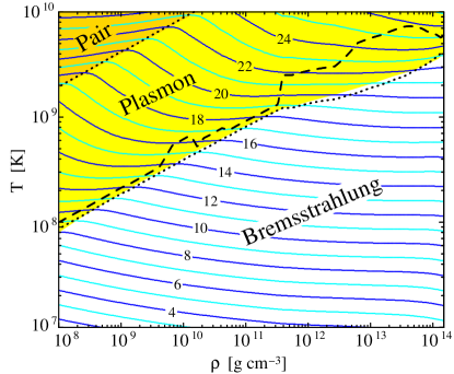
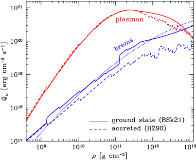
Figure 3: Neutrino emissivity $Q_{\nu}$ in a non-magnetized crust from the pair annihilation, plasmon decay, and electron-ion bremsstrahlung processes. Left panel: The contour lines are labeled by the value of $\mathrm{log}_{10}[Q_{\nu}/(\mathrm{erg\,cm}^{-3}\,\mathrm{s}^{-1})]$. Regions where the pair, plasma, and bremsstrahlung processes dominate are indicated: the boundaries happen to be quite well described by the two dotted lines that show $\frac{5}{3}T_{\mathrm{p},e}$ and $\frac{1}{13}T_{\mathrm{p},e}$. (Also indicated is the ion melting curve, dashed line.) Right panel: Density dependences of $Q_{\nu}$ for the ground-state nuclear matter (solid lines) and for the accreted crust (dashed lines) at $T=10^{9}$ K. The dotted line represents an older fit to the bremsstrahlung process (see text for detail).

The band structure of the energy spectrum of neutrons in the inner crust, which was mentioned in Sect. 2.5.1, should reduce the neutrino reactions of the bremsstrahlung type and initiate an additional neutrino emission due to direct inter-band transitions of the neutrons, in analogy with Cooper pairing of neutrons discussed in Sect. 3.3. These effects have been mentioned by Yakovlev et al. (2001), but remain unexplored.

Electron and positron captures and decays by atomic nuclei (beta processes), which accompany cooling of matter and non-equilibrium nuclear reactions, produce neutrino emission. A pair of consecutive beta capture and decay reactions is a nuclear Urca process. Urca processes involving electrons were put forward by Gamow and Schoenberg (1941), while those involving positrons were introduced by Pinaev (1964). In the neutron star crust, the appropriate neutrino luminosity depends on cooling rate and should be especially strong at $T\sim$(2–4) $\times 10^{9}$ K when the main fraction of free neutrons is captured by nuclei. However, there are other efficient neutrino reactions open at such temperatures, which make the neutrino emission due to beta processes insignificant (Yakovlev et al. 2001). On the other hand, heating produced by non-equilibrium nuclear reactions (the deep crustal heating, Haensel and Zdunik 1990) that accompany accretion mentioned in Sect. 2.4.1, may be more important than non-equilibrium neutrino cooling.

There are a number of other neutrino-emission processes (Yakovlev et al. 2001), which are less efficient than those listed in Table 1. In the inner crust with dripped neutrons, $n-n$ bremsstrahlung is very efficient but it is suppressed by pairing and, hence, only acts in the layers where $T>T_{\mathrm{c}n}$, where $T_{\mathrm{c}n}$ is the neutron pairing critical temperature (Sect. 3.1). This process operates in a wide range of densities and temperatures, and the density dependence of its emissivity is generally smooth. Neutrino emission from the formation and breaking of Cooper pairs makes a significant contribution, much stronger than the bremsstrahlung, but is confined to a restricted region of $\rho$ and $T$ (Sect. 3.3). In the presence of a very strong magnetic field, some of the above-mentioned processes are modified, and new channels for neutrino emission may open (Sect. 4).

2.6.2 Neutrino emission in the core

Yakovlev et al. (2001) discussed a wealth of neutrino reactions which may be important in the $npe\mu\Lambda\Sigma^{-}$ matter in a neutron star core, which include

• 8 direct Urca (Durca) processes of the electron or muon production and capture by baryons (baryon direct Urca processes),

• 32 modified Urca (Murca) processes, also associated with the electron or muon production and capture by baryons (baryon Murca processes),

• 12 processes of neutrino-pair emission in strong baryon-baryon collisions (baryon bremsstrahlung),

• 4 Murca processes associated with muon decay and production by electrons (lepton Murca process),

• 7 processes of neutrino pair emission in Coulomb collisions (Coulomb bremsstrahlung).

In this paper we basically restrict ourselves to the $npe\mu$ matter. We refer the reader to the review by Yakovlev et al. (2001) for the more general case, as well as for a discussion of other exotic models (such as the pion or kaon condensates). It appears that the reactions that proceed in the $npe\mu$ matter are often sufficient for the neutron-star cooling, even when the appearance of the $\Sigma^{-}$ and $\Lambda$ hyperons is allowed. The reason is that these hyperons can appear at high densities only, where the baryon Durca processes are likely to be allowed and dominate, for realistic EoSs.

The Durca cycle consists of the beta decay and electron capture processes (see Table 1). They are threshold reactions open at sufficiently high densities, and not for every EoS model. For the degenerate nucleons they are only possible if the proton fraction exceeds a certain threshold. In the $npe$ matter (without muons) this threshold is $\approx 11\%$, which follows readily from the energy and momentum conservation combined with the condition of electric charge neutrality of matter. Indeed, for strongly degenerate fermions the Pauli blocking implies that the reaction is possible only if the energies of the reacting particles are close to their respective Fermi energies. Then the momentum conservation assumes the inequality $p_{\mathrm{Fn}}\leqslant{p}_{\mathrm{Fe}}+{p}_{\mathrm{Fp}}$, that is $n_{n}^{1/3}\leqslant n_{e}^{1/3}+n_{p}^{1/3}$. For the $npe$ matter $n_{e}=n_{p}$ because of the charge neutrality, therefore $n_{n}\leqslant 8n_{p}$, or $n_{p}\geqslant n_{\mathrm{b}}/9$, where $n_{\mathrm{b}}$ is the total baryon number density. The presence of muons can increase this threshold by several percent. If ${p}_{\mathrm{F\mu}}\geqslant{p}_{\mathrm{Fn}}-{p}_{\mathrm{Fp}}$, then the muon Durca process adds to the electron Durca.

If allowed, the Durca processes produce a rapid (enhanced) cooling of neutron stars. If they are forbidden, the main reactions are those of the baryon Murca and bremsstrahlung processes which produce a slow (standard) cooling. The Murca process is a second order process, in which a bystander neutron or proton participates to allow momentum conservation (see Table 1). Since this process involves five degenerate fermions, instead of three for the Durca process, its efficiency is reduced, simply by phase space limitation, by a factor of order $(T/\epsilon_{\mathrm{F}})^{2}$, which gives an overall temperature-dependence $T^{8}$ instead of $T^{6}$. This reduction, for typical conditions in the neutron-star core, amounts to 6 orders of magnitude. It is certainly the dominant process for not too high densities in absence of pairing, and is the essence of the “standard cooling scenario”. However, in presence of superfluidity, neutrino emission by the formation of Cooper pairs (Sect. 3.3) can dominate over the Murca process.

Other neutrino reactions in the core involve neutrino-pair bremsstrahlung in Coulomb collisions lepton modified Urca processes, electron-positron annihilation, etc. All of them are not significant under the typical conditions in the non-exotic core. For instance, the plasmon decay process that is efficient in the neutron star crust (Sect. 2.6.1) is exponentially suppressed in the core, because the electron plasmon energy in the core ($\sim\hbar\omega_{\mathrm{p}}\sim 10$ MeV) is much larger than the thermal energy.

In a strong magnetic field penetrating into the core, some of the above-mentioned processes can be modified, and new channels for neutrino emission may open (see Sect. 4).

2.6.3 Remarks on in-medium effects

Neutrino emissivity $Q_{\nu}$ may be strongly modified by in-medium (collective) effects at the high densities of neutron stars (see Voskresensky 2001, for a review). For instance, these effects may result in renormalization of electroweak interaction parameters. Moreover, the in-medium effects may open new channels for neutrino emission. Voskresensky and Senatorov (1986) found that the direct and modified Urca processes appreciably exceed the estimates obtained neglecting the collective effects, provided the density is sufficiently large. On the other hand, the in-medium effects suppress the $nn$ bremsstrahlung in the neutron-star core by a factor of 10 – 20 (Blaschke et al. 1995). According to the study by Schaab et al. (1997), the medium effects on the emissivity of the Murca process cause a more rapid cooling than obtained for the standard scenario and result in a strong density dependence, which gives a smooth crossover from the standard to the enhanced cooling scenario (see Sect. 6.1) for increasing star masses.

The problem of calculation of the in-medium effects in the neutron star matter is complicated. Various theoretical approaches were used to solve it, results of different techniques being different typically by a factor of a few (see, e.g., Blaschke et al. 1995, and references therein). The renormalization of the electroweak coupling is usually taken into account in an approximate manner by replacing the bare baryon masses $m_{B}$ with effective ones, $m_{B}^{*}$ (e.g., Yakovlev et al. 2001). The values of these effective masses should be taken from microscopic theories.

The in-medium effects are also important for the Cooper-pairing neutrino emission mechanism related to baryon superfluidity, as discussed in Sect. 3.3 below, for heat capacity (Sect. 2.5.3), and for baryon heat conduction (Sect. 2.7.3) in the core of a neutron star.

2.7 Thermal conductivity

The most important heat carriers in the crust and ocean of the star are the electrons. In the atmosphere, the heat is carried mainly by photons. In general, the two mechanisms work in parallel, hence $\kappa=\kappa_{\mathrm{r}}+\kappa_{e},$ where $\kappa_{\mathrm{r}}$ and $\kappa_{e}$ denote the radiative (r) and electron (e) components of the thermal conductivity $\kappa$. The radiative transfer is considered in Paper I. In this paper we will pay most attention to the electron heat conduction mechanism. Both the electron and photon heat conduction are affected by strong magnetic fields. We will consider these effects in Sect. 4.

The elementary theory in which the effective collision rate $\nu$ of heat carriers with effective mass $m^{*}$ and number density $n$ does not depend on their velocity, gives (Ziman 1960)

$$\kappa=a\,{nT}/{m^{\ast}\nu},$$ (12)

where $a$ is a numerical coefficient: $a=3/2$ for a non-degenerate gas, and $a=\pi^{2}/3$ for strongly degenerate particles. (We remind that we use energy units for $T$; otherwise $a$ should be multiplied by the squared Boltzmann constant.)

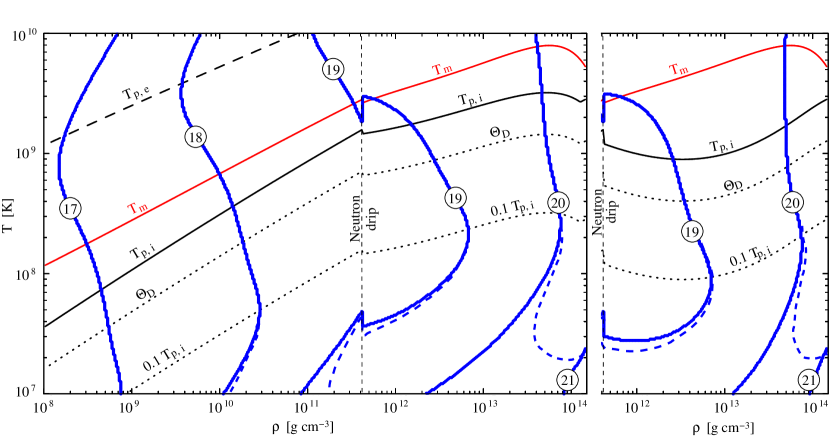
Figure 4: Iso-contour lines of the electron thermal conductivity $\kappa_{e}$ in the crust, labeled by the value of $\mathrm{log}_{10}(\kappa_{e}/\mathrm{erg\,s^{-1}\,cm^{-1}\,K^{-1}})$, using the results of Gnedin et al. (2001). Also shown are the melting curve $T_{\mathrm{m}}$, the electron and ion plasma temperatures, $T_{\mathrm{p},e}$ and $T_{\mathrm{p}}$ respectively, the Debye temperature, $\Theta_{\mathrm{D}}\simeq 0.45T_{\mathrm{p}}$, that marks the transition from classical to quantum solid and $0.1T_{\mathrm{p}}$ below which the wholly quantum crystal regime is realized. The crust composition is the same as in Fig. 2. The right panel only displays the inner crust but assuming that about 80% of the dripped neutrons are entrained: the strong reduction of $T_{\mathrm{p}}$ and $\Theta_{\mathrm{D}}$ pushes the onset of the wholly quantum regime to lower $T$. The dashed contour lines illustrate the reduction of $\kappa_{e}$ from impurity scattering, assuming an impurity parameter $Q_{\mathrm{imp}}=1$.

The most important heat carriers and respective scattering processes that control the thermal conductivity $\kappa$ are listed in Table 2, and briefly discussed below. The last column of the table contains references to either analytical fitting formulae or publicly available computer codes for the evaluation of $\kappa$. Figure 4 illustrates the magnitude of $\kappa_{e}$ and characteristic temperatures in the crust.

Table 2: Main contributions to thermal conductivity

	Conduction type and regime	Referencesa
1b	Photon conduction	Eqs. (14) – (20) of [1]
	– plasma cutoff correction	Sect. 3.3 of [2]
	– magnetic field modificationsc	Eqs. (21) – (23) of [1]
2	Electron conduction in the ocean and the crust:	see Appendix A.
	– Electron-ion / electron-phonon scattering	[3] (theory), [4] (public code)
	– the effects of magnetic fieldsd	[5] (theory), [4] (public code)
	– the effects of finite nuclear sizes in the inner crust	[6] (theory), [4] (public code)
	– Electron scattering on impurities in the crust	see Appendix A.4
	– Electron-electron scattering:
	– strongly degenerate electrons	Eqs. (10), (21) – (23) of [7]
	– arbitrary degeneracy	see Appendix A.3
3	Baryon conduction in the core	Eqs. (7), (12), (21), (28) – (30) of [8]
	– Effects of superfluiditye	Eqs. (45) – (48), (50) – (53) of [8]
4	Lepton conduction in the core	Eqs. (4) – (6), (16), (17), (33) – (37) of [9]
	– Effects of superfluiditye	Eqs. (45), (54) – (61), (84) – (92)f of [9]

Notes. ^a References: [1] Potekhin and Yakovlev (2001); [2] Potekhin et al. (2003); [3] Potekhin et al. (1999); [4] http://www.ioffe.ru/astro/conduct/; [5] Potekhin (1996, 1999); [6] Gnedin et al. (2001); [7] Shternin and Yakovlev (2006); [8] Baiko et al. (2001a); [9] Shternin and Yakovlev (2007).   ^b For fully ionized atmospheres only. For partially ionized atmospheres, see references in Potekhin (2014).   ^c See Sect. 4.4.1.   ^d See Sect. 4.4.2.   ^e See Sect. 3.4.   ^f The power index 2 should be suppressed at its first occurrences in the third and fourth lines of Eq. (92) of Ref. [9].

2.7.1 Heat conduction in the outer envelopes

Electron heat conduction is the most important process in the neutron star envelopes that determines thermal luminosity of neutron stars. In this case, $m^{\ast}=m_{e}\,\sqrt{1+x_{\mathrm{r}}^{2}}$ in Eq. (12), and $\nu=\nu_{e}$ is mostly determined by electron-ion ($e$i) and electron-electron ($ee$) Coulomb collisions. In the crystalline phase, the electron-ion scattering takes the form of scattering on phonons (collective ion excitations). The Matthiessen rule (e.g., Ziman 1960) assumes that effective frequencies of different collisions simply add up, i.e., $\nu_{e}=\nu_{e\mathrm{i}}+\nu_{ee}$. This is strictly valid for extremely degenerate electrons (Hubbard and Lampe 1969). In general case it remains a good estimate, because $\nu_{e\mathrm{i}}+\nu_{ee}\leq\nu_{e}\leq\nu_{e\mathrm{i}}+\nu_{ee}+\delta\nu$, where $\delta\nu\ll\min(\nu_{e\mathrm{i}},\nu_{ee})$ (Ziman 1960). The relative importance of the different types of collisions and practical formulae for evaluation of $\nu_{e}$ can be different, depending on the composition and phase state of the plasma (see Appendix A.).

Chugunov and Haensel (2007) considered an alternative heat transport by the plasma ions (phonons in the solid OCP), which works in parallel with the transport by the electrons. The ion (phonon) heat conduction is usually unimportant in neutron stars. Although the ion thermal conductivity can be larger than the electron conductivity across the strong magnetic field, the multidimensional modeling shows that in such cases the heat is mainly transported by the electrons non-radially (i.e., not straight across the field lines; see Sect. 6).

2.7.2 Heat conduction in the inner crust

The inner crust of a neutron star is characterized by the presence of free neutrons. This has two important consequences. First, heat transport by neutrons can compete with the transport by the electrons and phonons. Second, electron-neutron scattering adds to the other electron scattering mechanisms considered above and in Appendix A..

The thermal conductivity by neutrons, $\kappa_{n}$, was studied in several papers (e.g., Flowers and Itoh 1976; Bisnovatyi-Kogan and Romanova 1982). A general expression for $\kappa_{n}$ in non-superfluid matter is given by Eq. (12) with $n=n_{n}$, the number density of neutrons, $m^{*}=m_{n}^{\ast}$, the neutron effective mass modified by medium effects, and $\nu_{n}=\nu_{n\mathrm{i}}+\nu_{nn}$. The neutron-neutron collision frequency, $\nu_{nn}$, can be calculated in the same manner as in uniform matter of a neutron-star core (Sect. 2.7.3). However, for strongly degenerate neutrons these collisions are much less efficient than the neutron-ion ones. Therefore, one can set $\nu_{n}\approx\nu_{n\mathrm{i}}$, at least for order-of-magnitude estimates. For the scattering of the neutrons by uncorrelated nuclei, $\nu_{n\mathrm{i}}=n_{\mathrm{i}}\,\mathrm{v}_{\mathrm{F}n}\,S_{n\mathrm{i}}$, where $\mathrm{v}_{\mathrm{F}n}=p_{\mathrm{F}n}/\sqrt{c^{2}+(p_{\mathrm{F}n}/m_{n}^{\ast})^{2}}$ is the neutron Fermi velocity and $S_{n\mathrm{i}}$ is the transport cross section. For a crude estimate at sufficiently low neutron energies in the neutron star crust one can set (e.g., Bisnovatyi-Kogan and Romanova 1982) $S_{n\mathrm{i}}=\pi\,R_{n}^{2}$, where $R_{n}$ is the neutron radius of an atomic nucleus (fitted, e.g., in Potekhin et al. 2013). Estimated in this way, $\kappa_{n}$ is negligible, being at least two orders of magnitude smaller than $\kappa_{e}$ in the entire inner crust at $T\lesssim 10^{9}$ K. However, $\nu_{n\mathrm{i}}$ can be strongly affected by ion-ion correlations and by superfluidity (Sect. 3.4).

In addition, the electron conduction in the inner crust is affected by the size of a nucleus, which becomes non-negligible compared to the mean distance between the nuclei, so that the approximation of pointlike scatterers is not applicable anymore. Then one should take into account the form factor, which depends on the size and shape of the charge distribution in a nucleus. A finite charge distribution reduces $\nu_{e\mathrm{i}}$ with respect to the model of a pointlike charge, thereby increasing the conductivity (Gnedin et al. 2001). The effect mainly depends on the ratio of the root mean square charge radius of a nucleus $R_{\mathrm{ch}}$ to the Wigner-Seitz cell radius $a_{\mathrm{i}}$. Gnedin et al. (2001) presented fitting formulae for the dependences of the thermal and electrical conductivities on the parameter $x_{\mathrm{nuc}}=\sqrt{5/3}\,R_{\mathrm{ch}}/a_{\mathrm{i}}$. The latter parameter has been fitted as function of density for modern BSk models of nuclear matter (Potekhin et al. 2013) and for some other models (Appendix B in Haensel et al. 2007).

2.7.3 Heat conduction in the core

The first detailed studies of the kinetic coefficients in neutron star cores were performed by Flowers and Itoh (1979), who constructed the exact solution of the multicomponent system of transport equations in the $npe$ matter. But since the proton fraction is small and the electron-neutron interaction is weak, the kinetic coefficients can be split in two almost independent parts – the neutron kinetic coefficients mediated by nucleon-nucleon collisions and electron kinetic coefficients mediated by the collisions between charged particles; the proton kinetic coefficients are small. In the non-superfluid $npe\mu$ matter, the neutrons are the main heat carriers at $T\lesssim 10^{8}$ K, while the heat transport by leptons $e^{-}$ and $\mu^{-}$ is competitive at $T\gtrsim 10^{9}$ K (Shternin and Yakovlev 2007; Shternin et al. 2013).

Baryon heat conduction.

Flowers and Itoh (1979) based their calculations on the free nucleon scattering amplitudes, neglecting the Fermi-liquid effects and nucleon many-body effects. Their results were later reconsidered by Baiko et al. (2001a).

The thermal conductivity is written in the form analogous to Eq. (12):

$$\kappa_{n}=\frac{\pi^{2}Tn_{e}\tau_{n}}{3m_{n}^{*}},\quad\kappa_{p}=\frac{\pi^{2}Tn_{p}\tau_{p}}{3m_{p}^{*}},$$ (13)

where the effective relaxation times $\tau_{n}$ and $\tau_{p}$ are provided by solution of the system of algebraic equations (e.g., Shternin et al. 2013)

$$\sum_{j=n,p}\nu_{ij}\tau_{j}=1,\qquad\nu_{ij}=\frac{64m_{i}^{*}m_{j}^{*2}T^{2}}{5m_{N}^{2}\hbar^{3}}\,S_{ij}\qquad(i,j=n,p),$$ (14)

where $\nu_{ij}$ are effective collision frequencies, $m_{N}$ is the bare nucleon mass in vacuo, and $S_{ij}$ are the effective cross-sections.

Many-body effects in the context of transport coefficients of pure neutron matter were first addressed by Wambach et al. (1993) and later reconsidered in many papers. There are two kinds of these effects: the three-body part of the effective potential for the nucleon-nucleon interactions and the in-medium effects (cf. Sect. 2.6.3) that affect nucleon-nucleon scattering cross-sections. Baiko et al. (2001a) calculated $S_{ij}$ in the approximation of pairwise interactions between nucleons with appropriate effective masses, using the Bonn potential model for the elastic nucleon-nucleon scattering (Machleidt et al. 1987) with and without the in-medium effects. They presented the results in the form $S_{ij}=S_{ij}^{(0)}K_{ij},$ where $S_{ij}^{(0)}$ corresponds to scattering of bare particles, and $K_{ij}$ describes the in-medium effects. They also constructed a simple analytical fits to their results for $S_{ij}^{(0)}$ and $K_{ij}$ (referenced in Table 2).

Shternin et al. (2013) studied the many-body effects on the kinetic coefficients of nucleons in the $npe\mu$ matter in beta equilibrium using the Brueckner-Hartree-Fock (BHF) method. According to this study, the three-body forces suppress the thermal conductivity. This suppression is small at low densities but increases to a factor of $\sim 4$ at the baryon number density of $n_{\mathrm{b}}=0.6$ fm^-3. However, the use of the effective masses partly grasps this difference. For this reason it proves to be sufficient to multiply the conductivities obtained in the effective-mass approximation (Baiko et al. 2001a) by a factor of 0.6 to reproduce the BHF thermal conductivity (Shternin et al. 2013) with an accuracy of several percent in the entire density range of interest.

Lepton heat conduction.

The up-to-date electron and muon contributions to thermal conductivities of neutron star cores were calculated by Shternin and Yakovlev (2007). Their treatment included the Landau damping of electromagnetic interactions owing to the exchange of transverse plasmons. This effect was studied by Heiselberg and Pethick (1993) for a degenerate quark plasma, but was neglected in the previous studies of the lepton heat conductivities in the $npe\mu$ matter (e.g., Flowers and Itoh 1981; Gnedin and Yakovlev 1995).

The electron and muon thermal conductivities are additive, $\kappa_{e\mu}=\kappa_{e}+\kappa_{\mu}$, and can be written in the familiar form of Eq. (12):

$$\kappa_{e}=\frac{\pi^{2}Tn_{e}\tau_{e}}{3m_{e}^{*}},\quad\kappa_{\mu}=\frac{\pi^{2}Tn_{\mu}\tau_{\mu}}{3m_{\mu}^{*}},$$ (15)

where $\kappa_{e}$ and $\kappa_{\mu}$ are the partial thermal conductivities of electrons and muons, respectively; $n_{e}$ and $n_{\mu}$ are number densities of these particles, $m_{e}^{*}$ and $m_{\mu}^{*}$ are their dynamical masses at the Fermi surfaces, determined by their chemical potentials. In neutron star cores at beta equilibrium these chemical potentials are equal, therefore $m_{e}^{*}=m_{\mu}^{*}$. The effective electron and muon relaxation times can be written as (Gnedin and Yakovlev 1995)

$$\tau_{e}=\frac{\nu_{\mu}-\nu^{\prime}_{e\mu}}{\nu_{e}\nu_{\mu}-\nu^{\prime}_{e\mu}\nu^{\prime}_{\mu e}},\quad\tau_{\mu}=\frac{\nu_{e}-\nu^{\prime}_{\mu e}}{\nu_{e}\nu_{\mu}-\nu^{\prime}_{e\mu}\nu^{\prime}_{\mu e}},$$ (16)

where $\nu_{e}=\sum_{i}\nu_{ei}=\nu_{ee}+\nu_{e\mu}+\nu_{ep}$ and $\nu_{\mu}=\sum_{i}\nu_{\mu i}=\nu_{\mu\mu}+\nu_{\mu e}+\nu_{\mu p}$ are the total effective collision frequencies of electrons and muons with all charged particles $i=e,\mu,p$; $\nu_{ei}$ and $\nu_{\mu i}$ are partial effective collision frequencies, while $\nu^{\prime}_{e\mu}$ and $\nu^{\prime}_{\mu e}$ are additional effective collision frequencies, which couple heat transport of the electrons and muons. All these collision frequencies can be expressed as multidimensional integrals over momenta of colliding particles. Shternin and Yakovlev (2007) calculated these integrals in the weak-screening approximation and described the results by simple analytical formulae (referenced in Table 2). In the case of strongly degenerate ultra-relativistic leptons, which is typical for neutron star cores, the latter authors obtained a much simpler expression, which can be written as

$$\kappa_{e,\mu}\approx 20.8\,c\,({p_{\mathrm{F}}}_{e,\mu}/\hbar)^{2}.$$ (17)

The latter simplification, however, does not hold if the protons are superfluid.

3 Superfluidity and superconductivity

Soon after the development of the BCS theory (Bardeen et al. 1957), which explains superconductivity by Cooper pairing of fermions (Cooper 1956), Bohr et al. (1958) argued that the same phenomenon of pairing is occurring inside nuclei (later this suggestion was confirmed experimentally). Migdal (1959) extended the idea to the interior of neutron stars. Ginzburg and Kirzhnits (1965) formulated a number of important propositions concerning neutron superfluidity in the interior of neutron stars, the formation of Feynman-Onsager vortices, a critical superfluidity temperature ($T_{\mathrm{c}}\lesssim 10^{10}$ K) and its dependence on the density ($\rho\sim 10^{13}$ – $10^{15}$ g cm^-3), and discussed the influence of neutron superfluidity on heat capacity and therefore on the thermal evolution of a neutron star. Baym et al. (1969) and Ginzburg (1970) analyzed the consequences of neutron superfluidity and proton superconductivity: rotation of the superfluid component in the form of quantized vortices and splitting of the internal stellar magnetic field into fluxoids (Sect. 4.3.4). Later many different authors considered various types of pairing of nucleons, hyperons, or quarks using different model potentials.

Although we will not consider exotic models of neutron star cores, let us mention that superfluidity is possible in these models as well. For instance, Takatsuka and Tamagaki (1995) reviewed calculations of neutron and proton superfluid gaps in pion condensed matter. Some authors have discussed superfluidity in quark matter (e.g., Stejner et al. 2009). If hyperons are present, they can also be in a superfluid state (Balberg and Barnea 1998). For a detailed recent review of superfluidity in the interiors of neutron stars, see Page et al. (2014).

3.1 Pairing types and critical temperatures

The Cooper pairing appears as a result of the attraction of particles with the anti-parallel momenta,which is expected to occur, at low enough temperature, in any degenerate system of fermions in which there is an attractive interaction between particles whose momenta $\bm{p}$ lie close to the Fermi surface (Cooper 1956). The strength of the interaction determines the critical temperature $T_{\mathrm{c}}$ at which the pairing phase transition will occur. In a normal system the particle energy $\epsilon$ varies smoothly when the momentum crosses the Fermi surface, while in the presence of pairing a discontinuity develops, with a forbidden energy zone having a minimum width of $2\Delta_{\mathrm{pair}}$ at $p=p_{\mathrm{F}}$, which can be regarded as the binding energy of a Cooper pair.

The BCS equations that describe symmetric nuclear matter in atomic nuclei and asymmetric neutron-rich matter in neutron stars have much in common but have also some differences. For instance, pairing in atomic nuclei takes place in the singlet state of a nucleon pair. In this case, the energy gap is isotropic, that is independent of the orientation of nucleon momenta. On the other hand, one can expect triplet-state pairing in the neutron-star matter, which leads to anisotropic gap. Singlet-state neutron superfluidity develops in the inner neutron star crust and disappears in the core, where an effective neutron-neutron singlet-state attraction transforms into repulsion. Triplet-state neutron superfluidity appears in the neutron-star core. Protons in the core can undergo the singlet-state pairing.

The triplet pair states may have different projections $m_{J}$ of the total pair momentum onto the quantization axis: $|m_{J}|=0$, 1, and 2. The actual (energetically favorable) state may be a superposition of states with different $m_{J}$. Owing to uncertainties of microscopic theories this state is still unknown; it depends possibly on density and temperature. In simulations of neutron star cooling, one usually considers the triplet-state pairing with $|m_{J}|=0$ and 2, since their effects on the heat capacity and neutrino luminosity are qualitatively different (e.g., Yakovlev et al. 1999b, 2001).

The critical temperature $T_{\mathrm{c}}$ is very sensitive to the strength of the repulsive core of the nucleon-nucleon interaction. It is related to the superfluid energy gap by $T_{\mathrm{c}}=0.5669\Delta_{\mathrm{pair}}$ for the singlet gap (e.g., Lifshitz and Pitaevskiĭ 2002, Sect. 40). For the triplet gap, the situation is more complicated, because the gap is anisotropic (e.g., Amundsen and Østgaard 1985b; Baldo et al. 1992; Yakovlev et al. 1999b). Examples of the dependence of $T_{\mathrm{c}}$ on gravitational mass density in the crust and core of a neutron star are shown in Fig. 5. Here, we employed the gap parametrization of Kaminker et al. (2001) with the parameter values and notations for different models of superfluidity according to Ho et al. (2015) together with the $\rho$-dependences of free-nucleon number densities $n_{n}$ and $n_{p}$ from the fits (Potekhin et al. 2013) for the BSk21 model of crust and core composition. Figure 5 demonstrates a large scatter of theoretical predictions, but also general features. We see that the ¹S₀ superfluidity of neutrons occurs mostly in the inner crust and the ³P₂ superfluidity mostly in the core. The critical temperatures of neutrons in the triplet states, $T_{\mathrm{c}n}(\mbox{${}^{3}$P${}_{2}$})$, and protons, $T_{\mathrm{c}p}(\mbox{${}^{1}$S${}_{0}$ })$, have usually a maximum at a supranuclear density $\rho>\rho_{0}$. Typical magnitudes of $T_{\mathrm{c}}$ vary from one model to another within a factor of a few. Neutron ³P₂ superfluidity has, in general, much lower $T_{\mathrm{c}}$ than ¹S₀ pairing of neutrons in the inner crust and protons in the core.

3.2 Superfluid effects on heat capacity

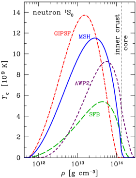
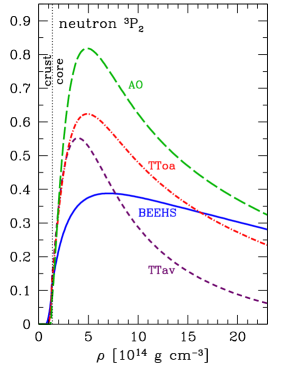
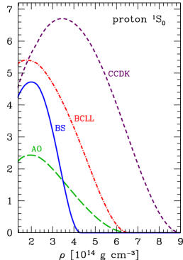
Figure 5: Critical temperatures of singlet neutron (left panel), triplet neutron (middle panel), and singlet proton (right panel) superfluidities in the inner crust and core of a neutron star, as functions of gravitational mass density $\rho$, for different superfluidity models, as marked near the curves (see Ho et al. 2015): AO (Amundsen and Østgaard 1985a, b), AWP2 (Ainsworth et al. 1989), BCLL (Baldo et al. 1992), BEEHS (Baldo et al. 1998), BS (Baldo and Schulze 2007), CCDK (Chen et al. 1993), GIPSF (Gandolfi et al. 2008), MSH (Margueron et al. 2008), SFB (Schwenk et al. 2003), TTav and TToa (Takatsuka and Tamagaki 2004).

Once a component x of the neutron star matter becomes superfluid, its specific heat $c_{\mathrm{v,x}}$ is strongly altered. When $T$ reaches $T_{\mathrm{c,x}}$, the critical temperature for the pairing phase transition, $c_{\mathrm{v,x}}$ jumps by a factor $\gtrsim 2$. However, as $T$ continues to decrease, the heat capacity becomes progressively suppressed. At $T\ll T_{\mathrm{c}}$ the energy gap in the nucleon spectrum strongly reduces the heat capacity even compared to its value in the absence of pairing. These effects are implemented in numerical calculations through “control functions” $R_{\mathrm{c}}(T/T_{\mathrm{c,x}})$ as

$$c_{\mathrm{v,x}}=R_{\mathrm{c}}\,c_{\mathrm{v,x}}^{(0)},$$ (18)

where $c_{\mathrm{v,x}}^{(0)}$ denotes the value in the normal phase, Eq. (10). The control function depends on the type of pairing. This dependence was studied by Levenfish and Yakovlev (1994). Analytical fitting formulae for $R_{\mathrm{c}}$ in the $npe\mu$ matter for the main types of superfluidity listed above are given by Eq. (18) of Yakovlev et al. (1999b).

Three examples of the control functions, calculated according to Yakovlev et al. (1999b) (with the correction mentioned in footnote 1), are shown in the left panel of Fig. 6. One can notice that $c_{\mathrm{v,x}}$ nearly vanishes when $T$ drops below $\sim 0.1T_{\mathrm{c,x}}$. Therefore, in the case of extensive pairing of baryons, the heat capacity of the core can be reduced to its leptonic part. This would result in a drastic reduction of the total specific heat, as already demonstrated by the heavy long-dashed line in Fig. 1, where we adopted MSH, TToa (assuming $m_{J}=0$), and BS superfluidity models for neutrons in the crust and core, and protons in the core, respectively, according to the notations in the caption to Fig. 5.

Another example of the distribution of $c_{\mathrm{v}}$ among the various core constituents is shown in the right panel of Fig. 6. Here, we have adopted SFB, BEEHS (with $m_{J}=0$), and BCLL pairing gaps. The behavior of $c_{\mathrm{v}}$ as function of $\rho$ proves to be qualitatively similar for different sets of superfluid gap models. In all cases this behavior strongly differs from that for unpaired nucleons, which is shown by thin lines for comparison.

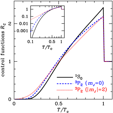
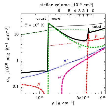
Figure 6: Left panel: Specific heat control functions for the ¹S₀ , ³P₂ ($m_{J}=0$), and ³P₂ ($|m_{J}|=2$) types of pairing listed in Sect. 3.1. The inset displays the same functions on a logarithmic scale. Right panel: Total and partial specific heats near the bottom of the crust and in the core of a neutron star at $T=10^{8}$ K as functions of density. The solid lines show the total $c_{\mathrm{v}}$, and the other lines show the contributions of electrons ($e^{-}$), neutrons ($n$), nuclei ($N$, in the crust), muons and protons ($\mu^{-}$ and $p$, in the core). Thin lines show results of a calculation with nucleons assumed to be unpaired, and thick lines take pairing into account. The top axis shows the volume contained inside a sphere with given $\rho$ for a 1.4 $M_{\odot}$ neutron star. The stellar structure and composition are adopted from the BSk21 model.

3.3 Superfluid effects on neutrino emission

The enormous impact of pairing on the cooling comes directly from the appearance of the energy gap $\Delta_{\mathrm{pair}}$ at the Fermi surface which leads to a suppression of all processes involving single particle excitations of the paired species. When $T\ll T_{\mathrm{c}}$ the suppression is of the order of $\mathrm{e}^{-\Delta_{\mathrm{pair}}/T}$ and hence dramatic. Its exact value depends on the details of the phase space involved in each specific process. In numerical calculations it is introduced as a control function. As well as for the heat capacity, for the neutrino emissivity one writes

$$Q_{\nu}=R_{\textrm{(pairing type)}}^{\textrm{(process type)}}Q_{\nu}^{(0)},$$ (19)

where $Q_{\nu}^{(0)}$ relates to the same process in the absence of pairing. These control functions (reduction factors) are available in the form of analytical fits, referenced in Table 1.

The superfluidity not only reduces the emissivity of the usual neutrino reactions but also initiates a specific “pair breaking and formation” (PBF) neutrino emission mechanism. The superfluid or superconducting condensate is in thermal equilibrium with the single particle (“broken pairs”) excitations and there is continuous formation and breaking of Cooper pairs. The formation of a Cooper pair liberates energy which can be taken away by a $\nu-\bar{\nu}$ pair (Flowers et al. 1976; Voskresensky and Senatorov 1987). This effect is most pronounced near the Fermi surface. When $T$ falls below $T_{\mathrm{c}}$, the neutrino emissivity produced by the Cooper pairing sharply increases. The PBF mechanism is sensitive to the model adopted for calculating the superfluid gaps in the baryon spectra: it is more important for lower gaps (weaker superfluid). Its emissivity is a sharp function of density and temperature. The main neutrino energy release takes place in the temperature interval between $\sim T_{\mathrm{c}}/5$ and $T_{\mathrm{c}}$. The control functions and the intensity of the Cooper-pair neutrino emission are available as analytical fits collected by Yakovlev et al. (2001) (see references therein for the original derivations), as indicated in Table 1 above.

Voskresensky and Senatorov (1987) noticed that the PBF mechanism is sensitive to the in-medium renormalization of the nucleon weak-interaction vertex due to strong interactions (cf. Sect. 2.6.3). Later this effect has been reexamined in many papers for different types of baryon pairing – see Leinson (2009, 2010) for modern results and a critical analysis of previous works. The net result is that the collective effects virtually kill down the PBF emission for the singlet pairing of nucleons, but leave this mechanism viable for the triplet pairing. Quantitatively, PBF emissivity estimated without in-medium effects (Yakovlev et al. 1999a) has to be multiplied by a small factor of $(p_{\mathrm{F}}/m^{*}c)^{2}$ in the ¹S₀ case, but by a moderate factor of $\approx 0.19$ in the ³P₂ case. This result lies at the basis of the “minimal cooling scenario” and the explanation of the observed fast cooling of the neutron star in the Cassiopeia A supernova remnant (see Sect. 6).

Superconductivity of protons may also induce another type of neutrino emission, electron-fluxoid scattering, in the presence of a strong magnetic field. It will be addressed in Sect. 4.3.

3.4 Superfluid effects on heat conduction

The effects of nucleon superfluidity on the heat transport in neutron stars were discussed qualitatively by Flowers and Itoh (1976, 1981). The thermal conductivity of electrons and muons was reconsidered by Gnedin and Yakovlev (1995) and later by Shternin and Yakovlev (2007), who obtained accurate analytical expressions valid for a wide class of models of superfluid and non-superfluid matter. Baiko et al. (2001a) reanalyzed the thermal conduction by neutrons, utilizing some new developments in the nucleon–nucleon interaction theory. The latter authors showed that the low-temperature behavior of the nucleon thermal conductivity is very sensitive to the relation between critical temperatures of neutrons and protons.

The lepton heat conduction in the core can also be affected by proton superconductivity, because superconductivity modifies the transverse polarization function and screening functions in neutron-star matter. These effects were studied by Shternin and Yakovlev (2007). These authors, as well as Baiko et al. (2001a), managed to describe the effects of superfluidity by analytical functions, which facilitate their inclusion in simulations of neutron-star thermal evolution (see Table 2).

In the presence of neutron superfluidity, there may be another channel of heat transport, the so-called convective counterflow of the normal component of matter with respect to the superfluid one. This mechanism is known to be quite effective in superfluid helium (e.g., Tilley and Tilley 1990), but in the context of neutron stars the situation is unclear and has not been studied in sufficient detail.

Heat can also be transported through the neutron star crust by collective modes of superfluid neutron matter, called superfluid phonons (Aguilera et al. 2009). At $\rho\approx 10^{12}-10^{14}$ g cm^-3 the conductivity due to superfluid phonons was estimated to be significantly larger than that due to lattice phonons and comparable to electron conductivity when $T\approx 10^{8}$ K. The authors found that this mode of heat conduction could limit the anisotropy of temperature distribution at the surface of highly magnetized neutron stars. However, new studies of the low-energy collective excitations in the inner crust of the neutron star (Chamel 2012; Chamel et al. 2013), including neutron band structure effects, show that there is a strong mixing between the Bogoliubov-Anderson bosons of the neutron superfluid and the longitudinal crystal lattice phonons. In addition, the speed of the transverse shear mode is greatly reduced as a large fraction of superfluid neutrons are entrained by nuclei. This results in an increased specific heat of the inner crust, but also in a decrease of the electron thermal conductivity. On the other hand, the entrainment of the unbound neutrons decreases the density of conduction neutrons, i.e., neutrons that are effectively free. The density of the conduction neutrons can be much smaller than the total density of unbound neutrons (Chamel 2012), which results in a decrease of the neutron thermal conductivity.

4 The effects of strong magnetic fields

4.1 Magnetic-field parameters

Convenient dimensionless parameters that characterize the magnetic field in a plasma are the ratios of the electron cyclotron energy $\hbar\omega_{\mathrm{c}}$ to the atomic unit of energy, electron rest energy, and temperature:

$$\gamma=\frac{\hbar^{3}B}{m_{e}^{2}ce^{3}}=\frac{B}{B_{0}},\qquad b=\frac{\hbar eB}{m_{e}^{2}c^{3}}=\frac{B}{B_{\mathrm{QED}}}\,,\qquad\zeta_{e}=\frac{\hbar\omega_{\mathrm{c}}}{T}=134.34\,\frac{B_{12}}{T_{6}}.$$ (20)

Here, $\omega_{\mathrm{c}}=eB/m_{e}c$ is the electron cyclotron frequency, $B_{0}=2.3505\times 10^{9}$ G is the atomic unit of magnetic field, $B_{\mathrm{QED}}=4.414\times 10^{13}$ G is the critical field in Quantum Electrodynamics (Schwinger 1988), and $B_{12}\equiv B/10^{12}$ G.

Motion of charged particles in a magnetic field is quantized in discrete Landau levels. In the non-relativistic theory, the energy of an electron in a magnetic field equals $N\hbar\omega_{\mathrm{c}}+m_{e}p_{z}^{2}/2$, where $p_{z}$ is the momentum component along $\bm{B}$, $N=n_{\mathrm{L}}+\frac{1}{2}\mp\frac{1}{2}$ characterizes a Landau level, the term $\mp\frac{1}{2}$ is the spin projection on the field, and $n_{\mathrm{L}}$ is the non-negative integer Landau number related to the quantization of the kinetic motion transverse to the field. In the relativistic theory (e.g., Sokolov and Ternov 1986), the kinetic energy $\epsilon$ of an electron at the Landau level $N$ depends on its longitudinal momentum $p_{z}$ as

$$\epsilon_{N}(p_{z})=c\,\left(m_{e}^{2}c^{2}+2\hbar\omega_{\mathrm{c}}m_{e}N+p_{z}^{2}\right)^{1/2}-m_{e}c^{2}.$$ (21)

The levels $N\geqslant 1$ are double-degenerate with respect to the spin projection $s$. Their splitting $\delta\epsilon$ due to the anomalous magnetic moment of the electron is negligible, because it is much smaller than $\hbar\omega_{\mathrm{c}}$ (e.g., Schwinger 1988; Suh and Mathews 2001):

$$\delta\epsilon\approx\frac{\alpha_{\mathrm{f}}}{2\pi}\times\left\{\begin{array}[]{l}\hbar\omega_{\mathrm{c}}\mbox{~{}at~{}}b\ll 1,\\ m_{e}c^{2}\,[\ln b-1.584]^{2}\mbox{~{}at~{}}b\gg 1,\end{array}\right.$$ (22)

where $\alpha_{\mathrm{f}}$ is the fine structure constant.

The Landau quantization becomes important when the electron cyclotron energy $\hbar\omega_{\mathrm{c}}$ is at least comparable to both the electron Fermi energy $\epsilon_{\mathrm{F}}$ and temperature $T$. If $\hbar\omega_{\mathrm{c}}$ is appreciably larger than both $\epsilon_{\mathrm{F}}$ and $T$, then the electrons reside on the ground Landau level, and the field is called strongly quantizing. The condition $\hbar\omega_{\mathrm{c}}>T$ is equivalent to $\zeta_{e}>1$. The condition $\hbar\omega_{\mathrm{c}}>\epsilon_{\mathrm{F},e}$ translates into $\rho<\rho_{B}$, where

$$\rho_{B}\approx 7045\,Y_{e}^{-1}\,B_{12}^{3/2}\text{ \mbox{g~{}cm${}^{-3}$}}.$$ (23)

In the opposite limit, where either $\zeta_{e}\ll 1$ or $\rho\gg\rho_{B}$, the field can be considered as nonquantizing.

For the ions, the cyclotron energy is $\hbar\omega_{\mathrm{ci}}=Z\,(m_{e}/m_{\mathrm{i}})\,\hbar\omega_{\mathrm{c}}$, and the Landau quantization is important when the parameter

$$\zeta_{\mathrm{i}}=\hbar\omega_{\mathrm{ci}}/T=0.0737\,(Z/A)\,B_{12}/T_{6}$$ (24)

is not small. The energy spectrum of an ion essentially differs from Eq. (21) because of the non-negligible anomalous magnetic moments. In the non-relativistic theory, the energy of an ion equals $\epsilon=(n_{\mathrm{L}}+\frac{1}{2})\hbar\omega_{\mathrm{ci}}+m_{\mathrm{i}}p_{z}^{2}/2+\frac{1}{4}\,g_{\mathrm{i}}\zeta_{\mathrm{i}}s_{\mathrm{i}},$ where $n_{\mathrm{L}}$ is the ion Landau number, $p_{z}$ is the longitudinal momentum, $g_{\mathrm{i}}$ is the $g$-factor ($g_{\mathrm{i}}=2$ in the Dirac theory, but, e.g., $g_{\mathrm{i}}=5.5857$ for the protons), and $s_{\mathrm{i}}$ is the integer quantum number corresponding to the spin projection on $\bm{B}$ in units of $\hbar/2$. If the ions are relativistic, the situation is much more complicated. For baryons with spin $\frac{1}{2}$ (e.g., protons) the energy spectrum was derived by Broderick et al. (2000).

4.2 Magnetic field effects on the equation of state and heat capacity

4.2.1 Magnetized core

A magnetic field can affect the thermodynamics of the Coulomb plasmas, if the Landau quantization is important, i.e., under the conditions that are quantified in Sect. 4.1. In particular, Eq. (23) can be recast into

$$B\gtrsim(3.8\times 10^{19}\mbox{ G})\,(Y_{e}n_{\mathrm{b}}/\mbox{fm}^{-3})^{2/3}.$$ (25)

We have $n_{\mathrm{b}}\sim 0.1$ fm^-3 near the crust-core interface, and $Y_{e}$ is typically several percent throughout the core. Therefore, the electron component of pressure in the core might be affected by the fields $B\gtrsim 10^{18}$ G.

One can easily generalize Eq. (25) for other fermions ($\mu$-mesons, nucleons) in the ideal-gas model. In this case, $Y_{e}$ should be replaced by the number of given particles per baryon, and the right-hand side should be multiplied by $m_{\mu}/m_{e}=206.77$ for muons and $\sim 10^{3}$ (of the order of nucleon-to-electron mass and electron-to-nucleon magnetic moment ratios) for protons and neutrons. Accordingly, the partial pressures of muons and nucleons in the core cannot be affected by any realistic ($B\lesssim\mbox{a few}\times 10^{18}$ G) magnetic field.

Broderick et al. (2000) developed elaborated models of matter in ultra-magnetized cores of neutron stars. They considered not only the ideal $npe\mu$ gas, but also interacting matter in the framework of the relativistic mean field (RMF) model. The magnetic field affects their EoS at $B\gtrsim 10^{18}$ G. As follows both from the estimates based on the virial theorem (Lai and Shapiro 1991) and from numerical hydrodynamic simulations (e.g., Frieben and Rezzolla 2012, and references therein), this field is close to the upper limit on $B$ for dynamically stable stellar configurations. The effect is even smaller when the magnetization of matter is included consistently in the EoS (Chatterjee et al. 2015). Therefore, it is unlikely that a magnetic modification of the EoS could be important in the cores of neutron stars.

4.2.2 Magnetized crust and ocean

At $B\gtrsim 10^{16}$ G, nuclear shell energies become comparable with the proton cyclotron energy. Thus the interaction of nucleon magnetic moments and proton orbital moments with magnetic field may cause appreciable modifications of nuclear shell energies. These modifications and their consequences for magnetars were studied by Kondratyev et al. (2001), who found large changes in the nuclear magic numbers under the influence of such magnetic fields. This effect may alter significantly the equilibrium chemical composition of a magnetar crust.

Muzikar et al. (1980) calculated the triplet-state neutron pairing in magnetized neutron-star cores. According to these calculations, magnetic fields $B\gtrsim 10^{16}$ G make the superfluidity with nodes at the Fermi surface energetically preferable to the usual superfluidity without nodes. Accordingly, the superfluid reduction factors for the heat capacity and neutrino emissivity (the control functions) may be different in ultra-strong fields.

Chamel et al. (2012) studied the impact of superstrong magnetic fields on the composition and EoS of the neutron star crust. In particular, they found that the neutron-drip pressure increases almost linearly by 40% from its zero-field value in the interval $10^{16}\mbox{ G}<B<5\times 10^{16}\mbox{ G}$. With further increase of the field strength, the drip pressure becomes directly proportional to $B$.

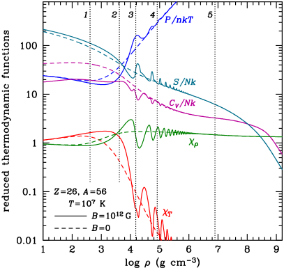
Figure 7: Left panel: Normalized pressure $P/n_{\mathrm{i}}T$; entropy $S$ and heat capacity $C_{V}$ per one ion, and logarithmic derivatives of pressure over density and temperature, $\chi_{\rho}$ and $\chi_{T}$, for a fully-ionized non-magnetic (dashed lines) and magnetized ($B=10^{12}$ G, solid lines) iron plasma at $T=10^{7}$ K. The vertical dotted lines mark the densities at which the electron Fermi temperature equals $T$ without (1) or with (2) the magnetic field, $\rho=\rho_{B}$ (3), $\Gamma_{\mathrm{C}}=\Gamma_{\mathrm{m}}$ (4), and $T_{\mathrm{p}}=T$ (5). (Figure 6 from Potekhin and Chabrier 2013, reproduced with the permission of ©ESO.) Right panel: Normalized thermal phonon contribution to the reduced heat capacity as a function of $\log_{10}(T/T_{\mathrm{p}})$ at different values of the ratio $\hbar\omega_{\mathrm{ci}}/T_{\mathrm{p}}$, marked near the curves.

Thus the ultra-strong fields $B\gtrsim 10^{16}$ G can affect various aspects of the physics of the inner crust in quite non-trivial way. Hereafter we will consider only fields $B\lesssim 10^{16}$ G. They can be quantizing in the outer crust of a neutron star, but not in the inner crust or the core. Analytical fitting formulae for the thermodynamic functions of the electron-ion plasmas in such fields, as well as a computer code that implements these fits, were published by Potekhin and Chabrier (2013). Such fields affect the electron part of thermodynamic functions in the outer envelopes only, as illustrated in the left panel of Fig. 7 in the case of fully-ionized iron at $T=10^{7}$ K and $B=10^{12}$ G (for illustration, the density range is extended to $\rho\lesssim 10^{5}$ neglecting the bound states that can be important in this $\rho$ – $T$ domain). We plot the principal thermodynamic quantities normalized per one ion as functions of density. For comparison we also show them in the absence of quantizing magnetic field. The vertical dotted lines marked by numbers separate different characteristic domains, consecutively entered with increasing density: onset of electron degeneracy at $B=0$ and at $B=10^{12}$ G, population of excited Landau levels ($\rho=\rho_{B}$), melting point with formation of a classical Coulomb crystal ($T_{\mathrm{m}}=T$), and onset of the quantum effects in the crystal ($T_{\mathrm{p}}=T$). The gradually decreasing oscillations correspond to consecutive filling of the electron Landau levels. The magnetic field $B=10^{12}$ G does not affect the ion contributions at this $T$.

The contributions of ions to the thermodynamic functions are affected by the magnetic field if the parameter $\zeta_{\mathrm{i}}$, defined by Eq. (24), is large. This may occur in a superstrong field of a magnetar. The right panel of Fig. 7 illustrates the effects of a superstrong field on $c_{\mathrm{v,i}}$ for the model of a harmonic Coulomb crystal (Baiko 2009). Here we plot the thermal phonon contribution to the heat capacity of the bcc Coulomb lattice calculated as the derivative $c_{\mathrm{v}}=T\partial S/\partial T$ of the fit to the phonon entropy $S$ given by Eq. (77) of Potekhin and Chabrier (2013). This approximation is more accurate for the heat capacity than the alternative approximation that provides exact fulfillment of the Maxwell relations (Eq. 80 of the same paper). The three steps on the curves in the right panel of Fig. 7 correspond to contributions of three branches of the phonon spectrum, which are affected differently by the quantizing magnetic field.

4.3 Magnetic field effects on neutrino emission

4.3.1 Magnetic Durca process

We have mentioned in Sect. 2.6.2 that the Durca reaction is the most efficient neutrino emission process, but it can only operate above a certain threshold density in the central parts of the cores of sufficiently massive neutron stars. Leinson and Pérez (1998) noted that a superstrong magnetic field can substantially weaken this requirement. An accurate study of this effect was performed by Baiko and Yakovlev (1999). They showed that the border between the open and closed Durca regimes is smeared out over some $B$-dependent scale and described this smearing by simple formulae. In practice this effect should be very important for neutron stars with $B\gtrsim 10^{16}$ G. At less extreme fields ($10^{14}\mbox{~{}G}\lesssim B\lesssim 10^{16}$ G) it is important for neutron stars whose mass happens to be close (within a few percent) to the Durca threshold mass. Baiko and Yakovlev (1999) also showed that a strong magnetic field has a non-trivial effect (oscillations of the reaction rate) in the permitted domain of the Durca reaction, but the latter effect, albeit interesting, appears to be unimportant.

4.3.2 Pair annihilation

The $e^{-}e^{+}$ pair annihilation process in strong magnetic fields was studied by Kaminker et al. (1992) and Kaminker and Yakovlev (1994). In a hot, non-degenerate plasma ($T\gtrsim 10^{10}$ K) only ultra-strong magnetic fields $B\gtrsim 10^{16}$ G can significantly affect the neutrino emissivity. Such fields can be quantizing in the $\rho-T$ domain where the pair emission dominates (see Fig. 3). They amplify $Q_{\mathrm{pair}}$ by increasing the number densities of electrons and positrons via very strong quantization of their motion. Lower fields may also influence $Q_{\mathrm{pair}}$ but less significantly. A field $B\sim 10^{14}$ G may quantize the motion of positrons at $T\lesssim 10^{9}$ K and increase the positron number density. In this way the presence of a strong magnetic fields greatly enhances $Q_{\mathrm{pair}}$ in a not too hot plasma. However, this enhancement usually takes place where the pair annihilation emissivity is much lower than the contribution from other neutrino reactions, and therefore it is unimportant for studies of neutron-star thermal evolution.

4.3.3 Synchrotron radiation

A relativistic electron propagating in the magnetic field can emit neutrinos because of its rotation around the magnetic field lines. This process is quite analogous to the usual synchrotron emission of photons. The calculation of the corresponding neutrino emissivity, $Q_{\mathrm{syn}}$, is similar to that of the pair annihilation process. It was studied, e.g., by Kaminker et al. (1992), Vidaurre et al. (1995), and Bezchastnov et al. (1997). In Fig. 8 we show the plot of $Q_{\mathrm{syn}}$ on the $\rho-T$ plane for two field strengths typical for magnetars, $B=10^{14}$ G and $10^{15}$ G. It is clear from this plot that the the synchrotron process can be dominant in the crust of magnetars in a large temperature range.

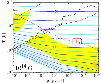
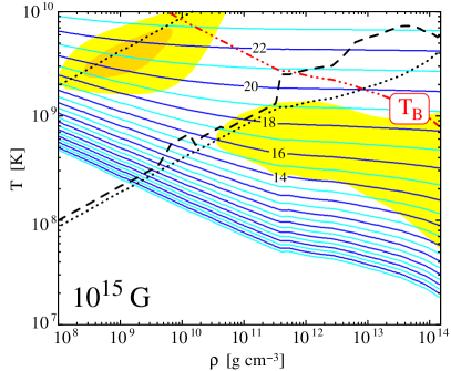
Figure 8: Neutrino emissivity in a magnetized crust from the synchrotron processes for two, uniform, magnetic field strengths of $10^{14}$ G (left panel) and $10^{15}$ G (right panel). The contour lines are labeled by the value of $\mathrm{log}_{10}[Q_{\nu}/(\mathrm{erg\,cm}^{-3}\,\mathrm{s}^{-1})]$. Regions where this process dominates over the ones shown in Fig. 3 are lightly shadowed (in yellow) and regions where it dominates by more than a factor of 10 are darkly shadowed (in orange). The two dotted lines show the dominance transitions between the three processes presented in Fig. 3. (Also indicated is the ion melting curve, dashed line.)

4.3.4 Electron-fluxoid scattering

The internal stellar magnetic field can be confined in the crust or be distributed over the entire star. In the latter case, a transition to a superconducting state in the course of stellar cooling is accompanied by a dramatic change in the spatial structure of the magnetic field. Initially homogeneous field splits into an ensemble of Abrikosov fluxoids – quantized magnetic flux tubes, which contain a superstrong magnetic field, embedded in the field-free superconducting medium. Neutrino synchrotron radiation is then modified and may be treated as neutrino pair emission due to scattering of electrons on the fluxoids. This mechanism was studied by Kaminker et al. (1997), who obtained an analytical fit to the corresponding neutrino emissivity (referenced in Table 1). The concentration of the field within the fluxoids amplifies the neutrino emissivity, compared to the usual synchrotron regime, when temperatures drops below the critical one for the protons, $T_{\mathrm{c}p}$. As long as $T$ is not much lower than $T_{\mathrm{c}p}$, the Cooper pairing mechanism remains much more powerful (unless $B\gg 10^{16}$ G, in which case the electron-fluxoid scattering may be more powerful at any $T$). At $T\ll T_{\mathrm{c}p}$, the electron-fluxoid scattering becomes the dominant neutrino emission mechanism for the neutron stars with strong and superstrong fields ($B\gtrsim 10^{12}$ G).

4.4 Magnetic field effects on heat conduction

4.4.1 Photon heat conduction

The thermal conductivity $\kappa$ is related to the opacity $\varkappa$ by the equation

$$\kappa=\frac{16\sigma_{\mathrm{SB}}T^{3}}{3\rho\varkappa},$$ (26)

where $\sigma_{\mathrm{SB}}$ is the Stefan-Boltzmann constant. The spectral radiative opacities for two normal polarization modes in strongly magnetized neutron-star photospheres are reviewed in Paper I. These opacities, $\varkappa_{\omega,j}(\theta_{B})$, where $j=1,2$ marks the extraordinary and ordinary polarization modes, depend on the angle $\theta_{B}$ between the wave vector and magnetic field. In the diffusion approximation, they combine into the effective opacities for the transport along ($\varkappa_{\omega,j}^{\|}$) and across ($\varkappa_{\omega,j}^{\perp}$) magnetic field according to

$$\left\{\begin{array}[]{c}(\varkappa_{\omega,j}^{\|})^{-1}\\ (\varkappa_{\omega,j}^{\perp})^{-1\rule{0.0pt}{6.02777pt}}\end{array}\right\}=\frac{3}{4}\int_{0}^{\pi}\left\{\begin{array}[]{c}2\cos^{2}\theta_{B}\\ \sin^{2}\theta_{B}\end{array}\right\}\frac{\sin\theta_{B}\,\mathrm{d}\theta_{B}}{\varkappa_{\omega,j}(\theta_{B})}\,.$$ (27)

The effective opacity for energy transport at angle $\theta$ to $\bm{B}$ in each polarization mode is given by $1/\bar{\varkappa}_{j}=\cos^{2}\theta/\bar{\varkappa}_{j}^{\|}+\sin^{2}\theta/\bar{\varkappa}_{j}^{\perp},$ where $\bar{\varkappa}$ is the Rosseland mean of $\varkappa_{\omega}$,

$$\frac{1}{\bar{\varkappa}_{j}}\equiv\int_{0}^{\infty}\frac{u(z)}{\varkappa_{\omega,j}}\mathrm{d}z,\quad u(z)=\frac{15}{4\pi^{4}}\frac{z^{4}\mathrm{e}^{z}}{(\mathrm{e}^{z}-1)^{2}},\quad z=\frac{\hbar\omega}{T}.$$ (28)

For fully ionized plasmas, the radiative opacities are contributed from the free-free absorption and Thomson scattering. Silant’ev and Yakovlev (1980) studied the Rosseland opacities for a non-polarized radiation in magnetized fully ionized plasmas

$$\varkappa_{\mathrm{r}}^{\|,\perp}=\left[1/\bar{\varkappa}_{1}^{\|,\perp}+1/\bar{\varkappa}_{2}^{\|,\perp}\right]^{-1}$$ (29)

using the Born approximation for the free-free contribution. Potekhin and Yakovlev (2001) obtained simple analytical fits for $\varkappa_{\mathrm{r}}^{\|,\perp}$, including a correction to the Born approximation, as functions of $\rho$, $T$, $Z$, $A$, and the magnetic-field parameter $\zeta_{e}$ defined by Eq. (20). Asymptotically, $\varkappa_{\mathrm{r}}\propto\zeta_{e}^{-2}$ at $\zeta_{e}\to\infty$.

At finite but large $\zeta_{e}$, the radiative opacities of fully ionized matter are strongly reduced. The reduction is $\sim 10$ times stronger for the Thomson scattering than for the free-free absorption. In deep, strongly magnetized photospheric layers the Thomson scattering dominates only if $T_{6}\gtrsim 10\,\rho^{2/7}\gtrsim 10\,B_{12}^{2/7}$; otherwise the free-free absorption prevails (Potekhin and Yakovlev 2001).

The outermost envelopes of neutron stars can be incompletely ionized in the cases of large $Z$ or $B$. The presence of bound species can strongly affect the radiative opacities and the spectrum of emitted radiation, as discussed in Paper I. However, the layers that are responsible for the heat flux from the interior of the neutron star to the surface, as a rule, lie at sufficiently large densities, where the plasma is fully ionized by pressure. Therefore the bound species are usually unimportant for the effective surface temperature of a neutron star.

4.4.2 Electron heat conduction

A non-quantizing magnetic field does not affect thermodynamic functions of the plasma. However, it does affect the electron heat conduction, if the Hall magnetization parameter

$$\omega_{\mathrm{g}}\tau\approx 1760\,\frac{B_{12}}{\sqrt{1+x_{\mathrm{r}}^{2}}}\,\frac{\tau}{10^{-16}\mathrm{~{}s}}$$ (30)

is not small. Here, $\omega_{\mathrm{g}}=\omega_{\mathrm{c}}/\sqrt{1+x_{\mathrm{r}}^{2}}$ is the electron gyrofrequency, and $\tau$ is the effective relaxation time. In a degenerate Coulomb plasma with a non-quantizing magnetic field, the main contribution is given by the electron-ion scattering according to Eq. (A.3). This regime has been studied by Yakovlev and Urpin (1980).

Electric and thermal currents induced in a magnetized plasma under the effect of an electric field $\bm{E}$, a weak gradient $\nabla\mu$ of the electron chemical potential, and a weak temperature gradient $\nabla T$ can be decomposed into conduction and magnetization components (e.g., Hernquist 1984). The latter ones relate to surface effects and must be subtracted. Let $\bm{j}_{e}$ and $\bm{j}_{T}$ be the conduction components of the electric and thermal current densities. They can be written as

$$\bm{j}_{e}=\hat{\sigma}\cdot\bm{E}^{\ast}-\hat{\alpha}\cdot\nabla T,\quad\bm{j}_{T}=T\hat{\alpha}\cdot\bm{E}^{\ast}-\hat{\tilde{\kappa}}\cdot\nabla T,$$ (31)

where $\bm{E}^{\ast}=\bm{E}+\nabla\mu/e$ is the electrochemical field. The symbols $\hat{\sigma}$, $\hat{\alpha}$, and $\hat{\tilde{\kappa}}$ denote second-rank tensors ($\hat{\sigma}$ is the conductivity tensor) which reduce to scalars at $B=0$. Equations (31) can be rewritten as

$$\bm{E}^{\ast}=\hat{R}\cdot\bm{j}_{e}-\hat{Q}\cdot\nabla T,\quad\bm{j}_{T}=T\hat{\alpha}\cdot\hat{R}\cdot\bm{j}_{e}-\hat{\kappa}\cdot\nabla T,$$ (32)

where $\hat{R}=\hat{\sigma}^{-1}$, $\hat{Q}=-\hat{R}\cdot\hat{\alpha}$, and $\hat{\kappa}=\hat{\tilde{\kappa}}+T\hat{\alpha}\cdot\hat{Q}$ are the tensors of specific resistance, thermopower, and thermal conductivity, respectively.

Electron heat and charge transport controlled by electron-ion collisions in quantizing magnetic fields of neutron stars was studied by Kaminker and Yakovlev (1981); Yakovlev (1984); Hernquist (1984); Potekhin (1996, 1999). The components of tensors $\hat{\sigma}$, $\hat{\alpha}$, and $\hat{\tilde{\kappa}}$ can be expressed as (Potekhin 1999)

$$\left\{\begin{array}[]{c}\sigma_{ij}\\ \alpha_{ij}\\ \tilde{\kappa}_{ij}\end{array}\right\}=\int_{0}^{\infty}\left\{\begin{array}[]{c}e^{2}\\ e{(\mu-\epsilon)/T}\\ {(\mu-\epsilon)^{2}/T}\end{array}\right\}\frac{\mathcal{N}_{B}(\epsilon)}{m_{e}+\epsilon/c^{2}}\,\tau_{ij}(\epsilon)\left[-\frac{\partial}{\partial\epsilon}\frac{1}{\mathrm{e}^{(\epsilon-\mu)/T}+1}\right]\mathrm{d}\epsilon,$$ (33)

where

$$\mathcal{N}_{B}(\epsilon)=\frac{1}{2\pi^{2}a_{\mathrm{m}}^{2}\hbar}\sum_{N=0}^{N_{\mathrm{max}}}(2-\delta_{N,0})|p_{z}|,$$ (34)

$N_{\mathrm{max}}$ is the maximum Landau number for a given electron energy $\epsilon$, and $|p_{z}|$ depends on $\epsilon$ and $N$ according to Eq. (21). In a non-quantizing magnetic field, i.e., at $N_{\mathrm{max}}\gg 1$, the sum can be replaced by the integral, which gives $\mathcal{N}_{B}(\epsilon)=(p/\hbar)^{3}/3\pi^{2}$, where $p$ is the momentum that corresponds to the energy $\epsilon$. The functions $\tau_{ij}(\epsilon)$ play role of relaxation times for the components of tensors $\hat{\sigma}$, $\hat{\alpha}$, and $\hat{\tilde{\kappa}}$, determined by electron scattering. In general, they differ from the mean free time $\tau_{e\mathrm{i}}(\epsilon)=1/\nu_{e\mathrm{i}}(\epsilon)$ between scattering events for an electron with energy $\epsilon$. Because of the symmetry properties of the tensors $\hat{\sigma}$, $\hat{\alpha}$, and $\hat{\tilde{\kappa}}$, in the coordinate frame with $z$ axis directed along $\bm{B}$, there are only three different non-zero components of $\tau_{ij}$: $\tau_{zz}$ related to longitudinal currents, $\tau_{xx}=\tau_{yy}$ related to transverse currents, and $\tau_{xy}=-\tau_{yx}$ related to the Hall currents.

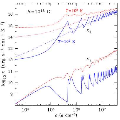
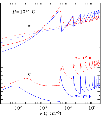
Figure 9: Electron thermal conductivities along (upper curves) and across (lower curves) magnetic field $B=10^{13}$ G (left panel) and $10^{15}$ G (right panel) as functions of mass density at temperatures $T=10^{7}$ K (solid lines) and $10^{8}$ K (dot-dashed lines). For comparison, the non-magnetic thermal conductivities are shown by dotted lines.

In a quantizing magnetic field, there are two different effective mean-free times $\tau_{\|}(\epsilon)$ and $\tau_{\perp}(\epsilon)$, corresponding to electron transport parallel and perpendicular to $\bm{B}$. In this case, the classical expressions (e.g., Yakovlev and Urpin 1980) are recovered:

$$\tau_{zz}=\tau_{\|},\quad\tau_{xx}=\frac{\tau_{\perp}}{1+(\omega_{\mathrm{g}}\tau_{\perp})^{2}},\quad\tau_{yx}=\frac{\omega_{\mathrm{g}}\tau_{\perp}^{2}}{1+(\omega_{\mathrm{g}}\tau_{\perp})^{2}}.$$ (35)

It is convenient to keep using Eq. (A.3) for $\tau_{\|}$ and $\tau_{\perp}$, but with different Coulomb logarithms $\Lambda_{\|}(\epsilon)$ and $\Lambda_{\perp}(\epsilon)$. Potekhin (1999) calculated these Coulomb logarithms and fitted them by analytic expressions. Their Fortran implementation is available at http://www.ioffe.ru/astro/conduct/. In the limit of non-quantizing magnetic field, $\tau_{\|}=\tau_{\perp}=\tau_{e\mathrm{i}}(\epsilon)$ is given by Eq. (A.3) with $\epsilon=\mu$.

When the electrons are strongly degenerate, the derivative in the square brackets in Eq. (33) is sharply peaked. Then Eq. (33) gives

$$\sigma_{ij}\approx\frac{e^{2}c^{2}n_{e}}{\mu}\,\tau_{ij}(\mu),\qquad\kappa_{ij}\approx\tilde{\kappa}_{ij}\approx\frac{\pi^{2}T}{3e^{2}}\,\sigma_{ij}.$$ (36)

The latter relation is the Wiedemann-Franz law generalized to the magnetic case. On the other hand, Eq. (33) satisfactorily describes the conductivities in general, including the opposite case of weakly degenerate electrons.

Figure 9 illustrates the $\rho$-dependence of the thermal conductivities along ($\kappa_{\|}$) and across ($\kappa_{\perp}$) the magnetic field. The first, most significant peak at $\kappa_{\|}$ is related to the filling of the first Landau level by the electrons at $\rho\sim\rho_{B}$. The other peaks correspond to consecutive filling of higher Landau levels.

5 Thermal structure of neutron stars

5.1 Blanketing envelopes

The very different thermal relaxation timescales of the envelope and the crust of a neutron stars makes computationally expensive to perform cooling simulations in a numerical grid that comprises both regions. Radiative equilibrium is established in the low-density region much faster than the crust evolves, so that the envelope reaches a stationary state on shorter timescales. Thus, the usual approach is to use results of stationary envelope models to obtain a relation between the photon flux $F_{\mathrm{ph}}$ radiated from the surface and the flux $F_{\mathrm{b}}$ and temperature $T_{\mathrm{b}}$ at the crust/envelope boundary, $\rho=\rho_{\mathrm{b}}$. This relation supplements the evolution equations for the interior [Eq. (4)] as an outer boundary condition.

The boundary density $\rho_{\mathrm{b}}$ is chosen as a trade-off between two requirements: first, that the thermal relaxation time of the layer with $\rho<\rho_{\mathrm{b}}$ is short compared to the characteristic variability time of the studied thermal radiation, which favors smaller $\rho_{\mathrm{b}}$, and second, that $T$ does not strongly vary at $\rho>\rho_{\mathrm{b}}$, which favors larger $\rho_{\mathrm{b}}$. For weakly magnetized, isolated cooling neutron stars, $\rho_{\mathrm{b}}$ is usually set at $10^{10}$ g cm^-3 (Gudmundsson et al. 1983), but in general it varies from $10^{8}$ g cm^-3 for neutron stars with rapid variations of thermal emission (Shternin et al. 2007) to $\rho_{\mathrm{drip}}$ for relatively hot and strongly magnetized neutron stars (Potekhin et al. 2003).

At every $T_{\mathrm{b}}$, $F_{\mathrm{ph}}$ or, equivalently, the effective surface temperature $T_{\mathrm{s}}$, depends on the properties of the heat-blanketing envelopes. In the absence of neutrino energy losses in the envelope (that is the case for most cooling neutron stars, except for the hottest ones), the flux $F_{\mathrm{ph}}$ at the surface is equal to the flux $F_{\mathrm{b}}$ at the inner boundary of the blanketing envelope. Then it is sufficient to know the $T_{\mathrm{b}}$ – $T_{\mathrm{s}}$ relation for cooling simulations.

Gudmundsson et al. (1983) carried out a comprehensive study of the thermal structure of the non-magnetized blanketing envelopes composed of iron, using the best physics input available at that time. They considered the envelopes with $\log_{10}T_{\mathrm{s}}$[K]$\geq 5.25$ (there were no reliable calculation of the thermal conductivities for lower temperatures) and fitted the numerical solutions by a remarkably simple formula

$$T_{\mathrm{b}}=1.288\times 10^{8}\,(T_{\mathrm{s6}}^{4}/g_{14})^{0.455}~{}~{}\mathrm{K},$$ (37)

where $T_{\mathrm{s6}}=T_{\mathrm{s}}/10^{6}$ K. An analytical derivation of a similar expression was given by Ventura and Potekhin (2001). A more accurate but less simple fit was constructed by Potekhin et al. (1997).

The $T_{\mathrm{b}}$ – $T_{\mathrm{s}}$ relation is mainly regulated by the thermal conductivity in the “sensitivity strip” (Gudmundsson et al. 1983) that plays the role of a “bottleneck” for the heat leakage. Its position lies around the line where $\kappa_{\mathrm{r}}=\kappa_{e}$ (as a rule, around $\rho\sim 10^{5}$ – $10^{7}$ g cm^-3 for $B=0$) and depends on the stellar structure, the boundary temperature $T_{\mathrm{b}}$, the magnetic field $\bm{B}$ in the vicinity of the given surface point, and the chemical composition of the envelope. Since the magnetic field hampers heat transport across $\bm{B}$, the depth of the sensitivity strip can be different at different places of a star with a strong magnetic field: it lies deeper at the places where the magnetic field lines are parallel to the surface (Ventura and Potekhin 2001).

The blanketing envelopes are more transparent to the heat flux, if they are composed of light chemical elements. This effect was studied in detail by Potekhin et al. (1997) for non-magnetic envelopes and by Potekhin et al. (2003) for strongly magnetized envelopes. The effect is related to the $Z$-dependence of the collision frequencies $\nu_{e\mathrm{i}}$. The higher is $Z$, the larger is $\nu_{e\mathrm{i}}$ and the lower is the conductivity. A temperature variation by a factor of 30 can change the thermal conductivity of iron plasma less than altering the chemical composition from Fe to He at a fixed $T$. This effect has important consequences for the relationship between the surface and internal temperatures of neutron stars. For example, combined effects of strong magnetic fields and light-element composition simplify the interpretation of magnetars: these effects allow one to interpret observations assuming less extreme (therefore, more realistic) heating in the crust (Kaminker et al. 2009; Pons et al. 2009; Viganò et al. 2013).

The envelope is thin (its depth $z_{\mathrm{b}}\sim 100$ m, if $\rho_{\mathrm{b}}=10^{10}$ g cm^-3) and contains a tiny fraction of the neutron-star mass ($\sim 10^{-7}$, if $\rho_{\mathrm{b}}=10^{10}$ g cm^-3). Therefore one can neglect the variation of the gravitational acceleration in this layer. Neglecting also the non-uniformity of the energy flux through the envelope due to the neutrino emission (which is small, if the neutron star is not too hot, as we discuss below) and the variation of the temperature $T_{\mathrm{s}}$ over the surface (which varies on larger length scales than $z_{\mathrm{b}}$), one can obtain, instead of Eq. (4), the much simpler thermal structure equation (Gudmundsson et al. 1983; Van Riper 1988)

$$\frac{{\rm d}\ln T}{{\rm d}\ln P}=\frac{3}{16}\,\frac{P\varkappa}{g}\,\frac{T_{\mathrm{s}}^{4}}{T^{4}},$$ (38)

where$\varkappa$ is the total opacity, related to the conductivity $\kappa$ via Eq. (26).

The assumption of a constant flux, however, breaks down for magnetars, most of which have atypically high effective temperatures. In this case one should solve the complete set of equations, taking neutrino emission and heat sources into account. The neutrino emission from the crust limits the effective surface temperature of a cooling neutron star (Potekhin et al. 2007; cf. Fig. 11 below). This very same effect is what limits the maximum flux in the few days of a magnetar outburst (Pons and Rea 2012). In addition, for magnetars one must go beyond the plane-parallel approximation (see Sect. 5.3)

5.2 The effects of strong magnetic fields

As seen from Eqs. (30) and (A.3), the Hall magnetization parameter is large in the outer neutron-star envelope at $B\gtrsim 10^{11}$ G. Moreover, the magnetic field can be strongly quantizing in the outermost part of the envelope. In this case the magnetic field can greatly affect the heat conduction and the thermal structure.

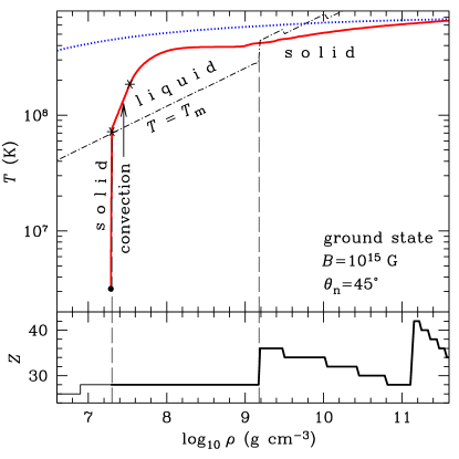
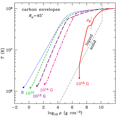
Figure 10: Thermal structure of blanketing envelopes with different magnetic fields. Left panel: temperature profile (solid line in the left top panel) for an envelope with ground-state composition, with $Z$ values shown in the bottom left panel, for a neutron star with surface gravity $g=1.6\times 10^{14}$ cm s^-2, magnetic field $B=10^{15}$ G directed at $45^{\circ}$ to the surface, and internal temperature $T_{\mathrm{b}}=6.7\times 10^{8}$ K, which yields the effective surface temperature $T_{\mathrm{s}}=3.16\times 10^{6}$ K. The dot-dashed line is the melting line. The asterisks confine the part of the profile where heat is carried by convection. For comparison, the non-magnetic profile with the same $T_{\mathrm{b}}$ is shown by dotted line. Right panel: temperature profiles for carbon blanketing envelopes for a neutron star with $g=1.4\times 10^{14}$ cm s^-2, $T_{\mathrm{b}}=10^{8}$ K, and magnetic fields $B=0$ (dotted line), $10^{12}$ G (short dashes), $10^{13}$ G (long dashes), $10^{14}$ G (alternating short and long dashes), and $10^{15}$ G (solid line). The vertical segment of the dot-dashed melting line corresponds to the maximum density for carbon, according to the thermonuclear stability criterion of Potekhin and Chabrier (2012), where carbon gives way to heavier chemical elements, which form a crystal. The heavy dots mark the position of the radiative surface, where $T$ equals the effective surface temperature $T_{\mathrm{s}}$.

Figure 10 shows examples of the temperature profiles in the envelopes. The left panel is a recast of Fig. 8 from Potekhin and Chabrier (2013). Here we show a profile of an ultra-magnetized neutron star, with $B=10^{15}$ G, and with relatively high surface temperature, $\log_{10}T_{\mathrm{s}}{}(K)=6.5$, which is similar to the values evaluated for some magnetars. In this case, thermal photons are radiated from a solid surface, with high mass density $\rho=2\times 10^{7}$ g cm^-3 just below the surface. The temperature quickly grows at the solid surface and reaches the melting point at the depth $z\approx 7$ cm. Thus, at the given conditions, the liquid ocean of a magnetar turns out to be covered by a thin layer of “ice” (solid substance). We treat the solid crust as immobile, but the liquid layer below the “ice” is convective up to the depth $z\sim 1$ m. The change of the heat-transport mechanism from conduction to convection causes the break of the temperature profile at the melting point in Fig. 10. We underline that this treatment is only an approximation. In reality, the superadiabatic growth of temperature can lead to a hydrostatic instability of the shell of “ice” and eventually to its cracking and fragmentation into turning-up “ice floes”. Potekhin and Chabrier (2013) speculated that such events may result in variations of thermal luminosity of magnetars. The temperature profile flattens with density increase, and the Coulomb plasma freezes again at the interface between the layers of ⁶⁶Ni and ⁸⁶Kr at $\rho=1.5\times 10^{9}$ g cm^-3.

For comparison, we also show the thermal profile without the magnetic field. It is smooth. There is neither magnetic condensation nor convection. In this case, the spectrum is formed in the gaseous atmosphere at much lower density beyond the frame of the left panel.

In the right panel of Fig. 10 we compare temperature profiles for a neutron star with internal temperature $10^{8}$ K and heat blanketing envelopes made of carbon, endowed with different magnetic fields. For the field strengths up to $10^{14}$ G, the radiation is formed in the gaseous atmosphere, whose density gradually becomes larger with increasing magnetic fields, due to the reduction of the effective opacities discussed in Sect. 4.4.1. The temperature profiles are rather smooth. The blanketing envelopes are liquid at this temperature. At the largest field strength $B=10^{15}$ G, however, the situation is qualitatively different. As well as in the case of the hotter ultra-magnetized ground-state envelope in the left panel, the heat is radiated from the condensed solid surface. Below the surface, at density $10^{7}$ g cm^-3, the temperature quickly grows, which causes melting of the Coulomb crystal with formation of a Coulomb liquid beneath the solid surface. With further density increase, the profile suffers a break at $\rho_{B}\approx 4.5\times 10^{8}$ g cm^-3 [Eq. (23)], where the electrons start to populate the first excited Landau level, which is associated with the peak of the thermal conductivity around $\rho_{B}$ (cf. Fig. 9).

As we have seen in Sect. 4.4, the conduction is strongly anisotropic in these conditions. Therefore the effective local surface temperature $T_{\mathrm{s}}$ is non-uniform and depends on the magnetic field geometry. Figure 11 shows examples of the relations between $T_{\mathrm{s}}$ and $T_{\mathrm{b}}$ deep in the crust for the magnetic fields $B=10^{12}$ G and $10^{15}$ G perpendicular and parallel to the radial direction. The relations obtained in the 1D approximation (Potekhin et al. 2007) with and without allowance for neutrino emission are plotted by the solid and dotted lines, respectively. We see that at $T_{\mathrm{b}}\lesssim 10^{8}$ K the neutrino emission does not affect $T_{\mathrm{s}}$. At higher $T_{\mathrm{b}}\gtrsim 10^{9}$ K, in contrast, this emission is crucial: if $Q_{\nu}=0$, then $T_{\mathrm{s}}$ continues to grow up with increasing $T_{\mathrm{b}}$, whereas with realistic $Q_{\nu}$ the surface temperature tends to a constant limit, which depends on $\bm{B}$. In most cases this limit is reached when $T_{\mathrm{b}}\sim 10^{9}$ K.

Since the distribution of $T_{\mathrm{s}}$ over the neutron-star surface is non-uniform in strong magnetic fields, it is convenient to introduce the overall effective temperature of the star, $T_{\mathrm{eff}}$, defined by

$$4\pi\sigma_{\mathrm{SB}}R^{2}T_{\mathrm{eff}}^{4}=L_{\mathrm{ph}}=\int F_{\mathrm{ph}}\,\mathrm{d}\Sigma=\sigma_{\mathrm{SB}}\int T_{\mathrm{s}}^{4}\,\mathrm{d}\Sigma,$$ (39)

where $F_{\mathrm{ph}}$ is the local flux density and $\mathrm{d}\Sigma$ is the surface element. The quantities $T_{\mathrm{s}}$, $T_{\mathrm{eff}}$, and $L_{\mathrm{ph}}$ refer to a local reference frame at the neutron-star surface. The redshifted (“apparent”) quantities as detected by a distant observer are (Thorne 1977):

$$R^{\infty}=R/\sqrt{1-r_{g}/R},\qquad T_{\mathrm{eff}}^{\infty}=T_{\mathrm{eff}}\,\sqrt{1-r_{g}/R},\qquad L_{\mathrm{ph}}^{\infty}=(1-r_{g}/R)\,L_{\mathrm{ph}}.$$ (40)

The effects of quantizing magnetic fields on the thermal structure of neutron-star envelopes were first studied by Hernquist (1985) and somewhat later by Van Riper (1988) and Schaaf (1990), using the 1D approximation. Van Riper (1988) considered a neutron star with a constant radial magnetic field. In this model, the quantum enhancement of conductivity at $\rho$ near $\rho_{B}$, seen in Fig. 9, results in an overall enhancement of the neutron-star photon luminosity $L_{\mathrm{ph}}$ at a fixed $T_{\mathrm{b}}$. Consequently, Van Riper (1991) found a strong effect of the magnetic field $B\sim 10^{13}$ G on the neutron-star cooling. However, Shibanov and Yakovlev (1996) showed that, for the dipole field distribution, the effects of suppression of the heat conduction across $\bm{B}$ at the loci of nearly tangential field can compensate or even overpower the effect of the conductivity increase near the normal direction of the field lines. This conclusion confirmed the earlier conjectures of Hernquist (1985) and Schaaf (1990). In the 2000s, detailed studies of the $T_{\mathrm{b}}$ – $T_{\mathrm{s}}$ relation in strong magnetic fields were performed for iron envelopes (Potekhin and Yakovlev 2001) and accreted envelopes composed of light elements (Potekhin et al. 2003), as well as for the large-scale (dipole) and small-scale (stochastic) surface magnetic fields (Potekhin et al. 2005). These studies confirmed the conclusions of Shibanov and Yakovlev (1996), but showed that in superstrong fields $B\gtrsim 10^{14}$ G the quantum enhancement of the conductivity and the corresponding increase of $T_{\mathrm{s}}$ at the places where $\bm{B}$ is nearly radial overpowers the decrease in the regions of nearly tangential field lines, so that $T_{\mathrm{eff}}$ at a given $T_{\mathrm{b}}$ increases. However, this may not be the case in the configurations where the field is nearly tangential over a significant portion of the stellar surface as, e.g., in the case of a superstrong toroidal field (Pérez-Azorin et al. 2006; Page et al. 2007).

5.3 Non-radial heat transport

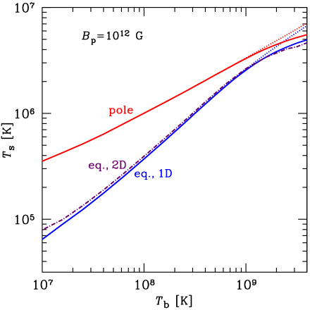
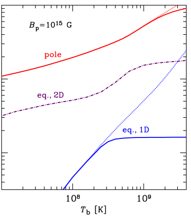
Figure 11: Local effective surface temperature $T_{\mathrm{s}}$ as function of the temperature $T_{\mathrm{b}}$ at the bottom of a non-accreted heat blanketing envelope with $\rho_{\mathrm{b}}=10^{10}$ g cm^-3 for a neutron star with mass $M=1.4\,M_{\odot}$, radius $R=12.6$ km, and the dipole magnetic field with polar strength $B_{\mathrm{p}}=10^{12}$ G (left panel) and $10^{15}$ G (right panel). Solid lines – 1D calculation with allowance for neutrino emission from the crust, dotted lines – neutrino emission is neglected. The upper dotted or solid curve shows $T_{\mathrm{s}}$ at the magnetic pole, and the lower curve curve shows $T_{\mathrm{s}}$ at the equator. The dot-dashed curve shows the result of a full 2D calculation for $T_{\mathrm{s}}$ at the magnetic equator.

As we mentioned in Sect. 5.1, in the case where $\bm{B}$ is nearly parallel to the surface, the 1D approximation fails, because the heat is transported along the field lines from the hotter surface regions outside the considered patch of the surface. Therefore the 1D approximation overestimates the heat blanketing effect in regions with nearly tangential magnetic fields. For a dipole field geometry it is an equatorial region , whose width can be estimated as $\sim 10$% of the radius (Potekhin et al. 2007). Since these regions are also the coldest ones, their contribution to the total flux is negligible. Then the 1D approximation well reproduces the integrated observed flux. However, it is not the case for magnetars, which may have a complex field geometry. A 2D treatment shows that the 1D approach is reliable in the regions where magnetic field lines make a substantial angle to the surface (Kaminker et al. 2012, 2014), but it predicts too low surface temperatures when the tangential magnetic field dominates (see Section 3 in Pons et al. 2009). Therefore for magnetars one must go beyond the 1D approximation. Complex field configurations which lack cylindrical symmetry may require the full 3D treatment, which has not been done yet.

In Fig. 11 we show results of 2D calculations in the dipole field geometry, compared with the 1D results. In this case, we see a substantial increase of $T_{\mathrm{s}}$ at the magnetic equator. This effect is especially pronounced for the superstrong field on the right panel. In Appendix B. we give an analytical approximation to the $T_{\mathrm{b}}$ – $T_{\mathrm{s}}$ relation in the case of a strong magnetic field, including the effects of neutrino emission from the crust.

6 Thermal evolution of neutron stars

6.1 Cooling scenarios

Several tens of seconds after birth, the protoneutron-neutron star has lost its excess lepton content, it has finished its residual contraction and becomes transparent to neutrino emission (Burrows and Lattimer 1986; Pons et al. 1999; Roberts 2012). Soon after that, the temperature distribution in the highly conductive stellar core reaches equilibrium, which is preserved thereafter throughout the star lifetime (except during short periods after catastrophic phase transitions in the core postulated by certain hypothetical models).

In the initial cooling stages, the stellar crust is hotter than the core, which is rapidly cooled down by the copious neutrino emission. The cooling wave reaches the surface within 10 –100 years; thereafter, the star cools down in the quasistationary regime. Since all currently observed neutron stars are at least several centuries old, they should be in the state of quasistationary cooling, except during transient events with significant energy release in the crust or the ocean discussed below.

Cooling in the quasistationary regime goes through two major stages. The first, neutrino cooling stage lasts $\sim 10^{5}$ years. During this period, the core cools mostly via neutrino emission. The second, photon cooling stage begins when the low temperature of the core makes the neutrino energy losses smaller than the losses due to electromagnetic radiation from the surface (see, e.g., Yakovlev and Pethick 2004, and references therein). This occurs at the age of $\approx 10^{5}$ years, depending on the particular stellar model and local conditions.

A theoretical cooling curve of an isolated neutron star, which shows the photon luminosity of the star $L_{\mathrm{ph}}$ or its temperature as a function of age $t$, depends on the stellar mass $M$, on the model of superdense matter in the core, which in particular, determines the intensity of neutrino emission and the EoS (and hence the stellar radius $R$), and on the properties of the envelopes. The latter include the thermal conductivity, which determines $L_{\mathrm{ph}}$ at a given internal stellar temperature, the neutrino luminosity $Q_{\nu}$ in the stellar crust, and the intensity of heating sources $H$. For highly magnetized neutron stars, the cooling curve also depends on the magnetic field $\bm{B}$ (on both its strength and configuration), since it affects the microphysics (conductivities, EoS, specific heat, etc.). Therefore, in general, the thermal evolution equations (4) should be supplemented by the equations that describe evolution of the magnetic field and electric currents in the star, which leads to the thermomagnetic evolution scenarios (see the review by Mereghetti et al. 2015 and references therein).

By comparing theoretical cooling curves with the observed $L_{\mathrm{ph}}$ and $t$ of isolated neutron stars, one can eventually place bounds on the theoretical models of superdense matter. At contrast, most neutron stars in binary systems have an additional source of energy (accretion) and an additional source of X-ray radiation (accretion disk), often much more powerful than the surface thermal emission. For this reason, they cannot be used to test cooling models.

The theoretical cooling scenarios are currently divided into two main classes: “minimal cooling” and “enhanced cooling”. The enhanced cooling implies fast neutrino emission processes, such as Durca reactions (Sect. 2.6.2), whereas the minimal cooling does not include such processes, but may be enhanced at the epoch of the onset of the baryon superfluidity via the PBF neutrino emission mechanism (Sect. 3.3), which helps to explain the variety of the observed surface temperatures of cooling neutron stars (Gusakov et al. 2004; Page et al. 2004). A spectacular example is the neutron star CXO J232327.9+584842 in the Cassiopeia A supernova remnant, dubbed Cas A NS, which shows an unexpectedly appreciable temperature decline during several years (Heinke and Ho 2010; Elshamouty et al. 2013) (but see Posselt et al. 2013 for tentative alternative interpretations of the observations). This decline can be comfortably explained by the PBF emission (Page et al. 2011; Shternin et al. 2011; see also Ho et al. 2015 for a recent analysis including modern observational data).

6.2 Heating mechanisms

In the course of their evolution, some regions of neutron stars may not only cool but also heat up by different mechanisms. For instance, the polar cap of a pulsar can be heated by a stream of electrons or positrons moving along open field lines from the magnetosphere. The temperature of “hot spots” produced by this additional heat deposited onto the stellar surface may be much higher than the average temperature of the star (e.g., Greenstein and Hartke 1983). Non-uniform heating processes occur also during accretion episodes (e.g., Inogamov and Sunyaev 2010). The hot polar caps emit much more intense X-rays than the remaining surface; as a result, such neutron stars become X-ray pulsars. Pulsed X-ray radiation is also observed from thermonuclear explosions of accreted matter at the surface of a rotating neutron star (see, e.g., review by Strohmayer and Bildsten 2006).

On the other hand, a neutron star may also be heated from inside, for example due to dissipation of a strong magnetic field (e.g., Miralles, Urpin and Konenkov 1998; Urpin and Konenkov 2008; Pons et al. 2009). It has been suggested that dissipation of superstrong magnetic fields may be responsible for the high effective temperatures of magnetars (Thompson 2001; see Mereghetti et al. 2015, for a review). Noticeable liberation of energy in the crust may also occur during starquakes (Haensel et al. 1990; Franco et al. 2000; Perna and Pons 2011). Two heating processes related to the secular spin-down of the star have also been proposed: vortex creep, the dissipative motion of superfluid vortices through the neutron star crust (Alpar et al. 1984), and rotochemical heating, the energy released by non-equilibrium beta decays due to the slow contraction of the neutron star as its centrifugal force decreases (Reisenegger 1995). Gonzalez and Reisenegger (2010) performed a comparative study of several heating mechanisms and found that the rotochemical heating and vortex creep can be most important for classical and millisecond pulsars. Both processes, albeit model-dependent, can keep millisecond pulsars at a surface temperature $T_{\mathrm{eff}}\sim 10^{5}$ K.

Another class of neutron stars undergoing heating episodes are quasipermanent transients, i.e., those soft X-ray transients (SXTs) whose active and quiescent periods last a few years or longer. During high-state accretion episodes, compression of the crust under the weight of newly accreted matter results in deep crustal heating, driven by exothermic nuclear transformations (Haensel and Zdunik 1990, 2008). For a given neutron star model, one can calculate the heating curve, that is the dependence of the equilibrium accretion-free $T_{\mathrm{eff}}$ on the accretion rate averaged over a large period of time. There is a close correspondence between the theory of thermal states of transiently accreting neutron stars and the theory of neutron star cooling (Yakovlev et al. 2003). Comparing the heating curves with a measured equilibrium $T_{\mathrm{eff}}$ value, one can constrain parameters connected to properties of dense matter (Yakovlev et al. 2004; Levenfish and Haensel 2007; Ho 2011). Wijnands et al. (2013) discuss prospects of application of such analysis to various classes of X-ray transients. The SXTs that have recently turned into quiescence allow one to probe the state of the neutron-star crust with the observed decline of $T_{\mathrm{eff}}$. Brown et al. (1998) suggested that during this decline the radiation is fed by the heat that was deposited in the crust in the preceding active period. Such cooling is independent of the details of the star structure and composition and therefore its analysis directly yields information on the physics of the crust. Observations of several sources can be interpreted in terms of this hypothesis and yield constraints to the heat conductivity in the neutron-star crust, as, e.g., for KS 1731–260 (Shternin et al. 2007; Brown and Cumming 2009), XTE J1701–462 (Fridriksson et al. 2011; Page and Reddy 2013), EXO 0748–676 (Turlione et al. 2015). The conductivity proves to be rather high, which means that the crust has a regular crystalline (not amorphous) structure. On the other hand, there are similar objects which display variations of thermal flux that do not conform to the thermal-relaxation scenario, which may be caused by a residual slow accretion on the neutron star in quiescence (Rutledge et al. 2002; Coti Zelati et al. 2014; Turlione et al. 2015).

6.3 Thermal luminosities of isolated neutron stars

The inferred effective temperature depends on the choice of the emission model (blackbody vs. atmosphere models, composition, condensed surface, etc. – see Paper I), which typically results in variation of $T_{\mathrm{eff}}$ by a factor $\approx 2-3$, and it has even larger theoretical uncertainties in the case of strong magnetic fields. In addition, photoelectric absorption in the interstellar medium further constitutes a source of error in temperature measurements, since the value of the hydrogen column density $N_{\mathrm{H}}$ is correlated to the temperature value obtained in spectral fits. Different choices for the absorption model and the metal abundances can also yield different results for the temperature. Last, in the case of data with few photons and/or strong absorption features, the temperature is poorly constrained by the fit, adding a large statistical error to the systematic one.

Table 3: Cooling neutron stars. $t_{\mathrm{c}}$ is the characteristic age, $t_{\mathrm{k}}$ is the kinematic age, and $f_{\mathrm{X}}$ is the unabsorbed flux in the 1–10 keV band. The range of luminosities $L$ includes both statistical and distance errors; for strongly absorbed sources (i.e., most magnetars) a minimum arbitrary factor of $50\%$ uncertainty is assumed to account for systematical model-dependent uncertainties. Data have been taken from Viganò et al. (2013) (see references therein and the online catalog in http://www.neutronstarcooling.info.)

Source	$\log_{10}(t_{\mathrm{c}})$	$\log_{10}(t_{\mathrm{k}})$	$\log_{10}(f_{\mathrm{X}})$	$d$	$\log_{10}(L)$
	[yr]	[yr]	[erg cm-2 s-1]	[kpc]	[erg/s]
CXOU J185238.6+004020	8.3	3.7–3.9	$-12.3$	7.1	33.5–33.7
1E 1207.4–5209	8.5	3.4-4.3	$-11.8$	2.1${}^{+1.8}_{-0.8}$	33.0–34.0
RX J0822–4300	8.3	3.5–3.6	$-11.3$	2.2$\pm 0.3$	33.5–33.7
CXO J232327.9+584842	–	2.5	$-11.8$	3.4${}^{+0.3}_{-0.1}$	33.4–33.6
PSR J0538+2817	5.8	$\approx$ 4.6	$-12.1$	1.3$\pm 0.2$	32.7–32.9
PSR B1055–52	5.7	–	$-13.4$	0.73$\pm 0.15$	32.2–32.6
PSR J0633+1746	5.5	–	$-12.5$	0.25${}^{+0.22}_{-0.08}$	31.6–32.5
PSR B1706–44	4.2	–	$-12.1$	2.6${}^{+0.5}_{-0.6}$	31.7–32.1
PSR B0833–45	4.1	3.7-4.2	$-10.5$	0.28$\pm 0.02$	32.1–32.3
PSR B0656+14	5.0	$\approx$ 4.9	$-12.6$	0.28$\pm 0.03$	32.7–32.8
PSR B2334+61	4.6	$\approx$ 4.0	$-14.0$	3.1${}^{+0.2}_{-2.4}$	30.7–32.1
PSR J1740+1000	3.1	–	$-13.8$	1.4	32.1–32.2
PSR J1741–2054	5.6	–	$-12.5$	0.8	30.4–31.4
PSR J0726–2612	5.3	–	$-14.0$	1.0	32.1–32.5
PSR J1119–6127	3.2	3.6–3.9	$-13.0$	8.4$\pm 0.4$	33.1–33.4
PSR J1819–1458	5.1	–	$-12.6$	3.6	33.6–33.9
PSR J1718–3718	4.5	–	$-13.2$	4.5${}^{+5.5}_{-0.0}$	32.8–33.5
RX J0420.0–5022	6.3	–	$-17.8$	0.34	30.9–31.0
RX J1856.5–3754	6.6	5.5-5.7	$-14.4$	0.12$\pm 0.01$	31.5–31.7
RX J2143.0+0654	6.6	–	$-13.1$	0.43	31.8–31.9
RX J0720.4–3125	6.3	5.8-6.0	$-13.3$	0.29${}^{+0.03}_{-0.02}$	32.2–32.4
RX J0806.4–4123	6.5	–	$-13.4$	0.25	31.2–31.4
RX J1308.6+2127	6.2	5.9-6.1	$-12.1$	0.50	32.1–32.2
RX J1605.3+3249	–	$5.7-6.7$	$-13.0$	0.35$\pm 0.05$	30.9–31.0
1E 2259+586	5.4	4.0-4.3	$-10.3$	3.2$\pm 0.2$	35.0–35.4
4U 0142+614	4.8	–	$-9.8$	3.6$\pm 0.5$	35.4–35.8
CXO J164710.2–455216	5.2	–	$-12.2$	4.0${}^{+1.5}_{-1.0}$	33.1–33.6
XTE J1810–197	4.1	–	$-11.7$	3.6$\pm 0.5$	34.0–34.4
1E 1547.0–5408	2.8	–	$-11.5$	4.5$\pm 0.5$	34.3–34.7
1E 1048.1–5937	3.7	–	$-10.8$	2.7$\pm 1.0$	33.8–34.5
CXOU J010043.1–721	3.8	–	$-12.5$	60.6$\pm 3.8$	35.2–35.5
1RXS J170849.0–400910	4.0	–	$-10.4$	3.8$\pm 0.5$	34.8–35.1
CXOU J171405.7–381031	3.0	$\approx 3.7$	$-11.4$	13.2$\pm 0.2$	34.9–35.2
1E 1841–045	3.7	2.7–3.0	$-10.4$	9.6${}^{+0.6}_{-1.4}$	35.2–35.5
SGR 0501+4516	4.2	$\approx 4$	$-11.3$	1.5${}^{+1.0}_{-0.5}$	33.2–34.0
SGR 1627–41	3.3	$\approx 3.7$	$-11.6$	11.0$\pm 0.2$	34.4–34.8
SGR 0526–66	3.5	$\approx 3.7$	$-12.0$	49.7$\pm 1.5$	35.4–35.8
SGR 1900+14	3.0	3.6–3.9	$-11.1$	12.5$\pm 1.7$	35.0–35.4
SGR 1806–20	2.6	2.8–3.0	$-10.6$	13.0${}^{+4.0}_{-3.0}$	35.1–35.5
SGR 0418+5729*	7.6	–	$-14.0$	2.0	30.7–31.1
Swift J1822.3–1606*	6.2	–	$-11.5$	1.6$\pm 0.3$	32.9–33.2

Notes. *The source has been recently discovered in outburst and it could have not yet reached the quiescence level.

Because of these uncertainties, the luminosity may often be a better choice to compare data and theoretical cooling models. Since it is an integrated quantity, it averages effects of anisotropy and the choice of spectral model. The main uncertainty on the luminosity is often due to the poorly known distance to the source. In many cases, the distance is known within an error of a few, resulting in up to one order of magnitude of uncertainty in the luminosity. In addition, the interstellar absorption acts predominantly in the energy band in which most of the middle age neutron stars emit ($E\lesssim 1$ keV). Clearly, hottest (magnetars) or closest (XINSs) sources are easier to detect (see Viganò et al. 2013 and Paper I). Similarly to the case of the temperature, the choice of different models of absorption and chemical abundances can yield additional systematic errors on the luminosity. However, for the worst cases, the relative error is about $30\%$, making it usually a secondary source of error compared with the distance.

In Table 3 we summarize the properties of cooling neutron stars, and in Fig. 12 we compare the observational data to theoretical cooling curves, from Viganò et al. (2013). Here, the theoretical results are computed by a finite difference method for 2D (axisymmetric) stellar configurations, using the SLy EoS model (Douchin and Haensel 2001) at $\rho>\rho_{\mathrm{drip}}$ and the BPS EoS (Baym et al. 1971) at $\rho<\rho_{\mathrm{drip}}$. The high Durca threshold of the SLy EoS has been artificially lowered for illustrative purpose to $\rho=10^{15}$ g cm^-3, corresponding to the central density of a star with $M=1.42\,M_{\odot}$ (see Viganò 2013 for details). For superfluid gap energies, the phenomenological model of Ho et al. (2012) has been adopted. The other microphysics input is the same as in Sects. 2 – 4.

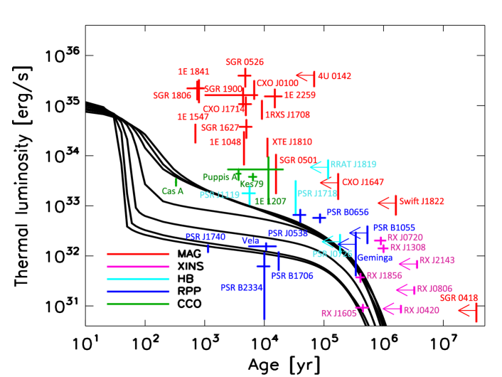
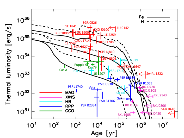
Figure 12: Comparison between observational data and theoretical cooling curves (from Viganò et al. 2013). The observational estimates of (errorbars) or constraints on (arrows) the age and thermal luminosity correspond to Viganò et al. (2013) and Table 3. The abbreviations in the legend mark different classes of neutron stars with measured thermal radiation (MAG – magnetar candidates, XINS – X-ray isolated neutron stars, HB – high-$B$ radio pulsars, RPP – rotation powered pulsars, CCO – central compact objects; see Paper I). Upper panel: non-magnetic neutron stars with iron envelopes, with $M=(1.10$, 1.25, 1.32, 1.40, 1.48, 1.60, 1.70, 1.76) $M_{\odot}$ (lines from top to bottom). Lower panel: a neutron star with $M=1.4\,M_{\odot}$ and $R=11.6$ km, and three different cases with initial magnetic field at the pole $B=0$, $3\times 10^{14}$ G, and $3\times 10^{15}$ G. The magnetic field topology is that of Model A in Viganò et al. (2013) (crustal confined). We show results for iron envelopes (solid lines) and hydrogen envelopes (dashed lines).

In the upper panel of Fig. 12 we show cooling curves for non-magnetized neutron stars with masses ranging between 1.10 and 1.76 $M_{\odot}$ (lines from top to bottom). After $\approx 100$ yr, low mass stars ($M\lesssim 1.4M_{\odot}$) are brighter than high mass stars. For the high-mass family, $M\gtrsim 1.4M_{\odot}$, the Durca processes in the central part of the star result in fast cooling before one hundred years. Within the low-mass family, cooling curves are similar at early ages ($<100$ yr). The differences at $t\sim 10^{2}-10^{3}$ yr are due to the delayed transition of neutrons in the core to a superfluid state, which activates the PBF neutrino emission. After the effect of the transition to a superfluid core is finished, at $t\gtrsim 10^{3}$ yr, cooling curves for low-mass neutron stars tend to converge again, following the same curve independently of the mass.

We see that luminosities of some objects in the upper panel of Fig. 12 are systematically above the theoretical cooling curves. For the CCOs this discrepancy can be eliminated by considering accreted (more heat-transparent) blanketing envelopes, as the lowest dashed line in the lower panel of Fig. 12 demonstrates. However, the high-$B$ objects still remain systematically hotter than what the theory can explain at $B=0$. This provides strong evidence in favor of the scenario in which magnetic field decay powers their larger luminosity. In the lower panel we compare the observational data to theoretical cooling curves for different values of the initial magnetic field up to $3\times 10^{15}$ G. The most relevant effect of the inclusion of the magnetic field is that it allows to explain objects with high luminosities. Magnetic fields $B\gtrsim 10^{14}$ G are strong enough to noticeably heat up the crust and power the observed X-ray radiation. Another important difference is that the cooling timescale for strongly magnetized objects is several times larger than for the weakly magnetized neutron stars.

7 Conclusions

We have considered the basic physical ingredients needed for theoretical modeling neutron-star thermal evolution and briefly reviewed some recent results on cooling of magnetized neutron stars. The physics behind such thermal evolution is extremely rich. Clearly, we could not consider it in depth in a single review paper. However, the information that we have given, together with the references to the formulae and online resources elsewhere, should be sufficient to build a neutron-star cooling model involving only the simplest assumptions. We considered the basic equations that govern the mechanical and thermal structure of a neutron star and its thermal evolution, the main contributions to the physical quantities that enter these equations – namely, EoS and heat capacity, thermal conductivity, neutrino emissivity, the effects of baryon superfluidity and proton superconductivity and of strong magnetic fields. In addition, we present a novel fit to the relation between the internal and external temperatures and heat fluxes in the blanketing envelope, which includes the effects of neutrino emission from the crust and the effects of non-radial heat transport.

In this paper we have restricted ourselves by the $npe\mu$ matter, without either hyperons or “exotic” models that involve hyperon condensates, quark phases, mixed phases, or phase transitions. We hope that an interested reader should be able to study these issues in depth following the literature references that we have provided. We have not considered also the equations of magnetic-field evolution, coupled to the thermal evolution, which is especially important in magnetars. These equations are given, for instance, in the paper by Mereghetti et al. (2015) in this volume, where origin, evolution, and observational manifestations of magnetars are reviewed in depth.

Appendices

Appendix A. Electron thermal conductivities

In this Appendix, we briefly overview the physics of electron heat conduction in the neutron-star envelopes, which is the most important heat conduction mechanism as regards the neutron-star thermal evolution, in the case of $B=0$. The magnetic field effects on the heat conduction are considered in Sect. 4.4.

A.1 Weakly degenerate electron gas

In the case of non-degenerate and non-relativistic electrons (Spitzer and Härm 1953; Braginskiĭ 1958; Spitzer 1962), the effective energy-averaged electron-ion collision frequency is

$$\nu_{e\mathrm{i}}=\frac{4}{3}\sqrt{\frac{2\pi}{m_{e}}}\,\frac{Z^{2}e^{4}}{T^{3/2}}\,n_{\mathrm{i}}\Lambda_{e\mathrm{i}},$$ (A.1)

where $\Lambda_{e\mathrm{i}}$ is the Coulomb logarithm. In the considered case $\Lambda_{e\mathrm{i}}$ is a slowly varying function of density and temperature. Its precise value depends on the approximations used to solve the Boltzmann equation, but its order of magnitude is given by the elementary theory, where the Coulomb collision integral is truncated at small and large impact parameters of the electrons. Then $\Lambda_{e\mathrm{i}}\sim\ln(r_{\mathrm{max}}/r_{\mathrm{min}})$, where $r_{\mathrm{max}}$ and $r_{\mathrm{min}}$ are the maximum and minimum electron impact parameters. The parameter $r_{\mathrm{max}}$ can be set equal to the Debye screening length, $r_{\mathrm{max}}^{-2}=4\pi(n_{e}+Z^{2}n_{\mathrm{i}})e^{2}/T$. The second parameter can be estimated as $r_{\mathrm{min}}=\max(\lambda_{e},\,r_{\mathrm{cl}})$, where $\lambda_{e}$ (defined in Sect. 2.3) limits $r_{\mathrm{min}}$ in the high-temperature regime (where the Born approximation holds), and $r_{\mathrm{cl}}=Ze^{2}/T$ is the classical closest-approach distance of a thermal electron, which limits $r_{\mathrm{min}}$ in the low-temperature, quasiclassical regime.

A similar effective frequency

$$\nu_{ee}=\frac{8}{3}\sqrt{\frac{\pi}{m_{e}}}\,\frac{e^{4}}{T^{3/2}}\,n_{e}\Lambda_{ee}$$ (A.2)

characterizes the efficiency of the $ee$ collisions. If $\Lambda_{ee}\sim\Lambda_{e\mathrm{i}}$, then $\nu_{e\mathrm{i}}/\nu_{ee}\sim Z$, therefore for large $Z$ the $e\mathrm{i}$ collisions are much more efficient than the $ee$ collisions.

A.2 Strongly degenerate electron gas

A.2.1 Electron-ion scattering

The thermal conductivity of strongly degenerate electrons in a fully ionized plasma is given by Eq. (12) with $a=\pi^{2}/3$. In order to determine the effective collision frequency that enters this equation, we use the Matthiessen rule $\nu=\nu_{e\mathrm{i}}+\nu_{ee}$.

The effective electron-ion collision frequency can be written in the form (Lee 1950; Yakovlev and Urpin 1980)

$$\nu_{e\mathrm{i}}=\frac{4Zm_{e}^{\ast}e^{4}\Lambda_{e\mathrm{i}}}{3\pi\hbar^{3}}=\frac{Z\Lambda_{e\mathrm{i}}\,\sqrt{1+x_{\mathrm{r}}^{2}}}{5.7\times 10^{-17}\mbox{~{}s}}.$$ (A.3)

Lee (1950) gave an estimate of the Coulomb logarithm $\Lambda_{e\mathrm{i}}=\ln(r_{\mathrm{max}}/r_{\mathrm{min}})$, with the minimum impact parameter $r_{\mathrm{min}}=\hbar/2p_{\mathrm{F}}$ and the maximum impact parameter $r_{\mathrm{max}}=a_{\mathrm{i}}$. Yakovlev and Urpin (1980) calculated the conductivities for relativistic degenerate electrons, neglecting electron screening, and obtained a more accurate estimate $r_{\mathrm{max}}\approx 0.4a_{\mathrm{i}}$ in the liquid regime. In the solid regime, where the electrons scatter on phonons (collective ion excitations), Yakovlev and Urpin (1980) obtained different approximations for the two distinct cases, $\Theta_{\mathrm{D}}<T<T_{\mathrm{m}}$ and $T<\Theta_{\mathrm{D}}$.

Potekhin et al. (1999) derived a unified treatment of the electron conductivities in the Coulomb liquid and solid and described both regimes by Eq. (A.3). Then qualitatively, by order of magnitude, $\Lambda_{e\mathrm{i}}\sim 1$ in the ion liquid, and $\Lambda_{e\mathrm{i}}\sim T/T_{\mathrm{m}}$ in the Coulomb solid with a melting temperature $T_{\mathrm{m}}$. The effects of multiphonon scattering, electron screening, and non-Born corrections, have been taken into account, and the Coulomb logarithms in both liquid and solid phases have been fitted by a single analytical formula. A Fortran code and a table of thermal conductivities, based on this formalism, are available online.

At the conditions typical for the envelopes of neutron stars, the electron-phonon scattering proceeds mainly via the Umklapp processes, where the wave vector corresponding to the change of electron momentum lies outside the first Brillouin zone. Raikh and Yakovlev (1982) noticed that if $T\lesssim T_{\mathrm{U}}=T_{\mathrm{p}}Z^{1/3}\alpha_{\mathrm{f}}\sqrt{1+x_{\mathrm{r}}^{2}}/3x_{\mathrm{r}}$, then the Umklapp processes occur less often (“freeze out”). Then the scattering rate decreases. Raikh and Yakovlev (1982) assumed an extremely strong (exponential) decrease. This implied that at $T<T_{\mathrm{U}}$ the conductivity would be in practice determined by impurities and structure defects of the lattice, rather than by the electron-phonon scattering (Gnedin et al. 2001). However, Chugunov (2012) showed that distortion of electron wave functions due to interaction with the Coulomb lattice destroys this picture and strongly slows down the increase of the conductivity. As a result, the conductivities in neutron star envelopes can be treated neglecting the “freezing-out” of the Umklapp processes.

A.2.2 Electron-electron scattering

Although the electron-ion scattering is usually most important for degenerate plasmas, the electron-electron scattering still can be non-negligible for relatively light elements ($Z\lesssim 10$) (Lampe 1968). The expression of $\nu_{ee}$ for the relativistic degenerate electrons at $T\ll T_{\mathrm{p}}$ was obtained by Flowers and Itoh (1976). Urpin and Yakovlev (1980) extended it to higher temperatures, where $T_{\mathrm{p}}\lesssim T\ll\epsilon_{\mathrm{F}}$.

Shternin and Yakovlev (2006) reconsidered the problem including the Landau damping of transverse plasmons, neglected by the previous authors. This effect is due to the difference of the components of the polarizability tensor, responsible for screening the charge-charge and current-current interactions: the transverse current-current interactions undergo “dynamical screening.” Shternin and Yakovlev (2006) showed that the Landau damping of transverse plasmons strongly increases $\nu_{ee}$ in the domain of $x_{\mathrm{r}}\gtrsim 1$ and $T\ll T_{\mathrm{p}}$ and presented a new fit to $\nu_{ee}$ (also implemented in the code referenced in footnote 4).

A.3 The case of intermediate degeneracy

In the case where the electron gas is partially degenerate, that is $T\sim\epsilon_{\mathrm{F}}$, the thermal and electrical conductivities determined by the electron-ion scattering are satisfactorily evaluated by the thermal averaging procedure [Eq. (33) in Sect. 4.4.2]. For conductivities determined by the electron-electron collisions, there is no such averaging procedure, but we can use an interpolation between the two limiting cases,

$$\nu_{ee}=\nu_{ee}^{\mathrm{deg}}\frac{1+625\,(T/\epsilon_{\mathrm{F}})^{2}}{1+25\,T/\epsilon_{\mathrm{F}}+271\,(T/\epsilon_{\mathrm{F}})^{5/2}}.$$ (A.4)

A satisfactory accuracy of this interpolation has been verified by Cassisi et al. (2007).

A.4 Impurities and mixtures

If the plasma in an envelope is not a pure substance of a single chemical element, then the effective collision frequency $\nu_{e\mathrm{i}}$ should be modified. The required modification can be different, depending on the state of the plasma and on the amount of impurities. For example, Flowers and Itoh (1976), Yakovlev and Urpin (1980), and Itoh and Kohyama (1993) considered electron scattering by charged impurities in a Coulomb crystal. If the fraction of impurities is small and they are randomly distributed, then electron-impurity scattering can be treated as scattering by charge fluctuations, controlled by the impurity parameter $Q=\langle(Z-\langle Z\rangle)^{2}\rangle,$ where $\langle Z\rangle\equiv\sum_{j}Y_{j}Z_{j}$, $Y_{j}=n_{j}/\sum_{j}n_{j}$ is the number fraction of ions of the $j$th kind, and $Z_{j}$ is their charge number. Then, using the Matthiessen rule, one can obtain $\nu_{e\mathrm{i}}$ as a sum of the terms corresponding to the electron-phonon scattering in a homogeneous lattice and to the electron scattering by charge fluctuations. The effective relaxation time for the latter term is given by Eq. (A.3) with $Z\Lambda_{e\mathrm{i}}$ replaced by $\sum_{j}Y_{j}(Z_{j}-\langle Z\rangle)^{2}\Lambda_{j}/\langle Z\rangle$, where the Coulomb logarithm $\Lambda_{j}$ depends generally on $j$. Neglecting the differences between the Coulomb logarithms, one can thus simply replace $Z$ by $Q/\langle Z\rangle$ in Eq. (A.3) to estimate the conductivity due to electron scattering by charged impurities.

An alternative approach is relevant when there is no dominant ion species which forms a crystal (e.g., in a liquid, a gas, or a glassy alloy). In this case, one can use Eq. (A.3) with $Z^{2}n_{\mathrm{i}}\Lambda_{e\mathrm{i}}$ replaced by $\sum_{j}Z_{j}^{2}n_{j}\Lambda_{j}$. An approximation to $\Lambda_{j}$ based on the plasma “additivity rule” has been suggested by Potekhin et al. (1999). Neglecting the differences between the Coulomb logarithms, one arrives at Eq. (A.3) with $Z$ replaced by $\sqrt{\langle Z^{2}\rangle}$. If tabulated conductivities $\kappa_{j}$ for pure substances are used, then the best agreement with calculations based on the “additivity rule” is usually given by the estimate

$$\kappa\approx\frac{\sum_{j}Y_{j}Z_{j}\kappa_{j}}{\sum_{j}Y_{j}Z_{j}}\equiv\frac{\langle\kappa Z\rangle}{\langle Z\rangle}.$$ (A.5)

Appendix B. Temperature relations for envelopes of neutron stars with magnetic fields

Here we present an analytical fit to the temperature distribution over a surface of a neutron star with a non-accreted envelope and a dipole magnetic field. We have chosen $\rho_{\mathrm{b}}=10^{10}$ g cm^-3 and used the BSk21 EoS (Pearson et al. 2012) in the parametrized form (Potekhin et al. 2013). The numerical data have been produced with the 2D code of Viganò et al. (2013) for 5 values of internal temperature $T_{\mathrm{b}}$ from $10^{7}$ K to $10^{9}$ K, 5 values of the magnetic field at the pole $B_{\mathrm{p}}$ from $10^{11}$ G to $10^{15}$ G, and 20 values of magnetic colatitude $\theta$ at the surface of the neutron star from 0 to $\pi/2$. The use of the 2D code corrects the temperature distribution near the magnetic equator, because the non-radial heat flow increases the equatorial $T_{\mathrm{s}}$ as compared to the 1D model that was employed previously (see Fig. 11 in Sect. 5.2). These data have been supplemented with more detailed calculations at the magnetic pole ($\theta=0$) using the 1D code of Potekhin et al. (2007) for 36 values of $T_{\mathrm{b}}$ from $10^{6.5}$ K to $10^{10}$ K and 9 values of $B_{\mathrm{p}}$ from $10^{11}$ G to $10^{15}$ G. An important difference from the old results is the inclusion of the neutrino emission from the crust, which is especially important for the magnetars (see Sect. 5). Because of the 2D treatment and the allowance for neutrino emission, the new fit supersedes the previous one (Potekhin et al. 2003), whenever $B>10^{12}$ G or $T_{\mathrm{b}}\gtrsim 10^{8}$ K. We stress that its use is restricted by non-accreted (i.e., composed of heavy chemical elements) envelopes in the range of $10^{6.5}\mbox{~{}K}\lesssim T_{\mathrm{b}}\lesssim 10^{10}$ K and $B_{\mathrm{p}}\lesssim 10^{15}$ G, which is covered by the underlying numerical data. For envelopes with $B\lesssim 10^{12}$ G (either non-accreted or accreted), the previous fit can be used, however the surface temperature $T_{\mathrm{s}}$ (but not the flux at the inner boundary, $F_{\mathrm{b}}$ – see item 4 below) should be limited for hot stars according to Eq. (B.4) below.

The fit consists of 3 stages: (1) an expression for the surface temperature at the magnetic pole, $T_{\mathrm{p}}$, as function of $T_{\mathrm{b}}$, $g$, and $B_{\mathrm{p}}$; (2) an expression for the ratio of the polar to the equatorial surface temperatures, $T_{\mathrm{p}}/T_{\mathrm{eq}}$; (3) an expression for the dependence of $T_{\mathrm{s}}$ on the magnetic colatitude $\theta$. Since the thermal conductivities for quantizing magnetic fields (Sect. 4.4.2) are known for the electron-ion but not electron-electron collision mechanism, we multiplied $T_{\mathrm{s}}$ by a correction factor, obtained numerically from a comparison of the results of thermal-structure calculations with and without the $ee$ collisions at $B=0$. At the end of this Appendix we suggest a recipe for relating the flux $F_{\mathrm{b}}$ at the bottom of the heat-blanketing envelope to temperature $T_{\mathrm{s}}$ and thereby to $T_{\mathrm{b}}$.

1. At the magnetic pole, the effective surface temperature, neglecting neutrino emission from the crust, is approximately given by the expression

$$T_{\mathrm{p}}^{(0)}=\left[g_{14}(T_{1}^{4}+(1+0.15\sqrt{B_{12}})\,T_{0}^{4})\right]^{1/4}\times 10^{6}\mbox{~{}K},$$ (B.1)

where

$$T_{0}=(15.7T_{9}^{3/2}+1.36T_{9})^{0.3796},\quad T_{1}=1.13\,B_{12}^{\,0.119}T_{9}^{a},\quad a=0.337/(1+0.02\sqrt{B_{12}}),$$ (B.2)

$T_{9}=T_{\mathrm{b}}/10^{9}$ K, and $B_{12}=B_{\mathrm{p}}/10^{12}$ G. The limiting temperature, at which $T_{\mathrm{p}}(T_{\mathrm{b}})$ levels off due to the neutrino emission from the crust is approximately given by

$$T_{\mathrm{p}}^{\mathrm{(max)}}=(5.2g_{14}^{0.65}+0.093\sqrt{g_{14}\,B_{12}})\times 10^{6}\mbox{~{}K}.$$ (B.3)

The corrected surface temperature at the pole, which takes this limit into account, is reproduced by the expression

$$T_{\mathrm{p}}=T_{\mathrm{p}}^{(0)}\left[1+(T_{\mathrm{p}}^{(0)}/T_{\mathrm{p}}^{\mathrm{(max)}})^{4}\right]^{-1/4}$$ (B.4)

2. The ratio of the polar to equatorial surface temperatures can be roughly evaluated as

$$\frac{T_{\mathrm{p}}}{T_{\mathrm{eq}}}=1+\frac{(1230\,T_{9})^{3.35}\,B_{12}\,\sqrt{1+2B_{12}^{\,2}}}{(B_{12}+450\,T_{9}+119\,B_{12}\,T_{9})^{4}}+\frac{0.0066\,B_{12}^{\,5/2}}{T_{9}^{1/2}+0.00258\,B_{12}^{\,5/2}}.$$ (B.5)

The numerically calculated $T_{\mathrm{p}}/T_{\mathrm{eq}}$ ratio has a complex dependence on $T_{\mathrm{b}}$ and $B$ at $B>10^{13}$ G. In order to keep our fitting formulae relatively simple, we do not reproduce these oscillations, but instead force the ratio (B.5) to converge to some average value at $B\gg 10^{13}$ G. The numerical data oscillate in a complicated manner around this average, with deviations reaching up to 35%. For smaller fields, $B\lesssim 3\times 10^{12}$ G, Eq. (B.5) reproduces the numerical data with typical errors of several percent (up to 10%). Note that these significant deviations affect only nearly tangential field case, viz. the equatorial region, which is substantially colder than the rest of the surface. Therefore its contribution to the observed flux is usually not very important.

3. Finally, the dependence of the surface temperature on the magnetic colatitude $\theta$ is approximately described by the expression

$$\frac{T_{\mathrm{s}}(\theta)-T_{\mathrm{eq}}}{T_{\mathrm{p}}-T_{\mathrm{eq}}}=\frac{(1+a_{1}+a_{2})\cos^{2}\theta}{1+a_{1}\cos\theta+a_{2}\cos^{2}\theta},\quad\mbox{where~{}~{}}a_{1}=\frac{a_{2}T_{9}^{1/2}}{3},\quad a_{2}=\frac{10\,B_{12}}{T_{9}^{1/2}+0.1\,B_{12}\,T_{9}^{-1/4}}.$$ (B.6)

4. Note that the outer boundary condition to the thermal evolution equations (4) involves the relation between the heat flux density $F_{\mathrm{b}}$ through the boundary at $\rho=\rho_{\mathrm{b}}$ and the temperature $T_{\mathrm{b}}$ at this boundary. In the absence of the neutrino emission from the crust, this boundary condition is directly provided by the $T_{\mathrm{b}}$ – $T_{\mathrm{s}}$ relation, because in this case (in the plane-parallel approximation) $F_{\mathrm{b}}=\sigma_{\mathrm{SB}}T_{\mathrm{s}}^{4}$. It is not so if a significant part of the energy is carried from the outer crust by neutrinos. In this case we suggest to evaluate the flux through the boundary by the relation $F_{\mathrm{b}}=\sigma_{\mathrm{SB}}T_{\ast}^{4}$, where $T_{\ast}$ is given by the above approximations for $T_{\mathrm{s}}$, but without the correction (B.4).

References

- Aguilera et al. (2008) D.N. Aguilera, J.A. Pons, J.A. Miralles, Astron. Astrophys. 486, 255 (2008)
- Aguilera et al. (2009) D.N. Aguilera, V. Cirigliano, J.A. Pons, S. Reddy, R. Sharma, Phys. Rev. Lett. 102, 091101 (2009)
- Akmal et al. (1998) A. Akmal, V.R. Pandharipande, D.G. Ravenhall, Phys. Rev. C 58, 1804 (1998)
- Ainsworth et al. (1989) T.L. Ainsworth, J. Wambach, D. Pines, Phys. Lett. B 222, 173 (1989)
- Alpar et al. (1984) M.A. Alpar, D. Pines, P.W. Anderson, J. Shaham, Astrophys. J. 276, 325 (1984)
- Amundsen and Østgaard (1985a) L. Amundsen, E. Østgaard, Nucl. Phys. A 437, 487 (1985a)
- Amundsen and Østgaard (1985b) L. Amundsen, E. Østgaard, Nucl. Phys. A 442, 163 (1985b)
- Bahcall and Wolf (1965a) J.N. Bahcall, R.A. Wolf, Astrophys. J. 142, 1254 (1965a)
- Bahcall and Wolf (1965b) J.N. Bahcall, R.A. Wolf, Phys. Rev. 140, B1452 (1965b)
- Baiko (2009) D.A. Baiko, Phys. Rev. E 80, 046405 (2009)
- Baiko and Yakovlev (1999) D.A. Baiko, D.G. Yakovlev, Astron. Astrophys. 342, 192 (1999)
- Baiko et al. (1998) D.A. Baiko, A.D. Kaminker, A.Y. Potekhin, D.G. Yakovlev, Phys. Rev. Lett. 81, 5556 (1998)
- Baiko et al. (2001a) D.A. Baiko, P. Haensel, D.G. Yakovlev, Astron. Astrophys. 374, 151 (2001a)
- Baiko et al. (2001b) D.A. Baiko, A.Y. Potekhin, D.G. Yakovlev, Phys. Rev. E 64, 057402 (2001b)
- Balberg and Barnea (1998) S. Balberg, N. Barnea, Phys. Rev. C 57, 409 (1998)
- Baldo and Schulze (2007) M. Baldo, H.-J. Schulze, Phys. Rev. C 75, 025802 (2007)
- Baldo et al. (1992) M. Baldo, J. Cugnon, A. Lejeune, U. Lombardo, Nucl. Phys. A 536, 349 (1992)
- Baldo et al. (1998) M. Baldo, Ø. Elgarøy, L. Engvik, M. Hjorth-Jensen, H.-J. Schulze, Phys. Rev. C 58, 1921 (1998)
- Bardeen et al. (1957) J. Bardeen, L.N. Cooper, J.R. Schrieffer, Phys. Rev. 108, 1175 (1957)
- Baym and Pethick (1991) G. Baym, C. Pethick, Landau Fermi-Liquid Theory: Concepts and Applications. John Wiley & Sons, New York (1991)
- Baym et al. (1971) G. Baym, C. Pethick, P. Sutherland, Astrophys. J. 170, 299 (1971)
- Baym et al. (1969) G. Baym, C. Pethick, D. Pines, Nature 224, 673 (1969)
- Bezchastnov et al. (1997) V.G. Bezchastnov, P. Haensel, A.D. Kaminker, D.G. Yakovlev, Astron. Astrophys. 328, 409 (1997)
- Bisnovatyi-Kogan and Romanova (1982) G.S. Bisnovatyi-Kogan, M.M. Romanova, Sov. Phys. JETP 56, 243 (1982)
- Blaschke et al. (1995) D. Blaschke, G. Röpke, H. Schulz, A.D. Sedrakian, D.N. Voskresensky, Mon. Not. R. Astron. Soc. 273, 596 (1995)
- Bohr et al. (1958) A. Bohr, B.R. Mottelson, D. Pines, Phys. Rev. 110, 936 (1958)
- Bowyer et al. (1964a) S. Bowyer, E.T. Byram, T.A. Chubb, H. Friedman, Nature 201, 1307 (1964a)
- Bowyer et al. (1964b) S. Bowyer, E.T. Byram, T.A. Chubb, H. Friedman, Science 146, 912 (1964b)
- Braginskiĭ (1958) S.I. Braginskiĭ, Sov. Phys. JETP 6, 358 (1958)
- Brown et al. (1998) E.F. Brown, L. Bildsten, R.E. Rutledge, Astrophys. J. 504, L95 (1998)
- Broderick et al. (2000) A. Broderick, M. Prakash, J.M. Lattimer, Astrophys. J. 537, 351 (2000)
- Brown and Cumming (2009) E.F. Brown, A. Cumming, Astrophys. J. 698, 1020 (2009)
- Brown et al. (1988) G.E. Brown, K. Kudobera, D. Page, P.M. Pizzochero, Phys. Rev. D 37, 2042 (1988)
- Burrows and Lattimer (1986) A. Burrows, J.M. Lattimer, Astrophys. J. 307, 178 (1986)
- Cameron (1967) A.G.W. Cameron, Nature 215, 464 (1967)
- Carr (1961) W.J. Carr, Phys. Rev. 122, 1437 (1961)
- Cassisi et al. (2007) S. Cassisi, A.Y. Potekhin, A. Pietrinferni, M. Catelan, M. Salaris, Astrophys. J. 661, 1094 (2007)
- Chamel (2005) N. Chamel, Nucl. Phys. A 747, 109 (2005)
- Chamel (2012) N. Chamel, Phys. Rev. C 85, 035801 (2012)
- Chamel et al. (2012) N. Chamel, R.L. Pavlov, L.M. Mihailov, et al., Phys. Rev. C 86, 055804 (2012)
- Chamel et al. (2013) N. Chamel, D. Page, S.K. Reddy, Phys. Rev. C 87, 035803 (2013)
- Chang et al. (2010) P. Chang, L. Bildsten, P. Arras, Astrophys. J. 723, 719 (2010)
- Chatterjee et al. (2015) D. Chatterjee, T. Elghozi, J. Novak, M. Oertel, Mon. Not. R. Astron. Soc. 447, 3785 (2015)
- Chen et al. (1993) J.M.C. Chen, J.W. Clark, R.D. Davé, V.V. Khodel, Nucl. Phys. A 555, 59 (1993)
- Chiu and Salpeter (1964) H.-Y. Chiu, E.E. Salpeter, Phys. Rev. Lett. 12, 413 (1964)
- Chugunov (2012) A.I. Chugunov, Astron. Lett. 38, 25 (2012)