The cosmic merger rate density of compact objects: impact of star formation, metallicity, initial mass function and binary evolution

Abstract

We evaluate the redshift distribution of binary black hole (BBH), black hole – neutron star binary (BHNS) and binary neutron star (BNS) mergers, exploring the main sources of uncertainty: star formation rate (SFR) density, metallicity evolution, common envelope, mass transfer via Roche lobe overflow, natal kicks, core-collapse supernova model and initial mass function. Among binary evolution processes, uncertainties on common envelope ejection have a major impact: the local merger rate density of BNSs varies from $\sim{}10^{3}$ to $\sim{}20$ Gpc^-3 yr^-1 if we change the common envelope efficiency parameter from $\alpha_{\rm CE}=7$ to 0.5, while the local merger rates of BBHs and BHNSs vary by a factor of $\sim{}2-3$. The BBH merger rate changes by one order of magnitude, when $1\sigma$ uncertainties on metallicity evolution are taken into account. In contrast, the BNS merger rate is almost insensitive to metallicity. Hence, BNSs are the ideal test bed to put constraints on uncertain binary evolution processes, such as common envelope and natal kicks. Only models assuming values of $\alpha_{\rm CE}\gtrsim{}2$ and moderately low natal kicks (depending on the ejected mass and the SN mechanism), result in a local BNS merger rate density within the 90% credible interval inferred from the second gravitational-wave transient catalogue.

1 Introduction

Gravitational-wave (GW) observations give us an insight into the merger rate density of binary compact objects in the local Universe (Abadie et al., 2010; Abbott et al., 2016b, c, a, 2019a, 2019b). Based on the results of the first (O1) and the second observing runs (O2), the LIGO-Virgo collaboration (LVC) has inferred a local merger rate density $\mathcal{R}_{\rm BBH}\sim{}24-140~{}\text{Gpc}^{-3}~{}\text{yr}^{-1}$ and $\mathcal{R}_{\rm BHNS}<610~{}\text{Gpc}^{-3}~{}\text{yr}^{-1}$ for binary black holes (BBHs) and black hole – neutron star binaries (BHNSs), respectively (Abbott et al., 2019a, b).

While this paper was in the review stage, the LVC published 39 events observed during the first half of the third observing run (O3a, Abbott et al. 2020a). This leads to a sample of 50 binary compact object mergers from O1, O2 and O3a, known as the second GW transient catalogue (GWTC-2). From these new data and assuming the power law + peak mass distribution model (which is shown to be preferred by the data), the BBH merger rate density inside the 90% credible interval is estimated to be $\mathcal{R}_{\rm{BBH}}=23.9^{+14.9}_{-8.6}$ Gpc^-3 yr^-1 ($\mathcal{R}_{\rm{BBH}}=58^{+54}_{-29}$ Gpc^-3 yr^-1) if we exclude (include) the event GW190814 (Abbott et al., 2020b). Abbott et al. (2020c) inferred a BNS local merger rate density $\mathcal{R}_{\rm BNS}=250-2810~{}\text{Gpc}^{-3}~{}\text{yr}^{-1}$ from the two published binary neutron star (BNS) mergers, GW170817 (Abbott et al., 2017a, b) and GW190425 (Abbott et al., 2020c). This number has recently been revised to account for the entire O3a data, leading to a new estimate $\mathcal{R}_{\rm{BNS}}=320^{+490}_{-240}$ Gpc^-3 yr^-1 (Abbott et al., 2020b).

Moreover, the target sensitivity of third-generation ground-based GW interferometers, namely the Einstein Telescope in Europe and Cosmic Explorer in the US, will allow us to observe BBH mergers up to $z\gtrsim{}10$ and BNS mergers up to $z\gtrsim{}2$ (Punturo et al., 2010; Reitze et al., 2019; Kalogera et al., 2019; Maggiore et al., 2020). This will make possible to fully reconstruct the evolution of the merger rate with redshift, opening new perspectives on the study of binary compact objects.

From a theoretical perspective, several studies attempt to predict the cosmic merger rate evolution, based on either cosmological simulations (Lamberts et al., 2016; Lamberts et al., 2018; O’Shaughnessy et al., 2017; Schneider et al., 2017; Mapelli et al., 2017; Mapelli & Giacobbo, 2018; Mapelli et al., 2018, 2019; Toffano et al., 2019; Artale et al., 2019, 2020; Graziani et al., 2020) or semi-analytical models (O’Shaughnessy et al., 2010; Dominik et al., 2013, 2015; Belczynski et al., 2016; Eldridge & Stanway, 2016; Giacobbo & Mapelli, 2018, 2020; Boco et al., 2019; Eldridge et al., 2019; Baibhav et al., 2019; Neijssel et al., 2019; Vitale et al., 2019; Tang et al., 2020).

Overall, our current understanding of the merger rate evolution is hampered by large uncertainties. On the one hand, our knowledge of the cosmic star formation rate (SFR) (e.g., Madau & Dickinson, 2014; Madau & Fragos, 2017), and the metallicity evolution of stars (e.g. Maiolino et al., 2008; Rafelski et al., 2012; Madau & Dickinson, 2014; Maiolino & Mannucci, 2018; De Cia et al., 2018; Chruslinska et al., 2019, 2020) are affected by a number of observational uncertainties. On the other hand, the very process of binary compact object formation is still matter of debate (see, e.g. Mandel & Farmer 2018 and Mapelli 2018 for two recent reviews).

Several formation channels have been proposed for binary compact objects: binary evolution via common envelope (e.g., Tutukov & Yungelson, 1973; Bethe & Brown, 1998; Portegies Zwart & Yungelson, 1998; Belczynski et al., 2002; Belczynski et al., 2008; Voss & Tauris, 2003; Podsiadlowski et al., 2004; Belczynski et al., 2016; Eldridge & Stanway, 2016; Stevenson et al., 2017; Giacobbo & Mapelli, 2018; Kruckow et al., 2018; Vigna-Gómez et al., 2018; Spera et al., 2019; Tanikawa et al., 2020) or via chemical mixing (e.g., Marchant et al., 2016; de Mink & Mandel, 2016; Mandel & de Mink, 2016), dynamical evolution in triples (e.g., Antonini & Rasio, 2016; Antonini et al., 2017; Arca-Sedda et al., 2018; Fragione & Loeb, 2019), in young star clusters (e.g., Banerjee et al., 2010; Ziosi et al., 2014; Mapelli, 2016; Banerjee, 2017, 2020; Kumamoto et al., 2019; Di Carlo et al., 2019; Di Carlo et al., 2020; Rastello et al., 2020), in globular clusters (e.g., Portegies Zwart & McMillan, 2000; Downing et al., 2010; Rodriguez et al., 2015, 2016; Rodriguez & Loeb, 2018a; Samsing et al., 2014; Askar et al., 2017; Samsing, 2018; Fragione & Kocsis, 2018; Zevin et al., 2019; Fragione & Silk, 2020; Antonini & Gieles, 2020) and in galactic nuclei (e.g., O’Leary et al., 2009; Miller & Lauburg, 2009; McKernan et al., 2012; McKernan et al., 2018; Antonini & Rasio, 2016; Bartos et al., 2017; Stone et al., 2017; Rasskazov & Kocsis, 2019; Arca Sedda et al., 2020; Arca Sedda, 2020; Yang et al., 2019; Tagawa et al., 2019). Each of these formation channels will likely leave an imprint on the evolution of the merger rate density with redshift (e.g. Dominik et al. 2013, 2015; Mapelli et al. 2017; Mapelli & Giacobbo 2018; Rodriguez & Loeb 2018b; Choksi et al. 2018; Choksi et al. 2019; Eldridge et al. 2019; Yang et al. 2019; Kumamoto et al. 2020; du Buisson et al. 2020; Mapelli et al. 2020a; Santoliquido et al. 2020). In particular, the merger rate of BBHs can be dramatically affected by dynamics, because of BH masses favouring dynamical exchanges (Hills & Fullerton, 1980).

Even if we restrict our attention to just one possible formation channel, we are faced with major uncertainties. For example, we do not have a satisfactory picture of the process of common envelope. Most population-synthesis models describe it through a free parameter, $\alpha_{\rm CE}$, which was originally meant to indicate the fraction of orbital energy that is transferred to the envelope (Webbink, 1984). According to its original definition, $\alpha_{\rm CE}$ should assume only values $\leq{}1$ and still theoretical models suggest that values of $\alpha_{\rm CE}>1$ better describe the formation of BNSs (e.g., Mapelli & Giacobbo, 2018; Fragos et al., 2019; Giacobbo & Mapelli, 2020).

Here, we focus on the formation of binary compact objects in isolation, through common envelope evolution, and we investigate all the main sources of uncertainty that affect the merger rate density evolution. In particular, we account for uncertainties on the cosmic SFR, metallicity evolution, common envelope (by varying the $\alpha_{\rm CE}$ parameter over more than one order of magnitude), natal kicks, core-collapse supernova (SN) models, mass transfer efficiency and on the slope of the initial mass function. We use cosmo$\mathcal{R}$ate (Santoliquido et al., 2020), a semi-analytic code that combines information on cosmic SFR and metallicity evolution with catalogues of binary compact objects obtained via binary population-synthesis. cosmo$\mathcal{R}$ate is computationally optimised to extensively probe the parameter space.

2 Methods

2.1 Population synthesis

We use catalogues of isolated compact binaries from our population-synthesis code mobse (Mapelli et al., 2017; Giacobbo et al., 2018; Giacobbo & Mapelli, 2018). mobse includes an up-to-date model for the mass loss rate of massive hot stars, scaling as $\dot{M}\propto Z^{\beta}$, where $Z$ is the metallicity and $\beta$ depends on the Eddington ratio, as defined in Giacobbo et al. (2018).

The prescriptions for core-collapse SNe adopted in mobse come from Fryer et al. (2012) and have been slightly modified to enforce a minimum neutron star (NS) mass of $\approx{}1.23$ M_⊙ (Giacobbo & Mapelli, 2020). Here, we consider both the rapid and the delayed SN model described by Fryer et al. (2012). The two models differ only by the time when the explosion is launched, which is $\lesssim$ 250 ms ($\gtrsim{}500$ ms) after the bounce in the rapid (delayed) model. According to these models, stars with final carbon-oxygen mass $m_{\rm CO}\gtrsim{}11$ M_⊙ collapse to a BH directly. In terms of compact remnant masses, the main difference between the rapid and the delayed model is that the former enforces a mass gap between 2 and 5 M_⊙, while the latter does not.

Following Timmes et al. (1996) and Zevin et al. (2020), we compute neutrino mass loss for both NSs and BHs as

$$m_{\nu}{}=\min\left[\frac{\left(\sqrt{1+0.3\,{}m_{\rm bar}}-1\right)}{0.15},\,{}0.5\,{}{\rm M}_{\odot}\right],$$ (1)

where $m_{\rm bar}$ is the baryonic mass of the compact object. The resulting gravitational mass of the compact object is $m_{\rm rem}=m_{\rm bar}-m_{\nu}{}$. Prescriptions for pair instability SNe and pulsational pair instability SNe are also implemented, as described in Mapelli et al. (2020b). Our treatment for electron-capture SNe is described in Giacobbo & Mapelli (2019).

We consider different SN kick prescriptions, in order to assess their impact on the cosmic merger rate density. As our fiducial model, we adopt the natal kick prescription proposed by Giacobbo & Mapelli (2020):

$$v_{\text{kick}}=f_{\text{H05}}\frac{m_{\text{ej}}}{\langle m_{\text{ej}}\rangle}\frac{\langle m_{\text{NS}}\rangle}{m_{\text{rem}}},$$ (2)

where $f_{\text{H05}}$ is a random value extracted from a Maxwellian distribution with one-dimensional root mean square $\sigma_{\rm 1D}=265~{}$\mathrm{k}\mathrm{m}\mathrm{s}^{-1}$$ (Hobbs et al., 2005), $m_{\rm ej}$ is the mass of the ejecta, $m_{\rm rem}$ is the mass of the compact remnant, $\langle m_{\text{NS}}\rangle$ is the average NS mass and $\langle m_{\text{ej}}\rangle$ is the average mass of the ejecta associated with the formation of a NS of mass $\langle m_{\text{NS}}\rangle$ from single stellar evolution. Equation 2 provides the natal kick for both NSs and BHs, and for both electron-capture and core-collapse SNe. Since BHs that form from direct collapse have $m_{\rm ej}=0$, they receive no kick. This kick prescription matches the proper motions of young Galactic pulsars (Hobbs et al., 2005; Bray & Eldridge, 2016, 2018) and at the same time the merger rate density inferred from LVC (Tang et al., 2020; Giacobbo & Mapelli, 2020).

We also consider a simplified model in which the natal kick velocity is randomly drawn from a Maxwellian distribution with fixed one-dimensional root mean square $\sigma_{\rm 1D}$. We consider three different values of $\sigma_{\rm 1D}=265$, 150 and 50 km s^-1. In this simple model, the natal kicks of BHs and NSs are drawn from the same Maxwellian distribution, without accounting for direct collapse or fallback. Furthermore, we consider two alternative kick models. The model F12 (from Fryer et al. 2012) draws the natal kicks from a Maxwellian distribution with $\sigma_{\rm{1D}}=265$ km s^-1 and then modulates the kick magnitude as

$$v_{\rm kick}=(1-f_{\rm fb})\,{}f_{\rm H05},$$ (3)

where $f_{\rm{fb}}$ is the fraction of fallback defined as in Fryer et al. (2012). Finally, the model VG18 (from Vigna-Gómez et al. 2018) draws the kicks from two different Maxwellian distributions with $\sigma_{\rm{1D}}=265$ and 30 km s^-1 for NSs born via core-collapse and electron-capture SNe, respectively. Also in this model, the kick is then modulated by the amount of fallback using equation 3.

In the default version of mobse, mass transfer via Roche lobe overflow is described as in Hurley et al. (2002). This yields a nearly conservative mass transfer if the accretor is a non-degenerate star. Here, we introduce also an alternative model in which the mass accretion rate ($\dot{m}_{a}$) is described as

$$\dot{m}_{a}=\left\{\begin{array}[]{ll}f_{\rm MT}\,{}|\dot{m}_{d}|&\textrm{if the accretor is non-degenerate}\\ \\ \min{(f_{\rm MT}\,{}|\dot{m}_{d}|,\dot{m}_{\rm Edd})}&\text{otherwise},\end{array}\right.$$ (4)

where $\dot{m}_{d}$ is the mass loss rate by the donor star, $\dot{m}_{\rm Edd}$ is the Eddington accretion rate and $f_{\rm MT}\in{}[0,\,{}1]$ is the accretion efficiency. Here, we explore $f_{\rm MT}=0.1,\,{}0.5$ and 1.

Other binary evolution processes are implemented as described in Hurley et al. (2002) and Santoliquido et al. (2020). In this work, we assume that the common envelope (CE) ejection efficiency parameter, $\alpha_{\rm CE}$, can assume values from 0.5 and 10, while $\lambda_{\rm CE}$ is derived as described in Claeys et al. (2014).

In the fiducial model, the mass of the primary star in each binary system is randomly drawn from a Kroupa (2001) initial mass function (IMF), with minimum mass $5$ M_⊙ and maximum mass $150$ M_⊙. For stars with mass $>0.5$ M_⊙, the Kroupa IMF behaves as a power law $dN/dm\propto{}m^{-\alpha_{\rm IMF}}$ with $\alpha_{\rm IMF}=2.3$. We also explored different IMF slopes for stars with mass $>0.5$ M_⊙. In particular, we consider two cases in which $\alpha_{{\rm IMF}}=2.0$ and 2.7.

Table 1 provides a summary of the different runs performed in this work. We have considered 12 different stellar metallicities for each run: $Z=0.0002$, 0.0004, 0.0008, 0.0012, 0.0016, 0.002, 0.004, 0.006, 0.008, 0.012, 0.016, 0.02. For each run, we have simulated $10^{7}$ binaries per each metallicity comprised between $Z=0.0002$ and 0.002, and $2\times{}10^{7}$ binaries per each metallicity $Z\geq{}0.004$, since higher metallicities are associated with lower BBH and BHNS merger efficiency (e.g. Giacobbo & Mapelli 2018; Klencki et al. 2018). Thus, we have simulated $1.8\times{}10^{8}$ binaries per each run shown in Table 1.

In all runs, the orbital periods, eccentricities and mass ratios of binaries are drawn from Sana et al. (2012). In particular, we derive the mass ratio $q=m_{2}/m_{1}$ as $\mathcal{F}(q)\propto q^{-0.1}$ with $q\in[0.1-1]$, the orbital period $P$ from $\mathcal{F}(\Pi)\propto\Pi^{-0.55}$ with $\Pi=\log{(P/\text{day})}\in[0.15-5.5]$ and the eccentricity $e$ from $\mathcal{F}(e)\propto e^{-0.42}~{}~{}\text{with}~{}~{}0\leq e\leq 0.9$.

Table 1: Summary of the models.

Model Name	$\alpha_{\rm CE}$	Kick Model	SN Model	$f_{\rm MT}$	$\alpha_{\rm IMF}$
$\alpha 0.5$	0.5	Eq. 2	Delayed	H02	2.3
$\alpha 1$	1	Eq. 2	Delayed	H02	2.3
$\alpha 2$	2	Eq. 2	Delayed	H02	2.3
$\alpha 3$	3	Eq. 2	Delayed	H02	2.3
$\alpha 5$	5	Eq. 2	Delayed	H02	2.3
$\alpha 7$	7	Eq. 2	Delayed	H02	2.3
$\alpha 10$	10	Eq. 2	Delayed	H02	2.3
$\alpha 1$s265	1	$\sigma_{\rm 1D}=265$ km/s	Delayed	H02	2.3
$\alpha 5$s265	5	$\sigma_{\rm 1D}=265$ km/s	Delayed	H02	2.3
$\alpha 1$s150	1	$\sigma_{\rm 1D}=150$ km/s	Delayed	H02	2.3
$\alpha 5$s150	5	$\sigma_{\rm 1D}=150$ km/s	Delayed	H02	2.3
$\alpha 1$s50	1	$\sigma_{\rm 1D}=50$ km/s	Delayed	H02	2.3
$\alpha 5$s50	5	$\sigma_{\rm 1D}=50$ km/s	Delayed	H02	2.3
$\alpha$1F12	1	Eq. 3	Delayed	H02	2.3
$\alpha$5F12	5	Eq. 3	Delayed	H02	2.3
$\alpha$1VG18	1	$\sigma_{\rm{high}}=265$ km/s $\sigma_{\rm{low}}=30$ km/s	Delayed	H02	2.3
$\alpha$5VG18	5	$\sigma_{\rm{high}}=265$ km/s $\sigma_{\rm{low}}=30$ km/s	Delayed	H02	2.3
$\alpha 1$R	1	Eq. 2	Rapid	H02	2.3
$\alpha 5$R	5	Eq. 2	Rapid	H02	2.3
$\alpha 1$MT0.1	1	Eq. 2	Delayed	0.1	2.3
$\alpha 1$MT0.5	1	Eq. 2	Delayed	0.5	2.3
$\alpha 1$MT1.0	1	Eq. 2	Delayed	1.0	2.3
$\alpha 5$MT0.1	5	Eq. 2	Delayed	0.1	2.3
$\alpha 5$MT0.5	5	Eq. 2	Delayed	0.5	2.3
$\alpha 5$MT1.0	5	Eq. 2	Delayed	1.0	2.3
$\alpha 10$MT0.1	10	Eq. 2	Delayed	0.1	2.3
$\alpha 10$MT0.5	10	Eq. 2	Delayed	0.5	2.3
$\alpha 10$MT1.0	10	Eq. 2	Delayed	1.0	2.3
$\alpha 1$IMF2.0	1	Eq. 2	Delayed	H02	2.0
$\alpha 1$IMF2.7	1	Eq. 2	Delayed	H02	2.7
$\alpha 5$IMF2.0	5	Eq. 2	Delayed	H02	2.0
$\alpha 5$IMF2.7	5	Eq. 2	Delayed	H02	2.7

Column 1: model name. Column 2: parameter $\alpha_{\rm CE}$ of the CE. Column 3: kick model; runs $\alpha 1$s265/$\alpha 5$s265, $\alpha 1$s150/$\alpha 5$s150 and $\alpha 1$s50/$\alpha 5$s50 have natal kicks drawn from a Maxwellian distribution with root mean square $\sigma_{\rm 1D}=265$, 150 and 50 km s^-1, respectively; runs $\alpha$1F12 and $\alpha{}$5F12 adopt the natal kick model in eq. 3; runs $\alpha{}1$VG18 and $\alpha{}5$VG18 assume the same model as Vigna-Gómez et al. (2018); in all the other models, the kicks are calculated as in eq. 2. Column 4: core collapse SN model; models $\alpha 1$R and $\alpha 5$R adopt the rapid model from Fryer et al. (2012), while all the other models adopt the delayed model from the same authors. Column 5: accretion efficiency $f_{\rm MT}$ onto a non-degenerate accretor; H02 means that we follow the same formalism as in Hurley et al. (2002). For the other models, see eq. 4. Column 6: slope of the IMF; models $\alpha_{\rm IMF}$ of the IMF for $m>0.5$ M_⊙; $\alpha 1$K2.0, $\alpha 5$K2.0 ($\alpha 1$K2.7, $\alpha 5$K2.7) have $\alpha_{\rm IMF}=2.0$ ($\alpha_{\rm IMF}=2.7$). All the other models assume the "standard" slope $\alpha_{\rm IMF}=2.3$ (Kroupa, 2001).

2.2 Cosmic merger rate density

We model the cosmic merger rate density $\mathcal{R}(z)$ following Santoliquido et al. (2020):

$$\mathcal{R}(z)=\frac{{\rm d}~{}~{}~{}~{}~{}}{{\rm d}t_{\rm lb}(z)}\left[\int_{z_{\rm max}}^{z}\psi(z^{\prime})\,{}\frac{{\rm d}t_{\rm lb}(z^{\prime})}{{\rm d}z^{\prime}}\,{}{\rm d}z^{\prime}\int_{Z_{\rm min}}^{Z_{\rm max}}\eta(Z)\,{}\mathcal{F}(z^{\prime},z,Z)\,{}{\rm d}Z\right],$$ (5)

where $t_{\rm lb}(z)$ is the look-back time at redshift $z$, $Z_{\rm min}$ and $Z_{\rm max}$ are the minimum and maximum metallicity, $\psi{}(z^{\prime})$ is the cosmic SFR density at redshift $z^{\prime}$, $\mathcal{F}(z^{\prime},z,Z)$ is the fraction of compact binaries that form at redshift $z^{\prime}$ from stars with metallicity $Z$ and merge at redshift $z$, and $\eta(Z)$ is the merger efficiency, namely the ratio between the total number $\mathcal{N}_{\text{TOT}}(Z)$ of compact binaries (formed from a coeval population) that merge within an Hubble time ($t_{{\rm H}_{0}}\lesssim 14$ Gyr) and the total initial mass $M_{\ast}{}(Z)$ of the simulation with metallicity $Z$:

$$\eta(Z)=f_{\rm bin}f_{\rm IMF}\frac{\mathcal{N}_{\text{TOT}}(Z)}{M_{\ast}{}(Z)},$$ (6)

where $f_{\rm bin}=0.5$ is the binary fraction, and $f_{\rm IMF}$ is a correction factor that takes into account that only stars with mass $m>5$ M_⊙ are simulated. This parameter depends on the adopted IMF, in particular $f_{\rm IMF}=0.483$, 0.285 and 0.123 when $\alpha_{\rm IMF}=2.0$, 2.3 and 2.7 respectively. The cosmological parameters used in equation 5 are taken from Ade et al. (2016). The maximum considered redshift in equation 5 is $z_{\rm max}=15$.

The SFR density $\psi(z)$ is described as (Madau & Fragos, 2017):

$$\psi(z)=0.01\,{}\frac{(1+z)^{2.6}}{1+[(1+z)/3.2]^{6.2}}~{}\text{M}_{\odot}\,{}\text{Mpc}^{-3}\,{}\text{yr}^{-1}.$$ (7)

As detailed in Santoliquido et al. (2020), we assume that the errors follow a log-normal distribution with mean $\log{\psi{}(0)}=-2$ and standard deviation $\sigma_{\log{\psi}}=0.2$.

The normalisation of equation 7 is obtained for a Kroupa IMF with $\alpha_{\rm IMF}=2.3$. When we vary the slope of the IMF, we have to change the normalisation of eq. 7 (Madau & Dickinson, 2014). Thus, we re-scale the normalisation by multiplying equation 7 by a factor 0.58 and 2.40 for $\alpha_{\rm IMF}=2.0$ and 2.7, respectively (see, e.g., Klencki et al., 2018).

The average stellar metallicity $\mu{}(z)$ evolves with redshift as

$$\mu(z)=\log{\left(\frac{Z(z)}{Z_{\odot}}\right)}=\log{(a)}\,{}+\,{}b\,{}z,$$ (8)

where $a=1.04\pm{}\,{0.14}$ and $b=-0.24\pm{}0.14$, based on observational results (Gallazzi et al., 2008; De Cia et al., 2018). We refer to Santoliquido et al. (2020) for a discussion on the choice of $a$ and $b$.

We model the distribution of stellar metallicities $\log{(Z/{\rm Z}_{\odot})}$ at a given redshift as a normal distribution with mean value $\mu{}(z)$ from equation 8 and standard deviation $\sigma_{Z}=0.20$ dex as our fiducial value:

$$p(z^{\prime},Z)=\frac{1}{\sqrt{2\pi\,{}\sigma_{Z}^{2}}}\,{}\exp\left\{{-\,{}\frac{\left[\log{(Z/{\rm Z}_{\odot})}-\mu(z^{\prime})\right]^{2}}{2\,{}\sigma_{Z}^{2}}}\right\}.$$ (9)

In Section 3.7, we discuss the impact of a different choice of $\sigma_{Z}$ on the merger rate density. Previous works have calculated the metallicity evolution based on a number of different assumptions and have shown its importance for the estimate of the merger rate (e.g., Dominik et al. 2013, 2015; Belczynski et al. 2016; Lamberts et al. 2016; Mapelli et al. 2017; Mapelli & Giacobbo 2018; Neijssel et al. 2019; Baibhav et al. 2019; Chruslinska et al. 2019, 2020).

The fraction of compact binaries that form at redshift $z^{\prime}$ from stars with metallicity $Z$ and merge at redshift $z$ is thus given by

$$\mathcal{F}(z^{\prime},z,Z)=\frac{\mathcal{N}(z^{\prime},z,Z)}{\mathcal{N}_{\text{TOT}}(Z)}\,{}p(z^{\prime},Z),$$ (10)

where $\mathcal{N}(z^{\prime},z,Z)$ is the total number of compact binaries that merge at redshift $z$ and form from stars with metallicity $Z$ at redshift $z^{\prime}$.

We performed $2\times 10^{3}$ realisations of equation 5 per each model in Table 1. In each realisation, we randomly draw the normalisation value of the SFR density (equation 7), and the intercept and the slope of the average metallicity (equation 8) from three Gaussian distributions with mean (standard deviation) equal to $\log{\psi{}(0)}=-2$ ($\sigma_{\log{\psi}}=0.2$), $a=1.04$ ($\sigma_{a}=0.14$) and $b=-0.24$ ($\sigma_{b}=0.14$), respectively. For simplicity, the value of the intercept and that of the slope are drawn separately, assuming no correlation.

3 Results

3.1 Merger efficiency

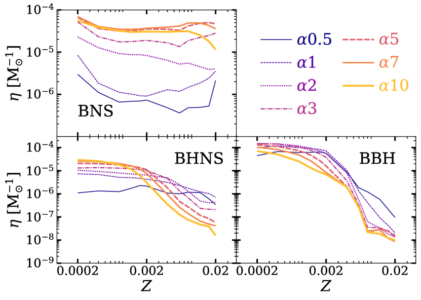
Figure 1: Merger efficiency $\eta$ as a function of progenitor’s metallicity for models $\alpha 0.5$ to $\alpha 10$. See Table 1 for further details.

Figure 1 shows the merger efficiency $\eta(Z)$ as defined in equation 6, as a function of progenitor’s metallicity and for different values of the $\alpha_{\rm CE}$ parameter. The BNS merger efficiency (hereafter, $\eta_{\rm BNS}$) mildly depends on the metallicity of the progenitor star, as already found by previous works (e.g., Mapelli et al., 2010; Chakrabarti et al., 2017; Giacobbo et al., 2018; Klencki et al., 2018; Chruslinska et al., 2018; Neijssel et al., 2019). The behaviour of $\eta{}_{\rm BNS}$ as a function of metallicity is different for different values of $\alpha_{\rm CE}$. For example, for $\alpha_{\rm CE}{}=1$, $\eta{}_{\rm BNS}$ has a U$-$shaped trend with metallicity and has a minimum at $Z=0.002$, while, for $\alpha_{\rm CE}{}=2$, $\eta{}_{\rm BNS}$ decreases almost monotonically from $Z=0.0002$ to $Z=0.02$. The BNS merger efficiency changes by less than one order of magnitude with $Z$, while it increases by two orders of magnitude with increasing $\alpha_{\rm CE}$. Thus, the BNS merger efficiency is strongly affected by the CE parameter $\alpha_{\rm CE}{}$ and only mildly affected by metallicity.

The behaviour of the BHNS merger efficiency (hereafter, $\eta_{\rm BHNS}$) as a function of metallicity dramatically depends on the value of $\alpha_{\rm CE}$. By decreasing the value of $\alpha_{\rm CE}$, $\eta{}_{\rm BHNS}$ progressively decreases at low $Z$ and increases at high $Z$. For large values of $\alpha_{\rm CE}$ ($\geq{}5$), $\eta_{\rm BHNS}$ decreases by three orders of magnitude going from $Z=0.0002$ up to $Z=0.02$, while for $\alpha_{\rm CE}=0.5$ $\eta_{\rm BHNS}$ is almost independent of $Z$.

This can be physically explained by an interplay between stellar winds and CE. A small value of $\alpha_{\rm CE}$ ($\alpha_{\rm CE}\lesssim 1$) means inefficient CE ejection: the binary has to shrink a lot before the envelope is ejected. At low $Z$, inefficient CE ejection suppresses the merger of small BHs (with mass $<10$ M_⊙), because their progenitor stars retain large envelopes and merge during CE, before giving birth to BHNSs. In contrast, at solar metallicity, stellar winds peel off stars and their envelopes are relatively small, making it difficult for CE to harden the system enough to merge by GW emission. Hence, an inefficient CE ejection tends to boost mergers of low-mass BHs at solar metallicity, by efficiently shrinking their progenitor binaries.

The BBH merger efficiency (hereafter, $\eta_{\rm BBH}$) strongly depends on progenitor’s metallicity and is only mildly affected by $\alpha_{\rm CE}$. $\eta_{\rm BBH}$ decreases by three–four orders of magnitude from the lowest to the highest considered metallicity. Lower values of $\alpha_{\rm CE}$ result in higher values of $\eta_{\rm BBH}$, with the exception of the case with $\alpha_{\rm CE}=0.5$ and $Z=0.0002$.

3.2 Common envelope

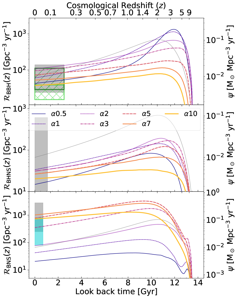
Figure 2: Left $y-$axis: Evolution of the merger rate density $\mathcal{R}(z)$ for BBHs (top), BHNSs (centre) and BNSs (bottom) in the comoving frame, as a function of the look-back time (lower $x-$axis) and of the redshift (upper $x-$axis). We vary $\alpha_{\rm CE}$ from 0.5 (model $\alpha 0.5$) to 10 (model $\alpha 10$). For both BBHs and BHNSs, the grey shaded area shows the 90% credible interval of the local merger rate density, as inferred from the first two observing runs of the LVC (Abbott et al., 2019a, b). For BBHs, we consider the union of the rates obtained with model A, B and C in Abbott et al. (2019b). For BNSs, the grey shaded area shows the merger rate density estimated in Abbott et al. (2020c). The hatched green areas in the upper panel show the local BBH merger rate density inferred including O3a events (Abbott et al., 2020b). In particular, the dark-green and light-green hatched areas show the 90% credible interval calculated including and excluding GW190814-like events, respectively (Abbott et al., 2020b). Finally, the cyan shaded area in the lower panel shows the 90% credible interval of the local BNS merger rate density, as estimated by Abbott et al. (2020b). The width of the shaded and hatched areas on the $x-$axis corresponds to the instrumental horizon obtained by assuming BBHs, BHNS, BNSs of mass $(10+10),(1.4-5)$ and $(1.4-1.4)$ M_⊙ respectively and O2 sensitivity (Abbott et al., 2018). Right $y-$axis and grey solid thin line: SFR density evolution (equation 7).

Figure 2 shows the cosmic merger rate density $\mathcal{R}(z)$ as a function of redshift for the same values of the CE parameter as shown in Figure 1. The BNS merger rate density is up to two orders of magnitude higher for large values of $\alpha_{\rm CE}$ than for low values. This trend can be easily explained by looking at the merger efficiency (Figure 1): for BNSs, larger values of $\alpha_{\rm CE}$ translate into higher merger efficiency.

The top panel of Figure 2 shows the merger rate density of BBHs. In the local Universe, $\mathcal{R}_{\rm BBH}(z)$ changes by a factor of $2-3$ if we change $\alpha_{\rm CE}$. Thus, the impact of $\alpha_{\rm CE}$ on the local BBH merger rate is smaller than in the case of BNSs. Moreover, models with large $\alpha_{\rm CE}$ result in lower BBH merger rates, with an opposite trend with respect to BNSs. These differences are also explained by the behaviour of the merger efficiency at different $\alpha_{\rm CE}$ (Figure 1).

The merger rate density of BHNSs follows an evolution similar to that of BBHs: lower values of $\alpha_{\rm CE}$ give higher merger rates (with the exception of $\alpha_{\rm CE}=0.5$) and the difference between models with different $\alpha_{\rm CE}$ is only a factor of $\sim{}2$ in the local Universe. As for BNSs and BBHs, this trend can be explained by looking at the merger efficiency. From now on, we consider $\alpha_{\rm CE}=1$ and 5 as our fiducial cases.

In Figure 2 and following, we show the 90% credible intervals inferred by the LVC. The grey boxes represent the values inferred from the first and second observing runs (GWTC-1, Abbott et al. 2019a) for BBHs ($\mathcal{R}_{\rm{BBH}}=24-140$ Gpc^-3 yr^-1), BHNSs ($\mathcal{R}_{\rm{BHNS}}\leq 610$ Gpc^-3 yr^-1) and BNSs ($\mathcal{R}_{\rm{BNS}}=250-2810$ Gpc^-3 yr^-1). From GWTC-2 (Abbott et al., 2020a), we considered the 90% credible intervals inferred for BBHs, with and without taking into account GW190814, which are $\mathcal{R}_{\rm{BBH}}=23.9^{+14.9}_{-8.6}$ Gpc^-3 yr^-1 (hatched light-green box) and $\mathcal{R}_{\rm{BBH}}=58^{+54}_{-29}$ Gpc^-3 yr^-1 (hatched dark-green box), respectively. The cyan box is the updated 90% credible interval inferred for BNSs, which is equal to $\mathcal{R}_{\rm{BNS}}=320^{+490}_{-240}$ Gpc^-3 yr^-1.

3.3 Natal kicks

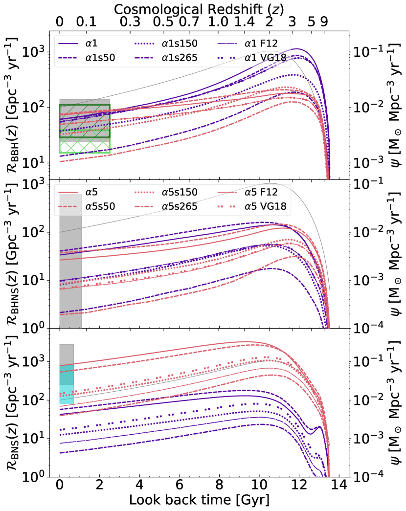
Figure 3: Merger rate density of BBHs (top), BHNSs (centre) and BNSs (bottom). Same as Figure 2, but we compare different natal kicks.

Figure 3 shows that the higher the natal kick is, the lower is the merger rate density at each given redshift, for BBHs, BHNSs and BNSs. In fact, high natal kicks tend to disrupt the binary system. SN kicks drawn from a Maxwellian distribution with $\sigma_{\rm 1D}=50~{}$kms^-1 yield a merger rate density similar to that given by equation 2.

As expected from the binary binding energy, the effect of different SN natal kick prescriptions is higher for BNSs, where there is a difference up to an order of magnitude if we consider natal kicks drawn from a Maxwellian with $\sigma_{\rm 1D}=265$km s^-1 with respect to $\sigma_{\rm 1D}=50$ km s^-1.

Only models with relative low natal kicks and large values of $\alpha_{\rm CE}$ (like $\alpha{}5$, $\alpha{}5$s50, $\alpha{}5$s150, and $\alpha{}5$VG18) are inside the 90% credible interval of GWTC-2 (Abbott et al., 2020a, b). On the other hand, a single Maxwellian curve with $\sigma_{\rm 1D}=50$ km s^-1 (e.g., models $\alpha{}1$s50 and $\alpha{}5$s50) is in tension with the observed proper motions of young pulsars in our Galaxy (Hobbs et al., 2005; Verbunt et al., 2017; Pol et al., 2019). Hence, only models $\alpha{}5$, $\alpha{}5$s150 and $\alpha{}5$VG18 are still consistent with both pulsars’ proper motions and GW data.

3.4 Core-collapse SN model

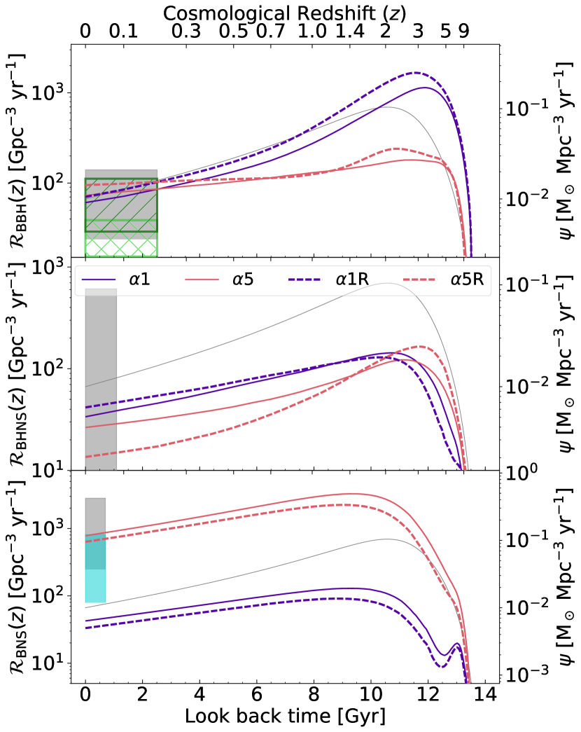
Figure 4: Merger rate density of BBHs (top), BHNSs (centre) and BNSs (bottom). Same as Figure 2, but we compare the rapid and delayed core-collapse SN models.

Choosing the delayed or the rapid core-collapse SN model has a minor impact on the cosmic merger rate density (Figure 4). The delayed model slightly enhances $\mathcal{R}_{\rm{BNS}}(z)$, because it produces more massive NSs which can merge on a shorter timescale. For the same reason, the delayed model slightly suppresses $\mathcal{R}_{\rm{BBH}}(z)$, because it produces a number of low-mass BHs ($3-5$ M_⊙), which merge on a longer timescale than more massive BHs. For BHNSs, the effect of the core-collapse SN model depends on the choice of the $\alpha_{\rm CE}$ parameter.

3.5 Mass accretion efficiency

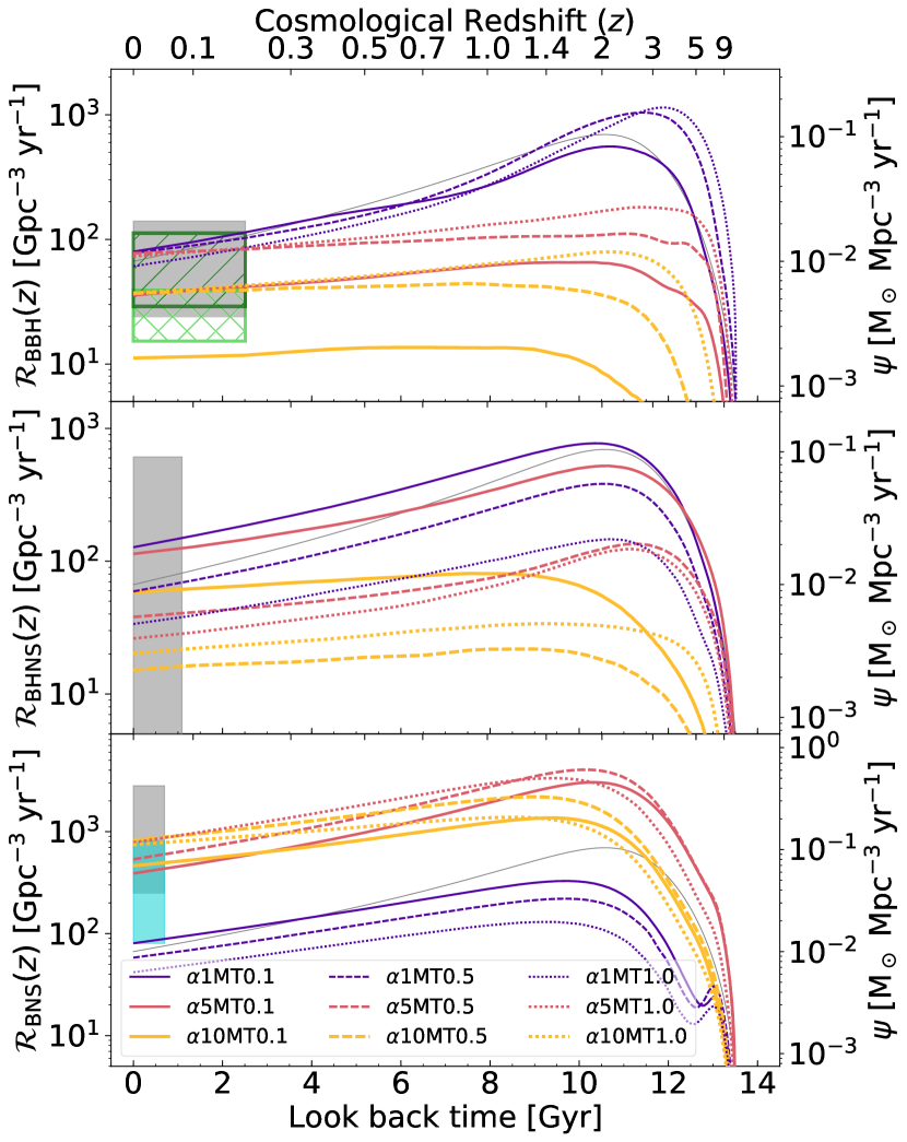
Figure 5: Merger rate density of BBHs (top), BHNSs (centre) and BNSs (bottom). Same as Figure 2, but we compare different values of the accretion efficiency parameter $f_{\rm MT}$.

Figure 5 shows the impact of different values of the mass accretion efficiency on the cosmic merger rate density. Lower values of $f_{\rm MT}$ result in a lower $\mathcal{R}_{\rm{BBH}}(z)$, especially for large values of $\alpha_{\rm CE}$. In contrast, lower values of $f_{\rm MT}$ lead to a higher $\mathcal{R}_{\rm{BHNS}}(z)$. Finally, the impact on BNS merger rate density is very mild and depends on $\alpha_{\rm CE}$.

The physical reason is that highly non-conservative mass accretion significantly reduces the total mass of the binary star. In particular, the secondary star accretes just a small fraction of the mass lost by the primary star during Roche lobe overflow. This implies that non-conservative mass transfer enhances the formation of unequal mass binary compact objects, such as BHNSs.

3.6 Initial mass function

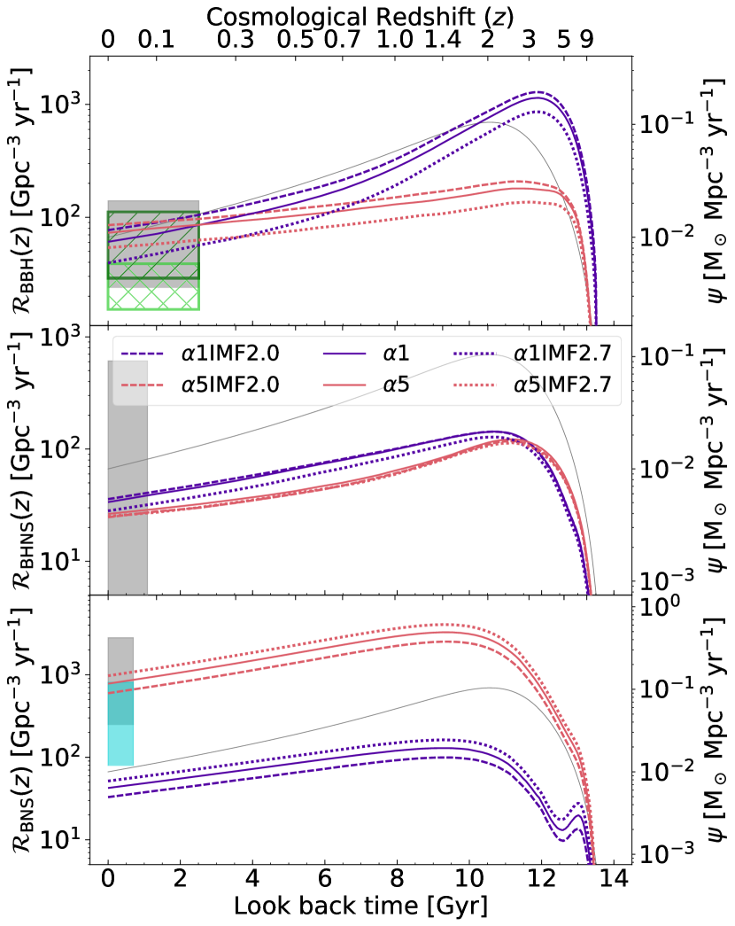
Figure 6: Merger rate density of BBHs (top), BHNSs (centre) and BNSs (bottom). Same as Figure 2, but we compare different values of the IMF slope $\alpha_{\rm IMF}$.

Figure 6 shows that the impact of varying the IMF’s slope on the cosmic merger rate is very mild, as already found by Klencki et al. (2018). $\mathcal{R}_{\rm{BBH}}(z)$ and $\mathcal{R}_{\rm{BNS}}(z)$ show an opposite trend: the former is higher when a shallower IMF slope is considered. This result has a trivial explanation: if $\alpha_{\rm IMF}=2.0$, the fraction of massive stars that end up collapsing into BHs is higher with respect to $\alpha_{\rm IMF}=2.7$.

3.7 Metallicity and SFR evolution

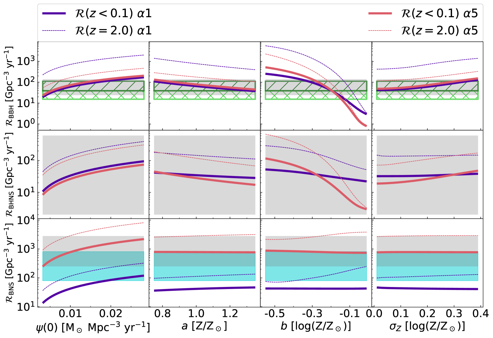
Figure 7: Merger rate density in the local Universe $\mathcal{R}(z<0.1)$ (thick line) and at $z=2$ (thin dashed line) as a function of the SFR density normalisation $\psi{}(0)$ (equation 7, leftmost column), the intercept $a$ and slope $b$ of the metallicity evolution model (equation 8, two central columns), and the metallicity spread $\sigma_{Z}$ (equation 9, rightmost column) for two different population-synthesis models: $\alpha 1$ and $\alpha 5$, as displayed in Table 1. For BBHs and BHNSs, the grey shaded area shows the 90% credible interval of the merger rate density in the local Universe, as inferred from the first two observing runs of the LVC. For BBHs, we consider the union of the rates obtained with model A, B and C in Abbott et al. (2019a, b). For BNSs, the grey shaded area shows the merger rate density estimated in Abbott et al. (2020c). The hatched green areas show the local BBH merger rate density inferred including O3a events (Abbott et al., 2020b). In particular, the dark-green and light-green hatched areas show the 90% credible interval calculated including and excluding GW190814-like events, respectively (Abbott et al., 2020b). Finally, the cyan shaded area shows the 90% credible interval of the local BNS merger rate density, as estimated by Abbott et al. (2020b).

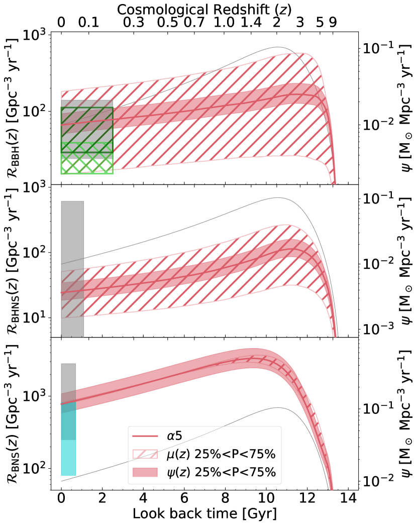
Figure 8: Merger rate density of BBHs (top), BHNSs (centre) and BNSs (bottom). Same as Figure 2, but we show the uncertainties on SFR and metallicity evolution. The contour areas represent 50% of different realisations (between the 25% and 75% percentile), while the thick solid line is the median. See Section 2.2 for details. To obtain the hatched area (with vertical lines), we varied only the slope and intercept of the metallicity fit (equation 8). To derive the shaded area we varied only the SFR density normalisation $\psi(0)$ (equation 7). Hence, the hatched area and the shaded area quantify the uncertainty on metallicity and SFR, respectively.

As we detailed in Section 2.2, the cosmic merger rate density is evaluated by assuming the fit from Madau & Fragos (2017) for the SFR density (equation 7) and a metallicity evolution model (equation 8). These two functions are affected by observational uncertainties; in this Section, we show their impact on the merger rate density. We take in account the uncertainty on four quantities, namely the normalisation factor of the SFR density $\psi(0)$ in equation 7, the intercept $a$ and slope $b$ of equation 8, and the metallicity spread $\sigma_{Z}$ in equation 9. We assume the metallicity spread $\sigma_{Z}$ to follow a log-normal distribution with standard deviation $0.1$ dex.

We evaluate the cosmic merger rate density by varying the value of the aforementioned parameters in a [$-2\sigma,+2\sigma$] interval, where $\sigma$ is the standard deviation associated with each parameter. We assume here, for simplicity, that the considered quantities follow a Gaussian distribution and that they are not correlated with each other.

Figure 7 shows the dependence of the merger rate density on these observational parameters. For sake of clarity, we just plotted the merger rate density in the local Universe ($z_{\rm loc}<0.1$) and at $z=2$ for two different values of $\alpha_{\rm CE}$. $\mathcal{R}_{\rm{BNS}}(z)$ is only mildly affected by the parameters that concern metallicity ($a$, $b$ and, $\sigma_{Z}$), especially at low redshift. The most important parameter for BNSs is the normalisation of the SFR $\psi{}(0)$. In order for the local merger rate density to be within the 90% credible interval inferred from the O1, O2 and O3a GW data collection, we have to assume a value of $\psi{}(0)\leq{}0.01~{}\rm{M}_{\odot}$ Mpc^-3 yr^-1 ($\psi{}(0)\geq{}0.02~{}\rm{M}_{\odot}$ Mpc^-3 yr^-1) for the model $\alpha{}5$ ($\alpha{}1$). Thus, the cosmic merger rate density of BNSs is mainly affected by population-synthesis uncertainties and by the uncertainty on the SFR.

In contrast, $\mathcal{R}_{\rm{BBH}}(z)$ changes by orders of magnitude when varying the parameters that describe metallicity evolution. For instance, if we assume $\sigma_{Z}>0.35$ ($0.29$) dex for model $\alpha 1$ ($\alpha 5$), while keeping the other parameters at their fiducial values, the local merger rate density of BBHs is outside the 90% credible interval inferred by the LVC from the GWTC-2, evaluated including GW190814-like events. We expect $\mathcal{R}_{\rm BBH}$ to grow with $\sigma_{Z}$ because a larger value of $\sigma_{Z}$ means that the percentage of metal-poor stars at low redshift is higher. As we have seen from Figure 1, the BBH merger efficiency is orders of magnitude higher for metal-poor stars. For the same reason, the cosmic merger rate density of BBHs decreases for increasing values of the intercept in equation 8.

The value of the slope $b$ in equation 8 represents the largest source of uncertainty for $\mathcal{R}_{\rm BBH}$, compared to the other observational parameters. The local BBH merger rate density changes by two to four orders of magnitude by varying $b$ within 2 $\sigma{}$. The local merger rate density is inside the 90% credible interval inferred from GWTC-2 only for $b\in{}[-0.19,-0.12]$ ($[-0.19,-0.15]$) for the model $\alpha 1$ ($\alpha 5$).

BHNSs behave in a similar way to BBHs, but all the considered realisations are still within the upper limit from the LVC.

Figure 8 shows the overall uncertainty affecting the cosmic merger rate density due to SFR and metallicity. We evaluate this uncertainty through the Monte Carlo method presented in Section 2.2. $\mathcal{R}_{\rm{BBH}}(z)$ and $\mathcal{R}_{\rm{BHNS}}(z)$ are heavily affected by uncertainties on metallicity evolution. In contrast, the uncertainty on $\mathcal{R}_{\rm{BNS}}(z)$ is much smaller and is dominated by the SFR.

3.8 Merger rate density as a function of metallicity

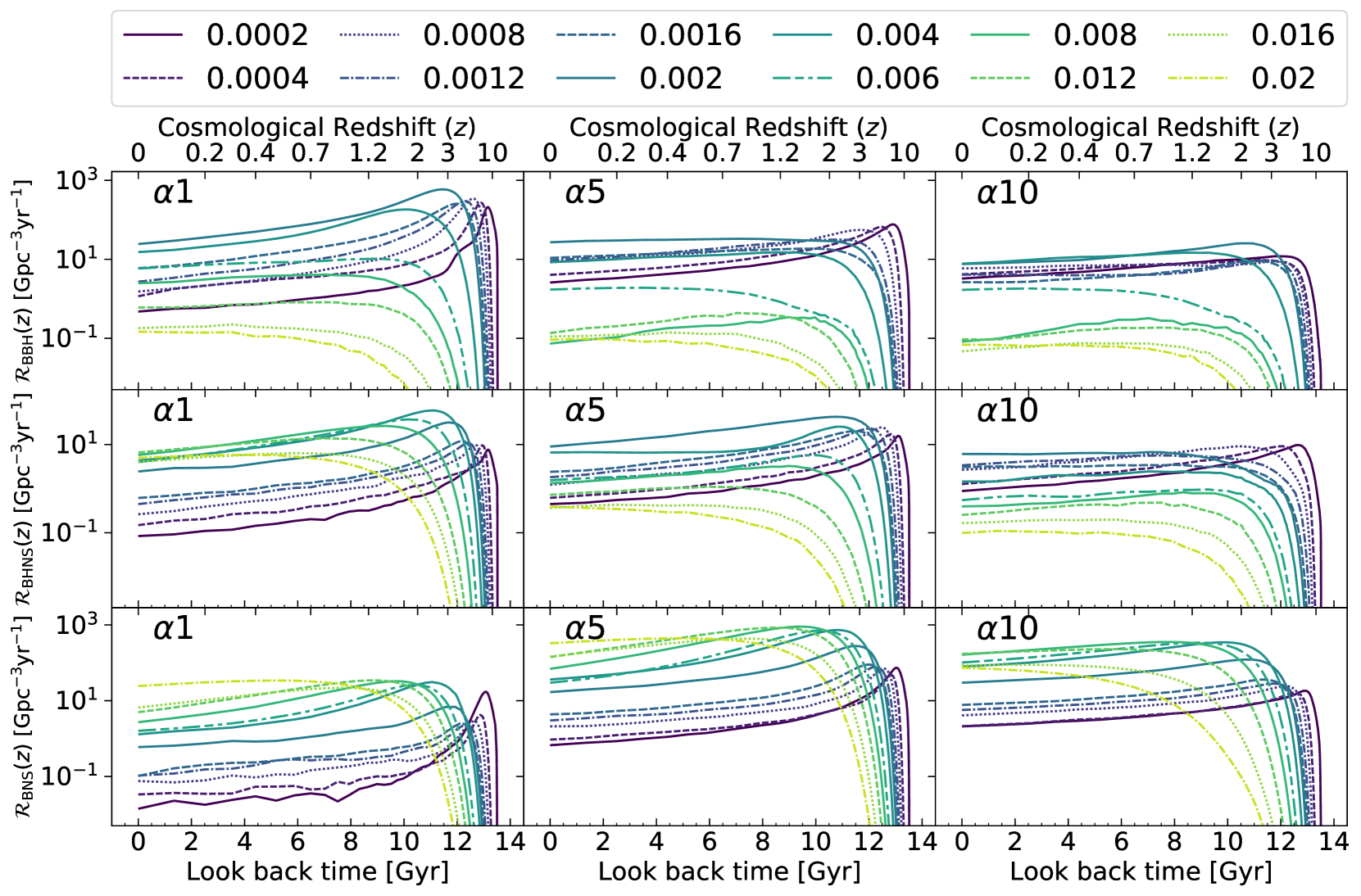
Figure 9: Contribution of progenitor’s metallicity to the cosmic merger rate density for three different population-synthesis model: $\alpha 1$, $\alpha 5$, and $\alpha 10$, as reported in Table 1. The considered metallicities are shown in the legend in the upper panel ($Z=0.0002-0.02$).

Figure 9 shows the contribution of different progenitor’s metallicities to the cosmic merger rate density, for three different values of $\alpha_{\rm CE}=1,$ 5 and 10. For $\alpha_{\rm CE}=1$, progenitor stars with $Z\sim{}0.004$ produce most of the BBHs merging at $z\lesssim{}4$.

In contrast, $\mathcal{R}_{\rm{BNS}}(z)$ is dominated by solar metallicity progenitors for $z\lesssim{}1$. Again, this springs from the different dependence of BBH and BNS merger efficiency on metallicity.

Different values of $\alpha_{\rm CE}$ change the relative contribution of different metallicities to the merger rate. For all kind of compact object binaries considered here (BBHs, BHNSs and BNSs), larger values of $\alpha_{\rm CE}$ correspond to a larger contribution of metal-poor stellar populations to the local merger rate with respect to metal-rich stellar populations. This happens because the delay times are generally longer for large values of $\alpha_{\rm CE}$ than for small values of $\alpha_{\rm CE}$. In fact, larger values of $\alpha_{\rm CE}$ imply that the CE is ejected without much shrinking of the binary system. Hence, the final binary that emerges from CE has a larger orbital separation, and needs more time to merge by GW emission.

4 Discussion

4.1 Fitting the merger rate density at z<1

Our models show that the merger rate density of binary compact objects is broadly reminiscent of the cosmic SFR density. Here, we want to quantify how close is the slope of the merger rate density to that of the cosmic SFR in our different models. Since LIGO and Virgo at design sensitivity will observe BBH mergers up to $z\sim{}1$, we restrict our attention to the slope of the merger rate density up to such redshift (Fishbach et al., 2018). We assume that $\mathcal{R}_{\rm BBH}(z)\propto{}(1+z)^{\lambda}{}$ if $z<1$. Under such assumption, we can fit the following quantities

$$\log{\left[\mathcal{R}(1+z)\right]}=\log{\mathcal{R}_{0}}+\lambda\,{}\log{(1+z)}.$$ (11)

We expect to find $\lambda{}\approx{}2.6$ if the merger rate density scales approximately with the cosmic SFR density, given equation 7.

Table 2: Coefficients of the fit in equation 11 with $0\leq{}z<1$ for each considered model.

Model name	BBH		BHNS		BNS
	$\mathcal{R}_{0}$	$\lambda$	$\mathcal{R}_{0}$	$\lambda$	$\mathcal{R}_{0}$	$\lambda$
$\alpha$0.5	40.39	1.56	14.74	2.12	21.75	1.04
$\alpha$1	57.74	2.16	34.45	1.57	44.59	1.50
$\alpha$2	105.42	1.33	29.58	1.60	76.54	1.95
$\alpha$3	94.08	1.19	30.10	1.47	358.44	1.97
$\alpha$5	73.76	0.83	25.74	1.28	812.20	1.92
$\alpha$7	52.08	0.74	26.88	1.00	1036.82	1.29
$\alpha$10	37.09	0.77	20.23	0.72	746.12	0.84
$\alpha$1s265	12.36	2.13	2.07	2.26	4.26	2.01
$\alpha$5s265	10.00	1.97	1.84	2.02	39.17	2.61
$\alpha$1s150	36.16	1.86	8.10	2.07	12.83	1.72
$\alpha$5s150	31.69	1.71	8.32	1.73	124.97	2.38
$\alpha$1s50	57.78	1.82	41.62	1.70	59.85	1.53
$\alpha$5s50	74.93	1.03	36.20	1.16	544.78	2.05
$\alpha$1F12	53.82	1.96	9.73	1.89	7.67	1.87
$\alpha$5F12	49.85	0.94	6.22	1.76	67.94	2.50
$\alpha$1VG18	54.07	1.95	9.61	1.89	17.31	1.93
$\alpha$5VG18	49.69	0.94	6.57	1.72	147.00	2.46
$\alpha$1R	65.28	2.52	42.54	1.31	35.31	1.41
$\alpha$5R	95.73	0.35	12.34	2.01	669.05	1.75
$\alpha$1MT0.1	83.03	1.71	128.04	2.05	82.99	1.77
$\alpha$5MT0.1	35.95	0.78	110.34	1.58	384.90	2.31
$\alpha$10MT0.1	11.39	0.31	59.69	0.48	464.31	1.42
$\alpha$1MT0.5	71.20	2.10	59.29	2.05	60.13	1.71
$\alpha$5MT0.5	77.70	0.43	37.36	0.96	535.59	2.36
$\alpha$10MT0.5	37.50	0.25	15.35	0.49	836.07	1.36
$\alpha$1MT1.0	58.47	2.13	34.06	1.58	43.88	1.53
$\alpha$5MT1.0	73.18	0.84	25.67	1.27	813.39	1.93
$\alpha$10MT1.0	36.99	0.78	20.55	0.69	761.75	0.90
$\alpha$1IMF2.0	72.98	2.07	36.70	1.49	34.60	1.48
$\alpha$5IMF2.0	84.34	0.83	24.07	1.29	620.73	1.92
$\alpha$1IMF2.7	37.45	2.25	28.28	1.62	53.97	1.55
$\alpha$5IMF2.7	53.71	0.86	24.36	1.26	1013.70	1.92

$\mathcal{R}_{0}$ is given in [Gpc^-3 yr^-1]. In order to check the goodness of the fits, we calculated the coefficient of determination $\rm R^{2}$ which is $>0.95$ for all the linear fits, except for the model $\alpha$5MT0.1, which yields $\rm R^{2}=0.84$.

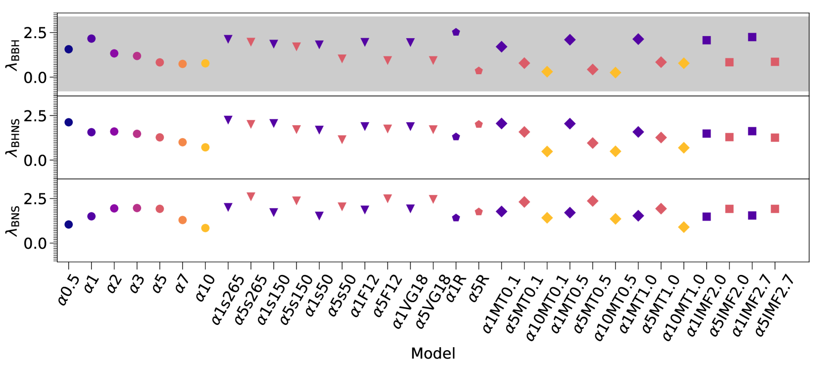
Figure 10: Values of $\lambda$ (defined in equation 11) for each considered model. From top to bottom: BBHs, BHNSs and BNSs. The grey shaded area represents the 90% credible interval of $\lambda{}_{\rm BBH}=1.3^{+2.1}_{-2.1}$, inferred by the LVC from GWTC-2, adopting the Power Law + Peak model (Abbott et al., 2020b).

We show the results of the fit for $z\in[0,1)$ in Table 2 and Figure 10. Most of our models have $\lambda{}<2.6$ for BBHs, BHNSs and BNSs. This suggests that the actual slope of the merger rate density is shallower than the one of the cosmic SFR, because of the delay time distribution, which encodes information on binary evolution processes, and because of the impact of metallicity on the merger efficiency.

The model closest to $\lambda=2.6$ is $\alpha 5$s265 for BNSs, i.e. the model with large natal kicks. With this kick choice, only the tightest and most massive systems can survive the SN explosion, and these systems are also those that merge with the shortest delay times by GW radiation. In contrast, the model with the shallowest slope is $\alpha 10$MT0.5 for BBHs, which yields $\lambda{}=0.25$. As we have already seen in Figure 9, models with $\alpha_{\rm CE}=10$ have longer delay times than the other models.

The slope $\lambda$ of each of considered model in this work is within the 90% credible interval inferred by the LVC (Abbott et al., 2020b) for BBHs, as also shown in Figure 10.

4.2 Merger efficiency and delay time impact on merger rate density

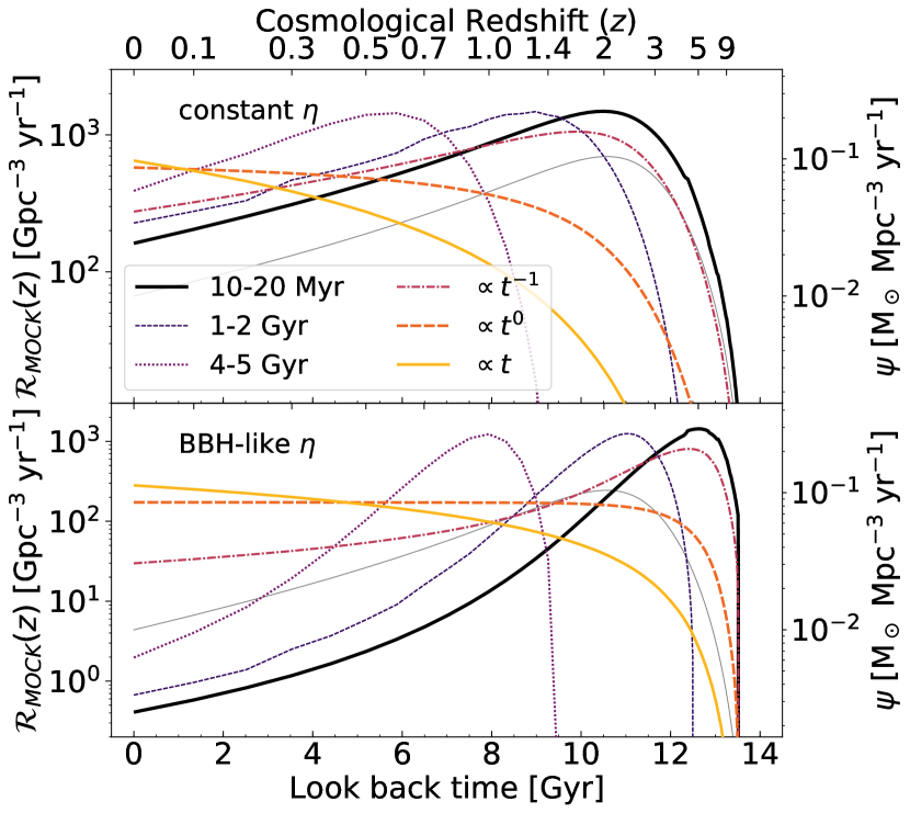
Figure 11: Evolution of the cosmic merger rate density evaluated with mock catalogues of merging compact binaries with constant (top) and BBH-like (bottom) merger efficiency $\eta$; and with six different delay time distributions. The thin grey line is the SFR from Madau & Fragos (2017).

In this Section, we want to use a simple toy model to interpret the results we found in the previous Section. In order to understand what are the effects on the cosmic merger rate density of the convolution of the SFR density with different delay time distributions and with metallicity, we performed some mock simulations.

The first ingredient of our mock simulations is the merger efficiency, which encodes a possible dependence on metallicity. We consider two different cases. In the first case, we assume a constant merger efficiency $\eta$, independent of metallicity; in the second case, we adopt a BBH-like $\eta$, higher at low metallicity. Specifically, for the latter case we use the merger efficiency of the $\alpha 5$ case, as displayed in Figure 1.

The second ingredient is the delay time $t_{\rm del}$ distribution. For simplicity, we assume that the delay time distribution does not depend on metallicity. We consider four cases in which we assume a uniform delay time distribution: three narrow distributions with $t_{\rm del}$ uniform from 10 to 20 Myr, from 1 to 2 Gyr and from 4 to 5 Gyr; and a broader distribution with $t_{\rm del}$ uniform from 10 Myr to 14 Gyr. Then, we consider two power law distributions: $\propto{}t^{-1}$ and $\propto{}t$, defined from 10 Myr to 14 Gyr.

Figure 11 shows the merger rate density evaluated with the aforementioned mock simulations. Let us start considering the cases with constant $\eta{}$. If the delay time is uniformly distributed between 10 and 20 Myr, the merger rate density has exactly the same slope and peak redshift as the cosmic SFR. The other two narrow delay time distributions have the effect to shift the merger rate density peak towards lower redshifts than the peak of the cosmic SFR. The case with $dN/dt\propto{}t^{-1}$ has a very similar slope to the cosmic SFR density ($\lambda\sim{}2.6$), while the cases with $dN/dt\propto{}t^{0}$ and $t$ have significantly flatter and even upturning slopes ($\lambda<0$). The case with constant $\eta$ and $\propto{}t^{-1}$ delay time distribution is reminiscent of our BNS simulations. However, the fact that our BNS models generally have a slope flatter than $\lambda{}=2.6$ (Table 2) tells us that, for a constant $\eta{}$, the delay time distribution in our models is flatter than $t^{-1}$.

Let us now look at the cases with a BBH-like $\eta{}$. The delay time distribution uniform between 10 and 20 Myr peaks at a higher redshift ($z_{\rm{peak}}\gtrsim{}5$) with respect to the cosmic SFR density. This happens because the BBH-like merger efficiency is maximum for metallicity $Z\sim{}0.0002$, which is common in the early Universe. This result is similar to our BBH models with $\alpha_{\rm CE}\leq{}1$ and is indicative of a strong dependence on metallicity combined with short delay times. For a uniform delay time distribution between 10 Myr and 14 Gyr, the merger rate density is almost constant with time, similar to the trend of $\mathcal{R}_{\rm BBH}(z)$ in the $\alpha 10$ model. Indeed, the delay time distribution of $\alpha 10$ is nearly flat, because $\alpha_{\rm CE}>5$ implies less effective shrinking of the binaries during CE, hence longer delay times.

4.3 Comparison with previous work

One of the main results of our analysis is that the BBH merger rate varies by more than one order of magnitude because of uncertainties on metallicity evolution, while the merger rate of BNSs is substantially unaffected by metallicity. This result is in agreement with previous studies (e.g. Giacobbo & Mapelli 2018; Chruslinska et al. 2019; Neijssel et al. 2019; Tang et al. 2020; Belczynski et al. 2020).

On top of that, the merger rates of BBHs, BHNSs and BNSs strongly depend on CE efficiency ($\alpha_{\rm CE}$), mass transfer efficiency ($f_{\rm MT}$) and natal kicks. For the merger rate of BBHs, the uncertainty connected with such binary evolution parameters is of the same order of magnitude as the uncertainty on metallicity evolution, consistent with Neijssel et al. (2019) and Belczynski et al. (2020). In these previous studies, the authors pointed out the importance of inter-parameter degeneracy while deriving astrophysical conclusions from GW observations.

For a suitable choice of these binary evolution parameters (namely $\alpha_{\rm CE}\geq{}2$ and moderately low natal kicks), we find reasonable agreement between our models and the LVC rates after O1, O2 and O3a (Abbott et al., 2019a, b, 2020c, 2020b). In particular, only models with moderately low kicks (depending on the ejected mass and the SN model), such as these described by Giacobbo & Mapelli (2020), Tang et al. (2020), Zevin et al. (2020) and Vigna-Gómez et al. (2018), can match the BNS merger rate in the local Universe.

When we compare our results with models adopting the cosmic SFR and metallicity evolution from cosmological simulations (e.g., Lamberts et al., 2016; Mapelli et al., 2017; Mapelli & Giacobbo, 2018; Artale et al., 2020), we find more conspicuous differences. For example, Figure 12 shows the comparison between the merger rates estimated with cosmo$\mathcal{R}$ate and those estimated by Mapelli & Giacobbo (2018) and Artale et al. (2020), using the illustris (Vogelsberger et al., 2014b, a; Nelson et al., 2015) and the eagle cosmological simulation (Schaye et al., 2015), respectively.

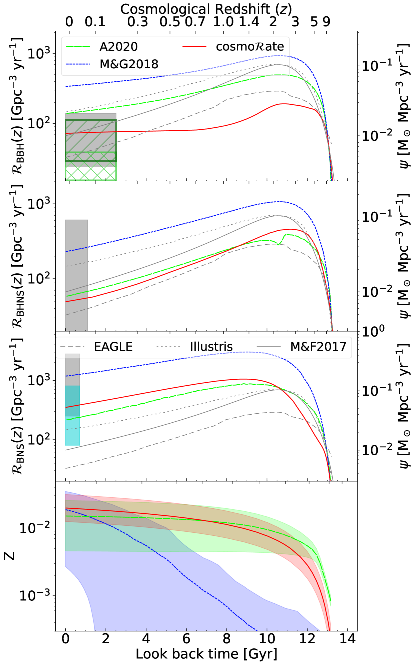
Figure 12: Comparison between the merger rate density of BBHs, BHNSs and BNSs obtained with cosmo$\mathcal{R}$ate (red solid lines) and the ones derived by Artale et al. (2020, green long-dashed lines with label A2020), based on the eagle cosmological simulation (Schaye et al., 2015), and by Mapelli & Giacobbo (2018, blue short dashed lines with label M&G2018), based on the illustris cosmological simulation (Vogelsberger et al., 2014b). Solid grey line: SFR density from Madau & Fragos (2017, with label M&F2017); long-dashed grey line: SFR density from the eagle simulation; short-dashed grey line: SFR density from the illustris simulation. The lower panel shows the average metallicity evolution in each model. Short-dashed blue line: illustris; long-dashed green line: eagle; solid red line: this work. The shaded area shows one standard deviation from the average metallicity.

To make a one-to-one comparison, we have re-run cosmo$\mathcal{R}$ate with the binary compact object catalogues from model CC15$\alpha 5$, obtained with an old version of mobse (see Giacobbo & Mapelli, 2018) and adopted in both Mapelli & Giacobbo (2018) and Artale et al. (2020). The merger rate density of BBHs, BHNSs and BNSs in the local Universe is a factor of $\sim{}3-5$ higher in Mapelli & Giacobbo (2018) than in this work. This difference is due to the cosmic SFR of the illustris cosmological simulation, which is a factor of $\sim{}2-2.5$ higher in the local Universe than the one described by Madau & Fragos (2017), and to the metallicity evolution of the illustris, which has a larger contribution from metal-poor stars (see the bottom panel of Figure 12). The results of cosmo$\mathcal{R}$ate are more similar to those reported in Artale et al. (2020). However, the cosmic SFR of the eagle is significantly lower than the one measured by Madau & Fragos (2017), as reported previously by Katsianis et al. (2017). This is compensated by the fact that the eagle average metallicity in the local Universe is lower with respect to equation 8.

5 Summary

We investigated the cosmic merger rate density evolution of compact binaries, by exploring the main sources of uncertainty. We have made use of the cosmo$\mathcal{R}$ate code (Santoliquido et al., 2020), which evaluates the cosmic merger rate density by combining catalogues of merging compact binaries, obtained from population-synthesis simulations, with the Madau & Fragos (2017) fit to the SFR density and with a metallicity evolution model based on De Cia et al. (2018) and Gallazzi et al. (2008).

We took into account uncertainties on the most relevant binary evolution processes: CE, SN kicks, core-collapse SN models and mass accretion by Roche lobe overflow. These represent the main bulk of uncertainty on the merger rate density due to binary evolution prescriptions. In addition, we varied the slope of the IMF. Our results confirm that the core-collapse SN model and the IMF produce negligible variations of the merger rate density.

The parameter $\alpha_{\rm CE}$, quantifying the efficiency of CE ejection, is one of the main sources of uncertainty. The merger rate density of BNSs spans up to 2 orders of magnitude if $\alpha_{\rm CE}$ varies from 0.5 to 10. For the same range of $\alpha_{\rm CE}$, $\mathcal{R}_{\rm{BHNS}}(z)$ and $\mathcal{R}_{\rm{BBH}}(z)$ vary up to a factor of 2 and 3, respectively. Only values of $\alpha_{\rm CE}\geq{}2$ give local BNS merger rate densities within the 90% credible interval inferred from GWTC-2 (Abbott et al., 2019a, b, 2020c) when we adopt our fiducial kick model.

Large natal kicks ($\sigma{}=265$ km s^-1) yield BNSs merger rate densities below the 90% credible interval from GWTC-2. Only models with moderately low kicks and large values of $\alpha_{\rm CE}$ (Bray & Eldridge, 2016, 2018; Vigna-Gómez et al., 2018; Giacobbo & Mapelli, 2020; Tang et al., 2020) predict values of the BNS merger rate within the 90% LVC credible interval inferred from GWTC-2.

Different values of the mass transfer efficiency parameter do not result in appreciable differences in the BNS merger rate density. The difference between $f_{\rm MT}=0.1$ and $f_{\rm MT}=1$ (conservative mass transfer) is up to a factor of $5-10$ for BHNSs and BBHs. The BBH local merger rate density with $f_{MT}=0.1$ can be as low as $\mathcal{R}_{\rm{BBH}}(z_{\rm{loc}}<0.1)\sim 11$ Gpc^-3 yr^-1 with $\alpha_{\rm CE}=10$, within the 90% credible interval inferred from GWTC-2 (Abbott et al., 2020a, b).

Callister et al. (2020) show that models with local merger rates $\mathcal{R}_{\rm BBH}(z)\propto{}(1+z)^{\lambda}{}$ with $\lambda{}\geq{}7$ are rejected, based on the O1 and O2 LVC data and on the analysis of the stochastic background. Recently, the LVC has reported $\lambda=1.3^{+2.1}_{-2.1}$ within the 90% credible interval, based on GWTC-2 (Abbott et al., 2020b). All of our models yield a slope $\lambda\leq{}2.6$ for $z<1$; hence, none of them can be rejected by current data. Most of our models are fitted by $\lambda{}\leq{}2$, a shallower slope with respect to the cosmic SFR. We show that this is indicative of a delay time distribution flatter than $t^{-1}$.

We have also investigated the effect of observational uncertainties on the cosmic SFR and on metallicity evolution. $\mathcal{R}_{\rm{BNS}}(z)$ is not significantly affected by metallicity evolution (Figure  8). In contrast, the metallicity evolution has a tremendous impact on the merger rate density of BBHs (Figure 8). $\mathcal{R}_{\rm{BBH}}(z)$ is inside the 90% credible interval inferred from GWTC-2 (considering GW190814-like events) only if the metallicity spread is $\sigma_{Z}\lesssim 0.35$.

By exploring 32 different models, we have varied only a small subset of all relevant model parameters, with sparse sampling of the many-dimensional space we considered. Hence, the effective uncertainty in the merger rate is likely higher than presented in our results. More exploration of the parameter space, and in particular of the $\alpha_{\rm CE}-$ natal kick space, is desirable in the future, even if it represents a computational challenge for population-synthesis models (e.g., Wong & Gerosa 2019).

In summary, the uncertainties on both cosmic metallicity and binary evolution processes substantially affect the merger rate of BBHs and BHNSs. As shown in previous work (e.g., Rodriguez & Loeb, 2018b; Santoliquido et al., 2020; Mapelli et al., 2020a), dynamics in dense star clusters represents another important source of uncertainty for the BBH merger rate.

In contrast, BNSs are not much affected by metallicity evolution and are not dramatically influenced by dynamics either, because they are significantly less massive than BBHs (Ye et al., 2020; Rastello et al., 2020; Santoliquido et al., 2020). Unlike BHs, for which the primordial BH formation channel has been proposed (Carr & Hawking, 1974; Carr et al., 2016), BNSs can originate only from the death of massive stars. This set of lucky circumstances gives us the opportunity to use the BNS merger rate to put constraints on some extremely uncertain binary evolution processes, such as mass transfer, common envelope and natal kicks.

Our results already point to an intriguing direction: only large values of $\alpha_{\rm CE}$ ($\geq{}2$) and moderately low natal kicks (depending on the ejected mass and the SN mechanism) can match the cosmic merger rate inferred from GWTC-2. The growing sample of GW events will help us deciphering this puzzle.

Data availability

The data underlying this article will be shared on reasonable request to the corresponding authors.

References

- Abadie et al. (2010) Abadie J., et al., 2010, Classical and Quantum Gravity, 27, 173001
- Abbott et al. (2016a) Abbott B. P., et al., 2016a, Physical Review X, 6, 041015
- Abbott et al. (2016b) Abbott B. P., et al., 2016b, Phys. Rev. Lett., 116, 061102
- Abbott et al. (2016c) Abbott B. P., et al., 2016c, ApJ, 818, L22
- Abbott et al. (2017a) Abbott B. P., et al., 2017a, Physical Review Letters, 119, 161101
- Abbott et al. (2017b) Abbott B. P., et al., 2017b, ApJ, 848, L12
- Abbott et al. (2018) Abbott B. P., et al., 2018, Living Reviews in Relativity, 21, 3
- Abbott et al. (2019a) Abbott B. P., et al., 2019a, Physical Review X, 9, 031040
- Abbott et al. (2019b) Abbott B. P., et al., 2019b, ApJ, 882, L24
- Abbott et al. (2020a) Abbott R., et al., 2020a, arXiv e-prints, p. arXiv:2010.14527
- Abbott et al. (2020b) Abbott R., et al., 2020b, arXiv e-prints, p. arXiv:2010.14533
- Abbott et al. (2020c) Abbott B. P., et al., 2020c, ApJ, 892, L3
- Ade et al. (2016) Ade P. A. R., Aghanim N., Zonca A. e. a., 2016, A&A, 594, A13
- Antonini & Gieles (2020) Antonini F., Gieles M., 2020, MNRAS, 492, 2936
- Antonini & Rasio (2016) Antonini F., Rasio F. A., 2016, ApJ, 831, 187
- Antonini et al. (2017) Antonini F., Toonen S., Hamers A. S., 2017, ApJ, 841, 77
- Arca Sedda (2020) Arca Sedda M., 2020, ApJ, 891, 47
- Arca-Sedda et al. (2018) Arca-Sedda M., Li G., Kocsis B., 2018, arXiv e-prints, p. arXiv:1805.06458
- Arca Sedda et al. (2020) Arca Sedda M., Mapelli M., Spera M., Benacquista M., Giacobbo N., 2020, ApJ, 894, 133
- Artale et al. (2019) Artale M. C., Mapelli M., Giacobbo N., Sabha N. B., Spera M., Santoliquido F., Bressan A., 2019, MNRAS, 487, 1675
- Artale et al. (2020) Artale M. C., Mapelli M., Bouffanais Y., Giacobbo N., Pasquato M., Spera M., 2020, MNRAS, 491, 3419
- Askar et al. (2017) Askar A., Szkudlarek M., Gondek-Rosińska D., Giersz M., Bulik T., 2017, MNRAS, 464, L36
- Baibhav et al. (2019) Baibhav V., Berti E., Gerosa D., Mapelli M., Giacobbo N., Bouffanais Y., Di Carlo U. N., 2019, Phys. Rev. D, 100, 064060
- Banerjee (2017) Banerjee S., 2017, MNRAS, 467, 524
- Banerjee (2020) Banerjee S., 2020, arXiv e-prints, p. arXiv:2004.07382
- Banerjee et al. (2010) Banerjee S., Baumgardt H., Kroupa P., 2010, MNRAS, 402, 371
- Bartos et al. (2017) Bartos I., Kocsis B., Haiman Z., Márka S., 2017, ApJ, 835, 165
- Belczynski et al. (2002) Belczynski K., Kalogera V., Bulik T., 2002, ApJ, 572, 407
- Belczynski et al. (2008) Belczynski K., Kalogera V., Rasio F. A., Taam R. E., Zezas A., Bulik T., Maccarone T. J., Ivanova N., 2008, ApJS, 174, 223
- Belczynski et al. (2016) Belczynski K., Holz D. E., Bulik T., O’Shaughnessy R., 2016, Nature, 534, 512
- Belczynski et al. (2020) Belczynski K., et al., 2020, A&A, 636, A104
- Berger et al. (2007) Berger E., et al., 2007, ApJ, 664, 1000
- Bethe & Brown (1998) Bethe H. A., Brown G. E., 1998, ApJ, 506, 780
- Boco et al. (2019) Boco L., Lapi A., Goswami S., Perrotta F., Baccigalupi C., Danese L., 2019, ApJ, 881, 157
- Bray & Eldridge (2016) Bray J. C., Eldridge J. J., 2016, MNRAS, 461, 3747
- Bray & Eldridge (2018) Bray J. C., Eldridge J. J., 2018, MNRAS, 480, 5657
- Callister et al. (2020) Callister T., Fishbach M., Holz D. E., Farr W. M., 2020, ApJ, 896, L32
- Carr & Hawking (1974) Carr B. J., Hawking S. W., 1974, MNRAS, 168, 399
- Carr et al. (2016) Carr B., Kühnel F., Sandstad M., 2016, Phys. Rev. D, 94, 083504
- Chakrabarti et al. (2017) Chakrabarti S., Chang P., O’Shaughnessy R., Brooks A. M., Shen S., Bellovary J., Gladysz W., Belczynski C., 2017, ApJ, 850, L4
- Choksi et al. (2018) Choksi N., Gnedin O. Y., Li H., 2018, MNRAS, 480, 2343
- Choksi et al. (2019) Choksi N., Volonteri M., Colpi M., Gnedin O. Y., Li H., 2019, ApJ, 873, 100
- Chruslinska et al. (2018) Chruslinska M., Belczynski K., Klencki J., Benacquista M., 2018, MNRAS, 474, 2937
- Chruslinska et al. (2019) Chruslinska M., Nelemans G., Belczynski K., 2019, MNRAS, 482, 5012
- Chruslinska et al. (2020) Chruslinska M., Jerabkova T., Nelemans G., Yan Z., 2020, arXiv e-prints, p. arXiv:2002.11122
- Claeys et al. (2014) Claeys J. S. W., Pols O. R., Izzard R. G., Vink J., Verbunt F. W. M., 2014, A&A, 563, A83
- De Cia et al. (2018) De Cia A., Ledoux C., Petitjean P., Savaglio S., 2018, A&A, 611, A76
- Di Carlo et al. (2019) Di Carlo U. N., Giacobbo N., Mapelli M., Pasquato M., Spera M., Wang L., Haardt F., 2019, MNRAS, 487, 2947
- Di Carlo et al. (2020) Di Carlo U. N., et al., 2020, arXiv e-prints, p. arXiv:2004.09525
- Dominik et al. (2013) Dominik M., Belczynski K., Fryer C., Holz D. E., Berti E., Bulik T., Mandel I., O’Shaughnessy R., 2013, ApJ, 779, 72
- Dominik et al. (2015) Dominik M., et al., 2015, ApJ, 806, 263
- Downing et al. (2010) Downing J. M. B., Benacquista M. J., Giersz M., Spurzem R., 2010, MNRAS, 407, 1946
- Eldridge & Stanway (2016) Eldridge J. J., Stanway E. R., 2016, MNRAS, 462, 3302
- Eldridge et al. (2019) Eldridge J. J., Stanway E. R., Tang P. N., 2019, MNRAS, 482, 870
- Fishbach et al. (2018) Fishbach M., Holz D. E., Farr W. M., 2018, ApJ, 863, L41
- Fragione & Kocsis (2018) Fragione G., Kocsis B., 2018, Phys. Rev. Lett., 121, 161103
- Fragione & Loeb (2019) Fragione G., Loeb A., 2019, MNRAS, 486, 4443
- Fragione & Silk (2020) Fragione G., Silk J., 2020, arXiv e-prints, p. arXiv:2006.01867
- Fragos et al. (2019) Fragos T., Andrews J. J., Ramirez-Ruiz E., Meynet G., Kalogera V., Taam R. E., Zezas A., 2019, ApJ, 883, L45
- Fryer et al. (2012) Fryer C. L., Belczynski K., Wiktorowicz G., Dominik M., Kalogera V., Holz D. E., 2012, ApJ, 749, 91
- Gallazzi et al. (2008) Gallazzi A., Brinchmann J., Charlot S., White S. D. M., 2008, MNRAS, 383, 1439
- Giacobbo & Mapelli (2018) Giacobbo N., Mapelli M., 2018, MNRAS, 480, 2011
- Giacobbo & Mapelli (2019) Giacobbo N., Mapelli M., 2019, MNRAS, 482, 2234
- Giacobbo & Mapelli (2020) Giacobbo N., Mapelli M., 2020, ApJ, 891, 141
- Giacobbo et al. (2018) Giacobbo N., Mapelli M., Spera M., 2018, MNRAS, 474, 2959
- Graziani et al. (2020) Graziani L., Schneider R., Marassi S., Del Pozzo W., Mapelli M., Giacobbo N., 2020, MNRAS, 495, L81
- Hills & Fullerton (1980) Hills J. G., Fullerton L. W., 1980, AJ, 85, 1281
- Hobbs et al. (2005) Hobbs G., Lorimer D. R., Lyne A. G., Kramer M., 2005, MNRAS, 360, 974
- Hurley et al. (2002) Hurley J. R., Tout C. A., Pols O. R., 2002, MNRAS, 329, 897
- Kalogera et al. (2019) Kalogera V., et al., 2019, BAAS, 51, 242
- Katsianis et al. (2017) Katsianis A., et al., 2017, MNRAS, 472, 919
- Klencki et al. (2018) Klencki J., Moe M., Gladysz W., Chruslinska M., Holz D. E., Belczynski K., 2018, A&A, 619, A77
- Kroupa (2001) Kroupa P., 2001, MNRAS, 322, 231
- Kruckow et al. (2018) Kruckow M. U., Tauris T. M., Langer N., Kramer M., Izzard R. G., 2018, preprint, (arXiv:1801.05433)
- Kumamoto et al. (2019) Kumamoto J., Fujii M. S., Tanikawa A., 2019, MNRAS, 486, 3942
- Kumamoto et al. (2020) Kumamoto J., Fujii M. S., Tanikawa A., 2020, arXiv e-prints, p. arXiv:2001.10690
- Lamberts et al. (2016) Lamberts A., Garrison-Kimmel S., Clausen D. R., Hopkins P. F., 2016, MNRAS, 463, L31
- Lamberts et al. (2018) Lamberts A., et al., 2018, MNRAS, 480, 2704
- Madau & Dickinson (2014) Madau P., Dickinson M., 2014, ARA&A, 52, 415
- Madau & Fragos (2017) Madau P., Fragos T., 2017, ApJ, 840, 39
- Maggiore et al. (2020) Maggiore M., et al., 2020, J. Cosmology Astropart. Phys., 2020, 050
- Maiolino & Mannucci (2018) Maiolino R., Mannucci F., 2018, arXiv e-prints,
- Maiolino et al. (2008) Maiolino R., et al., 2008, A&A, 488, 463
- Mandel & Farmer (2018) Mandel I., Farmer A., 2018, arXiv e-prints, p. arXiv:1806.05820
- Mandel & de Mink (2016) Mandel I., de Mink S. E., 2016, MNRAS, 458, 2634
- Mapelli (2016) Mapelli M., 2016, MNRAS, 459, 3432
- Mapelli (2018) Mapelli M., 2018, arXiv e-prints, p. arXiv:1809.09130
- Mapelli & Giacobbo (2018) Mapelli M., Giacobbo N., 2018, MNRAS, 479, 4391
- Mapelli et al. (2010) Mapelli M., Ripamonti E., Zampieri L., Colpi M., Bressan A., 2010, MNRAS, 408, 234
- Mapelli et al. (2017) Mapelli M., Giacobbo N., Ripamonti E., Spera M., 2017, MNRAS, 472, 2422
- Mapelli et al. (2018) Mapelli M., Giacobbo N., Toffano M., Ripamonti E., Bressan A., Spera M., Branchesi M., 2018, MNRAS, 481, 5324
- Mapelli et al. (2019) Mapelli M., Giacobbo N., Santoliquido F., Artale M. C., 2019, MNRAS, 487, 2
- Mapelli et al. (2020a) Mapelli M., Santoliquido F., Bouffanais Y., Arca Sedda M., Giacobbo N., Artale M. C., Ballone A., 2020a, arXiv e-prints, p. arXiv:2007.15022
- Mapelli et al. (2020b) Mapelli M., Spera M., Montanari E., Limongi M., Chieffi A., Giacobbo N., Bressan A., Bouffanais Y., 2020b, ApJ, 888, 76
- Marchant et al. (2016) Marchant P., Langer N., Podsiadlowski P., Tauris T. M., Moriya T. J., 2016, A&A, 588, A50
- McKernan et al. (2012) McKernan B., Ford K. E. S., Lyra W., Perets H. B., 2012, MNRAS, 425, 460
- McKernan et al. (2018) McKernan B., et al., 2018, ApJ, 866, 66
- Miller & Lauburg (2009) Miller M. C., Lauburg V. M., 2009, ApJ, 692, 917
- Nakar et al. (2006) Nakar E., Gal-Yam A., Fox D. B., 2006, ApJ, 650, 281
- Neijssel et al. (2019) Neijssel C. J., et al., 2019, MNRAS, 490, 3740
- Nelson et al. (2015) Nelson D., et al., 2015, Astronomy and Computing, 13, 12
- O’Leary et al. (2009) O’Leary R. M., Kocsis B., Loeb A., 2009, MNRAS, 395, 2127
- O’Shaughnessy et al. (2010) O’Shaughnessy R., Kalogera V., Belczynski K., 2010, ApJ, 716, 615
- O’Shaughnessy et al. (2017) O’Shaughnessy R., Bellovary J. M., Brooks A., Shen S., Governato F., Christensen C. R., 2017, MNRAS, 464, 2831
- Podsiadlowski et al. (2004) Podsiadlowski P., Langer N., Poelarends A. J. T., Rappaport S., Heger A., Pfahl E., 2004, ApJ, 612, 1044
- Pol et al. (2019) Pol N., McLaughlin M., Lorimer D. R., 2019, ApJ, 870, 71
- Portegies Zwart & McMillan (2000) Portegies Zwart S. F., McMillan S. L. W., 2000, ApJ, 528, L17
- Portegies Zwart & Yungelson (1998) Portegies Zwart S. F., Yungelson L. R., 1998, A&A, 332, 173
- Punturo et al. (2010) Punturo M., et al., 2010, Classical and Quantum Gravity, 27, 194002
- Rafelski et al. (2012) Rafelski M., Wolfe A. M., Prochaska J. X., Neeleman M., Mendez A. J., 2012, ApJ, 755, 89
- Rasskazov & Kocsis (2019) Rasskazov A., Kocsis B., 2019, ApJ, 881, 20
- Rastello et al. (2020) Rastello S., Mapelli M., Di Carlo U. N., Giacobbo N., Santoliquido F., Spera M., Ballone A., 2020, arXiv e-prints, p. arXiv:2003.02277
- Reitze et al. (2019) Reitze D., et al., 2019, in BAAS. p. 35 (arXiv:1907.04833)
- Rodriguez & Loeb (2018a) Rodriguez C. L., Loeb A., 2018a, ApJ, 866, L5
- Rodriguez & Loeb (2018b) Rodriguez C. L., Loeb A., 2018b, ApJ, 866, L5
- Rodriguez et al. (2015) Rodriguez C. L., Morscher M., Pattabiraman B., Chatterjee S., Haster C.-J., Rasio F. A., 2015, Physical Review Letters, 115, 051101
- Rodriguez et al. (2016) Rodriguez C. L., Chatterjee S., Rasio F. A., 2016, Phys. Rev. D, 93, 084029
- Samsing (2018) Samsing J., 2018, Phys. Rev. D, 97, 103014
- Samsing et al. (2014) Samsing J., MacLeod M., Ramirez-Ruiz E., 2014, ApJ, 784, 71
- Sana et al. (2012) Sana H., et al., 2012, Science, 337, 444
- Santoliquido et al. (2020) Santoliquido F., Mapelli M., Bouffanais Y., Giacobbo N., Di Carlo U. N., Rastello S., Artale M. C., Ballone A., 2020, arXiv e-prints, p. arXiv:2004.09533
- Schaye et al. (2015) Schaye J., et al., 2015, MNRAS, 446, 521
- Schneider et al. (2017) Schneider R., Graziani L., Marassi S., Spera M., Mapelli M., Alparone M., Bennassuti M. d., 2017, MNRAS, 471, L105
- Spera et al. (2019) Spera M., Mapelli M., Giacobbo N., Trani A. A., Bressan A., Costa G., 2019, MNRAS, 485, 889
- Stevenson et al. (2017) Stevenson S., Berry C. P. L., Mandel I., 2017, preprint, (arXiv:1703.06873)
- Stone et al. (2017) Stone N. C., Metzger B. D., Haiman Z., 2017, MNRAS, 464, 946
- Tagawa et al. (2019) Tagawa H., Haiman Z., Kocsis B., 2019, arXiv e-prints, p. arXiv:1912.08218
- Tang et al. (2020) Tang P. N., Eldridge J. J., Stanway E. R., Bray J. C., 2020, MNRAS, 493, L6
- Tanikawa et al. (2020) Tanikawa A., Susa H., Yoshida T., Trani A. A., Kinugawa T., 2020, arXiv e-prints, p. arXiv:2008.01890
- Timmes et al. (1996) Timmes F. X., Woosley S. E., Weaver T. A., 1996, ApJ, 457, 834
- Toffano et al. (2019) Toffano M., Mapelli M., Giacobbo N., Artale M. C., Ghirlanda G., 2019, MNRAS, 489, 4622
- Tutukov & Yungelson (1973) Tutukov A., Yungelson L., 1973, Nauchnye Informatsii, 27, 70
- Verbunt et al. (2017) Verbunt F., Igoshev A., Cator E., 2017, A&A, 608, A57
- Vigna-Gómez et al. (2018) Vigna-Gómez A., et al., 2018, MNRAS, 481, 4009
- Vitale et al. (2019) Vitale S., Farr W. M., Ng K. K. Y., Rodriguez C. L., 2019, ApJ, 886, L1
- Vogelsberger et al. (2014a) Vogelsberger M., et al., 2014a, MNRAS, 444, 1518
- Vogelsberger et al. (2014b) Vogelsberger M., et al., 2014b, Nature, 509, 177
- Voss & Tauris (2003) Voss R., Tauris T. M., 2003, MNRAS, 342, 1169
- Webbink (1984) Webbink R. F., 1984, ApJ, 277, 355
- Wong & Gerosa (2019) Wong K. W. K., Gerosa D., 2019, Phys. Rev. D, 100, 083015
- Yang et al. (2019) Yang Y., Bartos I., Haiman Z., Kocsis B., Márka Z., Stone N. C., Márka S., 2019, ApJ, 876, 122
- Ye et al. (2020) Ye C. S., Fong W.-f., Kremer K., Rodriguez C. L., Chatterjee S., Fragione G., Rasio F. A., 2020, ApJ, 888, L10
- Zevin et al. (2019) Zevin M., Samsing J., Rodriguez C., Haster C.-J., Ramirez-Ruiz E., 2019, ApJ, 871, 91
- Zevin et al. (2020) Zevin M., Spera M., Berry C. P. L., Kalogera V., 2020, arXiv e-prints, p. arXiv:2006.14573
- Zheng & Ramirez-Ruiz (2007) Zheng Z., Ramirez-Ruiz E., 2007, ApJ, 665, 1220
- Ziosi et al. (2014) Ziosi B. M., Mapelli M., Branchesi M., Tormen G., 2014, MNRAS, 441, 3703
- de Mink & Mandel (2016) de Mink S. E., Mandel I., 2016, MNRAS, 460, 3545
- du Buisson et al. (2020) du Buisson L., et al., 2020, arXiv e-prints, p. arXiv:2002.11630