The Einstein constraints: uniqueness and non-uniqueness in the conformal thin sandwich approach

Abstract

We study the appearance of multiple solutions to certain decompositions of Einstein’s constraint equations. Pfeiffer and York recently reported the existence of two branches of solutions for identical background data in the extended conformal thin-sandwich decomposition. We show that the Hamiltonian constraint alone, when expressed in a certain way, admits two branches of solutions with properties very similar to those found by Pfeiffer and York. We construct these two branches analytically for a constant-density star in spherical symmetry, but argue that this behavior is more general. In the case of the Hamiltonian constraint this non-uniqueness is well known to be related to the sign of one particular term, and we argue that the extended conformal thin-sandwich equations contain a similar term that causes the breakdown of uniqueness.

I Introduction

With the help of a 3+1 decomposition Einstein’s equations can be split into a set of constraint equations and a set of evolution equations Arnowitt et al. (1962); York, Jr. (1979). The four constraint equations – one in the Hamiltonian constraint and three in the momentum constraint – constrain the induced spatial metric $g_{ij}$ and the extrinsic curvature $K_{ij}$ on spatial hypersurfaces representing instants of constant coordinate time $t$. The constraint equations constrain only four of these initial variables; the remaining ones are freely specifiable and have to be chosen independently before the constraint equations can be solved. A decomposition of the initial data separates the freely specifiable variables from the constrained ones. Given a particular decomposition, the construction of initial data then entails making well-motivated choices for the freely specifiable independent background data and then solving the constraint equations for the constrained variables.

The conformal thin-sandwich decomposition has emerged as a particularly popular decomposition among numerical relativists, especially for the construction of quasi-equilibrium data (see, e.g., the reviews Cook (2000); Baumgarte and Shapiro (2003) and a brief discussion below). This variation of the original (non-conformal) thin-sandwich decomposition Belasco and Chanian (1969); Bartnik and Fodor (1993); Giulini (1999) was formally developed by York York, Jr. (1999) (see also Pfeiffer and York  Jr. (2003)), but more restricted versions had been introduced earlier Isenberg (1978); Wilson and Mathews (1989). It has been used, for example, for the construction of binary neutron stars (e.g. Baumgarte et al. (1997); Bonazzola et al. (1999); Uryū and Eriguchi (2000); Gourgoulhon et al. (2001)), binary black holes (e.g. Gourgoulhon et al. (2002); Grandclément et al. (2002); Yo et al. (2004); Cook and Pfeiffer (2004); Caudill et al. (2006)) and black hole-neutron star binaries (Baumgarte et al. (2004); K. Taniguchi, T. W. Baumgarte, J. A. Faber and S. L. Shapiro (2005)).

Given this wealth of experience with the conformal thin-sandwich decomposition, it came as quite a surprise when Pfeiffer and York (Pfeiffer and York  Jr. (2005), hereafter PY) recently discovered non-uniqueness in the solution of the conformal thin-sandwich system. Even for ‘small’ independent background data, which one would expect to generate gravitational initial data close to a flat slice of flat spacetime, the so-called “extended” set of conformal thin-sandwich data allowed for two branches of solutions. One of these two branches has comparatively weak gravitational fields and indeed approaches flat space in the limit of vanishing background data, while the second strong-field branch approaches a singular solution.

In this paper we discuss some of the aspects of this non-uniqueness. We consider a spherically symmetric, constant density star and show that even for this very simple model we can find – for sufficiently small values of the density – two branches of solutions. These two branches share some of the characteristics of the solutions found by PY and illustrate their properties. For our spherically symmetric solution the non-uniqueness of solutions is caused by a particular term having the “wrong sign” (see, e.g. York, Jr. (1979)), and we argue that the non-uniqueness found in the extended conformal thin-sandwich equations may be caused by a similar term.

We note also that certain constrained evolution schemes Choptuik et al. (2003); Rinne (2005) solve a set of elliptic equations at every timestep which is very similar to the extended conformal thin sandwich equations. These authors observed occasional failure of their elliptic solvers in the strong field regime, and it was argued Rinne (2005); Rinne and Stewart (2005) that this failure is caused by the “wrong sign” in the maximal slicing condition.

This paper is organized as follows. In Section II we briefly review the conformal thin-sandwich decomposition. We then consider the Hamiltonian constraint in spherical symmetry in Section III. First, in Sec. III.1, we construct analytic solutions for constant density stars and show that these solutions consist of two branches with properties very similar to the solutions found by PY. Subsequently, in Sec. III.2, we prove that at least some of these properties persist for arbitrary spherically symmetric solutions. Finally, we provide a brief summary and discussion in Section IV.

II The conformal thin-sandwich decompositions

Conformal decompositions of the constraint equations start with a conformal transformation of the spatial metric, $g_{ij}=\psi^{4}{\tilde{g}}_{ij}$, where $\psi$ is the conformal factor and ${\tilde{g}}_{ij}$ the conformally related metric. The Hamiltonian constraint then becomes an equation for the conformal factor

$${\tilde{\nabla}}^{2}\psi-\frac{1}{8}\tilde{R}\psi-\frac{1}{12}K^{2}\psi^{5}+\frac{1}{8}\psi^{-7}\tilde{A}^{ij}\tilde{A}_{ij}+2\pi\psi^{5}\rho=0.$$ (1)

Here ${\tilde{\nabla}}\!$ and $\tilde{R}$ are the covariant derivative and the trace of the Ricci tensor associated with ${\tilde{g}}_{ij}$, and the extrinsic curvature is decomposed into its trace $K$ and the conformally related trace-free part $\tilde{A}^{ij}$,

$$K^{ij}=\psi^{-10}\tilde{A}^{ij}+\frac{1}{3}g^{ij}K.$$ (2)

For completeness we have also included the matter source $\rho=n^{a}n^{b}T_{ab}$, where $n^{a}$ is the normal on the spatial hypersurface and $T_{ab}$ the stress-energy tensor, and where summation is carried out over four spacetime indices.

The matter term as written in Eq. (1) has the defect York, Jr. (1979) that its positive sign combined with the positive exponent of $\psi$ prevent use of the maximum principle to prove local uniqueness of solutions. Therefore, it is not immediately clear that solutions to Eq. (1) are unique (indeed, we show in Sec. III, that often they are not unique). This defect can be cured York, Jr. (1979) by introduction of a conformally scaled matter density $\tilde{\rho}=\psi^{8}\rho$; taking $\tilde{\rho}\geq 0$ as freely specifiable data, the matter term in Eq. (1) becomes $2\pi\psi^{-3}\tilde{\rho}$. Because of the sign-change in the exponent, this term is now well-behaved and the maximum principle is applicable. We will use Eq. (1) with the unscaled $\rho$ as a toy example in Sec. III below. Besides that, we are only interested in vacuum space-times and therefore do not include matter terms in the rest of this Section.

The conformal metric ${\tilde{g}}_{ij}$, meanwhile, is freely specifiable. In the conformal thin-sandwich decompositions, the time derivative of the conformal metric, $\tilde{u}_{ij}\equiv\partial_{t}{\tilde{g}}_{ij}$ is also considered freely specifiable. Using the evolution equation for the spatial metric we can relate $\tilde{u}_{ij}$ to $\tilde{A}_{ij}$,

$$\tilde{A}^{ij}=\frac{1}{2\tilde{N}}\Big{(}(\tilde{\mathbb{L}}{\beta})^{ij}-\tilde{u}^{ij}\Big{)},$$ (3)

where the conformal (or densitized) lapse $\tilde{N}$ is related to the lapse $N$ by $N=\psi^{6}\tilde{N}$. Inserting this expression into the momentum constraint yields

$${\tilde{\nabla}}\!_{j}\Big{(}\frac{1}{2\tilde{N}}(\tilde{\mathbb{L}}{\beta})^{ij}\Big{)}-\frac{2}{3}\psi^{6}{\tilde{\nabla}}^{i}K-{\tilde{\nabla}}\!_{j}\Big{(}\frac{1}{2\tilde{N}}\tilde{u}^{ij}\Big{)}=0$$ (4)

where $(\tilde{\mathbb{L}}{\beta})^{ij}\equiv 2{\tilde{\nabla}}^{(i}\beta^{j)}-2/3\,{\tilde{g}}^{ij}{\tilde{\nabla}}\!_{k}\beta^{k}$ is the conformal longitudinal operator.

There are two versions of the conformal thin sandwich approach. In the standard conformal thin sandwich equations, one specifies $({\tilde{g}}_{ij},\tilde{u}_{ij};K,\tilde{N})$ and suitable matter-terms, if applicable. Given these background variables, Eq. (1) and (4) (together with (3)) can be solved for the conformal factor $\psi$ and the shift $\beta^{i}$, which completes the set of initial data.

For maximal slices, $K=0$, Eqs. (1) and (4) decouple, so that Eq. (4) can be considered first. For any given strictly positive $\tilde{N}$, this equation is a linear elliptic equation so that the existence of a unique solution $\beta^{i}$ is guaranteed. This is a key motivation for the entire structure and is discussed in York, Jr. (1999); Pfeiffer and York  Jr. (2003). Eq. (1) – with zero matter density $\rho$ – becomes the standard Lichnerowicz equation for the conformal factor Lichnerowicz (1944) and again has a unique solution as long as the base metric is in the positive Yamabe class.

In the extended system one regards $\partial_{t}K$ instead of $\tilde{N}$ as freely specifiable. The lapse can then be solved for from the trace of the evolution equation for the extrinsic curvature, which often is written as

$${\tilde{\nabla}}^{2}(\tilde{N}\psi^{7})-(\tilde{N}\psi^{7}) \bigg{[}\frac{\tilde{R}}{8}\!+\!\frac{5}{12}K^{4}\psi^{4}\!+\!\frac{7}{8}\psi^{-8}\tilde{A}^{ij}\tilde{A}_{ij}\bigg{]}$$

$$=-\psi^{5}(\partial_{t}K-\beta^{k}\partial_{k}K).$$ (5)

The independent background data now are $({\tilde{g}}_{ij},\tilde{u}_{ij};K,\partial_{t}K)$ (and suitable matter terms, if applicable) and we solve five coupled elliptic equations (1), (4) and (5) for the conformal factor $\psi$, the shift $\beta^{i}$ and the lapse $N$. This extended system has become very popular in numerical relativity because the ability to set the time derivatives $\tilde{u}_{ij}$ and $\partial_{t}K$ to zero provides a means of constructing quasi-equilibrium data.

However, PY demonstrated that the extended conformal thin sandwich equations behave very differently from the standard set, even for $K=0=\partial_{t}K$. Specifically, they found two branches of solutions for the same choices of free data.

We wish to point out that Eq. (5) is written in a misleading way. As written, it appears that the maximum principle can be used for Eq. (5). However, $\tilde{A}^{ij}$ contains the lapse itself, cf. Eq. (3); displaying this dependence explicitly results in

$${\tilde{\nabla}}^{2}( \tilde{N}\psi^{7})-\frac{7}{32}\frac{\psi^{6}}{(\tilde{N}\psi^{7})}\left((\tilde{\mathbb{L}}{\beta})^{ij}-\tilde{u}^{ij}\right)\left((\tilde{\mathbb{L}}{\beta})_{ij}-\tilde{u}_{ij}\right)$$

$$-(\tilde{N}\psi^{7})\bigg{[}\frac{1}{8}\tilde{R}\!+\!\frac{5}{12}K^{4}\psi^{4}\!\bigg{]}=-\psi^{5}(\partial_{t}K-\beta^{k}\partial_{k}K).$$ (6)

The first line of this equation has the structure

$${\tilde{\nabla}}^{2}(\tilde{N}\psi^{7})-f\left(\tilde{N}\psi^{7}\right)^{-1}$$

with non-negative coefficient $f$. The sign of $f$ combined with the negative exponent of $(\tilde{N}\psi^{7})$ in the second term prevents application of the maximum principle, as did the unscaled density term in the Hamiltonian constraint (1).

We believe that this term might very well be responsible for the complex behavior exhibited by the extended conformal thin sandwich equations. To support our claim, we analyze the Hamiltonian constraint (1) with an unscaled density in Section III below. We construct an analytic solution in spherical symmetry and explicitly show the existence of two branches of solutions with properties very similar to those reported by PY.

III Hamiltonian constraint with unscaled matter density

As we discussed above, the Hamiltonian constraint Eq. (1) with unscaled matter density is not amenable to the maximum principle, and it turns out to be interesting investigate consequences of this fact. We consider the initial value problem at a moment of time-symmetry, $K_{ij}\equiv 0$, so that the momentum constraint is satisfied identically. Assuming further conformal flatness and spherical symmetry, the Hamiltonian constraint Eq. (1) reduces to

$$\nabla^{2}\psi+2\pi\rho\psi^{5}=0,\\$$ (7a)

with $$\psi>0$$ and with boundary conditions

$$\frac{\partial\psi}{\partial r}=0, \qquad r=0,$$ (7b)

$$\psi\to 1, \qquad r\to\infty,$$ (7c)

where $\nabla^{2}=\partial^{2}/\partial r^{2}+(2/r)\partial/\partial r$ represents the flatspace Laplacian, and we assume a density profile $\rho(r)\geq 0$.

III.1 The constant density star

First we will consider a constant density star of (conformal) radius $R$ and mass-density

$$\rho(r)=\left\{\begin{aligned} &\rho_{0},&r<R,\\ &0,&r>R.\end{aligned}\right.$$ (8)

We will take $R$ to be fixed, and examine the solutions of this equation as we vary $\rho_{0}$. Thus, $\rho_{0}$ plays the role of the “amplitude” of the perturbation away from trivial initial data.

Solutions of Eq. (7) in the interior of the star can be found with the help of the so-called Sobolev functions

$$u_{\alpha}(r)\equiv\frac{(\alpha R)^{1/2}}{\big{[}r^{2}+(\alpha R)^{2}\big{]}^{1/2}},$$ (9)

which satisfy

$$\nabla^{2}u_{\alpha}=-3u_{\alpha}^{5}.$$ (10)

Considering the function $Cu_{\alpha}$, we find that this function satisfies Eq. (7a) for any choice of $\alpha$, given that $C=(2\pi\rho_{0}/3)^{-1/4}$. Indeed any solution $\bar{\psi}$ to Eqs. (7) must be of this form in the interior of the star: The function $Cu_{\bar{\alpha}}$ with $\bar{\alpha}=C^{2}[\bar{\psi}(0)]^{-2}$ has the same value and derivative as $\bar{\psi}$ at the origin, and as we show in the next section, this implies that $\bar{\psi}\equiv Cu_{\bar{\alpha}}$ throughout the interior of the star.

In the exterior, the only solutions of the flat-space Laplace equation with asymptotic value unity are the functions $\beta/r+1$, for some parameter $\beta$. Consequently, any solution to Eq. (7) must be a member of the family of functions

$$\psi(r)=\left\{\begin{aligned} &Cu_{\alpha}(r),&r<R\\ &\frac{\beta}{r}+1,&r>R\end{aligned}\right.$$ (11)

with $C$ given above, and $\alpha$, $\beta$ real parameters. The parameters $\alpha$ and $\beta$ are determined by continuity of $\psi$ and its first derivative at the surface of the star,

$$\frac{\beta}{R}+1 =Cu_{\alpha}(R),$$ (12)

$$-\frac{\beta}{R^{2}} =Cu^{\prime}_{\alpha}(R),$$ (13)

where a prime denotes $\partial/\partial r$. Eliminating $\beta$, we find that $\alpha$ has to satisfy,

$$\rho_{0}R^{2}=\frac{3}{2\pi}f^{2}(\alpha),$$ (14)

where

$$f(\alpha)=\frac{\alpha^{5}}{(1+\alpha^{2})^{3}}.$$ (15)

Given a value for $\alpha$ we can find $\beta$ from (12) or (13), which then completely specifies a solution to (7).

The non-uniqueness of the solutions arises through the properties of the function $f(\alpha)$. We can see immediately that $f(\alpha)$ approaches zero for both $\alpha\to 0$ and $\alpha\to\infty$. For a sufficiently small value of $\rho_{0}R^{2}$ in (14) we may therefore pick either a small or a large value of $\alpha$, which, as we will show below, corresponds to either a strong-field or a weak-field solution.

Examining $f(\alpha)$ more carefully, we see that it takes its maximum at $\alpha_{c}=\sqrt{5}$. Therefore, Eq. (14) has no solution if $\rho_{0}$ is larger than the critical value

$$\rho_{c}=\frac{3}{2\pi R^{2}}f^{2}(\alpha_{c})=\frac{3}{2\pi R^{2}}\frac{5^{5}}{6^{6}}\approx\frac{0.0320}{R^{2}}.$$ (16)

At the critical density Eq. (14) has exactly one solution, $\alpha=\alpha_{c}$, while below the critical density there are two solutions; one with $\alpha<\alpha_{c}$ and one with $\alpha>\alpha_{c}$. This behavior is in complete analogy to the behavior of the extended conformal thin-sandwich system examined in PY.

Having just derived all solutions to Eq. (7), we now now discuss their properties in more detail. It turns out to be convenient to parametrize these solutions by $\alpha$. Each value of $\alpha$ corresponds to precisely one solution with $\rho_{0}$ given by Eq. (14). Both limiting cases, $\alpha\to 0$ and $\alpha\to\infty$ correspond to the limit of vanishing mass-density (see Eq. (14)).

We begin by computing the ADM-energy, which can be found using Eq. (12),

$$E=2\beta=\frac{2}{\alpha^{2}}R.$$ (17)

For large $\alpha$, the ADM-energy tends to zero and we recover flat space. In the limit $\alpha\to 0$, however, the energy grows without bound, despite the fact that $\rho\to 0$ as $\alpha\to 0$. This establishes the $\alpha>\alpha_{c}$ branch as the weak-field branch, and $\alpha<\alpha_{c}$ as the strong-field branch. We show a graph of the energy as a function of density in Figure 1.

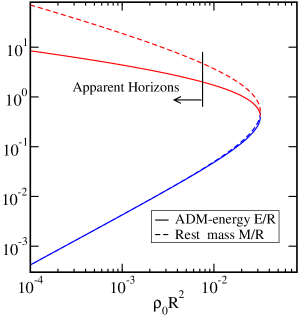
Figure 1: ADM-energy and rest mass as function of $\rho_{0}R^{2}$ for the constant density star of Section III.1.

Next we consider the rest mass $M$ of the star, which is given by

$$M =\int_{r<R}\rho_{0}\sqrt{g}dV=\int_{0}^{R}\rho_{0}\psi^{6}\,4\pi r^{2}\,dr$$

$$=\frac{3}{4\alpha^{5}}\left[\alpha-\alpha^{5}+(1+\alpha^{2})^{3}\arctan(\alpha^{-1})\right]R,$$ (18)

where we have used Eq. (14) to eliminate $\rho_{0}$. This expression has the limiting values

$$M \approx\frac{3\pi}{\alpha^{5}}R \mbox{for }\alpha\to 0,$$ (19)

$$M \approx\frac{2}{\alpha^{2}}R \mbox{for }\alpha\to\infty.$$ (20)

The weak-field limit $\alpha\to\infty$ corresponds to the limit in which the star has vanishing mass, whereas the strong-field limit $\alpha\to 0$ results in a star with unbounded mass, even though the density itself approaches zero. This behavior is caused by the fact that the conformal factor, and hence the proper volume inside the stellar radius $R$ diverges more rapidly than the rate at which the density $\rho_{0}$ vanishes.

We point out that for all $\alpha>0$ we have $E<M$, so that the star has negative binding energy as expected. In the Newtonian limit $\alpha\to\infty$ we recover the Newtonian binding energy,

$$E-M\approx-\frac{12}{5\alpha^{4}}R\approx-\frac{3}{5}\frac{M^{2}}{R},$$ (21)

where we have used Eq. (20) in the second step.

Finally, we locate the apparent horizons in this family of initial data sets. For a time-symmetric hypersurface, apparent horizons coincide with maximal surfaces, which in spherical symmetry and conformal flatness are given by the roots of

$$\frac{\partial\psi}{\partial r}+\frac{\psi}{2r}=0.$$ (22)

For $\alpha\!>\!1$, no roots to this equation exist, so that the initial data surface does not contain an apparent horizon. For $\alpha<1$, two roots exist, one in the interior of the star at $r=\alpha R$, and one in the exterior at $r=R/\alpha^{2}$. The latter one is the outermost extremal surface, which is the apparent horizon. Both extremal surfaces merge on the surface of the star for $\alpha=1$. The density, ADM-energy and rest mass at formation of the apparent horizon are $\rho_{0}|_{\alpha=1}=3/(128\pi R^{2})\approx 0.0075R^{-2}$, $E=2R$, and $M|_{\alpha=1}=3\pi R/2\approx 4.71R$.

We now turn our attention to the critical point. Around its maximum $f(\alpha)$ behaves like a parabola, therefore

$$\alpha-\alpha_{c}\propto\pm(\rho_{c}-\rho_{0})^{1/2}.$$ (23)

Energy and mass at the critical point are

$$E_{c} =\frac{2}{5}R,$$ (24)

$$M_{c} =\frac{18}{125}\left(9\sqrt{5}\arctan(1/\sqrt{5})-5\right)R\approx 0.499R,$$ (25)

respectively. Since $\partial E/\partial\alpha\neq 0$ there, the energy also changes parabolically with $\rho_{0}$,

$$E-E_{c}\;\propto\;\alpha-\alpha_{c}\;\propto\;\pm(\rho_{c}-\rho_{0})^{1/2}.$$ (26)

This parabolic behavior is apparent in Fig. 1.

At the critical point the local uniqueness of solutions must break down, since the two branches meet there. For this to happen, the linearized operator must have a non-trivial solution at the critical point. The linearization of Eq. (7) reads

$$\nabla^{2}\delta\psi+10\pi\rho_{0}\psi^{4}\,\delta\psi=0,$$ (27a)

with boundary conditions

$$\frac{\partial\delta\psi}{\partial r}=0, \qquad r=0$$ (27b)

$$\delta\psi\to 0, \qquad r\to\infty.$$ (27c)

We will now construct all solutions of Eq. (27). While doing so, we consider $\rho_{0}$ as given and fixed. If $\delta\psi=0$ is the only solution, then the kernel of this equation is trivial, and solutions to the non-linear equation (7) are locally unique. As just argued, at the critical point this will not be the case, and there must be a non-zero solution of Eq. (27). As it turns out, we can construct this solution analytically.

The key to solving Eq. (27) are again the Sobolev functions $u_{\alpha}$. Recall that $\psi=Cu_{\alpha}$ satisfies Eq. (7) in the interior of the star for any value of $\alpha$. We can therefore take the derivative of Eq. (7) with respect to $\alpha$ and find

$$\nabla^{2}\frac{\partial u_{\alpha}}{\partial\alpha}+10\pi\rho_{0}C^{4}u_{\alpha}^{4}\frac{\partial u_{\alpha}}{\partial\alpha}=0.$$ (28)

Choosing $\alpha$ to be a solution of (14), so that it is consistent with $\rho_{0}$, we can identify $C^{4}u_{\alpha}^{4}=\psi^{4}$, and Eq. (28) reduces to Eq. (27a). Consequently, any function $A\partial u_{\alpha}/\partial\alpha$, with $\alpha$ given by (14) and $A$ an arbitrary constant, satisfies Eq. (27a). This forms a one-parameter family of functions, all of which automatically satisfy the differential equation Eqs. (27a) and the boundary condition (27b) in the interior.

Solutions $\delta\psi$ in the exterior must satisfy the Laplace equation and the outer boundary condition (27c), i.e. they must take the form $B/r$ for some constant $B$. Since this is a one-parameter family of solutions, we have found all solutions to Eqs. (27a) and (27c) in the exterior.

To find a global solution $\delta\psi$ we now have to find constants $A$ and $B$ so that the interior solution $A\partial u_{\alpha}/\partial\alpha$ matches the exterior solution $B/r$ continuously in both the functions and their first derivatives at the stellar radius $r=R$. As expected, non-trivial solutions with non-zero $A$ and $B$ exist only at the critical point $\alpha=\alpha_{c}$. There, the solution $\delta\psi$ takes the form

$$\delta\psi_{c}(r)\propto\left\{\begin{aligned} &\frac{5R^{2}-r^{2}}{(r^{2}+5R^{2})^{3/2}},&r<R\\ &\frac{4}{6^{3/2}r},&r>R\end{aligned}\right.$$ (29)

and it is easy to verify that it indeed satisfies Eq. (27) at the critical point.

III.2 Results for general $\rho\geq 0$

A fully worked out example like the constant density star presented above is very instructive. However, the example itself does not provide any indication whether its behavior is generic. In this Section we prove theorems valid for general $\rho\geq 0$ with compact support, indicating that the behavior found for the constant density star is indeed generic for the Hamiltonian constraint with unscaled matter density. We will first show that for sufficiently “large” matter-densities $\rho$, no solution exists. We will then consider the critical point and show that if a critical point exists, the solution must vary parabolically close to it, as did the constant density star, cf. Eq. (23). Finally, we will prove a result which was stated above to show that all solutions to the constant density star have been found: If two functions each satisfying Eqs. (7a) and (7b) have the same value at the origin, then they are identical.

We start with some preliminaries. Rewriting the Laplacian in Eq. (7) we find

$$\left(\psi+r\psi^{\prime}\right)^{\prime}=-2\pi r\rho\psi^{5}\leq 0.$$ (30)

Therefore the combination $\psi+r\psi^{\prime}$ is monotonically decreasing and bounded from below by its asymptotic value for large $r$,

$$\psi+r\psi^{\prime}\geq 1.$$ (31)

Furthermore, integrating Eq. (7) over a sphere of radius $R$ we find

$$4\pi R^{2}\;\psi^{\prime}(R)=-2\pi\int_{R}\rho\psi^{5}dV.$$ (32)

Since $\rho\geq 0$ and $\psi>0$ we have $\psi^{\prime}\leq 0$, so that $\psi$ is a decreasing function of radius, which is bounded from below by its asymptotic value, $\psi\geq 1$.

We can now show that for sufficiently large $\rho$ Eq. (7) does not admit strictly positive solutions $\psi$. Solving Eq. (32) for $\psi^{\prime}(R)$ and substituting into Eq. (31) we find

$$2R\big{[}\psi(R)-1\big{]}\geq\int_{R}\rho\,\psi^{5}\,dV\geq\psi(R)^{5-k}\int_{R}\psi^{k}\rho\,dV,$$ (33)

for any $k\leq 5$, where the last inequality follows from $\psi^{\prime}\leq 0$. Rearranging terms we obtain

$$\frac{1}{R}\int_{R}\psi^{k}\rho\,dV\leq 2\frac{\psi(R)-1}{\psi(R)^{5-k}}.$$ (34)

The right hand side of this inequality is bounded independently of the value of $\psi(R)$ by the biggest value of the function

$$g_{k}(x)=2\frac{x-1}{x^{5-k}}$$ (35)

for $x\geq 1$. For $k\leq 4$, this function is bounded by

$$g_{k}(x)\leq C_{k}\equiv 2\frac{(4-k)^{4-k}}{(5-k)^{5-k}},$$ (36)

so that any solution $\psi$ satisfies the integral bounds

$$\frac{1}{R}\int_{R}\psi^{k}\rho\,dV\leq C_{k}$$ (37)

for any $k\leq 4$. For a given $k$, the bound $C_{k}$ is independent of $R$. For positive $k$, $0<k\leq 4$, this inequality constrains how large solutions can be. For example,

$$C_{4}\geq\frac{1}{R}\int_{R}\psi^{4}\rho\,dV\geq\frac{\psi(R)^{4}}{R}\int_{R}\rho\,dV$$ (38)

implies

$$\psi(R)\leq C_{4}^{1/4}\left(\frac{1}{R}\int_{R}\rho\,dV\right)^{-1/4},$$ (39)

which is a bound of how quickly the “upper” branch can diverge as $\rho\to 0$.

For $k=0$, the inequality (37) becomes independent of $\psi$: If a solution $\psi$ exists for a certain $\rho$, then

$$\frac{1}{R}\int_{R}\rho\,dV\leq 2\frac{4^{4}}{5^{5}}\approx 0.163.$$ (40)

Equation (40) holds for any $R$ for any strictly positive solution of Eq. (7), therefore if a density distribution $\rho(r)$ satisfies

$$m(R)\equiv\int_{R}\rho\,dV>2\frac{4^{4}}{5^{5}}R$$ (41)

even for one $R$, then no regular solution to the Hamiltonian constraint Eq. (7) exists for this density.

For the constant density star, $m(r)$ is largest at the surface of the star, $r=R$, where

$$m(R)=\rho_{0}\int_{R}4\pi r^{2}dr=\frac{4\pi}{3}\rho_{0}R^{3}.$$ (42)

Equation (41) then gives the necessary bound $\rho_{0}\lesssim 0.0389/R^{2}$ for the existence of solutions. Comparison with the exact critical density $\rho_{c}=0.0320/R^{2}$ from Eq. (16) reveals that the upper bound of the theorem is only 20 per cent larger than the exact critical density (see also Fig. 1).

Let us now examine the character of the critical point. We take a smooth sequence of non-negative densities, $\rho_{\gamma}$, such that $\rho\equiv 0$ when $\gamma=0$. We then look for a smooth sequence of solutions $\psi_{\gamma}$ to Eq. (7) with the density $\rho$ given by $\rho_{\gamma}$, starting from $\psi\equiv 1$ at $\gamma=0$. The Implicit Function Theorem tells us that as long as the linearized equation, Eq. (27),

$$\nabla^{2}\delta\psi+10\pi\rho_{\gamma}\psi_{\gamma}^{4}\,\delta\psi=0,$$ (43a)

with boundary conditions

$$\frac{\partial\delta\psi}{\partial r}=0, \qquad r=0$$ (43b)

$$\delta\psi\to 0, \qquad r\to\infty.$$ (43c)

has no non-trivial solution, then the full nonlinear equation

$$\nabla^{2}\psi_{\gamma}+2\pi\rho_{\gamma}\psi_{\gamma}^{5}=0,\\$$ (44a)

with boundary conditions

$$\frac{\partial\psi}{\partial r}=0, \qquad r=0,$$ (44b)

$$\psi_{\gamma}\to 1, \qquad r\to\infty,$$ (44c)

has a regular solution which changes smoothly as a function of $\gamma$.

The obvious question to ask is what happens if the sequence approaches the point where the first kernel of Eq. (43) appears. Let us assume this happens at $\gamma_{0}$. The trick is to consider the limiting process rather than the limit point itself. We know that when $\gamma=\gamma_{0}$ the equation

$$\nabla^{2}\theta+10\pi\rho_{\gamma_{0}}\psi_{\gamma_{0}}^{4}\theta=0,$$ (45)

has a positive solution $\theta$, going to zero at infinity. This is the ground state of a Schrödinger equation, because it is the first appearance of a kernel, hence it has no nodes, and thus it can be chosen to be everywhere positive.

We now differentiate Eq. (44a) with respect to $\gamma$ (at any $\gamma<\gamma_{0}$ to find

$$\nabla^{2}\frac{d\psi_{\gamma}}{d\gamma}+10\pi\rho_{\gamma}\psi_{\gamma}^{4}\frac{d\psi_{\gamma}}{d\gamma}=-2\pi\frac{d\rho_{\gamma}}{d\gamma}\psi_{\gamma}^{5}.$$ (46)

Multiplying Eq. (45) by $d\psi_{\gamma}/{d\gamma}$, Eq. (46) by $\theta$ and subtracting the results we obtain

$$\nabla\cdot(\frac{d\psi_{\gamma}}{d\gamma} \nabla\theta-\theta\nabla\frac{d\psi_{\gamma}}{d\gamma})=\frac{d\psi_{\gamma}}{d\gamma}\nabla^{2}\theta-\theta\nabla^{2}\frac{d\psi_{\gamma}}{d\gamma}$$

$$= 10\pi(\rho_{\gamma}\psi_{\gamma}^{4}-\rho_{\gamma_{0}}\psi_{\gamma_{0}}^{4})\frac{d\psi_{\gamma}}{d\gamma}\theta+2\pi\frac{d\rho_{\gamma}}{d\gamma}\psi_{\gamma}^{5}\theta.$$ (47)

Next we wish to integrate this equation over the whole space. Let us assume that $\rho_{\gamma}$ has compact support, or, at least, falls off rapidly at infinity. Both $\theta$ and $d\psi_{\gamma}/d\gamma$ fall off at infinity like $1/r$ and their first derivatives fall off like $1/r^{2}$. This means that the total divergence upon integration becomes a surface term, and the integrand falls off like $1/r^{3}$. Therefore the integral vanishes. We get

$$5\int(\rho_{\gamma}\psi_{\gamma}^{4}-\rho_{\gamma_{0}}\psi_{\gamma_{0}}^{4})\frac{d\psi_{\gamma}}{d\gamma}\,\theta\,dV+\int\frac{d\rho_{\gamma}}{d\gamma}\psi_{\gamma}^{5}\,\theta\,dV=0.$$ (48)

Consider this in the limit as $\gamma\rightarrow\gamma_{0}$. The second term tends to the constant

$${\cal I}\equiv\int\left.\frac{d\rho_{\gamma}}{d\gamma}\right|_{\gamma_{0}}\!\psi^{5}_{\gamma_{0}}\,\theta\,dV.$$ (49)

Note that both $\theta$ and $\psi_{\gamma_{0}}$ depend only on $\rho_{\gamma_{0}}$, and not its derivative. Therefore, changing $\left.d\rho_{\gamma}/d\gamma\right|_{\gamma_{0}}$ via

$$\rho_{\gamma}\to\rho_{\gamma}+v(\gamma-\gamma_{0})$$ (50)

for any function $v(r)$ will change ${\cal I}$ as

$${\cal I}\to{\cal I}+\int v\,\psi^{5}_{\gamma_{0}}\,\theta\,dV.$$ (51)

Clearly, except for special instances, ${\cal I}$ will be non-zero. Let us now assume this generic case, ${\cal I}\neq 0$ . In the limit $\gamma\to\gamma_{0}$, the second term in Eq. (48) becomes the non-zero constant ${\cal I}$, whereas the first term seems to go to zero. This cannot be and thus we are forced to conclude that the limiting process as $\gamma\rightarrow\gamma_{0}$ must be somehow singular.

The only thing that can possibly go bad is that $d\psi_{\gamma}/d\gamma\rightarrow\infty$. Not only has it to blow up, it must do so over an extended region. This is the only way that the integral, in the limit, can go to a nonzero value. Let us assume

$$\frac{d\psi_{\gamma}}{d\gamma}\propto(\gamma_{0}-\gamma)^{p}$$ (52)

for some negative power $p<0$. This implies

$$\psi_{\gamma}-\psi_{\gamma_{0}}\propto(\gamma_{0}-\gamma)^{p+1}.$$ (53)

Consider now the term

$$\rho_{\gamma}\psi_{\gamma}^{4} -\rho_{\gamma_{0}}\psi^{4}_{\gamma_{0}}=\left(\rho_{\gamma}-\rho_{\gamma_{0}}\right)\psi_{\gamma}^{4}$$ (54)

$$+ \rho_{\gamma_{0}}\left(\psi_{\gamma}^{3}+\psi_{\gamma}^{2}\psi_{\gamma_{0}}+\psi^{\gamma}\psi^{2}_{\gamma_{0}}+\psi^{3}_{\gamma_{0}}\right)\left(\psi_{\gamma}-\psi_{\gamma_{0}}\right)$$

in the first integral in Eq. (48). The first term on the right hand side scales as $\gamma_{0}-\gamma$ as the critical point is approached, whereas the second one scales as $(\gamma-\gamma_{0})^{p+1}$. Because $p+1<1$, the second term dominates, and the full integrand scales as

$$\left(\rho_{\gamma}\psi_{\gamma}^{4}-\rho_{\gamma_{0}}\psi^{4}_{\gamma_{0}}\right)\frac{d\psi_{\gamma}}{d\gamma}\propto(\gamma_{0}-\gamma)^{p+1}(\gamma_{0}-\gamma)^{p}$$ (55)

close to the critical point. In the generic case, the integral has to approach the finite, non-zero value ${\cal I}$ in the limit $\gamma\to\gamma_{0}$, which can only happen if $p=-1/2$. Therefore, the solution must vary parabolically,

$$\psi_{\gamma}-\psi_{\gamma_{0}}\propto\left(\gamma-\gamma_{0}\right)^{1/2}.$$ (56)

This is exactly the behavior we have seen in the constant density star model and also with what Pfeiffer and York Pfeiffer and York  Jr. (2005) observed.

This parabolic nature of solutions near the critical point can be demonstrated explicitly even in the non spherically symmetric case by using Lyapunov-Schmidt techniques Ó Murchadha and Walsh (2006). We conjecture that a second branch of solutions exists beyond the critical point as a consequence of this parabolic behavior. We have seen this explicitly for the constant density stars, and we again refer to Ó Murchadha and Walsh (2006) for a more general treatment.

So far we have shown that there are distributions $\rho(r)$ for which no solutions of Eq. (7) exist, and based on the parabolic nature of the solutions at the critical point we have conjectured that there are distributions for which exactly two solutions exist. We do not know whether this is generic.

Having moved past the first critical point, an open question is whether another critical point is reached. Immediately past the first critical point, $\rho$ does not change, but the conformal factor increases. In the language of the Schrödinger equation this means that the potential deepens and the zero-energy ground state becomes a bound state with negative energy. As one moves away from the critical point along the upper branch one is moving ‘back’ toward smaller $\gamma$, and so we expect $\rho_{\gamma}$ to decrease while $\psi$ continues to increase. One could have that $\rho\psi^{5}$ increases enough that the first excited state appears with zero energy, or that $\rho\psi^{5}$ decreases again so that the ground state becomes a zero energy state again. In either case, the system reaches another critical point and the solution curve may turn again. Alternatively, $\rho_{\gamma}\psi_{\gamma}^{5}$ may be such that neither of these two cases happens and the solution continues on all the way to $\gamma=0$. This last alternative occurs for the constant density star, as we have shown by explicit calculation; however, we do not know whether this behavior is generic.

Finally, we show that if we have two positive solutions $\psi_{1}$ and $\psi_{2}$ to Eq. (7) whose maxima agree, then they are identical. To prove this we first note that the maxima of both must occur at $r=0$. The maximum principle tells us that there cannot be a positive minimum, therefore there can only be one maximum, and therefore it must occur at the origin. Therefore at $r=0$, the two functions $\psi_{1}$ and $\psi_{2}$ agree, their first derivatives both vanish, and the second derivatives are equal (from Eq.(7)). By differentiating Eq.(7), one can show that all the derivatives of the two functions agree at $r=0$. If the functions were analytic, we were done. However, there is no reason to expect that this be true. We need a more subtle argument.

Track $\psi_{1}$ and $\psi_{2}$ as they move out from the origin. If they remain the same all the way to infinity, we are done. Instead, let us assume that at some point $\psi_{1}>\psi_{2}$. Therefore we must encounter a region in which $d(\psi_{1}-\psi_{2})/dr>0$ and $\psi_{1}-\psi_{2}>0$ and inside this region $\psi_{1}\geq\psi_{2}$. Take a point in this region, call it $R_{0}$. Consider the equations satisfied by $\psi_{1}$ and $\psi_{2}$, subtract one from the other and integrate over the ball of radius $R_{0}$. We get

$$\int_{R_{0}}\nabla^{2}(\psi_{1}-\psi_{2})dV+2\pi\int_{R_{0}}\rho(\psi_{1}^{5}-\psi_{2}^{5})dV=0.$$ (57)

The Laplacian becomes a boundary term, which is positive, because the gradient of the difference is positive at $R_{0}$, while the bulk term is also non-negative. This cannot be, so therefore the initial assumption that the functions are different must be incorrect.

IV Summary and Discussion

In this paper we investigate the reason for non-uniqueness in the extended conformal thin sandwich equations Pfeiffer and York  Jr. (2005). We argue that a term with the “wrong sign” in the elliptic equation determining the lapse, Eq. (6), is the cause for non-uniqueness. The sign of this particular term is such that the maximum principle cannot be applied to prove local uniqueness of solutions. We support our claim by examining a simpler equation having a term with an analogous “wrong sign”, namely the the Hamiltonian constraint with unscaled York, Jr. (1979) matter source $\rho$ (cf. Eq. (1)). Specializing to constant density stars we construct analytical solutions. We find two branches of solutions – a weak-field and a strong-field branch – with properties that are remarkably similar to those found by PY.

We comment briefly that solutions to the original conformal thin-sandwich decomposition, consisting of the Hamiltonian constraint (1) and the momentum constraint (4) only, are unique Cantor (1977); Cantor and Brill (1981); York, Jr. (1999); Bartnik and Isenberg (2004); Maxwell (2005); Pfeiffer and York  Jr. (2005). PY found multiple solutions only for the extended conformal thin-sandwich decomposition, which includes the lapse equation (5) in addition to the two constraints. This, too, suggests that the non-uniqueness is caused by the lapse equation, in accordance with our findings.

Our findings are certainly relevant for numerical work: If one wants to solve the extended conformal thin sandwich equations, then apparently, the possibility of finding two solutions is unavoidable. Whether this will pose a problem for numerical work is less clear. Sufficiently far away from the critical point, the solutions along the upper and lower branch are significantly different, and it should be obvious which solution is desired (generally the “lower” one, which reduces to flat space for trivial free data). Many different researchers have solved the extended conformal thin sandwich equations without problems Baumgarte et al. (1997); Bonazzola et al. (1999); Uryū and Eriguchi (2000); Gourgoulhon et al. (2001, 2002); Grandclément et al. (2002); Yo et al. (2004); Cook and Pfeiffer (2004); Caudill et al. (2006); Baumgarte et al. (2004); K. Taniguchi, T. W. Baumgarte, J. A. Faber and S. L. Shapiro (2005) and have obtained a solution with satisfactory properties. However, past success is no guarantee for future success, and for choices of free data which may be interesting in the future, non-uniqueness issues could very well arise, especially if one is interested in solutions which happen to be “close” to the critical point. Indeed, in constrained evolutions schemes, which solve elliptic equations similar to the extended conformal thin sandwich equations, it was reported that the elliptic solver failed to converge in near-critical collapse of Brill waves Choptuik et al. (2003); Rinne (2005). It was further argued that this failure related to the “wrong sign” in a term of the maximum slicing condition Rinne (2005); Rinne and Stewart (2005). How precisely a numerical code behaves in such cases depends very sensitively on its implementation. Some algorithms may not converge at all, like the multi-grid schemes in Choptuik et al. (2003); Rinne (2005), while other algorithms may converge to one of the two solutions (e.g. the Newton-Raphson method used in PY; cf. Pfeiffer et al. (2003)). In the former case it may be difficult to ascertain whether failure of the numerical method is indeed due to non-uniqueness properties of the underlying analytic problem (rather than a bug), whereas in the latter case one is faced with the question of which of the two solutions one wants, and how to ensure convergence toward the desired solution.