Spectral Representations of Neutron-Star Equations of State
Abstract
Methods are developed for constructing spectral representations of cold (barotropic) neutron-star equations of state. These representations are faithful in the sense that every physical equation of state has a representation of this type, and conversely every such representation satisfies the minimal thermodynamic stability criteria required of any physical equation of state. These spectral representations are also efficient, in the sense that only a few spectral coefficients are generally required to represent neutron-star equations of state quiet accurately. This accuracy and efficiency is illustrated by constructing spectral fits to a large collection of “realistic” neutron-star equations of state.
I Introduction
The gravitational field of a neutron star compresses the material in its core to densities that exceed those inside normal atomic nuclei. The resulting matter is a mixture of free baryons (neutrons and protons), leptons (electrons and muons), and likely also smaller fractions of hyperons, mesons, or perhaps even free quarks. The basic thermodynamic relationship between the total energy density , and the pressure of this material is called its equation of state, , and is determined by the complicated micro-physical interactions between the various particle species present in the mixture Shapiro and Teukolsky (1983).
In addition to its dependence on the pressure, the energy density of a mixture also depends typically on the temperature and other quantities like the relative abundances of the different particle species. Thus there is no guarantee that a simple barotropic form, , applies to any, let alone universally to all, neutron-star matter. Yet there is reason to expect that a universal barotropic form might be an excellent approximation. Neutron stars are born when the cores of massive stars (and perhaps white dwarfs) become unstable and undergo gravitational collapse. Compression heats the material as it collapses, to temperatures that exceed the binding energies of all atomic nuclei. Neutron-star matter always begins therefore as a very hot plasma of free baryons and leptons, etc. This material is expected to evolve quickly to the lowest available energy state as it cools by neutrino and photon emission, and this fixes the relative abundances of the various particle species. The thermal energies of the particles fall rapidly below their Fermi levels, so the thermal contribution to the energy rapidly becomes negligible. The matter therefore is expected to evolve on a very short time scale to a state that is well described by a temperature independent barotropic equation of state. This paper develops more efficient ways to represent equations of state of this type.
The matter densities in the cores of neutron stars are well beyond the reach of current laboratory experiments. Heavy-ion scattering (including most recently those conducted at RHIC and LHC) provides a wealth of information about the interactions among the various particles expected to make up neutron-star matter. Unfortunately those experiments bear only indirectly on the properties of the equilibrium ground state, because the effective temperature of the nuclear matter in the experiments is quite high. Little insight is provided therefore into effects, like complicated many body interactions, that might play a role only in states with low temperature and high density and pressure.
There has also been a significant effort over the past several decades to understand this material from a theoretical perspective: hundreds of papers devoted to modeling neutron-star matter have appeared in the literature. But the properties of this material are far outside the realm where the usual arsenal of theoretical tools were designed to work reliably, so it is not surprising that there is no consensus among theoreticians yet on the neutron-star equation of state. For example, the current models’ predictions of the pressure at a given density still vary by about an order of magnitude Read et al. (2009).
Direct observations of neutron stars may be the most promising approach to understanding the properties of high-density nuclear matter. It is well known that the equation of state along with the gravitational field equations determine the observable macroscopic properties of neutron stars Oppenheimer and Volkoff (1939), and conversely that a complete knowledge of an appropriate set of macroscopic properties (e.g. masses and radii) determines the equation of state Lindblom (1992). Studies of neutron-star models show that their macroscopic properties, like their masses and radii, vary widely even within the current “realistic” class of equations of state Arnett and Bowers (1977); Read et al. (2009). So it has long been recognized that accurate observations of the macroscopic properties of neutron stars will provide significant constraints on the nuclear equation of state. Unfortunately the needed observations are quite difficult to make. Masses of several dozen neutron stars have now been measured fairly accurately (see e.g. Ref. Lattimer and Prakash (2007)), and these observations have ruled out large classes of very “soft” equation of state models. Only a few radius measurements have been made however Steiner et al. (2010), and these are not reliable and accurate enough yet to make solid quantitative measurements of the equation of state itself possible.
There is reason to hope that more abundant and accurate measurements of both neutron-star masses and radii will become available, however. When the first accurate measurements are made, they are not likely to be numerous and accurate enough to determine the entire high density portion of the neutron-star equation of state. Various attempts have been made, therefore, to find representations of equations of state that make their essential features depend on just a few parameters. One approach is to use the parameters that characterize the nuclear interaction models as a way to parametrize the equations of state constructed from them. These might include a number of micro-physical parameters like the bulk nucleon incompressibility and symmetry energy parameters in models of the nucleon interaction potential Prakash et al. (1988), or the coupling constants and mixing angles in effective mean field theory descriptions Glendenning (1985). Comparing the masses and radii of neutron stars based on these model equations of state should fix the values of the unknown nuclear interaction model parameters. This approach would clearly be ideal if a reliable and accurate micro-physical model of neutron-star matter were known. Unfortunately there is no consensus that any of the existing nuclear-matter models are good enough yet to describe neutron-star matter accurately and reliably.
Another approach is to construct purely empirical fits rather than micro-physics based models of the equation of state. The first attempts to do this Lindblom (1992); Vuille (1995) approximated the high density part of the equation of state as a simple polytrope, i.e., an equation of state in which the pressure is proportional to a power of the density.111The term relativistic polytrope is most commonly used for equations of state that satisfy , where is the conserved rest-mass density and is the (constant) adiabatic index. It is also used (less commonly) for those satisfying where is the total energy density and is a constant. The two definitions agree in the Newtonian limit. These first simple fits were shown to reproduce the central pressures and densities of neutron-star models based on “realistic” equations of state with about 15% accuracy Lindblom (1992). This type of approximation can be improved by dividing the relevant range of pressures into a number of intervals, , and fitting a different polytrope to the equation of state in each interval. Any level of accuracy can then be achieved by using a sufficiently large number of intervals. A number of authors have proposed using piecewise polytropes to approximate the high density part of the neutron-star equation of state Vuille (1995); Vuille and Ipser (1999); Read et al. (2009), and these approximations turn out to be quite efficient. Fits of the high density parts of “realistic” neutron-star equations of state have been shown to achieve accuracies of a few percent for piecewise polytropes with only a small number of free parameters Vuille (1995); Vuille and Ipser (1999); Read et al. (2009). The most extensive study to date uses fits with four free parameters that give average errors of only a few percent for 34 realistic equations of state Read et al. (2009). Other types of empirical fits to neutron-star equations of state have also been reported in the literature Haensel and Potekhin (2004); Shibata et al. (2005); Shibata and Taniguchi (2006); Zdunik et al. (2006). These provide high accuracy approximations of particular realistic equations of state (generally using fifteen to twenty parameters to do this), and do not appear to have been intended as efficient ways to model large classes of equations of state.
This paper continues the effort to construct efficient empirical representations of “realistic” neutron-star equations of state. New methods are described here for constructing parametric representations based on spectral fits. Spectral representations are generalizations of the Fourier series used to represent periodic functions. It is shown in Sec. II that spectral representations can be constructed that are faithful, in the sense that every physical equation of state has such a representation and conversely that every such representation satisfies the basic thermodynamic stability conditions required of any equation of state. It is also shown in Sec. III that these spectral representations do a good job of representing the currently available “realistic” neutron-star equations of state. A suitably constructed two-parameter spectral representation is shown to be about as accurate as the most carefully studied four-parameter polytrope fits Read et al. (2009). For smooth equations of state, the errors in the spectral fits decrease exponentially as the number of parameters is increased, while piecewise polytrope fits generally decrease only quadratically. These spectral fits make it possible therefore to provide very accurate representations of the neutron-star equation of state using only a small number parameters. They should provide an important new tool for extracting the high density equation of state from neutron-star observations.
II Spectral Representations of the Equation of State
Any equation of state, , can be represented in a “spectral” expansion, as linear combinations of basis functions :
| (1) |
Any complete set of functions, such as the Fourier basis functions or the Chebyshev polynomials, could be used as the in these expansions. Equations of state are determined in such representations by their spectral coefficients, . Truncated versions of these expansions, in which only a finite number of terms are kept, provide approximate parametric representations of arbitrary equations of state: .
Physical equations of state must be non-negative, , and monotonically increasing functions, , to insure thermodynamic stability. Since almost all functions fail to satisfy these conditions, it follows that almost all choices of spectral coefficients, , in an expansion such as Eq. (1) represent functions that can not be equations of state. Thus the spectral coefficients obtained by fitting to a physical equations of state are likely to produce a representation that violates basic thermodynamic stability. So unfortunately, representing an equation of state with a straightforward spectral expansion is not particularly useful.
Instead, faithful representations are needed: ones that ensure the positivity and monotonicity conditions for every choice of spectral coefficients. Methods of constructing faithful representations of the equation of state are presented in the following sections. Spectral representations of the standard form of the equation of state, in which the energy density is expressed as a function of the pressure , are presented in Sec. II.1. For some applications it is more convenient to express the equation of state in terms of the relativistic enthalpy . Spectral representations of these enthalpy based forms are given in Sec. II.2.
II.1 Pressure Based Forms
An equation of state determines, and is determined by (up to an integration constant), the adiabatic index , defined by
| (2) |
Given , the equation of state is determined simply by integrating the first-order ordinary differential equation,
| (3) |
The adiabatic index must be positive to ensure thermodynamic stability, but it need not be monotonic. Thus a larger class of functions represent possible physical adiabatic indices, and this makes it easier to represent equations of state through spectral expansions of . In particular, every physical equation of state can be represented by the following spectral expansion of the adiabatic index :
| (4) |
Conversely, every choice of (for which the series in this expansion converges) results in a positive adiabatic index, and thus an equation of state from Eq. (3), that satisfies the positivity and thermodynamic stability conditions. So this representation is faithful in the sense defined in Sec. II.
The construction of an explicit spectral representation of the equation of state requires a choice for the basis functions . To that end, it is useful to define a dimensionless logarithmic pressure variable:
| (5) |
The constant is a scale factor, chosen here to be the minimum value of the pressure, , in the domain where the spectral expansions are to be used. The following expansion of the adiabatic index is found to be useful and effective,
| (6) |
One advantage of this simple power-law basis is that the lowest order spectral coefficients have fairly simple physical interpretations. For example the lowest order coefficient, , is determined by the adiabatic index evaluated at the reference pressure: . Similarly, the next coefficient, , determines the behavior of the adiabatic index, for pressures near , i.e. for .
The power law basis, , has the advantage of simplicity. While it might be advantageous to choose another basis like the Chebyshev polynomials for some purposes, these advantages can only be fully exploited by using a knowledge of the exact range, , and re-scaling in the optimal way. The additional information, like for example, needed to do that will not be available a priori for the real neutron-star equation of state. So here the simple power law basis is used, and fortunately this choice seems to work quite well.
Given an adiabatic index, , it is straightforward to determine the equation of state, , by integrating the ordinary differential equation, Eq. (3). The solutions and hence the equation of state can be reduced to quadratures:
| (7) |
where is defined as
| (8) |
and where is the constant of integration needed to fix the solution. This is fixed in the fits performed in Sec. III by matching to a low density equation of state at the pressure, (i.e. at ), chosen to be a point somewhat below nuclear density.
The quadratures indicated in Eq. (7) can not be done analytically for the expansion given in Eq. (6), so an explicit analytic expression for the equation of state is not available in this case. However, the integrands in these quadratures are analytic functions that can be integrated numerically very accurately and efficiently. Using Gaussian quadrature for example, double precision accuracy can be achieved using about 10 points for each integral. So there is very little practical difference between having an explicit analytic expression for the equation of state, and the expression in Eq. (7) in terms of quadratures of explicit analytic functions.
It might be advantageous in some situations to construct spectral expansions for the equation of state using thermodynamic quantities other than . For example, the adiabatic sound speed, , defined by
| (9) |
(where is the speed of light) could be used to obtain the equation of state by integrating the simple ordinary differential equation,
| (10) |
The thermodynamic stability condition, , could be enforced in this case by constructing the following spectral expansion,
| (11) |
Alternatively, it might be desirable to enforce both the thermodynamic stability condition and the “causality” conditions,222The condition only represents a true causality condition if the equation of state describes both the time dependent and the equilibrium properties of the material. In neutron-star matter, various strong and weak nuclear interactions determine the relative abundances of the various particle species in the equilibrium state. Thus evaluated for the equilibrium equation of state only describes the sound propagation speed for low enough frequency waves that the material remains continuously in equilibrium. The condition may or may not represent a causality constraint therefore on sound waves with short enough wavelengths to be physically relevant in neutron stars. , by constructing the spectral expansion in the following way,
| (12) |
For the remainder of this paper, spectral representations of the equation of state will be based on the familiar adiabatic index . The discussion in Sec. III shows that is a reasonably slowly varying function for “realistic” neutron-star equations of state, which can be represented fairly accurately using expansions having only a few terms. Using for these expansions also allows us to make straightforward comparisons with published piecewise-polytrope approximations to the equation of state Read et al. (2009). The accuracy and efficiency of these expansions in representing “realistic” neutron-star equations of state is explored in Sec. III.
II.2 Enthalpy Based Forms
The spectral expansions of the standard representation of equation of state, , should be quite useful for many applications. For some applications, however, the standard representation, , is not ideal. For example, a useful form of the relativistic stellar structure equations Lindblom (1992) requires the equation of state to be expressed in terms of the relativistic enthalpy, . For applications such as this, must be re-written as a pair of equations and , where is defined as
| (13) |
The needed expressions, and , are constructed by inverting from Eq. (13) to obtain , and composing the result with the standard equation of state, , to obtain .
The transformations needed to construct and are difficult to perform numerically in an efficient and accurate way. Therefore it may be preferable to construct a spectral expansion of the equation of state based directly on . This can be done using the methods described above for the standard representation. To do this a spectral expansion of the adiabatic index, considered now as a function of the enthalpy , must be defined. The scaled enthalpy variable , is found to be useful, where is the lower bound on the enthalpy, , in the domain where the spectral expansions are constructed. The expression for given in Eq. (6) then provides a useful expansion for :
| (14) |
Next, the functions and are defined by the system of ordinary differential equations,
| (15) | |||||
| (16) |
that follow from the definitions of , Eq. (13), and , Eq. (2). The general solution to these equations can be reduced to quadrature:
| (17) | |||||
| (18) |
where is defined as,
| (19) |
The constants and are defined by and respectively. While these quadratures can not be done analytically for the spectral expansion defined in Eqs. (14), they can be done numerically very efficiently and accurately using Gaussian quadrature, as in the standard equation of state case.
III Spectral Fits to Realistic Equations of State
The discussion in Sec. II shows how any equation of state can be represented by spectral expansions of the adiabatic index, like the one given in Eq. (6). When these expansions are truncated, keeping only a finite number of terms, they produce fits to the equation of state, that are expected to converge to the exact as the number of terms in the expansion increases. In analogy with Fourier series, the rate of convergence for these fits should be exponential for smooth equations of state, and power law for less than smooth cases. The smoothness of an equation of state is determined by the details of the micro-physics that controls the properties of the material. The convergence rate of an expansion will be reduced therefore, from exponential to power law, when phase transitions or other non-smooth transitions are present. The number of terms required to achieve a certain level of accuracy in , therefore, will depend on the smoothness and variability of the adiabatic index , and the suitability of the chosen spectral basis functions .
The accuracy and practicality of spectral expansions for two forms of the equation of state, and , are evaluated in this section by constructing fits to 34 “realistic” neutron-star equations of state. These spectral fits are based on finite spectral expansions of and respectively. The equations of state used for these fits are the same as those used by Read, Lackey, Owen and Friedman Read et al. (2009) in their study of piecewise-polytrope approximations. These realistic equations of state are based on a variety of different models for the composition of neutron-star matter, and a variety of different models for the interactions between the particle species present in the model material. Descriptions of these realistic equation of state models, and references to the original publications on each of these equations of state are given in Ref. Read et al. (2009), and are not repeated here. The individual equations of state are referred to here using the abbreviations used in Ref. Read et al. (2009), e.g. PAL6, APR1, BGN1H1, etc. The list of these equations of state are given in the first column of Table III of Ref. Read et al. (2009), and the first columns of Tables 1 and 2 in this paper.
| EOS | ||||||||||||
|---|---|---|---|---|---|---|---|---|---|---|---|---|
| PAL6 | 0.0076 | 0.0025 | 0.0014 | 0.0005 | 0.0001 | 0.8622 | -0.0677 | 0.0181 | -0.0017 | 5.79 | ||
| SLy | 0.0208 | 0.0076 | 0.0028 | 0.0010 | 0.0002 | 0.9865 | 0.1110 | -0.0301 | 0.0022 | 6.73 | ||
| AP1 | 0.0831 | 0.0552 | 0.0199 | 0.0098 | 0.0029 | 0.4132 | 0.5594 | -0.1270 | 0.0085 | 7.38 | ||
| AP2 | 0.0411 | 0.0236 | 0.0091 | 0.0033 | 0.0017 | 0.7065 | 0.2866 | -0.0659 | 0.0047 | 7.27 | ||
| AP3 | 0.0352 | 0.0204 | 0.0026 | 0.0011 | 0.0009 | 0.9214 | 0.2097 | -0.0383 | 0.0019 | 6.87 | ||
| AP4 | 0.0273 | 0.0194 | 0.0016 | 0.0015 | 0.0013 | 0.8651 | 0.1548 | -0.0151 | -0.0002 | 7.04 | ||
| FPS | 0.0120 | 0.0045 | 0.0037 | 0.0034 | 0.0021 | 1.1561 | -0.0468 | 0.0081 | -0.0010 | 7.04 | ||
| WFF1 | 0.0320 | 0.0387 | 0.0067 | 0.0066 | 0.0062 | 0.6785 | 0.2626 | -0.0215 | -0.0008 | 7.48 | ||
| WFF2 | 0.0342 | 0.0200 | 0.0077 | 0.0051 | 0.0041 | 0.8079 | 0.2680 | -0.0558 | 0.0039 | 7.25 | ||
| WFF3 | 0.0314 | 0.0081 | 0.0081 | 0.0060 | 0.0059 | 1.4126 | -0.1797 | 0.0389 | -0.0035 | 7.32 | ||
| BBB2 | 0.1016 | 0.0283 | 0.0238 | 0.0167 | 0.0042 | 0.7390 | 0.4555 | -0.1406 | 0.0121 | 6.97 | ||
| BPAL12 | 0.0739 | 0.0138 | 0.0086 | 0.0043 | 0.0018 | 1.1081 | -0.3078 | 0.0891 | -0.0081 | 6.08 | ||
| ENG | 0.0527 | 0.0181 | 0.0168 | 0.0138 | 0.0118 | 0.9820 | 0.2716 | -0.0862 | 0.0075 | 6.98 | ||
| MPA1 | 0.0365 | 0.0223 | 0.0022 | 0.0022 | 0.0019 | 1.0215 | 0.1653 | -0.0235 | -0.0004 | 6.63 | ||
| MS1 | 0.0581 | 0.0256 | 0.0052 | 0.0039 | 0.0004 | 0.9189 | 0.1432 | 0.0122 | -0.0094 | 5.05 | ||
| MS2 | 0.0155 | 0.0074 | 0.0013 | 0.0005 | 0.0001 | 0.9598 | -0.0527 | 0.0091 | -0.0035 | 4.77 | ||
| MS1b | 0.0206 | 0.0179 | 0.0058 | 0.0032 | 0.0004 | 1.2132 | -0.0648 | 0.0561 | -0.0111 | 5.40 | ||
| PS | 0.0568 | 0.0566 | 0.0294 | 0.0284 | 0.0182 | 1.3896 | -0.8472 | 0.2636 | -0.0218 | 4.77 | ||
| GS1 | 0.0536 | 0.0762 | 0.0385 | 0.0333 | 0.0265 | 1.8662 | -1.4266 | 0.4450 | -0.0389 | 6.28 | ||
| GS2 | 0.0416 | 0.0582 | 0.0427 | 0.0425 | 0.0294 | 1.4580 | -0.7219 | 0.1828 | -0.0117 | 4.99 | ||
| BGN1H1 | 0.0435 | 0.0792 | 0.0460 | 0.0439 | 0.0328 | 1.3450 | -0.0996 | -0.0833 | 0.0161 | 6.40 | ||
| GNH3 | 0.0092 | 0.0130 | 0.0090 | 0.0081 | 0.0057 | 1.0366 | -0.0044 | -0.0440 | 0.0075 | 5.26 | ||
| H1 | 0.0226 | 0.0200 | 0.0117 | 0.0089 | 0.0069 | 1.0653 | 0.0362 | -0.1098 | 0.0179 | 5.04 | ||
| H2 | 0.0300 | 0.0181 | 0.0133 | 0.0072 | 0.0069 | 1.0743 | 0.2250 | -0.2029 | 0.0290 | 4.98 | ||
| H3 | 0.0308 | 0.0130 | 0.0109 | 0.0086 | 0.0066 | 1.1340 | 0.0925 | -0.1303 | 0.0190 | 4.91 | ||
| H4 | 0.0098 | 0.0098 | 0.0097 | 0.0069 | 0.0063 | 1.0526 | 0.1695 | -0.1200 | 0.0150 | 5.21 | ||
| H5 | 0.0214 | 0.0150 | 0.0126 | 0.0054 | 0.0054 | 1.0106 | 0.2765 | -0.2011 | 0.0270 | 5.09 | ||
| H6 | 0.0185 | 0.0137 | 0.0133 | 0.0130 | 0.0100 | 1.0650 | -0.0196 | -0.0474 | 0.0077 | 4.80 | ||
| H7 | 0.0139 | 0.0132 | 0.0103 | 0.0059 | 0.0056 | 0.9582 | 0.1619 | -0.1294 | 0.0177 | 5.22 | ||
| PCL2 | 0.0227 | 0.0252 | 0.0121 | 0.0090 | 0.0075 | 1.0410 | 0.0173 | -0.0904 | 0.0150 | 5.44 | ||
| ALF1 | 0.0947 | 0.0669 | 0.0453 | 0.0369 | 0.0305 | 1.0143 | -0.3102 | 0.1809 | -0.0248 | 6.21 | ||
| ALF2 | 0.0655 | 0.0629 | 0.0450 | 0.0256 | 0.0230 | 0.4613 | 1.5237 | -0.5817 | 0.0571 | 5.79 | ||
| ALF3 | 0.0371 | 0.0355 | 0.0139 | 0.0132 | 0.0131 | 0.8536 | 0.2405 | -0.0743 | 0.0041 | 6.14 | ||
| ALF4 | 0.0453 | 0.0652 | 0.0166 | 0.0089 | 0.0088 | 0.8806 | 0.0656 | 0.0765 | -0.0177 | 5.97 | ||
| Average | 0.0383 | 0.0287 | 0.0149 | 0.0114 | 0.0085 |
Approximate equations of state, , have been constructed for each of the realistic neutron-star equations of state listed in Table 1. These approximations are based on Eq. (7) with determined by the spectral expansion in Eq. (6). The constructed in this way depend on the pressure through the variable , as well as the spectral coefficients : . The optimal choice of spectral coefficients, , is made by minimizing the differences between and the exact for a set of pressures, , from the realistic neutron-star equation of state tables. These differences are measured by constructing the residual:
| (20) |
where the sum is over all the pressures in the tabulated realistic equation of state in the range . These are the pressures that may be present in the cores of neutron stars where the equation of state is not well known: is the pressure where the baryon density is , and is the central pressure of the maximum-mass non-rotating neutron-star model for the particular equation of state. The constants , , and the total energy density, , are given (in cgs units) in the last three columns of Table 1 for each of the realistic equations of state. This range of pressures coincides with the range used by Read, Lackey, Owen and Friedman Read et al. (2009) to construct their piecewise-polytrope fits. Using the same range of pressures here makes comparison with their work more straightforward.
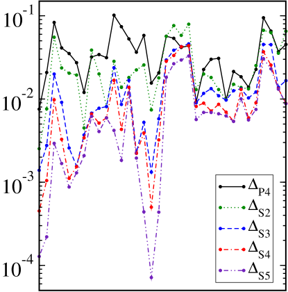
The spectral coefficients, , that determine the particular are chosen to minimize the residual for each realistic equation of state. The minimization process was carried out with an algorithm based on the Levenberg-Marquardt method Press et al. (1992), starting with initial estimates, and for . Approximate were constructed in this way for expansions containing 2, 3, 4, and 5 spectral basis functions. The minimum values of the residuals, , , , and , for these cases are listed for each equation of state in Table 1. The average values of these minimum residuals decrease from about for the 2-parameter fits, to about for the 5-parameter fits. For comparison the residuals for the 4-parameter piecewise-polytrope fits of Reid, Lackey, Owen, and Friedman Read et al. (2009) are also given in Table 1 for each equation of state.333The residuals reported in Table III of Ref. Read et al. (2009) differ from the residual listed in Table 1 in two ways. The first difference is the residuals reported in Ref. Read et al. (2009) are evaluated using base-10 logarithms, rather than the natural logarithms used here. This difference makes the Ref. Read et al. (2009) residuals smaller by the factor . The second difference is that reported here measures the accuracy of the piecewise-polytrope fits for , while the residuals reported in Ref. Read et al. (2009) measure the accuracy of those fits for where is the baryon density of the material. The values of the residuals, , , , , and , are also shown graphically in Fig. 1. Points along the horizontal axis in Fig. 1 represent the different realistic equations of state in the order listed in Table 1. These results show that the spectral fits are convergent, and do a fairly good job of approximating this collection of realistic equations of state. The 2-parameter spectral fits have smaller residuals than the 4-parameter piecewise-polytrope fits for most of these equations of state. Also listed in Table 1 are the optimal values of the spectral coefficients, , , , and , for the 4-parameter spectral approximation to each equation of state. These values, together with the tabulated constants and can be used to re-construct the complete 4-parameter spectral fits for , using Eqs. (6) and (7).
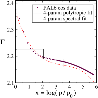
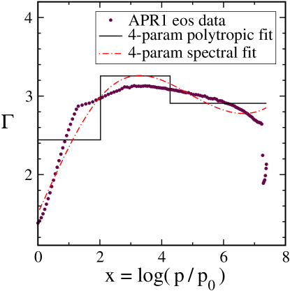
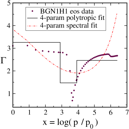
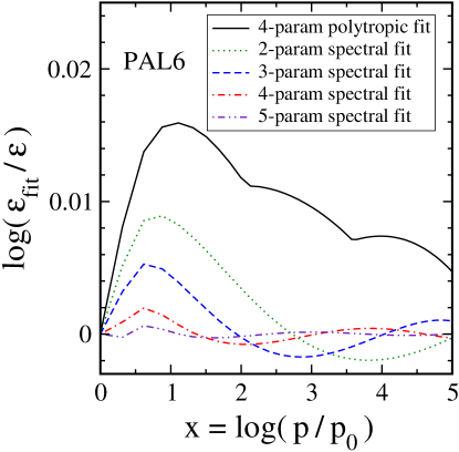
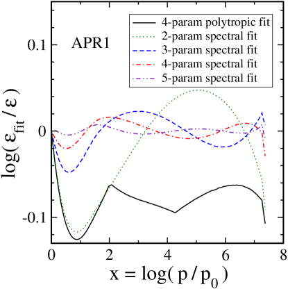
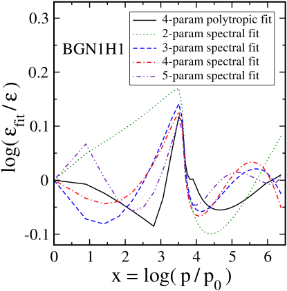
Three equations of state have been chosen from the complete set to illustrate in more detail the accuracy of the fits. These three cases are equation of state PAL6 having the highest accuracy spectral fits, APR1 having spectral fits with average accuracy, and BGN1H1 having the lowest accuracy spectral fits. Figures 2-4 show the adiabatic index computed directly from the tabulated equations of state, the 4-parameter spectral fit to the adiabatic index, and the 4-parameter piecewise-polytrope fit for each of these equations of state. From these figures it is clear that the smoother equations of state, like PAL6, have the highest accuracy fits, while the equations of state with a sharp phase transition, like BGN1H1, have the lowest accuracy fits. Figures 5-7 illustrate the errors in the various fits to the equation of state for these three example equations of state. These errors are illustrated as graphs of , as functions of the pressure variable . These figures show that the spectral fits are much more accurate than the 4-parameter piecewise-polytrope fit for the smooth and average equations of state, PAL6 and APR1. The spectral fits have about the same accuracy as the piecewise-polytrope fit for equation of state BGN1H1 which has a strong phase transition. Figures 5-7 also illustrate in a visual way the convergence of the spectral fits as the number of basis functions is increased.
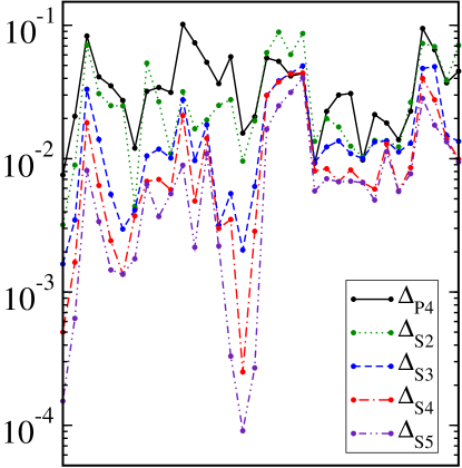
The enthalpy based representation of the equation of state, and , is more useful for certain purposes. It is helpful to understand, therefore, whether the spectral fits for this representation, Eqs. (14)–(19), are as accurate and effective as those for the standard representation. So approximate equations of state, , have been constructed for the same set of 34 realistic neutron star equations of state described in Ref. Read et al. (2009). As before these fits were made by adjusting the values of the spectral coefficients defined in Eq. (14), to minimize the residual defined in (20). The only differences between this and the standard case are: The variable is chosen here to be an enthalpy variable, and the functions and are determined here with Eqs. (17)–(19). Table 2 lists each equation of state, along with the residuals, , , , and , for the spectral fits having 2, 3, 4 and 5 non-zero spectral coefficients. The values of the residuals, , , , , and , are also show graphically in Fig. 8 for these enthalpy based fits. Table 2 also lists the coefficients, , , , and for the 4-parameter spectral fit. Finally, Table 2 contains information about the enthalpy variables, and , for each equation of state. The quantity is the enthalpy for which and whose values are listed in Table 1, and is the value for which . These results show that the spectral expansions of the enthalpy based representation of the equation of state are very comparable to the standard expansions.
| EOS | ||||||||||
|---|---|---|---|---|---|---|---|---|---|---|
| PAL6 | 0.0032 | 0.0016 | 0.0005 | 0.0002 | 0.8608 | -0.1509 | 0.0909 | -0.0192 | 0.0405 | 2.62 |
| SLy | 0.0089 | 0.0035 | 0.0017 | 0.0006 | 1.0077 | 0.2084 | -0.1266 | 0.0203 | 0.0314 | 3.22 |
| AP1 | 0.0708 | 0.0331 | 0.0186 | 0.0081 | 0.5205 | 1.3288 | -0.7804 | 0.1316 | 0.0276 | 3.31 |
| AP2 | 0.0307 | 0.0139 | 0.0063 | 0.0034 | 0.7557 | 0.6423 | -0.3586 | 0.0604 | 0.0287 | 3.34 |
| AP3 | 0.0250 | 0.0054 | 0.0024 | 0.0015 | 0.9520 | 0.4691 | -0.2109 | 0.0273 | 0.0298 | 3.40 |
| AP4 | 0.0249 | 0.0030 | 0.0014 | 0.0014 | 0.8824 | 0.4064 | -0.1405 | 0.0135 | 0.0297 | 3.41 |
| FPS | 0.0044 | 0.0041 | 0.0037 | 0.0018 | 1.1462 | -0.1088 | 0.0432 | -0.0106 | 0.0279 | 3.23 |
| WFF1 | 0.0521 | 0.0105 | 0.0068 | 0.0064 | 0.7115 | 0.8263 | -0.3258 | 0.0372 | 0.0273 | 3.53 |
| WFF2 | 0.0267 | 0.0118 | 0.0070 | 0.0037 | 0.8527 | 0.6162 | -0.3135 | 0.0512 | 0.0285 | 3.48 |
| WFF3 | 0.0109 | 0.0101 | 0.0058 | 0.0054 | 1.3660 | -0.4236 | 0.2293 | -0.0469 | 0.0253 | 3.30 |
| BBB2 | 0.0318 | 0.0277 | 0.0210 | 0.0089 | 0.8447 | 0.8101 | -0.5808 | 0.1120 | 0.0297 | 3.24 |
| BPAL12 | 0.0168 | 0.0097 | 0.0048 | 0.0022 | 1.0847 | -0.6537 | 0.4289 | -0.0874 | 0.0373 | 2.73 |
| ENG | 0.0195 | 0.0179 | 0.0142 | 0.0109 | 1.0426 | 0.4716 | -0.3353 | 0.0632 | 0.0286 | 3.39 |
| MPA1 | 0.0251 | 0.0032 | 0.0030 | 0.0022 | 1.0523 | 0.3546 | -0.1356 | 0.0074 | 0.0297 | 3.33 |
| MS1 | 0.0277 | 0.0055 | 0.0035 | 0.0003 | 0.9340 | 0.2231 | 0.0718 | -0.0642 | 0.0485 | 2.73 |
| MS2 | 0.0096 | 0.0021 | 0.0003 | 0.0001 | 0.9680 | -0.1326 | 0.0786 | -0.0360 | 0.0367 | 2.56 |
| MS1b | 0.0192 | 0.0062 | 0.0029 | 0.0003 | 1.2148 | -0.1255 | 0.1959 | -0.0700 | 0.0403 | 2.92 |
| PS | 0.0624 | 0.0298 | 0.0298 | 0.0166 | 1.3064 | -1.2479 | 0.5534 | -0.0186 | 0.0571 | 2.26 |
| GS1 | 0.0889 | 0.0383 | 0.0377 | 0.0249 | 1.7649 | -1.9609 | 0.8871 | -0.0942 | 0.0265 | 3.22 |
| GS2 | 0.0603 | 0.0437 | 0.0433 | 0.0314 | 1.2562 | -0.4936 | -0.1125 | 0.1051 | 0.0362 | 2.61 |
| BGN1H1 | 0.0868 | 0.0495 | 0.0439 | 0.0403 | 1.1915 | 0.2463 | -0.7222 | 0.2300 | 0.0356 | 2.97 |
| GNH3 | 0.0135 | 0.0093 | 0.0081 | 0.0057 | 1.0236 | 0.0297 | -0.2197 | 0.0742 | 0.0482 | 2.53 |
| H1 | 0.0200 | 0.0122 | 0.0084 | 0.0071 | 1.0365 | 0.1735 | -0.5519 | 0.1790 | 0.0406 | 2.39 |
| H2 | 0.0173 | 0.0136 | 0.0067 | 0.0067 | 1.0666 | 0.4639 | -0.8300 | 0.2393 | 0.0391 | 2.41 |
| H3 | 0.0124 | 0.0109 | 0.0082 | 0.0068 | 1.1204 | 0.2084 | -0.5285 | 0.1519 | 0.0402 | 2.42 |
| H4 | 0.0103 | 0.0100 | 0.0066 | 0.0066 | 1.0070 | 0.4040 | -0.3709 | 0.0696 | 0.0223 | 3.18 |
| H5 | 0.0137 | 0.0134 | 0.0059 | 0.0049 | 0.9614 | 0.6257 | -0.6459 | 0.1371 | 0.0233 | 2.96 |
| H6 | 0.0137 | 0.0135 | 0.0129 | 0.0113 | 1.0182 | 0.1483 | -0.2638 | 0.0628 | 0.0263 | 2.79 |
| H7 | 0.0123 | 0.0112 | 0.0057 | 0.0057 | 0.9147 | 0.4331 | -0.4779 | 0.1064 | 0.0254 | 2.94 |
| PCL2 | 0.0265 | 0.0130 | 0.0086 | 0.0077 | 1.0127 | 0.1289 | -0.4822 | 0.1616 | 0.0389 | 2.52 |
| ALF1 | 0.0731 | 0.0475 | 0.0400 | 0.0283 | 0.9349 | -0.3810 | 0.6697 | -0.2305 | 0.0305 | 2.75 |
| ALF2 | 0.0692 | 0.0490 | 0.0276 | 0.0178 | 0.7100 | 2.6577 | -2.2438 | 0.4712 | 0.0305 | 2.83 |
| ALF3 | 0.0386 | 0.0149 | 0.0140 | 0.0134 | 0.8987 | 0.4588 | -0.3533 | 0.0489 | 0.0305 | 2.73 |
| ALF4 | 0.0708 | 0.0135 | 0.0099 | 0.0094 | 0.8705 | 0.4469 | 0.0284 | -0.0914 | 0.0305 | 2.83 |
| Average | 0.0323 | 0.0166 | 0.0124 | 0.0089 |
IV Discussion
The spectral fits constructed here were designed to explore how accurately the real neutron-star equation of state might be determined once the first few accurate neutron-star mass-radius measurements become available. These fits could be improved for equations of state with phase transitions by using separate spectral fits above and below the phase-transition pressure. These piecewise spectral fits could eliminate Gibbs phenomena errors, but would require significantly more (roughly double the number of) parameters. Measuring this larger number of parameters from neutron-star observations would therefore require a much larger number of accurate mass-radius determinations. A systematic study of the relative accuracy of single versus piecewise spectral expansions (with the same total number of free parameters) will therefore be delayed until more neutron-star measurements become available.
The fits constructed here show that spectral representations of the various realistic neutron-star equations of state are remarkably accurate, even when the number of basis functions used in the spectral expansion is rather small. Such expansions provide an attractive alternative to the piecewise-polytrope approximations for a variety of current “realistic” models of the equation of state. If the real neutron-star equation of state is relatively smooth, then these spectral expansions will provide an extremely efficient way to represent it. And remarkably, even if the neutron-star equation of state has a phase transition, these spectral fits do about as well as the piecewise polytrope fits with the same number of free parameters.
Acknowledgements.
I thank Benjamin Owen, Benjamin Lackey, John Friedman, and Chris Vuille for helpful discussions about their work, B.O., B.L. and C.V. for useful comments on an earlier draft of this paper, and B.L and J.F. for providing tables of the various realistic equations of state used here. This research was supported in part by a grant from the Sherman Fairchild Foundation, by NSF grant PHY-0601459, and by NASA grant NNX09AF97G.References
-
Shapiro and Teukolsky (1983)
S. L. Shapiro and
S. A. Teukolsky,
Black Holes, White
Dwarfs and Neutron Stars (Wiley, New York, 1983). - Read et al. (2009) J. S. Read, B. D. Lackey, B. J. Owen, and J. L. Friedman, Phys. Rev. D79, 124032 (2009).
- Oppenheimer and Volkoff (1939) J. R. Oppenheimer and G. M. Volkoff, Physical Review 55, 374 (1939).
- Lindblom (1992) L. Lindblom, Astrophys. J. 398, 569 (1992).
- Arnett and Bowers (1977) W. D. Arnett and R. L. Bowers, Ap. J. Suppl. Ser. 33, 415 (1977).
- Lattimer and Prakash (2007) J. M. Lattimer and M. Prakash, Phys. Rep. 442, 109 (2007).
- Steiner et al. (2010) A. W. Steiner, J. M. Lattimer, and E. F. Brown (2010), arXiv:1005.0811.
- Prakash et al. (1988) M. Prakash, T. L. Ainsworth, and J. M. Lattimer, Phys. Rev. Lett. 61, 2518 (1988).
- Glendenning (1985) N. K. Glendenning, Astrophys. J. 293, 470 (1985).
- Vuille (1995) C. Vuille (1995), unpublished; arXiv:0812.3828.
-
Vuille and Ipser (1999)
C. Vuille and
J. Ipser, in
Eighth Canadian Conference on
General Relativity and Relativistic Astrophysics, edited by C. P. Burgess and R. C. Meyers (1999), vol. 493 of AIP Conference Proceedings, p. 60. - Haensel and Potekhin (2004) P. Haensel and A. Y. Potekhin, Astron. Astrophys. 428, 191 (2004).
- Shibata et al. (2005) M. Shibata, K. Taniguchi, and K. Uryu, Phys. Rev. D 71, 084021 (2005).
- Shibata and Taniguchi (2006) M. Shibata and K. Taniguchi, Phys. Rev. D 73, 064027 (2006).
- Zdunik et al. (2006) J. L. Zdunik, M. Bejger, P. Haensel, and E. Gourgoulhon, Astron. Astrophys. 450, 747 (2006).
- Press et al. (1992) W. H. Press, S. A. Teukolsky, W. T. Vetterling, and B. P. Flannery, Numerical Recipes in FORTRAN (Cambridge University Press, Cambridge, England, 1992), 2nd ed.