Radiation Magnetohydrodynamics for Black Hole-Torus System in Full General Relativity: A Step toward Physical Simulation

Abstract

A radiation-magnetohydrodynamic simulation for the black hole-torus system is performed in the framework of full general relativity for the first time. A truncated moment formalism is employed for a general relativistic neutrino radiation transport. Several systems in which the black hole mass is $M_{\rm BH}=3$ or $6M_{\odot}$, the black hole spin is zero, and the torus mass is $\approx 0.14$–$0.38M_{\odot}$ are evolved as models of the remnant formed after the merger of binary neutron stars or black hole-neutron star binaries. The equation of state and microphysics for the high-density and high-temperature matter are phenomenologically taken into account in a semi-quantitative manner. It is found that the temperature in the inner region of the torus reaches $\mathrel{\raise 1.29167pt\hbox{$>$}\mkern-14.0mu\lower 2.58334pt\hbox{$\sim$}}10$ MeV which enhances a high luminosity of neutrinos $\sim 10^{51}$ ergs/s for $M_{\rm BH}=6M_{\odot}$ and $\sim 10^{52}$ ergs/s for $M_{\rm BH}=3M_{\odot}$. It is shown that neutrinos are likely to be emitted primarily toward the outward direction in the vicinity of the rotational axis and their energy density may be high enough to launch a low-energy short gamma-ray burst via the neutrino-antineutrino pair-annihilation process with the total energy deposition $\sim 10^{47}$–$10^{49}$ ergs. It is also shown in our model that for $M_{\rm BH}=3M_{\odot}$, the neutrino luminosity is larger than the electromagnetic luminosity while for $M_{\rm BH}=6M_{\odot}$, the neutrino luminosity is comparable to or slightly smaller than the electromagnetic luminosity.

1 Introduction

The latest numerical simulations show that the merger of black hole-neutron star binaries and binary neutron stars often produces a system composed of a black hole surrounded by a massive torus of mass $\mathrel{\raise 1.29167pt\hbox{$>$}\mkern-14.0mu\lower 2.58334pt\hbox{$\sim$}}0.1M_{\odot}$ [1, 2, 3, 4, 5, 6]. Such systems are promising candidates for the central engine of short-hard gamma-ray bursts (SGRB) [7] which emit a huge amount of total radiation energy $\sim 10^{48}$–$10^{50}$ ergs in a short time scale $\mathrel{\raise 1.29167pt\hbox{$<$}\mkern-14.0mu\lower 2.58334pt\hbox{$\sim$}}2$ s [8]. The proposed mechanism for emitting the huge radiation energy is the pair annihilation of neutrinos and antineutrinos which are emitted from the hot and massive torus surrounding the central black hole (e.g., Ref. SJR) or electromagnetic mechanisms such as Blandford-Znajek mechanism, by which rotational energy of a black hole can be efficiently extracted [10, 11], and/or Blandford-Payne mechanism (or similar mechanisms) by which rotational energy of the torus can be extracted by the magneto-centrifugal effect [12, 13].

To clarify the hypotheses that the black hole-torus system could be the central engine of SGRB, a general-relativistic magnetohydrodynamic (GRMHD) simulation including neutrino radiation effects is probably the unique approach. If we focus on the neutrino-pair-annihilation scenario for generating the huge gamma-ray luminosity, the effect of the neutrino radiation transport has to be taken into account. In a previous paper [14], we performed a GRMHD simulation (in a fixed Kerr spacetime background) including microphysics effects as well as neutrino cooling, extending the earlier Newtonian and non-magnetohydrodynamics works (e.g., Refs. SJR,LRP). However, to date, no simulation has been done in the framework of general-relativistic, radiation-magnetohydrodynamics (GRRMHD).

In this paper, we report results of our first GRRMHD simulation for the evolution of black hole-torus systems as a step toward a more physical simulation incorporating with the detailed microphysics. The simulation is performed in full general relativity and in the framework of ideal magnetohydrodynamics (MHD): We solve Einstein’s equation, MHD equation, induction equation, and a radiation transport equation. For evolving the radiation field of neutrinos, we employ a truncated moment formalism as suggested in Refs. AS,Kip,SKSS11. For simplicity, in this work, we do not consider the distribution in the frequency space (spectrum) nor the flavor of neutrinos. We employ a phenomenological equation of state (EOS) for the high-density (with maximum density $\rho_{\rm max}=0.5$–$3.0\times 10^{12}~{}{\rm g/cm^{3}}$) torus matter and treat cross sections between matter and neutrinos in an approximate manner. We believe that even with these approximate treatments, this work qualitatively and semi-quantitatively captures a transport effect of neutrinos and coupling effects among general relativity, MHD, and neutrino radiation transport for the first time.

This paper is organized as follows. In §2, the formulation for our present GRRMHD simulation is summarized. In §3, the initial condition for the black hole-torus system is given. In §4, EOS for the matter in the torus, and coupling terms between the matter and radiation are specified. We also describe our numerical method for the evolution of the system. After a brief summary of quantities for diagnostics in §5, numerical results are shown in §6, focusing in particular on the luminosities of neutrinos and electromagnetic radiations. Section 7 is devoted to a summary. In Appendixes A and B, we present numerical results for test simulations to show that our radiation hydrodynamic code is reliable. Throughout this paper, the geometrical units of $c=1=G$ are employed unless otherwise stated, where $c$ is the speed of light and $G$ the gravitational constant. Greek ($\alpha$, $\beta$, $\gamma\cdots$) and Latin ($i$, $j$, $k\cdots$) subscripts denote the spacetime and space components, respectively. The radiation quantities will be denoted by the Calligraphy.

2 Formulation and basic equations

2.1 Framework

We solve Einstein’s equation, continuity equation for baryons, MHD equation, induction equation, and a radiation transport equation all together assuming the axial symmetry and the equatorial plane symmetry for the system for the system. The basic equations are

$$G_{\mu\nu}=8\pi(T_{\mu\nu}^{\rm MHD}+{\cal T}_{\mu\nu}^{\rm rad}),$$ (1)

$$\nabla_{\mu}(\rho u^{\mu})=0,$$ (2)

$$\nabla^{\mu}T_{\mu\nu}^{\rm MHD}=-\cal{S}^{\rm rad}_{\nu},$$ (3)

$$\nabla_{\mu}F^{*\mu\nu}=0,$$ (4)

$$\nabla^{\mu}\cal{T}_{\mu\nu}^{\rm rad}=\cal{S}^{\rm rad}_{\nu},$$ (5)

where $G_{\mu\nu}$ is Einstein’s tensor, $\rho$ is the rest-mass density of baryon, $u^{\mu}$ is the four velocity, $\nabla_{\mu}$ is the covariant derivative with respect to the spacetime metric $g_{\mu\nu}$, $T_{\mu\nu}^{\rm MHD}$ and ${\cal T}_{\mu\nu}^{\rm rad}$ are the stress-energy tensors of MHD and radiation (neutrinos) parts, ${\cal S}^{\rm rad}_{\nu}$ is the source term of the radiation field, and $F^{*\mu\nu}$ is the dual of the electromagnetic tensor, respectively. In this paper, we assume that the ideal MHD condition holds and write $F^{*\mu\nu}$ as

$$F^{*\mu\nu}=b^{\mu}u^{\nu}-b^{\nu}u^{\mu},$$ (6)

where $b^{\mu}$ denotes the magnetic field vector defined in the fluid rest frame, i.e., $b_{\mu}u^{\mu}=0$.

The stress-energy tensors are written as

$$T_{\mu\nu}^{\rm MHD}=(\rho h+b^{2})u_{\mu}u_{\nu}+\Big{(}P+{b^{2}\over 2}\Big{)}g_{\mu\nu}-b_{\mu}b_{\nu},$$ (7)

$${\cal T}_{\mu\nu}^{\rm rad}={\cal J}u_{\mu}u_{\nu}+{\cal H}_{\mu}u_{\mu}+{\cal H}_{\nu}u_{\mu}+{\cal L}_{\mu\nu},$$ (8)

where $h$ is the specific enthalpy defined by $1+\varepsilon+P/\rho$ with $\varepsilon$ and $P$ being the specific internal energy and pressure, and $b^{2}=b_{\mu}b^{\mu}$. ${\cal J}$, ${\cal H}_{\mu}$, and ${\cal L}_{\mu\nu}$ are the energy density, momentum density, and stress tensor of the radiation field , which are defined from the distribution function $f$ by [18]

$${\cal J}=h_{\rm pl}^{4}\int d\omega\omega^{3}\int f(\omega,\Omega,x^{\mu})d\Omega,$$ (9)

$${\cal H}^{\alpha}=h_{\rm pl}^{4}\int d\omega\omega^{3}\int\ell^{\alpha}f(\omega,\Omega,x^{\mu})d\Omega,$$ (10)

$${\cal L}^{\alpha\beta}=h_{\rm pl}^{4}\int d\omega\omega^{3}\int\ell^{\alpha}\ell^{\beta}f(\omega,\Omega,x^{\mu})d\Omega,$$ (11)

where $h_{\rm pl}$ is the Planck constant, $\omega$ is the frequency of the radiation, $\int d\Omega$ denotes the integration over the solid angle on unit sphere, and $\ell^{\alpha}$ is a spacelike unit normal vector orthonormal to $u^{\alpha}$; $\ell^{\mu}\ell_{\mu}=1$ and $\ell_{\mu}u^{\mu}=0$. Note that we do not consider the evolution of the spectrum for the radiation field for simplicity in this work. We also define the stress-energy tensor for the electromagnetic field by

$$T_{\mu\nu}^{\rm EM}=b^{2}u_{\mu}u_{\nu}+{b^{2}\over 2}g_{\mu\nu}-b_{\mu}b_{\nu}.$$ (12)

2.2 Einstein’s equation

Einstein’s evolution equations are solved using the original version of Baumgarte-Shapiro-Shibata-Nakamura formulation [20] together with the so-called moving-puncture variable [21]. Specifically, we evolve a conformal factor $W\equiv\gamma^{-1/6}$, the conformal three-metric $\tilde{\gamma}_{ij}\equiv\gamma^{-1/3}\gamma_{ij}$, the trace of the extrinsic curvature $K$, the conformal trace-free part of the extrinsic curvature $\tilde{A}_{ij}\equiv\gamma^{-1/3}(K_{ij}-K\gamma_{ij}/3)$, and an auxiliary variable $F_{i}\equiv\tilde{\gamma}_{ij,j}$. Here, $\gamma_{ij}$ and $K_{ij}$ are the spatial metric and the extrinsic curvature, respectively. For the evolution of the geometrical variables, we implicitly assume to use the Cartesian coordinates; the cartoon method is used for solving Einstein’s equation[22].

The spatial derivatives in the evolution equations are evaluated by a fourth-order centered finite difference except for the advection terms which is evaluated by a fourth-order up-wind finite difference. A fourth-order Runge-Kutta method is employed for the time integration. We employ a moving-puncture gauge for the lapse function $\alpha$ and shift vector $\beta^{k}$ (e.g., Ref. BB4) in the form

$$\partial_{t}\alpha = -2\alpha K,$$ (13)

$$\partial_{t}\beta^{i} = {3\over 4}\tilde{\gamma}^{ij}(F_{j}+\Delta t\partial_{t}F_{j}),$$ (14)

where $\Delta t$ is the time step. We omit the advection terms in Eqs. (13) and (14) because black holes are located at the origin in the present setting and thus the advection terms do not play an important role.

2.3 MHD equations

MHD equations are solved in the same numerical scheme as shown in Ref. SS05 to which the reader may refer. Specifically, we choose the following variables to be evolved,

$$S_{0}=W^{-3}T_{\mu\nu}^{\rm MHD}n^{\mu}n^{\nu},$$ (15)

$$S_{i}=-W^{-3}T_{\mu\nu}^{\rm MHD}n^{\mu}\gamma^{\nu}_{~{}i},$$ (16)

where $n^{\alpha}$ is the unit normal to spacelike hypersurfaces for which the components are

$$n^{\alpha}=\Big{(}{1\over\alpha},-{\beta^{k}\over\alpha}\Big{)}.$$ (17)

The Euler and energy equations are written in the forms

$$\partial_{t}S_{i}+{1\over\sqrt{\eta}}\partial_{j}(\sqrt{\eta}S_{ik}\gamma^{jk})=-S_{0}\partial_{i}\alpha+S_{j}\partial_{i}\beta^{j}-{1\over 2}\alpha S_{jk}\partial_{i}\gamma^{jk}-\alpha W^{-3}{\cal S}^{\rm rad}_{i},$$ (18)

$$\partial_{t}S_{0}+{1\over\sqrt{\eta}}\partial_{j}(\sqrt{\eta}\alpha S^{j})=\alpha K^{ij}S_{ij}-S^{i}\partial_{i}\alpha+\alpha W^{-3}{\cal S}^{\rm rad}_{\alpha}n^{\alpha},$$ (19)

where $S_{ij}=W^{-3}T^{\rm MHD}_{\alpha\beta}\gamma^{\alpha}_{~{}i}\gamma^{\beta}_{~{}j}$, $S^{i}=\gamma^{ij}S_{j}$, and $\eta$ is the determinant of the flat metric in the curvilinear coordinates.

The induction equation is solved defining a magnetic-field variable

$$B^{\mu}=W^{-3}(wb^{\mu}-\alpha b^{t}u^{\mu}),$$ (20)

where $w=\alpha u^{t}$ and $B^{\mu}n_{\mu}=0$. We only need to solve the spatial component $B^{i}$ by

$$\partial_{t}B^{i}={1\over\sqrt{\eta}}\partial_{j}[\sqrt{\eta}(B^{j}v^{i}-B^{j}v^{i})],$$ (21)

where $v^{i}=u^{i}/u^{t}$ is the three velocity.

The transport terms are specifically evaluated using a Kurganov-Tadmor scheme [28] with a piecewise parabolic reconstruction for the quantities of cell interfaces. The fourth-order Runge-Kutta method is employed for the time integration. For solving the induction equation, a constrained-transport scheme with second-order interpolation in space is employed [26].

2.4 Radiation

In the numerical simulation, instead of using Eq. (8), we rewrite ${\cal T}_{\alpha\beta}^{\rm rad}$ as [18]

$${\cal T}_{\alpha\beta}^{\rm rad}={\cal E}_{0}n_{\alpha}n_{\beta}+({\cal F}_{0})_{\alpha}n_{\beta}+({\cal F}_{0})_{\beta}n_{\alpha}+({\cal P}_{0})_{\alpha\beta},$$ (22)

and solve the equations for ${\cal E}_{0}$ and $({\cal F}_{0})_{k}$. Here, $({\cal P}_{0})^{\alpha\beta}n_{\alpha}=0=({\cal F}_{0})^{\alpha}n_{\alpha}$. ${\cal J}$ and ${\cal H}_{\alpha}$ are determined by

$${\cal J}={\cal E}_{0}w^{2}-2({\cal F}_{0})^{k}wu_{k}+({\cal P}_{0})^{ij}u_{i}u_{j},$$ (23)

$${\cal H}^{\alpha}=({\cal E}_{0}w-({\cal F}_{0})^{k}u_{k})h^{\alpha}_{~{}\beta}n^{\beta}+wh^{\alpha}_{~{}\beta}({\cal F}_{0})^{\beta}-h^{\alpha}_{~{}i}u_{j}({\cal P}_{0})^{ij},$$ (24)

where $h_{\alpha\beta}=g_{\alpha\beta}+u_{\alpha}u_{\beta}$. We here note $h^{\alpha}_{~{}\beta}n^{\beta}=n^{\alpha}-wu^{\alpha}$ and $n_{\alpha}h^{\alpha\beta}\gamma_{\beta k}=-wu_{k}$. The introduction of ${\cal E}_{0}$ and $({\cal F}_{0})_{i}$ allows us to write the basic equations in a conservative form as

$$\partial_{t}{\cal E}+{1\over\sqrt{\eta}}\partial_{j}[\sqrt{\eta}(\alpha{\cal F}^{j}-\beta^{j}{\cal E})]$$

$$\hskip 56.9055pt=\alpha[{\cal P}^{ij}K_{ij}-{\cal F}^{j}\partial_{j}\ln\alpha-W^{-3}{\cal S}^{\rm rad}_{\alpha}n^{\alpha}],$$ (25)

$$\partial_{t}{\cal F}_{i}+{1\over\sqrt{\eta}}\partial_{j}[\sqrt{\eta}(\alpha{\cal P}_{i}^{~{}j}-\beta^{j}{\cal F}_{i})]$$

$$\hskip 56.9055pt=\Big{[}-{\cal E}\partial_{i}\alpha+{\cal F}_{k}\partial_{i}\beta^{k}-{\alpha\over 2}{\cal P}_{jk}\partial_{i}\gamma^{jk}+\alpha W^{-3}{\cal S}^{\rm rad}_{i}\Big{]},$$ (26)

where ${\cal E}=W^{-3}{\cal E}_{0}$, ${\cal F}_{i}=W^{-3}({\cal F}_{0})_{i}$, and ${\cal P}_{ij}=W^{-3}({\cal P}_{0})_{ij}$. Hence, the equations can be integrated in the same numerical scheme (high-resolution shock capturing scheme) as the MHD equations.

In the truncated moment formalism employed here, we have to impose a closure relation for determining ${\cal P}_{ij}$. We follow Ref. SKSS11 on the prescription for this (we employ the simplest version of Ref. SKSS11.) For the optically thin limit, we set

$$({\cal P}^{ij})_{\rm thin}={\cal E}{{\cal F}^{i}{\cal F}^{j}\over\gamma_{kl}{\cal F}^{k}{\cal F}^{l}},$$ (27)

and for the optically thick limit,

$${\cal L}^{\alpha\beta}={1\over 3}h^{\alpha\beta}{\cal J}.$$ (28)

Equation (28) is rewritten in terms of ${\cal P}^{ij}$, ${\cal E}$, and ${\cal F}_{i}$ as

$$({\cal P}^{ij})_{\rm thick} = {{\cal E}\over 2w^{2}+1}\Big{[}(2w^{2}-1)\gamma^{ij}-4V^{i}V^{j}\Big{]}+{1\over w}({\cal F}^{i}V^{j}+{\cal F}^{j}V^{i})$$ (29)

$$~{}+{2{\cal F}^{k}u_{k}\over(2w^{2}+1)w}(-w^{2}\gamma^{ij}+V^{i}V^{j}),$$

where $V^{k}=\gamma^{kl}u_{l}$.

For the optically grey region, we assume

$${\cal P}^{ij}={3\chi-1\over 2}({\cal P}^{ij})_{\rm thin}+{3(1-\chi)\over 2}({\cal P}^{ij})_{\rm thick},$$ (30)

where $\chi$ is the so-called variable Eddington factor, which is $\chi=1/3$ in the optically thick limit and $\chi=1$ in the optically thin limit. Following Ref. Livermore, we write $\chi$ as a function of $\hat{\cal F}$, for which we choose [18]

$${\hat{\cal F}}:=\biggl{(}{h_{\alpha\beta}{\cal H}^{\alpha}{\cal H}^{\beta}\over{\cal J}^{2}}\biggr{)}^{1/2}.$$ (31)

Following Livermore [24], we employ the following function for $\chi({\hat{\cal F}})$ as

$$\chi={3+4{\hat{\cal F}}^{2}\over 5+2\sqrt{4-3{\hat{\cal F}}^{2}}}.$$ (32)

With the choice of (31), $\hat{F}$ obeys an algebraic equation for a given set of ${\cal E}$ and ${\cal F}_{j}$. This can be written in the form

$$\hat{\cal F}^{2}={h^{\alpha\gamma}{\cal T}_{\alpha\beta}^{\rm rad}u^{\beta}{\cal T}_{\gamma\lambda}^{\rm rad}u^{\lambda}\over{\cal T}_{\alpha\beta}^{\rm rad}u^{\alpha}u^{\beta}},$$ (33)

where for ${\cal T}_{~{}\alpha\beta}^{\rm rad}$, Eq. (22) is used with Eq. (30). In the numerical simulation, we solve this algebraic equation numerically.

3 Initial condition

In this work, we perform simulations for the system composed of a stellar-mass black hole surrounded by a high-density torus. Such a system is a possible outcome after the merger of binary neutron stars and black hole-neutron star binaries. The latest simulations have indeed shown that a massive disk may be formed after the merger (see, e.g., Refs. REV for a review): For a total mass of the system 3–$8M_{\odot}$, the disk mass could be 0.1–$0.5M_{\odot}$ with the maximum density $10^{11}$–$10^{13}~{}{\rm g/cm^{3}}$ (for binary parameters and EOS which are favorable for a disk formation). Generally speaking, the disk formation is enhanced if (i) the black hole in the black hole-neutron star binary is rapidly spinning [6] or (ii) the EOS of neutron stars is stiff (the radius of neutron stars is large) enough for the merger to result in a long-lived hypermassive neutron star for the binary neutron stars [4, 5].

In this work, we set the black hole mass to be $M_{\rm BH}=3M_{\odot}$ or $6M_{\odot}$, and baryon rest-mass of the disk to be $M_{\rm disk}\approx 0.14$–$0.38M_{\odot}$. The system with $M_{\rm BH}=3M_{\odot}$ is a model for the remnant of the binary neutron star merger and that with $M_{\rm BH}=6M_{\odot}$ is a model for black hole-neutron star binaries. The nondimensional black hole spin is chosen to be $a=0$ for simplicity: In a previous paper [14], we show that the prograde spin enhances the neutrino luminosity, and hence, the results of the present paper are likely to give a conservative estimate for the neutrino luminosity. The maximum density $\rho_{\rm max}$ is chosen in the range $2.3$–$3.1\times 10^{12}~{}{\rm g/cm^{3}}$ for $M_{\rm BH}=3M_{\odot}$ and $5.1$–$7.5\times 10^{11}~{}{\rm g/cm^{3}}$ for $M_{\rm BH}=6M_{\odot}$. We note that for the same mass and radius of the disk in units of $M_{\rm BH}$, the density is lower for the higher-mass black hole. For these initial conditions, we prepare an equilibrium state which is constructed by a code reported in Ref. S07 with the so-called $j$-constant law in which all the fluid elements have the same specific angular momentum (the same value of $hu_{\varphi}$). Table 1 lists key quantities for the initial conditions.

Table 1: Key quantities for the initial conditions employed in the numerical simulation. Black hole mass ($M_{\rm BH}$), nondimensional spin parameter ($a$), location (in terms of the coordinate radius) of the inner and outer edges on the equatorial plane, baryon rest mass and maximum density of the torus, maximum magnetic field strength, and maximum ratio of the magnetic pressure to the gas pressure. $M_{\rm BH}$ and $M_{\rm disk}$ are shown in units of $M_{\odot}$. $r_{1}$ and $r_{2}$ are shown in units of $M_{\rm BH}(GM_{\rm BH}/c^{2})$.

Model	$M_{\rm BH}$	$a$	$(r_{1},r_{2})$	$M_{\rm disk}$	$\rho_{\rm max}[{\rm g/cm^{3}}]$	$B_{\rm max}$ (G)	$(P_{B}/P_{\rm gas})_{\rm max}$
6a0m4	6	$0.0$	$(6.00,17.65)$	$0.242$	$5.12\times 10^{11}$	$3.4\times 10^{14}$	1.6%
6a0m6	6	$0.0$	$(6.00,18.05)$	$0.381$	$7.45\times 10^{11}$	$3.6\times 10^{14}$	1.5%
3a0m1	3	$0.0$	$(4.00,18.05)$	$0.145$	$2.28\times 10^{12}$	$1.1\times 10^{15}$	2.3%
3a0m2	3	$0.0$	$(4.00,18.53)$	$0.209$	$3.08\times 10^{12}$	$1.0\times 10^{15}$	1.6%

At $t=0$, we superimpose a poloidal magnetic field inside the torus which induces an angular momentum transport during the evolution as in, e.g., Refs. MG,SST07. Such an initial magnetic field configuration is chosen simply due to the technical reason: In the nearly vacuum region, we cannot put magnetic fields for which the magnetic pressure is much larger than the (atmosphere) gas pressure because our MHD code is not allowed to evolve an extremely low-$\beta$ plasma. Note that even if the magnetic field profile is initially artificial, the resulting profile after several dynamical timescale evolution depends only weakly on the initial condition, as described in many papers in this field (e.g., Ref MG): The resulting magnetic fields are usually composed of a random magnetic field inside the torus and of approximately dipole magnetic fields outside the torus and black hole magnetosphere. These seem to be a universal outcome after the onset of magnetohydrodynamical instabilities. Thus we adopt a simple magnetic field profile initially.

The profile for the toroidal component of the vector potential of the magnetic field is chosen as

$$A_{\varphi}=\left\{\begin{array}[]{ll}A_{0}(P-P_{0})&{\rm for}~{}P>P_{0},\\ 0&{\rm for}~{}P\leq P_{0},\end{array}\right.$$ (36)

and then the magnetic field is given by

$$B^{i}=W^{-3}\epsilon^{ijk}\partial_{j}A_{k},$$ (37)

where $\epsilon^{ijk}$ is the completely antisymmetric tensor. $P_{0}$ is a parameter chosen to be $0.04P_{\rm max}$ where $P_{\rm max}$ is the maximum pressure. $A_{0}$ is the constant that determines the magnetic field strength. In this paper, we give a strong magnetic field initially to make the angular momentum transport turn on immediately after the onset of simulations. The given maximum magnetic field strength is $B_{\rm max}\approx 3$–$5\times 10^{14}$ G for $M_{\rm BH}=6M_{\odot}$ and $\approx 1\times 10^{15}$ G for $M_{\rm BH}=3M_{\odot}$, with which the maximum ratio of the magnetic pressure to the gas pressure is $\sim 1.5$–2.3% (see Table 1). A latest GRMHD simulation for the binary neutron star merger indicates that such a strong magnetic field will be achieved during the evolution of accretion torus surrounding central black holes [3].

We employed the different field strength for a few models as a test and found that the results depend very weakly on it as far as the field strength is sufficiently large. For a weak initial field strength, by contrast, the angular momentum transport does not proceed efficiently, and hence, the degree of the subsequent turbulent motion is weak and the efficiency of the shock heating is also low. The likely reason is that with the weak field strength, the fastest growing mode of the magnetorotational instability (MRI) is not resolved. The strong magnetic field has to be set up to enhance the efficient angular momentum transport and shock heating in the present grid resolution.

4 Equation of state and treatment of radiation

4.1 Equation of state

For a high-density matter with $\rho\sim 10^{10}$–$10^{13}~{}{\rm g/cm^{3}}$, the dominant pressure sources are degenerate electrons and thermal nucleons for the typical temperature $10^{10}$–$10^{11}$ K. The pressure for them is written, respectively, by

$$P_{\rm deg}=4.93\times 10^{30}\Big{(}{Y_{e}\rho_{12}\over 0.5}\Big{)}^{4/3}~{}{\rm g/cm/s^{2}},$$ (38)

$$P_{\rm gas}=8.31\times 10^{29}\rho_{12}T_{10}~{}{\rm g/cm/s^{2}},$$ (39)

where $\rho_{12}=\rho/(10^{12}~{}{\rm g/cm^{3}})$, $Y_{e}$ is the fraction of electrons per nucleon, and $T_{10}=T/(10^{10}$ K). We here assume that the baryon is composed only of free nucleons. The radiation pressure due to photons and electron-positron pairs is written as

$$P_{\gamma}=\Big{(}{1\over 3}+{7\over 12}\Big{)}a_{\rm r}T^{4}=7.04\times 10^{25}T_{10}^{4}~{}{\rm g/cm/s^{2}},$$ (40)

where $a_{\rm r}$ is the radiation density constant ($7.56\times 10^{-15}~{}{\rm ergs/cm^{3}/K^{4}}$). The effect of the radiation pressure on dynamics is minor in the main body of the torus where $\rho_{12}\mathrel{\raise 1.29167pt\hbox{$>$}\mkern-14.0mu\lower 2.58334pt\hbox{$\sim$}}1$, as far as $T_{10}\mathrel{\raise 1.29167pt\hbox{$<$}\mkern-14.0mu\lower 2.58334pt\hbox{$\sim$}}10$, although the radiation pressure plays a role for a high-temperature and relatively low-density region that does not contribute much to the neutrino luminosity. Hence, we ignore its contribution to the pressure.

Thus, for simplicity, we employ the following EOS:

$$P=K\rho^{4/3}+(\Gamma_{\rm th}-1)\rho\varepsilon_{\rm th},$$ (41)

where $K$ is a polytropic constant which is $4.93\times 10^{14}(Y_{e}/0.5)^{4/3}$ (in the cgs unit) for degenerate relativistic electrons [30], and $\Gamma_{\rm th}$ is the adiabatic constant for which we choose $5/3$, because free nucleons mainly contribute to the thermal part. $\varepsilon_{\rm th}$ is the specific thermal energy determined by

$$\varepsilon_{\rm th}=\varepsilon-\varepsilon_{\rm poly},$$ (42)

where $\varepsilon_{\rm poly}=3K\rho^{1/3}$ is the specific internal energy associated with degenerate electrons. In this paper, we give a fixed value for $Y_{e}$ as 0.3; we suppose a moderately neutron-rich material.

The matter temperature may be determined from the relation

$$k_{\rm B}T={2\over 3}m_{u}\varepsilon_{\rm th},$$ (43)

where $m_{u}$ is the atomic mass unit ($m_{u}=1.66057\times 10^{-24}$ g), and $k_{\rm B}$ is the Boltzmann constant. Specifically,

$$T=7.206\times 10^{10}\Big{(}{\varepsilon_{\rm th}\over 0.01c^{2}}\Big{)}~{}{\rm K}.$$ (44)

In reality, the temperature does not increase linearly with $\varepsilon_{\rm th}$, because the contribution of the radiation (photons and electron-positron pairs) to the internal energy in fact becomes significant for high temperature; see Eq. (40). Instead of solving the 4th order nonlinear equation for $T$, we simply set a maximum value for the temperature to be $k_{\rm B}T_{\rm max}=30$ MeV: A latest fully general relativistic simulation shows that this is indeed a reasonable upper bound [5]. If the value of $T$, determined from Eq. (44), exceeds $T_{\rm max}$, we set $T=T_{\rm max}$. This procedure may give a higher estimation of $T$ for $10\mathrel{\raise 1.29167pt\hbox{$<$}\mkern-14.0mu\lower 2.58334pt\hbox{$\sim$}}T_{10}\mathrel{\raise 1.29167pt\hbox{$<$}\mkern-14.0mu\lower 2.58334pt\hbox{$\sim$}}30$. However, the density of such high temperature region is rather small as $\rho\mathrel{\raise 1.29167pt\hbox{$<$}\mkern-14.0mu\lower 2.58334pt\hbox{$\sim$}}10^{8-9}$ g/cm³ (see the top and middle panels of Fig. 1), and hence, spurious effects of this simple procedure seem to be minor.

4.2 Radiation source term

The source term for the radiation transport equation, $S^{\rm rad}_{\alpha}$, is determined in the following manner. For neutrinos in the medium with $\rho\sim 10^{11}$–$10^{13}~{}{\rm g/cm^{3}}$, the dominant process is the absorption by nucleons [31, 32, 33]. Taking into account this fact, we write it as

$${\cal S}^{\rm rad}_{\alpha}=\kappa[({\cal J}^{\rm eq}(T)-{\cal J})u_{\alpha}-{\cal H}_{\alpha}],$$ (45)

where we write for simplicity,

$${\cal J}^{\rm eq}={7\over 8}a_{\rm r}T^{4},$$ (46)

assuming that neutrinos are close to the $\beta$-equilibrium. This assumption is reasonable in the main part of the torus. Note that $T$ in Eq. (46) is the matter temperature. We here assume that only electron neutrinos and anti-neutrinos are present. Because we omit other sources for the neutrino emission such as pair production process and also emission of muon and tau neutrinos, the total neutrino luminosity is likely to be underestimated. However, the present treatment is acceptable for a qualitative and semi-quantitative study, e.g., to derive an approximate order of magnitude of the neutrino luminosity. $\kappa$ is the opacity and we here define by $\rho\sigma c/m_{u}$ where $\sigma$ is the cross section of neutrinos with matter. For simplicity, we write it

$$\sigma=C_{\sigma}\sigma_{\rm w}\Big{(}{k_{\rm B}T\over m_{e}c^{2}}\Big{)}^{2},$$ (47)

where $\sigma_{\rm w}=1.76\times 10^{-44}~{}{\rm cm^{2}}$ denotes the characteristic cross section of weak interactions [30], $m_{e}c^{2}$ is the electron rest-mass energy, 511 KeV, and $C_{\sigma}$ is a constant which we choose 1; we choose $C_{\sigma}=0.5$ and 2 for test simulations, but the results (evolution of torus and neutrino luminosity) depend only weakly on this parameter. The dependence on the neutrino energy is simply estimated by the local matter temperature $k_{\rm B}T$, because we do not have the method for estimating it in the present treatment. In the optically thick region, our prescription is acceptable. However, in the grey and optically thin regions, a more sophisticated treatment is required.

For this choice of $\sigma$, a nondimensional quantity $\kappa GM_{\rm BH}/c^{3}$ is written as

$${\kappa GM_{\rm BH}\over c^{3}}=3.6C_{\sigma}\rho_{12}\Big{(}{k_{\rm B}T\over 10~{}{\rm MeV}}\Big{)}^{2}\Big{(}{M_{\rm BH}\over 6M_{\odot}}\Big{)}.$$ (48)

Thus, a torus of thickness $\sim 10GM_{\rm BH}/c^{2}$ and of temperature $k_{\rm B}T=10$ MeV surrounding a black hole of mass $6M_{\odot}$ is optically thick for $\rho\mathrel{\raise 1.29167pt\hbox{$>$}\mkern-14.0mu\lower 2.58334pt\hbox{$\sim$}}3\times 10^{10}~{}{\rm g/cm^{3}}$ with $C_{\sigma}=1$.

4.3 Partial implicit scheme

The timescale of the neutrino absorption and emission $\approx\kappa^{-1}$ is often shorter than the dynamical timescale of the system $\sim GM_{\rm BH}/c^{3}\sim 0.03$ ms. This prohibits the explicit time integration of the radiation transport equations. For a stable numerical computation, we employ a partial implicit (explicit-implicit) scheme for the time integration. Schematically, Eqs. (25) and (26) are written in a matrix form

$$\partial_{t}\mbox{\boldmath$F$}=\mbox{\boldmath$T$}+\kappa(\mbox{\boldmath$S$}_{0}-\mbox{\boldmath$A$}\mbox{\boldmath$F$}),$$ (49)

where $F$ denotes a vector composed of

$$\mbox{\boldmath$F$}=\left(\begin{array}[]{l}{\cal E}\\ {\cal F}_{x}\\ {\cal F}_{y}\\ {\cal F}_{z}\\ \end{array}\right).$$ (54)

$T$ denotes the sum of the transport term $\partial_{i}(\cdots)^{i}$ and the source term associated with the gravitational fields. $\mbox{\boldmath$S$}_{0}$ denotes the source term composed of the thermal quantity $a_{\rm r}T^{4}$, and $A$ is a $4\times 4$ matrix composed of the hydrodynamic and geometric quantities. In each Runge-Kutta time integration, the term $\partial_{t}\mbox{\boldmath$F$}$ is discretized as $(\mbox{\boldmath$F$}^{n+1}-\mbox{\boldmath$F$}^{n})/\Delta t$ where $n$ and $n+1$ denote neighboring two time steps for the fourth-order Runge-Kutta time integration ($n=0$–3). In the partial implicit scheme employed here, $n$-th quantities are assigned for $T$, $\mbox{\boldmath$S$}_{0}$, $A$, and $\kappa$, while we assign ($n+1$)-th quantities for $F$ in the right-hand side. Namely, we write the equation in the following form:

$$(1+\kappa^{n}\Delta t\mbox{\boldmath$A$}^{n})\mbox{\boldmath$F$}^{n+1}=\mbox{\boldmath$F$}^{n}+\Delta t(\mbox{\boldmath$T$}^{n}+\kappa^{n}\mbox{\boldmath$S$}_{0}^{n}).$$ (55)

This is a simple $4\times 4$ matrix equation and solved in a straightforward manner.

After the radiation transport equations are integrated, we integrate the MHD equations. The transport term and ordinary source term associated with the gravitational field of this equation are handled in the same manner as in our previous paper; to obtain the ($n+1$)-th quantities, $n$-th quantities are assigned for these terms. In the right-hand side of the MHD equations, the source terms composed of the radiation fields are included additionally in the present case; $-\kappa(\mbox{\boldmath$S$}_{0}-\mbox{\boldmath$A$}\mbox{\boldmath$F$})$. We handle this term as in the radiation transport equation, i.e., in the following time stepping:

$$-\kappa^{n}(\mbox{\boldmath$S$}_{0}^{n}-\mbox{\boldmath$A$}^{n}\mbox{\boldmath$F$}^{n+1}).$$ (56)

This implies that the absolute value of the source term associated with the radiation field in the MHD equations is equal to that in the radiation transport equation, and hence, the energy and momentum contributed from this source term cancel each other for the total conservation equation $\nabla^{\mu}(T_{\mu\nu}^{\rm MHD}+{\cal T}_{\mu\nu}^{\rm rad})=0$.

In Appendix A, we present results of a test simulation using a semi-analytic solution of radiation-hydrodynamical Bondi flow. In Appendix B, we also present results of one-dimensional test simulations of Riemann problems in special relativity. We show that by our code, it is feasible to stably perform a radiation hydrodynamics simulation and also to derive a second-order convergent result for high values of $\kappa$ (for the optically thick case) for the general relativistic flows.

5 Quantities for diagnostics

We monitor the total baryon rest-mass $M_{*}$, internal energy $E_{\rm int}$, thermal component of internal energy $E_{\rm th}$, kinetic energy $T_{\rm kin}$, and electromagnetic energy $E_{\rm B}$ by

$$M_{*}=\int\rho_{*}\sqrt{\eta}d^{3}x,$$ (57)

$$E_{\rm int}=\int\rho_{*}\varepsilon\sqrt{\eta}d^{3}x,$$ (58)

$$E_{\rm th}=\int\rho_{*}\varepsilon_{\rm th}\sqrt{\eta}d^{3}x,$$ (59)

$$T_{\rm kin}=\int{1\over 2}\rho_{*}hv^{i}u_{i}\sqrt{\eta}d^{3}x,$$ (60)

$$E_{\rm B}=\int T^{\rm EM}_{\mu\nu}n^{\mu}n^{\nu}\alpha^{-1}\sqrt{\eta}d^{3}x.$$ (61)

Here, for the definition of $E_{\rm int}$, $T_{\rm kin}$, and $E_{\rm B}$, we follow Ref. DLSSS2. Note that $M_{*}=M_{\rm disk}$ at initial.

In stationary axisymmetric spacetimes, the following relations are derived from the conservation law of the energy-momentum tensor in the absence of neutrino cooling:

$$\partial_{\mu}(\sqrt{-g}(T^{{\rm MHD}})^{\mu}_{~{}t})=0.$$ (62)

From this relation, it is natural to define the ejection rate of energy

$$\dot{E}=-\oint_{r={\rm const}}(T^{{\rm MHD}})^{r}_{~{}t}\sqrt{-g}dS,$$ (63)

where $dS=d\theta d\varphi$ and the surface integral is performed for a two surface far from the torus. From the continuity equation, the rest-mass ejection rate is defined in the same manner as

$$\dot{M}_{*}=\oint_{r={\rm const}}\rho_{*}v^{r}r^{2}dS.$$ (64)

Emission rates of energy for the electromagnetic field and radiation are defined in the same manner as

$$\dot{E}_{\rm B}=-\oint_{r={\rm const}}(T^{{\rm EM}})^{r}_{~{}t}\sqrt{-g}dS,$$ (65)

$$\dot{E}_{\rm rad}=-\oint_{r={\rm const}}({\cal T}^{{\rm rad}})^{r}_{~{}t}\sqrt{-g}dS.$$ (66)

Pair annihilation rates of neutrinos and antineutrinos are roughly evaluated in the following manner: First we assume that the luminosity of neutrinos and antineutrinos are $c_{\nu}e$ and $(1-c_{\nu})e$, respectively. Here, $c_{\nu}$ is a constant for which $0<c_{\nu}<1$. Then the pair annihilation luminosity per volume is approximately estimated by [35]

$$\dot{q}_{\nu\bar{\nu}}=c_{\rm max}c\sigma_{0}{e^{2}\over(m_{e}c^{2})^{2}}\sqrt{E_{\nu}E_{\bar{\nu}}},$$ (67)

where $c_{\rm max}={\rm max}[c_{\nu}^{2},(1-c_{\nu})^{2}]\cos^{2}\Theta$ with $\Theta$ being the collision angle of pairs. Note that the maximum value of $c_{\rm max}$ is $1/4$. The typical value of $\Theta$ is determined by the configuration of the neutrino-emission region: If the pair annihilation occurs in the vicinity of the black hole and rotation axis, $\cos\Theta$ is likely to be near the unity. $\sigma_{0}(\approx 3.3\times 10^{-45}~{}{\rm cm}^{2})$ is the typical cross section of the pair annihilation, and $E_{\nu}$ and $E_{\bar{\nu}}$ are the characteristic energy of neutrinos and antineutrinos, respectively. From $\dot{q}_{\nu\bar{\nu}}$, we define an approximate pair annihilation luminosity by

$$L_{\nu\bar{\nu}}=\int W^{-3}dV\dot{q}_{\nu\bar{\nu}}.$$ (68)

In the following, we show the result of $L_{\nu\bar{\nu}}$ with $c_{\rm max}\sqrt{E_{\nu}E_{\bar{\nu}}}/(m_{e}c^{2})=1/4$ as a reference for the order of magnitude of $L_{\nu\bar{\nu}}$.

6 Numerical results

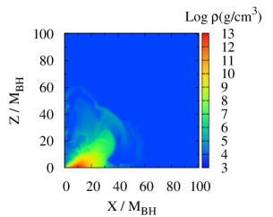
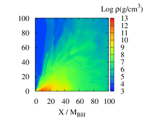
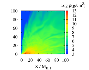
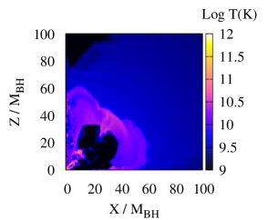
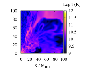
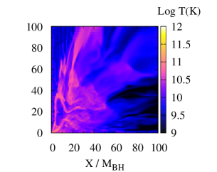
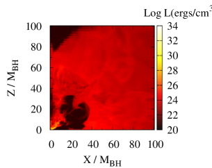
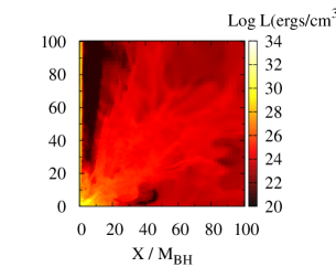
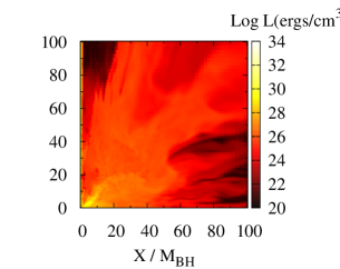
Figure 1: Snapshots for the distribution of the rest-mass density (top panels), matter temperature (middle panels), and radiation field density (${\cal E}_{0}={\cal E}W^{3}$, bottom panels) at selected time slices, $t=5.7$ ms (left), 21.3 ms (middle), and 42.5 ms (right), for model 3a0m2.

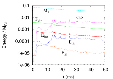
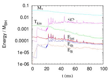
Figure 2: Evolution of the total rest-mass energy ($M_{*}$), kinetic energy ($T_{\rm kin}$), internal energy ($E_{\rm int}$), thermal energy ($E_{\rm th}$), and electromagnetic energy ($E_{\rm B}$) measured outside the apparent horizon for models 3a0m2 (left) and 6a0m4 (right) as in Fig. 1. We also plot an averaged value of the specific internal energy defined by $\langle\varepsilon\rangle=E_{\rm int}/M_{*}$.

6.1 Setting

Numerical simulations are performed in a nonuniform grid with the $(x,z)$ coordinates. In addition, we prepare 5 grid points along the $y$ direction for solving Einstein’s equation by the Cartoon method [22] with the fourth-order accuracy. The grid spacing for each coordinate at $i$-th grid point is determined by the following rule,

$$\Delta x_{i}=\left\{\begin{array}[]{ll}\Delta x_{0}&{\rm for}~{}0\leq x\leq x_{\rm in},\\ C_{x}\Delta x_{i-1}&{\rm for}~{}x\geq x_{\rm in},\\ \end{array}\right.$$ (71)

where $\Delta x_{0}$ is a constant, $\Delta x_{i}=x_{i+1}-x_{i}$, and $x_{i}$ is the $i$-th grid point with $0\leq i\leq N$. Here, $x_{i}$ denotes $x$ or $z$. For $y$, the grid is set at $\pm\Delta x_{0}$ and $\pm 2\Delta x_{0}$. $C_{x}$ is a constant which is set to be 1.016. We employ $(N,\Delta x_{0})=(630,0.05M_{\rm BH})$ and $(500,0.075M_{\rm BH})$ for the high and low grid resolutions, respectively. $x_{\rm in}=20M_{\rm BH}$ and $22.5M_{\rm BH}$ for $N=630$ and 500. With this setting, the outer boundary along each axis for the high- and low-resolution runs is located at $x_{N}=139M_{\rm BH}$ and $132M_{\rm BH}$, respectively. By several test simulations, we confirmed that the numerical results depend only weakly on the grid resolution. Hence, we only show the results for the higher-resolution runs in the following.

6.2 General features of dynamics

In the axisymmetric simulation, the magnetic field eventually escapes from the torus after the amplification of the magnetic-field strength saturates. The reason is that the dynamo action is not sustained in the axisymmetric system because of the anti dynamo property [36]. Thus, an extremely long-term simulation does not provide a realistic result because the angular momentum transport process induced by the MHD effect does not work in its late phase. Keeping in mind this fact, we always stopped the simulations at $t=3500M_{\rm BH}$ following Ref. MG. This corresponds to $\approx 50$ ms and 100 ms for $M_{\rm BH}=3M_{\odot}$ and $6M_{\odot}$, respectively.

Figure 1 plots the snapshots for the distribution of the rest-mass density, matter temperature, and radiation field density (${\cal E}_{0}={\cal E}W^{3}$) at $t=5.7$, 21.3, and 42.5 ms for model 3a0m2. This shows the universal qualitative features for the evolution of the system: After the simulation is started, the magnetic-field strength increases due to the winding and MRI caused by the differential rotation (see Fig. 2). These processes also play an active role for transporting angular momentum from inner parts to outer parts of the torus. Due to the increase of the magnetic-field pressure, the matter is ejected from the torus predominantly toward the high latitude (see the left panels of Fig. 1). By this process, the geometrical thickness of the matter distribution increases, resulting in formation of a quasisteady funnel structure which is composed of the geometrically thick torus and a nearly vacuum region in the vicinity of the rotational axis (see the middle and right panels of Fig. 1). Due to the angular momentum transport process, on the other hand, the matter for which angular momentum is removed falls into the BH, and the total mass of the torus gradually decreases. A part of the matter ejected from the torus to a high latitude comes back to the torus. If the angular momentum of the matter is extracted by the magnetic processes during its travel, the matter eventually comes back to an inner region of the torus. When it hits the torus, a shock is generated and its kinetic energy is liberated. As a consequence of this process which continuously occurs, the temperature of the inner region of the torus increases to a value larger than 10 MeV, and such a region becomes a primary emission region of neutrinos.

Because a funnel structure is formed and the neutrino emission is most active near the inner region of the torus, neutrinos are emitted primarily toward the outward direction in the vicinity of the rotational axis. The bottom panels of Fig. 1 indeed shows that the neutrino radiation density is high in a cone around the rotational axis and the opening angle of the cone is rather small (cf. Fig. 3). Due to this collimation property, the radiation density is enhanced. This is a favorable property for an efficient pair annihilation of neutrinos and antineutrinos near the rotational axis.

6.3 Energetics

6.3.1 General feature

Figure 2 plots the evolution of the total rest-mass energy ($M_{*}$), kinetic energy ($T_{\rm kin}$), internal energy ($E_{\rm int}$), thermal energy ($E_{\rm th}$), and electromagnetic energy ($E_{\rm B}$), for which the integrations (57)–(61) are performed for the region outside the apparent horizon, as well as an averaged value of the specific internal energy defined by $E_{\rm int}/M_{*}$ for models 3a0m2 (left) and 6a0m4 (right). The left panel of Fig. 2 quantitatively captures the features for the evolution of the system described in Fig. 1: In the first $\sim 3$ ms, the electromagnetic energy increases due to the magnetic winding and MRI. The electromagnetic energy increases to $\sim 10\%$ of the internal energy and $\sim 1\%$ of the kinetic energy. Eventually, the increase of the electromagnetic energy saturates, and then, the outflow of the material from the accretion torus and the accretion of the material into the black hole are activated. Associated with these dynamical processes, the shock heating is enhanced and the thermal energy steeply increases at $t\sim 3$ ms. The averaged value of the specific internal energy increases to $\langle\varepsilon\rangle\sim 0.003$–0.004, implying that the averaged matter temperature is $\sim 2$–3 MeV. For $t\mathrel{\raise 1.29167pt\hbox{$>$}\mkern-14.0mu\lower 2.58334pt\hbox{$\sim$}}10$ ms, the system relaxes to a quasisteady accretion phase, during which the rest mass of the torus gradually decreases. Associated with this decrease, $T_{\rm kin}$, $E_{\rm int}$, and $E_{\rm B}$ also decrease gradually. On the other hand, $\langle\varepsilon\rangle$ is approximately constant. All these quantitative features approximately hold for any model considered in this paper. This fact is observed by the comparison between the left and right panels of Fig. 2.

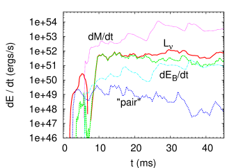
(a)   (b)

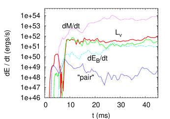
(c)   (d)

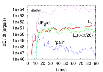
Figure 3: Matter energy ejection rate ($dM/dt$), electromagnetic luminosity ($dE_{\rm B}/dt$), neutrino luminosity ($L_{\nu}$), and an approximate estimate for the pair annihilation luminosity (“pair”) (a) for model 3a0m2, (b) for model 6a0m4, (c) for model 3a0m1, and (d) for model 6a0m6. The neutrino luminosity measured for the opening angle around the rotational axis of $\theta\leq\pi/20$ is also plotted (the curves plotted in the vicinity of $L_{\nu}$).

6.3.2 Dependence on BH mass

Figure 3 plots the evolution of the matter ejection rate ($dM/dt$), electromagnetic luminosity ($dE_{\rm B}/dt$), neutrino luminosity ($L_{\nu}$), and an approximate estimate for the pair annihilation luminosity by Eq. (67) for models (a) 3a0m2 (b) 6a0m4, (c) 3a0m1, and (d) 6a0m6. Because of the MHD activity induced by the magnetic winding and MRI, the material in the torus is ejected outward. The typical mass ejection rate is $\sim 0.1M_{\odot}$/s for $M_{\rm BH}=3M_{\odot}$ and $\sim 0.3M_{\odot}$/s for $M_{\rm BH}=6M_{\odot}$ in our employed models. After the activity of the torus turns on, the neutrino and electromagnetic luminosities are also enhanced, and these luminosities eventually relax to quasisteady values after the torus relaxes to a quasisteady state.

The typical neutrino luminosity is $\sim 10^{52}$ ergs/s for $M_{\rm BH}=3M_{\odot}$ and $\sim 10^{51}$ ergs/s for $M_{\rm BH}=6M_{\odot}$ in our models. Thus, it is higher for the lower black hole mass. By contrast, the dependence of the electromagnetic luminosity, $\sim 10^{51}$ ergs/s, on the black hole mass is not as strong as that of the neutrino luminosity. The electromagnetic luminosity has a positive correlation with $dM/dt$ as $dE_{\rm B}/dt=C_{\rm EM}dM/dt$. The weak dependence of the ratio coefficient $C_{\rm EM}\sim 3\times 10^{-2}$ indicates that the mass ejection is driven by the electromagnetic power. An important point indicated in this work is that for the lower-mass black-hole system, the neutrino emission is the primary dissipation mechanism, while for the higher-mass case, the electromagnetic wave emission plays the primary role. We do not fully take into account the relevant microphysical processes and the results presented in this paper are approximate ones. However, it is strongly likely that a critical mass, which divides the dominant dissipation mechanism, exists. The reason for this mass dependence will be explained as follows.

The weak dependence of $dE_{\rm B}/dt$ on the black hole mass may be explained assuming that it is proportional to $B^{2}R^{3}\Omega$ as in the Blandford-Payne mechanism [12, 13]. Here, $B$, $R$, and $\Omega$ are the typical magnetic-field strength, radius, and angular velocity of the torus. We note that for the models employed in this paper, the black hole spin is zero (or small, as a result of accretion), and hence, the Blandford-Znajek mechanism is not relevant [10]. The present models also have the parameters $R/M_{\rm BH}\sim 10$ and $\Omega\propto M_{\rm BH}^{-1}$ universally. For the saturated magnetic field strength, $B^{2}$ is approximately proportional to the gas pressure $P\propto\rho c_{s}^{2}\sim\rho T$ where $c_{s}$ is the sound velocity. Here, $T$ depends only weakly on the black hole mass, and we have an approximate relation $\rho\propto M_{\rm BH}^{-2}$ for a given mass and radius of the torus. Thus, $B^{2}$ should be proportional to $M_{\rm BH}^{-2}T$, and $B^{2}R^{3}\Omega\propto M_{\rm BH}^{0}T$: $dE_{\rm B}/dt$ should depend only weakly on the black hole mass. This agrees with the present numerical results.

The dependence of the neutrino luminosity on the black hole mass may be estimated in the following manner. Suppose that the mass accretion rate of a torus into the black hole is $\dot{M}_{\rm in}$. Then, the accretion luminosity $L_{\rm acc}$ is approximately written as $M_{\rm BH}\dot{M}_{\rm in}/R$. Because $M_{\rm BH}/R$ is $\sim 0.1$ depending weakly on the black hole mass, $L_{\rm acc}\propto\dot{M}_{\rm in}$. For a given disk mass, $\dot{M}_{\rm in}\sim M_{\rm disk}/\tau$ where $\tau$ is the accretion time scale which should be proportional to $M_{\rm BH}$. Thus, $L_{\rm acc}\propto M_{\rm BH}^{-1}$. If the neutrino luminosity is proportional to $L_{\rm acc}$, it should be proportional to $M_{\rm BH}^{-1}$: For the smaller black hole mass, the neutrino luminosity should be larger. This agrees qualitatively with the present numerical results.

6.3.3 Neutrino pair annihilation luminosity

In Fig. 3, the neutrino luminosity measured for the angle $\theta\leq\pi/20$ is also plotted. Comparing this with the total neutrino luminosity shows that neutrinos are emitted substantially toward the outward direction along the rotation axis. This is likely to come from the facts that the inner region of the torus has the maximum temperature and that a funnel structure is formed after the magnetic instabilities turn on. This collimation effect enhances the neutrino radiation density near the axis, and as a result, the efficiency of the pair annihilation of neutrinos and antineutrinos will be also enhanced.

The pair annihilation luminosity depends most strongly on the black hole mass. The reason is that it is proportional to the square of the neutrino luminosity. For the binary-neutron-star model with $M_{\rm BH}=3M_{\odot}$, the typical magnitude is $10^{48}$–$10^{49}$ ergs/s whereas for the black-hole-neutron-star-binary model with $M_{\rm BH}=6M_{\odot}$, it is $\sim 10^{47}$ ergs/s. For a hypothetical duration of the neutrino emission $\sim 100$ ms for $M_{\rm BH}=3M_{\odot}$, the total energy deposited could be $\sim 10^{48}$ ergs. This value could explain the total energy of relatively weak SGRB. By contrast, for $M_{\rm BH}=6M_{\odot}$, the total energy could be at most $10^{47}$ ergs even for the time duration of 1 s. This is too low to explain the observed SGRB. However, a word of the note is appropriate here. First, we do not take into account some of important neutrino emission processes and realistic microphysics in this work. The neutrino luminosity could be higher than that estimated in this work in reality. If so, the pair-annihilation luminosity could be higher than that presented in this paper. Second, we do not consider the spin of black holes, although a black hole of a relatively high spin is likely to be formed for the merger of binary neutron stars and black hole-neutron star binaries. For such a high-spin black hole, the neutrino luminosity could be by one order of magnitude larger than that presented in this paper [37, 14]. This suggests that the pair-annihilation luminosity could be by two order of magnitude larger for the case that a black hole has a high spin. More detailed study taking into account the detailed microphysics and high black hole spin is the issue for our subsequent work.

7 Summary

We present our first numerical result of the GRRMHD simulation for black hole-torus systems in the framework of full general relativity. Taking into account the latest results of the numerical-relativity simulation for black hole-neutron star binaries and binary neutron stars, we evolve the systems of $M_{\rm BH}=3M_{\odot}$ or $6M_{\odot}$ and of the torus mass $0.14$–$0.38M_{\odot}$ with the maximum density of the torus $5\times 10^{11}$–$3\times 10^{12}~{}{\rm g/cm^{3}}$. We incorporate some of neutrino processes (absorption and emission via the interaction with free nucleons) in an approximate manner. The following is the summary for the results obtained in this paper:

• The typical order of the neutrino luminosity is $10^{52}$ ergs/s for $M_{\rm BH}=3M_{\odot}$ and $10^{51}$ ergs/s for $M_{\rm BH}=6M_{\odot}$. Because we do not take into account some of important processes of the neutrino emission, these values may be considered as a lower bound for the neutrino luminosity.

• Neutrinos are dominantly emitted toward the outward direction along the rotation axis of the accretion torus. The reason is that after MHD instabilities set in, a high-temperature region appears in the inner edge of the accretion torus and also a funnel structure, which enhances the emission toward the direction along the rotational axis, is formed.

• The order of the electromagnetic luminosity is $10^{51}$ ergs/s and it depends only weakly on the black hole mass in our present models. Thus, for $M_{\rm BH}=3M_{\odot}$, the neutrino luminosity is larger than the electromagnetic luminosity, while for $M_{\rm BH}=6M_{\odot}$, two luminosities are comparable. The order-of-magnitude estimate supports this result, and hence, it is likely that there is a critical black hole mass above which the neutrino luminosity is smaller than the electromagnetic luminosity.

• A very approximate estimate for the total pair annihilation rate of neutrino-antineutrino pairs suggests that the order of the magnitude of the luminosity associated with this process is $10^{49}$ ergs/s for $M_{\odot}=3M_{\odot}$ and $10^{47}$ ergs/s for $M_{\odot}=6M_{\odot}$. Again, these values may be considered as a lower bound because we do not incorporate some of important processes of the neutrino emission nor the black hole spin; the value may be underestimated by a factor of 10–100. Taking into account this fact, the present results suggest that SGRB with relatively low energy may be driven from the remnants formed from the merger of black hole-neutron star binaries and binary neutron stars, respectively.

Acknowledgments

This work was supported by Grant-in-Aid for Scientific Research (21018008, 21105511, 21340051, 23740160), by Grant-in-Aid for Scientific Research on Innovative Area (20105004), and by HPCI Strategic Program of Japanese MEXT.

Appendix A Radiation field in the optically thick spherical flow

As shown in Refs. AS,SKSS11, it is possible to derive an approximate solution of the radiation field in the optically thick limit using the diffusion approximation. We here describe the analytic solution of the Bondi flow in the framework of radiation hydrodynamics, i.e., an accretion flow of the matter and radiation in the Schwarzschild background [30]. We also show that our numerical code can generate the analytic solutions for the radiation flows $({\cal J},{\cal H}_{\alpha})$ and $({\cal E},{\cal F}_{i})$.

We choose the line element in the Kerr-Schild coordinates,

$$ds^{2}=-\Big{(}1-{2M\over r}\Big{)}d{\bar{t}}^{2}+{4M\over r}d{\bar{t}}dr+\Big{(}1+{2M\over r}\Big{)}dr^{2}+r^{2}(d\theta^{2}+\sin^{2}\theta d\varphi^{2}),$$ (72)

where $M$ and $r$ are the gravitational mass and areal coordinate. In this metric, the coordinate singularity at $r=2M$ does not give any messy problem.

First, we consider the optically thick limit. In this case, the total stress-energy tensor is written as

$$T^{\rm tot}_{\mu\nu}=\Big{(}\rho h+{4\over 3}{\cal J}^{\rm eq}\Big{)}u_{\mu}u_{\nu}+\Big{(}P+{1\over 3}{\cal J}^{\rm eq}\Big{)}g_{\mu\nu}.$$ (73)

Here we do not consider the magnetic field for simplicity. However, it is straightforward to take into account a purely radial magnetic field [11] and our code was already shown to reproduce such a solution [25].

In the following, we assume that the radiation is composed of photons, writing ${\cal J}^{\rm eq}=a_{\rm r}T^{4}$, and consider the case that the EOS of the matter is described by $P=K\rho^{4/3}=\rho\varepsilon/3$, i.e., the $\Gamma=4/3$ ideal fluid. Then for the ideal gas, $\varepsilon=3k_{\rm B}T/m$ where $m$ is the mass of the gas particle. In this EOS, ${\cal J}^{\rm eq}$ is written as $3K^{\prime}\rho^{4/3}$ where $K^{\prime}=a_{\rm r}(mK/k_{\rm B})^{4}/3$. Then, the total stress-energy tensor is written by

$$T^{\rm tot}_{\mu\nu}=\Big{(}\rho+4(K+K^{\prime})\rho^{4/3}\Big{)}u_{\mu}u_{\nu}+(K+K^{\prime})\rho^{4/3}g_{\mu\nu}.$$ (74)

Namely, the stress-energy tensor is the same as that for the effective EOS, $P_{\rm eff}=(K+K^{\prime})\rho^{4/3}$. This implies that it is easy to generate a Bondi solution, i.e., $\rho$, $u^{r}$, and $P_{\rm eff}$ as functions of $r$ for a given value of $K+K^{\prime}$. If the ratio of $K^{\prime}/K$ is determined, we also obtain $P$ and ${\cal J}^{\rm eq}$ as functions of $r$.

In the optically thick medium, the correction of the radiation fields in our notation is written as [18]

$${\cal J}={\cal J}^{\rm eq}+l{\cal J}^{(1)}~{}~{}{\rm and}~{}~{}{\cal H}_{i}=lH^{(1)}_{i},$$ (75)

where $l$ is the mean free path of the radiation, $\kappa^{-1}$, which is smaller than the typical size of the system (i.e., $l\ll M$), and

$${\cal J}^{(1)}=-u^{\mu}\nabla_{\mu}{\cal J}^{\rm eq}-{4\over 3}{\cal J}^{\rm eq}\nabla_{\mu}u^{\mu},$$ (76)

$${\cal H}^{(1)}_{\alpha}=-{1\over 3}h_{\alpha}^{~{}\beta}\nabla_{\beta}{\cal J}^{\rm eq}-{4\over 3}{\cal J}^{\rm eq}u^{\beta}\nabla_{\beta}u_{\alpha}.$$ (77)

Here, ${\cal J}^{\rm eq}$ is written as $3K^{\prime}P/K$. Using this relation, we find

$${\cal J}^{(1)}=0,~{}~{}~{}{\cal H}^{(1)}_{r}=-{1+u_{r}u^{r}\over 3}{\cal J}^{\rm eq}_{,r}-{4\over 3}{\cal J}^{\rm eq}\Big{(}u^{r}u_{r,r}+{M\over r^{2}}(u^{t}+u^{r})^{2}\Big{)},$$ (78)

and hence,

$${\cal J}={\cal J}^{\rm eq}+O(l^{2}),$$ (79)

$${\cal H}_{i}=l{\cal H}^{(1)}_{r}\gamma^{r}_{~{}i}+O(l^{2}).$$ (80)

In the numerical simulation, we evolve the variables ${\cal E}_{0}$ and $({\cal F}_{0})_{i}$. Then, we derive ${\cal J}$ and ${\cal H}_{i}$ using the relation for the optically thick case as

$${\cal J}={3\over 2w^{2}+1}\Big{[}(2w^{2}-1){\cal E}_{0}-2w({\cal F}_{0})_{i}V^{i}\Big{]},$$ (81)

$${\cal H}_{i}=w^{-1}({\cal F}_{0})_{i}+{1\over w(2w^{2}+1)}\Big{[}-4w^{3}{\cal E}_{0}+(4w^{2}+1)u_{i}({\cal F}_{0})_{j}V^{j}\Big{]}.$$ (82)

The test simulations were performed for a Bondi flow solution with a critical radius $12M$ and $dM/dt=1$. We set $\kappa$ to be constant and choose $\kappa=1$, 10, 30, and 100. The computational domain with $[0:50M]$ for both $x$ and $z$ is covered by the uniform grid with the grid number $N=250$, 500, and 1000. The simulations were always performed for the time duration of $50M$ because for such a duration, a relaxed converged solution is obtained. The results shown in the following are the snapshots at $t=50M$. The time step of the simulation was fixed to be $0.5\Delta x$ where $\Delta x=50M/N$.

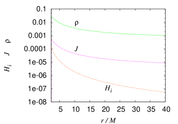
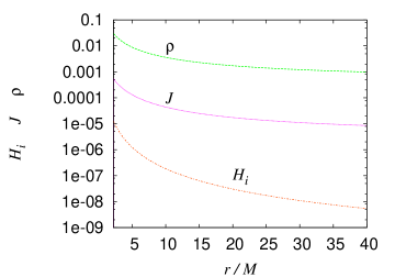
Figure 4: $\rho$, ${\cal J}$, and ${\cal H}_{i}$ as functions of $r/M$ for $\kappa=1$ (left) and 10 (right) and for $N=1000$. The points and dashed curves denote the numerical results and analytic solutions.

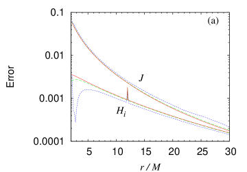
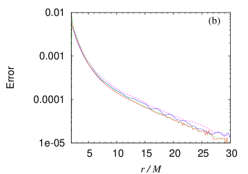
Figure 5: (a)The relative error of ${\cal J}$ and ${\cal H}_{i}$ as functions of $r/M$ for $\kappa=10$. The solid, dashed, and dotted curves are the results for $N=1000$, 500, and 250, respectively. (b) Comparison of $5[{\cal J}(N=500)-{\cal J}(N=1000)]$ (dashed curves) and $[{\cal J}(N=250)-{\cal J}(N=1000)]$ (solid curves) for $\kappa=1$ (upper) and 10 (lower curves).

Figure 4 plots $\rho$, ${\cal J}$, and ${\cal H}_{i}$ as functions of $r/M$ for $\kappa=1$ and 10, and $N=1000$. The points and solid curves are the numerical results and approximate analytic solutions valid up to $O(l)$. The data are extracted along the $x$-axis. This figure shows that the numerical computation reproduces the analytic solutions quite accurately for $\kappa=10$. For $\kappa=1$, the diffusion approximation does not accurately hold near the black hole horizon, and $H_{i}$ for the numerical solution does not agree with the analytic solution. However, for the outer region, the diffusion approximation still works. It should be noted that the magnitude of ${\cal H}_{i}$ is proportional to $\kappa^{-1}$ for $\kappa>1$. This is also found from this figure.

Next, we focus on the convergence of the numerical solutions. Figure 5(a) plots the relative errors for ${\cal J}$ and ${\cal H}_{i}$ along the $x$-axis. Here, the relative error of a quantity ${\cal Q}$ is defined by

$${\rm Error}=\Big{|}{{\cal Q}_{\rm numerical~{}solution}\over{\cal Q}_{\rm analytic~{}solution}}-1\Big{|},$$ (83)

and the analytic solution is that denoted by Eqs. (79) and (80). Figure 5(a) shows that the error does not decrease with improving the grid resolution. The reason is that the accuracy of the analytic solutions is not good enough due to the neglection of the term of order $O(l^{2})$.

To confirm that the numerical solution shows the convergent behavior, we then compare

$$5[{\cal Q}(N=500)-{\cal Q}(N=1000)]~{}~{}{\rm and}~{}~{}{\cal Q}(N=250)-{\cal Q}(N=1000),$$ (84)

where ${\cal Q}(N)$ denotes a numerical result with the grid number $N$. If the computation is second-order convergent, i.e., ${\cal Q}$ behaves as ${\cal Q}={\cal Q}(N\rightarrow\infty)+\Delta x^{2}{\cal Q}_{2}$, these two quantities should agree. Figure 5(b) compares these two quantities for ${\cal J}$ and ${\cal H}_{i}$. This indeed shows the agreement and that the numerical results are second-order convergent. Note that the reason of the violation of the second-order convergence for the error smaller than $\sim 10^{-4}$ is that other error sources come into the play for such a small error size.

Because the numerical results obey the second-order convergent behavior, it is possible to derive an exact solution for $N\rightarrow\infty$ approximately. Such an “exact” solution is different from the approximate analytic solution in which the term of $O(l)$ is not taken into account. Thus the relative difference between the “exact” solution and the analytic solution should be proportional to $\kappa^{-1}$. To confirm that the numerical solution reproduces this fact, we plot the following relative error of ${\cal H}_{r}$ in Fig. 6 for $\kappa=1$, 10, 30, and 100:

$$\Big{|}{{\cal Q}_{\rm``exact^{\prime\prime}~{}solution}\over{\cal Q}_{\rm analytic~{}solution}}-1\Big{|}.$$ (85)

It is found that this error is approximately proportional to $\kappa^{-1}$. This fact further validates our numerical solutions.

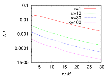
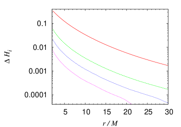
Figure 6: The relative error between the extrapolated results and analytic results of ${\cal J}$ and ${\cal H}_{i}$ as functions of $r/M$. The magnitude of the error should be proportional to $\kappa^{-1}$ and the figure shows that this is indeed the case.

Appendix B One dimensional special relativistic tests

The University of Illinois at Urbana-Champaign (UIUC) group proposed four one-dimensional test problems of the radiation hydrodynamics in special relativity [38], for the optically thick limit (the Eddington closure, ${\cal L}_{\mu\nu}={\cal J}h_{\mu\nu}/3$, is assumed). They derived four semi-analytic stationary solutions for Riemann problems. Then, they performed the following test: The derived semi-analytic solutions are boosted by a Lorentz transformation and they confirmed that their code can reproduce the boosted non-stationary solutions. However, by this test, one can check only the fact that the code can reproduce a coordinate translation of given stationary solutions.

Subsequently, Zanotti et al. [39]) proposed a more nontrivial shock tube test in which the stationary solutions by the UIUC group should be produced in a dynamical simulation: They initially prepared a discontinuous initial condition and performed simulations until the numerical data relaxes to a solution derived in Ref. UIUC. Hence, we performed the test simulations in the same manner as in Ref. Zanotti. We confirmed that our code can accurately produce these solutions as illustrated in the following.

In the test of Ref. Zanotti, the stationary solution is numerically derived preparing the initial conditions shown in Table 2. In these conditions, the discontinuity at $x=0$ is present, but during the dynamical evolution, the matter and radiation fields relax to a stationary solution after a sufficiently time duration. We performed the simulations until the stationarity was reached; the time duration of the numerical simulations is 5000 for the tests 1 and 2, 100 for the test 3, and 300 for the test 4. The numerical simulations were performed with the $\Gamma$-law EOS, $P=(\Gamma-1)\rho\varepsilon$. The opacity is assumed to have the form $\kappa=\kappa_{0}\rho$ where $\kappa_{0}$ is a given constant. The mean free path defined by $1/\kappa$ is rather long $\mathrel{\raise 1.29167pt\hbox{$>$}\mkern-14.0mu\lower 2.58334pt\hbox{$\sim$}}0.1$ in these tests, although the Eddington closure is assumed. The temperature is simply determined by $P/\rho$ during the simulation.

In the tests 1 and 2, the radiation pressure is much smaller than the gas pressure. Thus, these are the tests in which one checks whether the radiation fields are accurately evolved in an approximately fixed dynamical fluid flow with shocks. In the tests 3 and 4, the radiation pressure is as strong as or stronger than the gas pressure. These are regarded as the tests by which one checks whether the code can accurately derive the system in which both the gas and radiation play an important role.

The simulations were performed with the grid spacing $\Delta x=0.03$ for the computational domain $[-15:15]$ for the tests 1–3. For the test 4, we set $\Delta x=0.02$ with the computational domain $[-20:20]$. At the outer boundaries, we imposed the boundary condition that the fluid and radiation states remain to be the initial states which are identical with the semi-analytic solutions. The time step is set to be $0.5\Delta x$ for all the tests.

Figure 7 plots the numerical results for all the four test simulations. The solid curves and open circles denote the semi-analytic solutions and numerical results, which overlap with each other and cannot be distinguished in these figures. Thus, Fig. 7 shows that for all the four test simulations, the numerical computation satisfactorily reproduces the semi-analytic solutions, as in Refs. Zanotti. This shows an evidence that our numerical code is reliable.

Before closing this section, we note the following fact for the test 3. In this test, the stationary solution for the region $-10\mathrel{\raise 1.29167pt\hbox{$<$}\mkern-14.0mu\lower 2.58334pt\hbox{$\sim$}}x\mathrel{\raise 1.29167pt\hbox{$<$}\mkern-14.0mu\lower 2.58334pt\hbox{$\sim$}}0$ satisfies ${\cal J}^{2}<{\cal H}_{\mu}{\cal H}^{\mu}$ and ${\cal J}\ll a_{\rm r}T^{4}$. This implies that the solution is not physical, and moreover, the local thermodynamical equilibrium is not satisfied although the relation ${\cal L}_{\mu\nu}={\cal J}h_{\mu\nu}/3$ is chosen for the closure. This test is nothing but a numerical game. Thus, even if a numerical code can produce the stationary solution in this test, it might not prove that the code is suitable for physical simulations.

Table 2: The chosen constants and initial data for the one-dimensional test simulations. Adiabatic index, $\Gamma$, an artificially chosen value of $a_{\rm r}$, the value of $\kappa_{0}$, $(\rho,P,u^{x},{\cal J})$ for $x<0$ and $x>0$, respectively. $a_{\rm r}$ is determined by ${\cal J}/(P/\rho)^{4}$ for $x>0$, and then, ${\cal J}$ for $x>0$ is determined by $a_{\rm r}(P/\rho)^{4}$.

No	$\Gamma$	$a_{\rm r}$	$\kappa_{0}$	$(\rho,P,u^{x},{\cal J})_{x<0}$	$(\rho,P,u^{x},{\cal J})_{x>0}$
1	$5/3$	$10^{10}/0.81$	$0.4$	(1.0, 3.0e-5, 0.015, 1.0e-8)	(2.401, 1.612e-4, 0.006247, 2.509e-7)
2	$5/3$	$78125$	$0.2$	(1.0, 4.0e-3, 0.25, 2.0e-5)	(3.109, 0.04512, 0.0804, 3.464e-3)
3	$2$	$10^{7}/6.48$	$0.3$	(1.0, 60, 10.0, 2.0)	(7.9963, 1.25058, 2.342e3, 1.136e3)
4	$5/3$	$10^{9}/7.2$	$0.08$	(1.0, 6.0e-3, 0.69, 0.18)	(3.65, 0.3588, 1.89, 1.297)

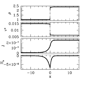
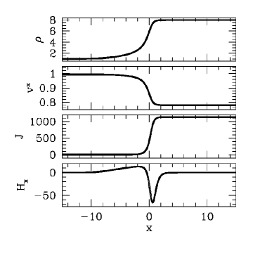
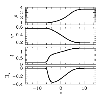
Figure 7: Numerical results for one-dimensional test problems in special relativity (test 1: top left, test 2: top right, test 3: bottom left, and test 4: bottom right). The solid curves and open circles denote the semi-analytic solutions and numerical results, respectively.

References

- [1] Z.B. Etienne, Y.-T. Liu, S.L. Shapiro, and T.W. Baumgarte, Phys. Rev. D 79 (2009), 044024; K. Kyutoku, M. Shibata, and K. Taniguchi, Phys. Rev. D 82 (2010), 044049; S. Chawla, et al., Phys. Rev. Lett. 105 (2010), 111101; F. Foucart, M.D. Duez, L.E. Kidder, and S.A. Teukolsky, Phys. Rev. D 83 (2010), 024005; K. Kyutoku, M. Shibata, and K. Taniguchi, Phys. Rev. D 84 (2011).
- [2] L. Rezzolla, et al., Class Quantum Grav. 27 (2010), 114105.
- [3] L. Rezzolla et al., Astrophys. J. Lett. 732 (2011), L6.
- [4] K. Hotokezaka, K. Kyutoku, H. Okawa, M. Shibata, and K. Kiuchi, Phys. Rev. D (2011).
- [5] Y. Sekiguchi, K. Kiuchi, K. Kyutoku, and M. Shibata, Phys. Rev. Lett. 107 (2011), 051102; Phys. Rev. Lett. 107 (2011), 211101.
- [6] M.D. Duez, Class. Quantum Grav. 27 (2010), 114002; M. Shibata and K. Taniguchi, Living Review Relativity 14 (2011), 6.
- [7] R. Narayan, B. Paczynski, and T. Piran, Astrophys. J. Lett. 395 (1992), L83.
- [8] B. Zhang and P. Mészáros, Int. J. Mod. Phys. A 19 (2004), 2385; T. Piran, Rev. Mod. Phys. 76 (2005), 1143: E. Nakar, Phys. Rev. 442 (2007), 166.
- [9] S. Setiawan, M. Ruffert, and H.-Th. Janka, Mon. Not. R. Astron. Soc. 352 (2004), 753; Astron. Astrophys. 458 (2006), 553.
- [10] R. D. Blandford and R. L. Znajek, Mon. Not. R. astr. Soc. 179 (1977), 433.
- [11] J. C. McKinney and C. F. Gammie, Astrophys. J. 611 (2004), 977; J. C. McKinney, Astrophys. J. 630 (2005), L5.
- [12] R. D. Blandford and D. G. Payne, Mon. Not. R. Astro. Soc. 199 (1982), 883.
- [13] D. Meier, Astrophys. J. 522 (1999), 753.
- [14] M. Shibata, Y. Sekiguchi, and R. Takahashi, Prog. Theor. Phys. 118 (2007), 257.
- [15] W.H. Lee, E. Ramirez-Luis, and D. Page, Astrophys. J. 632 (2005), 421.
- [16] J. L. Anderson and E. A. Spiegel, Astrophys. J. 171 (1972), 127.
- [17] K. S. Thorne, Mon. Not. R. Astro. Soc. 194 (1981), 439.
- [18] M. Shibata, K. Kiuchi, Y. Sekiguchi, and Y. Suwa, Prog. Theor. Phys. 125 (2011), 1255.
- [19] E.g., D. Mihalas and B. Weibel-Mihalas, Foundations of Radiation Hydrodynamics (Dover Publications, Inc., 1999).
- [20] M. Shibata and T. Nakamura, Phys. Rev. D 52 (1995), 5428; T. W. Baumgarte and S. L. Shapiro, Phys. Rev. D 59 (1998), 024007.
- [21] M. Campanelli, C. O. Lousto, P. Marronetti, and Y. Zlochower, Phys. Rev. Lett. 96 (2006), 111101; J. Baker et al., Phys. Rev. Lett. 96 (2006), 111102.
- [22] M. Alcubierre, S. Brandt, B. Brügmann, D. Holz, E. Seidel, R. Takahashi, and J. Thornburg, Int. J. Mod. Phys. D 10 (2001), 273; M. Shibata, Prog. Theor. Phys. 104 (2000), 325; M. Shibata, Phys. Rev. D 67 (2003), 024033.
- [23] B. Brügmann, J. A. Gonzalez, M. Hannam, S. Husa, U. Sperhake, and W. Tichy, Phys. Rev. D 77 (2008), 024027.
- [24] C. D. Livermore, J. Quant. Spectrosc. Radiat. Transfer 31 (1984), 149.
- [25] M. Shibata and Y. Sekiguchi, Phys. Rev. D 72 (2005), 044014.
- [26] C. R. Evans and J. F. Hawley, Astrophys. J. 332 (1988), 659.
- [27] Y. Sekiguchi, Prog. Theor. Phys. 124 (2010), 331.
- [28] A. Kurganov and E. Tadmor, J. Comp. Phys. 160 (2000), 241.
- [29] M. Shibata, Phys. Rev. D 76 (2007), 064035.
- [30] S.L. Shapiro and S.A. Teukolsky, Black holes, White dwarfs, and Neutron stars: the Physics of Compact Objects (Wiley, 1983), chapter 14.
- [31] D. L. Tubbs abd D. N. Schramm, Astrophys. J. 201 (1975), 467.
- [32] S. W. Bruenn, Astrophys. J. Supplement 58 (1985), 771.
- [33] M. Rampp, Radiation Hydrodynamics with Neutrinos: Stellar Core Collapse and the Explosion Mechanism of Type II Supernovae, Ph.D Thesis, Max-Planck-Institut fur Astrophysik, 2002.
- [34] M. D. Duez, Y. T. Liu, S. L. Shapiro, M. Shibata, and B. C. Stephens, Phys. Rev. D 73 (2006), 104015.
- [35] A. M. Belborodov, AIP Conf. Proc. 1054 (2008), 51.
- [36] H. K. Moffatt, Magnetic Field Generation in Electrically Conducting Fluids (Cambridge Univ. Press, 1978).
- [37] W.-X. Chen and A. M. Belborodov, Astrophys. J 657 (2007), 383.
- [38] B.D. Farris, T.K. Li, Y.T. Liu, and S.L. Shapiro, Phys. Rev. D 78 (2008), 024023.
- [39] O. Zanotti, C. Roedig, L. Rezzolla, and L. Del Zanna, Mon. Not. R. Astron. Soc. 416 (2011).