Changes to neoclassical flow and bootstrap current in a tokamak pedestal

Abstract

In a tokamak pedestal, radial scale lengths can become comparable to the ion orbit width, invalidating conventional neoclassical calculations of flow and bootstrap current. In this work we illustrate a non-local approach that allows strong radial density variation while maintaining small departures from a Maxwellian distribution. Non-local effects alter the magnitude and poloidal variation of the flow and current. The approach is implemented in a new global $\delta f$ continuum code using the full linearized Fokker-Planck collision operator. Arbitrary collisionality and aspect ratio are allowed as long as the poloidal magnetic field is small compared to the total magnetic field. Strong radial electric fields, sufficient to electrostatically confine the ions, are also included. These effects may be important to consider in any comparison between experimental pedestal flow measurements and theory.

In the H-mode edge pedestal of a tokamak, strong density and temperature gradients drive large a neoclassical flow and bootstrap current. This flow and current affect stability of the region to ELMs and other modes. However, conventional neoclassical calculations are invalid in the pedestal since they rely on an expansionHinton, F. L., and Hazeltine, R. D. (1976); P. Helander and D. J. Sigmar (2002) in the smallness of the poloidal ion gyroradius $\rho_{\theta}$ to the perpendicular scale length of density and temperature $r_{\bot}$. In the pedestal, this ratio $\rho_{\theta}/r_{\bot}$ is not small. (We do not claim $r_{\bot}$ scales with $\rho_{\theta}$, only that the lengths happen to be comparable in existing devices.) Physically, conventional neoclassical theory is based upon the smallness of the orbit width ($\sim\rho_{\theta}$ for ions) relative to equilibrium profiles, yielding a local theory: flows and fluxes on one flux surface are determined by values and gradients of pressure $p$ and temperature $T$ and the electric field at that flux surface only. In the pedestal, however, equilibrium profiles can vary strongly on scale of the ion orbit width, requiring a global (nonlocal) calculation that does not rely on the conventional $\rho_{\theta}/r_{\perp}$ expansion.

In this work, we generalize neoclassical calculations both analytically and numerically to the case of a strong density pedestal (with density scale-length $r_{n}\sim\rho_{\theta}$) as long as the ion temperature scale length $r_{T}$ remains $\gg\rho_{\theta}$, with a few other assumptions. We demonstrate how the neoclassical flow is altered, and the resulting poloidal flow variation will be important to consider for understanding experimental pedestal flow measurements. More generally, we emphasize that compared to the general $r_{T}\sim\rho_{\theta}$ case, this “weak-$T_{\mathrm{i}}^{\prime}$ pedestal” is much more amenable to analysis: the distribution function remains nearly Maxwellian, permitting a $\delta f$ rather than full-$f$ approach and linearized treatment of collisions, and the $\mbox{\boldmath$E$}\times\mbox{\boldmath$B$}$-drift nonlinearity also becomes negligible. Any more ambitious effort to analyze a pedestal with $r_{T}\sim\rho_{\theta}$ for finite aspect ratio will likely need to retain both these nonlinearities, necessitating complicated codes, which our results may be used to benchmark. We also present a new numerical continuum approach to computing these global neoclassical effects in the weak-$T_{\mathrm{i}}^{\prime}$ limit, including the exact linearized Fokker-Planck collision operator. We exploit the success of local continuum neoclassical codes by making such a local code the inner step of an iteration loop for the global calculation.

Several local neoclassical codes have been developed Sauter O, Harvey R W and Hinton F L (1994); Houlberg W A, Shaing K C, Hirshman S P and Zarnstorff M C (1997); Ernst D R, Bell M G, Bell R E, Bush C E, Chang Z, Fredrickson E, Grisham L R, Hill K W, Jassby D L, Mansfield D K, McCune D C, Park H K, Ramsey A T, Scott D S, Strachan J D, Synakowski E J, Taylor G, Thompson M and Weiland R M (1998); Belli E A and Candy J (2008); Wong S K and Chan V S (2011); Lyons B C, Jardin S C, and Ramos J J (2011), and other numerical efforts have computed nonlocal neoclassical effects in transport barriers using the particle-in-cell (PIC) approach Lin Z, Tang W M and Lee W W (1995); Wang W X, Hinton F L and Wong S K (2001); Chang C S, Ku S and Weitzner H (2004); Vernay T, Brunner S, Villard L, McMillan B F, Jollier S, Tran T M, Bottino A and Graves J P (2010). Since PIC and continuum codes have differing treatments of collisions and boundary conditions and differing numerical resolution challenges, it is good practice to develop both approaches to ensure they yield the same physical results. Some neoclassical investigations have been made in global continuum codes Xu X Q, Xiong Z, Dorr M R, Hittinger J A, Bodi K, Candy J, Cohen B I, Cohen R H, Colella P, Kerbel G D, Krasheninnikov S, Nevins W M, Qin H, Rognlien T D, Snyder P B and Umansky M V (2007); Cohen R H, Dorf M, Compton J C, Dorr M, Rognlien T D, Colella P, McCorquodale P, Angus J and Krasheninnikov S (2012), but these codes are ultimately designed for turbulence studies, and very different algorithms have been used than the one we describe. Some analytic results are availableKagan, G. and Catto, P. J. (2010a, b); I. Pusztai, and P. J. Catto (2010), but only in restricted limits of aspect ratio and collisionality, where simplified collision models are expected to be valid.

Throughout our analysis we assume $B_{\theta}\ll B$, where $B=|\mbox{\boldmath$B$}|$ is the magnetic field strength and $B_{\theta}$ is the poloidal field, implying a scale separation between $\rho_{\theta}$ and the gyroradius $\rho$. Without this approximation, a gyrokinetic rather than drift-kinetic treatment would be necessary, including changes to the collision operatorCatto P J and Tsang K T (1977); Li B and Ernst D R (2011)

In conventional neoclassical theory, the ion distribution function is expanded as $f_{\mathrm{i}}=f_{\mathrm{Mi}}+f_{1}$ where $f_{\mathrm{Mi}}\gg f_{1}$, and $f_{\mathrm{Mi}}$ is a Maxwellian with constant density $n_{\mathrm{i}}$ and temperature $T_{\mathrm{i}}$ on each flux surface. The drift-kinetic equation is then solved for $f_{1}$, with the result that $f_{1}$ includes a term $-(Iv_{||}/\Omega)\partial f_{\mathrm{Mi}}/\partial\psi$. Here, $I$ equals the major radius $R$ times the toroidal field $B_{\mathrm{tor}}$, $\Omega=ZeB/m_{\mathrm{i}}c$, $Z$ is the ion charge in units of the proton charge $e$, $m_{\mathrm{i}}$ is the ion mass, $c$ is the speed of light, and $2\pi\psi$ is the poloidal flux. The derivative is carried out at fixed total unperturbed energy $W_{0}=m_{\mathrm{i}}v^{2}/2+Ze\Phi_{0}$, where $\Phi_{0}=\left<\Phi\right>$ is the flux-surface average of the electrostatic potential $\Phi$. We may estimate $\partial f_{\mathrm{Mi}}/\partial\psi\sim f_{\mathrm{Mi}}/(RB_{\theta}r_{\bot})$, so $f_{1}\sim(\rho_{\theta}/r_{\bot})f_{\mathrm{Mi}}$ where $\rho_{\theta}=Bv_{\mathrm{i}}/(B_{\theta}\Omega)$ is the poloidal ion gyroradius, and $v_{\mathrm{i}}=\sqrt{2T_{\mathrm{i}}/m_{\mathrm{i}}}$ is the ion thermal speed. In a pedestal, since $\rho_{\theta}/r_{\bot}\sim 1$, then $f_{1}\sim f_{\mathrm{Mi}}$, so conventional neoclassical results are no longer valid.

However, a more precise analysis revealsKagan, G. and Catto, P. J. (2010a) a regime in which the near-Maxwellian assumption is still appropriate. Writing $f_{\mathrm{Mi}}=\eta(\psi)\{m_{\mathrm{i}}/[2\pi T_{\mathrm{i}}(\psi)]\}^{3/2}\exp(-W_{0}/T_{\mathrm{i}}(\psi))$, where $\eta(\psi)=n_{\mathrm{i}}(\psi)\exp\left(Ze\Phi_{0}(\psi)/T_{\mathrm{i}}(\psi)\right)$, the derivative $(\partial f_{\mathrm{Mi}}/\partial\psi)_{W_{0}}$ that determines the magnitude of $f_{1}$ is

$$\frac{\partial f_{\mathrm{Mi}}}{\partial\psi}=\left[\frac{1}{\eta}\frac{d\eta}{d\psi}+\left(W_{0}-\frac{3}{2}\right)\frac{1}{T_{\mathrm{i}}}\frac{dT_{\mathrm{i}}}{d\psi}\right]f_{\mathrm{Mi}}.$$ (1)

The magnitude of $\partial f_{\mathrm{Mi}}/\partial\psi$ is evidently determined by $r_{T}$ and $r_{\eta}$, the scale-lengths of $T_{\mathrm{i}}$ and $\eta$, but not directly by $r_{n}$, the scale-length of density. Observing $r_{\eta}^{-1}=r_{n}^{-1}-Ze\Phi_{0}^{\prime}/T_{\mathrm{i}}+Ze\Phi_{0}/(T_{\mathrm{i}}r_{T})$, $f_{1}/f_{\mathrm{Mi}}$ may be small even when $r_{n}\sim\rho_{\theta}$ as long as $r_{T}$ and $r_{\eta}$ are $\gg\rho_{\theta}$. Such is the case when $d\Phi_{0}/d\psi\simeq T_{\mathrm{i}}(Zen_{\mathrm{i}})^{-1}dn_{\mathrm{i}}/d\psi$ so the ions are electrostatically confined.

We consider this “weak-$T_{\mathrm{i}}^{\prime}$ pedestal” regime for the rest of the analysis: $r_{n}\sim\rho_{\theta}$ but $\delta\ll 1$ where $\delta=\rho_{\theta}/r_{T}$ is the basic expansion parameter, and $\rho_{\theta}/r_{\eta}\sim\delta$. (The electron temperature $T_{\mathrm{e}}$ is free to vary on the $\rho_{\theta}$ scale.) This ordering, also considered in Ref. Kagan, G. and Catto, P. J., 2010a, is useful in part because the collision operator may be linearized. Also, as we will show, the poloidal electric field decouples from the kinetic equation, so the equation becomes linear in $f_{1}$. For $r_{T}\sim\rho_{\theta}$ and/or $r_{\eta}\sim\rho_{\theta}$, the full bilinear collision operator must be used and a full-$f$ nonlinear kinetic equation must be solved, including the electric field nonlinearity. Notice $r_{\eta}\ll\rho_{\theta}$ implies $(Ze/T_{\mathrm{i}})d\Phi_{0}/d\psi\sim 1/(RB_{\theta}\rho_{\theta})$ and so $Ze\Phi_{0}/T_{\mathrm{i}}\sim 1$. As a result, the term $\mbox{\boldmath$v$}_{E}\cdot\nabla f_{\mathrm{i}}$ in the kinetic equation, neglected in conventional theory, becomes comparable in magnitude to the $v_{||}\nabla_{||}f_{\mathrm{i}}$ term. Thus, even though the weak-$T_{\mathrm{i}}^{\prime}$ ordering permits $f_{1}\ll f_{\mathrm{Mi}}$, conventional neoclassical results still must be modified. As $B_{\theta}\ll B$, the $\mbox{\boldmath$E$}\times\mbox{\boldmath$B$}$ drift $\mbox{\boldmath$v$}_{E}$ satisfies $|\mbox{\boldmath$v$}_{E}|\ll v_{\mathrm{i}}$ so centrifugal effects may be neglected.

We begin with the ion drift-kinetic equationHazeltine, R. (1973)

$$(v_{||}\mbox{\boldmath$b$}+\mbox{\boldmath$v$}_{\mathrm{d}})\cdot(\nabla f_{\mathrm{i}})_{\mu,W}=C_{\mathrm{i}}\{f_{\mathrm{i}}\}+S$$ (2)

where the gradients hold fixed $\mu=m_{\mathrm{i}}v^{2}/(2B)$ and $W=m_{\mathrm{i}}v^{2}/2+Ze\Phi$ (now including $\Phi$, not just $\Phi_{0}$), $C_{\mathrm{i}}$ is the ion-ion collision operator linearized about $f_{\mathrm{Mi}}$, and $S$ represents any sources/sinks. We take $\mbox{\boldmath$v$}_{\mathrm{d}}=(v_{||}/\Omega)\left.\nabla\right|_{W}\times(v_{||}\mbox{\boldmath$b$})$ (which includes $\mbox{\boldmath$v$}_{E}$.)

Now change from $W$ to $W_{0}=W-Ze\Phi_{1}$ as an independent variable, where $\Phi_{1}=\Phi-\Phi_{0}$. We assume $\Phi_{1}\sim\delta\Phi_{0}$ and $\partial\Phi_{1}/\partial\psi\sim\delta d\Phi_{0}/d\psi$, and we will show in a moment these orderings are self-consistent. Then defining $g$ by

$$f_{\mathrm{i}}=f_{\mathrm{Mi}}-(Ze\Phi_{1}/T_{\mathrm{i}})f_{\mathrm{Mi}}-(Iv_{||}/\Omega)\partial f_{\mathrm{Mi}}/\partial\psi+g,$$ (3)

(2) may be written

$$\left(v_{||}\mbox{\boldmath$b$}+\mbox{\boldmath$v$}_{\mathrm{d}}\right)\cdot(\nabla g)_{\mu,W_{0}}-C_{\mathrm{i}}\{g\}=C_{\mathrm{I}}+S$$ (4)

where $C_{\mathrm{I}}=C_{\mathrm{i}}\{(Iv_{||}/\Omega)\partial f_{\mathrm{Mi}}/\partial\psi\}$ is the inhomogeneity, the independent variable is now $W_{0}$, and terms small in $\delta$ have been dropped. The contribution from $\Phi_{1}$ to $\mbox{\boldmath$v$}_{\mathrm{d}}\cdot\nabla\theta$ is $O(\delta)$ smaller than the $\Phi_{0}$ contribution, and $(\mbox{\boldmath$v$}_{E}\cdot\nabla\psi)/(\mbox{\boldmath$v$}_{\mathrm{m}}\cdot\nabla\psi)\sim Ze\Phi_{1}/T_{\mathrm{i}}\sim\delta$ where $\mbox{\boldmath$v$}_{\mathrm{m}}=\mbox{\boldmath$v$}_{\mathrm{d}}-\mbox{\boldmath$v$}_{E}$ is the magnetic drift, so we may approximate $\mbox{\boldmath$v$}_{\mathrm{d}}$ in (4) with the leading-order drift $\mbox{\boldmath$v$}_{d0}=\mbox{\boldmath$v$}_{\mathrm{m}}+\mbox{\boldmath$v$}_{E0}$ where $\mbox{\boldmath$v$}_{E0}=(c/B^{2})\mbox{\boldmath$B$}\times\nabla\Phi_{0}$. Then (4) is completely linear. To evaluate $\Phi_{1}$ we may use the electron density $n_{\mathrm{e}}+(e\Phi_{1}/T_{\mathrm{e}})n_{\mathrm{e}}$ with quasineutrality to find $e\Phi_{1}/T_{\mathrm{i}}=\left(T_{\mathrm{i}}/T_{\mathrm{e}}+Z\right)^{-1}n_{\mathrm{i}}^{-1}\int d^{3}v\,g.$ Hence, as $g\sim\delta f_{\mathrm{Mi}}$, our assumed ordering for $\Phi_{1}$ is self-consistent. Using $C_{\mathrm{i}}\{v_{||}f_{\mathrm{Mi}}\}=0$, the only gradient surviving in $C_{\mathrm{I}}$ is $dT/d\psi$. While the independence of $g$ from $dn_{\mathrm{i}}/d\psi$ and $d\Phi_{0}/d\psi$ was known previously for the local case, the persistence of this property in the weak-$T_{\mathrm{i}}^{\prime}$ pedestal case is noteworthyKagan, G. and Catto, P. J. (2010a).

One crucial difference between the local and global analyses is that the flow may vary over a flux surface in different ways. First consider the parallel ion flow $n_{\mathrm{i}}V_{\mathrm{i}||}=\int d^{3}v\,v_{||}f_{\mathrm{i}}$:

$$n_{\mathrm{i}}V_{\mathrm{i}||}=-\frac{cI}{ZeB}\left(\frac{dp_{\mathrm{i}}}{d\psi}+Zen_{\mathrm{i}}\frac{d\Phi_{0}}{d\psi}-k_{||}\frac{B^{2}}{\left<B^{2}\right>}n_{\mathrm{i}}\frac{dT_{\mathrm{i}}}{d\psi}\right)$$ (5)

where $k_{||}=Ze\left<B^{2}\right>(cIn_{\mathrm{i}}B\,dT_{\mathrm{i}}/d\psi)^{-1}\int d^{3}v\,v_{||}g$ is dimensionless. We have exploited the aforementioned fact $g\propto dT_{\mathrm{i}}/d\psi$. In the conventional ordering, $k_{||}$ is also the coefficient of the poloidal flow $V_{\theta}$: forming the appropriate linear combination of (5) with the perpendicular diamagnetic and $\mbox{\boldmath$E$}\times\mbox{\boldmath$B$}$ flows, $V_{\theta}=\mbox{\boldmath$V$}\cdot\mbox{\boldmath$e$}_{\theta}=k_{||}cIB_{\theta}\left(Ze\left<B^{2}\right>\right)^{-1}dT_{\mathrm{i}}/d\psi$ where $\mbox{\boldmath$e$}_{\theta}=(\nabla\zeta\times\nabla\psi)/|\nabla\zeta\times\nabla\psi|$ and $B_{\theta}=\mbox{\boldmath$B$}\cdot\mbox{\boldmath$e$}_{\theta}$.

Applying $\int d^{3}v=2\pi m_{\mathrm{i}}^{-2}\sum_{\sigma}\sigma\int dW\int d\mu(B/v_{||})$ to (4), where $\sigma=\mathrm{sgn}(v_{||})$, the resulting mass conservation equation (ignoring $S$) is

$$\frac{\partial}{\partial\theta}\int d^{3}v(v_{||}+u)\frac{g}{B}-\frac{\partial}{\partial\psi}\int d^{3}v\frac{g\mbox{\boldmath$v$}_{\mathrm{m}}\cdot\nabla\psi}{\mbox{\boldmath$B$}\cdot\nabla\theta}=0$$ (6)

where $u=(\mbox{\boldmath$v$}_{d0}\cdot\nabla\theta)/\nabla_{||}\theta\approx(cI/B)d\Phi_{0}/d\psi$ is comparable in magnitude to $v_{||}$. In the local case, where $\mbox{\boldmath$v$}_{\mathrm{d}}\cdot\nabla g$ is neglected in (4), only the first term in (6) ($\propto v_{||}$) arises, implying $\int d^{3}v\,v_{||}g\propto B$ and $\partial k_{||}/\partial\theta=0$. This is the origin of the well known conventional result that $k_{||}$ is constant on a flux surface. However, in the global case, the strong poloidal drift and $\rho_{\theta}$-scale radial variation drive poloidal variation in $k_{||}$.

The total flow remains divergence-free in a fluid picture: $\nabla\cdot\mbox{\boldmath$\Gamma$}=0$ where $\mbox{\boldmath$\Gamma$}=\Gamma_{||}\mbox{\boldmath$b$}+\mbox{\boldmath$\Gamma$}_{E}+\mbox{\boldmath$\Gamma$}_{\mathrm{dia}}$, $\Gamma_{||}=\int d^{3}v\,v_{||}f_{\mathrm{i}}$, $\mbox{\boldmath$\Gamma_{E}$}=n_{\mathrm{i}}\mbox{\boldmath$v$}_{E1}+\int d^{3}v\,f_{\mathrm{i}}\mbox{\boldmath$v$}_{E0}$ contains the first two orders of the $\mbox{\boldmath$E$}\times\mbox{\boldmath$B$}$ flux, $\mbox{\boldmath$v$}_{E1}=(c/B^{2})\mbox{\boldmath$B$}\times\nabla\Phi_{1}$, $\mbox{\boldmath$\Gamma$}_{\mathrm{dia}}=c(ZeB^{2})^{-1}\mbox{\boldmath$B$}\times\nabla\cdot\mbox{\boldmath$\overleftrightarrow{\Pi}$}$ contains the first two orders of the diamagnetic flow, $\mbox{\boldmath$\overleftrightarrow{\Pi}$}=p_{\bot}(\mbox{\boldmath$\overleftrightarrow{I}$}-\mbox{\boldmath$b$}\mbox{\boldmath$b$})+p_{||}\mbox{\boldmath$b$}\mbox{\boldmath$b$}$, $p_{\bot}=m\int d^{3}v\,f_{\mathrm{i}}v_{\bot}^{2}/2$, and $p_{||}=m\int d^{3}v\,f_{\mathrm{i}}v_{||}^{2}$. To prove $\nabla\cdot\mbox{\boldmath$\Gamma$}=0$ from (6), (3) and $\nabla n_{\mathrm{i}}\approx-(Zen_{\mathrm{i}}/T_{\mathrm{i}})\nabla\Phi_{0}$ are applied, along with $\int d^{3}v\,f_{\mathrm{i}}\mbox{\boldmath$v$}_{\mathrm{m}}=\mbox{\boldmath$\Gamma$}_{\mathrm{dia}}+\nabla\times\mbox{\boldmath$M$}+\mbox{\boldmath$\Gamma$}_{\mathrm{f}}$ (true for any $f_{\mathrm{i}}$). Here $\mbox{\boldmath$M$}=\mbox{\boldmath$b$}cp_{\bot}/(ZeB)$, and we will neglect the $O(\beta\delta)$ parallel flow correction $\mbox{\boldmath$\Gamma$}_{\mathrm{f}}=(p_{||}-p_{\bot})\mbox{\boldmath$b$}\mbox{\boldmath$b$}\cdot\nabla\times\mbox{\boldmath$b$}$ (which disappears when a more accurate $\mbox{\boldmath$v$}_{\mathrm{m}}$ is used.) As before, $n_{\mathrm{i}}(\psi)=\int d^{3}v\,f_{\mathrm{Mi}}$ includes only the leading-order density. We have needed to keep terms of two orders in both $\mbox{\boldmath$\Gamma$}_{E}$ and $\mbox{\boldmath$\Gamma$}_{\mathrm{dia}}$ because the $\mbox{\boldmath$E$}\times\mbox{\boldmath$B$}$ and diamagnetic flows cancel to leading order in our ordering. And, though $\mbox{\boldmath$\Gamma$}_{E}\approx n_{\mathrm{i}}\mbox{\boldmath$v$}_{E0}$ and $\mbox{\boldmath$\overleftrightarrow{\Pi}$}\approx p_{\mathrm{i}}\mbox{\boldmath$\overleftrightarrow{I}$}$, the radial derivative in $\nabla\cdot\mbox{\boldmath$\Gamma$}$ means the next-order corrections to these terms must be retained to accurately compute $\nabla\cdot\mbox{\boldmath$\Gamma$}$. The poloidal fluid velocity is defined by $V_{\theta}=\mbox{\boldmath$\Gamma$}\cdot\mbox{\boldmath$e$}_{\theta}/n_{\mathrm{i}}$. It can be shown that to leading order in $\delta$,

$$V_{\theta}\approx\frac{B_{\theta}}{n_{\mathrm{i}}B}\left[\int d^{3}v\left(v_{||}+\frac{cI}{B}\frac{d\Phi_{0}}{d\psi}\right)g+\frac{I}{\Omega}\frac{\partial}{\partial\psi}\int d^{3}v\frac{v_{\bot}^{2}}{2}g\right].$$ (7)

In the local case, the $v_{||}$ term dominates, so $V_{\theta}\propto k_{||}$. In the global case, $V_{\theta}$ remains proportional to $dT_{\mathrm{i}}/d\psi$, but $V_{\theta}$ is no longer $\propto k_{||}$. A normalized poloidal flow may be defined by

$$k_{\theta}=V_{\theta}Ze\left<B^{2}\right>/(cIB_{\theta}\,dT_{\mathrm{i}}/d\psi)$$ (8)

so $k_{\theta}\to k_{||}$ in the local limit. That $k_{||}\neq k_{\theta}$ in the pedestal is a central new result of this work.

As a result of these flow modifications, the current also changes. We write the electron distribution $f_{\mathrm{e}}=f_{\mathrm{Me}}\exp(e\Phi_{1}/T_{\mathrm{e}})+h$ (in the gauge $E_{||}=B\left<E_{||}B\right>/\left<B^{2}\right>-\nabla_{||}\Phi$) with $f_{\mathrm{Me}}$ the electron Maxwellian. Keeping $O(1)$ and $O(\delta)$ terms in the electron kinetic equation with independent variable $w_{0}=m_{\mathrm{e}}v^{2}/2-e\Phi_{0}$, (assuming $\sqrt{m_{\mathrm{e}}/m_{\mathrm{i}}}\ll\delta$,)

$$v_{||}\nabla_{||}h+(\mbox{\boldmath$v$}_{\mathrm{me}}+\mbox{\boldmath$v$}_{E1})\cdot\nabla f_{\mathrm{Me}}+e\Phi_{1}\mbox{\boldmath$v$}_{\mathrm{me}}\cdot\nabla\frac{f_{\mathrm{Me}}}{T_{\mathrm{e}}}+ev_{||}\frac{\partial h}{\partial w_{0}}\nabla_{||}\Phi_{1}+\frac{ev_{||}\left<E_{||}B\right>B}{T_{\mathrm{e}}\left<B^{2}\right>}f_{\mathrm{Me}}=C_{\mathrm{e}}.$$

(9)

Here $\mbox{\boldmath$v$}_{\mathrm{me}}$ is the electron magnetic drift, $C_{\mathrm{e}}=C_{\mathrm{ee}}+C_{\mathrm{ei}}$ is the electron collision operator, $C_{\mathrm{ei}}\approx\nu_{\mathrm{ei}}L\{h\}+f_{\mathrm{Me}}\nu_{\mathrm{ei}}m_{\mathrm{e}}v_{||}V_{\mathrm{i}||}/T_{\mathrm{e}}$, $L=(1/2)(\partial/\partial\xi)(1-\xi^{2})(\partial/\partial\xi)$, and $\xi=v_{||}/v$. Expanding $h=h_{0}+h_{1}$ with $h_{1}/h_{0}\sim\delta$, the leading order solution of (9) (i.e. neglecting $\Phi_{1}$ and $dT_{\mathrm{i}}/d\psi$ terms) gives $h_{0}$ representing the usual Pfirsch-Schlüter and bootstrap currents but without the $dT_{\mathrm{i}}/d\psi$ contribution. At next order, $h_{1}=f_{\mathrm{Me}}m_{\mathrm{e}}v_{||}V_{\mathrm{i}||}/T_{\mathrm{e}}-cIn_{\mathrm{i}}h_{T_{\mathrm{i}}}(dT_{\mathrm{i}}/d\psi)/e-\rho_{0}cI^{2}(dn_{\mathrm{e}}/d\psi)(dT_{\mathrm{i}}/d\psi)h_{\Phi}/e$ where $\rho_{0}=v_{\mathrm{i}}m_{\mathrm{i}}c/(ZeB_{\mathrm{av}})$, $B_{\mathrm{av}}^{2}=\left<B^{2}\right>$, and $h_{T_{\mathrm{i}}}$ and $h_{\Phi}$ are the solutions of

$$Dh_{T_{\mathrm{i}}} = f_{\mathrm{Me}}m_{\mathrm{e}}(n_{\mathrm{e}}T_{\mathrm{e}})^{-1}\left<B^{2}\right>^{-1}v_{||}\nabla_{||}\left(v_{||}Bk_{||}\right),$$ (10)

$$aDh_{\Phi} = \mbox{\boldmath$v$}_{E1}\cdot\nabla f_{\mathrm{Me}}+e\Phi_{1}\mbox{\boldmath$v$}_{\mathrm{me}}\cdot\nabla\frac{f_{\mathrm{Me}}}{T_{\mathrm{e}}}+ev_{||}\frac{\partial h_{0}}{\partial w_{0}}\nabla_{||}\Phi_{1}$$

with $D=v_{||}\nabla_{||}-C_{\mathrm{ee}}-\nu_{\mathrm{ei}}L$ and $a=\rho_{0}cI^{2}e^{-1}(dn_{\mathrm{e}}/d\psi)(dT_{\mathrm{i}}/d\psi)$. Applying $\int d^{3}v$ to (10), $\int d^{3}v\,v_{||}h_{T_{\mathrm{i}}}=\alpha_{T_{\mathrm{i}}}B+k_{||}B/\left<B^{2}\right>$ and $\int d^{3}v\,v_{||}h_{\Phi}=\alpha_{\Phi}B-n_{g}/(ZB)$ where $\alpha_{T_{\mathrm{i}}}$ and $\alpha_{\Phi}$ are flux functions, $n_{g}=T_{\mathrm{i}}(\rho_{0}In_{\mathrm{i}}\,dT_{\mathrm{i}}/d\psi)^{-1}\int d^{3}v\,g$ is the $O(1)$ normalized density perturbation, and we have invoked quasineutrality. Then forming $j_{||}=e\int d^{3}v(Zf_{\mathrm{i}}-f_{\mathrm{e}})v_{||}$,

$$j_{||}=\frac{cI}{B}\frac{dp}{d\psi}\left(\frac{B^{2}}{\left<B^{2}\right>}-1\right)+\frac{cIn_{\mathrm{e}}B}{Z\left<B^{2}\right>}\frac{dT_{\mathrm{i}}}{d\psi}\left(k_{||}-\frac{\left<B^{2}k_{||}\right>}{\left<B^{2}\right>}\right)$$

$$+\frac{\rho_{0}cI^{2}}{Z}\frac{dn_{\mathrm{e}}}{d\psi}\frac{dT_{\mathrm{i}}}{d\psi}\left(\frac{\left<n_{g}\right>B}{\left<B^{2}\right>}-\frac{n_{g}}{B}\right)+\frac{\left<j_{||}B\right>B}{\left<B^{2}\right>}$$ (11)

where $p=p_{\mathrm{e}}+p_{\mathrm{i}}$. The $dp/d\psi$ and $\left<j_{||}B\right>$ terms arise in the local case; the former is the standard Pfirsch-Schlüter current, and the latter is the Ohmic and bootstrap contribution. The $k_{||}$ and $n_{g}$ terms however have not been reported previously. Curiously, the $n_{g}$ term is quadratic in the gradients. The Ohmic and bootstrap contribution is

$$\left<j_{||}B\right>=\sigma_{\mathrm{neo}}\left<E_{||}B\right>-cIp_{\mathrm{e}}\left(\frac{\mathcal{L}_{31}}{p_{\mathrm{e}}}\frac{dp}{d\psi}+\frac{\mathcal{L}_{32}}{T_{\mathrm{e}}}\frac{dT_{\mathrm{e}}}{d\psi}-\frac{\mathcal{L}_{T_{\mathrm{i}}}}{ZT_{\mathrm{e}}}\frac{dT_{\mathrm{i}}}{d\psi}-\frac{\mathcal{L}_{nT}\rho_{0}I}{n_{\mathrm{e}}T_{\mathrm{e}}}\frac{dn_{\mathrm{e}}}{d\psi}\frac{dT_{\mathrm{i}}}{d\psi}\right)$$ (12)

using notation of Ref. Sauter O, Angioni C, and Lin-Liu Y R, 1999, where $\sigma_{\mathrm{neo}}$, $\mathcal{L}_{31}$, and $\mathcal{L}_{32}$ are calculated in the standard way, and $\mathcal{L}_{T_{\mathrm{i}}}=\left<B\int d^{3}v\;v_{||}h_{T_{\mathrm{i}}}\right>$ and $\mathcal{L}_{nT}=\left<B\int d^{3}v\;v_{||}h_{\Phi}\right>$ are new dimensionless coefficients. In the local case of constant $k_{||}$, (10) shows $\mathcal{L}_{T_{\mathrm{i}}}\propto k_{||}$. However, to determine $\mathcal{L}_{T_{\mathrm{i}}}$ in the global case, (10) must be solved accounting for the poloidal variation of $k_{||}$. As with the flow, the total current is divergence-free: (11), (6), and quasineutrality imply (after some algebra) $0=\nabla\cdot\mbox{\boldmath$j$}=\nabla\cdot(j_{||}\mbox{\boldmath$b$}+cB^{-2}\mbox{\boldmath$B$}\times\nabla\cdot\mbox{\boldmath$\overleftrightarrow{\Pi}$}_{\Sigma})$, where the ion plus electron stress $\mbox{\boldmath$\overleftrightarrow{\Pi}$}_{\Sigma}$ is computed from (3) and $f_{\mathrm{e}}\approx f_{\mathrm{Me}}(1+e\Phi_{1}/T_{\mathrm{e}})$. The new $k_{||}$ and $n_{g}$ terms in (11) arise for the same reason as the usual Pfirsch-Schlüter current: a parallel return current must flow to maintain $\nabla\cdot\mbox{\boldmath$j$}=0$ given the perpendicular diamagnetic current. In the pedestal, the pressure variation on a flux surface becomes sufficient to modify this diamagnetic current.

We now discuss our numerical method for solving the pedestal ion kinetic equation. The radial domain is an annulus containing the pedestal, several $\rho_{\theta}$ wide. As $r_{\eta},r_{T}\gg\rho_{\theta}$, we take $\eta$ and $T_{\mathrm{i}}$ constant over this domain for simplicity. Also, radial variation of $I$, $B$, and $\nabla_{||}\theta$ is neglected. We specify $n_{\mathrm{i}}(\psi)$, which determines $\Phi_{0}=(Ze)^{-1}T_{\mathrm{i}}\ln(\eta/n_{\mathrm{i}})$. On either end of the radial domain, $n_{\mathrm{i}}(\psi)$ and $\Phi_{0}(\psi)$ are uniform for several $\rho_{\theta}$, as in figure 1.a-b, allowing local solutions to be used for inhomogeneous Dirichlet radial boundary conditions. We discretize in the variables $(\psi,\theta,v,\xi)$.

To solve (4), $\partial g/\partial t$ is first added to the left-hand side, and with the local solution as an initial condition, $g$ is evolved to equilibrium using the following operator-splitting method. Consider the successive backwards-Euler time steps

$$\left[g_{t+(1/2)}-g_{t}\right]/\Delta t+K_{\mathrm{NL}}\{g_{t+(1/2)}\} = 0,$$ (13)

$$\left[g_{t+1}-g_{t+(1/2)}\right]/\Delta t+K_{\mathrm{L}}\{g_{t+1}\} = C_{\mathrm{I}}+S,$$ (14)

where $K_{\mathrm{NL}}=(\mbox{\boldmath$v$}_{\mathrm{m}}\cdot\nabla\psi)(\partial/\partial\psi)_{v,\xi}$ is the “nonlocal” term, and in $K_{\mathrm{L}}=(v_{||}\mbox{\boldmath$b$}+\mbox{\boldmath$v$}_{d0})\cdot(\nabla)_{\mu,W_{0}}-C_{\mathrm{i}}-K_{\mathrm{NL}}$, $\psi$ is only a parameter. In the sum (13)$+$(14), $g_{t+(1/2)}/\Delta t$ cancels, leaving an equation equivalent to first order in $\Delta t$ to a step with the complete operator $K_{\mathrm{NL}}+K_{\mathrm{L}}$. However, (13) and (14) are much easier than a step with the total operator because the dimensionality is reduced. Also notice the local and nonlocal operators at each grid point need only be $LU$-factorized once, with the $L$ and $U$ factors reused at each time step for rapid implicit solves.

Our approach to implementing the full Fokker-Planck field operator, similar to the local code in Ref. Lyons B C, Jardin S C, and Ramos J J, 2011, is to treat the Rosenbluth potentialsRosenbluth M N, MacDonald W M and Judd D L (1957) $H$ and $G$ as unknown fields along with $g$, and to solve a block linear system for three simultaneous equations: (14), $\nabla_{\mbox{\boldmath$v$}}^{2}H=-4\pi g$, and $\nabla_{\mbox{\boldmath$v$}}^{2}G=2H$, with $\nabla_{\mbox{\boldmath$v$}}^{2}$ the velocity-space Laplacian. Our local solver has been successfully benchmarked against many analytic formula and against results of another Fokker-Planck codeWong S K and Chan V S (2011). More details of the numerical implementation will be described in a forthcoming publication.

The heat fluxes at the two radial boundaries are different due to the different densities, so heat will accumulate in the simulation domain, precluding equilibrium unless an appropriate heat sink is present. In a real pedestal, there will be a divergence of the turbulent fluxes, which could act as this sink in the long-wavelength (drift-kinetic) equation we simulate here. Determining the phase-space structure of this sink from first principles is beyond the scope of this work, so we use $S=-\gamma\left<g(\xi)+g(-\xi)\right>$ for constant $\gamma$, resembling the sink in Ref. Lapillonne X, McMillan B F, Gorler T, Brunner S, Dannert T, Jenko F, Merz F and Villard L, 2010 for global $\delta f$ gyrokinetic codes. Varying $\gamma$ by several orders of magnitude or using different forms of $S$ cause little change to the results.

Figures 1-2 show results of the global calculation for a pedestal with $\epsilon=0.3$, $B=B_{0}/[1+\epsilon\cos(\theta)]$, and $\nabla_{||}\theta=$constant. The density decreases by $3\times$ from the top of the pedestal to the bottom, varying $\nu_{*}=\nu_{\mathrm{ii}}/(\epsilon^{3/2}v_{\mathrm{i}}\nabla_{||}\theta)$ from $1-0.3$. The electric field profile consistent with this density profile for $r_{\eta}\gg\rho_{\theta}$ is shown in figure 1.b. The electric field reaches a maximum magnitude of $\approx-0.5v_{\mathrm{i}}B_{\theta}/c$ in the middle of the pedestal. In these plots, the radial coordinate $r/\rho_{\theta}$ is defined by $r/\rho_{\theta}=ZeB_{0}(m_{\mathrm{i}}cv_{\mathrm{i}}I)^{-1}\psi$ where $B_{0}$ is the toroidal field on axis; $r=0$ is an arbitrary minor radius, not the magnetic axis. For the sink, $\gamma=0.1\omega_{\mathrm{t}}$ where $\omega_{\mathrm{t}}=v_{\mathrm{i}}\nabla_{||}\theta$ is the ion transit frequency. The simulation is run to $t=100/\omega_{\mathrm{t}}$, since doubling this duration produces negligible difference in the results. Figures 1.c-d and 2 show the parallel flow coefficient $k_{||}$ and the normalized poloidal flow $k_{\theta}$. For comparison, the local $k_{||}=k_{\theta}$ is also shown, computed at each $r$ by numerical solution of (4) without $\mbox{\boldmath$v$}_{\mathrm{d}}$ or $S$. Even in the local case, $k_{||}$ and $k_{\theta}$ vary slightly across the pedestal due to the change in collisionality. Outside of the pedestal, as expected, $k_{||}$ and $k_{\theta}$ computed by the global code are equal, constant on each flux surface, and unchanged from the local (conventional) result. Inside the pedestal, $k_{||}$ and $k_{\theta}$ differ from the local result, and both coefficients vary poloidally and change sign. The most dramatic change is a well in $k_{||}$ and $k_{\theta}$ at the outboard midplane. Although the distribution for an up-down symmetric $B$ field has the symmetry $g(-\theta,-v_{||})=-g(\theta,v_{||})$ in the local case, in the global case the drift terms in the kinetic equation break this symmetry, so the global curves in Figure 2 lack definite $\theta$ parity. To verify mass conservation, the $v_{||}$, $u$, and $\mbox{\boldmath$v$}_{\mathrm{m}}$ terms in (6) were each independently computed from $g$, and it was verified that the result indeed summed to zero.

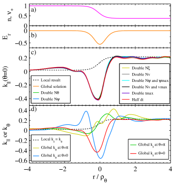
Figure 1: (Color online) a) Equilibrium density, normalized to its value at the left boundary. As $\nu_{*}$ happens to be 1 at this boundary and $T_{\mathrm{i}}\approx$ constant over the domain, this plot also gives the $\nu_{*}$ profile. b) Normalized radial electric field $-cI(v_{\mathrm{i}}B_{0})^{-1}d\Phi_{0}/d\psi$. c) The $dT_{\mathrm{i}}/d\psi$-driven parallel flow $k_{||}$ computed in the local approximation (dashed curve) differs from the global result (nearly indistinguishable solid curves) in the pedestal. The global code is well converged, demonstrated by changing each resolution parameter by $2\times$. d) Normalized poloidal flow $k_{\theta}$ and $k_{||}$, evaluated at the outboard ($\theta=0$) and inboard ($\theta=\pi$) midplanes.

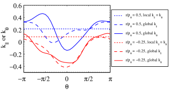
Figure 2: (Color online) Poloidal variation of the parallel flow coefficient $k_{||}$ and normalized poloidal flow $k_{\theta}$ at two radial locations straddling the pedestal.

To conclude, in this work we have demonstrated an extension of neoclassical calculations to a density pedestal with $r_{n}\sim\rho_{\theta}$ but $r_{T}\gg\rho_{\theta}$, retaining effects of finite orbit width, collisionality, and aspect ratio. The kinetic equation remains linear, and a $\delta f$ approach is possible. A numerical scheme was illustrated, demonstrating convergence on a laptop for experimentally relevant parameters. The Rosenbluth potentials are solved for along with the distribution function at each step, allowing use of the full linearized Fokker-Planck collision operator.

The analytic and numerical calculations show that in a pedestal, the plasma flow can differ significantly from the conventional prediction. While the poloidal flow is $\propto B_{\theta}$ in the core, the same is not generally true in the pedestal, and while the numerical coefficients in the parallel and poloidal flow are identical in conventional theory, in the pedestal these coefficients $k_{||}$ and $k_{\theta}$ are generally different. These modifications may be important for comparisons of experimental pedestal flows to theory.Marr K D, Lipschultz B, Catto P J, McDermott R M, Reinke M L and Simakov A N (2010) Two new contributions to mass conservation become important which are normally neglected: $\mbox{\boldmath$E$}\times\mbox{\boldmath$B$}$ motion of the perturbed density, and diamagnetic flow of the pressure perturbation. In general, the poloidal flow and $dT_{\mathrm{i}}/d\psi$ component of the parallel flow can differ in both magnitude and sign relative to local theory, as shown in the figures.

Associated with the modification to the flow, the usual division of the parallel current into Pfirsch-Schlüter and Ohmic-bootstrap components is changed (Eq. (11)), and the $dT_{\mathrm{i}}/d\psi$ contribution to the bootstrap current is altered. In the weak-$T_{\mathrm{i}}^{\prime}$ orderings used here, the associated terms are necessarily smaller than adjacent $dp/d\psi$ terms. However, analogous modifications to the current would presumably occur in a full-$f$ calculation when $r_{T}\sim\rho_{\theta}$, giving order-unity departures from local theory in that case.

We are grateful to Peter Catto and Felix Parra for enlightening discussions and for reading the manuscript. We also thank S. Kai Wong and Vincent Chan for assistance with benchmarking our local code to that of Ref. Wong S K and Chan V S, 2011. This work was supported by the Fusion Energy Postdoctoral Research Program administered by the Oak Ridge Institute for Science and Education.

References

Hinton, F. L., and Hazeltine, R.
D. (1976)Hinton, F. L., and
Hazeltine, R. D., Rev. Mod. Phys. 48, 239 (1976).
P. Helander and D. J. Sigmar (2002)P. Helander and D. J.
Sigmar, Collisional Transport in
Magnetized Plasmas (Cambridge University Press, Cambridge, 2002).
Sauter O, Harvey R W and Hinton F
L (1994)Sauter O, Harvey R W
and Hinton F L, Contrib. Plasma Phys. 34, 169 (1994).
Houlberg W A, Shaing K C, Hirshman S P and
Zarnstorff M C (1997)Houlberg W A, Shaing K
C, Hirshman S P and Zarnstorff M C, Phys. Plasmas 4, 3230 (1997).
Ernst D R, Bell M G, Bell R E, Bush C E, Chang Z,
Fredrickson E, Grisham L R, Hill K W, Jassby D L, Mansfield D K, McCune D C,
Park H K, Ramsey A T, Scott D S, Strachan J D, Synakowski E J, Taylor G,
Thompson M and Weiland R M (1998)Ernst D R, Bell M G,
Bell R E, Bush C E, Chang Z, Fredrickson E, Grisham L R, Hill K W, Jassby D
L, Mansfield D K, McCune D C, Park H K, Ramsey A T, Scott D S, Strachan J D,
Synakowski E J, Taylor G, Thompson M and Weiland R M, Phys. Plasmas 5, 665 (1998).
Belli E A and Candy J (2008)Belli E A and Candy
J, Theory of
Fusion Plasmas, Joint Varenna-Lausanne Intl. Workshop , CP1069 (2008).
Wong S K and Chan V S (2011)Wong S K and Chan V
S, Plasma
Phys. Controlled Fusion 53, 095005 (2011).
Lyons B C, Jardin S C, and Ramos J
J (2011)Lyons B C, Jardin S C,
and Ramos J J, Bull. Am. Phys. Soc 56, JP9.146 (2011).
Lin Z, Tang W M and Lee W W (1995)Lin Z, Tang W M and
Lee W W, Phys.
Plasmas 2, 2975
(1995).
Wang W X, Hinton F L and Wong S K (2001)Wang W X, Hinton F L
and Wong S K, Phys. Rev. Lett. 87, 055002 (2001).
Chang C S, Ku S and Weitzner H (2004)Chang C S, Ku S and
Weitzner H, Phys. Plasmas 11, 2649
(2004).
Vernay T, Brunner S, Villard L, McMillan B F,
Jollier S, Tran T M, Bottino A and Graves J P (2010)Vernay T, Brunner S,
Villard L, McMillan B F, Jollier S, Tran T M, Bottino A and Graves J P, Phys. Plasmas 17, 122301 (2010).
Xu X Q, Xiong Z, Dorr M R, Hittinger J A, Bodi K,
Candy J, Cohen B I, Cohen R H, Colella P, Kerbel G D, Krasheninnikov S,
Nevins W M, Qin H, Rognlien T D, Snyder P B and Umansky M V (2007)Xu X Q, Xiong Z, Dorr
M R, Hittinger J A, Bodi K, Candy J, Cohen B I, Cohen R H, Colella P, Kerbel
G D, Krasheninnikov S, Nevins W M, Qin H, Rognlien T D, Snyder P B and
Umansky M V, Nucl. Fusion 47, 809
(2007).
Cohen R H, Dorf M, Compton J C, Dorr M, Rognlien T
D, Colella P, McCorquodale P, Angus J and Krasheninnikov S (2012)Cohen R H, Dorf M,
Compton J C, Dorr M, Rognlien T D, Colella P, McCorquodale P, Angus J and
Krasheninnikov S, Bull. Am. Phys. Soc 57, BAPS.2012.APR.S1.38 (2012).
Kagan, G. and Catto, P.
J. (2010a)Kagan, G. and Catto,
P. J., Plasma
Phys. Controlled Fusion 52, 055004 (2010a).
Kagan, G. and Catto, P.
J. (2010b)Kagan, G. and Catto,
P. J., Phys.
Rev. Lett. 105, 045002
(2010b).
I. Pusztai, and P. J. Catto (2010)I. Pusztai, and P. J.
Catto, Plasma
Phys. Controlled Fusion 52, 075016 (2010).
Catto P J and Tsang K T (1977)Catto P J and Tsang K
T, Phys.
Fluids 20, 396 (1977).
Li B and Ernst D R (2011)Li B and Ernst D R
, Phys. Rev.
Lett. 106, 195002
(2011).
Hazeltine, R. (1973)Hazeltine, R., Plasma Phys. 15, 77 (1973).
Sauter O, Angioni C, and Lin-Liu Y
R (1999)Sauter O, Angioni C,
and Lin-Liu Y R, Phys. Plasmas 6, 2834 (1999).
Rosenbluth M N, MacDonald W M and Judd D
L (1957)Rosenbluth M N,
MacDonald W M and Judd D L, Phys. Rev. Lett. 107, 1 (1957).
Lapillonne X, McMillan B F, Gorler T, Brunner S,
Dannert T, Jenko F, Merz F and Villard L (2010)Lapillonne X, McMillan
B F, Gorler T, Brunner S, Dannert T, Jenko F, Merz F and Villard L, Phys. Plasmas 17, 112321 (2010).
Marr K D, Lipschultz B, Catto P J, McDermott R M,
Reinke M L and Simakov A N (2010)Marr K D, Lipschultz
B, Catto P J, McDermott R M, Reinke M L and Simakov A N, Plasma Phys. Controlled Fusion 52, 055010 (2010).