Gravitational Recoil of Inspiralling Black-Hole Binaries
to Second Post-Newtonian Order

Abstract

The loss of linear momentum by gravitational radiation and the resulting gravitational recoil of black-hole binary systems may play an important role in the growth of massive black holes in early galaxies. We calculate the gravitational recoil of non-spinning black-hole binaries at the second post-Newtonian order (2PN) beyond the dominant effect, obtaining, for the first time, the 1.5PN correction term due to tails of waves and the next 2PN term. We find that the maximum value of the net recoil experienced by the binary due to the inspiral phase up to the innermost stable circular orbit (ISCO) is of the order of $22\,\mathrm{km\,s}^{-1}$. We then estimate the kick velocity accumulated during the plunge from the ISCO up to the horizon by integrating the momentum flux using the 2PN formula along a plunge geodesic of the Schwarzschild metric. We find that the contribution of the plunge dominates over that of the inspiral. For a mass ratio $m_{2}/m_{1}=1/8$, we estimate a total recoil velocity (due to both adiabatic and plunge phases) of $100\pm 20\,\mathrm{km\,s^{-1}}$. For a ratio 0.38, the recoil is maximum and we estimate it to be $250\pm 50\,\mathrm{km\,s^{-1}}$. In the limit of small mass ratio, we estimate $V/c\approx 0.043\,(1\pm 20\%)\,(m_{2}/m_{1})^{2}$. Our estimates are consistent with, but span a substantially narrower range than, those of Favata et al. (2004).

1 Introduction and summary

The gravitational recoil of a system in response to the anisotropic emission of gravitational waves is a phenomenon with potentially important astrophysical consequences (Merritt et al., 2004). Specifically, in models for massive black hole formation involving successive mergers from smaller black hole seeds, a recoil with a velocity sufficient to eject the system from the host galaxy or mini-halo would effectively terminate the process. Recoils could eject coalescing black holes from dwarf galaxies or globular clusters. Even in galaxies whose potential wells are deep enough to confine the recoiling system, displacement of the system from the center could have important dynamical consequences for the galactic core. Consequently, it is important to have a robust estimate for the recoil velocity from inspiraling black hole binaries.

Recently, Favata et al. (2004) estimated the kick velocity for inspirals of both non-spinning and spinning black holes. For example, for non-spinning holes, with a mass ratio of 1:8, they estimated kick velocities between $20$ and $200\,\mathrm{km\,s^{-1}}$. The result was obtained by (i) making an estimate of the kick velocity accumulated during the adiabatic inspiral of the system up to its innermost stable circular orbit (ISCO), calculated using black-hole perturbation theory (valid in the small mass ratio limit), extended to finite mass ratios using scaling results from the quadrupole approximation, and (ii) combining that with a crude estimate of the kick velocity accumulated during the plunge phase (from the ISCO up to the horizon). The plunge contribution generally dominates the recoil, and is the most uncertain.

It is the purpose of this paper to compute more precisely the gravitational recoil velocity during the inspiral phase up to the ISCO, and to attempt to narrow that uncertainty in the plunge contribution for non-spinning inspiralling black holes.

Earlier approaches for computing the recoil of general matter systems include a near-zone computation of the recoil in linearized gravity (Peres, 1962), flux computations of the recoil as an interaction between the quadrupole and octupole moments (Bonnor & Rotenberg, 1961; Papapetrou, 1962), a general multipole expansion for the linear momentum flux (Thorne, 1980), and a radiation-reaction computation of the leading-order post-Newtonian recoil (Blanchet, 1997).

Using the post-Minkowskian and matching approach (Blanchet & Damour, 1986; Blanchet, 1995, 1998) for calculating equations of motion and gravitational radiation from compact binary systems in a post-Newtonian (PN) sequence, Blanchet et al. (2002, 2004) have derived the gravitational energy loss and phase to $\mathcal{O}[(v/c)^{7}]$ beyond the lowest-order quadrupole approximation, corresponding to 3.5PN order, and the gravitational wave amplitude to 2.5PN order (Arun et al., 2004). Using results from this program, we derive the linear momentum flux from compact binary inspiral to $\mathcal{O}[(v/c)^{4}]$, or 2PN order, beyond the lowest-order result.

The leading, “Newtonian” contribution  for binaries was first derived by Fitchett (1983), and was extended to 1PN order by Wiseman (1992). We extend these results by including both the 1.5PN order contributions caused by gravitational-wave tail effects, and the next 2PN order terms. We find that the linear momentum loss for binary systems in circular orbits is given by 

$$\frac{dP^{i}}{dt} = \frac{464}{105}\,\frac{\delta m}{m}\,\eta^{2}\,x^{11/2}\left[1+\left(-\frac{452}{87}-\frac{1139}{522}\eta\right)x+\frac{309}{58}\,\pi\,x^{3/2}\right.$$ (1)

$$\qquad\left.+\left(-\frac{71345}{22968}+\frac{36761}{2088}\eta+\frac{147101}{68904}\eta^{2}\right)x^{2}\right]{\hat{\lambda}}^{i}\,,$$

where $m=m_{1}+m_{2}$, $\delta m=m_{1}-m_{2}$, $\eta=m_{1}m_{2}/m^{2}$ (we have $0<\eta\leq 1/4$, with $\eta=1/4$ for equal masses), and where $x=(m\,\omega)^{2/3}$ is the PN parameter of the order of $\mathcal{O}[(v/c)^{2}]$, where $\omega=d\phi/dt$ is the orbital angular velocity. The quantity ${\hat{\lambda}}^{i}$ is a unit tangential vector directed in the same sense as the orbital velocity ${\bf v}={\bf v}_{1}-{\bf v}_{2}$. The term at order $x^{3/2}=\mathcal{O}[(v/c)^{3}]$ comes from gravitational-wave tails. Notice that, as expected for non-spinning systems, the flux vanishes for equal-mass systems ($\delta m=0$ or $\eta=1/4$).

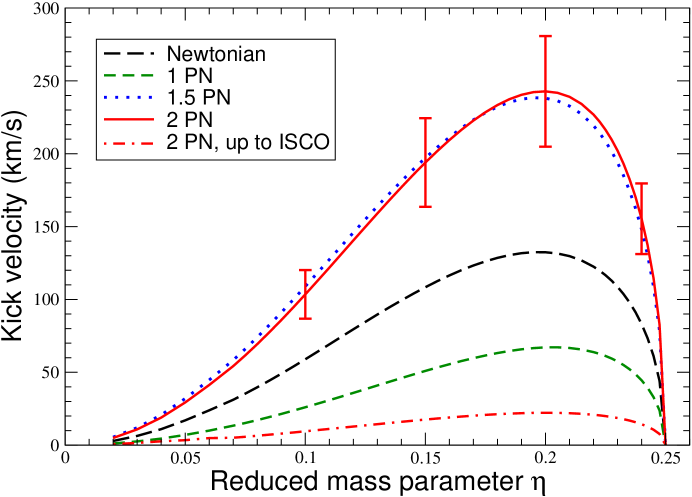
Figure 1: Recoil velocity as a function of $\eta$.

To calculate the net recoil velocity, we integrate this flux along a sequence of adiabatic quasi-circular inspiral orbits up to the ISCO. We then connect that orbit to an unstable inspiral orbit of a test body with mass $\mu=\eta\,m$ in the geometry of a Schwarzschild black hole of mass $m$, with initial conditions that include the effects of gravitational radiation damping. Using an integration variable that is regular all the way to the event horizon of the black hole, we integrate the momentum flux vector over the plunge orbit. Combining the adiabatic and plunge contributions, calculating the magnitude, and dividing by $m$ gives the net recoil velocity. Figure 1 shows the results. Plotted as a function of the reduced mass parameter $\eta$ are curves showing the results correct to Newtonian order, to 1PN order, to 1.5PN order and to 2PN order. Also shown is the contribution of the adiabatic part corresponding to the inspiral up to the ISCO (calculated to 2PN order). The “error bars” shown are an attempt to assess the accuracy of the result by including 2.5PN and 3PN terms with numerical coefficients that are allowed to range over values between $-10$ and $10$.

We note that the 1PN result is smaller than the Newtonian result because of the rather large negative coefficient seen in Eq. (1). On the other hand, the tail term at 1.5PN order plays a crucial role in increasing the magnitude of the effect (both for the adiabatic and plunge phases), and we observe that the small 2PN coefficient in Eq. (1) leads to the very small difference between the 1.5PN and 2PN curves in Fig. 1. In our opinion this constitutes a good indication of the “convergence” of the result. The momentum flux vanishes for the equal-mass case, $\eta=1/4$, and reaches a maximum around $\eta=0.2$ (a mass ratio of $0.38$), which corresponds to the maximum of the overall factor $\eta^{2}\delta m/m=\eta^{2}\sqrt{1-4\eta}$, reflecting the relatively weak dependence on $\eta$ in the PN corrections. We propose in Eq. (36) below a phenomenological analytic formula which embodies this weak $\eta$ dependence, and fits our 2PN curve remarkably well.

In contrast to the range 20 – 200 $\mathrm{km\,s^{-1}}$ for $\eta=0.1$ estimated by Favata et al. (2004), we estimate a recoil velocity of $100\pm 20\,\mathrm{km\,s^{-1}}$ for this mass ratio. For $\eta=0.2$ we estimate a recoil between $200$ and $300\,\mathrm{km\,s^{-1}}$, with a “best guess” of $250\,\mathrm{km\,s^{-1}}$ (the maximum velocity shown in Fig. 1 is $243\,\mathrm{km\,s^{-1}}$). We regard our computation of the recoil in the adiabatic inspiral phase (up to the ISCO) as rather solid thanks to the accurate 2PN formula we use, and the fact that the 1.5PN and 2PN results are so close to each other. However, obviously, using PN methods to study binary inspiral inside the ISCO is not without risks, and so it would be very desirable to see a check of our estimates using either black hole perturbation theory (along the lines of Oohara & Nakamura (1983), Nakamura & Haugan (1983) or Fitchett & Detweiler (1984)) or full numerical relativity. It is relevant to point out that our estimates agree well with those obtained using numerical relativity in the “Lazarus approach”, or close-limit approximation, which treats the final merger of comparable-mass black holes using a hybrid method combining numerical relativity with perturbation theory (Campanelli, 2005). In the small mass-ratio limit, they also agree well with a calculation of the recoil from the head-on plunge from infinity using perturbation theory (Nakamura et al., 1987). Therefore, we hope that our estimates will enable a more focussed discussion of the astrophysical consequences of gravitational radiation recoil.

The remainder of this paper provides details. In Section 2, we derive the 2PN accurate linear momentum flux using a multipole decomposition, together with 2PN expressions for the multipole moments in terms of source variables. In Section 3 we specialize to binary systems, and to circular orbits. In Section 4, we use these results to estimate the recoil velocity and discuss various checks of our estimates. Section 5 makes concluding remarks.

2 General formulae for linear momentum flux

The flux of linear momentum $\mathbf{P}$, carried away from general isolated sources, is first expressed in terms of symmetric and trace-free (STF) radiative multipole moments, which constitute very convenient sets of observables parametrizing the asymptotic wave form at the leading order $|\mathbf{X}|^{-1}$ in the distance to the source, in an appropriate radiative coordinate system $X^{\mu}=(T,\mathbf{X})$ (Thorne, 1980). Denoting by $U_{i_{1}\cdots i_{\ell}}(T)$ and $V_{i_{1}\cdots i_{\ell}}(T)$ the mass-type and current-type radiative moments at radiative coordinate time $T$ (where $\ell$ is the multipolar order), the linear momentum flux reads

$$\mathcal{F}^{i}_{\mathbf{P}}(T) = \sum_{\ell=2}^{+\infty}\left\{\frac{2(\ell+2)(\ell+3)}{\ell(\ell+1)!(2\ell+3)!!}\,U_{ii_{1}\cdots i_{\ell}}^{(1)}(T)\,U_{i_{1}\cdots i_{\ell}}^{(1)}(T)\right.$$ (2)

$$\qquad\left.+\frac{8(\ell+2)}{(\ell-1)(\ell+1)!(2\ell+1)!!}\,\varepsilon_{ijk}\,U_{ji_{1}\cdots i_{\ell-1}}^{(1)}(T)\,V_{ki_{1}\cdots i_{\ell-1}}^{(1)}(T)\right.$$

$$\qquad\left.+\frac{8(\ell+3)}{(\ell+1)!(2\ell+3)!!}\,V_{ii_{1}\cdots i_{\ell}}^{(1)}(T)\,V_{i_{1}\cdots i_{\ell}}^{(1)}(T)\right\}\,,$$

where the superscript $(n)$ refers to the time-derivatives, and $\varepsilon_{ijk}$ is Levi-Civita’s antisymmetric symbol, such that $\varepsilon_{123}=+1$. Taking into account all terms up to relative 2PN order (in the case of slowly moving, PN sources), we obtain

$$\mathcal{F}^{i}_{\mathbf{P}} = \frac{2}{63}\,U_{ijk}^{(1)}\,U_{jk}^{(1)}+\frac{16}{45}\,\varepsilon_{ijk}\,U_{jl}^{(1)}\,V_{kl}^{(1)}$$ (3)

$$+ \frac{1}{1134}\,U_{ijkl}^{(1)}\,U_{jkl}^{(1)}+\frac{1}{126}\,\varepsilon_{ijk}\,U_{jlm}^{(1)}\,V_{klm}^{(1)}+\frac{4}{63}\,V_{ijk}^{(1)}\,V_{jk}^{(1)}$$

$$+ \frac{1}{59400}\,U_{ijklm}^{(1)}\,U_{jklm}^{(1)}+\frac{2}{14175}\,\varepsilon_{ijk}\,U_{jlmn}^{(1)}\,V_{klmn}^{(1)}+\frac{2}{945}\,V_{ijkl}^{(1)}\,V_{jkl}^{(1)}\,.$$

The first two terms represent the leading order in the linear momentum flux, which corresponds to radiation reaction effects in the source’s equations of motion occuring at the 3.5PN order with respect to the Newtonian force law. Indeed, recall that although the dominant radiation reaction force is at 2.5PN order, the total integrated radiation reaction force on the system (which gives the linear momentum loss or recoil) starts only at the next 3.5PN order (Peres, 1962; Bonnor & Rotenberg, 1961; Papapetrou, 1962). Radiation reaction terms at the 3.5PN level for compact binaries in general orbits have been computed by Iyer & Will (1995), Jaranowski & Schäfer (1997), Pati & Will (2002), Königsdörffer et al. (2003) and Nissanke & Blanchet (2005). In Eq. (3) all the terms up to 2PN order relative to the leading linear momentum flux are included. This precision corresponds formally to radiation reaction effects up to 5.5PN order.

The radiative multipole moments, seen at (Minkowskian) future null infinity, $U_{i_{1}\cdots i_{\ell}}$ and $V_{i_{1}\cdots i_{\ell}}$, are now related to the source multipole moments, say $I_{i_{1}\cdots i_{\ell}}$ and $J_{i_{1}\cdots i_{\ell}}$, following the post-Minkowskian and matching approach of Blanchet & Damour (1986) and Blanchet (1995, 1998). The radiative moments differ from the source moments by non-linear multipole interactions. At the relative 2PN order considered in the present paper, the difference is only due to interactions of the mass monopole $M$ of the source with higher moments, so-called gravitational-wave tail effects. For the source moments $I_{i_{1}\cdots i_{\ell}}$ and $J_{i_{1}\cdots i_{\ell}}$, we use the expressions obtained in Blanchet (1995, 1998), valid for a general extended isolated PN source. These moments are the analogues of the multipole moments originally introduced by Epstein & Wagoner (1975) and generalized by Thorne (1980), and which constitute the building blocks of the direct integration of the retarded Einstein equations (DIRE) formalism (Will & Wiseman, 1996; Pati & Will, 2000). The radiative moments appearing in Eq. (3) are given in terms of the source moments by (see Eqs. (4.35) in Blanchet (1995))

$$U_{ij}(T) = I^{(2)}_{ij}(T)+2\,M\int_{-\infty}^{T}d\tau\,I^{(4)}_{ij}(\tau)\left[\ln\left(\frac{T-\tau}{2b}\right)+\frac{11}{12}\right]\,,$$ (4a)

$$U_{ijk}(T) = I^{(3)}_{ijk}(T)+2\,M\int_{-\infty}^{T}d\tau\,I^{(5)}_{ijk}(\tau)\left[\ln\left(\frac{T-\tau}{2b}\right)+\frac{97}{60}\right]\,,$$ (4b)

$$V_{ij}(T) = J^{(2)}_{ij}(T)+2\,M\int_{-\infty}^{T}d\tau\,J^{(4)}_{ij}(\tau)\left[\ln\left(\frac{T-\tau}{2b}\right)+\frac{7}{6}\right]\,,$$ (4c)

where $M\equiv I$ denotes the constant mass monopole or total ADM mass of the source. The relative order of the tail integrals in Eqs. (4) is 1.5PN. The constant $b$ entering the logarithmic kernel of the tail integrals represents an arbitrary scale which is defined by

$$T=t_{\mathrm{H}}-\rho_{\mathrm{H}}-2\,M\ln\left(\frac{\rho_{\mathrm{H}}}{b}\right)\,,$$ (5)

where $t_{\mathrm{H}}$ and $\rho_{\mathrm{H}}$ correspond to a harmonic coordinate chart covering the local isolated source ($\rho_{\mathrm{H}}$ is the distance of the source in harmonic coordinates). We insert Eqs. (4) into the linear momentum flux (3) and naturally decompose it into

$$\mathcal{F}^{i}_{\mathbf{P}}=\left(\mathcal{F}^{i}_{\mathbf{P}}\right)_{\mathrm{inst}}+\left(\mathcal{F}^{i}_{\mathbf{P}}\right)_{\mathrm{tail}}\,,$$ (6)

where the “instantaneous” piece, which depends on the state of the source only at time $T$, is given by

$$\left(\mathcal{F}^{i}_{\mathbf{P}}\right)_{\mathrm{inst}} = \frac{2}{63}\,I_{ijk}^{(4)}\,I_{jk}^{(3)}+\frac{16}{45}\,\varepsilon_{ijk}\,I_{jl}^{(3)}\,J_{kl}^{(3)}$$ (7)

$$+ \frac{1}{1134}\,I_{ijkl}^{(5)}\,I_{jkl}^{(4)}+\frac{1}{126}\,\varepsilon_{ijk}\,I_{jlm}^{(4)}\,J_{klm}^{(4)}+\frac{4}{63}\,J_{ijk}^{(4)}\,I_{jk}^{(3)}$$

$$+ \frac{1}{59400}\,I_{ijklm}^{(6)}\,I_{jklm}^{(5)}+\frac{2}{14175}\,\varepsilon_{ijk}\,I_{jlmn}^{(5)}\,J_{klmn}^{(5)}+\frac{2}{945}\,J_{ijkl}^{(5)}\,I_{jkl}^{(4)}\,,$$

and the “tail” piece, formally depending on the integrated past of the source, reads

$$\left(\mathcal{F}^{i}_{\mathbf{P}}\right)_{\mathrm{tail}} = \frac{4\,M}{63}\,I_{ijk}^{(4)}(T)\int_{-\infty}^{T}d\tau\,I_{jk}^{(5)}(\tau)\left[\ln\left(\frac{T-\tau}{2b}\right)+\frac{11}{12}\right]$$ (8)

$$+ \frac{4\,M}{63}\,I_{jk}^{(3)}(T)\int_{-\infty}^{T}d\tau\,I_{ijk}^{(6)}(\tau)\left[\ln\left(\frac{T-\tau}{2b}\right)+\frac{97}{60}\right]$$

$$+ \frac{32\,M}{45}\,\varepsilon_{ijk}\,I_{jl}^{(3)}(T)\int_{-\infty}^{T}d\tau\,J_{kl}^{(5)}(\tau)\left[\ln\left(\frac{T-\tau}{2b}\right)+\frac{7}{6}\right]$$

$$+ \frac{32\,M}{45}\varepsilon_{ijk}J_{kl}^{(3)}(T)\int_{-\infty}^{T}d\tau\,I_{jl}^{(5)}(\tau)\left[\ln\left(\frac{T-\tau}{2b}\right)+\frac{11}{12}\right]\,.$$

The four terms in Eq. (8) correspond to the tail parts of the moments parametrizing the “Newtonian” approximation to the flux given by the first line of (3). All of them will contribute at 1.5PN order.

3 Application to compact binary systems

We specialize the expressions given in Section 2, which are valid for general PN sources, to the case of compact binary systems modelled by two point masses $m_{1}$ and $m_{2}$. For this application, all the required source multipole moments up to 2PN order admit known explicit expressions, computed in Blanchet et al. (1995, 2002) and Arun et al. (2004) for circular binary orbits. Here we quote only the results. Mass parameters are $m=m_{1}+m_{2}$, $\delta m=m_{1}-m_{2}$ and the symmetric mass ratio $\eta=m_{1}m_{2}/m^{2}$. We define $\mathbf{x}\equiv\mathbf{x}_{1}-\mathbf{x}_{2}$ and $r\equiv|\mathbf{x}|$ to be the relative vector and separation between the particles in harmonic coordinates, respectively, and $\mathbf{v}\equiv d\mathbf{x}/dt$ to be their relative velocity ($t\equiv t_{\mathrm{H}}$ is the harmonic coordinate time). We have, for mass-type moments,

$$I_{ij} = \eta\,m\left\{{x}^{\langle ij\rangle}\left[1+\frac{m}{r}\left(-\frac{1}{42}-\frac{13}{14}\eta\right)+\left(\frac{m}{r}\right)^{2}\left(-\frac{461}{1512}-\frac{18395}{1512}\eta-\frac{241}{1512}\eta^{2}\right)\right]\right.$$ (9a)

$$~{}~{}\left.+\,r^{2}v^{\langle ij\rangle}\left[\frac{11}{21}-\frac{11}{7}\eta+\frac{m}{r}\left(\frac{1607}{378}-\frac{1681}{378}\eta+\frac{229}{378}\eta^{2}\right)\right]\right\}\,,$$

$$I_{ijk} = -\eta\,\delta m\,\left\{{x}^{\langle ijk\rangle}\left[1-\frac{m}{r}\eta-\left(\frac{m}{r}\right)^{2}\left(\frac{139}{330}+\frac{11923}{660}\eta+\frac{29}{110}\eta^{2}\right)\right]\right.$$ (9b)

$$~{}~{}+r^{2}\,x^{\langle i}v^{jk\rangle}\left[1-2\eta-\frac{m}{r}\left(-\frac{1066}{165}+\left.\frac{1433}{330}\eta-\frac{21}{55}\eta^{2}\right)\right]\right\}\,,$$

$$I_{ijkl} = \eta\,m\,\left\{x^{\langle ijkl\rangle}\left[1-3\eta+\frac{m}{r}\left(\frac{3}{110}-\frac{25}{22}\eta+\frac{69}{22}\eta^{2}\right)\right]\right.$$ (9c)

$$~{}~{}+\left.\frac{78}{55}\,r^{2}\,v^{\langle ij}x^{kl\rangle}(1-5\eta+5\eta^{2})\right\}\,,$$

$$I_{ijklm} = -\eta\,\delta m\,x^{\langle ijklm\rangle}\left(1-2\eta\right)\,,$$ (9d)

and, for current-type moments,

$$J_{ij} = -\eta\,\delta m\left\{\varepsilon^{ab\langle i}x^{j\rangle a}v^{b}\left[1+\frac{m}{r}\left(\frac{67}{28}-\frac{2}{7}\eta\right)\right.\right.$$ (10a)

$$~{}~{}\left.\left.+\left(\frac{m}{r}\right)^{2}\left(\frac{13}{9}-\frac{4651}{252}\eta-\frac{1}{168}\eta^{2}\right)\right]\right\}\,,$$

$$J_{ijk} = \eta\,m\left\{\varepsilon^{ab\langle i}x^{jk\rangle a}v^{b}\left[1-3\eta+\frac{m}{r}\left(\frac{181}{90}-\frac{109}{18}\eta+\frac{13}{18}\eta^{2}\right)\right]\right.$$ (10b)

$$~{}~{}+\left.\frac{7}{45}\,r^{2}\,\varepsilon^{ab\langle i}v^{jk\rangle b}x^{a}(1-5\eta+5\eta^{2})\right\}\,,$$

$$J_{ijkl} = -\eta\,\delta m\,\varepsilon^{ab\langle i}x^{jkl\rangle a}v^{b}\left(1-2\eta\right)\,.$$ (10c)

We indicate the symmetric-trace-free projection using carets surrounding indices. Thus, the STF product of $\ell$ spatial vectors, say $x^{i_{1}\cdots i_{\ell}}=x^{i_{1}}\cdots x^{i_{\ell}}$, is denoted $x^{\langle i_{1}\cdots i_{\ell}\rangle}=\mathrm{STF}\left[x^{i_{1}\cdots i_{\ell}}\right]$. Similarly, we pose $x^{\langle i_{1}\cdots i_{k}}v^{i_{k+1}\cdots i_{\ell}\rangle}=\mathrm{STF}\left[x^{i_{1}\cdots i_{k}}v^{i_{k+1}\cdots i_{\ell}}\right]$.

The total mass $M$ in front of the tail integrals in (4) simply reduces, at the approximation considered in this paper, to the sum of the masses, i.e. $M=m=m_{1}+m_{2}$. Thus, to compute the tail contributions (8), we simply need the Newtonian approximation for all the moments.

As seen in Eqs. (7)– (8) we need to perform repeated time-differentiations of the moments. These are consistently computed using for the replacement of accelerations the binary’s 2PN equations of motion in harmonic coordinates (for circular 2PN orbits)

$$\frac{dv^{i}}{dt}=-\omega^{2}x^{i}\,,$$ (11)

where $\omega$ denotes the angular frequency of the circular motion, which is related to the orbital separation $r$ by the generalized Kepler law

$$\omega^{2}=\frac{m}{r^{3}}\biggl{\{}1+\frac{m}{r}(-3+\eta)+\left(\frac{m}{r}\right)^{2}\left(6+\frac{41}{4}\eta+\eta^{2}\right)\biggr{\}}\,.$$ (12)

The inverse of this law yields [using $x\equiv(m\,\omega)^{2/3}$]

$$\frac{m}{r}=x\,\biggl{\{}1+x\,\left(1-\frac{\eta}{3}\right)+x^{2}\,\left(1-\frac{65}{12}\eta\right)\biggr{\}}\,.$$ (13)

The tail integrals of Eq. (8) are computed in the adiabatic approximation by substituting into the integrands the components of the moments calculated for exactly circular orbits, with the current value of the orbital frequency $\omega$ (at time $T$), but with different phases corresponding to whether the moment is evaluated at the current time $T$ or at the retarded time $\tau<T$. For exactly circular orbits the phase difference is simply $\Delta\phi=\omega(T-\tau)$. All the contractions of indices are performed, and the result is obtained in the form of a sum of terms which can all be analytically computed by means of the mathematical formula

$$\int_{0}^{+\infty}d\tau\,\ln\left(\frac{\tau}{2b}\right)\,e^{\mathrm{i}\,n\,\omega\,\tau}=-\frac{1}{n\,\omega}\left\{\frac{\pi}{2}+\mathrm{i}\Bigl{[}\ln\left(2n\,\omega\,b\right)+C\Bigr{]}\right\}\,,$$ (14)

where $\omega$ is the orbital frequency, $n$ the number of the considered harmonics of the signal ($n=1$, $2$ or $3$ at the present 2PN order) and $C=0.577\cdots$ is Euler’s constant. As shown in Blanchet & Schäfer (1993) (see also Blanchet et al. (1995); Arun et al. (2004)), this procedure to compute the tails is correct in the adiabatic limit, i.e. modulo the neglect of 2.5PN radiation reaction terms $\mathcal{O}[(v/c)^{5}]$ which do not contribute at the present order.

As it will turn out, the effect of tails in the linear momentum flux comes only from the first term in the right side of Eq. (14), proportional to $\pi$. All the contributions due to the second term in (14), which involves the logarithm of frequency, can be reabsorbed into a convenient definition of the phase variable, and then shown to correspond to a very small phase modulation which is negligible at the present PN order. This possibility of introducing a new phase variable containing all the logarithms of frequency was usefully applied in previous computations of the binary’s polarization waveforms (Blanchet et al., 1996; Arun et al., 2004). We introduce the phase variable $\psi$ differing from the actual orbital phase angle $\phi$, whose time derivative equals the orbital frequency ($\dot{\phi}=\omega$), by

$$\psi=\phi-2m\,\omega\ln\left(\frac{\omega}{\widehat{\omega}}\right)\,,$$ (15)

where $\widehat{\omega}$ denotes a certain constant frequency scale that is related to the constant $b$ which was introduced into the tail integrals (4), and parametrizes the coordinate transformation (5) between harmonic and radiative coordinates. The constants $\widehat{\omega}$ and $b$ are in fact devoid of any physical meaning and can be chosen at will (Blanchet et al., 1996; Arun et al., 2004). To check this let us use the time dependence of the orbital phase $\phi$ due to radiation-reaction inspiral in the adiabatic limit, given at the lowest quadrupolar order by (see e.g. Blanchet et al. (1996))

$$\phi_{c}-\phi(T)=\frac{1}{\eta}\left(\frac{\eta}{5m}[T_{c}-T]\right)^{5/8}\,,$$ (16)

where $T_{c}$ and $\phi_{c}$ denote the instant of coalescence and the value of the phase at that instant. Then it is easy to verify that an arbitrary rescaling of the constant $\widehat{\omega}$ by $\widehat{\omega}\rightarrow\lambda\,\widehat{\omega}$ simply corresponds to a constant shift in the value of the instant of coalescence, namely $T_{c}\rightarrow T_{c}+2m\,\ln\lambda$. Thus, any choice for $\widehat{\omega}$ is in fact irrelevant since it is equivalent to a choice of the origin of time in the wave zone. The relation between $\widehat{\omega}$ and $b$ is given here for completeness,

$$\widehat{\omega}=\frac{1}{b}\,\mathrm{exp}\!\left[\frac{5921}{1740}+\frac{48}{29}\ln 2-\frac{405}{116}\ln 3-C\right]\,.$$ (17)

The irrelevance of $\widehat{\omega}$ and $b$ is also clear from Eq. (5) where one sees that they correspond to an adjustement of the time origin of radiative coordinates with respect to that of the source-rooted harmonic coordinates.

Let us next point out that the phase modulation of the log-term in Eq. (15) represents in fact a very small effect, which is formally of order 4PN relative to the dominant radiation-reaction expression of the phase as a function of time, given by (16). This is clear from the fact that Eq. (16) is of the order of the inverse of radiation-reaction effects, which can be said to correspond to $-$2.5PN order, and that, in comparison, the tail term is of order +1.5PN, which means 4PN relative order. In the present paper we shall neglect such 4PN effects and will therefore identify the phase $\psi$ with the actual orbital phase of the binary.

We introduce two unit vectors $\hat{n}^{i}$ and $\hat{\lambda}^{i}$, respectively along the binary’s separation, i.e. in the direction of the phase angle $\psi$, and along the relative velocity, in the direction of $\psi+\frac{\pi}{2}$, namely

$$\hat{n}^{i}=\left(\begin{array}[]{c}\cos\psi\\ \sin\psi\\ 0\end{array}\right)~{}~{}\,\rm{and}\,~{}~{}\hat{\lambda}^{i}=\left(\begin{array}[]{c}-\sin\psi\\ \cos\psi\\ 0\end{array}\right).$$ (18)

Finally, the reduction of the two terms (7) and (8) for compact binaries using the source moments (9)–(10) is straightforward, and yields the complete expression of the 2PN linear momentum flux,

$$\mathcal{F}^{i}_{\mathbf{P}} = -\frac{464}{105}\,\eta^{2}\,\frac{\delta m}{m}\left(\frac{m}{r}\right)^{11/2}\left[1+\left(-\frac{1861}{174}-\frac{91}{261}\eta\right)\frac{m}{r}+\frac{309}{58}\,\pi\left(\frac{m}{r}\right)^{3/2}\right.$$ (19)

$$\qquad\left.+\left(\frac{139355}{2871}+\frac{36269}{1044}\eta+\frac{17}{3828}\eta^{2}\right)\left(\frac{m}{r}\right)^{2}\right]\,\hat{\lambda}^{i}\,.$$

The first term is the “Newtonian” one which, as we noted above, really corresponds to a 3.5PN radiation reaction effect. It is followed by the 1PN relative correction, then the 1.5PN correction, proportional to $\pi$ and which is exclusively due to tails, and finally the 2PN correction term. We find that the 1PN term is in agreement with the previous result by Wiseman (1992). The tail term at order 1.5PN and the 2PN term are new with the present paper. Alternatively we can also express the flux in terms of the orbital frequency $\omega$, with the help of the PN parameter defined by $x=(m\,\omega)^{2/3}$. Using Eq. (13) we obtain

$$\mathcal{F}^{i}_{\mathbf{P}} = -\frac{464}{105}\,\frac{\delta m}{m}\,\eta^{2}\,x^{11/2}\left[1+\left(-\frac{452}{87}-\frac{1139}{522}\eta\right)x+\frac{309}{58}\,\pi\,x^{3/2}\right.$$ (20)

$$\qquad\left.+\left(-\frac{71345}{22968}+\frac{36761}{2088}\eta+\frac{147101}{68904}\eta^{2}\right)x^{2}\right]{\hat{\lambda}}^{i}\,.$$

The latter form is interesting because it remains invariant under a large class of gauge transformations.

Next, in order to obtain the local loss of linear momentum by the source, we apply the momentum balance equation

$$\frac{dP^{i}}{dT}=-\mathcal{F}^{i}_{\mathbf{P}}(T)\,,$$ (21)

which yields Eq. (1). Upon integration, this yields the net change of linear momentum, say $\Delta P^{i}=-\int_{-\infty}^{T}dt\,\mathcal{F}^{i}_{\mathbf{P}}(t)$. In the adiabatic limit, i.e. at any instant before the passage at the ISCO, the closed form of $\Delta P^{i}$ can be simply obtained (for circular orbits) from the fact that ${d\hat{n}^{i}}/{dt}=\omega\hat{\lambda}^{i}$ and the constancy of the orbital frequency $\omega$. This is of course correct modulo fractional error terms $\mathcal{O}[(v/c)^{5}]$ which are negligible here. So, integrating the balance equation (21) in the adiabatic approximation simply amounts to replacing the unit vector $\hat{\lambda}^{i}$ by $\hat{n}^{i}$ and dividing by the orbital frequency $\omega$. In this way we obtain the recoil velocity $V^{i}\equiv\Delta P^{i}/m$ as 

$$V^{i} = \frac{464}{105}\,\eta^{2}\,\frac{\delta m}{m}\left(\frac{m}{r}\right)^{4}\left[1+\left(-\frac{800}{87}-\frac{443}{522}\eta\right)\frac{m}{r}+\frac{309}{58}\,\pi\left(\frac{m}{r}\right)^{3/2}\right.$$ (22)

$$\qquad\left.+\left(\frac{754975}{22968}+\frac{67213}{2088}\eta+\frac{1235}{22968}\eta^{2}\right)\left(\frac{m}{r}\right)^{2}\right]\,\hat{n}^{i}\,,$$

or, alternatively, in terms of the $x$-parameter,

$$V^{i} = \frac{464}{105}\,\eta^{2}\,\frac{\delta m}{m}x^{4}\left[1+\left(-\frac{452}{87}-\frac{1139}{522}\eta\right)\,x+\frac{309}{58}\,\pi\,x^{3/2}\right.$$ (23)

$$\qquad\left.+\left(-\frac{71345}{22968}+\frac{36761}{2088}\eta+\frac{147101}{68904}\eta^{2}\right)\,x^{2}\right]\,\hat{n}^{i}\,.$$

Equations (1) and (23) will be the basis for our numerical estimates of the recoil velocity, to be carried out in the next Section.

4 Estimating the recoil velocity

4.1 Basic assumptions and analytic formulae

We now wish to use Eqs. (1) and (23) to estimate the recoil velocity that results from the inspiral and merger of two black holes. It is clear that the PN approximation becomes less reliable inside the innermost stable circular orbit (ISCO). Nevertheless, we have an expression that is accurate to 2PN order beyond the leading effect, which will therefore be very accurate over all the inspiral phase all the way down to the ISCO, so we have some hope that, if the higher-order terms can be seen to be small corrections throughout the process, we can make a robust estimate of the overall kick.

In Eq. (23) we have re-expressed the recoil velocity in terms of the orbital angular velocity $\omega$, Eq. (12), consistently to 2PN order. One advantage of this change of variables is that the momentum loss is now expressed in terms of a somewhat less coordinate dependent quantity, namely the orbital angular velocity as seen from infinity. A second advantage is that the convergence of the PN series is significantly improved. In terms of the variable $m/r$, the coefficients of the 1PN and 2PN terms are of order $-$10 and 33 – 41, respectively, depending on the value of $\eta$, whereas in terms of $x$, they are of order $-$5 and $-$3 – $+$1.4, respectively.

We assume that the system undergoes an adiabatic inspiral along a sequence of circular orbits up to the ISCO. For the present discussion the ISCO is taken to be the one for point-mass motion around a Schwarzschild black hole of mass $m=m_{1}+m_{2}$, namely $m\,\omega_{\mathrm{ISCO}}=6^{-3/2}$ or $x_{\mathrm{ISCO}}=1/6$. The recoil velocity at the ISCO is thus given by

$$V_{\mathrm{ISCO}}^{i} = \frac{464}{105}\,\frac{\delta m}{m}\,\eta^{2}\,x_{\mathrm{ISCO}}^{4}\left[1+\left(-\frac{452}{87}-\frac{1139}{522}\eta\right)x_{\mathrm{ISCO}}+\frac{309}{58}\,\pi\,x_{\mathrm{ISCO}}^{3/2}\right.$$ (24)

$$\qquad\left.+\left(-\frac{71345}{22968}+\frac{36761}{2088}\eta+\frac{147101}{68904}\eta^{2}\right)x_{\mathrm{ISCO}}^{2}\right]\hat{n}^{i}_{\mathrm{ISCO}}\,.$$

In order to determine the kick velocity accumulated during the plunge, we make a number of simplifying assumptions. We first assume that the plunge can be viewed as that of a “test” particle of mass $\mu$ moving in the fixed Schwarzschild geometry of a body of mass $m$, following the “effective one-body” approach of Buonanno & Damour (1999) and Damour (2001). We also assume that the effect on the plunge orbit of the radiation of energy and angular momentum may be ignored; over the small number of orbits that make up the plunge, this seems like a reasonable approximation (Favata et al. (2004) make the same assumption).

We therefore adopt the geodesic equations for the Schwarzschild geometry,

$$\frac{dt}{d\tau} = \frac{\tilde{E}}{1-{2m}/{r_{\mathrm{S}}}}\,,$$ (25a)

$$\frac{d\psi}{d\tau} = \frac{\tilde{L}}{r_{\mathrm{S}}^{2}}\,,$$ (25b)

$$\left(\frac{dr_{\mathrm{S}}}{d\tau}\right)^{2} = \tilde{E}^{2}-\left(1-\frac{2m}{r_{\mathrm{S}}}\right)\left[1+\frac{\tilde{L}^{2}}{r_{\mathrm{S}}^{2}}\right]\,,$$ (25c)

where $\tau$ is proper time along the geodesic, $\tilde{E}$ is the energy per unit mass ($\mu$ in this case), and $\tilde{L}\equiv m\,\bar{L}$ is the angular momentum per unit mass. Then, from Eqs. (25b) and (25c), we obtain the phase angle of the orbit $\psi$ as a function of $y=m/r_{\mathrm{S}}$ by

$$\psi=\int_{y_{0}}^{y}\left(\frac{\bar{L}^{2}}{\tilde{E}^{2}-(1-2y)(1+\bar{L}^{2}y^{2})}\right)^{1/2}dy\,,$$ (26)

where we choose $\psi=0$ at the beginning of the plunge orbit defined by $y=y_{0}$.

The kick velocity accumulated during the plunge is then given by

$$\Delta V^{i}_{\mathrm{plunge}}=\frac{1}{m}\int_{t_{0}}^{t_{\mathrm{Horizon}}}\frac{dP^{i}}{dt}dt\,.$$ (27)

However, the coordinate time $t$ is singular at the event horizon, so we must find a non-singular variable to carry out the integration. We choose the “proper” angular frequency, $\bar{\omega}=d\psi/d\tau$. In addition to being monotonically increasing, this variable has the following useful properties along the plunge geodesic:

$$m\,\bar{\omega} = \bar{L}\,y^{2}\,,$$ (28a)

$$m\,\omega = m\,\bar{\omega}\,\frac{1-2y}{\tilde{E}}=\frac{\bar{L}}{\tilde{E}}\,y^{2}(1-2y)\,,$$ (28b)

$$\frac{d\bar{\omega}}{dt} = \frac{2}{m}\,\omega\,y\Bigl{[}\tilde{E}^{2}-(1-2y)(1+\bar{L}^{2}y^{2})\Bigr{]}^{1/2}\,.$$ (28c)

Then

$$\Delta V^{i}_{\mathrm{plunge}} = \frac{1}{m}\int\frac{dP^{i}}{dt}\frac{d\bar{\omega}}{d\bar{\omega}/dt}$$ (29)

$$= \bar{L}\,\int_{y_{0}}^{y_{\mathrm{Horizon}}}\left(\frac{1}{m\,\omega}\frac{dP^{i}}{dt}\right)\frac{dy}{\Bigl{[}\tilde{E}^{2}-(1-2y)(1+\bar{L}^{2}y^{2})\Bigr{]}^{1/2}}\,,$$

where $y_{0}$ is defined by the matching to a circular orbit at the ISCO that we shall discuss below.

Notice that, because $dP^{i}/dt\propto x^{11/2}\propto(m\,\omega)^{11/3}$, the quantity in parentheses in Eq. (29) is well behaved at the horizon; in fact it vanishes at the horizon because $\omega=0$ there [cf. Eq. (28b)]. Thus, we find that the integrand of Eq. (29) behaves like $(m\,\omega)^{8/3}\propto(1-2y)^{8/3}$ at the horizon, and the integral is perfectly convergent. Furthermore, since the expansion of $dP^{i}/dt$ is in powers of $m\,\omega$, the convergence of the PN series is actually improved as the particle approaches the horizon. To carry out the integral, then, we substitute for $x=(m\,\omega)^{2/3}$ in $dP^{i}/dt$ using Eq. (28b), and integrate over $y$.

We regard this approach as robust, because it uses invariant quantities such as angular frequencies, and uses the nature of the flux formula itself to obtain an integral that is automatically convergent. Favata et al. (2004) tried to control the singular behavior of the $t$ integration with an ad hoc regularization scheme.

We then combine Eqs. (24) and (29) vectorially to obtain the net kick velocity,

$$\Delta V^{i}=V^{i}_{\mathrm{ISCO}}+\Delta V^{i}_{\mathrm{plunge}}\,,$$ (30)

in which $V^{i}_{\mathrm{ISCO}}$ is given by Eq. (24) above with $\hat{n}^{i}_{\mathrm{ISCO}}=(1,0,0)$.

There are many ways to match a circular orbit at the ISCO to a suitable plunge orbit; we use two different methods. In one, we give the particle an energy $\tilde{E}$ such that, at the ISCO, and for an ISCO angular momentum $\tilde{L}_{\mathrm{ISCO}}=\sqrt{12}\,m$, the particle has a radial velocity given by the standard quadrupole energy-loss formula for a circular orbit, namely $dr_{\mathrm{H}}/dt=-(64/5)\eta(m/r_{\mathrm{H}})^{3}$, where $r_{\mathrm{H}}$ is the orbital separation in harmonic coordinates. At the ISCO for a test body, $r_{\mathrm{H}}=5m$, so we have $(dr_{\mathrm{H}}/dt)_{\mathrm{ISCO}}=-(8/25)^{2}\eta$. This means also $(dr_{\mathrm{S}}/dt)_{\mathrm{ISCO}}=-(8/25)^{2}\eta$ in the Schwarzschild coordinate $r_{\mathrm{S}}=r_{\mathrm{H}}+m$ (recall that $t_{\mathrm{S}}=t_{\mathrm{H}}=t$). It is straightforward to show that the required energy for such an orbit is given by

$$\tilde{E}^{2}=\frac{8}{9}\left[1-\frac{9}{4}\left(\frac{dr_{\mathrm{S}}}{dt}\right)^{2}_{\mathrm{ISCO}}\right]^{-1}\,.$$ (31)

We therefore integrate Eq. (29) with that energy, together with $\bar{L}_{\mathrm{ISCO}}=\sqrt{12}$ and the initial condition $y_{0}=y_{\mathrm{ISCO}}=1/6$ (from Eq. (28b) we note that, with this choice of initial condition, $m\,\omega_{0}\neq 6^{-3/2}$). We choose also to terminate the integration when $r_{\mathrm{S}}=2(m+\mu)$ hence $y_{\mathrm{Horizon}}^{-1}=2(1+\eta)$.

With this initial condition, the number of orbits ranges from 1.2 for $\eta=1/4$ to 1.8 for $\eta=1/10$ to 4.3 for $\eta=1/100$. It is also useful to note that the radial velocity remains small compared to the tangential velocity throughout most of the plunge; the ratio $(dr_{\mathrm{S}}/d\tau)/(r_{\mathrm{S}}\,d\psi/d\tau)=r_{\mathrm{S}}^{-1}dr_{\mathrm{S}}/d\psi$ reaches 0.14 at $r_{\mathrm{S}}=4m$, 0.3 at $r_{\mathrm{S}}=3m$, and 0.5 at $r_{\mathrm{S}}=2m$, roughly independently of the value of $\eta$. This justifies our use of circular orbit formulae for the momentum flux as a reasonable approximation.

In a second method, we evolve an orbit at the ISCO piecewise to a new orbit inside the ISCO, as follows: using the energy and angular momentum balance equations for circular orbits in the adiabatic limit at the ISCO, we have

$$\frac{d\tilde{E}}{dt} = -\frac{32}{5}\,\frac{\eta}{m}\,x_{\mathrm{ISCO}}^{5}\,,$$ (32a)

$$\frac{d\tilde{L}}{dt} = \omega_{\mathrm{ISCO}}^{-1}\,\frac{d\tilde{E}}{dt}=-\frac{32}{5}\,\eta\,x_{\mathrm{ISCO}}^{7/2}\,.$$ (32b)

We approximate these relations by “discretizing” the variations of the energy and angular momentum in the left sides around the ISCO values $\tilde{E}_{\mathrm{ISCO}}=\sqrt{8/9}$ and $\tilde{L}_{\mathrm{ISCO}}=\sqrt{12}\,m$. Hence, we write $d\tilde{E}/dt=(\tilde{E}-\tilde{E}_{\mathrm{ISCO}})/(\alpha P)$ and $d\tilde{L}/dt=(\tilde{L}-\tilde{L}_{\mathrm{ISCO}})/(\alpha P)$, where $\alpha P$ denotes a fraction of the orbital period $P$ of the circular motion at the ISCO. Using then $\omega_{\mathrm{ISCO}}=2\pi/P=m^{-1}x_{\mathrm{ISCO}}^{3/2}$ this gives the following values for the plunge orbit

$$\tilde{E} = \tilde{E}_{\mathrm{ISCO}}-\frac{64\pi}{5}\,\alpha\,\eta\,x_{\mathrm{ISCO}}^{7/2}\,,$$ (33a)

$$\bar{L} = \bar{L}_{\mathrm{ISCO}}-\frac{64\pi}{5}\,\alpha\,\eta\,x_{\mathrm{ISCO}}^{2}\,.$$ (33b)

Then, in this second model we integrate Eq. (29) with the latter values, and using the initial inverse radius $y_{0}=(m/r_{\mathrm{S}})_{\mathrm{initial}}$ of this new orbit which is given by the solution of the equation

$$m\,\omega_{\mathrm{ISCO}}=6^{-3/2}=\frac{\bar{L}}{\tilde{E}}\,y_{0}^{2}(1-2y_{0})\,.$$ (34)

For the final value we simply take the horizon at $r_{\mathrm{S}}=2m$ (hence $y_{\mathrm{Horizon}}=1/2$), in the spirit of the effective one-body approach (Buonanno & Damour, 1999; Damour, 2001) where the binary’s total mass $m$ is identified with the black-hole mass and where $\mu$ is the test particle’s mass. For the fraction $\alpha$ of the period, we choose values between 1 and 0.01, and check the dependence of the result on this choice (see below).

4.2 Numerical results and checks

First, we display the recoil velocities at the ISCO given by Eq. (24) for each PN order and various values of $\eta$ in Table 1. The 2PN values of the velocity at the ISCO are also plotted as a function of $\eta$ in Figure 1 (dot-dash curve). On should note, from Table 1, the somewhat strange behavior of the 1PN order, which nearly cancels out the Newtonian approximation (as already pointed out by Wiseman (1992)). The maximum velocity accumulated in the inspiral phase is around $22\,\mathrm{km\,s}^{-1}$.

Table 1: Recoil velocity ($\mathrm{km\,s}^{-1}$) at the ISCO defined by $x_{\mathrm{ISCO}}=1/6$.

$\eta={\mu}/{m}$	0.05	0.1	0.15	0.2	0.24
Newtonian	2.29	7.92	14.56	18.30	11.78
N $+$ 1PN	0.27	0.77	1.16	1.12	0.55
N $+$ 1PN $+$ 1.5PN (tail)	2.87	9.80	17.74	21.96	13.97
N $+$ 1PN $+$ 1.5PN $+$ 2PN	2.73	9.51	17.57	22.22	14.38

Next, we evaluate the kick velocity from the plunge phase, and carry out a number of tests of the result. In our first model, where the plunge energy is given by (31), we choose $r_{\mathrm{S}}=6\,m$ as the ISCO, and $r_{\mathrm{S}}=2(m+\mu)=2\,m(1+\eta)$ as the final merger point. The latter value corresponds to the sum of the event horizons of black holes of mass $m$ and $\mu$, and is an effort to estimate the end of the merger when a common event horizon envelops the two black holes, and any momentum radiation shuts off.

The resulting total kick velocity as a function of $\eta$ is plotted as the solid (red) curve in Figure 1. We also consider the kick velocity generated when we take only the leading “Newtonian” contribution (dashed [black] curve), and when we include the 1PN terms (short dashed [green] curve) and the 1PN $+$ 1.5PN terms (dotted [blue] curve). Notice that, because the 1PN term has a negative coefficient, the net kick velocity at 1PN order is smaller than at Newtonian order. On the other hand, because the 2PN coefficient is so small, the 1.5PN correct value and the 2PN correct value are very close to each other.

In order to test the sensitivity of the result to the PN expansion, we have considered terms of 2.5PN, 3PN and 3.5PN order, by adding to the expression (1) terms of the form $a_{\mathrm{2.5PN}}x^{5/2}+a_{\mathrm{3PN}}x^{3}+a_{\mathrm{3.5PN}}x^{7/2}$, and varying each coefficient between +10 and $-$10. For example, varying $a_{\mathrm{2.5PN}}$ and $a_{\mathrm{3PN}}$, leads to a maximum variation in the velocity of $\pm\,30\%$ [i.e. between the values ($-$10,$-$10) and (10,10)] for a range of $\eta$. Assuming that the probability of occurrence of a specific value of each coefficient is uniform within the interval [$-$10,10], we estimate an rms error in the kick velocity, shown as “error bars” in Figure 1. Varying $a_{\mathrm{3.5PN}}$ between $-$10 and 10 has only a 10% effect on the final velocity. These considerations lead us to crudely estimate that our results are probably good to $\pm 20\%$.

In the limit of small $\eta$, our numerical results give an estimate for the kick velocity:

$$\frac{V}{c}\approx\,0.043\,\eta^{2}\sqrt{1-4\eta}~{}~{}\,\rm{when}\,~{}~{}\eta\rightarrow 0\,,$$ (35)

with the coefficient probably good to about 20 %.

We also test the sensitivity of the results to the end point: carrying out the integration all the way to $r_{\mathrm{S}}=2\,m$, as in our second model, Eqs. (32)–(34), has only a one percent effect on the velocity for $\eta=0.2$, and has essentially negligible effect for smaller values of $\eta$. We also vary the value of the radius where we match the adiabatic part of the velocity with the beginning of the plunge integration. For matching radii between $5.3\,m$ and $6\,m$, the final kick velocity varies by at most seven percent for $\eta=0.2$ and five percent for $\eta=0.1$.

In establishing the initial energy for the plunge orbit, we used the quadrupole approximation for $dr_{\mathrm{H}}/dt$ in harmonic coordinates. We have repeated the computation using a 2PN expression for $dr_{\mathrm{H}}/dt$ expressed in terms of $m\,\omega$; the effect of the change is negligible.

Our second method for matching to the plunge orbit, Eqs. (32)–(34), gives virtually identical results. For the 2PN correct values, and for values of the parameter $\alpha$ below $0.1$, this method gives velocities that are in close agreement with those shown in Figure 1. For instance, with $\alpha=0.1$ and $\eta=0.2$, the kick velocity is equal to $245\,\mathrm{km\,s}^{-1}$, compared to $243\,\mathrm{km\,s}^{-1}$ with the first method. Small values of $\alpha$ correspond to a smoother match between the circular orbit at the ISCO and the plunge orbit. For $\alpha=1$, implying a cruder match, the kick velocities are lower than those shown in Figure 1: 4 % lower for $\eta=0.1$, 10 % lower for $\eta=0.2$, and 14 % lower for $\eta=0.24$. These differences are still within our overall error estimate of about 20 % indicated in Figure 1.

5 Concluding remarks

Our results are consistent with, but substantially sharper than the estimates for kick velocity for non-spinning binary black holes given by Favata et al. (2004). They are also consistent with estimates given by Campanelli (2005) obtained from the Lazarus program for studying binary black hole inspiral using a mixture of perturbation theory and numerical relativity. A recent improved analysis (Campanelli, 2005) gives $240\pm 140\,\mathrm{km\,s}^{-1}$ at $\eta=0.22$ and $190\pm 100\,\mathrm{km\,s}^{-1}$ at $\eta=0.23$; as compared with our estimates of $211\pm 40$ and $183\pm 37$, respectively. In the limit of small mass ratio, Eq. (35) agrees very well with the result $V/c=0.045\eta^{2}$ obtained by Nakamura et al. (1987) using black hole perturbation theory for a head-on collision from infinity. Since, as we have seen, the contribution of the inspiral phase is small and the recoil is dominated by the final plunge, one might expect a calculation of the recoil from a head-on plunge to be roughly consistent with that from a plunge following an inspiral, despite the different initial conditions; accordingly the agreement we find with Nakamura et al. (1987) for the recoil values is satisfying.

Finally, we remark on the curious fact that our 2PN result shown in Figure 1 can be fit to better than one percent accuracy over the entire range of $\eta$ by the simple formula

$$\frac{V}{c}=0.043\,\eta^{2}\sqrt{1-4\eta}\,\left(1+\frac{\eta}{4}\right)\qquad\rm{(phenomenological)}\,.$$ (36)

While we ascribe no special physical significance to this formula in view of the uncertainties in our PN expansion, it illustrates that, beyond the overall $\eta^{2}\,\sqrt{1-4\eta}$ dependence, the post-Newtonian corrections and the plunge orbit generate relatively weak dependence on the mass ratio. Such an analytic formula may be useful in astrophysical modeling involving populations of binary black hole systems.

Inclusion of the effects of spin will alter the result in several ways. First, it will allow a net kick velocity even for equal mass black holes. Second, it will significantly change the plunge orbits, depending on whether the smaller particle orbits the rotating black hole in a prograde or retrograde sense. In future work, we plan to treat this problem using our 2PN formulae for linear momentum flux, augmented by the 1.5PN spin orbit flux terms of Kidder (1995), combined with a similar treatment of plunge orbits in the equatorial plane of the Kerr geometry.

References

- Arun et al. (2004) Arun, W., Blanchet, L., Iyer, B. R., & Qusailah, M. S. 2004, Class. Quant. Grav., 21, 3771
- Blanchet (1995) Blanchet, L. 1995, Phys. Rev. D, 51, 2559
- Blanchet (1997) —. 1997, Phys. Rev. D, 55, 714
- Blanchet (1998) —. 1998, Class. Quant. Grav., 15, 1971
- Blanchet & Damour (1986) Blanchet, L. & Damour, T. 1986, Phil. Trans. Roy. Soc. Lond. A, 320, 379
- Blanchet et al. (2004) Blanchet, L., Damour, T., Esposito-Farèse, G., & Iyer, B. R. 2004, Phys. Rev. Lett., 93, 091101
- Blanchet et al. (1995) Blanchet, L., Damour, T., & Iyer, B. R. 1995, Phys. Rev. D, 51, 5360
- Blanchet et al. (2002) Blanchet, L., Iyer, B. R., & Joguet, B. 2002, Phys. Rev. D, 65, 064005
- Blanchet et al. (1996) Blanchet, L., Iyer, B. R., Will, C. M., & Wiseman, A. G. 1996, Class. Quant. Grav., 13, 575
- Blanchet & Schäfer (1993) Blanchet, L. & Schäfer, G. 1993, Class. Quant. Grav., 10, 2699
- Bonnor & Rotenberg (1961) Bonnor, W. & Rotenberg, M. 1961, Proc. R. Soc. London, Ser. A, 265, 109
- Buonanno & Damour (1999) Buonanno, A. & Damour, T. 1999, Phys. Rev. D, 59, 084006
- Campanelli (2005) Campanelli, M. 2005, Class. Quant. Grav., 22, 387
- Damour (2001) Damour, T. 2001, Phys. Rev. D, 64, 124013
- Epstein & Wagoner (1975) Epstein, R. & Wagoner, R. 1975, Astrophys. J., 197, 717
- Favata et al. (2004) Favata, M., Hughes, S. A., & Holz, D. E. 2004, Astrophys. J. Lett., 607, L5
- Fitchett (1983) Fitchett, M. J. 1983, Mon. Not. Roy. Astron. Soc., 203, 1049
- Fitchett & Detweiler (1984) Fitchett, M. J. & Detweiler, S. 1984, Mon. Not. Roy. Astron. Soc., 211, 933
- Iyer & Will (1995) Iyer, B. & Will, C. 1995, Phys. Rev. D, 52, 6882
- Jaranowski & Schäfer (1997) Jaranowski, P. & Schäfer, G. 1997, Phys. Rev. D, 55, 4712
- Kidder (1995) Kidder, L. 1995, Phys. Rev. D, 52, 821
- Königsdörffer et al. (2003) Königsdörffer, C., Faye, G., & Schäfer, G. 2003, Phys. Rev. D, 68, 044004
- Merritt et al. (2004) Merritt, D., Milosavljevíc, M., Favata, M., Hughes, S. A., & Holz, D. E. 2004, Astrophys. J. Lett., 607, L9
- Nakamura & Haugan (1983) Nakamura, T. & Haugan, M. P. 1983, Astrophys. J., 269, 292
- Nakamura et al. (1987) Nakamura, T., Oohara, K., & Kojima, Y. 1987, Prog. Theor. Phys. Supp., 90, 1
- Nissanke & Blanchet (2005) Nissanke, S. & Blanchet, L. 2005, Class. Quant. Grav., 22, 1007
- Oohara & Nakamura (1983) Oohara, K. & Nakamura, T. 1983, Prog. Theor. Phys., 70, 757
- Papapetrou (1962) Papapetrou, A. 1962, Ann. Inst. Henri Poincaré, XIV, 79
- Pati & Will (2000) Pati, M. & Will, C. 2000, Phys. Rev. D, 62, 124015
- Pati & Will (2002) —. 2002, Phys. Rev. D, 65, 104008
- Peres (1962) Peres, A. 1962, Phys. Rev., 128, 2471
- Thorne (1980) Thorne, K. 1980, Rev. Mod. Phys., 52, 299
- Will & Wiseman (1996) Will, C. & Wiseman, A. 1996, Phys. Rev. D, 54, 4813
- Wiseman (1992) Wiseman, A. G. 1992, Phys. Rev. D, 46, 1517