Evolution of Binary Black Hole Spacetimes

Abstract

We describe early success in the evolution of binary black hole spacetimes with a numerical code based on a generalization of harmonic coordinates. Indications are that with sufficient resolution this scheme is capable of evolving binary systems for enough time to extract information about the orbit, merger and gravitational waves emitted during the event. As an example we show results from the evolution of a binary composed of two equal mass, non-spinning black holes, through a single plunge-orbit, merger and ring down. The resultant black hole is estimated to be a Kerr black hole with angular momentum parameter $a\approx 0.70$. At present, lack of resolution far from the binary prevents an accurate estimate of the energy emitted, though a rough calculation suggests on the order of $5\%$ of the initial rest mass of the system is radiated as gravitational waves during the final orbit and ringdown.

I. Introduction: One of the more pressing, unsolved problems in general relativity today is to understand the structure of spacetime describing the evolution and merger of binary black hole systems. Binary black holes are thought to exist in the universe, and the gravitational waves emitted during a merger event are expected to be one of the most promising sources for detection by gravitational wave observatories (LIGO, VIRGO, TAMA, GEO 600, etc.). Detection of such an event would be an unprecedented test of general relativity in the strong-field regime, and could shed light on many issues related to the formation and evolution of black holes and their environments within the universe. Given the design-goal sensitivities of current gravitational wave detectors, matched filtering may be essential to detect the waves from a merger, and extract information about the astrophysical source. During the early stages of a merger, and the later stages of the ringdown, perturbative analytic methods should give a good approximation to the waveformblanchet ; price_pullin ; however, during the last several orbits, plunge, and early stages of the ring down, it is thought a numerical solution of the full problem will be needed to provide an accurate waveform.

Smarrsmarr pioneered the numerical study of binary black hole spacetimes in the mid-70’s, where he considered the head-on collision process in axisymmetry. The full 3D problem has, for many reasons, proven to be a more challenging undertaking, and only recently has progress been made in the ability of numerical codes to evolve binary systemsbruegmann ; brandt_et_al ; baker_et_al ; bruegmann_et_al ; alcubierre_et_al . However, until now no code has been able to simulate a non-axisymmetric collision through coalescence and ringdown. The purpose of this letter is to report on a recently introduce numerical method based on generalized harmonic coordinatespaper1 that can evolve a binary black hole during these crucial stages of a merger. At a given resolution the code will not run “forever”, though convergence tests suggest that with sufficient resolution the code can evolve the system for as long as needed to extract the desired physics from the problem. As an example we describe an evolution that completes approximately one orbit before coalescence, and runs for long enough afterwards to extract a waveform at large distances from the black hole.

The code has several features of note, some or all of which may be responsible for its stability properties: (1) a formulation of the field equations based on harmonic coordinates as first suggested in garfinkle , (2) a discretization scheme where the only evolved quantities are the covariant metric elements, harmonic source and matter functions, thus minimizing the number of constraint equations that need to be solved (which is similar to the discretization scheme used in szilagyi_winicour ), (3) the use of a compactified coordinate system where the outer boundaries of the grid are at spatial infinity, hence the physically correct boundary conditions can be placed there, (4) the use of adaptive mesh refinement to adequately resolve the relevant length scales in the problem, (5) dynamical excision that tracks the motion of the black holes through the grid, (6) addition of numerical dissipation to control high-frequency instabilities, (7) a time slicing that slows down the “collapse” of the lapse that would otherwise occur in pure harmonic time slicing, and (8) the addition of “constraint-damping” terms to the field equationsbrodbeck_et_al ; gundlach_et_al . This final element was not present in the version of the code discussed in paper1 , and though these terms seem to have little effect when black holes are not present in the numerical domain, they have a significant effect on how long a simulation with black holes can run with reasonable accuracy, at a given resolution.

An outline of the rest of the paper is as follows. In Sec. II  we give a brief overview of the numerical method, focusing on details not present in paper1 . Sec. III  gives results from the simulation of one such orbital configuration. We conclude in Sec. V  with a summary of future work. More details, including convergence tests, the effect of constraint damping and a thorough description of the initial data calculation, will be presented elsewhere.

II. Overview of the numerical method: We briefly summarize the formulation of the field equations, gauge conditions and initial data used here, emphasizing details that are not contained in paper1 . We discretize the Einstein field equations expressed in the following form (using units where Newton’s constant and the speed of light are equal to 1):

$$g^{\delta\gamma}g_{\alpha\beta,\gamma\delta}+g^{\gamma\delta}{}_{,\beta}g_{\alpha\delta,\gamma}+g^{\gamma\delta}{}_{,\alpha}g_{\beta\delta,\gamma}+2H_{(\alpha,\beta)}$$

$$-2H_{\delta}\Gamma^{\delta}_{\alpha\beta}+2\Gamma^{\gamma}_{\delta\beta}\Gamma^{\delta}_{\gamma\alpha}=-8\pi\left(2T_{\alpha\beta}-g_{\alpha\beta}T\right)$$

$$-\kappa\left(n_{\alpha}C_{\beta}+n_{\beta}C_{\alpha}-g_{\alpha\beta}n^{\gamma}C_{\gamma}\right).$$ (1)

$H_{\mu}$ are (arbitrary) source functions encoding the gauge-freedom of the solution, $\Gamma^{\delta}_{\alpha\beta}$ are the Christoffel symbols, $T_{\alpha\beta}$ is the matter stress tensor with trace $T$, $\kappa$ is a positive constant multiplying the new constraint damping terms followinggundlach_et_al , $n^{\mu}=1/\alpha(\partial/\partial t)^{\mu}-\beta^{i}/\alpha(\partial/\partial x^{i})^{\mu}$ is the unit hypersurface normal vector with lapse function $\alpha$ and shift vector $\beta^{i}$ ($x^{0}\equiv t$, $x^{i}\equiv[x^{1},x^{2},x^{3}]\equiv[x,y,z]$), and $C_{\mu}$ are the constraints:

$$C_{\mu}\equiv H_{\mu}-g_{\mu\nu}\Box x^{\nu}.$$ (2)

We use the following to evolve the source functions:

$$\Box H_{t}=-\xi_{1}\frac{\alpha-1}{\alpha^{\eta}}+\xi_{2}H_{t,\nu}n^{\nu},\ \ \ H_{i}=0$$ (3)

where $\xi_{1}$ and $\eta$ are positive constants. Note that (3) is not the usual definition of spatial harmonic gauge, which is defined in terms of contravarient components $H^{\mu}$.

We use scalar field gravitational collapse to prepare initial data that will evolve towards a binary black hole system. Specifically, at $t=0$ we have two Lorentz boosted scalar field profiles, and choose initial amplitude, separation and boost parameters to approximate the kind of orbit that the black holes (which form as the scalar field collapses) will have. The procedure used to calculate the initial geometry is based on standard techniquescook_review , and is a straight forward extension of the method described inpaper1 to include non-time-symmetric initial data. The initial spatial metric and its first time derivative is conformally flat, and we specify a slice that is maximal and harmonic. The Hamiltonian constraint is used to solve for the conformal factor. The maximal conditions $K=0$ and $\partial_{t}K=0$ ($K$ is the trace of the extrinsic curvature) give the initial time derivative of the conformal factor and an elliptic equation for the lapse respectively. The momentum constraints are used to solve for the initial values of the shift vectors, and the harmonic conditions $H_{\mu}=0$ are used to specify the initial first time derivatives of the lapse and shift.

III. Results: In this section we describe results from the evolution of one example of a scalar field constructed binary system. The present code requires significant computational resources to evolve binary spacetimes, and thus to study the orbital, plunge, and ringdown phases of a binary system in a reasonable amount of simulation time we chose initial data parameters such that the black holes would merge within roughly one orbit—see Fig. 1 and Table 1. The following evolution parameters in (1) and (3) were chosen: $\kappa\approx 1.25/M_{0},\ \xi_{1}\approx 19/M_{0},\ \xi_{2}\approx 2.5/M_{0},\ \eta=5$ (these parameters did not need to be fine tuned), where $M_{0}$ is the mass of one black in the binary. This system was evolved using three different grid hierarchies, which we label as “low”, “medium” and “high” resolution. The low resolution simulation has a base grid of $32^{3}$, with up to 7 additional levels of $2:1$ refinement (giving a resolution in the vicinity of the black holes of $\approx M_{0}/10$). For computational efficiency we only allowed regridding of level $6$ and higher (at the expense of not being able to accurately track out-going waves). For the medium resolution simulation, we have one additional level of refinement during the inspiral and early phases of the merger, though have the same resolution over the coarser levels and at late times; thus we are able to resolve the initial orbital dynamics more accurately with the medium compared to low resolution run, though both have roughly the same accuracy in the wave zone. The high resolution simulation has up to 10 levels of refinement during the inspiral and early ringdown phase, 9 levels subsequently, and the grid structure of the lower levels is altered so that there is effectively twice the resolution in the wave zone. The reason for this set of hierarchies is again for computational efficiency: doubling (quadrupling) the resolution throughout the low resolution hierarchy would have required 16 (256) times the computer time, which in particular for the higher resolution simulation is impractical to do at this stage.

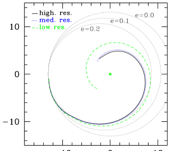
Figure 1: A depiction of the orbit for the simulation described in the text (see also Table 1). The figure shows the coordinate position of the center of one apparent horizon relative to the other, in the orbital plane $z=0$. The units have been scaled to the mass $M_{0}$ of a single black hole, and curves are shown from simulations with three different resolutions. Overlaid on this figure are reference ellipses of eccentricity $0$, $0.1$ and $0.2$, suggesting that if one were to attribute an initial eccentricity to the orbit it could be in the range $0-0.2$.

		low res.	med. res.	high res.
	ADM Mass	$2.36M_{0}$	$2.39M_{0}$	$2.39M_{0}$
initial	BH masses	$0.97M_{0}$	$0.99M_{0}$	$M_{0}$
	orbital eccentricity	$0-0.2$	$0-0.2$	$0-0.2$
	proper separation	$16.5M_{0}$	$16.6M_{0}$	$16.6M_{0}$
	angular velocity $\times M_{0}$	$0.023$	$0.023$	$0.023$
final	BH mass	$1.77M_{0}$	$1.85M_{0}$	$1.90M_{0}$
	BH spin parameter	$0.74$	$0.73$	$0.70$

Table 1: Some properties of the simulated equal mass binary system described in the text. Where relevant the units have been scaled to the mass $M_{0}$ of one of the initial black holes, measured from the higher resolution simulation at a time after the majority of scalar field accretion has occurred. The final black hole mass and spin where estimated from data as shown in Fig. 2, a little while after the black hole formed, though not so long after as to be affected by the “drift” from numerical error. The initial proper separation was measured at $t=10M_{0}$, and is the proper length of the piece of a coordinate line outside the apparent horizons that connects their coordinate centers. The black holes initially have zero spin.

Fig. 2 shows the horizon masses and final horizon angular momentum as a function of time. The ADM mass of the space time suggests that approximately $15\%$ of the total scalar field energy does not collapse into black holes. The remnant scalar field leaves the vicinity of the orbit quite rapidly (in $t\approx 30M_{0}$, which is on the order of the light crossing time of the orbit). Black hole masses are estimated from the horizon area $A$ and angular momentum $J$, and applying the Smarr formula:

$$M=\sqrt{M_{ir}^{2}+J^{2}/(4M_{ir}^{2})},\ \ \ M_{ir}\equiv\sqrt{A/16\pi}.$$ (4)

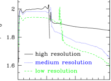
Figure 2: The plot to the left shows the net black hole mass of the spacetime in units of the mass $M_{0}$ of a single initial black hole, calculated from apparent horizon (AH) properties (using (4) with the dynamical horizon estimate for $J$), and from simulations with three different resolutions. The initial sharp increase in mass is due to scalar field accretion, the small “wiggle” at around $20M_{0}$ appears to be a gauge effect, and the “jaggedness” around the time of the merger is due to robustness problems in the AH finder that manifest when the AH shapes are highly distorted. To the right the Kerr parameter $a$ of the final black hole is shown (for clarity we only plot the results from a single simulation), calculated using the ratio $C_{r}$ of polar to equatorial proper circumference of the AH and applying (5), and using the dynamical horizon framework (curve labeled DH). The loss of mass (and similarly increase in $a$) with time after the merger is due to accumulating numerical error.

The horizon angular momentum of the final black hole is calculated using two methods (which do give zero angular momentum when applied to the initial black holes, as expected). First, by using the dynamical horizon frameworkashtekar_krishnan , though assuming that the rotation axis of the black hole is orthogonal to the $z=0$ orbital plane, and that each closed orbit of the azimuthal vector field (which at late times should become a Killing vector) lies in a $z={\rm constant}$ surface of the simulation. Due to the symmetry of the initial data, these assumptions are probably valid, though this will eventually need to be confirmed. The second method, following brandt_seidel , is to measure the ratio $C_{r}$ of the polar to equatorial proper radius of the horizon, and use the formula that closely approximates the function that is valid for Kerr black holes:

$$a\approx\sqrt{1-\left(2.55C_{r}-1.55\right)^{2}}$$ (5)

As seen in Fig. 2, the initial ringing of the black hole is quite apparent in the estimate using $C_{r}$. Remarkably, the dynamical horizon estimate for $a$ and average value obtained using $C_{r}$ agree quite closely, even shortly after the merger when one might have expected the black hole to still be too far from its stationary state to have either method be applicable.

To estimate the gravitational waves emitted by the binary we use the Newman-Penrose scalar $\Psi_{4}$, with the null tetrad constructed from the unit timelike normal $n^{\mu}$, a radial unit spacelike vector normal to $r={\rm constant}$ coordinate spheres, and two additional unit spacelike vectors orthogonal to the radial vector. Far from the source, the real and imaginary components of $\Psi_{4}$ are proportional to the second time derivatives of the two polarizations of the emitted gravitational wave. Fig. 3 shows an example of the real part of $\Psi_{4}$. Most of the early, short wavelength burst of waves can be correlated with the passage of the remnant scalar field that did not fall into the black holes (the “noisy” nature of this piece of the waveform is in part due to numerical error). This unwanted radiations leaves the domain quite early on, and so does not significantly affect the subsequent merger waves. Roughly the first long wavelength oscillation in the plot can be associated with orbital motion, and subsequent waves with the ringdown of the final black hole.

Figure 3: A sample of the gravitational waves emitted during the merger, as estimated by the Newman-Penrose scalar $\Psi_{4}$ (from the medium resolution simulation). Here, the real component of $\Psi_{4}$ multiplied by the coordinate distance $r$ from the center of the grid is shown at a fixed angular location, though several distances $r$. The waveform has also been shifted in time by amounts shown in the plot, so that the oscillations overlap. If the waves are measured far enough from the central black hole then the amplitudes should match, and they should be shifted by the light travel time between the locations (i.e. by $25M_{0}$ in this example). That we need to shift the waveforms by more than this suggests the extraction points are still too close to the black hole; the decrease in amplitude is primarily due to numerical error as the wave moves into regions of the grid with relatively low resolution.

To estimate the total energy $E$ emitted in gravitational waves, we use the following formula smarr_rad

$$\frac{dE}{dt}=\frac{R^{2}}{4\pi}\int pd\Omega,\ \ \ p=\int_{0}^{t}\Psi_{4}dt\cdot\int_{0}^{t}\bar{\Psi}_{4}dt,$$ (6)

where $\bar{\Psi}_{4}$ is the complex conjugate of $\Psi_{4}$, and the surface integrated over in (6) is a sphere of constant coordinate radius $R$ (in uncompactified coordinates). This method of calculating the energy is quite susceptible to numerical error, as we are summing a positive definite quantity over all time to give a change of energy with respect to time; thus numerical error in $\Psi_{4}$ will tend to inflate the answer. To reduce some of this error, we filter out the high spherical harmonic components ($\geq\ell=|m|=6$) of $\Psi_{4}$ before applying (6). Note that the smaller integration radii (as shown in Fig. 3) are not very far from the binary system, and so possibly in a region where (6) is not strictly valid. However, the larger integration radii are in regions of the grid that do not have very good resolution (due both to the mesh refinement structure and the spatially compactified coordinate domain), and so numerical error (mostly dissipation) tends to reduce the amplitude of the waves with distance from the source. With all these caveats in mind, the numbers we obtain from (6) are $4.7\%,3.2\%,2.7\%,2.3\%$ at integration radii of $25M_{0},50M_{0},75M_{0}$ and $100M_{0}$ respectively (from the high resolution simulation), and where the percentage is relative to $2M_{0}$. Another estimate of the radiated energy can be obtained by taking the difference between the final and initial horizon masses (Table 1)—this suggests around $5\%$ (high resolution case).

V. Conclusion: In this letter we have described a numerical method based on generalized harmonic coordinates that can stably evolve (at least a class of) binary black hole spacetimes. As an example, we presented an evolution of a binary system composed of non-spinning black holes of equal mass $M_{0}$, with an initial proper separation and orbital angular velocity of approximately $16.6M_{0}$ and $0.023/M_{0}$ respectively. The binary merged within approximately 1 orbit, leaving behind a blackhole of mass $M_{f}\approx 1.9M_{0}$ and angular momentum $J\approx 0.70M_{f}^{2}$. A calculation of the energy emitted in gravitational waves indicates that roughly $5\%$ of the initial mass (defined as $2M_{0}$) is radiated . Future work includes improving the accuracy of simulation (in particular the gravitational waves), exploring a larger class of initial conditions (binaries that are further separated, have different initial masses, non-zero spins, etc.), and attempting to extract more geometric information about the nature of the merger event from the simulations.

Acknowledgments: I would like to thank Carsten Gundlach for describing their constraint damping method for the Z4 systemgundlach_et_al , and suggesting that it can be applied in a similar fashion with the harmonic scheme. I would also like to thank Matthew Choptuik, Luis Lehner and Lee Lindblom for stimulating discussions related to this work. I gratefully acknowledge research support from NSF PHY-0099568, NSF PHY-0244906 and Caltech’s Richard Chase Tolman Fund. Simulations were performed on UBC’s vn cluster, (supported by CFI and BCKDF), and the Westgrid cluster (supported by CFI, ASRI and BCKDF).

References

- (1) L. Blanchet, Living Rev.Rel. 5, 3 (2002)
- (2) R. Price and J. Pullin, Phys. Rev. Lett. 72, 3297 (1994)
- (3) L. Smarr, Ph.D. thesis, University of Texas, Austin, 1975.
- (4) B. Bruegmann, Int.J.Mod.Phys. D8 85, (1999)
- (5) S. Brandt et al., Phys.Rev.Lett. 85 5496, (2000)
- (6) J. Baker, B. Bruegmann, M. Campanelli, C. O. Lousto and R. Takahashi Phys.Rev.Lett. 87 121103, (2001)
- (7) B. Bruegmann, W. Tichy and N. Jansen Phys.Rev.Lett. 92 211101, (2004)
- (8) M. Alcubierre et al., gr-qc/0411149 (2004)
- (9) F. Pretorius, Class. Quant. Grav. 22 425, (2005)
- (10) D. Garfinkle, Phys.Rev. D65, 044029 (2002)
- (11) B. Szilagyi and J. Winicour, Phys.Rev. D68, 041501 (2003)
- (12) O. Brodbeck, S. Frittelli, P. Huebner and O. A. Reula, J.Math.Phys. 40, 909 (1999)
- (13) C. Gundlach, J.M. Martin-Garcia, G. Calabrese and I. Hinder, gr-qc/0504114 (2005)
- (14) G. B. Cook, Living Rev.Rel. 3, 5 (2000)
- (15) A. Ashtekar and B. Krishnan Living Rev.Rel. 7, 10 (2004)
- (16) S.R. Brandt and E. Seidel, Phys.Rev. D52, 870 (1995)
- (17) L. Smarr, in Sources of Gravitational Radiation, ed. L. Smarr, Seattle, Cambridge University Press (1978)