An aligned-spin neutron-star–black-hole waveform model based on the effective-one-body approach and numerical-relativity simulations

Abstract

After the discovery of gravitational waves from binary black holes (BBHs) and binary neutron stars (BNSs) with the LIGO and Virgo detectors, neutron-star–black-holes (NSBHs) are the natural next class of binary systems to be observed. In this work, we develop a waveform model for aligned-spin neutron-star–black-holes (NSBHs) combining a BBH baseline waveform (available in the effective-one-body approach) with a phenomenological description of tidal effects (extracted from numerical-relativity simulations), and correcting the amplitude during the late inspiral, merger and ringdown to account for the NS tidal disruption. In particular, we calibrate the amplitude corrections using NSBH waveforms obtained with the numerical-relativity spectral Einstein code (SpEC) and the SACRA code. The model was calibrated using simulations with NS masses in the range $1.2-1.4M_{\odot}$, tidal deformabilities up to $4200$ (for a 1.2 $M_{\odot}$ NS), and dimensionless BH spin magnitude up to 0.9. Based on the simulations used, and on checking that sensible waveforms are produced, we recommend our model to be employed with NS mass in the range $1\mbox{--}3M_{\odot}$, tidal deformability $0\mbox{--}5000$, and (dimensionless) BH spin magnitude up to $0.9$. We also validate our model against two new, highly accurate NSBH waveforms with BH spin 0.9 and mass ratios 3 and 4, characterized by tidal disruption, produced with SpEC, and find very good agreement. Furthermore, we compute the unfaithfulness between waveforms from NSBH, BBH, and BNS systems, finding that it will be challenging for the advanced LIGO-Virgo–detector network at design sensitivity to distinguish different source classes. We perform a Bayesian parameter-estimation analysis on a synthetic numerical-relativity signal in zero noise to study parameter biases. Finally, we reanalyze GW170817, with the hypothesis that it is a NSBH. We do not find evidence to distinguish the BNS and NSBH hypotheses, however the posterior for the mass ratio is shifted to less equal masses under the NSBH hypothesis.

I Introduction

In their first two observing runs (O1 and O2), Advanced LIGO Aasi et al. (2015) and Advanced Virgo Acernese et al. (2015) have observed gravitational waves (GWs) from ten binary black holes (BBHs) and one binary neutron star (BNS), GW170817 Abbott et al. (2019a). Recently, in the third observing run (O3), a second BNS, GW190425, was discovered Abbott et al. (2020a). Other groups have reported additional GW observations analyzing the public data from the first two runs Venumadhav et al. (2019); Zackay et al. (2019a, b). Neutron-star–black-holes (NSBHs) may be the next source class to be discovered. Given the lack of a detection in O1 and O2, the rate of NSBHs is uncertain. However, based on estimates from Ref. Abadie et al. (2010), the expected number of NSBH detections is $0_{-0}^{+19}$ O3 and $1_{-1}^{+91}$ in O4 Abbott et al. (2018a), where the central value is the median and the error bars give the 90% credible interval. As of this writing, in O3, the LIGO and Virgo Collaborations have published seven circulars via the Gamma-ray Coordinates Network (GCN) describing detection candidates for which the probability of the system being a NSBH is larger than 1%, and for which the candidate has not been retracted LIGO Scientific Collaboration, Virgo Collaboration (2019a, b, c, d, e, f, 2020). Furthermore, GW data alone does not exclude the possibility that GW170817 is a NSBH Hinderer et al. (2019); Coughlin and Dietrich (2019); Abbott et al. (2020b), and it has also been suggested that GW190425 could be a NSBH Han et al. (2020); Kyutoku et al. (2020). Therefore it is timely to develop methods that can be used to study NSBHs in GW data.

NSBH binaries exhibit a rich phenomenology that is imprinted on the gravitational waveform (for a review see Ref. Shibata and Taniguchi (2011)). First, as is the case for BNS systems, finite size effects cause a dephasing of the waveform relative to a BBH with the same masses and spins Flanagan (1998); Flanagan and Hinderer (2008); Vines and Flanagan (2013); Pannarale et al. (2011a). Additionally, the amplitude of NSBH waveforms can be affected by tidal forces Kyutoku et al. (2010). For unequal mass ratios and slowly spinning BHs, the amplitude of the waveform is well-described by a BBH Foucart et al. (2013a). On the other hand, for near-equal mass ratios or for highly spinning BHs, depending on the NS equation of state (EOS), the NS can undergo tidal disruption, in which the star is ripped apart as it approaches the BH Foucart et al. (2011); Kyutoku et al. (2010, 2011); Foucart et al. (2013b); Kawaguchi et al. (2015). If the disruption takes place before the NS crosses the innermost stable circular orbit, then the material ejected from the NS can form a disk around the BH Pannarale et al. (2011b); Foucart (2012); Lovelace et al. (2013). If so, starting at a characteristic (cutoff) frequency Kyutoku et al. (2010); Kawaguchi et al. (2017); Pannarale et al. (2015a), the amplitude of the waveform is strongly suppressed, and the ringdown stage is reduced or even effaced. The details of this process contain information about the NS EOS. Additionally, NSBH mergers can be the progenitors of short gamma-ray bursts Paczynski (1986); Eichler et al. (1989); Paczynski (1991); Meszaros and Rees (1992); Narayan et al. (1992); Nakar (2007), and the disk around the remnant BH and dynamical ejecta can provide the engine for the kilonova signal Metzger (2017); Tanaka (2016), like the ones observed for GW170817 Abbott et al. (2019a); Abbott et al. (2017a).

In order to take advantage of this potentially rich source of information, it is crucial to have a fast and accurate waveform model capturing effects due to relativistic matter, which can be used in analyzing GW data. Several approaches exist for describing finite-size effects in BNS systems. Tidal corrections Flanagan (1998); Flanagan and Hinderer (2008); Vines and Flanagan (2013); Damour and Nagar (2009); Binnington and Poisson (2009a) have been incorporated in the effective one-body (EOB) formalism Buonanno and Damour (1999, 2000); Damour et al. (2000) in Refs. Damour and Nagar (2010); Damour et al. (2012); Steinhoff et al. (2016); Hinderer et al. (2016); Nagar et al. (2018); Lackey et al. (2019). References Dietrich et al. (2017); Dietrich et al. (2019a) developed a flexible technique that starts from a point-mass BBH baseline waveform, and applies tidal-phase modifications by fitting a Padé-resummed post-Newtonian (PN)–based ansatz to the phasing extracted from numerical-relativity (NR) simulations (henceforth, we refer to this as the NRTidal approach). These corrections have been applied to BBH baselines produced within the EOBNR framework Bohé et al. (2017), and within the inspiral-merger-ringdown phenomenological (IMRPhenom) approach Khan et al. (2016); Hannam et al. (2014).

Name in this paper	LAL name	Ref.
SEOBNR_BBH	SEOBNRv4_ROM	Bohé et al. (2017)
SEOBNR_BNS	SEOBNRv4_ROM_NRTidalv2	Dietrich et al. (2019a)
SEOBNR_NSBH	SEOBNRv4_ROM_NRTidalv2_NSBH	this paper

Table 1: Dictionary relating the names we use in this paper for several waveforms from the SEOBNR family and the corresponding names of the waveforms implemented in the LIGO Algorithms Library (LAL). The second and third waveforms use tidal effects within the NRTidal approach.

There have been several previous works constructing NSBH waveforms. An aligned-spin NSBH waveform model was developed in Refs. Lackey et al. (2012, 2014), but it covered a limited range of mass ratios. In Ref. Kumar et al. (2017), this waveform model was used in parameter and population studies in conjunction with a former version of the EOBNR BBH baseline Taracchini et al. (2014). A NSBH model called PhenomNSBH, which was constructed using a similar approach to modeling NSBHs as the one discussed in this paper but developed within the IMRPhenom approach, was recently put forward in Ref. Thompson et al. (2020). This model uses the method of Ref. Pannarale et al. (2015b) to describe tidal disruption of the amplitude, and uses the tidal phase corrections from Ref. Dietrich et al. (2019a).

In this work we develop a frequency-domain model for the dominant, quadrupolar multipole of GWs emitted by aligned-spin NSBH systems. Together with the recent waveform model of Ref. Thompson et al. (2020), these are the first NSBH models covering a wide range of mass ratios and spin that can be used to analyze GW data. In this paper, we refer to our model as SEOBNR_NSBH, which has already been implemented in the LIGO Algorithms Library (LAL) The LIGO Scientific Collaboration (2020). In Table 1 we provide a dictionary between the names we use in this work, and the name as implemented in LAL. The amplitude is based on an EOBNR BBH baseline model that we refer to as SEOBNR_BBH Bohé et al. (2017). We apply corrections inspired by Pannarale et al. Pannarale et al. (2015b) to account for tidal disruption. We have adapted the corrections of Ref. Pannarale et al. (2015b), originally developed for a former version of the IMRPhenom BBH model Santamaria et al. (2010), for use with EOBNR waveforms Bohé et al. (2017), augmented with reduced-order modeling (ROM) Pürrer (2014, 2016) to enhance the speed. Differently from Ref. Thompson et al. (2020), which uses the fit from Pannarale et al. Pannarale et al. (2015b), here we have performed a fit incorporating results from the new NSBH simulations at our disposal as described in Sec. II.2. While the publicly available SXS simulations were not used for calibration of Ref. Thompson et al. (2020), these waveforms were used for validation and good agreement was found. The phase is computed by applying tidal corrections to the EOBNR BBH baseline Bohé et al. (2017) using the NRTidal approach, as in SEOBNR_BNS Dietrich et al. (2019a). As shown in Ref. Foucart et al. (2019a), even though the tidal corrections from SEOBNR_BNS were derived from BNS simulations, they give good agreement with NSBH simulations.

The rest of this paper is organized as follows. In Sec. II, we describe the construction of the waveform model. We review properties of NSBH systems in Sec. II.1, summarize the NR waveforms that we use in Sec. II.2, give an outline of the waveform model in Sec. II.3, summarize the procedure used to calibrate the amplitude correction, assess their accuracy by computing the unfaithfulness, and compare the NSBH waveforms to NR simulations in Sec. II.4. Then, we discuss the regime of validity in Sec. II.5. Next, we apply the waveform model to several data analysis problems. First, in Sec. III.1 we estimate when the advanced LIGO-Virgo detector network at design sensitivity can distinguish NSBH and BBH, and NSBH and BNS, systems. Then, in Sec. III.2 we perform parameter-estimation Bayesian analysis on an NR-waveform, hybridized to an analytical waveform at low frequency, and show the differences between recovering this waveform with a BBH and NSBH model. Finally, we reanalyze GW170817 under the hypothesis that it is a NSBH in Sec. III.3. We conclude in Sec. IV by summarizing the main points and lay out directions for future improvements. Finally, in Appendix A, we give explicit expressions defining the waveform model.

We work in units with $G=c=1$. The symbol $M_{\odot}$ refers to the mass of the sun.

II Constructing the NSBH waveform model

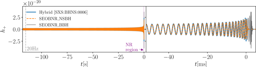
Figure 1: We compare an NR-hybrid waveform, which is constructed by stitching together the SXS:BHNS:0006 ($M_{\rm NS}=1.4M_{\odot}$, $M_{\rm BH}=2.1M_{\odot}$, $\Lambda_{\rm NS}=791$) and SEOBNR_BNS ($m_{1}=1.4M_{\odot}$, $m_{2}=2.1M_{\odot}$, $\Lambda_{1}=0$, $\Lambda_{2}=791$) waveforms, with the SEOBNR_NSBH ($M_{\rm NS}=1.4M_{\odot}$, $M_{\rm BH}=2.1M_{\odot}$, $\Lambda_{\rm NS}=791$) and SEOBNR_BBH ($m_{1}=1.4M_{\odot}$, $m_{2}=2.1M_{\odot}$, $\Lambda_{1}=\Lambda_{2}=0$) waveforms. The strain is produced by a source at a distance of 1 Mpc. The definition of the tidal parameter $\Lambda_{\rm NS}$ is given in Eq. 4. In the left panel, we show the waveforms during the long inspiral and mark $20\,{\rm Hz}$, which is the lower frequency typically used for LIGO-Virgo parameter-estimation analyses. We also indicate the region toward merger where the NR data are available. In the right panel, we zoom into the last stages of the inspiral and merger. Due to tides, the hybrid waveform and SEOBNR_NSBH have a faster inspiral, and end earlier than the corresponding point-mass SEOBNR_BBH waveform. Furthermore, because of tidal disruption, the hybrid and SEOBNR_NSBH waveforms have no ringdown phase, but end abruptly when the NS gets disrupted. Overall, we find very good agreement between SEOBNR_NSBH and NR-hybrid waveforms throughout the entire coalescence.

II.1 NSBH binary properties

We begin by providing a brief description of the final stages of a NSBH coalescence, identifying the main features of the process and the physical properties of the remnant BH. Here, we mainly follow the discussion in Refs. Shibata and Taniguchi (2011); Foucart (2012); Pannarale et al. (2015b).

The two bodies spiral in due to the loss of energy from the emission of GWs. If the NS approaches close enough to the BH, tidal forces exerted by the BH on the NS can overcome the self gravity of the NS, causing the star to loose mass. This process is called mass shedding. This in turn often leads to tidal disruption, in which the NS is completely torn apart by the strong gravitational field of the BH. Let us denote with $r_{\rm tide}$ the separation of the binary at which mass shedding begins. To understand the fate of the NS and the characteristics of the GW signal emitted during the last stages of inspiral, plunge and merger, we compare $r_{\rm tide}$ to the location of the innermost-stable circular orbit (ISCO) (which marks the beginning of the plunge). If $r_{\rm tide}<r_{\rm ISCO}$, the NS is swallowed by the BH, without loss of material. By contrast, if $r_{\rm tide}>r_{\rm ISCO}$, mass is ejected from the NS before it plunges. If the NS is far away from the ISCO when it is disrupted, matter may form an accretion disk (torus) around the BH after merger. It has been shown (e.g., see Refs Kyutoku et al. (2010, 2011); Foucart (2012); Lovelace et al. (2013) and also below) that the disruption affects the GW signal for NSBH binaries with either nearly equal masses or large BH spins aligned with the orbital angular momentum, because for those systems the condition $r_{\rm tide}<r_{\rm ISCO}$ is satisfied. In Fig. 1, we show an illustration of the effect of tidal disruption on the GW waveform for an example NR hybrid with mass ratio 1.5.

Let us now estimate the radial separation at which mass shedding occurs, $r_{\rm tide}$, by imposing that the tidal force from the BH balances the self-gravity of the NS. As described in Ref. Foucart (2012), in the Newtonian limit, $r_{\rm tide}$ can be estimated as $r_{\rm tide}\approx\xi_{\rm Newt}R_{\rm NS}$, where $\xi_{\rm Newt}=(3Q)^{1/3}$, $R_{\rm NS}$ is the NS radius in isolation, $Q\equiv M_{\rm BH}/M_{\rm NS}$ is the mass ratio, $M_{\rm BH}$ is the mass of the BH, and $M_{\rm NS}$ is the mass of the NS. The factor of 3 is an estimate obtained by matching with NR simulations. This estimate can be improved by accounting for relativistic effects due to the large compactness of the NS, $C_{\rm NS}\equiv M_{\rm NS}/R_{\rm NS}$ Foucart (2012). First, $r_{\rm tide}$ is reduced by a factor $(1-2C_{\rm NS})$ relative to the Newtonian estimate; this factor enforces the absence of tidal disruption in the BH limit $C_{\rm NS}\rightarrow 1/2$. Second, point-mass motion in the Kerr metric leads to a correction factor $\xi$ which differs from the Newtonian estimate Foucart (2012); Fishbone (1973). Combining these effects, we have

$$r_{\rm tide}=\xi(1-2C_{\rm NS})R_{\rm NS}\,.$$ (1)

The relativistic correction parameter $\xi$ is determined by solving the algebraic equation (we take the largest positive root of this equation)

$$\left(\frac{\xi}{\xi_{\rm Newt}}\right)^{3}=\frac{\xi^{2}-2QC_{\rm NS}\xi+Q^{2}C_{\rm NS}^{2}\chi_{\rm BH}^{2}}{\xi^{2}-3QC_{\rm NS}\xi+2\chi_{\rm BH}\sqrt{Q^{3}C_{\rm NS}^{3}\xi}},$$ (2)

where $\chi_{\rm BH}$ is the spin of the BH. We can associate to the tidal-disruption separation a frequency, which is more useful in the context of modeling the gravitational waveform, as follows

$$f_{\rm tide}=\frac{1}{\pi(\chi_{\rm BH}M_{\rm BH}+\sqrt{r_{\rm tide}^{3}/M_{\rm BH}})},$$ (3)

which is obtained from the (circular orbit) relation between radial separation and (angular) orbital frequency in the Kerr geometry.

The NS compactness $C_{\rm NS}$, which depends on the NS EOS, enters the expression for $r_{\rm tide}$. In order to avoid making an assumption about the EOS, it is more convenient to work in terms of the dimensionless tidal-deformability parameter $\Lambda_{\rm NS}$, which relates the quadrupole moment of the NS to the tidal field of the companion. The tidal parameter is determined by the compactness of the NS and the tidal Love number $k_{2}$ as follows

$$\Lambda_{\rm NS}=\frac{2}{3}\frac{k_{2}}{C_{\mathrm{NS}}^{5}}.$$ (4)

We take the tidal parameter of the BH to be zero. The tidal parameter of non-spinning BHs was shown to be zero in Ref. Binnington and Poisson (2009b) f. We can relate $\Lambda_{\rm NS}$ and $C_{\rm NS}$ in an equation-of-state independent way with the $\Lambda_{\rm NS}-C_{\rm NS}$ relation Yagi and Yunes (2017)

$$C_{\rm NS}=\sum_{k=0}^{2}a_{k}(\ln\Lambda_{\rm NS})^{k},$$ (5)

with $a_{0}=0.360,a_{1}=-0.0355,a_{2}=0.000705$. In order to achieve continuity with BBH waveforms in the limit $\Lambda_{\rm NS}\rightarrow 0$, for $\Lambda_{\rm NS}\leq 1$, we replace the $\Lambda_{\rm NS}-C$ relation with a cubic polynomial which interpolates from $\Lambda_{\rm NS}=1$ to $C_{\rm NS}=1/2$ at $\Lambda_{\rm NS}=0$, and it is continuous and once differentiable at $\Lambda_{\rm NS}=1$. The universal relations are also used in Ref. Thompson et al. (2020).

The matter ejected from the NS, during tidal disruption, can remain bound, forming a disk (torus) around the remnant BH. The mass of this remnant torus, $M_{\rm{b,torus}}$, can be determined in terms of the baryonic mass of the NS using fits from Ref. Foucart (2012) (see also more recent simulations performed in Ref. Foucart et al. (2019b))

$$\frac{M_{\rm b,torus}}{M_{\rm b,NS}}={\rm max}\left(\frac{0.296r_{\rm tide}-0.171r_{\rm ISCO}}{R_{\rm NS}},0\right),$$ (6)

where the ISCO radius ($r_{\rm ISCO}$) in the Kerr spacetime is given by

$$r_{\rm ISCO} = 3+Z_{2}\mp\sqrt{(3-Z_{1})(3+Z_{1}+2Z_{2})}\,,$$ (7a)

$$Z_{1} = 1+(1-\chi_{\rm BH}^{2})^{1/3}\left[(1+\chi_{\rm BH})^{1/3}+\right.$$ (7b)

$$\left.(1-\chi_{\rm BH})^{1/3}\right]\,,$$

$$Z_{2} = \sqrt{3\chi_{\rm BH}^{2}+Z_{1}^{2}},$$ (7c)

where the $\mp$ sign holds for prograde (retrograde) orbits.

As mentioned above, the onset of mass shedding occurs when the objects approach within a distance $r_{\rm tide}$ before the NS cross the ISCO. However, the ISCO does not introduce a definite feature in the gravitational waveform. In order to identify the onset of tidal disruption with a definite feature in an NR waveform, in our model we compare $f_{\rm tide}$ to the ringdown frequency of the final BH, $f_{\rm RD}$, which is the frequency of least-damped quasinormal mode of the final BH. The ringdown frequency can be computed from the final mass and spin using fitting formulas from Ref. Berti et al. (2006). To obtain the final mass and spin from the initial parameters of the binary, we use the fits performed by Ref. Zappa et al. (2019), which account for the ejected mass.

II.2 Numerical-relativity waveforms

In this section we briefly describe the NR data used to construct and validate the model. The Simulating eXtreme Spacetimes (SXS) collaboration has publicly released data from seven simulations described in Refs. Foucart et al. (2013c); Foucart et al. (2019a), which were produced using the Spectral Einstein Code (SpEC), see Ref. SPE (2018). The hyrodynamical part of the code is described in Ref. Duez et al. (2008); Foucart et al. (2013d). These configurations do not contain spinning BHs, but do include mergers with and without tidal disruption. These simulations use an ideal gas EOS with polytropic index $\Gamma=2$, except for the mass ratio 3 simulation SXS:BHNS:0003, which uses a piecewise polytropic ansatz calibrated to the H1 EOS, see Ref. Read et al. (2009). We refer the reader to Ref. Foucart et al. (2019a) for further explanation. For five of these simulations the NS spin is zero, and we use these simulations to fit the model as described in Sec. II.4. We use the other two simulations for verification. Additionally, SpEC has simulated nine systems with large BH spin in Ref. Foucart et al. (2014), using the more advanced temperature and composition dependent LS220 EOS Lattimer and Swesty (1991), which we also use to fit our waveform model. Finally, we validate our NSBH model also against two new SXS waveforms, Q3S9 and Q4S9, which are highly accurate simulations describing disruptive mergers with large BH spin. These simulations were also performed using the $\Gamma=2$ EOS. We give the parameters of all SXS waveforms used here in Table LABEL:tab:SXS-spinning-BH.

In fitting the model, we also use 134 simulations of irrotational NSs performed with the SACRA code Yamamoto et al. (2008), which were presented in Refs. Kyutoku et al. (2010, 2011). These simulations span the mass ratios $Q=\{2,3,4,5\}$, BH spins $\chi_{\rm BH}=\{-0.5,0,0.25,0.5,0.75\}$, and a range of piecewise polytropic EOS. The parameters for all of the waveforms and the EOS used are given Table II of Ref. Lackey et al. (2014). Whereas the large number of SACRA waveforms lets us probe a wide parameter range, these waveforms are shorter and of lower accuracy than the publicly available SpEC waveforms as well as Q3S9 and Q4S9, due to finite numerical resolution and non-negligible eccentricity in the initial data. We note that these simulations predate the public SXS simulations by a number of years.

Label	$\frac{M_{\rm BH}}{M_{\odot}}$	$\frac{M_{\rm NS}}{M_{\odot}}$	$Q$	$\chi_{\rm BH}$	$\chi_{\rm NS}$	$\Lambda_{\rm NS}$	$N_{\rm GW}$	$e_{\rm res}$
SXS:BHNS:0001	8.4	1.4	6	0	0	526	25.3	$<1.3\times 10^{-3}$
SXS:BHNS:0002	2.8	1.4	2	0	0	791	26.1	$<5\times 10^{-4}$
SXS:BHNS:0003	4.05	1.35	3	0	0	624	12.3	$7.9\times 10^{-3}$
SXS:BHNS:0004	1.4	1.4	1	0	0	791	24.5	$<6.0\times 10^{-5}$
SXS:BHNS:0006	2.1	1.4	1.5	0	0	791	33.2	$<2.7\times 10^{-4}$
M12-7-S8-LS220	7	1.2	5.8	0.8	0	1439	17.8	$2.7\times 10^{-2}$
M12-7-S9-LS220	7	1.2	5.8	0.9	0	1439	18.9	$2.6\times 10^{-2}$
M12-10-S8-LS220	10	1.2	8.3	0.8	0	1439	20.3	$3.1\times 10^{-2}$
M12-10-S9-LS220	10	1.2	8.3	0.9	0	1439	22.1	$3.3\times 10^{-2}$
M14-7-S7-LS220	7	1.4	5	0.7	0	536	10.6	$3.9\times 10^{-2}$
M14-7-S8-LS220	7	1.4	5	0.8	0	536	11.7	$3.7\times 10^{-2}$
M14-7-S9-LS220	7	1.4	5	0.9	0	536	12.5	$3.7\times 10^{-2}$
M14-10-S8-LS220	10	1.4	7.1	0.8	0	536	15.1	$4.2\times 10^{-2}$
M14-10-S9-LS220	10	1.4	7.1	0.9	0	536	16.8	$4.3\times 10^{-2}$
SXS:BHNS:0005	1.4	1.4	1	0	-0.2	791	21.6	$5.0\times 10^{-4}$
SXS:BHNS:0007	2.8	1.4	2	0	-0.2	791	24.7	$<4.7\times 10^{-4}$
Q3S9	4.2	1.4	3	0.9	0	791	26.5	$5.4\times 10^{-4}$
Q4S9	5.6	1.4	4	0.9	0	791	31.4	$1.7\times 10^{-3}$

Table 2: Parameters for the SXS NSBH waveforms used in this work. The simulations above the horizontal line were used to fit the NSBH model, the simulations below the line are used for validation. Parameters for the other waveforms that we employ to fit the model were produced by the SACRA code, and are given in Table II of Ref. Lackey et al. (2014). We also report the number of GW cycles, $N_{\rm GW}$, computed up to the peak of the dominant GW mode. Finally we display the residual eccentricity, $e_{\rm res}$.

II.3 Parameterization of the NSBH waveform model

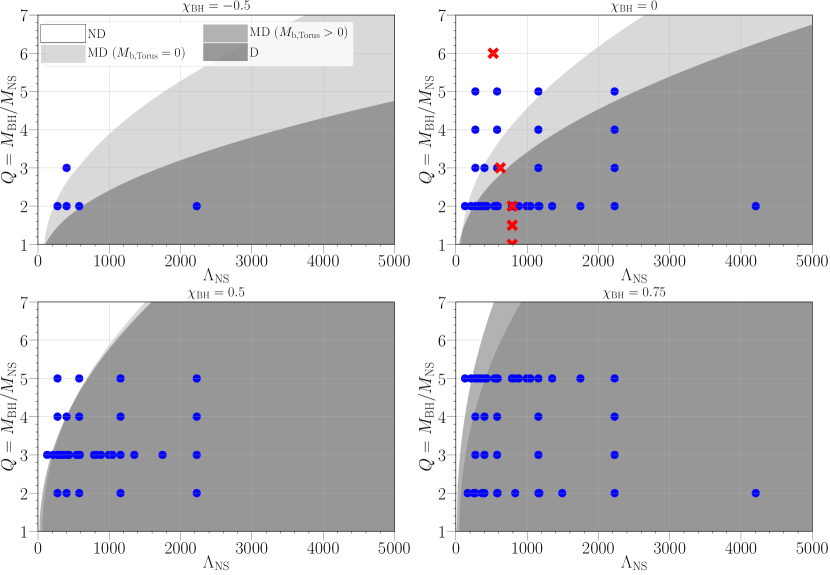
Figure 2: Representative parameter space region in the $Q-\Lambda_{\rm NS}$ plane for different values of the BH spin $\chi_{\rm BH}$. We show the regions for the different classes of NSBHs, using the model described in the main text: white regions represent non-disruptive mergers (ND), light gray regions represent mildly disruptive mergers without a torus remnant (MD, $M_{\rm b,torus}\neq 0$), the medium gray shade visible in the $\chi_{\rm BH}=0.75$ figure represents mildly disruptive mergers with a torus remnant (MD, $M_{\rm b,torus}=0$), and the dark gray region marks disruptive mergers with a torus remnant (D). We also mark the parameter values of (some of) the NR simulations used. Dots (crosses) represent simulations produced by the SACRA (SpEC) code. Not shown are 12 SACRA waveforms with $\chi_{\rm BH}=0.25$, two SpEC waveforms with NS spin different from zero, and eleven SpEC waveforms with $\chi_{\rm BH}=\{0.7,0.8,0.9\}$.

We limit the waveform modeling to the dominant quadrupolar multipole, notably the modes $\ell=2,m=\pm 2$ in the -2 spin-weighted spherical harmonic decomposition of the gravitational polarizations $h_{+,\times}$, and to aligned-spin NSBHs. In the frequency domain, we can write the waveform as

$$h(f)=A(f)e^{i\phi(f)}.$$ (8)

Henceforth, we focus on the dependence of the amplitude $A(f)$ and phase $\phi(f)$ on the intrinsic parameters of the binary, $\vec{\theta}=\{M_{\rm BH},M_{\rm NS},\chi_{\rm BH},\chi_{\rm NS},\Lambda_{\rm NS}\}$, where we indicate with $\chi_{\rm BH}$ and $\chi_{\rm NS}$ the (dimensionless) components of the spin aligned with the orbital angular momentum, for the BH and NS, respectively.

To compute the GW phase $\phi(f)$, we use the point-mass baseline SEOBNR_BBH model, and apply tidal corrections from the NRTidal framework, as in Ref. Dietrich et al. (2019a). As shown in Ref. Foucart et al. (2019a) (and as we verify in Figs. 5 and 6), applying NRTidal corrections gives a reasonable approximation of the phase, until the last few cycles.

In order to model the amplitude $A(f)$, we start with the BNS model SEOBNR_BNS as a baseline. Since this model includes tapering beyond the BNS merger frequency Dietrich et al. (2019b), we first remove this tapering. This is necessary since the tapering depends on the tidal parameters of both objects, $\Lambda_{1}$ and $\Lambda_{2}$, and does not vanish as $\Lambda_{1}\rightarrow 0$. We note that this means that the $\Lambda_{1}\rightarrow 0$ limit of SEOBNR_BNS does not correctly describe the amplitude of a NSBH system.

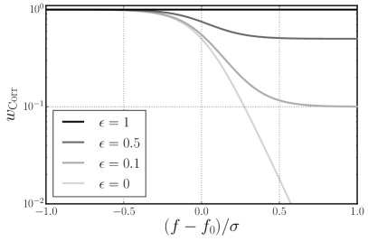
Figure 3: We illustrate the behavior of the function $w_{\rm corr}(f)$ in Eq. (9), which modifies the amplitude of the waveform with respect the one of a BNS and BBH. The central frequency $f_{0}$ determines the frequency at which the amplitude is tapered; the width $\sigma$ determines the range of frequencies over which the tapering takes place; the parameter $\epsilon$ keeps the post-merger signal at a suppressed level, if it is nonzero.

We then apply a correction to the amplitude that describes the tidal disruption effects discussed in the previous section. More precisely, we relate the amplitude of SEOBNR_NSBH, $A(f)$, to the amplitude of SEOBNR_BNS with no tapering or tidal amplitude corrections applied, $A_{\rm NRT-notaper}(f)$, via

$$A(f)=w_{\rm corr}(f)A_{\rm NRT-notaper}(f),$$ (9)

where the correction function $w_{\rm corr}$ is given by

$$w_{\rm corr}(f)=w^{-}(f;f_{0},\sigma)+\epsilon w^{+}(f;f_{0},\sigma),$$ (10)

and $w^{\pm}(f;f_{0},\sigma)$ are the hyperbolic-tangent window functions

$$w^{\pm}(f;f_{0},\sigma)=\frac{1}{2}\left[1\pm\tanh\left(\frac{4(f-f_{0})}{\sigma}\right)\right].$$ (11)

We illustrate the behavior of $w_{\rm corr}$ in Fig. 3. When $\epsilon=0$, $w_{\rm corr}(f)$ cuts off the amplitude before the end expected for a BBH system with the same masses and spins of the NSBH, and therefore describes tidal disruption. When $\epsilon>0$, the final part of the inspiral and the post-merger signal are still present, but are suppressed relative to the BBH case. The parameters $f_{0},\sigma,\epsilon$, which determine the precise nature of these corrections, are determined by comparing with NR simulations.

Following Ref. Pannarale et al. (2015b), we classify the waveforms into four cases: non-disruptive, disruptive, mildly disruptive without torus remnant, and mildly disruptive with torus remnant, depending on the intrinsic parameters of the system. To determine the three parameters {$f_{0},\sigma_{0},\epsilon$} in Eq. (9), we adapt the amplitude model of Ref. Pannarale et al. (2015b), which was developed for a different BBH baseline, to the SEOBNR_BBH model. We then calibrate the parameters of this model, using the method described in Sec. II.4.

Non-disruptive mergers: $f_{\rm RD}<f_{\rm tide},M_{\rm b,torus}=0$. When the tidal frequency is larger than the ringdown frequency of the final BH, the NS reaches the ISCO before crossing $r_{\rm tide}$. In this case the NS remains intact as it plunges, but with a slightly suppressed amplitude of the ringdown. The waveform is very similar to a BBH. To describe this, we use $f_{0}=f_{\rm ND},\sigma_{0}=\sigma_{\rm ND},\epsilon=\epsilon_{\rm ND}$, where ND stands for non-disruptive, and

$$w_{\rm ND}(f)=w^{-}(f;f_{\rm ND},\sigma_{\rm ND})+\epsilon_{\rm ND}w^{+}(f;f_{\rm ND},\sigma_{\rm ND}).$$ (12)

The explicit expressions relating $f_{\rm ND},\sigma_{\rm ND}$, and $\epsilon_{\rm ND}$ to the intrinsic parameters of the binary are given in Appendix A.

Disruptive mergers: $f_{\rm RD}>f_{\rm tide},M_{\rm b,torus}>0$. In this case, tidal disruption occurs and a remnant torus of matter forms. For such systems, the typical merger and ringdown stages present for BBHs are exponentially suppressed. To model this case, we set $\epsilon=0$, so that the waveform decays above a frequency $f_{\rm D}$ with width $\sigma_{\rm D}$. This leads to the expression

$$w_{\rm D}(f)=w^{-}(f;f_{\rm D},\sigma_{\rm D}).$$ (13)

The precise definition is given in Appendix A.

Mildly disruptive mergers with no torus remnant: $f_{\rm RD}>f_{\rm tide},M_{\rm b,torus}=0$. In this case, the NS undergoes mass shedding, but no torus forms around the remnant BH. We combine the information from the non-disruptive and disruptive cases to determine the cutoff frequency and the width of the tapering. We set $f_{0}=(1-Q^{-1})f_{\rm ND}+Q^{-1}f_{\rm tide},\sigma_{0}=(\sigma_{\rm D}+\sigma_{\rm ND})/2,\epsilon=0$.

Mildly disruptive mergers with torus remnant: $f_{\rm RD}<f_{\rm tide},M_{\rm b,torus}>0$. In this scenario the tidal frequency is above the ringdown frequency, but there is a remnant disk of matter around the BH. As discussed, for example, in Ref. Shibata and Taniguchi (2011), this scenario occurs at large BH spins, and represents the case in which the NS is disrupted before crossing the ISCO, but the size of the tidally disrupted material in the vicinity of the BH is smaller than the BH surface area. Thus, in this case, although a remnant disk eventually forms, the matter does not distribute uniformly around the BH quickly enough to cancel coherently or suppress the BH oscillations. As a consequence, the ending part of the NSBH waveform contains a ringdown signal. In this case, we again combine information from Cases 1 and 2, and fix $f_{0}=f_{\rm D},\sigma_{0}=\sigma_{\rm ND},\epsilon=\epsilon_{\rm ND}$.

In Fig. 2, we show the regions of these different parameter spaces, along with relevant NR simulations from the SACRA and SpEC codes.

II.4 Fitting procedure

The amplitude correction described in the previous section has 20 free parameters, which we denote with the vector $\vec{\lambda}$. The definition of these parameters is given in Appendix A. We fix the coefficients in $\vec{\lambda}$ by requiring that the SEOBNR_NSBH waveforms agree, as much as possible, with the SpEC and SACRA waveforms described in Sec. II.2.

Simulation	$f_{\rm low}$ [Hz]	SEOBNR_NSBH	PhenomNSBH
SXS:BHNS:0001	169	$7.5\times 10^{-3}$	$8.8\times 10^{-3}$
SXS:BHNS:0002	315	$6.0\times 10^{-3}$	$4.5\times 10^{-3}$
SXS:BHNS:0003	407	$5.5\times 10^{-3}$	$5.2\times 10^{-3}$
SXS:BHNS:0004	447	$7.8\times 10^{-3}$	$1.9\times 10^{-2}$
SXS:BHNS:0006	314	$5.6\times 10^{-3}$	$5.3\times 10^{-3}$
M12-7-S8-LS220	351	$6.9\times 10^{-3}$	$7.8\times 10^{-3}$
M12-7-S9-LS220	343	$1.1\times 10^{-2}$	$7.4\times 10^{-3}$
M12-10-S8-LS220	279	$8.4\times 10^{-3}$	$2.0\times 10^{-2}$
M12-10-S9-LS220	271	$1.1\times 10^{-2}$	$2.7\times 10^{-2}$
M14-7-S7-LS220	431	$1.6\times 10^{-2}$	$9.3\times 10^{-3}$
M14-7-S8-LS220	397	$1.1\times 10^{-2}$	$2.0\times 10^{-2}$
M14-7-S9-LS220	426	$1.7\times 10^{-2}$	$1.4\times 10^{-2}$
M14-10-S8-LS220	286	$1.1\times 10^{-2}$	$4.6\times 10^{-2}$
M14-10-S9-LS220	297	$1.1\times 10^{-2}$	$4.3\times 10^{-2}$
SXS:BHNS:0005	448	$7.4\times 10^{-2}$	$8.0\times 10^{-2}$
SXS:BHNS:0007	315	$7.3\times 10^{-3}$	$1.1\times 10^{-2}$
Q3S9	300	$8.2\times 10^{-3}$	$4.9\times 10^{-3}$
Q4S9	238	$1.0\times 10^{-2}$	$6.5\times 10^{-3}$

Table 3: We list the unfaithfulness between different waveform models and SXS NSBH simulations. To compute the unfaithulness we use the Advanced LIGO design sensitivity PSD. In the left columns we show the unfaithfulness between SEOBNR_NSBH and PhenomNSBH, and the NR simulations. We compute the mismatch integral starting at the lower frequency $f_{\rm low}$ listed; this corresponds to a time late enough in the waveform that effects of junk radiation and eccentricity are negligible. The simulations below the horizontal line indicate simulations with nonzero $\chi_{\rm NS}$. These simulations were not included in the calibration and are used for validation.

	Window		${\rm SEOBNR\_NSBH}$-Hybrid		PhenomNSBH-Hybrid
Simulation	$t_{\rm min}$ [s]	$t_{\rm max}$ [s]	SEOBNR_NSBH	PhenomNSBH	SEOBNR_NSBH	PhenomNSBH
SXS:BHNS:0001	0.01	0.025	$1.2\times 10^{-3}$	$1.2\times 10^{-2}$	$2.4\times 10^{-3}$	$1.3\times 10^{-2}$
SXS:BHNS:0002	0.01	0.025	$7.4\times 10^{-4}$	$1.3\times 10^{-4}$	$1.3\times 10^{-3}$	$1.4\times 10^{-4}$
SXS:BHNS:0003	0.005	0.018	$2.1\times 10^{-4}$	$1.6\times 10^{-4}$	$2.7\times 10^{-3}$	$1.3\times 10^{-3}$
SXS:BHNS:0004	0.008	0.02	$1.6\times 10^{-4}$	$5.7\times 10^{-4}$	$9.1\times 10^{-4}$	$2.7\times 10^{-4}$
SXS:BHNS:0006	0.01	0.025	$1.8\times 10^{-3}$	$1.9\times 10^{-3}$	$4.6\times 10^{-3}$	$3.9\times 10^{-4}$
M12-7-S8-LS220	0.008	0.026	$2.0\times 10^{-3}$	$1.8\times 10^{-2}$	$1.8\times 10^{-2}$	$4.2\times 10^{-3}$
M12-7-S9-LS220	0.01	0.03	$1.4\times 10^{-3}$	$5.0\times 10^{-3}$	$1.8\times 10^{-2}$	$3.2\times 10^{-3}$
M12-10-S8-LS220	0.01	0.04	$7.1\times 10^{-3}$	$1.9\times 10^{-2}$	$6.2\times 10^{-2}$	$1.4\times 10^{-2}$
M12-10-S9-LS220	0.01	0.04	$1.1\times 10^{-2}$	$2.9\times 10^{-2}$	$7.2\times 10^{-2}$	$2.5\times 10^{-2}$
M14-7-S7-LS220	0.0075	0.02	$9.1\times 10^{-4}$	$5.3\times 10^{-3}$	$5.5\times 10^{-3}$	$2.9\times 10^{-4}$
M14-7-S8-LS220	0.006	0.018	$3.7\times 10^{-4}$	$9.1\times 10^{-3}$	$2.6\times 10^{-3}$	$2.2\times 10^{-3}$
M14-7-S9-LS220	0.0075	0.02	$1.6\times 10^{-3}$	$3.7\times 10^{-3}$	$7.1\times 10^{-3}$	$3.3\times 10^{-4}$
M14-10-S8-LS220	0.005	0.03	$1.4\times 10^{-3}$	$2.4\times 10^{-2}$	$3.6\times 10^{-2}$	$4.3\times 10^{-3}$
M14-10-S9-LS220	0.007	0.03	$1.1\times 10^{-2}$	$6.5\times 10^{-2}$	$3.3\times 10^{-2}$	$4.3\times 10^{-3}$
SXS:BHNS:0005	0.005	0.015	$3.4\times 10^{-3}$	$4.0\times 10^{-2}$	$4.7\times 10^{-2}$	$3.6\times 10^{-3}$
SXS:BHNS:0007	0.005	0.055	$6.4\times 10^{-4}$	$1.9\times 10^{-2}$	$7.1\times 10^{-3}$	$1.2\times 10^{-3}$
Q3S9	0.01	0.025	$5.5\times 10^{-4}$	$1.2\times 10^{-2}$	$1.5\times 10^{-2}$	$3.3\times 10^{-4}$
Q4S9	0.01	0.025	$8.6\times 10^{-4}$	$2.4\times 10^{-3}$	$6.9\times 10^{-3}$	$2.4\times 10^{-3}$

Table 4: Unfaithfulness between the PhenomNSBH and SEOBNR_NSBH waveform models, and NR-hybrids constructed with these models. The details of the hybrid construction are given in the main text. We give here the initial $t_{\rm min}$ and final $t_{\rm max}$ times of the window used for hybridization in seconds, relative to the beginning of the NR data.

For a given NR waveform indexed by I, let us denote the Fourier-domain amplitude of the dominant mode by $A^{\rm NR}_{\rm I}(f;\vec{\theta})$. Given the intrinsic parameters of the binary, $\vec{\theta}$, and a set of fit parameters $\vec{\lambda}$, we compute the following quantity $\Delta_{\rm I}(\vec{\lambda})^{2}$,

$$\Delta_{\rm I}(\vec{\lambda})^{2}=\int_{f_{\rm min}}^{f_{\rm cut}}{\rm d}f\frac{\left[A(f;\vec{\theta},\vec{\lambda})-A_{\rm I}^{\rm NR}(f;\vec{\theta})\right]^{2}}{\sigma_{\rm I}(f)^{2}},$$ (14)

to estimate the difference between the frequency-domain amplitude of the model $A(f)$ and of the NR simulation $A_{\rm I}^{\rm NR}(f)$. We choose the lower bound of the integral $f_{\rm min}$ to be the frequency at which $A^{\rm NR}_{\rm I}(f)$ falls to 90% of its initial (lowest-frequency) value; this is a low enough frequency to ensure $w_{\rm corr}(f_{\rm min})\approx 1$ while avoiding possible contamination from eccentricity in the initial data. For the upper frequency, we take a definition inspired by the cutoff frequency given in Ref. Pannarale et al. (2015a). First, we define $f_{\rm max}$ to be the frequency at which $f^{2}A(f)$ takes its maximum value. Then we define $f_{\rm cut}$ to be the frequency (larger than $f_{\rm max}$) which satisfies

$$f_{\rm cut}A_{\rm I}^{\rm NR}(f_{\rm cut})=0.1f_{\rm max}A_{\rm I}^{\rm NR}(f_{\rm max}).$$ (15)

This frequency is larger than the ringdown frequency for non-disruptive mergers. For disruptive mergers, $f_{\rm cut}$ gives a characteristic frequency at which the frequency domain amplitude has been suppressed. For the error function in Eq. (14), we consider a constant relative error at each frequency given by $\sigma_{\rm I}(f)=k_{\rm I}A_{\rm I}(f)$. We use $k_{\rm I}=1$ for the SACRA waveforms, and $k_{\rm I}=0.1$ for the SpEC waveforms, to account for the difference in length and accuracy in the waveforms. We then compute a global error, for a given subset $\mathcal{S}$ of the NR waveforms, by summing $\Delta_{\rm I}^{2}$ over all NR waveforms in $\mathcal{S}$

$$\Delta^{2}(\vec{\lambda})=\sum_{\rm I\in\mathcal{S}}\Delta_{\rm I}^{2}(\vec{\lambda}).$$ (16)

We minimize $\Delta^{2}(\vec{\lambda})$ with respect to $\vec{\lambda}$ using the Nelder-Mead algorithm Nelder and Mead (1965). We first use the parameter values from Ref. Pannarale et al. (2015b) as an initial guess, and minimize the error over the parameters of the non-disruptive and disruptive window functions separately. We then use the results of this fit as an initial guess for a global fit, including all of the available waveforms in $\mathcal{S}$. The final results of this global fit are used to define the model, and the numerical values are given in Table 7 in Appendix A.

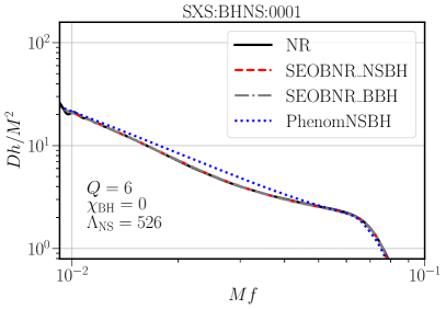
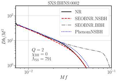
Figure 4: Frequency domain amplitude comparisons of SXS simulations, the NSBH waveform models SEOBNR_NSBH and PhenomNSBH, and the BBH model SEOBNR_BBH, that is used as a baseline for SEOBNR_NSBH. SEOBNR_NSBH is able to capture the effects of tidal disruption on the amplitude, while also reducing to BBH-like waveform for large mass ratios when tidal disruption does not occur.

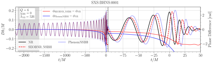
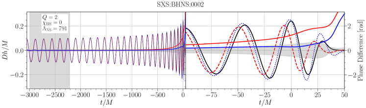
Figure 5: Time domain comparisons of 2 NR simulations in the time domain, along with SEOBNR_NSBH and PhenomNSBH. We show two of the publicly available SXS simulations with zero spin which were used for calibration of SEOBNR_NSBH: the non-disruptive merger SXS:BHNS:0001, with mass ratio 6, and the disruptive merger SXS:BHNS:0002 with mass ratio 2. Also plotted is the phase difference for both NSBH models against the relevant NR simulation. The gray band shows the region used to align the model waveforms and NR. We also show the NR phase error for SXS:BHNS:0002 as a horizontal gray band; for SXS:BHNS:0001, which is an older waveform, the NR error is not available. The NR waveform has been shifted in time so the peak amplitude occurs at $t=0$, and that the phase is zero there. We see that, for both waveform families, the agreement with NR is very good at the beginning of the NR waveform, but there is dephasing toward the end.

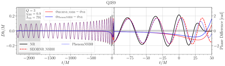
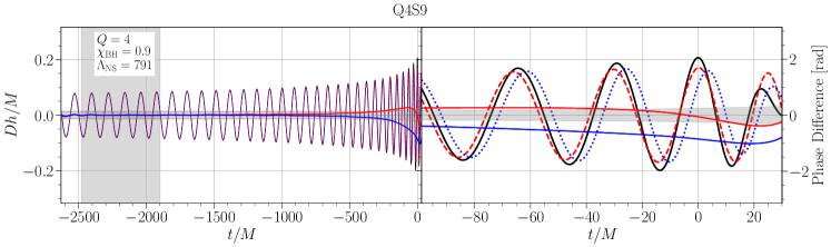
Figure 6: Time domain comparisons of highly accurate waveforms of disruptive mergers, as well as the models SEOBNR_NSBH and PhenomNSBH. We show Q3S9, with mass ratio 3, and Q4S9, with mass ratio 4. Both configurations have a dimensionless BH spin magnitude of 0.9. These waveforms were not used to calibrate SEOBNR_NSBH. We see excellent agreement across a large number of cycles. The time and phase of the NR waveform have been fixed as in Fig. 5.

We now turn to a quantitative assessment of the model’s performance by comparing against NR simulations. We additionally compare with the recently developed PhenomNSBH model of Ref. Thompson et al. (2020), in order to understand the performance of the two approximants relative to NR and to each other. To this end, we employ the faithfulness function given in Ref. Damour et al. (1998), which is commonly used in LIGO and Virgo data analysis to assess the agreement of two waveforms, e.g., the template $\tau$ and the signal $s$. Let us first introduce the inner product between two waveforms $a$ and $b$ Sathyaprakash and Dhurandhar (1991); Finn and Chernoff (1993)

$$\langle a|b\rangle\equiv 4{\rm Re}\int{\rm d}f\frac{a^{*}(f)\,b(f)}{S_{n}(f)},$$ (17)

where a star denotes the complex conjugate and $S_{n}(f)$ is the one-sided, power spectral density (PSD) of the detector noise. Here, we use the Advanced LIGO design sensitivity PSD as given in Ref. Barsotti et al. (2018). We compute the faithfulness $\mathcal{F}$ by maximizing the normalized inner product (or overlap) over the coalescence time $t_{c}$, the initial phase ${\phi_{0}}_{\tau}$ of the template $\tau$, and setting the phase of the signal ${\phi_{0}}_{s}$ to zero at merger, while fixing the same parameters $\vec{\theta}$ for the template and the signal, that is

$$\mathcal{F}\equiv{\rm max}_{t_{c},{\phi_{0}}_{\tau}}\left[\frac{\langle\tau|s\rangle}{\sqrt{\langle\tau|\tau\rangle\langle s|s\rangle}}\right]_{\left\{{\vec{\theta}}_{\tau}={\vec{\theta}}_{s},{\phi_{0}}_{s}=0\right\}}.$$ (18)

We find it convenient to discuss results also in terms of the unfaithfulness, that is $\bar{\mathcal{F}}=1-\mathcal{F}$. Henceforth, we consider the NR waveform as the signal, and the SEOBNR_NSBH or PhenomNSBH as the template. In Table 3 we list the unfaithfulness obtained against all the SXS NSBH waveforms at our disposal, for both SEOBNR_NSBH and PhenomNSBH. We also specify the lower frequency $f_{\rm low}$ used to compute the match. We see that both models have broadly similar performance.

Since the NR waveforms do not cover the entire bandwidth of the detector, we compute the faithfulness also between both NSBH waveform models, and NR hybrids. We construct hybrids with both SEOBNR_NSBH and PhenomNSBH, and compare both waveform models to the two hybrids. The four comparisons have two distinct purposes. First, the low frequency part of SEOBNR_NSBH and the SEOBNR_NSBH hybrid, and the PhenomNSBH and PhenomNSBH hybrid, are identical up to a shift in the time and phase of the waveform, so that the unfaithfulness of SEOBNR_NSBH with an SEOBNR_NSBH hybrid quantifies the error of the waveform model failing to capture the NR; the same is true of the unfaithfulness between PhenomNSBH and a PhenomNSBH hybrid. Second, comparing SEOBNR_NSBH with a PhenomNSBH hybrid, and vice versa, includes the error from the NR part of the waveform, and additionally the error of waveform modeling uncertainty. We show the results in Table 4. We note that the choice of hybrid affects the unfaithfulness: the unfaithfulness of SEOBNR_NSBH with PhenomNSBH hybrids tends to be larger than the unfaithfulness of PhenomNSBH with SEOBNR_NSBH hybrids.

To construct the hybrids, we follow the hybridization procedure given in Refs. Dietrich et al. (2019b, a). We first align the waveforms by adjusting the time and phase of SEOBNR_NSBH to maximize the overlap with the NR waveform, then we apply a Hann window to smoothly transition from the model to the NR waveform. We refer to the initial and final times of the alignment window as $t_{\rm min}$ and $t_{\rm max}$. These are chosen for each waveform to produce good agreement in the early part of the waveform. We provide the windows used in Table 4.

In Fig. 4, we compare the frequency-domain amplitude of the SEOBNR_NSBH model and PhenomNSBH against two publicly available non-spinning SXS waveforms which were used to calibrate SEOBNR_NSBH. For context, we additionally show the BBH baseline model, SEOBNR_BBH. For SXS:BHNS:0001, which is a non-disruptive merger, the amplitudes of the NR data, SEOBNR_BBH, SEOBNR_NSBH, and PhenomNSBH, agree well. For the disruptive merger SXS:BHNS:0002, SEOBNR_NSBH and PhenomNSBH capture the tapering of the amplitude due to tidal disruption. In Fig. 5, we compare SEOBNR_NSBH and PhenomNSBH to the same two NR simulations in the time domain. We include the NR error for those waveforms for which it is available, estimated using the methods described in Refs. Foucart et al. (2019a); Boyle et al. (2019). In Fig 6, we compare SEOBNR_NSBH and PhenomNSBH to the accurate spinning simulations simulations Q3S9 and Q4S9, which we use for validation. We align the waveforms using the same procedure to construct the hybrids. We perform these comparisons using the $N=3$ extrapolation order.

II.5 Regime of validity

Parameter	Calibration range	Suggested range of validity
$Q$	[1,6]	[1,100]
$M_{\rm NS}$	[1.2,1.4] $M_{\odot}$	[1,3] $M_{\odot}$
$\Lambda_{\rm NS}$	[130,4200]	[0,5000]
$\chi_{\rm BH}$	[-0.5,0.9]	[-0.9,0.9]

Table 5: Range of intrinsic parameters for which the SEOBNR_NSBH waveform model was calibrated, and in which we suggest the model can be used. The calibration range gives the region of parameter space for which there are NR simulations. The suggested range of validity is the range we suggest for using the waveform, as explained in the main text. We note that a real EOS relates $\Lambda_{\rm NS}$ and $M_{\rm NS}$, and $\Lambda_{\rm NS}$ is a rapidly decreasing function of $M_{\rm NS}$. The largest value of $\Lambda_{\rm NS}$ for a 1.4 $M_{\odot}$ NS among the simulations we use is 791. See the main text for more detailed discussion.

In Table 5, we provide the parameter space region of the simulations used for calibration. We also give a suggested regime of validity for use of our SEOBNR_NSBH  waveform model, which we justify as follows.

• Mass ratio $Q$. We take the lower limit for the mass ratio to be 1, given that in our fit we include NR simulations with these mass ratios. For large enough mass ratios, for any spin and $\Lambda_{\rm NS}$, the merger becomes non-disruptive and the model reduces to the SEOBNR_BBH waveform model. We have checked that there is always a range of parameter space at large mass ratios where this transition occurs, within the regime of validity of the model. Therefore we inherit the upper limit on $Q$ coming from SEOBNR_BBH, which is of 100.

• NS mass $M_{\rm NS}$. Based on expectations of the maximum NS mass from the nuclear EOS, we restrict the NS mass to be less than $3M_{\odot}$. We also suggest restricting the NS mass to be larger than $1M_{\odot}$, which is consistent with the range that we choose for the tidal parameter $\Lambda_{\rm NS}$.

• NS tidal-deformability $\Lambda_{\rm NS}$. We have verified that sensible waveforms are generated with $\Lambda_{\rm NS}$ varying from 0 up to 5000, and on this basis suggest the waveform model can be used in this range. We have also performed a calibration and comparison against available NR simulations to verify the model accurately describes simulations with tidal disruption, as we have described. However the available NR simulations have a more limited range of $\Lambda_{\rm NS}$, depending on the NS mass and equation of state, as seen in Fig. 2. Thus we caution that tidal disruption effects are uncertain for large $\Lambda_{\rm NS}$, in particular $\Lambda_{\rm NS}\gtrsim 1000$ for $1.4M_{\odot}$ NSs. Even this restricted range includes the bound $\Lambda_{\rm NS}<800$ for a $1.4M_{\odot}$ NS, obtained from measurements of GW170817 in Ref. Abbott et al. (2018b).

• BH spin $\chi_{\rm BH}$. In the fit we include simulations with positive spins as large as $0.9$, and negative spins as low as -0.5. Since negative spins tend to make the merger less disruptive (i.e., more BBH-like), in order to obtain a symmetric range we suggest $[-0.9,0.9]$ as a range for the spin.

• NS spin $\chi_{\rm NS}$. While we do not include simulations with NS spin in the fit, from PN theory we expect that the main effect of the spin enters via the beta parameter derived in Ref. Arun et al. (2009); here we use the formulation given in Eq A6 of Ref. Ng et al. (2018)

  $$\beta=\frac{113-76\eta}{12}\chi_{\rm eff}+\frac{76\delta}{12}\chi_{a}$$ (19)

  where $\eta=Q/(Q+1)^{2}$ is the symmetric mass ratio, $\chi_{a}=(\chi_{\rm BH}-\chi_{\rm NS})/2$ is the antisymmetric combination of aligned spins, $\delta=(Q-1)/(Q+1)$ is an antisymmetric combination of the masses, and the effective aligned spin parameter $\chi_{\rm eff}$ is given by

  $$\chi_{\rm eff}=\frac{M_{\rm BH}\chi_{\rm BH}+M_{\rm NS}\chi_{\rm NS}}{M_{\rm BH}+M_{\rm NS}}.$$ (20)

  Except for mass ratios close to 1 and small spins, $\beta$ is dominated by the BH spin. We also see reasonable agreement with simulations when the NS spin is nonzero, as shown in Table 3. We therefore recommend that the NS spin is bounded by the low-spin prior that has been used in the literature, e.g. Refs. Abbott et al. (2019a); Abbott et al. (2020a), $|\chi_{\rm NS}|<0.05$.

Through a thorough study, we have verified that the SEOBNR_NSBH waveforms look sensible in the region in which we suggest to use this model.

III Applications

Having constructed the SEOBNR_NSBH waveform model and checked that it agrees well with existing NR waveforms, we now apply the model to three data-analysis problems. In particular, in Sec. III.1, we compute the unfaithfulness of the SEOBNR_NSBH model against SEOBNR_BBH and SEOBNR_BNS models in order to obtain an estimate of the regions of parameter space where the advanced-detector network may be able to distinguish different source classes. In Sec. III.2, we perform a Bayesian parameter-estimation analysis in which we inject a synthetic NSBH signal (notably a disruptive NSBH merger) and infer the source’s properties and parameter’s biases when recovering it with the SEOBNR_NSBH model and the SEOBNR_BBH model. Finally, in Sec. III.3, we reanalyze the LIGO/Virgo event GW170817 under the hypothesis that it is a NSBH binary, instead of a BNS.

III.1 Distinguishing different source classes

When is it possible to determine whether a given binary system is a BBH, BNS, or NSBH based on tidal effects in the gravitational waveform? We can address this question with our waveform model by considering how similar a SEOBNR_NSBH waveform is to a waveform from another source class. In this section we do not use an astrophysical prior on the masses of the objects to distinguish the source classes. Reference Hannam et al. (2013) considered the issue of distinguishing source classes, using measurements on the masses of the component objects, and an astrophyiscal prior on the masses of NSs and BHs, rather than measurements of the tidal parameter which we consider here. The conclusion of that work is that it will be difficult to distinguish different source classes with Advanced LIGO, with signals with SNRs in the range 10-20.

First, we consider the case of distinguishing the hypotheses that a given signal is a BBH or a NSBH. Suppose the signal is a NSBH with a given set of parameters, $\vec{\theta}_{\rm NSBH}$. We compute the unfaithfulness between the SEOBNR_NSBH and SEOBNR_BBH models, with the same masses and spins. In the left panel of Fig., 7, we show contours of the unfaithfulness in the $Q\mbox{--}\Lambda_{\rm NS}$ plane, for a $1.4M_{\odot}$ NS and $\chi_{\rm NS}=0$, while varying $\chi_{\rm BH}$ over the range $\{0,0.5,0.9\}$. To put the results in context, following Refs. Lindblom et al. (2008), we estimate that two waveforms are distinguishable at the $1\mbox{--}\sigma$ level when the signal-to-noise ratio (SNR) $\rho$ satisfies $\bar{\mathcal{F}}=K/2\rho^{2}$, where $K$ depends on the number of intrinsic parameters, $D$. Reference Chatziioannou et al. (2017) provides an estimate of $K=D-1$, at which the $D$-dimensional posteriors do not overlap at the 1-$\sigma$ level. Then, an unfaithfulness of $\bar{\mathcal{F}}=10^{-3}$, corresponds to an SNR of $\rho\approx 45$. However, this criterion does not apply directly to marginalized posteriors. A more detailed discussion of the use of this criterion can be found in Ref. Pürrer and Haster (2019). In particular, the value of $K$ at which systematic errors become comparable to statistical ones, depend on what parameter is being considered, as well as extrinsic parameters such as the inclination. They find that, when applying the criterion to marginalized posteriors, the estimate $K=D-1$ is conservative. Therefore, we emphasize that this criterion is sufficient, but it is not necessary, and also it does not say which parameters are biased and by how much.

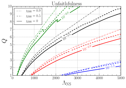
Figure 7: Contours with constant unfaithfulness in the $Q-\Lambda_{\rm NS}$ plane for varying BH spin $\chi_{\rm BH}$, when comparing SEOBNR_BBH and SEOBNR_NSBH assuming the Advanced LIGO design sensitivity PSD. As discussed in the main text, the unfaithfulness can be used to provide an estimate of the SNR at which data can be used to distinguish between two waveforms. Note that it is easier to distinguish BBH and NSBH systems for smaller $Q$ and larger $\chi_{\rm BH}$.

We also compute the unfaithfulness between the SEOBNR_NSBH and SEOBNR_BNS models, with the same masses, spins, and tidal parameters. We find that, for zero spin, the unfaithfulness between NSBH and BNS are always less than $10^{-3}$ when the NS mass is less than $3M_{\odot}$. This suggests it will be very difficult to distinguish NSBH and BNS systems on the basis of tidal effects on the waveform alone. However, inference on the component masses provides additional useful information that can help distinguish different source classes.

As said above, computing the unfaithfulness does not allow us to quantify its impact on the inference of the parameters of the binary, and quantify possible biases. Therefore, in the next section, at least for one particular case, we perform a Bayesian parameter-estimation study and extract those biases, and compare with the distinguishability criterion of Refs. Lindblom et al. (2008); Chatziioannou et al. (2017).

III.2 Parameter-estimation case study

In this section, because of computational costs, we perform a Bayesian parameter-estimation analysis for one specific NSBH system, and postpone to the future a more comprehensive analysis.

We first create a synthetic NSBH signal consisting of an NR hybrid built by stitching together the SEOBNR_NSBH  waveform to the SXS:BHNS:0006 waveform, with masses $M_{\rm BH}=2.1M_{\odot}$, $M_{\rm NS}=1.4M_{\odot}$, mass ratio $Q=1.5$, and both spins equal to zero. We do not add a noise realization (i.e., we work in zero noise) which is equivalent to averaging over different noise realizations, as shown in Ref. Nissanke et al. (2010). We perform four injections, with SNRs of 25, 50, 75, and 100 in the advanced LIGO-Virgo network. While the masses are not astrophysically motivated, this system is interesting to study because it is disruptive, and due to the mass ratio the tidal dephasing is enhanced. Further, SXS:BHNS:0006 is the simulation with the largest number of cycles of the publicly available SXS waveforms.

We apply the Markov Chain Monte Carlo (MCMC) sampling algorithm implemented in LALInference Veitch et al. (2015) to these four signals, and recover the signal with both the SEOBNR_BBH and SEOBNR_NSBH waveform models. Due to limited computational resources, we run the parameter estimation with a lower cutoff frequency of 30 Hz. We take the higher cutoff frequency to be 2048 Hz. We use a uniform prior on the detector frame component masses. For SEOBNR_NSBH, we impose a constraint that $M_{\rm NS}<3M_{\odot}$, $|\chi_{\rm NS}|<0.05$, and $|\chi_{\rm BH}|<0.9$ consistent with the range of validity of the model. We take a prior on $\Lambda_{\rm NS}$ that is uniform between 0 and 5000. For SEOBNR_BBH, we do not impose a constraint on the maximum mass but do require that the spins of both objects were less than 0.9. Since the two approximants make different assumptions about the nature of the component objects, in describing the results of the Bayesian analysis, we refer to the masses as $m_{1}$ and $m_{2}$ rather than $M_{\rm BH}$ and $M_{\rm NS}$.

In Fig. 8, we show posteriors in the $m_{1}-m_{2}$ plane, as well as the $q-\chi_{\rm eff}$ plane, for the SNR=25 and SNR=75 injections. For ease of comparison with other PE results by LIGO-Virgo analyses, we show the posterior in terms of the mass ratio $q\equiv Q^{-1}=m_{2}/m_{1}$. For the SNR=25 injection, we see the posteriors from the two waveforms agree very well and are consistent with the injected value within the 90% credible interval. For larger SNRs, posteriors derived using the two waveforms are in tension, and at large enough SNR, the injected value lies outside of the 90% credible interval of the posterior for each model. For the SNR=50 injection, and for larger SNRs, there is a bias in the masses and $\chi_{\rm eff}$ recovered using SEOBNR_BBH. In particular, SEOBNR_BBH recovers a larger total mass. The biases in the mass are due to the lack of tidal effects in SEOBNR_BBH. To quantify this, we have performed a run with two modified versions of SEOBNR_NSBH. The first modified model has a tidal phase correction but the same amplitude as SEOBNR_BBH. The second one has the tidal disruption correction to the amplitude but no tidal phase is applied. At SNR=25, both models recover the injected mass ratio inside of the 90% credible interval. At SNR=75, we find that the first modified model, like SEOBNR_NSBH, obtains the correct value within the 90% interval. On the other hand, the second model, with only the amplitude correction, does not. This is consistent with the fact that the tidal phase accumulates over many cycles, while the merger frequency is at relatively high frequencies outside of the most sensitive band of the detector. The masses and spins recovered by SEOBNR_NSBH are consistent at the 90% level with the injected values for the SNR=50 case, but are only marginally consistent for the SNR=75 injection, and for SNR=100, the injected values of the masses and $\chi_{\rm eff}$ lie outside 90% credible interval. This bias is due to differences with the NR-hybrid waveform. We show the recovery of the SNR=75 injection, for which the SEOBNR_NSBH recovery is marginally consistent with the true parameters, in the right two panels of Fig. 8.

In Fig. 9, we show recovery of the tidal parameter $\Lambda_{\rm NS}$ obtained using SEOBNR_NSBH for the 4 different cases. In all four scenarios, the injected tidal parameter is consistent with the 90% credible interval of the $\Lambda_{\rm NS}$ posterior, although this is only marginally true for the SNR=100 injection. It is interesting to compare the difference between the recovered and injected values, with what is expected from the indistinguishability criterion discussed in the previous section. The unfaithfulness from 30 Hz between the NR hybrid used and SEOBNR_NSBH is $2\times 10^{-3}$, using the advanced LIGO design sensitivity PSD. From the indistinguishability criterion of Ref. Chatziioannou et al. (2017) discussed in the previous section, we would expect to see deviations at the $1-\sigma$ level between the posterior recovered with SEOBNR_NSBH and the injected value an SNR of 32. A full Bayesian analysis reveals that this level of bias for the recovery of $\tilde{\Lambda}$ only arises at a larger value of the SNR. However as we have emphasized, the criterion strictly applies only to the full $D$ dimensional posterior, and not the marginalized posteriors we consider in this section. Additionally, the criterion is only sufficient, it does not specify which parameters are biased, depends on extrinsic parameters such as the inclination, and it has been shown to be quite conservative when applied to the marginalized posteriors Pürrer and Haster (2019).

This case study illustrates the importance of having accurate NSBH models that can account for tidal disruption in order to derive correct conclusions about astrophysical parameters. However, we emphasize that these injections are only meant as an example. Larger mass ratios may be less tidally disruptive and have tidal effects on the phase suppressed. Conversely, systems with large BH spin will tend to be more disruptive, which will enhance the differences between the BBH and NSBH waveforms.

After this manuscipt was submitted, Ref. Huang et al. (2020) appeared as a preprint. This work provides a detailed parameter estimation study, recovering many different NSBH injections using SEOBNR_NSBH, PhenomNSBH, SEOBNR_BBH, SEOBNR_BNS, and other waveform models. The injected waveforms are hybrids of SXS:BHNS:0001, SXS:BHNS:0003, and SXS:BHNS:0004, with the NR surrogate model NRHybSur3dq8Tidal, developed in Ref. Barkett et al. (2019), at SNR=30 and SNR=70. Of the cases they study, SXS:BHNS:0004, with $M_{\rm NS}=M_{\rm BH}=1.4M_{\odot}$, has the most similar parameters to the signal we consider in this work. The results that Ref. Huang et al. (2020) obtains for SXS:BHNS:0004 are broadly similar to the results we present here. When SNR=30, the injected masses are recovered within the 90% credible intervals when recovering with SEOBNR_BBH, SEOBNR_BNS, SEOBNR_NSBH, and PhenomNSBH. When SNR=70, the component masses recovered using SEOBNR_BBH are biased towards larger values. On the other hand, the posteriors obtained with SEOBNR_BNS, SEOBNR_NSBH  and PhenomNSBH recover the component masses within the 90% credible interval. The fact that SEOBNR_BNS and SEOBNR_NSBH both recover the correct mass may indicate that the tidal phase is more important than the tidal disruption frequency for recovering the masses. For the tidal parameter, at SNR=70, the authors find that the recovery of SEOBNR_NSBH  as well as SEOBNR_BNS, is in tension at the 90% level. Interestingly, PhenomNSBH recovers the correct tidal parameter when SNR=70. This paper, like the current work, illustrates the need for accurate NSBH models as the detector network sensitivity improves.

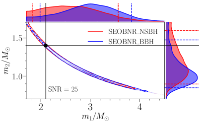
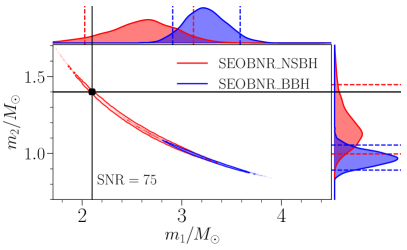
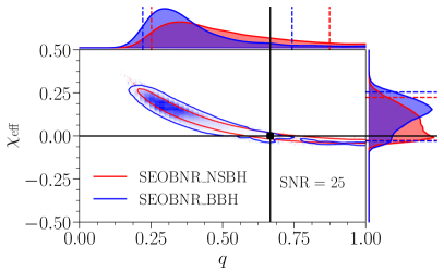
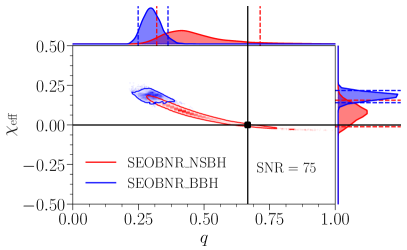
Figure 8: Illustrative parameter-estimation results for the SXS:BHNS:0006 hybrid injections described in the main text. In the top two panels, we show posterior distributions and 90% credible intervals for the component masses, with the posteriors derived using the SEOBNR_NSBH (SEOBNR_BBH) approximant in red (blue). In the bottom panels, we show the $q-\chi_{\rm eff}$ plane. We show the injected value as a black dot. For SNR=25, both SEOBNR_NSBH and SEOBNR_BBH recover the injected value within the 90% credible interval. For larger SNRs, the recovery with SEOBNR_BBH is biased. The posterior with the BBH waveform is peaked around a larger total mass, than the injected one. We show this explicitly for SNR=75. Additionally, we use this software injection test to explore how the difference between SEOBNR_NSBH and the NR hybrid affects parameter estimation. We see that, at SNR=75, the injected values of the masses and $\chi_{\rm eff}$ are marginally consistent with the SEOBNR_NSBH posterior at the 90% level; at larger SNRs we find the 90% credible interval does not include the true value.

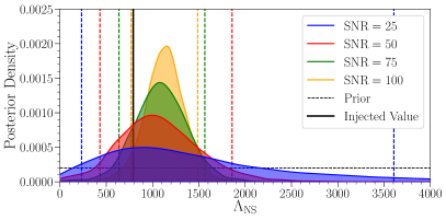
Figure 9: Posteriors for the NS tidal deformability $\Lambda_{\rm NS}$ for the NSBH hybrid injections described in the main text, recovered with SEOBNR_NSBH, for different SNRs. The recovered values of $\Lambda_{\rm NS}$ are consistent with the true value from the hybrid at the 90% level, however this is only marginally true for SNR=100.

III.3 Inference of GW170817 as a NSBH

As a final application, we reanalyze GW170817 Abbott et al. (2017b) under the hypothesis that it is a NSBH (see also Ref. Hinderer et al. (2019); Coughlin and Dietrich (2019) for related studies). Indeed, it is interesting to ask whether GW data alone can be used to distinguish the hypotheses that this event is a BNS or a NSBH.

We run the Bayesian inference study with the MCMC code implemented in LALInference, using publicly available data of GW170817 from the GW open science center (GWOSC) Vallisneri et al. (2015) (discussion of these data for O1 and O2 are contained in Ref. Abbott et al. (2019b)). We run with both the SEOBNR_NSBH model, as well as the SEOBNR_BNS model in order to be able to do a fair comparison. As far as we know, this is the first time that the new version of the SEOBNR_BNS model has been used to analyze GW170817. We compare our results to those from the runs obtained in the GWTC-1 catalog Abbott et al. (2019a), which used a former version of the SEOBNR_BNS model. We use the same priors as the GWTC-1 analysis Abbott et al. (2019a), except where otherwise stated. For SEOBNR_BNS we assume a flat prior on $\Lambda_{1}$ and $\Lambda_{2}$, while for SEOBNR_NSBH we assume a flat prior on $\Lambda_{2}$ and fix $\Lambda_{1}$ to zero. The posteriors contain support only in the interior of the prior domain for both waveform models with these priors. The prior on the component mass ranges from $0.5-7.7M_{\odot}$, and therefore the prior does not require that both objects have masses below the maximum mass of a NS.

First, we obtain that the median-recovered matched-filter SNR for each waveform model is $32.7$. Since the SEOBNR_NSBH and SEOBNR_BNS models recover the signal with a similar SNR, we do not find a clear preference either for a NSBH or BNS signal, when we only consider the GW data. Moreover, in Fig. 10, we show the recovery of the mass ratio and tidal deformability $\tilde{\Lambda}$ which is given by

$$\tilde{\Lambda}=\frac{16}{13}\frac{(m_{1}+12m_{2})m_{1}^{4}\Lambda_{1}+(m_{2}+12m_{1})m_{2}^{4}\Lambda_{2}}{(m_{1}+m_{2})^{5}}.$$ (21)

In order to more easily compare with results in Ref. Abbott et al. (2019a), we show the mass ratio $q\equiv Q^{-1}=M_{\rm NS}/M_{\rm BH}$. There is a preference for unequal mass ratios in the SEOBNR_NSBH  case, due to tidal disruption that occurs for higher mass ratios. Since $\tilde{\Lambda}$ depends non-trivially on the mass ratio and individual tidal parameters, and since $\Lambda_{1}$ is fixed to zero in the prior for SEOBNR_NSBH but not for the BNS models, the priors on $\tilde{\Lambda}$ for the BNS and NSBH models are quite different. In order to make a fair comparison between the posteriors on $\tilde{\Lambda}$, we divide each posterior by the prior on $\tilde{\Lambda}$, effectively obtaining a flat prior on $\tilde{\Lambda}$, as was done in Ref. Abbott et al. (2019a). We give the median and 90% credible intervals for the masses, $\chi_{\rm eff}$, $\tilde{\Lambda}$, and matched filter network SNR, in Table 6.

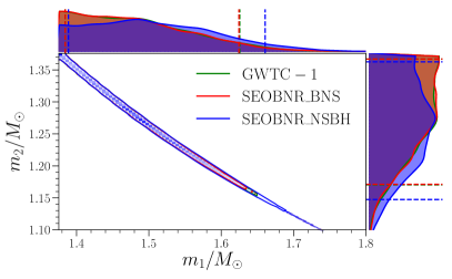
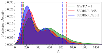
Figure 10: Reanalysis of GW170817. We show posteriors for the effective tidal deformability $\tilde{\Lambda}$ and the mass ratio $q\equiv m_{2}/m_{1}$, for three waveform models: in green we show the recovery with an older version of SEOBNR_BNS which performed in GWTC-1. In red we show a recovery with the current version of SEOBNR_BNS, which has been recalibrated in Ref. Dietrich et al. (2019a). The results are broadly consistent, though there are small differences consistent with changes to the waveform model. Finally, in blue we show the recovery with SEOBNR_NSBH. The NSBH model has a slight preference for less equal mass ratio. Note that we have reweighted the samples by dividing by the prior on $\tilde{\Lambda}$, as done in Ref. Abbott et al. (2019a).

Approximant	$m_{1}/M_{\odot}$	$m_{2}/M_{\odot}$	$\chi_{\rm eff}/10^{-3}$	$\tilde{\Lambda}$	Matched Filter SNR
SEOBNR_BNS (GWTC-1 version)	$1.47^{+0.15}_{-0.09}$	$1.28^{+0.08}_{-0.11}$	$3.4^{+14}_{-8}$	$456^{+565}_{-307}$	$32.7^{+0.1}_{-0.1}$
SEOBNR_BNS (current version)	$1.47^{+0.15}_{-0.09}$	$1.28^{+0.08}_{-0.11}$	$3.6^{+14}_{-8}$	$345^{+545}_{-217}$	$32.7^{+0.1}_{-0.1}$
SEOBNR_NSBH	$1.50^{+0.16}_{-0.11}$	$1.26^{+0.10}_{-0.11}$	$3.4^{+17}_{-9}$	$301^{+518}_{-189}$	$32.7^{+0.1}_{-0.1}$

Table 6: Median value and 90% credible region for parameters during a reanalysis of GW170817 with SEOBNR_NSBH and SEOBNR_BNS. The 3 PE runs give consistent results without a strong preference for BNS or NSBH based on GW data alone. The NSBH recovery appears to have a slight preference for unequal mass ratios and a smaller effective tidal deformability $\tilde{\Lambda}$ compared to the BNS recoveries.

IV Conclusion

In this work we have built an aligned-spin NSBH waveform model based on the EOB framework Buonanno and Damour (1999, 2000); Damour et al. (2000), the NRTidal approach Dietrich et al. (2017); Dietrich et al. (2019a) and NR simulations Foucart et al. (2013c); Foucart et al. (2019a, 2014); Kyutoku et al. (2010, 2011): SEOBNR_NSBH. In building the model, we have used final mass and spin fits from Ref. Zappa et al. (2019), the $\Lambda_{\rm NS}-C_{\rm NS}$ relations of Ref. Yagi and Yunes (2017), and fits for the disk mass from Ref. Foucart (2012). This model incorporates a suitable tapering of the frequency-domain waveform’s amplitude in regions where tidal disruption occurs building on the amplitude model of Ref. Pannarale et al. (2015b), as evinced from physical considerations of tidal effects as the NS plunges into the BH, and from NR simulations of those sources. Tidal corrections to the frequency-domain waveform’s phase have been computed using the NRTidal framework. We have shown that SEOBNR_NSBH gives good agreement with NR simulations by comparing the waveforms in the frequency domain (Fig. 4) and time domain (Fig. 5), as well as by computing the unfaithfulnesses shown in Tables 3 and  4. In Fig. 6, we compare the model with two new, highly accurate, simulations from the SXS Collaboration of disruptive NSBHs with highly spinning BHs, which we used for validation. We find very good agreement across a large number of cycles. We also performed the same comparisons with the recently published model PhenomNSBH, and find similar levels of agreement with NR. In Figs. 8 and 9, we have demonstrated that the model can be used to infer properties of NSBH systems using software injections, and that at large enough SNR assuming the wrong source class can lead to biased astrophysical inferences. Finally, we have reanalyzed GW170817 with the hypothesis that it is a NSBH instead of a BNS. In Table 6, we see the results are broadly consistent, although there seems to be a slight preference for smaller tidal deformability and unequal masses when recovering with SEOBNR_NSBH.

In the future, we plan to extend and improve the SEOBNR_NSBH waveform model in various ways. A relatively simple, but important extension is to incorporate information from modes beyond the quadrupolar one using SEOBNRv4HM Cotesta et al. (2018) as a baseline. This is particularly relevant, since the NS can be tidally disrupted also in cases in which the mass ratio is larger than one and the BH spin is large. Another crucial improvement is to extend the model to precessing NSBH binaries, since some astrophysical scenarios predict that the BH spin may be misaligned with respect to the orbital angular momentum. As more high quality NR simulations of NSBHs become available, it will also be possible to develop a more accurate model for the transition from disruptive to non-disruptive mergers. It will also be interesting to study the effect of using different tidal models in order to quantify uncertainty in the tidal part of the waveform. Finally, as we have mentioned, there is currently no model that smoothly covers the full range of source classes: BBH, NSBH, and BNS. Building a model which can capture all of relevant physics is an important future goal.

Appendix A Explicit form of amplitude correction

The amplitude corrections are parameterized based on the model presented in Ref. Pannarale et al. (2015b). We use the same parametric form for each component of the amplitude correction, and refit the coefficients. We have streamlined the notation.

A.1 Non-disruptive

The non-disruptive window function given in Eq. 12 contains the parameters $f_{\rm ND}$, $\sigma_{\rm ND}$, and $\epsilon_{\rm ND}$, which we compute as

$$f_{\rm ND} = f_{\rm RD},$$ (22a)

$$\sigma_{\rm ND} = \bar{\sigma}_{\rm ND}+2w^{-}(x;x_{0},\sigma_{x}),$$ (22b)

$$\epsilon_{\rm ND} = w^{+}(y;y_{0},\sigma_{y}),$$ (22c)

where $f_{\rm RD}$ is the ringdown frequency, which we estimate in terms of the final mass and spin using the fits from Ref. Berti et al. (2006). Following Refs. Pannarale et al. (2013); Pannarale et al. (2015b), we have introduced $x$ and $y$, which are a measure of how close the merger is to becoming disruptive. These quantities appear inside of window functions in order to ensure that the corrections to the ringdown are smoothly turned off ($\epsilon_{\rm ND}\rightarrow 0,\sigma_{\rm ND}\rightarrow\infty$) as the merger becomes less disruptive and therefore more like a BBH. For large $\sigma_{\rm ND}$ and $\epsilon_{\rm ND}$ on the intrinsic parameters of the binary. are determined by the tidal frequency, ringdown frequency, NS compactness, and BH spin via

$$x = \left(\frac{f_{\rm RD}-f_{\rm tide}}{f_{RD}}\right)^{2}+x_{C}C_{\rm NS}+x_{\chi}\chi_{\rm BH},$$ (23a)

$$y = \left(\frac{f_{\rm RD}-f_{\rm tide}}{f_{RD}}\right)^{2}+y_{C}C_{\rm NS}+y_{\chi}\chi_{\rm BH}.$$ (23b)

The nine coefficients $\{\bar{\sigma}_{\rm ND},x_{0},\sigma_{x},x_{C},x_{\chi},y_{0},\sigma_{y},y_{C},y_{\chi}\}$ were determined by a fitting procedure as described in Sec. II.4. Their values are given in Table 7.

A.2 Disruptive

The disruptive window correction in Eq. 13 is defined in terms of $f_{\rm D}$ and $\sigma_{\rm D}$, which we parameterize as

$$f_{\rm D} = \Big{(}a_{0}+a_{M}\frac{M_{\rm b,torus}}{M_{\rm b,NS}}+a_{C}C_{\rm NS}+a_{\nu}\sqrt{\nu}+a_{\chi}\chi\Big{)}f_{\rm tide}$$

$$\sigma_{\rm D} = b_{0}+b_{M}\frac{M_{\rm b,torus}}{M_{\rm b,NS}}+b_{C}C_{\rm NS}+b_{\nu}\sqrt{\nu}+\sum_{k=1}^{3}b^{(k)}_{\chi}\chi^{k}.$$

In this expression, there are twelve coefficients $\{a_{0},a_{M},a_{C},a_{\nu},a_{\chi},b_{0},b_{M},b_{C},b_{\nu},b_{\chi}^{(1)},b_{\chi}^{(2)},b_{\chi}^{(3)}\}$ which were determined by a fitting procedure as described in Sec. II.4. Their values are given in Table 7. As in the case of Ref. Pannarale et al. (2015b), we find that the parameters $b_{\chi}^{(1)},b_{\chi}^{(2)},b_{\chi}^{(3)}$ do not decrease monotonically.

Parameter	Value
$\bar{\sigma}_{\rm ND}$	0.0225006
$x_{0}$	-0.0923660
$\sigma_{x}$	0.0187155
$x_{C}$	-0.486533
$x_{\chi}$	-0.0314394
$y_{0}$	-0.177393
$\sigma_{y}$	0.771910
$y_{C}$	0.493376
$y_{\chi}$	0.0569155
$a_{0}$	1.27280
$a_{M}$	-1.68735
$a_{C}$	-1.43369
$a_{\nu}$	-0.510033
$a_{\chi}$	0.280002
$b_{0}$	0.185326
$b_{M}$	-0.253476
$b_{C}$	0.251061
$b_{\nu}$	-0.284595
$b_{\chi}^{(1)}$	-0.000757100
$b_{\chi}^{(2)}$	0.018089075
$b_{\chi}^{(3)}$	0.028545184

Table 7: Parameters for the amplitude correction $w_{\rm corr}(f)$. The parameters above the line appear in the correction for tidally disruptive mergers, the parameters below the line appear in the correction for disruptive mergers.

References

- Aasi et al. (2015) J. Aasi et al. (LIGO Scientific), Class. Quant. Grav. 32, 074001 (2015).
- Acernese et al. (2015) F. Acernese et al. (Virgo), Class. Quant. Grav. 32, 024001 (2015).
- Abbott et al. (2019a) B. P. Abbott et al. (LIGO Scientific, Virgo), Phys. Rev. X9, 031040 (2019a).
- Abbott et al. (2020a) B. Abbott et al. (LIGO Scientific, Virgo) (2020a), eprint 2001.01761.
- Venumadhav et al. (2019) T. Venumadhav, B. Zackay, J. Roulet, L. Dai, and M. Zaldarriaga (2019), eprint 1904.07214.
- Zackay et al. (2019a) B. Zackay, T. Venumadhav, L. Dai, J. Roulet, and M. Zaldarriaga, Phys. Rev. D 100, 023007 (2019a).
- Zackay et al. (2019b) B. Zackay, L. Dai, T. Venumadhav, J. Roulet, and M. Zaldarriaga (2019b), eprint 1910.09528.
- Abadie et al. (2010) J. Abadie et al. (LIGO Scientific, Virgo), Class. Quant. Grav. 27, 173001 (2010).
- Abbott et al. (2018a) B. P. Abbott et al. (KAGRA, LIGO Scientific, Virgo), Living Rev. Rel. 21, 3 (2018a), eprint 1304.0670v10.
- LIGO Scientific Collaboration, Virgo Collaboration (2019a) LIGO Scientific Collaboration, Virgo Collaboration, GCN 25324 (2019a), URL https://gcn.gsfc.nasa.gov/gcn3/25324.gcn3.
- LIGO Scientific Collaboration, Virgo Collaboration (2019b) LIGO Scientific Collaboration, Virgo Collaboration, GCN 25549. (2019b), URL https://gcn.gsfc.nasa.gov/gcn3/25549.gcn3.
- LIGO Scientific Collaboration, Virgo Collaboration (2019c) LIGO Scientific Collaboration, Virgo Collaboration, GCN 25695 (2019c), URL https://gcn.gsfc.nasa.gov/gcn3/25695.gcn3.
- LIGO Scientific Collaboration, Virgo Collaboration (2019d) LIGO Scientific Collaboration, Virgo Collaboration, GCN 25814 (2019d), URL https://gcn.gsfc.nasa.gov/gcn3/25814.gcn3.
- LIGO Scientific Collaboration, Virgo Collaboration (2019e) LIGO Scientific Collaboration, Virgo Collaboration, GCN 25876 (2019e), URL https://gcn.gsfc.nasa.gov/gcn3/25876.gcn3.
- LIGO Scientific Collaboration, Virgo Collaboration (2019f) LIGO Scientific Collaboration, Virgo Collaboration, GCN 26350 (2019f), URL https://gcn.gsfc.nasa.gov/gcn3/26350.gcn3.
- LIGO Scientific Collaboration, Virgo Collaboration (2020) LIGO Scientific Collaboration, Virgo Collaboration, GCN 26640 (2020), URL https://gcn.gsfc.nasa.gov/gcn3/26640.gcn3.
- Hinderer et al. (2019) T. Hinderer et al., Phys. Rev. D100, 06321 (2019).
- Coughlin and Dietrich (2019) M. W. Coughlin and T. Dietrich, Phys. Rev. D100, 043011 (2019).
- Abbott et al. (2020b) B. P. Abbott et al. (LIGO Scientific, Virgo), Class. Quant. Grav. 37, 045006 (2020b).
- Han et al. (2020) M.-Z. Han, S.-P. Tang, Y.-M. Hu, Y.-J. Li, J.-L. Jiang, Z.-P. Jin, Y.-Z. Fan, and D.-M. Wei, Astrophys. J. 891, L5 (2020).
- Kyutoku et al. (2020) K. Kyutoku, S. Fujibayashi, K. Hayashi, K. Kawaguchi, K. Kiuchi, M. Shibata, and M. Tanaka, Astrophys. J. 890, L4 (2020), eprint 2001.04474.
- Shibata and Taniguchi (2011) M. Shibata and K. Taniguchi, Living Rev. Rel. 14, 6 (2011).
- Flanagan (1998) É. É. Flanagan, Phys. Rev. D58, 124030 (1998).
- Flanagan and Hinderer (2008) É. É. Flanagan and T. Hinderer, Phys. Rev. D77, 021502 (2008).
- Vines and Flanagan (2013) J. E. Vines and É. É. Flanagan, Phys. Rev. D88, 024046 (2013).
- Pannarale et al. (2011a) F. Pannarale, L. Rezzolla, F. Ohme, and J. S. Read, Phys. Rev. D 84, 104017 (2011a), eprint 1103.3526.
- Kyutoku et al. (2010) K. Kyutoku, M. Shibata, and K. Taniguchi, Phys. Rev. D82, 044049 (2010), [Erratum: Phys. Rev.D84,049902(2011)].
- Foucart et al. (2013a) F. Foucart, L. Buchman, M. D. Duez, M. Grudich, L. E. Kidder, I. MacDonald, A. Mroue, H. P. Pfeiffer, M. A. Scheel, and B. Szilagyi, Phys. Rev. D88, 064017 (2013a).
- Foucart et al. (2011) F. Foucart, M. D. Duez, L. E. Kidder, and S. A. Teukolsky, Phys. Rev. D83, 024005 (2011).
- Kyutoku et al. (2011) K. Kyutoku, H. Okawa, M. Shibata, and K. Taniguchi, Phys. Rev. D84, 064018 (2011).
- Foucart et al. (2013b) F. Foucart, M. B. Deaton, M. D. Duez, L. E. Kidder, I. MacDonald, C. D. Ott, H. P. Pfeiffer, M. A. Scheel, B. Szilagyi, and S. A. Teukolsky, Phys. Rev. D87, 084006 (2013b).
- Kawaguchi et al. (2015) K. Kawaguchi, K. Kyutoku, H. Nakano, H. Okawa, M. Shibata, and K. Taniguchi, Phys. Rev. D 92, 024014 (2015), eprint 1506.05473.
- Pannarale et al. (2011b) F. Pannarale, A. Tonita, and L. Rezzolla, Astrophys. J. 727, 95 (2011b), eprint 1007.4160.
- Foucart (2012) F. Foucart, Phys. Rev. D86, 124007 (2012).
- Lovelace et al. (2013) G. Lovelace, M. D. Duez, F. Foucart, L. E. Kidder, H. P. Pfeiffer, M. A. Scheel, and B. Szilágyi, Class. Quant. Grav. 30, 135004 (2013).
- Kawaguchi et al. (2017) K. Kawaguchi, K. Kyutoku, H. Nakano, and M. Shibata (2017).
- Pannarale et al. (2015a) F. Pannarale, E. Berti, K. Kyutoku, B. D. Lackey, and M. Shibata, Phys. Rev. D92, 081504 (2015a).
- Paczynski (1986) B. Paczynski, Astrophys. J. Lett. 308, L43 (1986).
- Eichler et al. (1989) D. Eichler, M. Livio, T. Piran, and D. N. Schramm, Nature 340, 126 (1989).
- Paczynski (1991) B. Paczynski, Acta Astron. 41, 257 (1991).
- Meszaros and Rees (1992) P. Meszaros and M. Rees, Astrophys. J. 397, 570 (1992).
- Narayan et al. (1992) R. Narayan, B. Paczynski, and T. Piran, Astrophys. J. Lett. 395, L83 (1992), eprint astro-ph/9204001.
- Nakar (2007) E. Nakar, Phys. Rept. 442, 166 (2007), eprint astro-ph/0701748.
- Metzger (2017) B. D. Metzger, Living Rev. Rel. 20, 3 (2017).
- Tanaka (2016) M. Tanaka, Adv. Astron. 2016, 6341974 (2016).
- Abbott et al. (2017a) B. P. Abbott et al. (LIGO Scientific, Virgo, Fermi GBM, INTEGRAL, IceCube, AstroSat Cadmium Zinc Telluride Imager Team, IPN, Insight-Hxmt, ANTARES, Swift, AGILE Team, 1M2H Team, Dark Energy Camera GW-EM, DES, DLT40, GRAWITA, Fermi-LAT, ATCA, ASKAP, Las Cumbres Observatory Group, OzGrav, DWF (Deeper Wider Faster Program), AST3, CAASTRO, VINROUGE, MASTER, J-GEM, GROWTH, JAGWAR, CaltechNRAO, TTU-NRAO, NuSTAR, Pan-STARRS, MAXI Team, TZAC Consortium, KU, Nordic Optical Telescope, ePESSTO, GROND, Texas Tech University, SALT Group, TOROS, BOOTES, MWA, CALET, IKI-GW Follow-up, H.E.S.S., LOFAR, LWA, HAWC, Pierre Auger, ALMA, Euro VLBI Team, Pi of Sky, Chandra Team at McGill University, DFN, ATLAS Telescopes, High Time Resolution Universe Survey, RIMAS, RATIR, SKA South Africa/MeerKAT), Astrophys. J. 848, L12 (2017a).
- Damour and Nagar (2009) T. Damour and A. Nagar, Phys. Rev. D 80, 084035 (2009).
- Binnington and Poisson (2009a) T. Binnington and E. Poisson, Phys. Rev. D 80, 084018 (2009a).
- Buonanno and Damour (1999) A. Buonanno and T. Damour, Phys. Rev. D 59, 084006 (1999).
- Buonanno and Damour (2000) A. Buonanno and T. Damour, Phys. Rev. D 62, 064015 (2000).
- Damour et al. (2000) T. Damour, P. Jaranowski, and G. Schäfer, Phys. Rev. D62, 084011 (2000).
- Damour and Nagar (2010) T. Damour and A. Nagar, Phys. Rev. D81, 084016 (2010), eprint 0911.5041.
- Damour et al. (2012) T. Damour, A. Nagar, and L. Villain, Phys. Rev. D85, 123007 (2012).
- Steinhoff et al. (2016) J. Steinhoff, T. Hinderer, A. Buonanno, and A. Taracchini, Phys. Rev. D94, 104028 (2016).
- Hinderer et al. (2016) T. Hinderer et al., Phys. Rev. Lett. 116, 181101 (2016).
- Nagar et al. (2018) A. Nagar et al., Phys. Rev. D98, 104052 (2018).
- Lackey et al. (2019) B. D. Lackey, M. Pürrer, A. Taracchini, and S. Marsat, Phys. Rev. D100, 024002 (2019).
- Dietrich et al. (2017) T. Dietrich, S. Bernuzzi, and W. Tichy, Phys. Rev. D96, 121501 (2017).
- Dietrich et al. (2019a) T. Dietrich, A. Samajdar, S. Khan, N. K. Johnson-McDaniel, R. Dudi, and W. Tichy, Phys. Rev. D100, 044003 (2019a).
- Bohé et al. (2017) A. Bohé et al., Phys. Rev. D95, 044028 (2017).
- Khan et al. (2016) S. Khan, S. Husa, M. Hannam, F. Ohme, M. Pürrer, X. Jimenez Forteza, and A. Bohé, Phys. Rev. D93, 044007 (2016).
- Hannam et al. (2014) M. Hannam, P. Schmidt, A. Bohé, L. Haegel, S. Husa, F. Ohme, G. Pratten, and M. Pürrer, Phys. Rev. Lett. 113, 151101 (2014).
- Lackey et al. (2012) B. D. Lackey, K. Kyutoku, M. Shibata, P. R. Brady, and J. L. Friedman, Phys. Rev. D85, 044061 (2012).
- Lackey et al. (2014) B. D. Lackey, K. Kyutoku, M. Shibata, P. R. Brady, and J. L. Friedman, Phys. Rev. D89, 043009 (2014).
- Kumar et al. (2017) P. Kumar, M. Pürrer, and H. P. Pfeiffer, Phys. Rev. D95, 044039 (2017).
- Taracchini et al. (2014) A. Taracchini et al., Phys. Rev. D89, 061502 (2014).
- Thompson et al. (2020) J. E. Thompson, E. Fauchon-Jones, S. Khan, E. Nitoglia, F. Pannarale, T. Dietrich, and M. Hannam (2020).
- Pannarale et al. (2015b) F. Pannarale, E. Berti, K. Kyutoku, B. D. Lackey, and M. Shibata, Phys. Rev. D92, 084050 (2015b).
- The LIGO Scientific Collaboration (2020) The LIGO Scientific Collaboration, LALSuite: LSC Algorithm Library Suite., https://www.lsc-group.phys.uwm (2020).
- Santamaria et al. (2010) L. Santamaria et al., Phys. Rev. D82, 064016 (2010).
- Pürrer (2014) M. Pürrer, Class. Quant. Grav. 31, 195010 (2014).
- Pürrer (2016) M. Pürrer, Phys. Rev. D93, 064041 (2016).
- Foucart et al. (2019a) F. Foucart et al., Phys. Rev. D99, 044008 (2019a).
- Fishbone (1973) L. G. Fishbone, Astrophys. J. 185, 43 (1973).
- Binnington and Poisson (2009b) T. Binnington and E. Poisson, Phys. Rev. D 80, 084018 (2009b), eprint 0906.1366.
- Yagi and Yunes (2017) K. Yagi and N. Yunes, Phys. Rept. 681, 1 (2017).
- Foucart et al. (2019b) F. Foucart, M. D. Duez, L. E. Kidder, S. Nissanke, H. P. Pfeiffer, and M. A. Scheel, Phys. Rev. D99, 103025 (2019b).
- Berti et al. (2006) E. Berti, V. Cardoso, and C. M. Will, Phys. Rev. D73, 064030 (2006).
- Zappa et al. (2019) F. Zappa, S. Bernuzzi, F. Pannarale, M. Mapelli, and N. Giacobbo, Phys. Rev. Lett. 123, 041102 (2019).
- Foucart et al. (2013c) F. Foucart, L. Buchman, M. D. Duez, M. Grudich, L. E. Kidder, I. MacDonald, A. Mroue, H. P. Pfeiffer, M. A. Scheel, and B. Szilagyi, Phys. Rev. D 88, 064017 (2013c).
- SPE (2018) Spectral Einstein Code, https://www.black-holes.org/code/SpEC.html (2018).
- Duez et al. (2008) M. D. Duez, F. Foucart, L. E. Kidder, H. P. Pfeiffer, M. A. Scheel, and S. A. Teukolsky, Phys. Rev. D 78, 104015 (2008), URL https://link.aps.org/doi/10.1103/PhysRevD.78.104015.
- Foucart et al. (2013d) F. Foucart, M. B. Deaton, M. D. Duez, L. E. Kidder, I. MacDonald, C. D. Ott, H. P. Pfeiffer, M. A. Scheel, B. Szilagyi, and S. A. Teukolsky, Phys. Rev. D 87, 084006 (2013d), URL https://link.aps.org/doi/10.1103/PhysRevD.87.084006.
- Read et al. (2009) J. S. Read, B. D. Lackey, B. J. Owen, and J. L. Friedman, Phys. Rev. D 79, 124032 (2009), eprint 0812.2163.
- Foucart et al. (2014) F. Foucart, M. B. Deaton, M. D. Duez, E. O’Connor, C. D. Ott, R. Haas, L. E. Kidder, H. P. Pfeiffer, M. A. Scheel, and B. Szilagyi, Phys. Rev. D90, 024026 (2014).
- Lattimer and Swesty (1991) J. M. Lattimer and F. D. Swesty, Nucl. Phys. A535, 331 (1991).
- Yamamoto et al. (2008) T. Yamamoto, M. Shibata, and K. Taniguchi, Phys. Rev. D78, 064054 (2008).
- Dietrich et al. (2019b) T. Dietrich et al., Phys. Rev. D99, 024029 (2019b).
- Nelder and Mead (1965) J. A. Nelder and R. Mead, The Computer Journal 7, 308 (1965), ISSN 0010-4620.
- Damour et al. (1998) T. Damour, B. R. Iyer, and B. Sathyaprakash, Phys. Rev. D 57, 885 (1998), eprint gr-qc/9708034.
- Sathyaprakash and Dhurandhar (1991) B. S. Sathyaprakash and S. V. Dhurandhar, Phys. Rev. D44, 3819 (1991).
- Finn and Chernoff (1993) L. S. Finn and D. F. Chernoff, Phys. Rev. D47, 2198 (1993), eprint gr-qc/9301003.
- Barsotti et al. (2018) L. Barsotti, P. Fritschel, M. Evans, and S. Gras, Updated Advanced LIGO sensitivity design curve, https://dcc.ligo.org/LIGO-T1800044/public (2018).
- Boyle et al. (2019) M. Boyle et al., Class. Quant. Grav. 36, 195006 (2019), eprint 1904.04831.
- Abbott et al. (2018b) B. Abbott et al. (LIGO Scientific, Virgo), Phys. Rev. Lett. 121, 161101 (2018b), eprint 1805.11581.
- Arun et al. (2009) K. Arun, A. Buonanno, G. Faye, and E. Ochsner, Phys. Rev. D 79, 104023 (2009), [Erratum: Phys.Rev.D 84, 049901 (2011)], eprint 0810.5336.
- Ng et al. (2018) K. K. Ng, S. Vitale, A. Zimmerman, K. Chatziioannou, D. Gerosa, and C.-J. Haster, Phys. Rev. D 98, 083007 (2018), eprint 1805.03046.
- Hannam et al. (2013) M. Hannam, D. A. Brown, S. Fairhurst, C. L. Fryer, and I. W. Harry, Astrophys. J. Lett. 766, L14 (2013), eprint 1301.5616.
- Lindblom et al. (2008) L. Lindblom, B. J. Owen, and D. A. Brown, Phys. Rev. D78, 124020 (2008), eprint 0809.3844.
- Chatziioannou et al. (2017) K. Chatziioannou, A. Klein, N. Yunes, and N. Cornish, Phys. Rev. D95, 104004 (2017).
- Pürrer and Haster (2019) M. Pürrer and C.-J. Haster (2019), eprint 1912.10055.
- Nissanke et al. (2010) S. Nissanke, D. E. Holz, S. A. Hughes, N. Dalal, and J. L. Sievers, Astrophys. J. 725, 496 (2010), eprint 0904.1017.
- Veitch et al. (2015) J. Veitch et al., Phys. Rev. D91, 042003 (2015).
- Huang et al. (2020) Y. Huang, C.-J. Haster, S. Vitale, V. Varma, F. Foucart, and S. Biscoveanu (2020), eprint 2005.11850.
- Barkett et al. (2019) K. Barkett, Y. Chen, M. A. Scheel, and V. Varma (2019), eprint 1911.10440.
- Abbott et al. (2017b) B. P. Abbott et al. (LIGO Scientific, Virgo), Phys. Rev. Lett. 119, 161101 (2017b).
- Vallisneri et al. (2015) M. Vallisneri, J. Kanner, R. Williams, A. Weinstein, and B. Stephens, J. Phys. Conf. Ser. 610, 012021 (2015).
- Abbott et al. (2019b) R. Abbott et al. (LIGO Scientific, Virgo) (2019b).
- Cotesta et al. (2018) R. Cotesta, A. Buonanno, A. Bohé, A. Taracchini, I. Hinder, and S. Ossokine, Phys. Rev. D98, 084028 (2018).
- Oliphant (2006) T. Oliphant, Guide to NumPy (2006).
- Virtanen et al. (2020) P. Virtanen, R. Gommers, T. E. Oliphant, M. Haberland, T. Reddy, D. Cournapeau, E. Burovski, P. Peterson, W. Weckesser, J. Bright, et al., Nature Methods (2020).
- Hunter (2007) J. D. Hunter, Computing in Science & Engineering 9, 90 (2007).
- Pannarale et al. (2013) F. Pannarale, E. Berti, K. Kyutoku, and M. Shibata, Phys. Rev. D88, 084011 (2013).