Synchrotron radiation from the fast tail of dynamical ejecta of neutron star mergers

Abstract

We find, using high resolution numerical relativistic simulations, that the tail of the dynamical ejecta of neutron star mergers extends to mildly relativistic velocities faster than $0.7c$. The kinetic energy of this fast tail is $\sim 10^{47}$–$10^{49}$ erg, depending on the neutron star equation of state and on the binary masses. The synchrotron flare arising from the interaction of this fast tail with the surrounding ISM can power the observed non-thermal emission that followed GW170817, provided that the ISM density is $\sim 10^{-2}\,{\rm cm^{-3}}$, the two neutron stars had roughly equal masses and the neutron star equation of state is soft (small neutron star radii). One of the generic predictions of this scenario is that the cooling frequency crosses the X-ray band on a time scale of a few months to a year, leading to a cooling break in the X-ray light curve. If this dynamical ejecta scenario is correct, we expect that the synchrotron radio flare from the ejecta that have produced the macronova/kilonova emission will be observable on time scales of $10^{3}$ to $10^{5}$ days. Further multi-frequency observations will confirm or rule out this dynamical ejecta scenario.

1 Introduction

The discovery of the gravitational waves from a neutron star merger, GW170817, has opened a new era of multi-messenger astronomy (Abbott et al., 2017, 2017). The gravitational-wave signal was followed by multi-frequency electromagnetic emission including a $\gamma$-ray pulse, uv/optical/IR macronova/kilonova, and long lasting non-thermal emission ranging from radio to X-rays. The macronova/kilonova observations show that the typical velocity of the ejecta is $\sim 0.1$–$0.3c$ and $r$-process elements of a mass of $\sim 0.05\,M_{\odot}$ are synthesized in the ejecta if the radioactive decay powers the emission (e.g., Andreoni et al. 2017; Arcavi et al. 2017; Cowperthwaite et al. 2017; Evans et al. 2017; Lipunov et al. 2017; Kasliwal et al. 2017; Kilpatrick et al. 2017; Smartt et al. 2017; Valenti et al. 2017; Drout et al. 2017; Pian et al. 2017; Coulter et al. 2017; Tanvir et al. 2017; Utsumi et al. 2017, and see also the modelings, e.g., Kasen et al. 2017; Tanaka et al. 2017; Waxman et al. 2017; Perego et al. 2017; Villar et al. 2017). This mass estimate together with the rate of GW170817 supports early predictions (Lattimer & Schramm, 1974; Eichler et al., 1989) that $r$-process elements in our Galaxy are predominately produced by mergers (e.g. Côté et al. 2017; Rosswog et al. 2017; Hotokezaka et al. 2018). However, the mechanism that ejects such a large amount of material still remains an open question (e.g. Metzger et al. 2018; Shibata et al. 2017).

X-ray and radio signals were discovered at 9 and 16 days after the merger, respectively (Haggard et al., 2017; Troja et al., 2017; Hallinan et al., 2017). These signals are most likely explained by synchrotron radiation arising from the shock formed between the merger outflow and interstellar medium (ISM). Both off-axis and on-axis emission models are consistent with the observed data up to $\sim 30$ days (e.g., Hallinan et al., 2017; Troja et al., 2017; Margutti et al., 2017; Gottlieb et al., 2017). However, radio observations up to $\sim 100$ days show that the flux density continued to rise as $\sim t^{0.8}$ (Mooley et al., 2018). X-ray and optical observations subsequently confirmed this behavior (Ruan et al., 2017; Lyman et al., 2018; Margutti et al., 2018).

Recently, Nakar & Piran (2018) have shown that this moderately rising light curve implies that the emitting matter is moving towards us at the time of the emission, namely, the matter is moving within an angle $\theta<1/\Gamma$ ($\Gamma$ is the Lorentz factor of the matter) from the line of sight towards us, otherwise the light curve would have risen much faster ($F_{\nu}\propto t^{\alpha}$ with $\alpha>3$). They have also shown a continuous energy injection into the blast wave. The isotropic equivalent energy increases like $E_{\rm iso}(>\Gamma)\propto\Gamma^{-{8\alpha+6(p-1)}/({3-\alpha})}$ (where $p$ is the electron’s spectral index), otherwise the light curve would have declined.

This energy injection implies that the outflow must have a structure, either radial or angular or both. Such a structure can arise naturally from the interaction of the jet with the surrounding ejecta that forms a cocoon (see e.g. Gottlieb et al., 2018; Kasliwal et al., 2017; Gottlieb et al., 2017; Lazzati et al., 2017; Nakar & Piran, 2018). This cocoon can arise in the case that the jet is choked or it emerged and generated a GRB pointing elsewhere. Note that a successful jet and cocoon are sometimes called in the literature “a structured jet” (see e.g. Margutti et al., 2018).

Here, we explore a third possibility in which the observed synchrotron emission arises due to the fast tail of the dynamical ejecta and it has nothing to do with the question whether a jet existed or not and how it evolved. In this dynamical ejecta scenario, suggested long ago by Nakar & Piran (2011) and elaborated by Piran et al. (2013); Hotokezaka & Piran (2015) and others, the synchrotron emission arises from the interaction of the mergers’ dynamical ejecta with the surrounding ISM. These earlier studies focused on the late time emission that would arise from the sub-relativistic component of the outflow, but stressed that a very strong early signal is expected if a faster component exists.

Indeed, a high velocity (mildly relativistic) tail of the ejecta can also explain the observed emission that followed GW170817 (Mooley et al., 2018). Such a high velocity component was expected but it was very difficult to estimate since only a very small amount of matter moves at these high velocities. The profile of the high velocity tail was poorly known because of the complexity of hydrodynamics of mergers. Previous attempt to calculate this involved both analytic considerations (Kyutoku et al., 2014) and numerical simulations (Hotokezaka et al., 2013; Bauswein et al., 2013). The latter were limited by their resolution. Here we use the results of a new series of numerical simulation (Kiuchi et al., 2017) with a much higher spatial resolution that allows us to explore in details the velocity profile. These simulations find, in all cases considered, a light fast component with very steep energy profiles (see figures 1 – 3). It is remarkable that Gottlieb et al. (2017), who considered the conditions for a cocoon shock breakout to produce the observed $\gamma$-rays, found that a high velocity component with a comparable amount of matter and energy profile is needed to explain these observations.

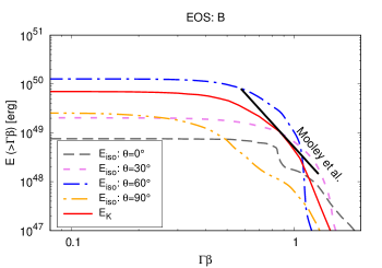
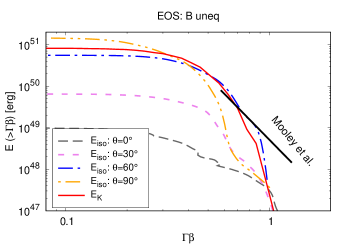
Figure 1: The total kinetic energy and the isotropic equivalent kinetic energy distributions of the dynamical merger ejecta at different polar angles for models B (left) and B uneq (right). Also shown as a solid straight line is the slow quasi-spherical model of Mooley et al. (2018).

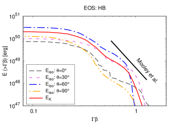
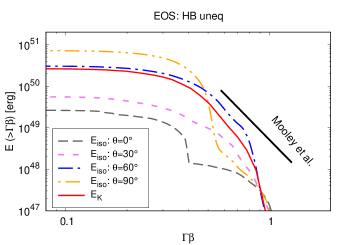
Figure 2: Same as figure 1 but for model HB.

The structure of the paper is as follows: we show in §2 that recent high-resolution numerical relativity simulations reveal such high velocity components and discuss their properties. In §3 we use these profiles to calculate the synchrotron radiation light curves arising from the shock between the ejecta and ISM and compare them with the observed data. Finally, in §4, we discuss the generic features and future expectations of the dynamical ejecta scenario and summarize our conclusions in §5.

2 The fast tail of dynamical ejecta

A small fraction of the dynamical merger ejecta accelerates to mildly relativistic velocities when the shock formed between the colliding neutron stars emerges from the surface (Kyutoku et al., 2014). This component is the high velocity tail of the dynamical ejecta. The flux of the synchrotron radiation arising from the ISM-ejecta shock can be significantly enhanced by even a small amount of a fast ejecta (Piran et al., 2013; Hotokezaka & Piran, 2015). While fast ejecta have been found in previous numerical merger simulations (Hotokezaka et al., 2013; Bauswein et al., 2013; Metzger et al., 2015), its amount was not clear due to the low numerical resolution of those earlier simulations.

We begin by describing the ejecta profile obtained from recent high resolution numerical relativity simulations (Kiuchi et al., 2017), whose the finest grid spacing, $\Delta x$, satisfies: $\Delta x\sim 70$ m. We discuss five models with a total mass of $\approx 2.7M_{\odot}$, a mass ratio of $1$ or $\approx 0.8$, and three different neutron star equations of state: models B, HB, and H (Kiuchi et al., 2017). These models are consistent with the mass and tidal deformability constraints of GW170817 (Abbott et al., 2017). The parameters of these models and the resulting total kinetic energy and mass of the ejecta are listed in Table. 1. Hereafter, we refer to equations of state which give small (large) radius neutron stars as “soft” (“stiff”) equations of state.

Note that, like in practically all other numerical relativistic merger simulations (Hotokezaka et al., 2013; Bauswein et al., 2013; Sekiguchi et al., 2015; Radice et al., 2016; Dietrich et al., 2017; Shibata et al., 2017) in all models the total mass of dynamical ejecta is lower than the one needed to power the observed macronova/kilonova. This additional mass can be driven by other mass ejection mechanisms, such as winds from the surrounding accretion disk or from the hypermassive neutron star that have not been included in these merger simulations (see, e.g., Dessart et al. 2009; Fernández & Metzger 2013; Metzger & Fernández 2014; Perego et al. 2014; Just et al. 2015; Fernández et al. 2015; Fujibayashi et al. 2017; Siegel & Metzger 2017). However, the typical velocity of this wind ejecta is much slower than that of the dynamical ejecta, and hence, this ejecta is not relevant for the early synchrotron emission focused in this paper.

Figures 1 – 3 depict the kinetic energy distributions as a function of $\Gamma\beta$ obtained from the simulations. Here, $\Gamma$ is the Lorentz factor and $\beta$ is the velocity in units of the speed of light. The total kinetic energy of the ejecta is in the range from $\sim 7\cdot 10^{49}$ to $8\cdot 10^{50}$ erg. The ejecta of the softest model B is faster than that of models HB and H. This can be explained if the shock formed at the collision is stronger for more compact neutron stars, and thus, the ejected material is faster. For unequal mass cases the ejecta are predominantly produced through the tidal disruption of the lower mass neutron star and it contains a larger amount of slow material and a smaller amount of fast material compared to the equal mass cases. Note also that the ejecta mass of model B is much smaller than the other models because the merging neutron stars promptly collapse into a black hole, and thus, the mass ejection occurs on only a short time scale.

Table 1: Parameters

Model	$m_{1},\,m_{2}$ [$M_{\odot}$]	$R_{\rm ns}\,[{\rm km}]$	$M_{\rm ej}\,[M_{\odot}]$	$E_{\rm ej}$ [erg]
B	$1.35,\,1.35$	$10.96$	$5\cdot 10^{-4}$	$7\cdot 10^{49}$
HB	$1.35,\,1.35$	$11.61$	$3\cdot 10^{-3}$	$10^{50}$
H	$1.35,\,1.35$	$12.27$	$3\cdot 10^{-3}$	$9\cdot 10^{49}$
B uneq	$1.51,\,1.21$	$10.96$	$10^{-2}$	$8\cdot 10^{50}$
HB uneq	$1.51,\,1.21$	$11.61$	$5\cdot 10^{-3}$	$3\cdot 10^{50}$

$R_{\rm ns}$ is the radius of a non-rotating cold neutron star of $1.35M_{\odot}$.

The isotropic equivalent energy distributions at different polar angles are also shown in Figs. 1 – 3, demonstrating the anisotropy of the ejecta. For the equal mass cases, the material ejected at $30^{\circ}$–$60^{\circ}$ has more kinetic energy. For the unequal mass cases, more material is ejected on the equatorial plane. Another important feature is that the ejecta moving faster than $\Gamma\beta\sim 1$ is somewhat isotropic for all the cases. Therefore, the early light curve arising from this mildly relativistic tail is expected to be rather isotropic.

Also shown in figures 1–3, for a comparison, is the quasi-spherical slow ejecta model used by Mooley et al. (2018):

$$E(>\Gamma\beta)=5\cdot 10^{50}\,{\rm erg\,}(\Gamma\beta/0.4)^{-5}~{}~{}~{}({\rm for}\,\beta<0.8)\ .$$ (1)

This distribution can fit the observed data up to $\sim 100$ days after GW170817. Note that the non-thermal afterglow up to $\sim 100$ days is produced by a component faster than $\beta\approx 0.6$ (Mooley et al., 2018) and, of course, this profile cannot be extended to lower velocities $\beta\ll 0.4$. The total kinetic energy distributions for model B is the closest to this distribution.

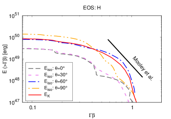
Figure 3: Same as figure 1 but for model H with equal masses.

3 The dynamical ejecta emission

The interaction between the expanding merger ejecta and the surrounding ISM results in a shock, in which particle acceleration and magnetic field amplification occur. As a result, this blast wave emits multi-wavelength synchrotron radiation (Nakar & Piran, 2011). Here, we numerically calculate the synchrotron radiation emitted by the accelerated electrons since we are interested in mildly relativistic blast waves, for which either limits, $\beta\ll 1$, or $\Gamma\gg 1$, cannot be used. To follow the evolution of the ejecta expanding in the ISM with a constant density, $n$, we solve the adiabatic radial expansion of the ejecta at each polar angle using the kinetic energy distributions given in the previous section. The synchrotron flux from the blast wave element at each solid angle at a given observer time is calculated assuming a power-law distribution of electrons, $dN/d\gamma_{e}\propto\gamma_{e}^{-p}$, and the standard equipartition parameters $\epsilon_{e}$ and $\epsilon_{B}$, which reflect the conversion efficiency of the internal energy of the shocked ISM to the accelerated electrons’ energy and magnetic energy respectively (e.g. Sari et al. 1998; Nakar & Piran 2011 and see Hotokezaka & Piran 2015 for details). We fix the viewing angle to be $30^{\circ}$ (Abbott et al., 2017) and set $\epsilon_{e}$ to be $0.1$. Therefore, there are in total three free parameters, $n$, $\epsilon_{B}$, and $p$, with which we fit the observed data in our afterglow modeling.

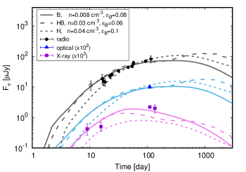
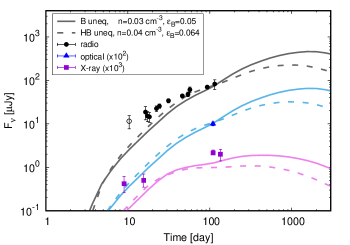
Figure 4: Light curve models of the synchrotron flare that followed GW170817. Left and right panels show the light curves for the equal mass and unequal mass cases, respectively. The solid circles, triangle, and squares show the radio data ($3$ GHz; Hallinan et al. 2017; Mooley et al. 2018; Margutti et al. 2018), optical data (r-band; Margutti et al. 2018; Lyman et al. 2018), and X-ray data (1 keV; Haggard et al. 2017; Troja et al. 2017; Margutti et al. 2017, 2018; Ruan et al. 2017; D’Avanzo et al. 2018; Troja et al. 2018). The optical and X-ray flux densities are multiplied by factor of $10^{2}$ and $10^{3}$ correspondingly. The open circle shows a marginal detection at $6$ GHz (Hallinan et al., 2017) corrected to the flux density at $3$ GHz assuming a spectral index of $-0.55$. The solid, dashed, dotted lines show the theoretical light curve arising from the dynamical merger ejecta for model B, HB, and H, respectively. Here we assume microphysics parameters, $\epsilon_{e}=0.1$ and $p=2.1$, and a viewing angle of $30^{\circ}$.

Figure 4 shows the calculated light curves for the different models as well as the observations of GW170817. The light curves match the observed data, for $n=0.008$–$0.04\,{\rm cm^{-3}}$, $\epsilon_{B}=0.05$–$0.1$, and $p=2.1$. Note that even the higher values of the ISM density are consistent with the upper limit on the mean ISM density of NGC 4993, $n\lesssim 0.04\,{\rm cm^{-3}}$, inferred from the upper limit on the HI mass (Hallinan et al., 2017). For the equal mass cases, the radio and optical light curves continuously rise up to $\sim 100$ days and then have a plateau phase lasting a few hundred days. This early component is produced by the tail of the ejecta faster than $\Gamma\beta\sim 0.6$. Model H contains a lower kinetic energy at $\Gamma\beta\sim 1$. As this fastest component dominates the early light curve the flux density up to $20$ days is lower than those of model B and HB.

For unequal masses, the flux densities continuously rise until $1000$ days because of the larger amount of material at low velocities. However, the slope of the calculated light curves is steeper than the observed one because the kinetic energy distribution of the these models declines more steeply at high velocities.

An important feature of the X-ray light curves is that they peak on a time scale of a few months to a year and then their temporal evolution is different from that of the radio and optical light curves once the synchrotron cooling frequency becomes lower than $1$ keV. For model H, in particular, the cooling frequency falls below 1 keV at early times $\sim 10$ days because of the required relatively large values of the ISM density and $\epsilon_{B}$. Note that the exact location of the cooling frequency can be higher due to several uncertainties (see the discussion in the next section). However, it is generally expected that the cooling frequency crosses the X-ray band on a time scale of a few months to a year in this scenario.

4 Discussion

Cooling frequency: An important feature of the synchrotron light curves obtained in §3 is the evolution of the synchrotron cooling frequency, that crosses the X-ray band on a time scale of a few months to a year. After this time, the X-ray flux density declines with time faster than the radio and optical flux densities. In the Newtonian limit ($\beta\ll 1$), the cooling frequency at a given time, $t$, is approximately estimated as (e.g., Sari et al. 1998)

$$\nu_{c} \sim 0.5\,{\rm keV}\left(\frac{\beta}{0.6}\right)^{-3}\left(\frac{n}{0.01\,{\rm cm^{-3}}}\right)^{-3/2}$$

$$~{}~{}~{}~{}~{}~{}~{}~{}~{}~{}~{}~{}~{}~{}\times\left(\frac{\epsilon_{B}}{0.05}\right)^{-3/2}\left(\frac{t}{100\,{\rm days}}\right)^{-2},$$

or the cooling frequency for a given flux density is

$$\nu_{c}\propto\beta^{\frac{5p-6}{3}}n^{\frac{p-4}{6}}\epsilon_{B}^{\frac{p-8}{6}}\epsilon_{e}^{\frac{2(p+1)}{3}}F_{\nu}^{-\frac{2}{3}},$$ (3)

where $F_{\nu}$ is the flux density at a frequency in the range of $\nu_{a},\,\nu_{m}<\nu<\nu_{c}$. Note that, for a given flux density, the cooling frequency increases by decreasing $n$ and $\epsilon_{B}$ and by increasing the velocity for the expected range of the electrons’ power-law index, $2<p<3$. In other words, it depends sensitively on the kinetic energy of the fast tail. The cooling frequency can be higher than those of our models if the kinetic energy at velocities faster than $\beta\sim 0.6$ is only slightly larger. For instance, the kinetic energy distribution of Eq. (1) results in $\nu_{c}\gtrsim 10$ keV at $100$ days (Mooley et al., 2018). Note also that the cooling frequency is much higher for the cocoon models (Mooley et al., 2018; Nakar & Piran, 2018; Margutti et al., 2018; Lyman et al., 2018), that involve an outflow much faster than the fast tail of the dynamical ejecta (see, e.g., Gottlieb et al., 2017; Lazzati et al., 2017; Nakar & Piran, 2018).

The X-ray observations around $100$ days show that the X-ray flux density and the photon index in the X-ray band are consistent with a single power-law spectrum from the radio to the X-ray bands (Mooley et al., 2018; Margutti et al., 2018; Ruan et al., 2017; D’Avanzo et al., 2018; Troja et al., 2018). This suggests that the cooling frequency is above the X-ray band, ruling out models with much lower cooling frequency, e.g., model H. However, it should be noted that the estimate of equation (4) and the cooling frequency used in our light curve modeling are correct only within an order of magnitude. In fact, Granot & Sari (2002) obtained the spectral breaks of the afterglows for the Blandford-McKee solution and found that the cooling frequency was higher by a factor of $\gtrsim 3$ than the simple order of magnitude estimate (Sari et al., 1998). Therefore, models B and HB for the equal mass caes can be considered as consistent with the current observed data. However, a generic expectation of the dynamical ejecta scenario is that the cooling frequency will cross the X-ray band on a time scale not much longer than a few months. Therefore further multi-frequency observations will easily confirm or rule out this model.

Late-time signal: In addition to the fast moving dynamical ejecta, there should be a main, sub-relativistic ejecta component that have produced the uv/optical/IR macronova/kilonova signal. As already mentioned the dynamical ejecta masses of our models, $5\cdot 10^{-4}$–$10^{-2}M_{\odot}$, are much smaller than those estimated from the macronova observations, $\sim 0.05M_{\odot}$ (e.g., Kasliwal et al. 2017). This component has the photospheric velocities of $\sim 0.1$–$0.3c$ and a kinetic energy of $\sim 10^{51}$ erg, which is also larger than the kinetic energy of the dynamical ejecta in our dynamical ejecta models. Some other processes, not taken into account in the simulations used in this work, must be responsible for the ejection of this additional mass.

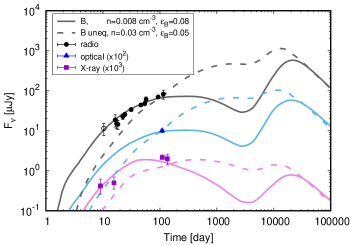
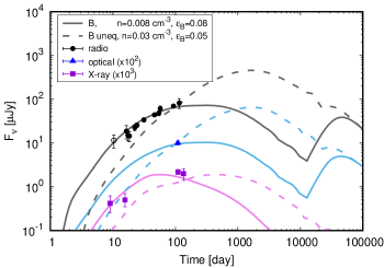
Figure 5: Same as figure 4 but on a longer time scale. The radio flare arising from the ejecta component that produced the uv/optical/nIR macronova signal is also shown. For this component, we assume a mass of $0.04M_{\odot}$ and a single velocity of $0.2c$ (top) and $0.1c$ (bottom), and the ISM density and microphysics parameters are the same to the dynamical ejecta component of each model.

Considering now the total ejected mass as observed from the uv/optical/IR macronova, we estimate the peak time and flux density of this slow component (Nakar & Piran, 2011):

$$t_{\rm p} \approx 10^{4}\,{\rm day}\,\left(\frac{E}{10^{51}\,{\rm erg}}\right)^{\frac{1}{3}}\left(\frac{n}{0.01\,{\rm cm^{-3}}}\right)^{-\frac{1}{3}}\left(\frac{\beta}{0.2}\right)^{-\frac{5}{3}},$$ (4)

$$F_{\nu,{\rm p}} \approx 2\,{\rm mJy}\,\epsilon_{B,-1}^{0.775}\epsilon_{e,-1}^{1.1}\left(\frac{E}{10^{51}\,{\rm erg}}\right)$$

$$~{}~{}~{}~{}~{}~{}\times\left(\frac{n}{0.01\,{\rm cm^{-3}}}\right)^{0.775}\left(\frac{\beta}{0.2}\right)^{1.75}\left(\frac{\nu}{3\,{\rm GHz}}\right)^{-0.55},$$

where $\epsilon_{B,-1}$ and $\epsilon_{e,-1}$ are normalized by $0.1$ and we set $p=2.1$. Figure 5 depicts the flux densities from the dynamical ejecta and the macronova ejecta. Here we assume that the macronova ejecta has a mass of $0.04M_{\odot}$ and a single velocity of $0.2c$ (top panel) and $0.1c$ (bottom panel), and set the ISM density and the same microphysics parameters as those used for the dynamical ejecta models (see figure 4). The bumps around $10^{4}$ –$10^{5}$ days in the light curves are produced by the macronova component. The actual shape of the peak of the light curves is expected to be broader due to the velocity structure of the macronova ejecta. Note that the cooling frequency of the late emission is around the uv/optical bands so that the estimate of equation (4) is applicable up to the optical band and the X-ray flux density of the macronova component is much fainter than that estimated by equation (4).

This late-time emission is one of the notable differences between the dynamical ejecta and cocoon/structure jet scenarios. For the cocoon/structure jet scenario, in which the ISM density is much lower than that of the dynamical ejecta scenario, the flux density from the macronova ejecta is expected to be much fainter $\lesssim 50\,{\rm\mu Jy}$ and the peak time is much longer, $\gtrsim 100$ yr.

Angular size: The velocity of the fast tail that produces the afterglow at $100$ days is $\sim 0.6c$. Therefore, the angular size of the afterglow is $\lesssim 500\,{\rm\mu arcsec}(t/100\,{\rm day})$ for $>100$ days. This is smaller by a factor a few compared to that expected in the cocoon and structured jet models. Therefore, these scenarios can be distinguished by future VLBI observations (Hallinan et al. 2017).

5 Conclusion

The fast tail ($\Gamma\beta\sim 1$) of the dynamical ejecta of binary neutron star mergers, calculated in recent high resolution numerical simulations by Kiuchi et al. (2017) contains kinetic energy of $10^{47}$ – $10^{49}$ erg, depending on the neutron star equation of state and on the binary masses. Mergers with a softer neutron star equation of state, which gives smaller radius neutron stars, and with a mass ratio close to unity eject larger amounts of the fast tail. The fast tail has somewhat isotropic shape even for models in which the bulk of the material is large aspherical.

The interaction of this fast tail with the surrounding ISM produces a blast wave whose synchrotron emission (Nakar & Piran, 2011) is observed as the radio to X-ray signals that followed GW170817. We compute this synchrotron emission arising from the ejecta profile obtained from the high resolution numerical relativity simulations and compare them with the observed data of the non-thermal radiation that followed GW170817. We find that the multi-frequency observed data can be reproduced well for the equal mass binary models with a relatively soft equation of state. In all cases, an ISM density of $\sim 0.01\,{\rm cm^{-3}}$ is required to obtain the observed flux level at $\sim 100$ days after the merger. For unequal mass cases, the velocity gradient of the ejecta profile is steeper and the light curves rise more steeply than the observed one so that nearly equal mass mergers are favored in this scenario.

The dynamical ejecta scenario has three generic predictions:

1. The cooling frequency crosses the X-ray band on a time scale of a few months to a year leading to a cooling break in the X-ray light curve.

2. The outer ejecta velocity is $\lesssim 0.6c$ at $t\gtrsim 100$ days so that the angular size of the ejecta will be $\lesssim 500\,\mu{\rm arcsec}(t/100\,{\rm day})$.

3. The emission of the sub-relativistic macronova/kilonova component of a mass of $\sim 0.05M_{\odot}$ and a velocity of $\sim 0.1c$ will be continuously observable with flux densities of $0.1$–$1$ mJy on time scales of $10^{3}$ – $10^{5}$ days (Nakar & Piran, 2011; Piran et al., 2013; Hotokezaka & Piran, 2015).

These features will enable us to observationally confirm or rule out this model in the near future.

References

- Abbott et al. (2017) Abbott, B. P., et al. 2017, Phys. Rev. Lett., 119, 161101
- Abbott et al. (2017) Abbott, B. P., Abbott, R., Abbott, T. D., et al. 2017, ApJ, 848, L12
- Andreoni et al. (2017) Andreoni, I., et al. 2017, Submitted to: Publ. Astron. Soc. Austral., arXiv:1710.05846
- Arcavi et al. (2017) Arcavi, I., Hosseinzadeh, G., Howell, D. A., et al. 2017, Nature, 551, 64
- Bauswein et al. (2013) Bauswein, A., Goriely, S., & Janka, H.-T. 2013, ApJ, 773, 78
- Côté et al. (2017) Côté, B., Fryer, C. L., Belczynski, K., et al. 2017, ArXiv e-prints, arXiv:1710.05875
- Coulter et al. (2017) Coulter, D. A., Foley, R. J., Kilpatrick, C. D., et al. 2017, Science, 358, 1556
- Cowperthwaite et al. (2017) Cowperthwaite, P. S., et al. 2017, Astrophys. J., 848, L17
- D’Avanzo et al. (2018) D’Avanzo, P., Campana, S., Ghisellini, G., et al. 2018, ArXiv e-prints, arXiv:1801.06164
- Dessart et al. (2009) Dessart, L., Ott, C. D., Burrows, A., Rosswog, S., & Livne, E. 2009, ApJ, 690, 1681
- Dietrich et al. (2017) Dietrich, T., Ujevic, M., Tichy, W., Bernuzzi, S., & Brügmann, B. 2017, Phys. Rev. D, 95, 024029
- Drout et al. (2017) Drout, M. R., Piro, A. L., Shappee, B. J., et al. 2017, Science, 358, 1570
- Eichler et al. (1989) Eichler, D., Livio, M., Piran, T., & Schramm, D. N. 1989, Nature, 340, 126
- Evans et al. (2017) Evans, P. A., Cenko, S. B., Kennea, J. A., et al. 2017, Science, 358, 1565
- Fernández & Metzger (2013) Fernández, R., & Metzger, B. D. 2013, MNRAS, 435, 502
- Fernández et al. (2015) Fernández, R., Quataert, E., Schwab, J., Kasen, D., & Rosswog, S. 2015, MNRAS, 449, 390
- Fujibayashi et al. (2017) Fujibayashi, S., Kiuchi, K., Nishimura, N., Sekiguchi, Y., & Shibata, M. 2017, ArXiv e-prints, arXiv:1711.02093
- Gottlieb et al. (2018) Gottlieb, O., Nakar, E., & Piran, T. 2018, MNRAS, 473, 576
- Gottlieb et al. (2017) Gottlieb, O., Nakar, E., Piran, T., & Hotokezaka, K. 2017, ArXiv e-prints, arXiv:1710.05896
- Granot & Sari (2002) Granot, J., & Sari, R. 2002, ApJ, 568, 820
- Haggard et al. (2017) Haggard, D., Nynka, M., Ruan, J. J., et al. 2017, Astrophys. J., 848, L25
- Hallinan et al. (2017) Hallinan, G., Corsi, A., Mooley, K. P., et al. 2017, Science, 358, 1579
- Hotokezaka et al. (2018) Hotokezaka, K., Beniamini, P., & Piran, T. 2018, ArXiv e-prints, arXiv:1801.01141
- Hotokezaka et al. (2013) Hotokezaka, K., Kiuchi, K., Kyutoku, K., et al. 2013, Phys. Rev. D, 87, 024001
- Hotokezaka & Piran (2015) Hotokezaka, K., & Piran, T. 2015, MNRAS, 450, 1430
- Just et al. (2015) Just, O., Bauswein, A., Pulpillo, R. A., Goriely, S., & Janka, H.-T. 2015, MNRAS, 448, 541
- Kasen et al. (2017) Kasen, D., Metzger, B., Barnes, J., Quataert, E., & Ramirez-Ruiz, E. 2017, Nature, 551, 80
- Kasliwal et al. (2017) Kasliwal, M. M., Nakar, E., Singer, L. P., et al. 2017, Science, 358, 1559
- Kilpatrick et al. (2017) Kilpatrick, C. D., et al. 2017, arXiv:1710.05434
- Kiuchi et al. (2017) Kiuchi, K., Kawaguchi, K., Kyutoku, K., et al. 2017, Phys. Rev. D, 96, 084060
- Kyutoku et al. (2014) Kyutoku, K., Ioka, K., & Shibata, M. 2014, MNRAS, 437, L6
- Lattimer & Schramm (1974) Lattimer, J. M., & Schramm, D. N. 1974, ApJ, 192, L145
- Lazzati et al. (2017) Lazzati, D., Perna, R., Morsony, B. J., et al. 2017, ArXiv e-prints, arXiv:1712.03237
- Lipunov et al. (2017) Lipunov, V. M., Gorbovskoy, E., Kornilov, V. G., et al. 2017, ApJ, 850, L1
- Lyman et al. (2018) Lyman, J. D., Lamb, G. P., Levan, A. J., et al. 2018, ArXiv e-prints, arXiv:1801.02669
- Margutti et al. (2017) Margutti, R., Berger, E., Fong, W., et al. 2017, ApJ, 848, L20
- Margutti et al. (2018) Margutti, R., Alexander, K. D., Xie, X., et al. 2018, ArXiv e-prints, arXiv:1801.03531
- Metzger et al. (2018) Metzger, B. D., Thompson, T. A., & Quataert, E. 2018, ArXiv e-prints, arXiv:1801.04286
- Metzger et al. (2015) Metzger, B. D., Bauswein, A., Goriely, S., & Kasen, D. 2015, MNRAS, 446, 1115
- Metzger & Fernández (2014) Metzger, B. D., & Fernández, R. 2014, MNRAS, 441, 3444
- Mooley et al. (2018) Mooley, K. P., Nakar, E., Hotokezaka, K., et al. 2018, Nature, 554, 207
- Nakar & Piran (2011) Nakar, E., & Piran, T. 2011, Nature, 478, 82
- Nakar & Piran (2018) —. 2018, ArXiv e-prints, arXiv:1801.09712
- Perego et al. (2017) Perego, A., Radice, D., & Bernuzzi, S. 2017, ApJ, 850, L37
- Perego et al. (2014) Perego, A., Rosswog, S., Cabezón, R. M., et al. 2014, MNRAS, 443, 3134
- Pian et al. (2017) Pian, E., D’Avanzo, P., Benetti, S., et al. 2017, Nature, 551, 67
- Piran et al. (2013) Piran, T., Nakar, E., & Rosswog, S. 2013, MNRAS, 430, 2121
- Radice et al. (2016) Radice, D., Galeazzi, F., Lippuner, J., et al. 2016, MNRAS, 460, 3255
- Rosswog et al. (2017) Rosswog, S., Sollerman, J., Feindt, U., et al. 2017, ArXiv e-prints, arXiv:1710.05445
- Ruan et al. (2017) Ruan, J. J., Nynka, M., Haggard, D., Kalogera, V., & Evans, P. 2017, ArXiv e-prints, arXiv:1712.02809
- Sari et al. (1998) Sari, R., Piran, T., & Narayan, R. 1998, ApJ, 497, L17+
- Sekiguchi et al. (2015) Sekiguchi, Y., Kiuchi, K., Kyutoku, K., & Shibata, M. 2015, Phys. Rev. D, 91, 064059
- Shibata et al. (2017) Shibata, M., Fujibayashi, S., Hotokezaka, K., et al. 2017, Phys. Rev. D, 96, 123012
- Siegel & Metzger (2017) Siegel, D. M., & Metzger, B. D. 2017, ArXiv e-prints, arXiv:1705.05473
- Smartt et al. (2017) Smartt, S. J., Chen, T.-W., Jerkstrand, A., et al. 2017, Nature, 551, 75
- Tanaka et al. (2017) Tanaka, M., et al. 2017, Publ. Astron. Soc. Jap., arXiv:1710.05850
- Tanvir et al. (2017) Tanvir, N. R., et al. 2017, Astrophys. J., 848, L27
- Troja et al. (2017) Troja, E., Piro, L., van Eerten, H., et al. 2017, Nature, 551, 71
- Troja et al. (2018) Troja, E., Piro, L., Ryan, G., et al. 2018, ArXiv e-prints, arXiv:1801.06516
- Utsumi et al. (2017) Utsumi, Y., et al. 2017, Publ. Astron. Soc. Japan, arXiv:1710.05848
- Valenti et al. (2017) Valenti, S., Sand, D. J., Yang, S., et al. 2017, Astrophys. J., 848, L24
- Villar et al. (2017) Villar, V. A., Guillochon, J., Berger, E., et al. 2017, ApJ, 851, L21
- Waxman et al. (2017) Waxman, E., Ofek, E., Kushnir, D., & Gal-Yam, A. 2017, ArXiv e-prints, arXiv:1711.09638