Black Hole-Neutron Star Binaries in General Relativity: Quasiequilibrium Formulation

Abstract

We present a new numerical method for the construction of quasiequilibrium models of black hole-neutron star binaries. We solve the constraint equations of general relativity, decomposed in the conformal thin-sandwich formalism, together with the Euler equation for the neutron star matter. We take the system to be stationary in a corotating frame and thereby assume the presence of a helical Killing vector. We solve these coupled equations in the background metric of a Kerr-Schild black hole, which accounts for the neutron star’s black hole companion. In this paper we adopt a polytropic equation of state for the neutron star matter and assume large black hole–to–neutron star mass ratios. These simplifications allow us to focus on the construction of quasiequilibrium neutron star models in the presence of strong-field, black hole companions. We summarize the results of several code tests, compare with Newtonian models, and locate the onset of tidal disruption in a fully relativistic framework.

I Introduction

Black hole-neutron star (hereafter BHNS) binaries have attracted considerable astrophysical interest recently. For example, they are candidates for the central engines of short-period, gamma-ray bursts jerf99 . They are also very promising sources of gravitational radiation for the new generation of ground-based gravitational wave detectors, including the Laser Interferometer Gravitational Wave Observatory (LIGO), and the future space-based gravitational wave detector, the Laser Interferometer Space Antenna (LISA). Observation of a BHNS binary – in particular, the tidal disruption of a neutron star by a black hole companion – will provide spectacular information on the gravitational fields in relativistic objects and the nuclear physics governing neutron star matter (e.g. v00 ). However, BHNS binaries may be among the most challenging objects in relativistic astrophysics to model numerically. Any realistic treatment must deal simultaneously with the difficulties associated with the spacetime singularity inside the black hole and the complexities associated with relativistic hydrodynamics.

The inspiral of BHNS binaries is driven by the emission of gravitational radiation, which extracts both energy and angular momentum from the binary and also tends to circularize the orbit. As long as the binary separation is large, the inspiral is very slow and radial velocities are very small compared to the orbital velocities once the orbit has been circularized. During this phase, the inspiral can be modeled as a sequence of quasicircular binary orbits. The quasiadiabatic inspiral phase ends when dynamical effects become important. For BHNS binaries, there are at least two, very different, possible termination points: the binary may reach an innermost stable circular orbit (ISCO), at which point the orbit becomes unstable and the black hole and neutron star plunge rapidly towards each other, or, prior to reaching the ISCO, the neutron star might be tidally distrupted by the gravitational field of the black hole. Predicting which one of these scenarios actually happens, and the binary separation at which it occurs, depends on a number of factors characterizing the system, including the binary mass ratio.

The importance of tidal effects can be estimated, in a Newtonian framework, by comparing the tidal force on a test mass $m$ on the surface of the neutron star

$$F_{\rm tid}\sim G\frac{mM_{\rm BH}R_{\rm NS}}{s^{3}},$$ (1)

with the gravitational force exerted by the star

$$F_{\rm grav}\sim G\frac{mM_{\rm NS}}{R_{\rm NS}^{2}}.$$ (2)

Here $M_{\rm BH}$ and $M_{\rm NS}$ are the masses of the black hole and the neutron star, $R_{\rm NS}$, is the neutron star radius and $s$ is the binary separation. Equating the two forces yields an approximate critical “tidal” separation

$$\frac{s_{\rm tid}}{R_{\rm NS}}\sim\left(\frac{M_{\rm BH}}{M_{\rm NS}}\right)^{1/3},$$ (3)

or, in gravitational units with $G=c=1$,

$$\frac{s_{\rm tid}}{M_{\rm BH}}\sim\left(\frac{M_{\rm NS}}{M_{\rm BH}}\right)^{2/3}\frac{R_{\rm NS}}{M_{\rm NS}},$$ (4)

within which tidal forces begin to dominate and may lead to tidal disruption.

Neutron stars typically have compaction ratios of $R_{\rm NS}/M_{\rm NS}\sim 5$. That means that for neutron stars orbiting supermassive black holes, $M_{\rm BH}\gg M_{\rm NS}$, so that the tidal separation is well inside the ISCO, which resides at about $s\sim 6M_{\rm BH}$ (the value for a point-mass orbiting a Schwarzschild black hole). It is therefore appropriate to neglect any effects of tidal distortion or internal structure in calculations of neutron stars inspiral onto supermassive black holes. Such binaries may be a promising sources of low-frequency gravitational radiation for detection by LISA.

For neutron stars orbiting stellar mass black holes, however, the internal structure of the neutron star may become important before it reaches the ISCO. Such objects may be important high-frequency sources for LIGO and other ground based gravitational wave detectors. Any future detection of such inspiraling binaries may therefore carry information about the internal structure of the neutron star and its equation of state v00 .

Considerable effort has gone into the theoretical modeling of binaries containing either two black holes (e.g. c94 ; b00 ; ggb02 ) or two neutron stars (e.g. wm95 ; bcsst ; use00 ; ggtmb01 ; tg02 ; see also the reviews bs03 ; c00 ). For the most part, BHNS binaries have been studied only in Newtonian gravity (but see m01 ). Several authors lrs93 ; tn96 have modeled BHNS binaries as Newtonian ellipsoids around point masses, generalizing the classic Roche model for incompressible stars (see, e.g.  ch69 ) to compressible configurations. These ellipsoidal calculations have also been generalized to include relativistic effects f73 ; s96 ; wl00 . Equilibrium models of Newtonian BHNS binaries also have been constructed by solving the exact fluid equations numerically and again treating the black hole as a point mass ue99 . Dynamical simulations of Newtonian BHNS binaries, including coalescence, merger, and the tidal disruption of the neutron star, have been performed, for example, by (jerf99, ; l01, , and references therein). Dynamical simulations have also been performed for the tidal disruption of normal stars orbiting massive black holes (see, e.g. kl04 and references therein). But, at best, these simulations typically employ a relativistic treatment of the hydrodynamics with an approximate treatment of the gravitational field of the star and/or the gravitational tidal field of the black hole companion. There is greater urgency in solving this problem more carefully, now that the possible detections by the Chandra X-ray Observatory of tidal disruptions of normal stars by supermassive black holes have been reported hg04 . Clearly, accurate and reliable models of binaries containing black holes, including BHNS binaries, require a fully relativistic treatment.

This paper is the first in a series on quasiequilibrium models of BHNS binaries in full general relativity. Our models serve a dual purpose: (1) constant rest-mass, quasiequilibrium sequences parametrized by binary separation approximate the adiabatic inspiral phase and can be used to locate the ISCO or the onset of tidal instability, and (2) individual models provide numerically exact initial data for future relativistic dynamical simulations. Similar to earlier treatments of binary neutron stars (e.g. wm95 ; bcsst ; use00 ; ggtmb01 ; tg02 ) and binary black holes (e.g. ggb02 ), we adopt the conformal thin-sandwich decomposition y99 of the constraint equations of general relativity. We solve these equations for the gravitational field, together with the relativistic Euler equation for the matter, assuming the presence of a helical Killing vector. For the background geometry, we adopt the metric corresponding to a single black hole in Kerr-Schild coordinates, thereby accounting for the black hole companion of the neutron star.

In this first paper we provide solutions for the simplest case in which the mass ratio is large, i.e., $M_{\rm BH}\gg M_{\rm NS}$. While the estimate above shows that, in this limit, the internal structure of the neutron star and tidal distortion is small, it allows us to formulate the BHNS problem in full general relativity and to construct numerical models of a neutron star in the presence of a black hole companion. We also adopt a polytropic equation of state for the neutron star matter. In a future paper we will relax these approximations and will construct binaries with companions of comparable mass, for which the internal struture, tidal distortion and tidal disruption are potentially very important.

The paper is structured as follows. In Section II we describe how the BHNS problem can be solved in Newtonian gravity. A very similar approach is adopted in the relativistic treatment, so it is useful to outline this approach first in the much more transparent Newtonian framework. In Section III we develop the relativistic formalism. We introduce the assumption of extreme mass ratios in Section IV. In Section V we present numerical results, including code tests and constant rest-mass sequences. We provide a brief summary in Section VI. A detailed description of the numerical strategy that we adopted in solving the relativistic equations, together with Kerr-Schild background expressions that appear in these equations, can be found in Appendix A. Throughout this paper we continue to adopt geometrized units ($G=c=1$).

II BHNS Binaries in Newtonian Gravity

Before turning to the relativistic problem, it is useful to lay out in this Section how BHNS binaries can be constructed in the much simpler Newtonian framework (compare ue99 ). In the Sections that follow we will adopt a very similar strategy and algorithm for the construction of the same binaries in general relativity, and will refer back to this Section for clarity.

II.1 The Poisson Equation

In Newtonian gravity, the black hole can be described by a point mass $M_{\rm BH}$ which gives rise to the gravitational potential

$$\phi_{\rm BH}=-\frac{M_{\rm BH}}{r_{\rm BH}},$$ (5)

where $r_{\rm BH}$ is the distance from the point mass. The total gravitational field $\phi$ can be written as a sum

$$\phi=\phi_{\rm BH}+\phi_{\rm NS},$$ (6)

where $\phi_{\rm NS}$ is the neutron star contribution to the potential. Since $\phi_{\rm BH}$ is a homogeneous solution to the Poisson equation (for $r_{\rm BH}>0$), we can write the Poisson equation as

$$D^{2}\phi=D^{2}\phi_{\rm NS}=4\pi\rho_{0}$$ (7)

where $D^{2}$ is the Laplace operator.

II.2 The Integrated Euler Equation

Figure 1: Coordinate system that we use for the construction of BHNS binaries. The origin is centered on the neutron star, the black hole is located at the position $x_{\rm BH}$, and the axis of rotation, which is parallel to the $z$-axis, is located at $x_{\rm rot}$. For the extreme mass ratio $M_{\rm BH}\gg M_{\rm NS}$ adopted in this paper we have $x_{\rm BH}=x_{\rm rot}$.

We assume a polytropic equation of state

$$P=\kappa\rho_{0}^{1+1/n},$$ (8)

where $P$ is the pressure, $\rho_{0}$ the (rest-mass) density, $n$ the polytropic index and $\kappa$ the polytropic constant. For corotating equilibrium configurations the Euler equations can then be integrated analytically to yield

$$(n+1)\frac{P}{\rho_{0}}+\phi-\frac{1}{2}\Omega^{2}\left((x-x_{\rm rot})^{2}+y^{2}\right)=C,$$ (9)

where $\Omega$ is the orbital angular velocity, $C$ is a constant and where we have assumed that the star orbits about an axis parallel to the $z$-axis located at $x=x_{\rm rot}$ and $y=0$. In the following we will also assume that the black hole and neutron star are aligned with the $x$-axis (see Fig. 1).

We point out that it is unlikely that the neutron star viscosity could be strong enough to lock the star into corotation during the binary inspiral bc92 ; visc_fn . Therefore it would be more realistic astrophysically to assume an irrotational rather than a corotational fluid flow (see, e.g., bs03 and references therein). However, the numerical implementation of irrotational fluid flow is much more involved than that of corotation, and it is therefore reasonable to focus on corotating configurations first (as it was done for binary neutron stars).

Equations (7) and (9) are the fundamental equations describing a stationary star orbiting a black hole in circular co-rotation. The solution will depend on three parameters, which can be chosen, for example, to be the neutron star mass

$$M_{\rm NS}=\int\rho_{0}d^{3}x,$$ (10)

the black hole mass $M_{\rm BH}$ and the separation $d$. For computational reasons we will use the maximum density of the neutron star as one of the three free parameters instead of the neutron star mass. Given these parameters, a solution to the problem will also provide the eigenvalues $\Omega$ and $C$, as well as the size of the neutron star.

II.3 Elimination of Dimensions

It is convenient to introduce the dimensionless density parameter

$$q=\frac{P}{\rho_{0}},$$ (11)

in terms of which we have

$$\rho_{0}=\kappa^{-n}q^{n}$$ (12)

and

$$P=\kappa^{-n}q^{n+1}.$$ (13)

Since $\kappa^{n/2}$ has units of length, we can also introduce dimensionless coordinates $\bar{x}=\kappa^{-n/2}x$, and similarly for $y$ and $z$. The Laplace operator then scales as $\bar{D}^{2}=\kappa^{n}D^{2}$, and the angular velocity as $\bar{\Omega}=\kappa^{n/2}\Omega$. In terms of these, equations (7) and (9) become

$$\bar{D}^{2}\phi_{\rm NS}=4\pi q^{n}$$ (14)

and

$$(n+1)q+\phi-\frac{1}{2}\bar{\Omega}^{2}\left((\bar{x}-\bar{x}_{\rm rot})^{2}+\bar{y}^{2}\right)=C.$$ (15)

The integrated Euler equation (15) can also be rewritten as

$$q = \frac{1}{n+1}\left(C-\phi+\frac{1}{2}\bar{\Omega}^{2}\left((\bar{x}-\bar{x}_{\rm rot})^{2}+\bar{y}^{2}\right)\right)$$ (16)

$$= \frac{1}{n+1}\left(C-\Phi_{\rm eff}\right),$$

where the effective potential $\Phi_{\rm eff}$ combines the gravitational and centrifugal potentials,

$$\Phi_{\rm eff}=\phi-\frac{1}{2}\bar{\Omega}^{2}\left((\bar{x}-\bar{x}_{\rm rot})^{2}+\bar{y}^{2}\right).$$ (17)

This demonstrates that, up to a constant, the density parameter $q$ is proportional to the effective potential.

Rescaling $\bar{M}=\kappa^{-n/2}M$ we also find

$$\bar{M}_{\rm NS}=\int q^{n}d^{3}\bar{x}.$$ (18)

II.4 Rescaling

As we will see below, it is convenient for numerical purposes to have the surface of the neutron star intersect the $x$-axis at fixed coordinate locations, say $\hat{x}_{A}=-1$ and $\hat{x}_{B}=1$. This means that we have to rescale the coordinates with respect to the physical, non-dimensional size of the neutron star, say $\bar{r}_{e}$. For spherical stars, $\bar{r}_{e}$ is the radius of the star, and otherwise it is half the star’s diameter along the $x$-axis. We denote these new coordinates with hatted quantities, $\hat{x}=\bar{x}/\bar{r}_{e}$, and similarly for $y$ and $z$. The derivative operator scales according to $\hat{D}_{i}=\bar{r}_{e}\bar{D}_{i}$, and we also have $\hat{\Omega}=\bar{r}_{e}\bar{\Omega}$. The Poisson equation (14) then becomes

$$\hat{D}^{2}\phi_{\rm NS}=4\pi\bar{r}_{e}^{2}q^{n}$$ (19)

and the integrated Euler equation (15)

$$(n+1)q+\phi-\frac{1}{2}\hat{\Omega}^{2}\left((\hat{x}-\hat{x}_{\rm rot})^{2}+\hat{y}^{2}\right)=C.$$ (20)

In these coordinates, the physical, dimensionless neutron star mass $\bar{M}_{\rm NS}$ can be computed from

$$\bar{M}_{\rm NS}=\int q^{n}d^{3}\bar{x}=\bar{r}_{e}^{3}\int q^{n}d^{3}\hat{x}.$$ (21)

From the Poisson equation (19) it is evident that the gravitational potential $\phi$ will depend on $\bar{r}_{e}$. To make this dependence explicit, we could introduce a rescaled potential

$$\phi_{\rm NS}=\bar{r}_{e}^{2}\hat{\phi}_{\rm NS}.$$ (22)

This expression can then be inserted into (20), explicitly introducing $\bar{r}_{e}$ into the integrated Euler equation. We have yet to determine the scaling of the black hole contribution $\phi_{\rm BH}$

$$\phi_{\rm BH}=\frac{M_{\rm BH}}{r_{\rm BH}}=\frac{\bar{M}_{\rm BH}}{\bar{r}_{\rm BH}}=\frac{1}{\bar{r}_{e}}\,\frac{\bar{M}_{\rm BH}}{\hat{r}_{\rm BH}}.$$ (23)

Here $\bar{M}_{\rm BH}$ is the dimensionless black hole mass that we want to keep fixed during the iteration.

With these choices, the integrated Euler equation (20) can now be rewritten as

$$(n+1)q+\phi_{\rm NS}-\frac{\bar{M}_{\rm BH}}{\bar{r}_{e}\hat{r}_{\rm BH}}-\frac{1}{2}\hat{\Omega}^{2}\left((\hat{x}-\hat{x}_{\rm rot})^{2}+\hat{y}^{2}\right)=C.$$ (24)

This equation has to be solved together with the Poisson equation (19). A self-consistent solution can be constructed iteratively, as outlined immediately below.

II.5 Iteration Scheme

Instead of fixing the neutron star mass, we fix the maximum density on the $x$-axis $q_{\rm max}$. A neutron star of a desired mass can later be constructed iteratively by varying $q_{\rm max}$. We also fix the separation $x_{\rm BH}$ in terms of the neutron star size $\bar{r}_{e}$, $\hat{x}_{\rm BH}=\bar{x}_{\rm BH}/\bar{r}_{e}$. In the following we will locate the point mass at $(-\hat{x}_{\rm BH},0,0)$. The three input parameters are therefore $q_{\rm max}$, $\hat{x}_{\rm BH}$ and $\bar{M}_{\rm BH}$.

In this paper we also assume that the mass of the black hole is much greater than that of the neutron star

$$\bar{M}_{\rm BH}\gg\bar{M}_{\rm NS},$$ (25)

in which case the rotation axis will go through the center of the black hole

$$\hat{x}_{\rm rot}=\hat{x}_{\rm BH}.$$ (26)

This assumption leads to an error in the location of the rotation axis of the order of $M_{\rm NS}/M_{\rm BH}$ times the binary separation; this becomes negligible as the mass ratio decreases. Without this assumption, the location of the rotation axis $\hat{x}_{\rm rot}$ has to be found as part as the iteration scheme. Various approaches can be chosen to identify $\hat{x}_{\rm rot}$; in Newtonian theory it coincides with the center of mass.

In the limit of extreme mass ratios we expect that the neutron star will affect the physical solution only in a neighborhood of the star itself, so that we can confine the numerical grid to a finite domain around the neutron star that avoids the black hole. This significantly simplifies the problem, especially in the relativistic case, where the black hole interior does not have to be excised from the numerical grid.

The iteration scheme starts with an initial guess for the density $q$, confined between $\hat{x}_{A}$ and $\hat{x}_{B}$, and the star’s physical size $\bar{r}_{e}$.

II.5.1 Solution of the Poisson equation

Given a density distribution $q$ we can solve the Poisson equation (19) to find the neutron star potential $\phi_{\rm NS}$. The elliptic equation is solved with PETSc algorithms that are described in more detail in the relativistic context below.

II.5.2 Determination of Eigenvalues

Before the integrated Euler equation (24) can be solved for the new matter distribution $q$, the eigenvalues $\hat{\Omega}$, $\bar{r}_{e}$ and $C$ have to be determined. This can be done by evaluating the integrated Euler equation at the three points $\hat{x}_{A}$, $\hat{x}_{B}$ and $\hat{x}_{C}$. The latter is defined as the point along the $x$-axis at which $q$ takes its maximum. At that point, we set $q=q_{\rm max}$, and at the other two points, which lie on the surface, we have $q=0$. The potential $\phi_{\rm NS}$ is interpolated to these three points, yielding $\phi_{\rm NS}^{A}$, $\phi_{\rm NS}^{B}$ and $\phi_{\rm NS}^{C}$. As we have discussed above, the neutron star potential $\phi_{\rm NS}$ depends implicitly on $\bar{r}_{e}$. To make this dependence explicit, we compute $\hat{\phi}_{\rm NS}=\phi_{\rm NS}/\bar{r}_{e}^{2}$ at the three points, which finally results in the following three equations

$$C = \bar{r}_{e}^{2}\hat{\phi}_{\rm NS}^{A}-\frac{\bar{M}_{\rm BH}}{\bar{r}_{e}\hat{r}_{\rm BH}^{A}}-\frac{1}{2}\hat{\Omega}^{2}(\hat{x}_{A}-\hat{x}_{\rm rot})^{2}$$

$$C = \bar{r}_{e}^{2}\hat{\phi}_{\rm NS}^{B}-\frac{\bar{M}_{\rm BH}}{\bar{r}_{e}\hat{r}_{\rm BH}^{B}}-\frac{1}{2}\hat{\Omega}^{2}(\hat{x}_{B}-\hat{x}_{\rm rot})^{2}$$ (27)

$$C = \bar{r}_{e}^{2}\hat{\phi}_{\rm NS}^{C}-\frac{\bar{M}_{\rm BH}}{\bar{r}_{e}\hat{r}_{\rm BH}^{C}}-\frac{1}{2}\hat{\Omega}^{2}(\hat{x}_{C}-\hat{x}_{\rm rot})^{2}+(n+1)q_{\rm max}.$$

These equations can be solved iteratively for the eigenvalues $\hat{\Omega}$, $\bar{r}_{e}$ and $C$. Without the assumption of extreme mass ratios a fourth condition has to be added so that $\hat{x}_{\rm rot}$ can be determined together with the three other eigenvalues.

II.5.3 Rescaling of neutron star potential

With the new value of $\bar{r}_{e}$, the rescaled neutron star potential is computed from

$$\phi_{\rm NS}=\bar{r}_{e}^{2}\hat{\phi}_{\rm NS}.$$ (28)

II.5.4 Solution of the integrated Euler equation

Given the three constants $\hat{\Omega}$, $\bar{r}_{e}$ and $C$ the integrated Euler equation (24) can now be solved everywhere. The innermost closed surface centered on the origin on which the density $q$ equals zero is identified as the stellar surface. Immediately outside this surface, $q$ derived from equation (24) becomes negative; once we identify the surface, we properly set $q$ to zero everywhere outside. After obtaining the solution of the integrated Euler equation, we evaluate the residual of the Poisson equation. If this residual is smaller than a specified tolerance, the iteration is terminated; otherwise another full iteration is performed.

This completes the construction of a Newtonian BHNS binary for a given black hole mass $\bar{M}_{\rm BH}$, a binary separation $\hat{x}_{\rm BH}$ and a maximum neutron star density $q_{\rm max}$. Binaries with neutron stars of a given mass can then be constructed iteratively by varying $q_{\rm max}$, and constant mass sequences can be computed by varying $\hat{x}_{\rm BH}$.

III BHNS Binaries in General Relativity

Constructing fully relativstic BHNS binaries amounts to finding a spacetime metric

$$ds^{2}=g_{ab}dx^{a}dx^{b}=-\alpha^{2}dt^{2}+\gamma_{ij}(dx^{i}+\beta^{i}dt)(dx^{j}+\beta^{j}dt)$$ (29)

that solves Einstein’s equations together with a matter distribution

$$T_{ab}=(\rho_{0}+\rho_{i}+P)u_{a}u_{b}+Pg_{ab}$$ (30)

that satisfies the relativistic equations of hydrodynamics. In the above “ADM” adm62 form of the metric, $\alpha$ is the lapse, $\beta^{i}$ is the shift vector, and $\gamma_{ij}$ is the spatial metric. In the stress-energy tensor, $\rho_{i}$ is the internal energy density and $u^{a}$ the fluid four-velocity.

In this paper we focus on the construction of quasiequilibrium initial data, so that we only seek to find a solution to the constraint equations of Einsteins equations. We solve these constraints within the conformal thin-sandwich decomposition, which provides a natural framework for the construction of quasiequilibrium (Section III.1, compare y99 ; c00 ; bs03 ). As in Newtonian gravitation, the assumption of equilibrium allows us to model the star as a solution to an integrated Euler equation (Section III.2). The numerical implementation of these equations again requires a rescaling, which we discuss in Sections (III.3) and (III.4).

The constraint equations fix only some of the gravitational fields, while others, which determine the “background” geometry, can be chosen freely, but according to the astrophysical context. In our approach to constructing BHNS binaries, we choose for the background a Schwarzschild black hole in Kerr-Schild coordinates (Section III.5). Our background therefore describes the black hole in the binary and plays a role that is equivalent to the analytic black hole potential $\phi_{\rm BH}$ in the Newtonian context. We then solve the constraints together with the integrated Euler equation to model a neutron star in the presence of this black hole.

III.1 The conformal thin-sandwich equations

The conformal thin-sandwich decomposition has been used extensively for the construction of binary neutron stars as well as binary black hole systems (e.g. wm95 ; bcsst ; ggb02 ), and has been developed independently in y99 . We refer to the reviews c00 ; bs03 for a detailed derivation, and only state the most important results here.

The spatial metric $\gamma_{ij}$ is conformally decomposed into a conformally related background metric $\tilde{\gamma}_{ij}$ and a conformal factor $\psi$,

$$\gamma_{ij}=\psi^{4}\tilde{\gamma}_{ij}.$$ (31)

Below we will assume that $\tilde{\gamma}_{ij}$ is given by a Kerr-Schild metric. For the construction of quasiequilibrium data in a corotating frame it is natural to assume that the time derivative of the conformally related metric vanishes,

$$\tilde{u}^{ij}\equiv\partial_{t}\tilde{\gamma}_{ij}=0.$$ (32)

For the trace of the extrinsic curvature we choose that of the Kerr-Schild background, and set its time derivative to zero. With this choice all the freely specifiable quantities are fixed, and Einstein’s equations can be used to determine the lapse $\alpha$, the shift $\beta^{i}$, and the conformal factor $\psi$.

The trace-free part of the evolution equation for the spatial metric yields

$$\tilde{A}^{ij}=\frac{\psi^{6}}{2\alpha}(\tilde{L}\beta)^{ij},$$ (33)

where $A^{ij}$ is the trace-free part of the extrinsic curvature $K^{ij}$, $\tilde{A}^{ij}=\psi^{10}A^{ij}$ is the conformally related trace-free extrinsic curvature, and where we have used $\tilde{u}_{ij}=0$. The longitudinal operator $\tilde{L}$ is defined as

$$(\tilde{L}\beta)^{ij}\equiv\tilde{D}^{i}\beta^{j}+\tilde{D}^{j}\beta^{i}-\frac{2}{3}\tilde{\gamma}^{ij}\tilde{D}_{k}\beta^{k}.$$ (34)

Equation (33) can now be inserted into the momentum constraint, which yields an equation for the shift $\beta^{i}$

$$\tilde{\Delta}_{L}\beta^{i}-(\tilde{L}\beta)^{ij}\tilde{D}_{j}\ln(\alpha\psi^{-6})-\frac{4}{3}\alpha\tilde{D}^{i}K=16\pi\alpha\psi^{4}\jmath^{i}.$$ (35)

Here $j^{a}=-\gamma^{a}_{~{}b}n_{c}T^{bc}$ is the momentum density observed by a normal observer and the vector Laplacian $\tilde{\Delta}_{L}$ is

$$\tilde{\Delta}_{L}\beta^{i}\equiv\tilde{D}_{j}(\tilde{L}\beta)^{ij}=\tilde{D}^{2}\beta^{i}+\frac{1}{3}\tilde{D}^{i}\tilde{D}_{j}\beta^{j}+\tilde{R}^{i}_{~{}j}\beta^{j},$$ (36)

where $\tilde{R}^{i}_{~{}j}$ is the Ricci tensor associated with the conformally related metric $\tilde{\gamma}_{ij}$.

The conformal factor $\psi$ is then determined from the Hamiltonian constraint

$$\tilde{D}^{2}\psi-\frac{1}{8}\psi\tilde{R}-\frac{1}{12}\psi^{5}K^{2}+\frac{1}{8}\psi^{-7}\tilde{A}_{ij}\tilde{A}^{ij}=-2\pi\psi^{5}\rho,$$ (37)

where $\rho=n_{a}n_{b}T^{ab}$ is the energy density observed by a normal observer and where

$$\tilde{D}^{2}\psi\equiv\tilde{\gamma}^{ij}\tilde{D}_{i}\tilde{D}_{j}\psi=\tilde{\gamma}^{ij}\psi_{,ij}-\tilde{\Gamma}^{i}\psi_{,i}$$ (38)

is the Laplace operator associated with $\tilde{\gamma}_{ij}$.

To derive an equation for the lapse we assume

$$\partial_{t}K=0$$ (39)

(but note that $K\neq 0$). Using the trace of the evolution equation for the extrinsic curvature we find that this condition implies

$$D^{2}\alpha = \alpha(K_{ij}K^{ij}+4\pi(\rho+S))+\beta^{i}D_{i}K$$

$$= \alpha(\psi^{-12}\tilde{A}_{ij}\tilde{A}^{ij}+\frac{1}{3}K^{2}+4\pi(\rho+S))+\beta^{i}D_{i}K,$$

where $S=\gamma^{ab}T_{ab}$. This equation involves the Laplace operator with respect to the physical metric $\gamma_{ij}$, which we do not know a priori. It is therefore convenient to rewrite this operator in terms of the conformal background metric $\tilde{\gamma}_{ij}$. To do so, we combine equation (III.1) with the Hamiltonian constraint (37), which yields

$$\tilde{D}^{2}(\alpha\psi) = \frac{7}{8}\alpha\psi^{-7}\tilde{A}_{ij}\tilde{A}^{ij}+\frac{5}{12}\alpha\psi^{5}K^{2}+\frac{1}{8}\alpha\psi\tilde{R}$$ (41)

$$+\psi^{5}\beta^{i}\tilde{D}_{i}K+2\pi\alpha\psi^{5}(\rho+2S).$$

Equation (41) is the generalization of the $\partial_{t}K=0$ condition for a non-zero (but constant in time) $K$. It reduces to the more familiar maximal slicing equation for $K=0$.

Equations (37), (35) and (41) now form the conformal thin-sandwich equations for the unknown gravitational field quantities $\psi$, $\beta^{i}$ and $\alpha$. These equations are equivalent to Poisson’s equation (7) in the Newtonian framework.

III.2 The integrated Euler equation

For corotating equilibrium solutions, the relativistic Euler equation can be integrated analytically to yield

$$\frac{h}{u^{t}}=1+C,$$ (42)

where $C$ is a constant (we add one to the right hand side so that $C$ reduces to the equivalent constant in the integrated Newtonian Euler equation (9)), and where $h$ is the specific enthalpy

$$h=\exp{\int\frac{dP}{\rho_{0}+\rho_{i}+P}}$$ (43)

(see, e.g., bs03 .) Here $\rho_{i}$ is the internal energy density. Note that the integrated Euler equation is consistent with von Zeipel’s theorem, which states that in uniformly rotating, perfect fluid stars, surfaces of contant $P$, $\rho_{0}$ and $u^{t}$ all coinide.

The time component of the four-velocity $u^{t}$ can be expressed in terms of the relative velocity $v$ between the matter and a normal observer as

$$\alpha u^{t}=\frac{1}{(1-v^{2})^{1/2}}.$$ (44)

In a corotating coordinate system, where $u^{i}=0$, $u^{t}$ can be found from the normalization condition $u_{a}u^{a}=-1$, which yields

$$u^{t}=\left(\alpha^{2}-\gamma_{ij}\beta^{i}\beta^{j}\right)^{-1/2}.$$ (45)

This expression, together with the enthalpy (43), can be inserted into the integrated Euler equation (42), yielding a relation between the fluid and gravitational field variables.

As before, we adopt a polytropic equation of state (13) and introduce the density parameter $q$ (11). The enthalpy (43) can then be written as

$$h=\frac{\rho_{0}+\rho_{i}+P}{\rho_{0}}=1+(1+n)q,$$ (46)

where we have used

$$\rho_{i}=nP=n\kappa^{-n}q^{n+1}.$$ (47)

The integrated Euler equation then becomes

$$q=\frac{1}{1+n}\left(u^{t}(1+C)-1\right).$$ (48)

In the Newtonian limit this equation reduces to the integrated Newtonian Euler equation (16).

III.3 Elimination of Dimensions

As in Section (II.3) for the Newtonian treatment, we can now eliminate dimensions by rescaling all dimensional quantities with respect to appropriate powers of $\kappa^{n/2}$, which has units of length. In particular we have $\bar{D}=\kappa^{n/2}\tilde{D}$, $\bar{R}=\kappa^{n}\tilde{R}$, $\bar{K}=\kappa^{n/2}K$, and $\bar{A}^{ij}=\kappa^{n/2}\tilde{A}^{ij}$. Denoting these dimensionless quantites with bars, we arrive at the following system of field equations

$$\bar{A}^{ij} = \frac{\psi^{6}}{2\alpha}(\bar{L}\beta)^{ij}$$

$$\bar{D}^{2}\psi = \frac{1}{8}\psi\bar{R}+\frac{1}{12}\psi^{5}\bar{K}^{2}-\frac{1}{8}\psi^{-7}\bar{A}_{ij}\bar{A}^{ij}-2\pi\psi^{5}\bar{\rho}$$

$$\bar{\Delta}_{L}\beta^{i} = (\bar{L}\beta)^{ij}\bar{D}_{j}\ln(\alpha\psi^{-6})+\frac{4}{3}\alpha\bar{D}^{i}\bar{K}+16\pi\alpha\psi^{4}\bar{\jmath}^{i}$$

$$\bar{D}^{2}(\alpha\psi) = \frac{7}{8}\alpha\psi^{-7}\bar{A}_{ij}\bar{A}^{ij}+\frac{5}{12}\alpha\psi^{5}\bar{K}^{2}+\frac{1}{8}\alpha\psi\bar{R}$$ (49)

$$+\psi^{5}\beta^{i}\bar{D}_{i}\bar{K}+2\pi\alpha\psi^{5}(\bar{\rho}+2\bar{S}).$$

Here the matter sources can be expressed in terms of the dimensionless quantity $q$

$$\bar{\rho} = \kappa^{n}\rho=q^{n}\left(\frac{1+(1+n)q}{1-v^{2}}-q\right)$$

$$\bar{\jmath}^{i} = \kappa^{n}j=q^{n}\frac{1+(1+n)q}{1-v^{2}}\,\frac{\beta^{i}}{\alpha}$$ (50)

$$\bar{S} = \kappa^{n}S=q^{n}\left(\frac{1+(1+n)q}{1-v^{2}}v^{2}+3q\right).$$

The field equations (49) have to be solved together with the integrated Euler equation (48).

III.4 Rescaling

As in the Newtonian problem, we would like the star’s surface to intersect the $x$-axis at constant coordinate values of $\hat{x}_{A}=-1$ and $\hat{x}_{B}=1$. This again requires a rescaling with respect to the star’s dimension, which we again call $\bar{r}_{e}$ (see Section II.4). Denoting these rescaled quantities with hats, e.g. $\hat{D}=\bar{r}_{e}\bar{D}$, $\hat{R}=\bar{r}_{e}^{2}\bar{R}$, $\hat{A}^{ij}=\bar{r}_{e}\bar{A}^{ij}$, $\hat{K}=\bar{r}_{e}\bar{K}$, we find the Hamiltonian constraint

$$\hat{D}^{2}\psi=\frac{1}{8}\psi\hat{R}+\frac{1}{12}\psi^{5}\hat{K}^{2}-\frac{1}{8}\psi^{-7}\hat{A}_{ij}\hat{A}^{ij}-2\pi\psi^{5}\bar{r}_{e}^{2}\bar{\rho},$$ (51)

the Momentum constraint

$$\hat{\Delta}_{L}\beta^{i}=(\hat{L}\beta)^{ij}\hat{D}_{j}\ln(\alpha\psi^{-6})+\frac{4}{3}\alpha\hat{D}^{i}\hat{K}+16\pi\alpha\psi^{4}\bar{r}_{e}^{2}\bar{\jmath}^{i},$$ (52)

and the lapse equation

$$\hat{D}^{2}(\alpha\psi) = \frac{7}{8}\alpha\psi^{-7}\hat{A}_{ij}\hat{A}^{ij}+\frac{5}{12}\alpha\psi^{5}\hat{K}^{2}+\frac{1}{8}\alpha\psi\hat{R}$$ (53)

$$+\psi^{5}\beta^{i}\hat{D}_{i}\hat{K}+2\pi\alpha\psi^{5}\bar{r}_{e}^{2}(\bar{\rho}+2\bar{S}).$$

In the above equations, the extrinsic curvature is computed from

$$\hat{A}^{ij}=\frac{\psi^{6}}{2\alpha}(\hat{L}\beta)^{ij}.$$ (54)

Inserting (45) into (48) we also find the integrated Euler equation

$$q=\frac{1}{1+n}\left(\frac{1+C}{(\alpha^{2}-\psi^{4}\hat{\gamma}_{ij}\beta^{i}\beta^{j})^{1/2}}-1\right).$$ (55)

We note that the metric is dimensionless, so that $\hat{\gamma}_{ij}=\bar{\gamma}_{ij}=\tilde{\gamma}_{ij}$. For ease of notation, we decorate the conformally related metric with a hat.

III.5 Kerr-Schild Background

As discussed above, we account for the presence of the black hole by choosing a background metric that, in the absence of the neutron star, describes a Schwarzschild black hole. This black hole can be expressed in different coordinate systems. Probably the simplest choice would be standard isotropic coordinates (in which case the presence of the black hole is actually absorbed in the conformal factor, while the background 3-metric is flat). The disadvantage of these coordinates is that they do not penetrate into the black hole interior. We expect that such penetration is crucial when dealing with companions of comparable mass, in which case the spacetime in the vicinity of the black hole and its apparent horizon have to be solved for. Painlevé-Gullstrand coordinates are both remarkable simple and regular on the black hole horizon (see mp01 for a recent discussion). However, these coordinates lead to spatial slices that are not asymptotically flat, complicating the definition of mass and angular momentum. We have therefore chosen to adopt Kerr-Schild (or ingoing Eddington-Finkelstein coordinates), in terms of which the Schwarzschild metric for a single, nonrotating black hole can be written as

$$ds^{2}=g_{ab}dx^{a}dx^{b}=(\eta_{ab}+2Hl_{a}l_{b})dx^{a}dx^{b},$$ (56)

(compare c92 ; mhs99 ; mm00 ; pct02 .) Here

$$H=\frac{M_{\rm BH}}{r_{\rm BH}}=\frac{\bar{M}_{\rm BH}}{\bar{r}_{\rm BH}}=\frac{1}{\bar{r}_{e}}\,\frac{\bar{M}_{\rm BH}}{\hat{r}_{\rm BH}},$$ (57)

is the analogue of the Newtonian potential (23) and scales in exactly the same way. As in the Newtonian case

$$\hat{r}_{\rm BH}=\left[(\hat{x}-\hat{x}_{\rm BH})^{2}+(\hat{y}-\hat{y}_{\rm BH})^{2}+(\hat{z}-\hat{z}_{\rm BH})^{2}\right]^{1/2}$$ (58)

is the coordinate distance to the center of the black hole at the coordinate location $(-\hat{x}_{\rm BH},0,0)$ ($r_{\rm BH}$ is the familiar areal radial coordinate centered on the Schwarzschild black hole). The vector $l^{a}$ is null with respect to both $g_{ab}$ and the “Minkowski” metric $\eta_{ab}$ and can be written as

$$l_{t}=-l^{t}=1,~{}~{}~{}~{}~{}~{}~{}~{}~{}~{}~{}l_{i}=l^{i}=\frac{x^{i}}{r_{\rm BH}}.$$ (59)

Comparing the Kerr-Schild metric (56) with the ADM form of the metric (29) shows that we can identify the lapse as

$$\alpha_{\rm BH}=(1+2H)^{-1/2},$$ (60)

the shift as

$$\beta^{i}_{\rm BH}=2H\alpha^{2}_{\rm BH}l^{i},$$ (61)

and the spatial metric as

$$\hat{\gamma}_{ij}=\eta_{ij}+2Hl_{i}l_{j}.$$ (62)

Here we use the subscript BH to distinguish these background quantities from the lapse $\alpha$ and shift $\beta^{i}$ of the full solution.

We note that $l_{a}$ is a four-vector, which is therefore raised with the spacetime metric

$$l^{a}=(\eta^{ab}-2Hl^{a}l^{b})l_{b}=\eta^{ab}l_{b}$$ (63)

as opposed to the spatial metric. The inverse of the spatial metric is therefore given by

$$\hat{\gamma}^{ij}=\alpha^{2}_{\rm BH}\left((1+2H)\eta^{ij}-2Hl^{i}l^{j}\right).$$ (64)

Other useful quantities that appear in many of the equations are

$$\hat{\Gamma}^{i}_{jk} = \frac{\alpha_{\rm BH}^{2}H}{\hat{r}_{\rm BH}}(2l^{i}\eta_{jk}-3l^{i}l_{j}l_{k})$$ (65)

$$\hat{\Gamma}^{i} \equiv \hat{\gamma}^{jk}\hat{\Gamma}^{i}_{jk}=\frac{\alpha_{\rm BH}^{4}H}{\hat{r}_{\rm BH}}(3+8H)l^{i}$$ (66)

$$\hat{K} = \frac{2\alpha_{\rm BH}^{3}H}{\hat{r}_{\rm BH}}(1+3H).$$ (67)

Several other quantities will be required for the solution of the thin-sandwich equations in a Kerr-Schild background, and we will provide those as they appear in the equations.

Just like the Newtonian black hole potential (5) is a vaccum solution to the Poisson equation (7), the background lapse (60), shift (61) and the trivial background conformal factor $\psi_{\rm BH}=1$ solve the field equations (51) – (53) identically in the absence of matter sources, $\bar{\rho}=\bar{\jmath}^{i}=\bar{S}=0$. In further analogy with the Newtonian problem we therefore solve the relativistic equations by computing corrections to the background quantities that account for the presence of the neutron star. Details of the numerical strategy and implementation are presented in Appendix A.

Once a model has been constructed, we can compute the neutron star’s rest mass from

$$M_{0}=\int\rho_{0}u^{\alpha}d^{3}\Sigma_{\alpha}=\int\rho_{0}u^{t}\sqrt{-g}d^{3}x.$$ (68)

In terms of the variables used in our code this can be rewritten as

$$\bar{M}_{0}\equiv\kappa^{-n/2}M_{0}=\bar{r}_{e}^{3}\int\alpha\psi^{6}u^{t}\sqrt{\gamma_{\rm BH}}q^{n}d^{3}\hat{x},$$ (69)

where $\gamma_{\rm BH}$ is the determinant of the spatial Kerr-Schild background metric.

IV Extreme Mass Ratios

In this paper we focus on the construction of neutron stars in the presence of a black hole companion by assuming extreme mass ratios $\bar{M}_{\rm BH}>>\bar{M}_{\rm NS}$. This approximation simplifies the problem in a number of ways.

Most importantly, we may assume that the spacetime is affected by the presence of the neutron star only in a neighborhood of the neutron star. The numerical grid therefore needs to cover only a region around the neutron star, and does not need to encompass the black hole. That means that we do not need to excise the black hole interior, simplifying the computational domain and eliminating the need for interior black hole boundary conditions. This also means that the computational grid can be chosen significantly smaller, which speeds up numerical calculations.

Another simplification arises from the fact that in the extreme-mass-ratio limit, the binary’s center of mass resides at the center of the black hole, $\hat{x}_{\rm rot}=\hat{x}_{\rm BH}$, which eliminates the need to locate $\hat{x}_{\rm rot}$ iteratively. In the general case, the radius $\hat{x}_{\rm rot}$ can be identified, for example, by noting that the solution becomes quasistationary in the corotating frame and therefore must satisfy the additional condition that $M_{\rm ADM}=M_{\rm Komar}$ when the center of mass is correctly located ggb02 (see sb02 for an illustration). Finally, for the construction of constant-mass sequences, the irreducible mass of the black hole has to be held constant, which requires an additional iteration. This iteration is also unnecessary in the extreme mass ratio limit.

V Numerical Results

Figure 2: Rest mass $\bar{M}_{0}$ of $n=1$ polytropes in isolation as function of the density parameter $q$. The crosses denote the exact results for spherical, non-rotating neutron stars, and the lines correspond to numerical results for a fine grid (16 gridpoints across a neutron star radius; denoted by the solid line), a medium grid (8 points; dashed line) and a coarse grid (4 points; dotted line). In the inset we show the rescaled numerical error, i.e. the difference between the fine-grid solution and the exact solution, multiplied by a factor of 16 and the difference between the medium grid solution and exact solution, multiplied by factor of 4. The convergence of the rescaled error functions establishes second-order convergence of our implementation.

Figure 3: Same as Fig. 2, except for the isotropic neutron star radius $\bar{R}$. The three different resolutions are almost indistinguishable and agree well with the exact solution marked by the crosses. However, the inset with the rescaled numerical errors shows that the coarse resolution with only 4 grid points across the neutron star radius is not yet in the convergent regime.

In this Section we present numerical results, both for neutron stars in isolation (as a code check, Section V.1) and for binary sequences of variable separation but constant rest mass (Section V.2). We discuss tidal disruption in Section V.3. For all results in this Section we adopt a polytropic index of $n=1$.

V.1 Neutron Stars in Isolation

As a simple code test we can use our formalism to construct neutron stars in isolation ($\bar{M}_{\rm BH}=0$), for which the solution is given by the non-rotating, spherical Tolman-Oppenheimer-Volkoff (TOV) solutions ov39 . TOV solutions can be considered “exact” since they satisfy a set of ordinary differential equations that essentially can be solved to arbitrary accuracy.

In Figs. 2 and 3 we show the exact values of the rest mass $\bar{M}_{0}$ and the isotropic radius $\bar{R}$ as a function of the density parameter $q$, together with our numerical results for three different grid resolutions. For these tests we imposed the outer boundaries at $\hat{X}_{\rm out}$ = 2 (see Section A.1), i.e. at twice the neutron star radius (see Sections II.4 and III.4). We adopted numerical grids of $(64\times 64\times 32)$, $(32\times 32\times 16)$ and $(16\times 16\times 8)$, corresponding to 16, 8 and 4 gridpoints along a neutron star radius. Focussing on the rest mass $\bar{M}_{0}$ plot, it can be seen how the numerical results converge to the exact results. In the insets we also show the rescaled numerical errors, which establish second order convergence of our code. We find very similar results for the gravitational (ADM) mass $\bar{M}$.

V.2 Constant Rest Mass Sequences

Figure 4: The orbital frequency as a function of binary separation for mass ratios $M_{\rm BH}/M_{\rm NS}=100$ and three different neutron star rest masses $\bar{M}_{\rm NS}=0.05$, 0.1 and 0.15. Our results typically agree with the Kepler frequency (70) to within one percent. The dot marks the Kepler frequency $\Omega M_{\rm BH}=6^{-3/2}$ at the innermost stable circular orbit at $x_{\rm BH}=6M_{\rm BH}$. For these simulations we used a grid of $(64\times 64\times 32)$ gridpoints and imposed outer boundaries at $\hat{X}_{\rm out}$ = 4.

Inspiraling BHNS binaries conserve the rest mass of the neutron star and the irreducible mass of the black hole. We construct sequences of constant neutron star rest mass by iterating, for a given binary separation $x_{\rm BH}$, over the maximum density parameter $q_{\rm max}$ until a neutron star of the desired rest mass has been found to within a specified tolerance.

Keeping the black hole’s irreducible mass constant would involve evaluating the area of its event horizon (or, in practice, its apparent horizon). The difference between the black hole background mass $\bar{M}_{\rm BH}$ and the black hole’s irreducible mass is in the order of the binary’s binding energy fn1 . In this paper we neglect effects of the neutron star on the black hole, and hence neglect this change in the black hole mass. Strictly speaking, we therefore construct sequences of constant neutron star rest mass $\bar{M}_{0}$ and black hole background mass $\bar{M}_{\rm BH}$.

In the test-mass limit, the orbital frequency $\Omega$ is given by the relativistic version Kepler’s third law

$$\Omega M_{\rm BH}=\left(\frac{x_{\rm BH}}{M_{\rm BH}}\right)^{-3/2}.$$ (70)

In Fig. 4 we plot $\Omega M_{\rm BH}$ for mass ratios $M_{\rm BH}/M_{\rm NS}=100$ and three different neutron star rest masses $\bar{M}_{\rm NS}=0.05$, 0.1 and 0.15 (the maximum allowed rest mass for isolated, $n=1$ polytropes in these units is $\bar{M}_{\rm NS}=0.18$.) The corresponding compaction $M_{NS}/R_{\rm areal}$ of these neutron stars in isolation are 0.042, 0.088 and 0.145 (here $R_{\rm areal}$ is the neutron star’s areal radius). All frequencies typically agree with the relativistic Kepler frequency to within better than one percent, and, as expected, the frequency is independent of the neutron star mass. The dot in Fig. 4 marks the orbital frequency $\Omega M_{\rm BH}=6^{-3/2}=6.804$ at the innermost stable circular orbit at $x_{\rm BH}=6M_{\rm BH}$.

V.3 Tidal Disruption

Figure 5: Contours of the density parameter $q$ (solid lines) and the right hand side of the integrated Euler equation (48) (dotted lines) for $\bar{M}_{\rm NS}=\bar{M}_{\rm BH}/10=0.05$ at a separation of $\bar{x}_{\rm BH}=12.6\bar{M}_{\rm BH}$ (the center of the black hole is located at $\hat{x}=-5.0$ and $\hat{y}=0$). The innermost contour has a density ratio $q/q_{\rm max}=10/11$, and successive contours have q decreasing by the same decrements $\Delta q/q_{\rm max}=1/11$. The saddle point between the neutron star and the black hole defines the inner Lagrange point $L_{1}$ and is marked by the cross. The equipotential surface passing through $L_{1}$ is the relativistic Roche lobe. The proximity of $L_{1}$ to the neutron star surface indicates that the neutron star is close to being tidally disrupted. The saddle point “above” the neutron star is the outer Lagrange point $L_{2}$. The inset shows both $q$ (solid line) and the right hand side of (48) (dotted line) along the $x$-axis as a function of $\hat{x}$. The saddle point is close to the minimum of the dotted line at about $\hat{x}=-1.3$.

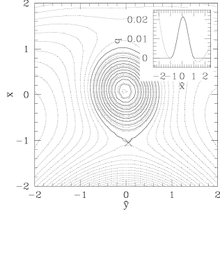
Figure 6: Same as Fig. 5, except for a separation of $\bar{x}_{\rm BH}=11.9\bar{M}_{\rm BH}$ (the center of the black hole is located at $\hat{x}=-4.18$ and $\hat{y}=0$). The Lagrange point $L_{1}$ is now located on the star’s surface, indicating the onset of tidal disruption.

$\hat{x}_{\rm BH}$	$x_{\rm BH}/M_{\rm BH}$	$\bar{r}_{e}$	$q_{\rm max}$	$\Omega M_{\rm BH}$
- 8.0	17.8	1.11	0.0235	0.0133
- 5.0	12.6	1.26	0.0223	0.0223
- 4.74	12.3	1.30	0.0221	0.0230
- 4.49	12.1	1.35	0.0220	0.0236
- 4.34	12.0	1.38	0.0219	0.0239
- 4.18	11.9	1.42	0.0218	0.0241

Table 1: Numerical values for a constant rest-mass sequence with $\bar{M}_{\rm BH}=0.5$ and $\bar{M}_{\rm NS}=0.05$ close to the onset of tidal disruption at a separation of $x_{\rm BH}=11.9M_{\rm BH}$ (see Fig. 6).

In corotating binaries, tidal disruption occurs when the neutron star overflows its Roche lobe. In Newtonian physics, the Roche lobe is defined as the innermost equipotential surface of the effective potential (17) that encompasses both binary companions. In a contour plot in the equatorial plane the Roche lobe forms a “figure eight”, in which each teardrop-shaped region contains one companion. The equipotenial surface pinches off at the saddle-point of the potential, which is called the inner Lagrange point $L_{1}$. When the neutron star overflows its Roche lobe, matter flows across this inner Lagrange point and accrets onto the black hole.

By virtue of the integrated Euler equation (16) the density parameter $q$ is proportional, up to a constant, to the effective potential $\Phi_{\rm eff}$. The Roche lobe can therefore be constructed equivalently from contours of the right hand side of the integrated Euler equation (16). This immediately suggests the construction of a relativistic Roche lobe from the right hand side of the integrated relativistic Euler equation (48). For a relativistic equilibrium configuration, the Roche lobe and Lagrange points can therefore be identified in complete analogy to the Newtonian case.

In Figs. (5) and (6) we show contours for two configurations with $\bar{M}_{\rm NS}=\bar{M}_{\rm BH}/10=0.05$ in the equatorial plane. Table 1 also provides numerical values for this sequence. Fig. (5) shows the binary at a separation of $\bar{x}_{\rm BH}=12.6\bar{M}_{\rm BH}$ (the second line in Table 1). For this calculation and all others in this Section we used a grid of $(48\times 48\times 24)$ gridpoints and imposed outer boundaries at $\hat{X}_{\rm out}$ = 3. Density contours are marked by solid lines, while contours of the right hand side of (48), i.e. contours of the relativistic effective potential, are marked by the dotted lines. The inner Lagrange point $L_{1}$ is marked by the cross. The contour passing through this point is the Roche lobe. The outermost solid contour, which marks the surface of the star, is still inside the Roche lobe, so tidal disruption has not yet set in.

In Fig. (6) we show the same binary, but at a slightly smaller separation of $\bar{x}_{\rm BH}=11.9\bar{M}_{\rm BH}$ (the last line in Table 1). Now the Lagrange point $L_{1}$, again marked by a cross, is located on the surface of the star, indicating that the star now fills out its Roche lobe, and that tidal disruption sets in. This illustrates how the onset of tidal disruption can be identified by the Lagrange point $L_{1}$ reaching the surface of the star, and simultaneously the star filling out its Roche lobe.

Figure 7: The tidal separation $s_{\rm tid}/R_{\rm NS}$ as a function of mass ratio $M_{\rm NS}/M_{\rm BH}$. The crosses mark our numerical results for $\bar{M}_{\rm NS}=0.01$, the dot marks a result obtained by Uryū & Eriguchi ue99 , and the solid line denotes the expected qualitative scaling relation (3), $(M_{\rm NS}/M_{\rm BH})^{-1/3}$. The dashed line, $2.35(M_{\rm NS}/M_{\rm BH})^{-1/3}$, provides an approximate fit to our numerical data.

$M_{\rm NS}/M_{\rm BH}$	$x_{\rm BH}/M_{\rm BH}$	$s_{\rm tid}/R_{\rm NS}$	$\Omega M_{\rm BH}$
0.01	13.3	11.0	0.0203
0.02	20.9	8.67	0.0102
0.05	38.5	6.43	0.00405
0.1	61.7	5.18	0.00199
0.1	—	5.17	0.00208

Table 2: Numerical values for the onset of tidal disruption of an $\bar{M}_{\rm NS}=0.01$ neutron star (whose isotropic radius in isolation is $\bar{R}_{\rm NS}=1.23$). The bottom line are the results from the Newtonian models of Uryū & Eriguchi ue99 (see their Table 2).

It is now of interest to see whether we recover the scaling (3). To better compare with Uryū & Eriguchi ue99 , who have located the tidal separation in Newtonian BHNS binaries, we compute their measure of separation

$$s_{\rm tid}=x_{\rm BH}+\frac{1}{M_{\rm NS}}\int x\rho d^{3}x$$ (71)

(denoted $d_{G}$ in ue99 .) In Table 2 and Fig. 7 we show results for $\bar{M}_{\rm NS}=0.01$, for which $R_{\rm NS}/M_{\rm NS}=123$. For these configurations relativistic effects are sufficiently weak to make a comparison with Newtonian results meaningful. According to the scaling relation (4), tidal disruption will occur over a reasonable range of mass ratios $M_{\rm NS}/M_{\rm BH}\ll 1$. Crosses in Fig. (7) denote results from our code, and the dot marks the only result from ue99 for $n=1$ and $M_{\rm NS}/M_{\rm BH}\leq 0.1$ (see also the bottom line in Table 2). Our result agrees with that of ue99 to within a few percent (and even better for the tidal separation $s_{\rm tid}$), which is well within the error that one expects for a mass ratio of $M_{\rm NS}/M_{\rm BH}=0.1$ within our approximation $M_{\rm NS}/M_{\rm BH}\ll 1$. For this configuration both $M_{\rm NS}/R_{\rm NS}\approx 0.01$ and $M_{\rm BH}/s_{\rm tid}\approx 0.01$ so that relativistic effects could also introduce a deviation of a few percent.

The scaling of the tidal separation with the mass ratio is very close to that predicted by (3); in fact, the crude estimate for the tidal separation differs by only about a factor of 2.35 from our numerical results.

VI Summary

We have developed a new relativistic formalism for the construction of BHNS binaries in quasiequilibrium. We solve the constraint equations of general relativity, decomposed in the thin-sandwich formalism, together with the integrated Euler equation for the neutron star matter. The background geometry describes a Schwarzschild black hole, which accounts for the neutron star’s binary companion. Our approach yields self-consistent solutions describing a neutron star and its self-gravity in the presence of a black hole companion.

In this paper we assume that the black hole mass is much larger than that of the neutron star, which simplifies the problem in a number of ways. In this case, the axis of rotation, which in general is located at the binary center of mass, passes through the center of the black hole. Also in this limit, we can assume that the neutron star only affects the spacetime in a neighborhood around the star, so that the numerical grid can be restricted to such a neighborhood and does not need to cover the black hole. This eliminates the need for black hole excision. Furthermore, it is appropriate to assume that the black hole’s irreducible mass, which is essentially constant during a quasiequilibrium inspiral, is equal to the background mass, which eliminates the need for an iteration.

Adopting this approximation, we have tested our code for isolated neutron stars and for constant rest mass sequences, finding excellent agreement with Kepler’s third law for the orbital frequency. We have also developed a fully relativistic framework for the identification of the Roche lobe and Lagrange points, which can be used to locate the binary separation at which tidal break-up sets in. For weakly relativistic $n=1$ polytropes, for which the tidal separation is outside of the innermost stable circular orbit even for large mass ratios, we find that tidal disruption occurs at about twice the separation suggested by the crude scaling relation $s_{\rm tid}/R_{\rm NS}\sim(M_{\rm BH}/M_{\rm NS})^{1/3}$.

Astrophysically more interesting scenarios require $M_{\rm BH}\sim M_{\rm NS}$, for which the above assumption of extreme mass ratios has to be relaxed. We plan to provide solutions to black hole – neutron star binaries with companions of comparable mass in the near future.

Appendix A Numerical Strategy

In this Appendix we provide details on the numerical strategy and implementation for the solution of the field equations (51) – (53), together with the integrated Euler equation (55).

A.1 Numerical Grid

The only symmetry assumption that can be made to simplify the problem is equatorial symmetry across the $z=0$ plane. In the Newtonian case, or in the case of maximal slicing $K=0$, the solutions are also symmetric across the $y=0$ plane. But the presence of a non-zero $K$ as in the case considered here there is no such symmetry condition across the $y=0$ plane (see also Appendix E in ycsb04 ). The numerical grid can therefore be chosen to cover a region $\hat{x}_{\rm min}\leq\hat{x}\leq\hat{x}_{\rm max}$, $\hat{y}_{\rm min}\leq\hat{y}\leq\hat{y}_{\rm max}$ and $0\leq\hat{z}\leq\hat{z}_{\rm max}$. For the results in this paper we chose the limits to be the same in all dimensions, $-\hat{x}_{\rm min}=\hat{x}_{\rm max}=-\hat{y}_{\rm min}=\hat{y}_{\rm max}=\hat{z}_{\rm max}=\hat{X}_{\rm out}$. In this paper we also assume that $M_{\rm BH}\gg M_{\rm NS}$ and restrict the numerical grid to a neighborhood of the neutron star, which requires $\hat{X}_{\rm out}<\hat{x}_{\rm BH}$ (the origin of the coordinate system is at the center of the neutron star, compare Fig. 1).

A.2 Elliptic Solver

A variety of different approaches can be chosen to solve the elliptic equations (51) – (53), together with the algebraic equation (55). We adopt finite difference methods, and solve the resulting finite difference equations on uniform grids in a parallel environment using DAGH software DAGH . Having adopted a Kerr-Schild background, the operators in equations (51) – (53) are not flat, which poses an additional challenge. One possible method of solving such a problem is to replace the “covariant Laplace” operator with a flat Laplace operator and solve the equation iteratively. In this paper we instead use PETSc software PETSC to solve linear elliptic equations of the form

$$\hat{D}^{2}f+u_{f}f=r_{f}$$ (72)

directly. Here $\hat{D}^{2}$ is a covariant Laplace operator

$$\hat{D}^{2}f=\hat{\gamma}^{ij}f_{,ij}-\hat{\Gamma}^{i}f_{,i}$$ (73)

and $u_{f}$ and $r_{f}$ are functions. In the following we assume that the metric $\hat{\gamma}^{ij}$ and the connection coefficients $\hat{\Gamma}^{i}$ are given by the background quantities (64) and (66). Equations (51) – (53) can then be solved by casting them into the form (72).

A.3 Hamiltonian Constraint

We write the conformal factor as a sum of contributions from the black hole and the neutron star

$$\psi=\psi_{\rm BH}+\psi_{\rm NS}.$$ (74)

In the absence of the neutron star the background metric $\hat{\gamma}_{ij}$ is already a solution to the constraints, so

$$\psi_{\rm BH}=1$$ (75)

identically. The split (74) is convenient since $\psi_{\rm NS}$ now satisfies a Robin fall-off conditions at large separation from the neutron star.

Since the Hamiltonian constraint (51) contains non-linear terms, the equation has to be linearized before it can be solved with the linear operator (72). A solution to the non-linear problem is then constructed iteratively. We therefore write the solution $\psi_{\rm NS}$ as a sum of the previous result $\Psi_{\rm NS}$ and a correction $\delta\psi_{\rm NS}$,

$$\psi_{\rm NS}=\Psi_{\rm NS}+\delta\psi_{\rm NS}.$$ (76)

Inserting this into (74) and (51) then yields, to first order in $\delta\psi_{\rm NS}$,

$$\hat{D}^{2}\delta\psi_{\rm NS}-$$ (77)

$$\delta\psi_{\rm NS}\left(\frac{1}{8}\hat{R}+\frac{5}{12}\Psi^{4}\hat{K}^{2}+\frac{7}{8}\Psi^{-8}\hat{A}^{2}-10\pi\Psi^{4}\bar{r}_{e}^{2}\bar{\rho}\right)$$

$$=-\hat{D}^{2}\Psi+\frac{1}{8}\Psi\hat{R}+\frac{1}{12}\Psi^{5}\hat{K}^{2}-\frac{1}{8}\Psi^{-7}\hat{A}^{2}-2\pi\Psi^{5}\bar{r}_{e}^{2}\bar{\rho}$$

where we have used the abbreviations

$$\Psi=1+\Psi_{\rm NS}$$ (78)

and

$$\hat{A}^{2}=\hat{A}_{ij}\hat{A}^{ij}.$$ (79)

Defining the residual of equation (51) as

$$\mbox{Res}_{\psi}\equiv\hat{D}^{2}\psi-\frac{1}{8}\psi\hat{R}-\frac{1}{12}\psi^{5}\hat{K}^{2}+\frac{1}{8}\psi^{-7}\hat{A}^{2}+2\pi\psi^{5}\bar{r}_{e}^{2}\bar{\rho}$$ (80)

we can rewrite equation (77) in the form (72) with

$$u_{\delta\psi_{\rm NS}}=-\left(\frac{1}{8}\hat{R}+\frac{5}{12}\Psi^{4}\hat{K}^{2}+\frac{7}{8}\Psi^{-8}\hat{A}^{2}-10\pi\Psi^{4}\bar{r}_{e}^{2}\bar{\rho}\right)$$ (81)

and

$$r_{\delta\psi_{\rm NS}}=-\mbox{Res}_{\Psi}$$ (82)

As discussed in Section A.9 we usually drop the linearized matter term $10\pi\Psi^{4}\bar{r}_{e}^{2}\bar{\rho}$ in equation (81) above. This does not affect the final solution, and while removing this term slowed down the solution of the individual equation, it did improve the convergence of the overall iteration scheme.

In the above equations the background scalar curvature $\hat{R}$ is given by

$$\hat{R}=8\frac{\alpha^{4}_{\rm BH}H^{2}}{\hat{r}_{\rm BH}^{2}},$$ (83)

and $\hat{A}_{ij}$ is computed from equation (54) (see Section A.6 below).

A.4 The lapse equation

It is convenient to introduce a new variable

$$N=\alpha\psi,$$ (84)

in terms of which equation (53) can be rewritten as

$$\hat{D}^{2}N - \frac{7}{8}N\psi^{-8}\hat{A}^{2}-\frac{5}{12}N\psi^{4}\hat{K}^{2}-\frac{1}{8}N\hat{R}-\psi^{5}\beta^{i}\hat{D}_{i}\hat{K}$$ (85)

$$= 2\pi N\psi^{4}\bar{r}_{e}^{2}(\bar{\rho}+2\bar{S}).$$

Similar to the split (74) we write $N$ as contributions from the black hole and the neutron star

$$N=N_{\rm BH}+N_{\rm NS}.$$ (86)

In the absence of the neutron star $N_{\rm BH}$ reduces to $\alpha_{\rm BH}$, so we may identify

$$N_{\rm BH}=\alpha_{\rm BH}$$ (87)

The split (86) can now be inserted into (85), which results in an equation of the form (72) with

$$u_{N_{\rm NS}}=-\frac{7}{8}\psi^{-8}\hat{A}^{2}-\frac{5}{12}\psi^{4}\hat{K}^{2}-\frac{1}{8}\hat{R}-2\pi\psi^{4}\bar{r}_{e}^{2}(\bar{\rho}+2\bar{S})$$ (88)

and

$$r_{N_{\rm NS}} = -\hat{D}^{2}\alpha_{\rm BH}+\frac{7}{8}\alpha_{\rm BH}\psi^{-8}\hat{A}^{2}+\frac{5}{12}\alpha_{\rm BH}\psi^{4}\hat{K}^{2}$$

$$+\frac{1}{8}\alpha_{\rm BH}\hat{R}+\psi^{5}\beta^{i}\hat{D}_{i}K+2\pi\alpha_{\rm BH}\psi^{4}\bar{r}_{e}^{2}(\bar{\rho}+2\bar{S})$$

where

$$\hat{D}^{2}\alpha_{\rm BH}=\frac{4\alpha_{\rm BH}^{7}H^{2}}{\hat{r}_{\rm BH}^{2}}.$$ (90)

A.5 The Momentum Constraint

We first split the shift vector into contributions from the black hole, the neutron star, and a rotational term

$$\beta^{i}=\beta^{i}_{\rm BH}+\beta^{i}_{\rm NS}+\xi^{i},$$ (91)

where

$$\xi^{i}=\epsilon^{ijk}\hat{\Omega}_{j}\hat{x}_{k}=\hat{\Omega}(-\hat{y},\hat{x}-\hat{x}_{\rm rot},0).$$ (92)

In equation (52), the analytic contributions can be moved to the right hand side, leaving an equation for the neutron star contribution

$$\hat{\Delta}_{L}\beta^{i}_{\rm NS} = 2\hat{A}^{ij}\hat{D}_{j}(\alpha\psi^{-6})+\frac{4}{3}\alpha\hat{D}^{i}\hat{K}$$ (93)

$$+16\pi\alpha\psi^{4}\bar{r}_{e}^{2}\bar{\jmath}^{i}-\hat{\Delta}_{L}\beta^{i}_{\rm BH}-\hat{\Delta}_{L}\xi^{i}$$

$$\equiv S^{i}.$$

This equation can be solved with appropriate boundary conditions for $\beta^{i}_{\rm NS}$ alone.

The individual terms in (93) are computed as follows. The first term on the right hand side is written as

$$2\hat{A}^{ij}\hat{D}_{j}(\alpha\psi^{-6})=2\hat{A}^{ij}\hat{D}_{j}(N\psi^{-7})$$ (94)

$$=2\hat{A}^{ij}\psi^{-7}(\hat{D}_{j}\alpha_{\rm BH}+\hat{D}_{j}N_{\rm NS}-7N\psi^{-1}\hat{D}_{j}\psi).$$

Here the first term can be computed analytically from the Kerr-Schild background

$$\hat{D}_{j}\alpha_{\rm BH}=\frac{\alpha_{\rm BH}^{3}H}{\hat{r}_{\rm BH}}l_{j}.$$ (95)

The gradient of $K$ in (93) is written as

$$\frac{4}{3}\alpha\hat{D}^{i}\hat{K} = \frac{4N}{3\psi}\hat{D}^{i}\hat{K}$$

$$= -\frac{\alpha_{\rm BH}+N_{\rm NS}}{\psi}\,\frac{8\alpha_{\rm BH}^{7}H}{3\hat{r}_{\rm BH}^{2}}(2+10H+9H^{2})l^{i}.$$

The vector Laplacian of $\beta^{i}_{\rm BH}$ is given by

$$\hat{\Delta}_{L}\beta^{i}_{\rm BH}=-\frac{8\alpha_{\rm BH}^{8}H}{3\hat{r}_{\rm BH}^{2}}(2+12H+12H^{2})l^{i}.$$ (97)

We note that in the absence of a neutron star, $N_{\rm NS}=\psi_{\rm NS}=\hat{\Omega}=\bar{\jmath}^{i}=0$, equation (93) is satisfied analytically with $\beta^{i}_{\rm NS}=0$.

The next goal is to bring the operator

$$\hat{\Delta}_{L}\beta^{i}_{\rm NS}=\hat{D}^{2}\beta^{i}_{\rm NS}+\frac{1}{3}\hat{D}^{i}\hat{D}_{j}\beta_{\rm NS}^{j}+\hat{R}^{i}_{~{}j}\beta_{\rm NS}^{j}$$ (98)

into the form (72). The mixed second derivatives can be eliminated by writing $\beta^{i}_{\rm NS}$ as the sum of a vector and the gradient of a scalar

$$\beta^{i}_{\rm NS}=W^{i}+\frac{1}{4}\hat{D}^{i}U.$$ (99)

With this choice, equation (93) can be written as

$$\hat{D}^{2}U=-\hat{D}_{i}W^{i}$$ (100)

and

$$\hat{D}^{2}W^{i}=S^{i}-\hat{R}^{i}_{~{}j}\left(W^{j}+\frac{1}{2}\hat{D}^{j}U\right).$$ (101)

Since $U$ is a scalar, equation (100) is already in the form (72), and can be solved immediately with

$$u_{U} = 0$$ (102)

$$r_{U} = -\hat{D}_{i}W^{i}.$$ (103)

Equation (101) is more complicated. Writing out the covariant Laplace operator acting on a vector, we have

$$\hat{D}^{2}W^{l} = \hat{\gamma}^{ij}W^{l}_{~{},ij}-W^{l}_{~{},k}\hat{\Gamma}^{k}+2\hat{\gamma}^{ij}W^{m}_{~{},i}\hat{\Gamma}^{l}_{mj}$$

$$+W^{m}(\hat{\gamma}^{ij}\hat{\Gamma}^{l}_{mj,i}-\hat{\Gamma}^{l}_{mk}\hat{\Gamma}^{k}+\hat{\gamma}^{ij}\hat{\Gamma}^{k}_{mj}\hat{\Gamma}^{l}_{ki}).$$

It is convenient to define

$$\hat{\Delta}^{l}_{~{}m}\equiv\hat{\gamma}^{ij}\hat{\Gamma}^{l}_{mj,i}-\hat{\Gamma}^{l}_{mk}\hat{\Gamma}^{k}+\hat{\gamma}^{ij}\hat{\Gamma}^{k}_{mj}\hat{\Gamma}^{l}_{ki}$$ (105)

$$=\frac{2\alpha_{\rm BH}^{6}H}{\hat{r}_{\rm BH}^{2}}\left((1+2H)^{2}\eta^{l}_{~{}m}-(3+13H+12H^{2})l^{l}l_{m}\right)$$

so that equation (A.5) becomes

$$\hat{D}^{2}W^{l}=\hat{\gamma}^{ij}W^{l}_{~{},ij}-W^{l}_{~{},k}\hat{\Gamma}^{k}+2\hat{\gamma}^{ij}W^{m}_{~{},i}\hat{\Gamma}^{l}_{mj}+W^{m}\hat{\Delta}^{l}_{~{}m}.$$ (106)

To obtain the equation for $W^{l}$, the third term and the pieces of the fourth term not containing $W^{l}$ can now be moved to the right hand side of equation (101). The term $R^{i}_{~{}i}W^{i}$ (no summation) on the right hand side of (101) can also be absorbed in a $u_{W^{i}}$ on the left hand side, which leaves us with an equation for $W^{i}$ in the form (72) with

$$u_{W^{i}} = \hat{R}^{i}_{~{}i}+\Delta^{i}_{~{}i}~{}~{}~{}~{}~{}\mbox{no summation}$$ (107)

$$r_{W^{i}} = S^{i}-\hat{R}^{i}_{~{}j}W^{j}-\frac{1}{2}\hat{R}^{i}_{~{}l}\hat{D}^{l}U-2W^{m}_{~{},l}\hat{\Gamma}^{il}_{m}$$ (108)

$$-W^{j}\Delta^{i}_{~{}j}~{}~{}~{}~{}~{}(j\neq i).$$

Here we have defined

$$\hat{\Gamma}^{li}_{m} \equiv \hat{\gamma}^{ij}\hat{\Gamma}^{l}_{mj}$$

$$= \frac{\alpha_{\rm BH}^{4}H}{\hat{r}_{\rm BH}}\left(2(1+2H)l^{l}\eta^{i}_{~{}m}-(3+4H)l^{l}l^{i}l_{m}\right).$$

We also note that

$$\hat{R}^{i}_{~{}j}=$$ (110)

$$\frac{\alpha^{6}_{\rm BH}H}{\hat{r}^{2}_{\rm BH}}\left((1+6H+8H^{2})\eta^{i}_{~{}j}-(3+10H+8H^{2})l^{i}l_{j}\right).$$

In $S^{i}$, $\hat{\Delta}_{L}\xi^{i}$ can be computed from (36) and (A.5). The partial derivatives can be computed trivially from (92); in particular we have $\xi^{l}_{,ij}=0$. Because of the symmetries we also have $\xi^{m}_{~{},i}\hat{\Gamma}^{li}_{m}=0$, which simplifies the calculation. For extreme mass ratios, when $x_{\rm rot}=x_{\rm BH}$, $\hat{\Delta}_{L}\xi^{i}=0$ identically. Equation (101) can now be solved iteratively for the components $W^{i}$.

A.6 The Extrinsic Curvature

With a new solution for the shift $\beta^{i}$, the extrinsic curvature $\hat{A}^{ij}$ can be computed from equation (54). In this expression, the shift decomposition (91) has to be inserted. The background contribution of $\beta^{i}_{\rm BH}$ can be computed analytically

$$(\hat{L}\beta_{\rm BH})^{ij}=$$ (111)

$$\frac{4\alpha^{6}_{\rm BH}H}{3\hat{r}_{\rm BH}}\left((2+7H+6H^{2})\eta^{ij}-(6+13H+6H^{2})l^{i}l^{j}\right).$$

The contributions of the rotational term $\xi^{i}$ are most easily added by calculating the partial derivatives directly from (92), and computing the connection terms together with those for the neutron star terms $\beta^{i}_{\rm NS}$.

A.7 The integrated Euler equation

As in the Newtonian case we first evaluate the integrated Euler equation (48) at the three points $\hat{x}_{A}$, $\hat{x}_{B}$ and $\hat{x}_{C}$ to find the three eigenvalues $C$, $\hat{\Omega}$ and $\bar{r}_{e}$. All quantities in the integrated Euler equation have to be expressed in terms of our decompositions (74), (86) and (91). Of the three constants, only $C$ appears directly in (48). The angular velocity $\hat{\Omega}$ has also been introduced explicitly through the rotational shift term $\xi^{i}$ in (91). The scaling parameter $\bar{r}_{e}$ again only appears through the implicit scaling of the gravitational potentials. In the Newtonian case, the Poisson equation (19) immediately implied a scaling for $\phi_{\rm NS}$. The corresponding relativistic field equations, namely the Hamiltonian constraint (51) and the lapse equation (53), do not provide such a simple scaling because the non-linear terms. However, we can use the Newtonian limit to guess an appropriate scaling (compare bcsst .)

In the Newtonian limit, the lapse becomes

$$\alpha\sim e^{\phi}\sim 1+\phi=1+\phi_{\rm NS}+\phi_{\rm BH}.$$ (112)

Since the background describes a black hole, the conformal factor only includes a neutron star contributions, so that in the Newtonian limit

$$\psi\sim e^{-\phi_{\rm NS}/2}\sim 1-\frac{1}{2}\phi_{\rm NS}.$$ (113)

Comparing with (74) we note that in the Newtonian limit we have

$$\psi_{\rm NS}\sim-\frac{1}{2}\phi_{\rm NS}$$ (114)

and from (86)

$$N_{\rm NS}=\alpha\psi-\alpha_{\rm BH}\sim\frac{1}{2}\phi_{\rm NS}$$ (115)

In analogy with the Newtonian problem, this suggests the definition

$$\hat{\psi}_{\rm NS}=\psi_{\rm NS}/\bar{r}_{e}^{2}~{}~{}~{}~{}~{}~{}~{}~{}~{}\hat{N}_{\rm NS}=N_{\rm NS}/\bar{r}_{e}^{2}$$ (116)

In the integrated Euler equation, $\psi_{\rm NS}$ and $N_{\rm NS}$ can then be replaced with $\bar{r}_{e}^{2}\hat{\psi}_{\rm NS}$ and $\bar{r}_{e}^{2}\hat{N}_{\rm NS}$, which explicitely introduces the scaling parameter $\bar{r}_{e}$ into the equation.

Once the three eigenvalues $C$, $\hat{\Omega}$ and $\bar{r}_{e}$ have been found, $\psi_{\rm NS}$ and $N_{\rm NS}$ have to be rescaled to reflect the new value of $\bar{r}_{e}$. The integrated Euler equation can then be solved everywhere for the new density distribution $q$.

A.8 Boundary Conditions

In general, the construction of BHNS binaries requires three different kinds of boundary conditions: exterior boundary conditions at large separation from the binary, inner boundary conditions on the black hole’s excision surface, and, having adopted equatorial symmetry (see Section A.1), a symmetry boundary condition on the $z=0$ plane. The symmetry conditions on the $z=0$ are straight-forward to implement (see Table 3). As explained in Section IV, the assumption of extreme mass ratios $M_{\rm BH}\gg M_{\rm NS}$ allows us to restrict the numerical grid to a region around the neutron star. This eliminates the need for interior excision boundary conditions, but it also requires imposing boundary conditions in the potentially strong-field regime close to the black hole.

Given that we expect the neutron star to affect the spacetime only in a small neighborhood, it is reasonable to assume $1/r$ Robin fall-off conditions for the conformal factor $\psi_{\rm NS}$ and lapse $N_{\rm NS}$.

	$z=0$	OB
$\psi_{\rm NS}$	SYM	$\sim\displaystyle\frac{1}{r}$
$N_{\rm NS}$	SYM	$\sim\displaystyle\frac{1}{r}$
$U$	SYM	$\sim\displaystyle\frac{y}{r}$
$W^{x}$	SYM	$\sim\displaystyle\frac{1}{r}$
$W^{y}$	SYM	$\sim\displaystyle\frac{1}{r}$
$W^{z}$	ANTI	$\sim\displaystyle\frac{z}{r^{3}}$

Table 3: Boundary conditions for the outer boundaries (OB) and on the $z=0$ symmetry plane (where SYM denotes symmetric and ANTI antisymmetric boundary conditions). Note the $r$ is the separation from the origin of the coordinate system at the center of the neutron star.

$\hat{X}_{\rm out}$	Grid size	$x_{\rm BH}/M_{\rm BH}$	$r_{e}$	$q_{\rm max}$	$\Omega M_{\rm BH}$
2	$(32\times 32\times 16)$	17.82	1.113	0.02349	0.01330
3	$(48\times 48\times 24)$	17.81	1.113	0.02349	0.01332
4	$(64\times 64\times 32)$	17.81	1.113	0.02349	0.01333
6	$(96\times 96\times 48)$	17.81	1.113	0.02349	0.01336

Table 4: Numerical results for different locations of the outer boundary at constant grid resolution. We show values for a $\bar{M}_{\rm BH}=0.5$, $\bar{M}_{\rm NS}=0.05$ binary at a separation of $\hat{x}_{\rm BH}=-8$ (see also the top line in Table 1).

More subtle are the boundary conditions on the shift quantities $W^{i}$ and $U$. In bcsst a similar decomposition was used for the construction of binary neutron stars, and boundary conditions for these fields were identified from the asymptotic behavior of a multipole solution to a general, but flat vector Laplacian b82 . The construction also assumed that the net momentum contained in the numerical grid vanishes (so that the non-vanishing angular momentum gives rise to the asymptotic fall-off.) Here, however, we solve a vector Laplacian that is not flat, we adopt boundary conditions which are not in an asymptotic region, and the grid containing only the neutron star contains a non-vanishing linear momentum. It is not clear a priori how appropriate boundary conditions on $W^{i}$ and $U$ should be constructed in this case. We have experimented with several different conditions, and did notice some effect on the convergence properties of the iteration scheme. We found reasonable results with the conditions tabulated in Table 3, which are motivated by the construction in b82 but do not assume a vanishing linear momentum. In Table 4 we tabulate numerical values obtained for different locations of the outer boundaries, which demonstrates that our results depend only very weakly on where the outer boundaries are imposed (as long as they are imposed sufficiently far away away from the neutron star and not too close to the black hole singularity). Once the assumption of extreme mass ratios is relaxed and the computational grid encompasses both the neutron star and the black hole, the boundary conditions of bcsst can again be applied.

A.9 Iteration Scheme

The iteration scheme used for the construction of relativistic BHNS binaries is very similar to that for Newtonian binaries described in Section II.5. However, instead of having to solve only one Poisson equation, we now have to solve several Poisson-like equations together with the integrated Euler equation. These different equations can be solved in various different sequences. We found best convergence when solving the integrated Euler equation after each elliptic equation.

We also found that the convergence improved by using underrelaxation, i.e. by using a linear combination

$$f^{n+1}=\chi\tilde{f}^{n+1}+(1-\chi)f^{n},$$ (117)

where $f^{n}$ is any one of the functions $N_{\rm NS}$, $\psi_{\rm NS}$, $W^{i}$ and $U$ after $n$ iteration steps, and $\tilde{f}^{n+1}$ the function after having solved the corresponding elliptic equation. The parameter $\chi$ is the relaxation parameter, and values of $\chi<1$ define underrelaxation. We have found best results for $\chi$ between 0.6 and 0.8.

While the Hamiltonian constraint alone converged faster when solved as described in Section A.3, we also found improved convergence of the overall iteration when we did not include the linearized matter term in equation (81). The effect of not including this term is similar to that of using underrelaxation, and reduced the coupling between the matter and conformal factor, which otherwise led to unstable behavior in some situations.

References

- (1) H.-Th. Janka, T. Eberl, M. Ruffert & C. L. Fryer, Astrophys. J. Lett. 527, L42 (1999).
- (2) M. Vallisneri, Phys. Rev. Lett. 84, 3519 (2000)
- (3) G. B. Cook, Phys. Rev. D 50, 5025 (1994).
- (4) T. W. Baumgarte, Phys. Rev. D 62, 024018 (2000).
- (5) E. Gourgoulhon, P. Grandclément & S. Bonazzola, Phys. Rev. D 65, 044020 (2002); P. Grandclément, E. Gourgoulhon & S. Bonazzola, Phys. Rev. D 65, 044021 (2002).
- (6) J. R. Wilson & G. J. Mathews, Phys. Rev. Lett. 75, 4161 (1995); J. R. Wilson, G. J. Mathews & P. Marronetti, Phys. Rev. D 54, 1317 (1996).
- (7) T. W. Baumgarte, G. B. Cook, M. A. Scheel, S. L. Shapiro & S. A. Teukolsky, Phys. Rev. Lett 79, 1182 (1997); Phys. Rev. D 57, 7299 (1998).
- (8) K. Uryū, M. Shibata & Y. Eriguchi, Phys. Rev. D 62, 104015 (2000).
- (9) E. Gourgoulhon, P. Grandclément, K. Taniguchi, J.-A. Marck & S. Bonazzola, Phys. Rev. D 63, 064029.
- (10) K. Taniguchi & E. Gourgoulhon, Phys. Rev. D 66 104019 (2002).
- (11) G. B. Cook, Living Rev. Rel. 5, 1 (2000).
- (12) T. W. Baumgarte & S. L. Shapiro, Phys. Rept. 376, 41 (2003).
- (13) M. Miller, gr-qc/0106017 (2001).
- (14) D. Lai, F. A. Rasio & S. L. Shapiro, Astrophys. J. Suppl. 88, 205 (1993).
- (15) K. Taniguchi & T. Nakamura, Prog. Theor. Phys. 96, 693 (1996).
- (16) S. Chandrasekhar, Ellipsoidal Figures of Equilibrium, Yale Univ. Press, New Haven (1969).
- (17) L. G. Fishbone, Astrophys. J. 185, 43 (1973).
- (18) M. Shibata, Prog. Theor. Phys., 96, 917 (1996).
- (19) P. Wiggins & D. Lai, Astrophys. J. 532, 530 (2000).
- (20) K. Uryū & Y. Eriguchi, Mon. Not. R. Astro. Soc. 303 329 (1999).
- (21) W. H. Lee, Mon. Not. R. Astro. Soc. 328 583 (2001).
- (22) S. Kobayashi, P. Laguna, E. Sterl Phinney, & P. Mezaros, astro-ph/0404173.
- (23) S. Komossa, J. Halpern, N. Schartel, G. Hasinger, M. Santos-Lleo, & P. Predehl, Astrophys. J. 603, L17 (2004); J.P. Halpern, S. Gezari, & S. Komossa, Astrophys. J. 604, 572 (2004).
- (24) J. W. York, Jr, Phys. Rev. Lett. 82, 1350 (1999).
- (25) L. Bildsten & C. Cutler, Astrophys. J. 400, 175 (1992).
- (26) We point out that bc92 do not consider the extreme mass ratio limit. However, from their equation (8) it is clear that extreme mass ratios lead to an even more severe constraint, making it even more unlikely for neutron stars to be corotational. Physically, tidal effects on the neutron star are less important for much larger companion masses; similarly, the neutron star tidal dissipation timescale increases even more rapidly than the inspiral timescale as the black hole-to-neutron star mass ratio increases.
- (27) R. Arnowitt, S. Deser & C. W. Misner, in Gravitation: An Introduction to Current Research, ed. L. Witten, Wiley, New York (1962) (see also gr-qc/0405109).
- (28) S. Chandrasekhar, The Mathematical Theory of Black Holes, Oxford University Press, New York (1992).
- (29) K. Martel & E. Poisson, Am. J. Phys. 69, 476 (2001).
- (30) R. A. Matzner, M. F. Huq, & D. Shoemaker, Phys. Rev. D 59 024015 (1999).
- (31) P. Marronetti & R. A. Matzner, Phys. Rev. Lett. 85 5500 (2000).
- (32) H. P. Pfeiffer, G. B. Cook & S. A. Teukolsky, Phys. Rev. D 66 024047 (2002).
- (33) M. L. Skoge & T. W. Baumgarte, Phys. Rev. D 66 107501 (2002).
- (34) J. R. Oppenheimer & G. Volkoff, Phys. Rev 55, 374 (1939).
- (35) In the neighborhood of the black hole, deviations of the conformal factor from unity are in the order of . Assuming that the fractional deviation of irreducible mass from the background mass is proportional to the deviation of the conformal factor from unity, , then implies that the absolute deviation is proportional to the binding energy .
- (36) H.-J. Yo, J. N. Cook, S. L. Shapiro & T. W. Baumgarte, submitted (also gr-qc/0406020).
- (37) See http://www.caip.rutgers.edu/ parashar/DAGH/.
- (38) S. Balay, K. Buschelman, W.D. Gropp, D. Kaushik, M. Knepley, L.C. McInnes, B.F. Smith and H. Zhang, PETSc Users Manual ANL-95/11 - Revision 2.1.5. Argonne National Laboratory (2002).
- (39) J. M. Bowen, Gen. Rel. Grav. 14, 1183 (1982).