Jet launching from binary black hole-neutron star mergers: Dependence on black hole spin, binary mass ratio, and magnetic field orientation

Abstract

Black hole-neutron star (BHNS) mergers are one of the most promising targets for multimessenger astronomy. Using general relativistic magnetohydrodynamic simulations of BHNS undergoing merger we previously showed that a magnetically–driven jet can be launched by the disk + spinning black hole remnant if the neutron star is endowed with a dipole magnetic field extending from the interior into the exterior as in a radio pulsar. These self-consistent studies considered a BHNS system with mass ratio $q=3:1$, black hole spin $a/M_{\rm BH}=0.75$ aligned with the total orbital angular momentum, and a neutron star that is irrotational, threaded by an aligned magnetic field, and modeled by an $\Gamma$–law equation of state with $\Gamma=2$. Here, as a crucial step in establishing BHNS systems as viable progenitors of central engines that power short gamma–ray bursts (sGRBs) and thereby solidify their role as multimessenger sources, we survey different BHNS configurations that differ in the spin of the BH companion ($a/M_{\rm BH}=-0.5,\,0,\,0.5,\,0.75$), in the mass ratio ($q=3:1$ and $q=5:1$), and in the orientation of the magnetic field (aligned and tilted by $90^{\circ}$ with respect to the orbital angular momentum). We find that by $\Delta t\sim 3500M-4000M\sim 88(M_{\rm NS}/1.4M_{\odot}){\rm ms}-100(M_{\rm NS}/1.4M_{\odot})\rm ms$ after the peak gravitational wave signal a magnetically–driven jet is launched in the cases where the initial spin of the BH companion is $a/M_{\rm BH}=0.5$ or $0.75$. The lifetime of the jets [$\Delta t\sim 0.5(M_{\rm NS}/1.4M_{\odot}){\rm s}-0.7(M_{\rm NS}/1.4M_{\odot})\rm s$] and their outgoing Poynting luminosities [$L_{jet}\sim 10^{51\pm 1}\rm erg/s$] are consistent with typical sGRBs, as well as with the Blandford–Znajek mechanism for launching jets and their associated Poynting luminosities. By the time we terminate our simulations, we do not observe either an outflow or a large-scale magnetic field collimation in the other configurations we simulate. These results suggest that future multimessenger detections from BHNSs are more likely produced by binaries with highly spinning BH companions and small tilt-angle magnetic fields, though other physical processes do not considered here, such as neutrino annihilation, may help to power jets in general cases.

I Introduction

The era of multimessenger astronomy has accelerated with the detection of GW170817 Abbott et al. (2017a), a gravitational wave (GW) signal from the coalescence of a compact binary, accompanied by electromagnetic (EM) counterpart radiation across the EM spectrum (see e.g. Abbott et al. (2017b, c, d); Chornock et al. (2017); Cowperthwaite et al. (2017); Kasen et al. (2017); Nicholl et al. (2017) and reference therein). From the gravitational radiation signal alone, the inferred masses of the individual binary companions are in the broad range of $0.86-2.26\,M_{\odot}$, though the total mass of the system is constrained to be $2.73-3.29\,M_{\odot}$ with $90\%$ confidence Abbott et al. (2017a). These estimates, along with the EM counterparts, and, in particular, the detection of a short gamma–ray burst (sGRB) – GRB 170817A– $1.7$s–following the inferred merger time by the Fermi Gamma-Ray Burst Monitor von Kienlin et al. (2017) and INTEGRAL Savchenko et al. (2017, 2017), as well as the associated kilonova/macronova, demonstrate the presence of matter Abbott et al. (2017b). These observations strongly suggest a merging binary neutron star system (NSNS) as the source of GW170817, although they cannot rule out the possibility that one of the binary companions is a stellar–mass black hole (BH). Recently, a summary of possible low–mass BH formation channels, and routes by which they may arise in binaries with a NS companion, have been presented in Yang et al. (2018).

Due to the limited sensitivity of the current LIGO/Virgo GW laser interferometers there is still an open question regarding the nature of the GW170817 remnant if one assumes that its progenitor is a NSNS system (see e.g. Shibata et al. (2017); Piro et al. (2018); Ai et al. (2018); Yu et al. (2018); Li et al. (2018); Margalit and Metzger (2017); Ruiz et al. (2018)). Using EM constraints on the remnant imposed by the kilonova observations von Kienlin et al. (2017); Savchenko et al. (2017, 2017); Abbott et al. (2017b) along with the GW data, it was argued in Margalit and Metzger (2017) that the GW170817 NSNS remnant resulted in a hypermassive NS (HMNS) undergoing collapse to a BH in $\sim 10^{-2}$s$-1$s. This hypothesis was supported by our GRMHD simulations reported in Ruiz et al. (2018) where we showed that a long-lived, HMNS seeded with a pulsar-like magnetic field does not power magnetically-driven and sustained outflows (jets) believed to be crucial for generating GRBs as in GW170817. The astrophysical implication of these observations create therefore the urgent need to model GWs and EM counterparts from both NSNS and BHNS systems Hinderer et al. (2018).

GW170718 and GRB 170817A provide the best direct confirmation so far that the merger of compact binaries in which at least one NS is involved can be the engine that powers sGRBs. This identification was originally proposed by Paczynski (1986); Eichler et al. (1989); Narayan et al. (1992) and recently demonstrated by self-consistent simulations in full general relativistic magnetohydrodynamics (GRMHD) of merging BHNSs Paschalidis et al. (2015) and merging NSNSs that undergo delayed collapse Ruiz et al. (2016). The numerical studies in Paschalidis et al. (2015) (hereafter Paper I), whose initial configuration is a BHNS binary with mass ratio $q=3:1$ in a quasicircular orbit, with an NS modeled as an irrotational $\Gamma=2$ polytrope and a BH with dimensionless spin $\tilde{a}\equiv a/M_{\rm BH}=0.75$, showed that a collimated, mildly relativistic outflow –an incipient jet– can be launched from the highly spinning BH remnant surrounded by a magnetized accretion disk. Such a jet requires that a strong poloidal magnetic field component which connects the disk to the BH poles persist after the disruption of the NS Beckwith et al. (2008); Etienne et al. (2012). This key feature was achieved in Paper I by seeding the NS initially with a dipole magnetic field that extends from the stellar interior into the exterior in a pulsar-like, force-free exterior magnetosphere (see e.g. Ruiz et al. (2014)). Following the onset of tidal disruption, it was found that magnetic winding and the magnetorotational instability (MRI) amplify the magnetic field above the BH poles from $\sim 10^{13}(1.4M_{\odot}/M_{\rm NS})$G when the disk first settles to $\sim 10^{15}(1.4M_{\odot}/M_{\rm NS})$G, and this field eventually drives and confines the incipient jet by $\Delta t\sim 100(M_{\rm NS}/1.4M_{\odot})$ms after peak GW emission. The lifetime of the jet and the outgoing Poynting luminosity are $\Delta t\sim 0.5(M_{\rm NS}/1.4M_{\odot})$s and $L_{\rm EM}\sim 10^{51}\rm erg/s$, values which are both consistent with typical sGRBs (see e.g. Bhat et al. (2016); Lien et al. (2016); Svinkin et al. (2016)).

In the NSNS scenario, by contrast, an incipient jet emerges whether or not the initial poloidal magnetic field is confined to the NS interior, as long as the binary forms a HMNS that undergoes delayed collapse to a BH Ruiz et al. (2016). During the formation and spindown of the transient, differentially-rotating HMNS magnetic winding and both the Kelvin-Helmholtz instability and the MRI boost the rms value of the magnetic field to $\gtrsim~{}10^{15.5}$G Kiuchi et al. (2014, 2015). In the prompt collapse scenario, the onset of BH formation following the NSNS merger prevents that amplification Ruiz and Shapiro (2017). The calculations in Ruiz et al. (2016) that model the NS with a simple $\Gamma$–law equation of state (EOS) with $\Gamma=2$, allowing for shock heating, show that the disk + BH remnant launches a jet at about $\sim 44(M_{\rm NS}/1.8M_{\odot})\rm ms$ following the NSNS merger, which lasts $\Delta t\sim 97(M_{\rm NS}/1.8M_{\odot})$ms. The outgoing Poynting luminosity is $L_{\rm EM}\sim 10^{51}\rm erg/s$, consistent with short sGRBs (see e.g. Bhat et al. (2016); Lien et al. (2016); Svinkin et al. (2016)). Recent GRMHD simulations of NSNS mergers reported in Kawamura et al. (2016); Ciolfi et al. (2017), in which the effects of different EOSs, different mass ratios, and different magnetic field orientations with an initial strength of $\sim 10^{12}\rm G$ were studied, did not find evidence of an outflow or a jet after $\Delta t\sim 35\rm ms$ following the NSNS merger, although the formation of an organized magnetic field structure above the BH was observed. A lack of a jet in the high resolution NSNS mergers has been also reported Kiuchi et al. (2014), in which the NS is modeled by an H4 EOS. At the end of those simulations, however, they report persistent fall-back debris in the atmosphere, which increases the ram pressure above the BH poles, preventing the system form approaching a near force-free environment as required for jet launching. A longer time integration may be needed for the atmosphere to disperse and for the jet to emerge. Note that jet launching may not be possible for all EOSs, if the matter fall-back timescale is longer than the disk accretion timescale Paschalidis (2017). The seeded poloidal magnetic field in the numerical studies of Kawamura et al. (2016); Ciolfi et al. (2017); Kiuchi et al. (2014) is restricted to the NS interior.

In this paper, we survey fully relativistic BHNS configurations initially in a quasicircular orbit that undergo merger to address the question: Can all the BHNS configurations that undergo merger in which the NS is seeded with a pulsar-like, force-free magnetic field be progenitors of the engine that launches incipient jets?

In particular, we now consider BHNS configurations with mass ratio $q=3:1$ in which the dimensionless spin of the BH companion is $\tilde{a}=-0.5$ (counter–rotating), $\tilde{a}=0$ (nonspinning), and $\tilde{a}=\,0.5$, all aligned with the orbital angular momentum. In addition, we consider a BHNS configuration with mass ratio $q=5:1$ in which the BH companion has no spin initially. In all cases, the NS is endowed with a dynamically weak poloidal magnetic field that extends from the stellar interior into the NS exterior (i.e. a pulsar-like magnetic field) whose dipole magnetic moment is also aligned with the orbital angular momentum. Finally, to study the effect of different magnetic field topologies on the jet launching, we evolve the same configuration as in Paper I (mass ratio $q=3:1$ and BH spin $\tilde{a}=0.75$) but now seed the NS with a pulsar-like magnetic field whose dipole magnetic moment is tilted $90^{o}$ with respect to the orbital angular momentum. Following Paper I, we model the initial stars as irrotational $\Gamma=2$ polytropes.

In agreement with our earlier calculations, where the star is seeded with a dipole magnetic field confined to the stellar interior Etienne et al. (2008, 2012a), we find that the BHNS mergers listed above lead to a disk + BH remnant with a rest-mass ranging from $\sim 10^{-3}M_{\odot}(k/189.96\rm km^{2})^{1/2}$ to $\sim 10^{-1}M_{\odot}(k/189.96\rm km^{2})^{1/2}$, and dimensionless spin ranging from $\tilde{a}\sim 0.33$ to $\sim 0.85$. Here $k$ is the polytropic gas constant defined as $k=P/\rho_{0}^{\Gamma}$, where $P$ and $\rho_{0}$ are the initial cold pressure and the rest-mass density (see below). The early evolution, tidal disruption and the merger phases are unaltered by the dynamically weak initial magnetic field. In the post-merger phase we find that, as in Paper I, by around $\Delta t\sim 3500M\approx 88(M_{\rm NS}/1.4M_{\odot})\rm ms$ after the GW peak emission a magnetically–driven jet is launched in the case where the initial spin of the BH companion is $\tilde{a}=0.5$. The lifetime of the jet [$\Delta t\sim 0.7(M_{\rm NS}/1.4M_{\odot})\rm s$] and outgoing Poynting luminosity [$L_{jet}\sim 10^{52}\rm erg/s$] are consistent with observations of sGRBs (see e.g. Bhat et al. (2016)), as well as with the Blandford–Znajek (BZ) Blandford and Znajek (1977a) mechanism for launching jets and their associated Poynting luminosities Thorne et al. (1986). In contrast, by the time we terminate our simulations, we do not find any indication of an outflow in the other cases; in the nonspinning case ($\tilde{a}=0$), where a persistent fall-back debris toward the BH is observed until the end of the simulation, the magnetic field above the BH poles is wound into a helical configuration, but the magnetic pressure gradients are still too weak to overcome the fall-back ram pressure, and thus it is expected that a longer simulation is required if a jet were to emerge. However, if the fall-back debris timescale is longer than the disk accretion timescale [$\Delta t\sim 0.36(M_{\rm NS}/1.4M_{\odot})\rm s$], the jet launching in this case may be suppressed. By contrast, in the counter rotating BHNS configuration the star plunges quickly into the BH, leaving an “orphan” BH with a negligibly small accretion disk containing less than $1\%$ of the rest-mass of the NS. Similar behavior is observed in the BHNS configuration with mass ratio $q=5:1$. Finally, in the tilted magnetic field case, we do not find a coherent poloidal magnetic field component remaining after the BHNS merger, hence the key ingredient for jet launching Beckwith et al. (2008) is absent.

These preliminary results suggest that jet launching may strongly depend on a threshold value of (a) the initial black hole spin, which, along with the tidal-break up separation, controls the mass of the accretion disk, and (b) the tilt-angle of the magnetic field, which triggers the presence of a poloidal component of the magnetic field in the post-merger phase. So future multimessenger detections from BHNSs are most likely produced by binaries with a highly–spinning BH companion and small tilt-angle magnetic fields (see also Bhattacharya et al. (2018)).

The remainder of the paper is organized as follows: A short summary of our numerical methods and their implementation is presented in Sec. II.1. A detailed description of our adopted initial data and the grid structure used for solving the GRMHD equations is given in Sec. II.2 and Sec. II.3, respectively. In Sec. II.4 we describe the diagnostics employed to monitor and verify the reliability of our numerical calculations. We present our results in Sec. III, along with a comparison with the results of Paper I, as well as with the ”universal” analytic model presented in Shapiro (2017). Finally, we offer conclusions in Sec. IV. We adopt geometrized units ($G=c=1$) throughout the paper except where stated explicitly. Greek indices denote all four spacetime dimensions, while Latin indices imply spatial parts only.

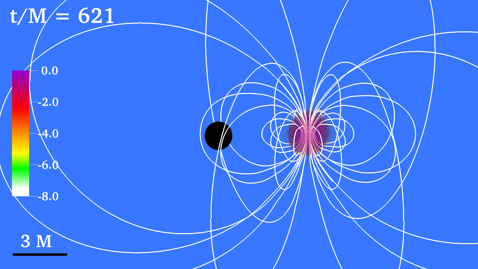
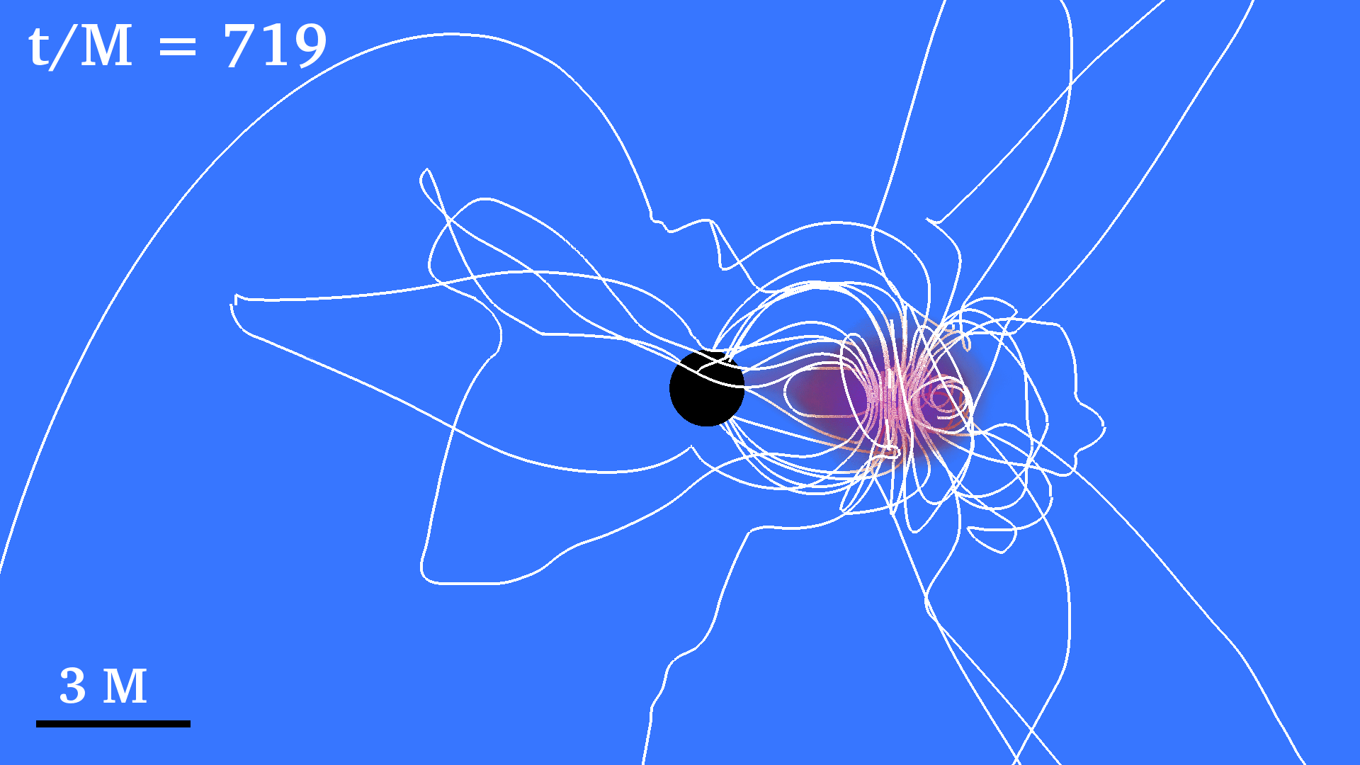
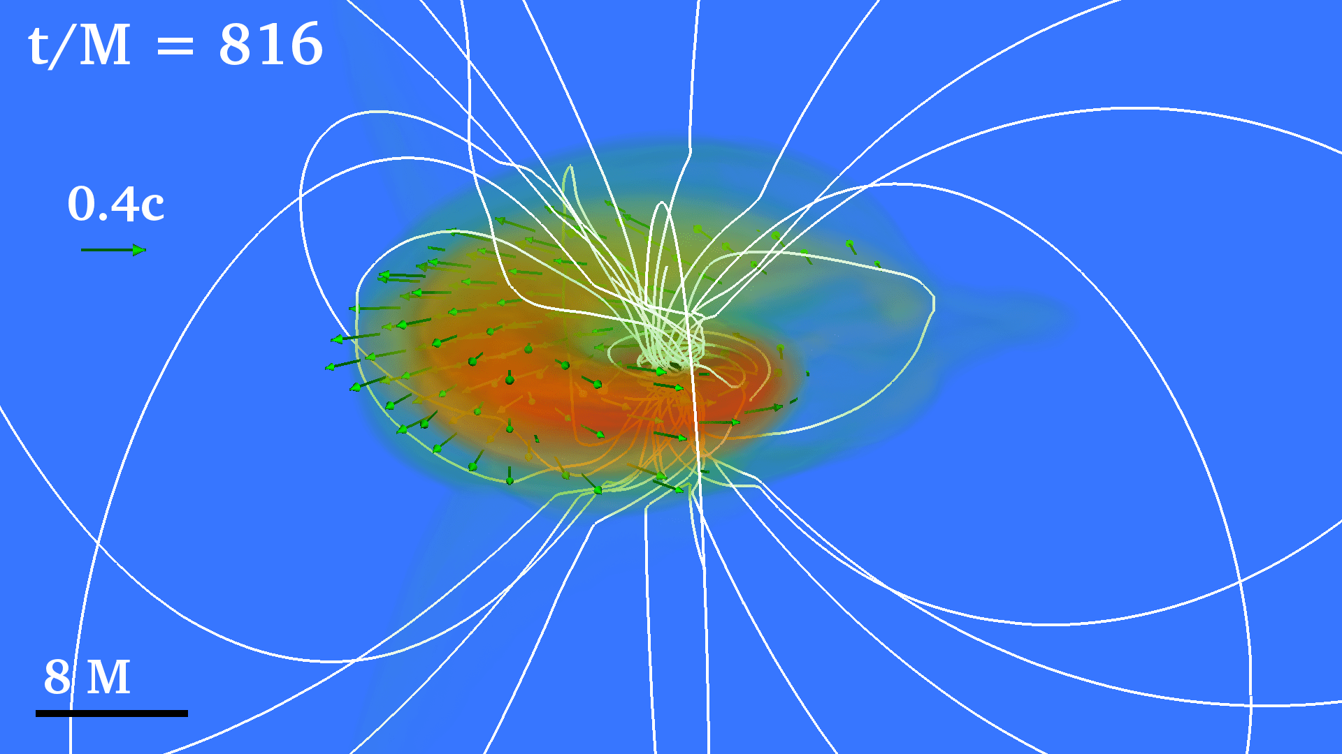
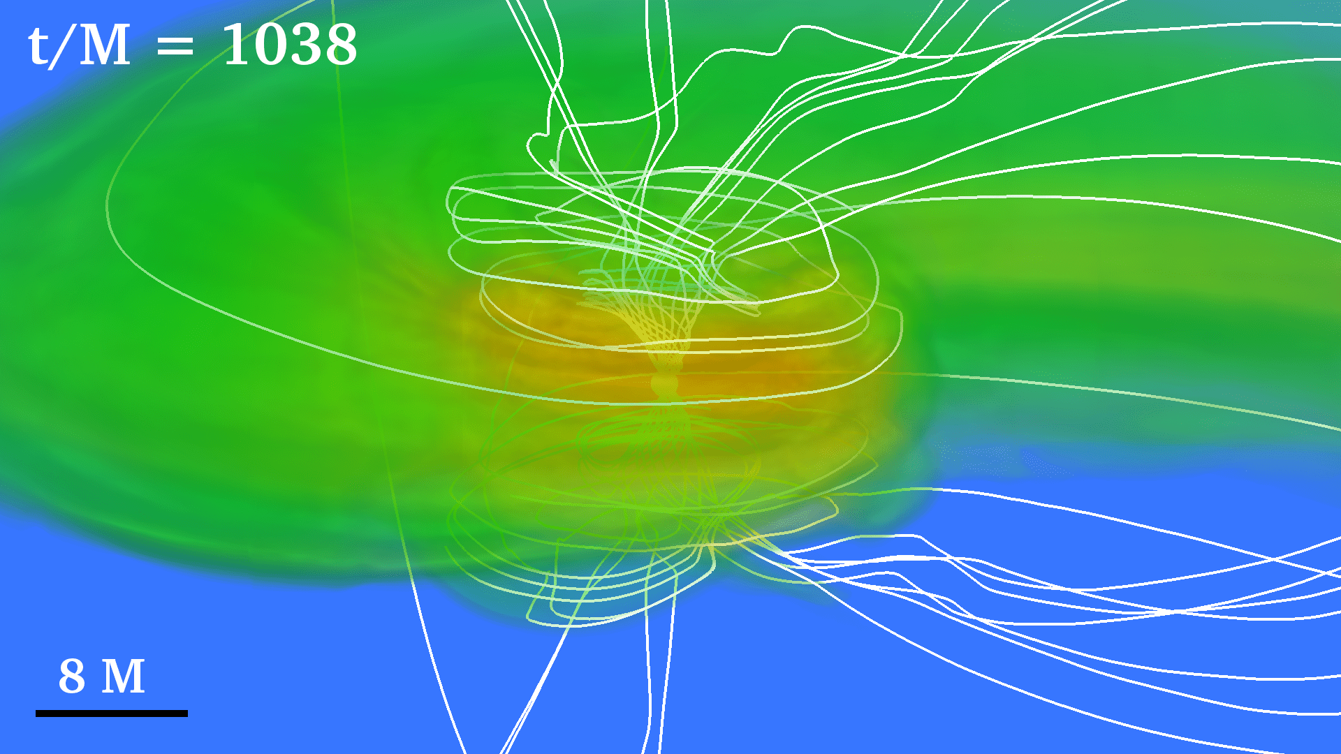
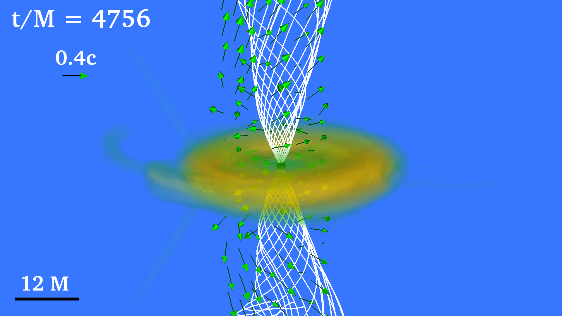
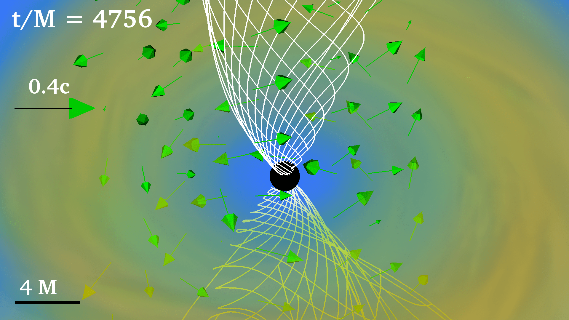
Figure 1: Volume rendering of rest-mass density $\rho_{0}$ normalized to the initial NS maximum value $\rho_{0}=8.92\times 10^{14}\,(1.4M_{\odot}/M_{\rm NS})^{2}\rm{g\,/cm}^{3}$ (log scale) at selected times for case $\rm Aliq3sp0.5$ (see Table 1). White lines denote the magnetic field while the arrows denote the fluid velocity. The BH apparent horizon is shown as a black sphere. Here $M=2.5\times 10^{-2}(M_{\rm NS}/1.4M_{\odot})\rm ms$ = $7.58(M_{\rm NS}/1.4M_{\odot})\rm km$.

II Numerical Methods

The formulation and numerical schemes for BHNS evolutions have been described in detail previously in Etienne et al. (2008, 2012a, 2012b); Paschalidis et al. (2015) and we refer the reader to those references for further details. In this section we introduce our notation and briefly summarize our numerical methods.

II.1 Basic Equations

We carry out the numerical evolution using the Illinois GRMHD moving mesh refinement code that has been embedded in the Cactus/Carpet infrastructure Allen et al. (2001); Cactus ; Schnetter et al. (2004); Carpet . The code has been tested, including resolution studies, and used in the past in multiple GRMHD studies involving compact objects including magnetized BHNS binaries; see e.g. Etienne et al. (2012c, 2012, 2012); Paschalidis et al. (2015). The code has the following sectors:

Spacetime evolution:

We use the $3+1$ formalism of GR and decompose the full metric of the spacetime $g_{\mu\nu}$ according to

$$ds^{2} =g_{\mu\nu}\,dx^{\mu}\,dx^{\nu}$$

$$=-\alpha^{2}\,dt^{2}+\gamma_{ij}\,\left(dx^{i}+\beta^{i}\,dt\right)\left(dx^{j}+\beta^{j}\,dt\right)\,,$$ (1)

with $\alpha$ and $\beta^{i}$ the gauge variables, and $\gamma_{\mu\nu}=g_{\mu\nu}+n_{\mu}\,n_{\nu}$ the three-metric induced on a spatial hypersurface with a timelike future pointing unit vector $n^{\mu}=(1/\alpha,-\beta^{i}/\alpha)$. Associated with the time slice we define the extrinsic curvature $K_{\mu\nu}\equiv-\gamma_{\mu\alpha}\nabla^{\alpha}\,n_{\nu}$. The spatial three-metric and extrinsic curvature are then evolved via the Baumgarte–Shapiro–Shibata–Nakamura (BSSN) formulation Shibata and Nakamura (1995); Baumgarte and Shapiro (1999); see also Baumgarte and Shapiro (2010) for discussion. The dynamical variables are then: (a) the conformal exponent $\phi=\rm{ln}(\gamma)/12$, where $\gamma$ is the determinant of the three-metric, (b) the conformal metric $\tilde{\gamma}_{ij}=e^{-4\phi}\gamma_{ij}$, (c) the conformal, trace-free extrinsic curvature $\tilde{A}_{ij}=e^{-4\phi}(K_{ij}-\gamma_{ij}\,K/3)$, (d) the trace of the extrinsic curvature $K$, and (e) the three auxiliary variables $\tilde{\Gamma}^{i}=-\partial_{j}\tilde{\gamma}^{ij}$. These variables are evolved using the equations of motion (9)-(13) in Etienne et al. (2008), along with the $1+$log time slicing for $\alpha$ and the “Gamma–freezing” condition for $\beta^{i}$ cast in first order form (Eq. (2)-(4) in Etienne et al. (2008)). For numerical stability, we set the damping parameter $\eta$ appearing in the shift condition to $\eta=3.3/M$ for configurations with mass ratio $q=3:1$ and to $\eta=1.2/M$ for the configuration with mass ratio $q=5:1$ (see Table 1). Here $M$ is the Arnowitt-Deser-Misner (ADM) mass of the system.

The spatial discretization is performed by using fourth-order accurate, cell-centered, finite-differencing stencils, except on shift advection terms, where fourth-order accurate upwind stencils are used Etienne et al. (2008). Outgoing wave-like boundary conditions are applied to all the evolved variables. The time integration is performed via the method of lines using a fourth-order accurate, Runge-Kutta integration scheme. Fifth order Kreiss-Oliger dissipation Baker et al. (2006) has been also added in the BSSN evolution equations outside the BH apparent horizon to reduce high-frequency numerical noise.

Table 1: Summary of the initial properties of the BHNS configurations. We list the mass ratio $q\equiv M_{\rm BH}/M_{\rm NS}$, where $M_{\rm BH}$ and $M_{\rm NS}$ are the masses of the BH and NS at infinite separation (see Taniguchi et al. (2006) for details), the dimensionless BH spin parameter $\tilde{a}$, which is either aligned or anti-aligned with respect to the total angular momentum of the system, the dimensionless ADM mass $\bar{M}\equiv\kappa^{-1/2}\,M$ (here $k$ is the polytropic gas constant) and ADM angular momentum $J$ of the binary system, the orbital angular velocity $\Omega_{0}$, and a rough estimate of the innermost stable circular orbit (ISCO) separation $R_{\rm ISCO}$ computed via Eq. (2.21) in Bardeen et al. (1972). All the NSs in the configurations have a nondimensional rest-mass ${\bar{M}_{\rm NS}}=0.15$. The label for each configuration includes successively: a magnetic field configuration tag (Ali=aligned or Til=tilted), a tag identifying the binary mass ratio ($q=3$ or $q=5$), and a tag identifying the spin direction (sp=aligned and sm-antialigned) and the magnitude of the BH spin. In all cases, the initial $M\,\Omega_{0}$ corresponds to an orbital separation of about $D_{0}\simeq 8.7M$.

Model	$q$	$\tilde{a}$	$\bar{M}$	$J/M^{2}$	$M\,\Omega_{0}$	$R_{\rm ISCO}/M_{\rm BH}$
Tilq3sp0.75	3	0.75	0.55	1.09	0.0328	3.2
Aliq3sp0.5	3	0.5	0.55	0.96	0.0330	4.2
Aliq3sp0.0	3	0.0	0.55	0.70	0.0333	6.0
Aliq3sm0.5	3	-0.5	0.55	0.44	0.0338	7.5
Aliq5sp0.0	5	0.0	0.83	0.52	0.0333	6.0

MHD evolution:

For the matter and magnetic field, the Illinois code solves the equations of ideal GRMHD in a conservative scheme via high-resolution shock capturing methods. For that it adopts the conservative variables

$$\rho_{*} \equiv -\sqrt{\gamma}\,\rho_{0}\,n_{\mu}\,u^{\mu}\,,\,\,\,\,\,\tilde{\tau}\equiv\sqrt{\gamma}\,T_{\mu\nu}\,n^{\mu}\,n^{\nu}-\rho_{*}\,,$$

$$\tilde{S}_{i} \equiv -\sqrt{\gamma}\,T_{\mu\nu}\,n^{\mu}\,\gamma^{\nu}_{i}\,,$$

with $T_{\mu\nu}$ the stress-energy tensor for a magnetized plasma defined as

$$T_{\mu\nu}=(\rho_{0}\,h+b^{2})\,u_{\mu}\,u_{\nu}+\left(P+\frac{b^{2}}{2}\right)\,g_{\mu\nu}-b_{\mu}\,b_{\nu}\,,$$

where $\rho_{0}$ is the rest-mass density, $P$ is the pressure, $h=1+\epsilon+P/\rho_{0}$ the specific enthalpy, $\epsilon$ is the specific internal energy, $b^{\mu}=B^{\mu}_{(u)}/(4\,\pi)^{1/2}$ gives the magnetic field as measured by an observer co-moving with the fluid, $b^{2}=b^{\mu}\,b_{\mu}$ gives the magnetic energy ($b$ is proportional to the magnitude of the magnetic field), and $u^{\mu}$ denotes the four-velocity of the fluid. We evolve the conservative variables through Eqs. (27)-(29) in Etienne et al. (2010). To ensure the magnetic field remains divergenceless during the evolution, we integrate the magnetic induction equation by introducing a vector potential $\mathcal{A}^{\mu}$ (see Eqs. (19)-(20) in Etienne et al. (2010)). As noted before Giacomazzo et al. (2012); Etienne et al. (2010), interpolations performed on the vector potential at refinement boundaries on nested grids can induce spurious magnetic fields. To avoid that, we also adopt the generalized Lorenz gauge Farris et al. (2012) with a damping parameter $\xi\sim 5.5/M$ for configurations with mass ratio $q=3:1$ and to $\xi=6.4/M$ for the configuration with mass ratio $q=5:1$ (see Table 1). Finally, we adopt the $\Gamma$–law EOS $P=(\Gamma-1)\rho_{0}\,\epsilon$, with $\Gamma=2$.

II.2 Initial data

The quasiequilibrium BHNS configurations (see Table 1) are constructed by solving the GR constraint equations in the conformal thin-sandwich (CTS) decomposition, along with the relativistic equations of hydrostatic equilibrium, imposing BH equilibrium boundary conditions as in Cook and Pfeiffer (2004). These CTS initial data correspond to BHNS binaries in a quasicircular orbit with a separation chosen to be outside the tidal disruption radius Taniguchi et al. (2008).

The initial data are calculated using the Lorene spectral numerical libraries Gourgoulhon et al. (2016) employing dimensionless quantities as in Baumgarte and Shapiro (2010) where, for example, the mass $M$ can be rescaled as $\bar{M}=k^{-1}\,M$, the spatial coordinates as $\bar{x}^{i}=k^{-1}\,x^{i}$, etc, where $k$ is the polytropic gas constant. The excised BH region is populated with smooth junk data using the technique described in Etienne et al. (2007). As in the previous studies Etienne et al. (2008, 2012a), the initial data quantities are extrapolated from the BH exterior into the interior using a $7^{th}$ order polynomial with a uniform stencil spacing of $\Delta r\approx 0.3\,R_{\rm BH}$, with $R_{\rm BH}$ the radius of the apparent horizon. A detailed description of our methods can be found in Taniguchi et al. (2008); Etienne et al. (2008).

We assume that the initial NS can be modeled as an irrotational $\Gamma=2$ polytrope, and treat BHs that are nonspinning ($\tilde{a}=0$), aligned ($\tilde{a}=0.5$ and $0.75$) and anti-aligned ($\tilde{a}=-0.5$) with respect to the total orbital angular momentum of the system. The mass ratio considered here ranges from $q=3:1$ to $q=5:1$ (see Table 1). In all BHNS cases considered here the resulting NS has a compaction of ${\cal C}={\mathcal{M}}_{\rm NS}/R_{\rm NS}=0.145$, where $\mathcal{M}_{\rm NS}$ and $R_{\rm NS}$ are the ADM mass and the circumferential radius of the NS in isolation. For the adopted EOS the maximum mass configuration has $\mathcal{C}=0.215$. We rescale the rest mass of the star as $M_{\rm NS}=1.4M_{\odot}(k/189.96\rm km^{2})^{1/2}$. For an isolated NS with compaction ${\cal C}={\mathcal{M}}_{\rm NS}/R_{\rm NS}=0.145$, the ADM mass turns out to be $\mathcal{M}_{\rm NS}=1.30(M_{\rm NS}/1.4M_{\odot})M_{\odot}$, the isotropic radius is $R_{\rm iso}=11.2(M_{\rm NS}/1.4M_{\odot})\rm km$ and the Schwarzschild radius is $R_{\rm NS}=13.2(M_{\rm NS}/1.4M_{\odot})\rm{km}$. The maximum rest-mass density of the NS is $\rho_{0,\rm max}=8.92\times 10^{14}\,(1.4M_{\odot}/M_{\rm NS})^{2}\rm g/cm^{3}$. In all our BHNS configurations, the initial orbital angular velocity $M\,\Omega_{0}$ corresponds to an orbital separation of about $D_{0}\approx 8.72M\sim 67.15(M_{\rm NS}/1.4M_{\odot})\rm km$ for configurations with mass ratio $q=3:1$, and $D_{0}\approx 8.68M\sim 101.35(M_{\rm NS}/1.4M_{\odot})\rm km$ for mass ratio $q=5:1$. Note that these BHNS configurations have been used in Etienne et al. (2008, 2012a).

Table 2: Grid hierarchy for models listed in Table 1. Symmetry about the orbital plane (i.e. $z=0$) is imposed in all cases except in $\rm Tilq3sp0.75$ ($90^{o}$–tilted magnetic field) where we consider full 3D domain. The computational mesh consists of two sets of nested refinement boxes, one centered on the BH and the other on the NS. The finest box around the BH (NS) has a half length of $\sim 1.5\,R_{\rm BH}\,(1.2\,R_{\rm NS})$, where $R_{\rm BH}\,(R_{\rm NS})$ is the initial radius of the BH (NS). The number of grid points covering the radius of the BH apparent horizon and the equatorial radius of NS is denoted by $N_{AH}$ and $N_{\rm NS}$, respectively. Note that the resolution used here matches that in Paper I, but it is higher than that in Etienne et al. (2008, 2012a) where the same cases were evolved.

Model	Grid Hierarchy (in units of $M$)(a)	Max. resolution	$N_{\rm AH}$	$N_{\rm NS}$
Tilq3sp0.75	(211.3, 93.0, 46.5, 23.2, 11.6, 5.8, 2.9, 1.45 [1.65], 0.76 [N/A])	$M/60.6$	38	42
Aliq3sp0.5	(253.6, 93.0, 46.5, 23.3, 11.6, 5.8, 2.9, 1.45 [1.65], 0.85 [N/A])	$M/60.6$	35	42
Aliq3sp0.0	(253.6, 93.0, 46.5, 23.3, 11.6, 5.8, 2.9, 1.45 [1.65], 0.96 [N/A])	$M/60.6$	38	42
Aliq3sm0.5	(253.6, 93.0, 46.5, 23.3, 11.6, 5.8, 2.9, 1.45 [1.65], 0.85 [N/A])	$M/60.6$	35	42
Aliq5sp0.0	(196.7, 98.3, 49.2, 24.6, 12.3, 4.4,2.2, 1.1)	$M/48.2$	41	48

^(a) Half length of the refinement boxes centered on both the BH and the NS. When the side around the NS is different, we specify the NS half length in square brackets, or as $\rm[N/A]$ if there is no corresponding refinement box, i.e. if the NS is significantly larger than the BH.

Following Paper I, we evolve the configurations until they reach two orbits prior to tidal disruption. At that point, the NS is endowed with a dynamically unimportant, dipolar magnetic field generated by the vector potential Paschalidis et al. (2013)

$$A_{\phi}=\frac{\pi\,\varpi^{2}\,I_{0}\,r_{0}^{2}}{(r_{0}^{2}+r^{2})^{3/2}}\left[1+\frac{15\,r_{0}^{2}\,(r_{0}^{2}+\varpi^{2})}{8\,(r_{0}^{2}+r^{2})^{2}}\right]\,,$$ (2)

which approximately corresponds to a potential generated by an interior current loop. Here $r_{0}$ is the current loop radius, $I_{0}$ is the current, $r^{2}=\varpi^{2}+z^{2}$, with $\varpi^{2}=(x-x_{\rm NS})^{2}+(y-y_{\rm NS})^{2}$, and $(x_{\rm NS},y_{\rm NS})$ is the position of the center of mass of the NS. As is displayed in Table 1, we consider configurations in which the dipole magnetic moment is either aligned (see left top panel in Fig. 1) or tilted by $90^{o}$ (see left panel in Fig. 2) with respect to the total orbital angular momentum of the system.

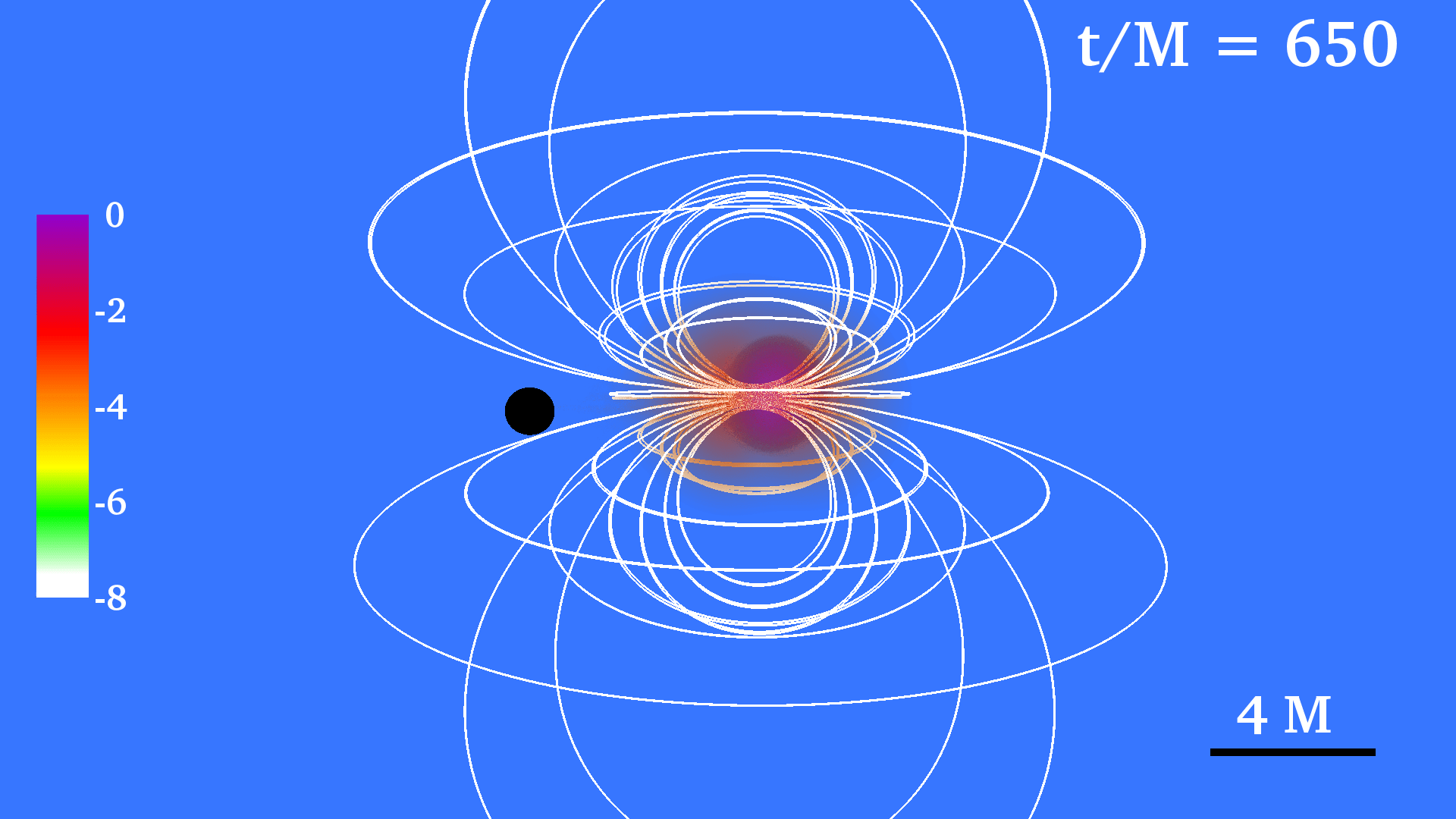
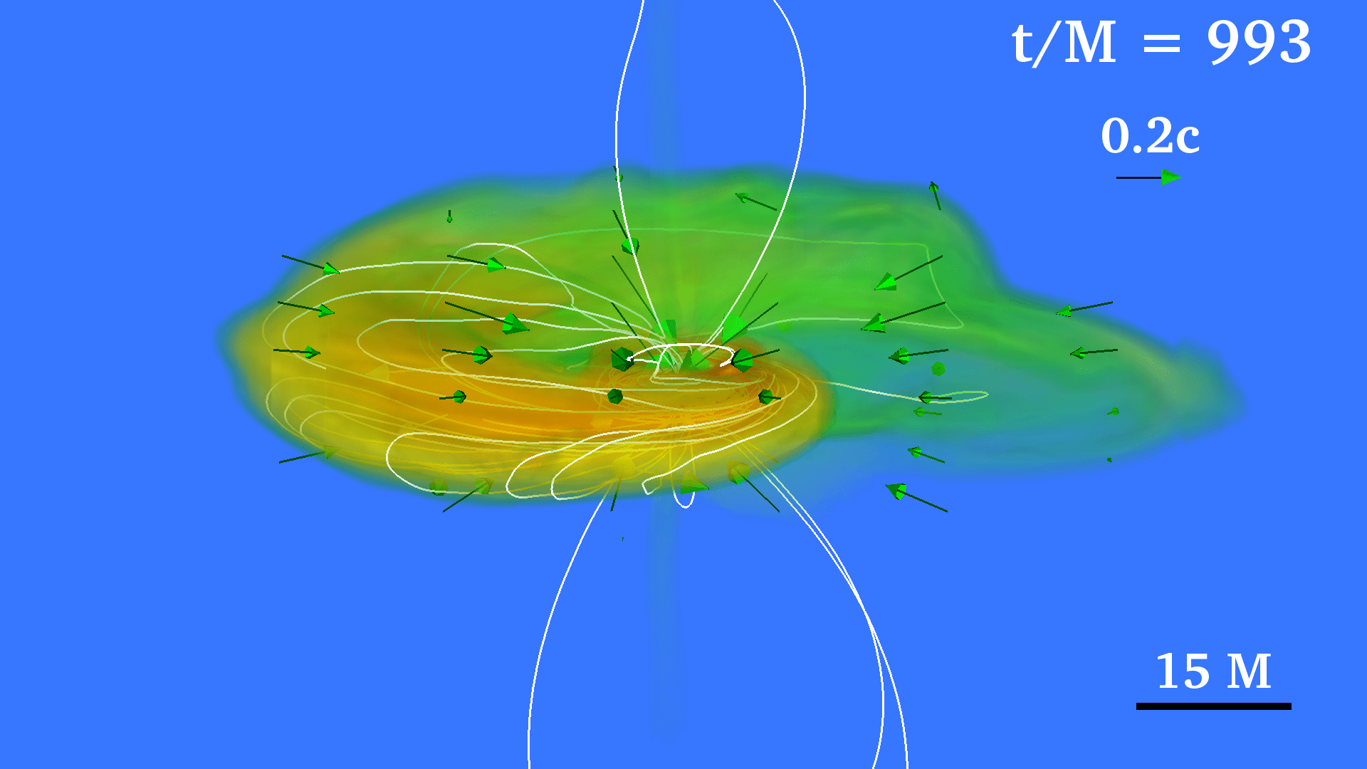
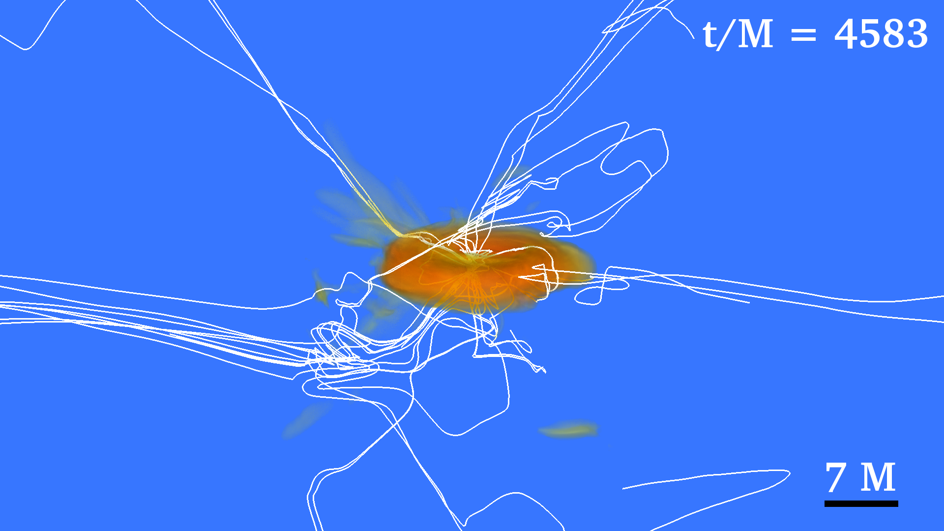
Figure 2: Volume rendering of rest-mass density $\rho_{0}$ normalized to its initial NS maximum value $\rho_{0}=8.92\times 10^{14}\,(1.4M_{\odot}/M_{\rm NS})^{2}\rm{g/cm}^{3}$ (log scale) at selected times for case $\rm Aliq3sp0.0$ (see Table 1). White lines denote the magnetic field while the arrows denote the fluid velocity. The BH apparent horizon is shown as a black sphere. Here $M=2.5\times 10^{-2}(M_{\rm NS}/1.4M_{\odot}){\rm ms}=7.58(M_{\rm NS}/1.4M_{\odot})\rm km$.

For comparison purposes, we choose the current $I_{0}$ and radius of the loop $r_{0}$ such that the magnetic pressure is $5\%$ of the gas pressure at the center of the NS as in Paper I. The resulting magnetic field strength is $B_{\rm pole}\simeq 6.7\times 10^{15}(1.4M_{\odot}/M_{\rm NS})$G on the surface of the star. Notice that although the resulting magnetic field is large, it is still dynamically unimportant and, as it was shown in Paper I, does not affect the tidal disruption or the merger phases. We expect therefore that the final outcome of the post-merger phase should be approximately independent of the initial magnetic field strength; the amplification of the magnetic field following disruption is mainly due to magnetic winding and the MRI Kiuchi et al. (2015).

To reliably evolve the exterior magnetic field with the Illinois GRMHD code, and at the same time mimic the magnetic-pressure dominant environment that likely characterizes the force-free, pulsar-like exterior magnetosphere at the time the magnetic field is seeded in the NS ($t=t_{B}$), a low and variable density is enforced initially in regions where magnetic field stresses dominate over the fluid pressure gradient. This procedure is typically done in ideal MHD codes to evolve exterior magnetic fields (see e.g. Font (2007)). This “atmosphere” is constructed such that the exterior gas-to-magnetic-pressure ratio (the plasma parameter $\beta$) equals a target value $\beta_{0}\ll 1$ everywhere (see Fig. 3). This choice allows us to automatically define the NS surface as the region where the interior plasma parameter $\beta$ equals $\beta_{0}$ for the first time in moving outward from the center, or equivalently

$$\rho_{0}^{\rm surf}=\left({\frac{\beta_{0}\,b^{2}}{2\,\kappa}}\right)^{1/\Gamma}\ll\rho_{0,c}\,,$$ (3)

with $\Gamma=2$, and $\rho_{0,c}$ the initial NS central density. In the stellar exterior we reset the rest-mass density to $\rho_{0}=\rho_{0}^{\rm surf}$. The profile for $\beta$ both inside the star, where the field is weak, and outside is plotted in Fig. 3. The density outside at $t=t_{B}$ is set to

$$\rho_{0}^{\rm atm}=\left({\frac{\beta_{0}\,b^{2}}{2\,\kappa}}\right)^{1/2}\,,$$ (4)

so that as the magnetic field strength falls from the NS surface as $1/r^{3}$, the above prescription forces $\rho_{0}^{\rm atm}$ to fall as $1/r^{3}$ as well.

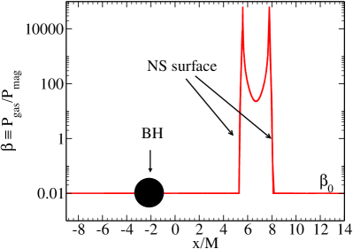
Figure 3: Gas-to-magnetic pressure ratio $\beta\equiv P_{\rm gas}/P_{\rm mag}$ along the x-direction at the time $t=t_{B}$ the dipole-like magnetic field generated by the vector potential $A_{\phi}$ in Eq. 2 is seeded in the star (see Table 1).

In Paper I we showed that different exterior conditions ranging from moderate to complete magnetic field pressure dominance ($\beta_{0}=0.1,\,0.05,\,0.01$) do not affect the final outcome of the BHNS mergers; a larger $\beta_{0}$ affects the inertia of the matter in the atmosphere resulting in a delayed jet launching. We set $\beta_{0}=0.01$ which provides the best approximation to a force-free environment that our code can handle reliably. This choice of $\beta_{0}$ increases total rest-mass of the system in less than $1\%$.

We assume that the pulsar-like magnetosphere comoves with the NS, for which we set the exterior plasma three-velocity to

$$v^{i}=\begin{cases}v^{i}_{\rm CM}\,,&\text{if}\,\,\,\varpi\leq 3\,R_{\rm NS}\,,\\ v^{i}_{\rm CM}\,(3\,R_{\rm NS}/\varpi)^{4}-&\\ \beta^{i}\,(1-(3\,R_{\rm NS}/\varpi)^{4})\,,&\text{if}\,\,\,\varpi>3\,R_{\rm NS}\,,\end{cases}$$ (5)

where $v^{i}_{\rm CM}$ is the three-velocity of the NS centroid. This condition implies that the variable atmosphere is stationary with respect to Eulerian observers.

For the subsequent evolution, we integrate the ideal GRMHD equations everywhere, imposing a density floor in regions where where $\rho_{0}^{\rm atm}<10^{-10}\rho_{0}^{max}$, where $\rho_{0}^{max}$ is the initial maximum density of the NS.

II.3 Grid structure

The grid hierarchy used in our simulations is summarized in Table 2. It consists of two sets of mesh nested refinement boxes centered on both the BH and the NS. We use 9 nested boxes centered on the BH and 8 boxes centered on the NS in configurations with mass ratio $q=3:1$, and 8 nested boxes centered on the BH and on the NS in the configuration with mass ratio $q=5:1$. The finest box has a half length of $\sim 1.5\,R_{\rm BH}$ around the BH and $\sim 1.2\,R_{\rm NS}$ around the NS. These choices resolve the initial apparent horizon equatorial radius by $\gtrsim 70$ grid points, and the initial NS equatorial radius by $\gtrsim 84$ grid points. We impose reflection symmetry across the orbital plane ($z=0$) for all configurations for which the magnetic dipole moment is aligned with the orbital angular momentum of the system, and consider the full 3D domain for the $90^{o}$–tilted magnetic field (see Table 1). Note that the resolution employed here matches the one used in Paper I, and it is higher than that previously employed in Etienne et al. (2008, 2012a) where same cases were evolved.

Table 3: Summary of main results. Here $\tilde{a}$ is the dimensionless remnant BH spin parameter, $\Delta E_{\rm GW}$ and $\Delta J_{\rm GW}$ are the total energy and angular momentum carried away by GWs, respectively. The kick velocity due to recoil is denoted by $v_{\rm kick}$ in $\rm km/s$, $b^{2}/(2\rho_{0})_{\rm ave}$ is the space-averaged value of the magnetic-to-rest-mass-density ratio (force-free parameter) over all the grid points inside a cubical region of length $2R_{\rm BH}$ above the BH pole (see Fig. 8), $B_{\rm rms}$ denotes the rms value of the magnetic field above the BH poles in units of $(1.4M_{\odot}/M_{\rm NS})$G, $\alpha_{SS}$ is the Shakura–Sunyaev viscosity parameter, $M_{\rm disk}$ is the rest-mass of the accretion disk remnant, $\dot{M}$ is the rest-mass accretion rate computed via Eq. (A11) in Farris et al. (2010), $\tau_{\rm disk}\sim M_{\rm disk}/\dot{M}$ is the disk lifetime (lifetime of the jet, if any) in units of $(M_{\rm NS}/1.4M_{\odot})$s, and $L_{\rm jet}$ is the Poynting luminosity in units of $\rm erg/s$ driven by the incipient jet, time-averaged over the last $500M\sim 12.5(M_{\rm NS}/1.4M_{\odot})\rm ms$ of the evolution. A dash denotes “no information available”.

Model	$\tilde{a}$	$\Delta E_{\rm GW}/M_{\rm ADM}$	$\Delta J_{\rm GW}/J_{\rm ADM}$	$v_{\rm kick}$	$b^{2}/(2\rho_{0})_{\rm ave}$	$B_{\rm rms}$	$\alpha_{SS}$	$M_{\rm disk}/{M_{\rm NS}}$	$\dot{M}(M_{\odot}/s)$	$\tau_{\rm disk}$	$L_{\rm jet}$
Aliq3sp0.75(a)	0.85	$0.97\%$	$14.25\%$	54.20	$\gtrsim 100$	$\gtrsim 10^{15.0}$	$0.01-0.03$	$10.0\%$	0.25	$0.5$	$10^{51.2}$
Tilq3sp0.75	0.85	$1.0\%$	$14.33\%$	54.34	0.26	$10^{14.1}$	$0.01-0.013$	$11.29\%$	0.29	$0.54$	$-$
Aliq3sp0.5	0.76	$0.96\%$	$14.95\%$	65.32	113.7	$10^{15.5}$	$0.012-0.031$	$6.15\%$	0.12	$0.71$	$10^{51.6}$
Aliq3sp0.0	0.54	$1.0\%$	$18.38\%$	45.20	3.25	$10^{14.6}$	$0.013-0.022$	$2.33\%$	0.09	$0.36$	$-$
Aliq3sm0.5	0.33	$0.99\%$	$24.96\%$	56.65	$10^{-3}$	$10^{13.3}$	$-$	$0.24\%$	0.03	$0.11$	$-$
Aliq5sp0.0	0.41	$0.91\%$	$19.63\%$	69.96	$10^{-3}$	$10^{12.3}$	$-$	$0.34\%$	0.04	$0.12$	$-$

^(a) BHNS configuration reported in paper I for $\beta_{0}=0.01$.

II.4 Diagnostic quantities

During the numerical integration we adopt a number of diagnostics to analyze and verify the reliability of our magnetized BHNS mergers. We monitor the $L_{2}$ normalized Hamiltonian and momentum constraints computed via Eqs. (40)-(41) in Etienne et al. (2008). In all cases listed in Table 1, we find that the constraint violations peak at $\lesssim 2.7\%$ during the merger, as expected. During inspiral and post-merger phases, the violations are smaller than $\lesssim 1\%$, and stay roughly constant until the end of the evolution. The BH apparent horizon is located and monitored through the AHFinderDirect thorn Thornburg (2004). We estimate the BH mass $M_{\text{\rm BH}}$ and the BH dimensionless spin parameter $\tilde{a}$ via Eqs. (5.2)-(5.3) in Alcubierre et al. (2005). We monitor the conservation of both the total mass $M_{\rm int}$ and the total angular momentum $J_{\rm int}$ interior to a large radius $r$, which coincide with the ADM mass and ADM angular momentum of the system at $r=\infty$, via Eqs. (19)-(22) in Etienne et al. (2012a). To measure the flux of energy and angular momentum carried away by GWs, we use a modified version of the Psikadelia thorn that computes the Weyl scalar $\Psi_{4}$, which is decomposed into $s=-2$ spin-weighted spherical harmonics Ruiz et al. (2008) at different radii between $r_{\rm min}\approx 22M\sim 166(M_{\rm NS}/1.4M_{\odot})\rm km$ and $r_{\rm max}\approx 130M\sim 985(M_{\rm NS}/1.4M_{\odot})\rm km$ for cases with mass ratio $q=3:1$, and $r_{\rm min}\approx 22M\sim 252(M_{\rm NS}/1.4M_{\odot})$km, and $r_{\rm max}\approx 130M\sim 1490(M_{\rm NS}/1.4M_{\odot})\rm km$ for the mass ratio $q=5:1$. We find that $\sim 1.0\%$ of the total energy of our BHNS models is radiated away during the evolution in form of gravitational radiation, while between $\sim 14\%$ and $\sim 25\%$ of the angular momentum is radiated (see Table 3). Taking into account the GW radiation losses, we also find that, in all configurations considered here, the violation of the conservation of $M_{\rm int}$ is $\lesssim 1\%$ along the whole evolution, while the violation of the conservation of $J_{\rm int}$ is $\sim 1\%$ in cases $\rm Aliq3sm0.5$ and $\rm Aliq5sp0.0$ (see Table 1), and $\lesssim 4\%$ in the remaining cases.

In addition, we monitor the conservation of the rest-mass $M_{\rm NS}=\int\rho_{*}d^{3}x$, where $\rho_{*}\equiv\sqrt{\gamma}\rho_{0}\,n_{\mu}\,u^{\mu}$, as well as the magnetic energy growth outside the BH apparent horizon through

$$\mathcal{M}=\int u^{\mu}u^{\nu}T^{(EM)}_{\mu\nu}\,dV\,,$$ (6)

as measured by a comoving observer Etienne et al. (2012a), where $dV=e^{6\phi}\,d^{3}x$ is the proper volume element on the spatial slice. Here $T^{(EM)}_{\mu\nu}$ is the electromagnetic energy-momentum tensor. The rest-mass accretion rate is computed via mass fluxes across the apparent horizon as

$$\dot{M}=-\int_{\rm AH}\alpha\,\sqrt{\gamma}\,\rho_{0}\,u^{\mu}\partial_{\mu}f\,J\,d\theta\,d\phi\,,$$ (7)

where

$$f = \sqrt{(x-x_{h}(t))^{2}+(y-y_{h}(t))^{2}+(z-z_{h}(t))^{2}}$$ (8)

$$- R(t,\theta,\phi)\,,$$

is a scalar function such that $f=0$ on the spatial hypersurface corresponding to the world tube of the BH apparent horizon. Here $J=\partial(f,\theta,\phi)/\partial(x,y,z)$ is the Jacobian, $(x_{h},y_{h},z_{h})$ is the position of the BH centroid, and $R(t,\theta,\phi)$ represents the coordinate distance from the BH centroid to the apparent horizon along the $(\theta,\phi)$ direction. For details see Appendix A in Farris et al. (2010).

To probe MHD turbulence in our systems, we compute the effective Shakura–Sunyaev $\alpha_{\rm SS}$ parameter Shakura and Sunyaev (1973) associated with the effective viscosity due to magnetic stresses through $\alpha_{\rm SS}\sim T^{EM}_{\hat{r}\hat{\phi}}/P$ (see Eq. 26 in Penna et al. (2010)). We also verify that the MRI can be captured in the post-merger phase of our simulations by computing the quality factor $Q_{\rm MRI}\equiv\lambda_{\rm MRI}/dx$, which measures the number of grid points per fastest growing MRI mode. Here $\lambda_{\rm MRI}$ is the fastest-growing MRI wavelength defined as Etienne et al. (2012)

$$\lambda_{\rm MRI}\approx 2\,\pi\,\frac{\sqrt{|b_{P}b^{P}|/(b^{2}+\rho_{0}\,h)}}{|\Omega(r,\theta)|},$$ (9)

where $|b^{P}|\equiv\sqrt{b^{2}-b_{\mu}\,(e_{\hat{\phi}})^{\mu}|^{2}}$, and $(e_{\hat{\phi}})^{\mu}$ is the orthonormal vector carried by an observer comoving with the fluid, $\Omega(r,\theta)$ is the angular velocity of the disk remnant, and $dx$ is the local grid spacing. Typically to capture MRI requires $Q_{\rm MRI}\gtrsim 10$ (see e.g. Sano et al. (2004); Shiokawa et al. (2012)). Finally, we compute the outgoing EM Poynting luminosity

$$L=-\int T^{r(EM)}_{t}\,\sqrt{-g}\,d\mathcal{S}\,,$$ (10)

across spherical surfaces of coordinate radii between $R_{\rm ext}=46M\simeq 350(M_{\rm NS}/1.4M_{\odot})$km and $190M\simeq 1440(M_{\rm NS}/1.4M_{\odot})$km.

III Results

As all our initial BHNS binaries are in a quasicircular orbit with an initial coordinate separation outside the tidal disruption distance, their evolution can be roughly characterized by three stages: late inspiral, tidal disruption-and-merger, and post-merger. During the late inspiral, the orbital separation decreases as energy and angular momentum are carried off by gravitational radiation. Once the NS is disrupted a rapid redistribution of the angular momentum in the external layers of the star pushes matter out of the innermost stable circular orbit (ISCO) causing long tidal tails (see right top and left middle panels in Fig. 1). Depending on the specific angular momentum of the matter in the tidal tail, it can be accreted, it can wrap around the BH to form the accretion disk (see left middle panel in Fig. 1), or it can be dumped in the atmosphere as escaping or fall-back debris.

The fluid motion in the new-born disk drags the frozen-in magnetic field lines into a predominantly toroidal configuration. However, the presence of an external magnetic field in the initial NS that connects matter in the star with footpoints at the poles of the BH establishes a poloidal field component that persists throughout the disk and amplifies following tidal disruption (see second row in Fig. 1 and central panel in Fig. 2). Depending on the poloidal magnetic field, the fall-back debris, and the rest-mass of the disk, these instabilities may induce high magnetic pressure gradients above the BH poles that eventually can launch an outflow. In paper I, we showed for the first time that BHNS remnants with a strong poloidal magnetic field component can launch a collimated, mildly relativistic outflow—an incipient jet– and hence be the progenitors of sGRBs. In the following section, we summarize the dynamics of our new BHNS configurations that differ in BH spin, mass ratio, and magnetic field configuration (see Table 1). Table 3 highlights the key parameters at the termination of our simulations.

III.1 Effect of black hole spin

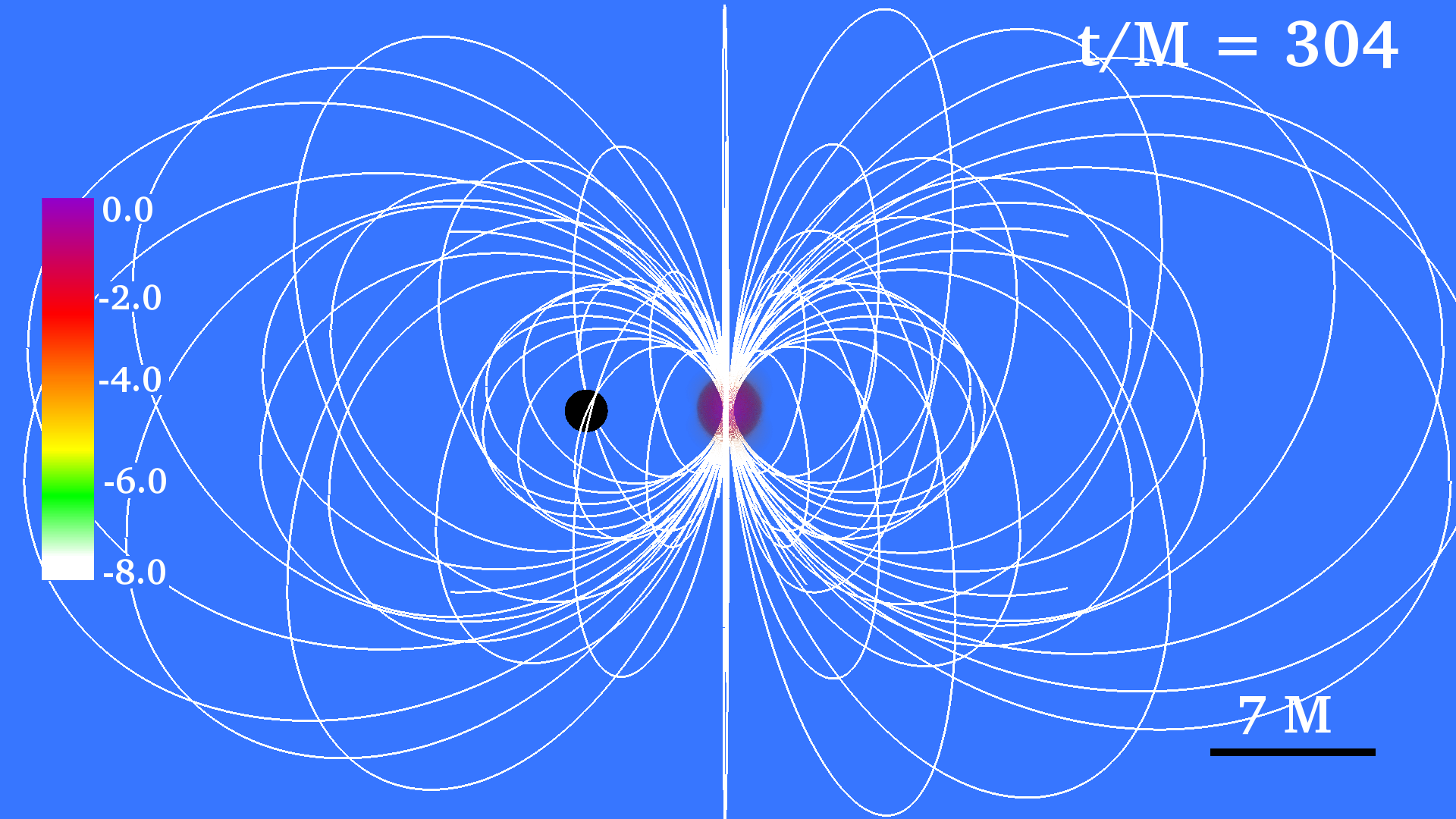
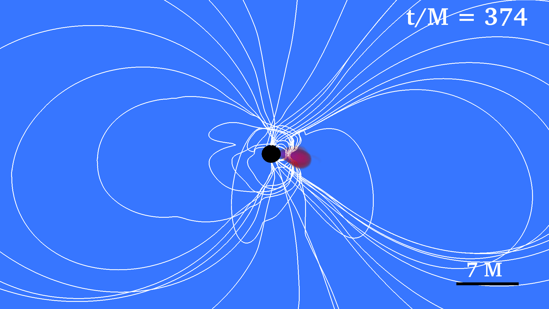
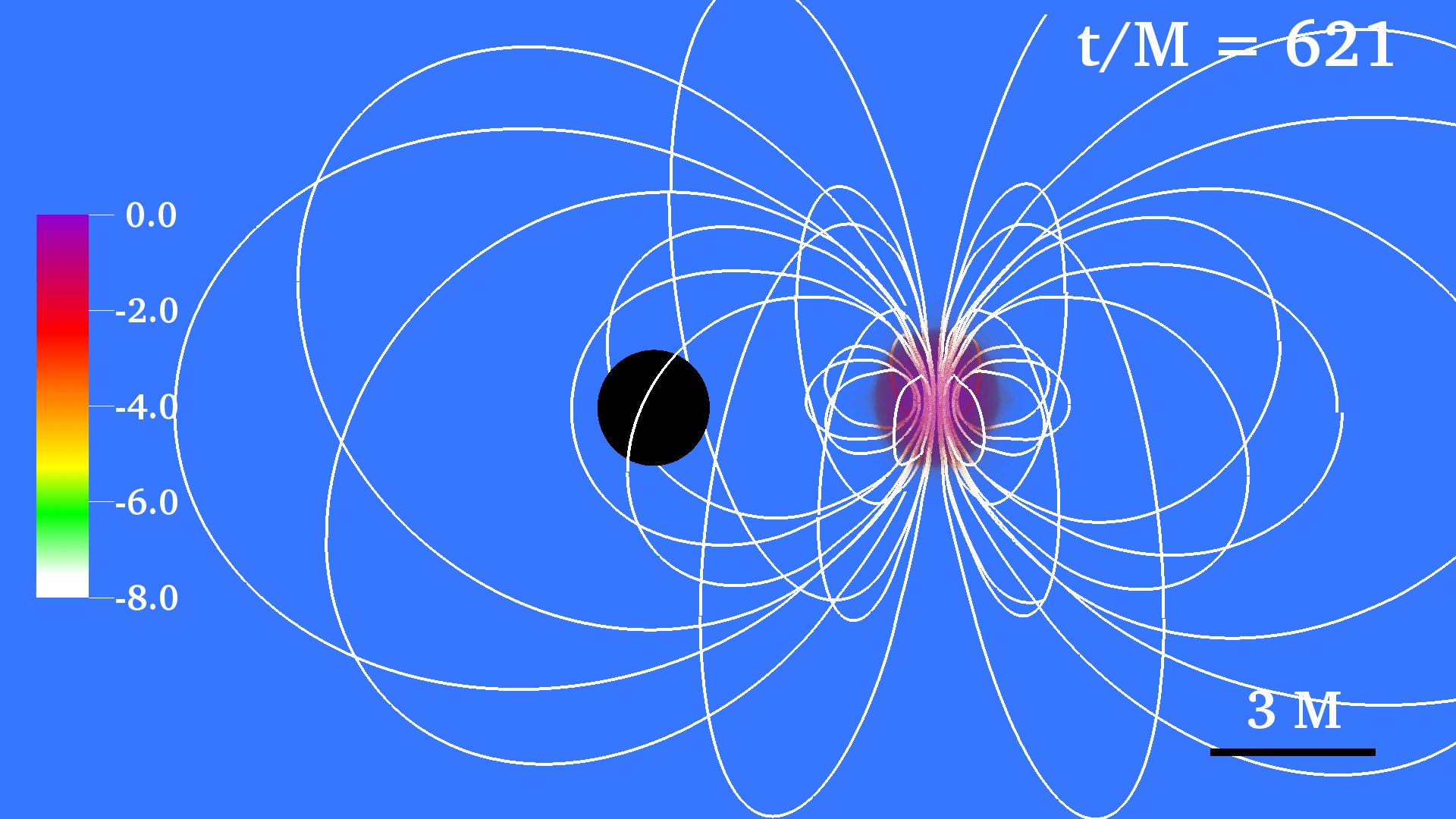
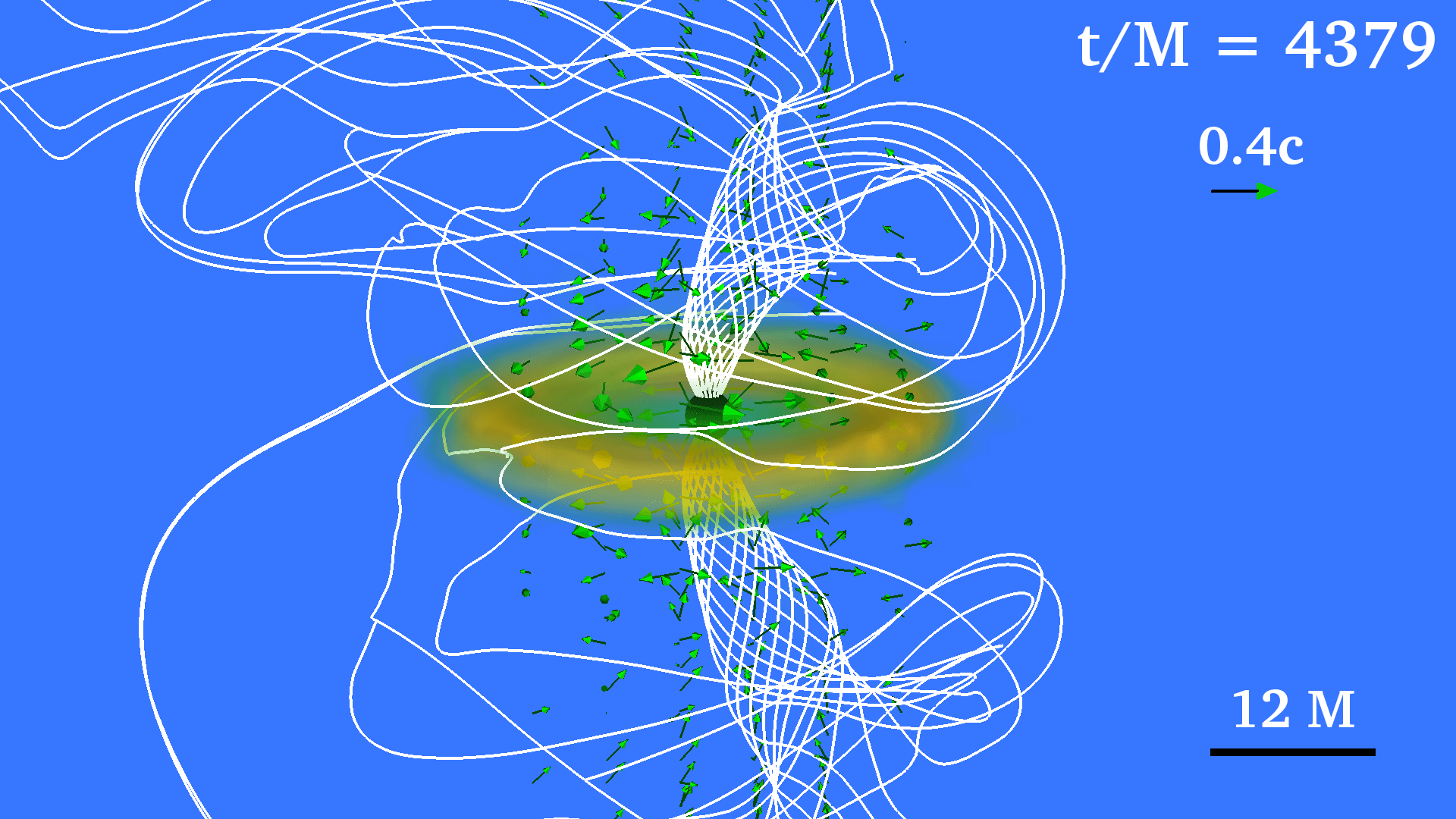
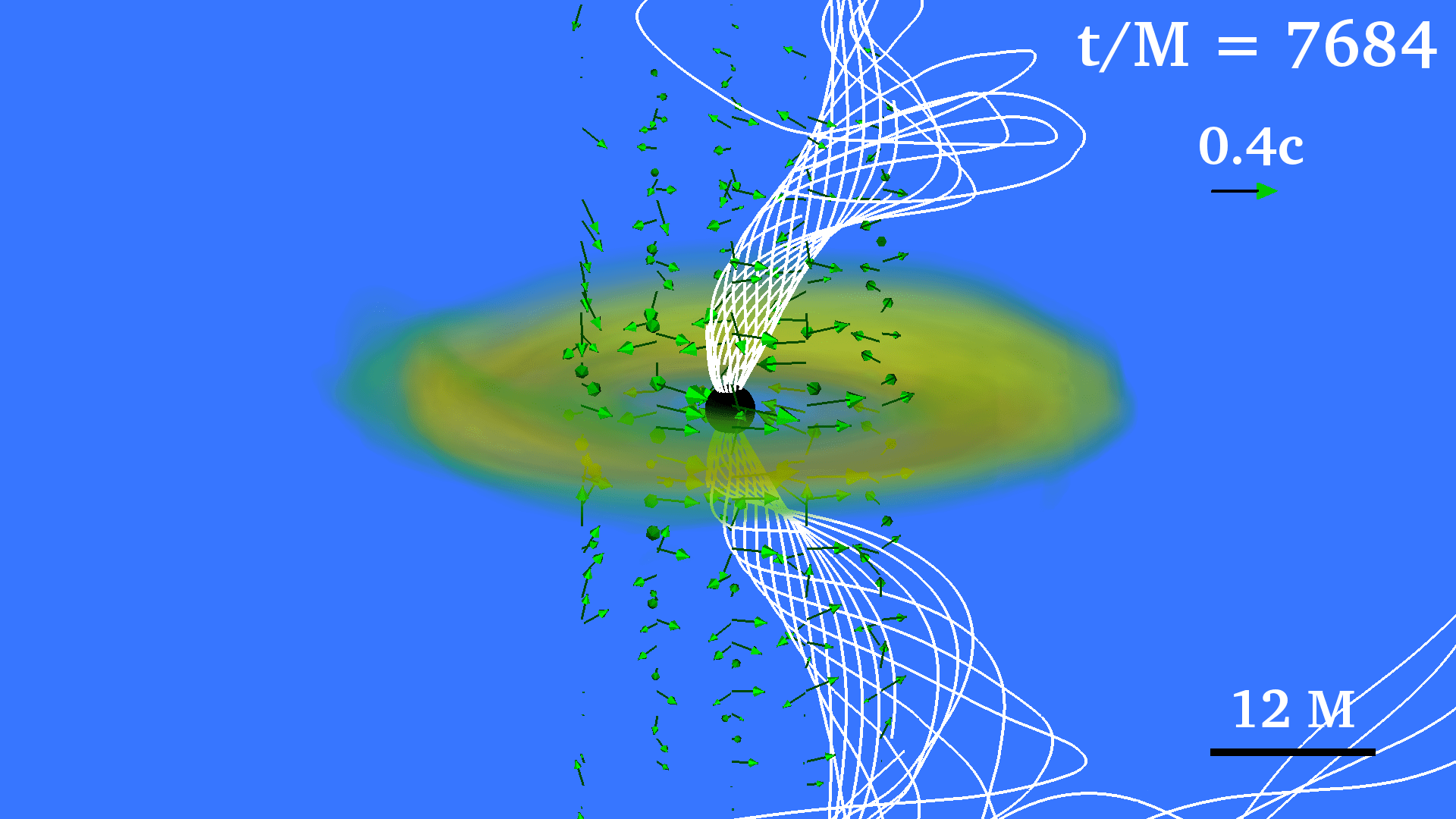
Figure 4: Volume rendering of rest-mass density $\rho_{0}$ normalized to its initial NS maximum value $\rho_{0}=8.92\times 10^{14}\,(1.4M_{\odot}/M_{\rm NS})^{2}\rm{g/cm}^{3}$ (log scale) for cases Aliq3sm0.5 (top row) and Aliq3sp0.0 (bottom row) at selected times. White lines denote the magnetic field while the arrows denote the fluid velocity. The BH apparent horizon is shown as a black sphere. Here $M=2.5\times 10^{-2}(M_{\rm NS}/1.4M_{\odot})\rm ms$= $7.58(M_{\rm NS}/1.4M_{\odot})\rm km$. 

To disentangle the effects of the initial BH spin $\tilde{a}$ on jet launching from the effects of the mass ratio and the magnetic field geometry, we next consider only configurations with mass ratio $q=3:1$, aligned magnetic field and BH spin $\tilde{a}=-0.5,\,0.0,\,0.5$. For comparison, we also summarize the results of the configuration reported in Paper I that corresponds to a similar configuration but with a BH spin $\tilde{a}=0.75$.

Figs. 1 and 4 (see also Fig. 1 in Paper I) display snapshots of the evolution of the rest-mass density along with the magnetic field lines starting from magnetic field insertion at $t=t_{B}$, followed by the disruption of the star and the formation of the accretion disk. The bulk of the star is accreted into the BH, and the disk + BH remnant eventually settles down as does the outflow, when it occurs.

Figure 5: Rest-mass $M_{\rm NS}$ of NS matter outside the BH versus time for all cases listed in Table 1. The time has been shifted by $t_{B}$, at which time the magnetic field is seeded in the NS.

Consider the binary separation at which the star is tidally disrupted. It can be estimated by (see Eq. (17.19) in Baumgarte and Shapiro (2010))

$$R_{\rm tid}\simeq 2.4\,q^{-2/3}\,\mathcal{C}^{-1}\,M_{\rm BH}\,.$$ (11)

For a star with compaction $\mathcal{C}=0.145$ and mass ratio $q=3:1$ we find that disruption distance is $R_{\rm tid}\simeq 8.0M_{\rm BH}$. On the other hand, we estimate the initial position of the ISCO using Eq. (2.21) in Bardeen et al. (1972), which is strictly correct for a test particle in a Kerr spacetime (see Taniguchi et al. (2008) for a careful analysis). We find that the ISCO ranges from $R_{\rm ISCO}\sim 7.5M_{\rm BH}$ (for Aliq3sm0.5 case) to $\sim 3.2M_{\rm BH}$ (for Aliq3sp0.75 case). We expect thus heavier disks in configurations with higher spinning BH.

After $t-t_{B}\sim 40M\sim 1(M_{\rm NS}/1.4M_{\odot})$ms following the onset of accretion the bulk of NS in the case Aliq3sm0.5 is quickly swallowed by the BH companion along with its frozen-in magnetic field (see Fig. 5). Only a tiny fraction of tidally disrupted debris (less than $1\%$ of the rest-mass of the NS) is left to form the a disk around a BH remnant with spin $\tilde{a}\sim 0.3$ (see Table 3). The rest-mass accretion rate computed through Eq. 7 settles down to $\dot{M}=8\times 10^{-2}M_{\odot}/s$ by $t-t_{\rm GW}\approx 690M\sim 26(M_{\rm NS}/1.4M_{\odot})\rm ms$ and then decays slowly (see Fig. 6). Here $t_{\rm GW}$ corresponds to the time (retarded) of the peak GW amplitude measured at $r_{\rm ext}\approx 60M\sim 455(M_{\rm NS}/1.4M_{\odot})\rm km$. Fig. 7 shows the evolution of the magnetic energy $\mathcal{M}$ outside the BH horizon. During the first $\sim 40M$ following the onset of the accretion, the magnetic energy plummets by three orders of magnitude (see Table 3), as expected. By the time we terminate the simulation [$t-t_{\rm GW}\sim 3000M\sim 75(M_{\rm NS}/1.4M_{\odot})\rm ms$], we do not find any evidence of an outflow or tightly wound and globally collimated magnetic field (see right top panel in Fig. 4), although we observe that the field lines just above the BH poles have been partially wound into a helical structure within $\sim 2R_{\rm BH}$, due to low density fluid motion. At that time, the rms value of the magnetic field above the BH pole is only $\sim 10^{13.3}(1.4M_{\odot}/M_{\rm NS})\rm G$, which is expected because only the weakly magnetized external layers of the star survive the merger and form the disk and the field is not amplified much during the post-merger phase (see Fig. 8). Not surprisingly, a basic ingredient for jet launching is a sizable remnant accretion disk.

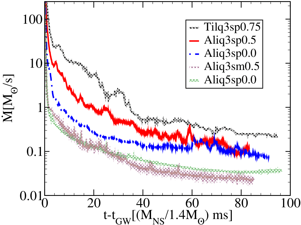
Figure 6: Rest-mass accretion rate for all case listed in Table 1 computed via Eq. (A11) in Farris et al. (2010). Time is measured from the moment (retarded time $t-r$) of maximum GW amplitude $t_{\rm GW}$.

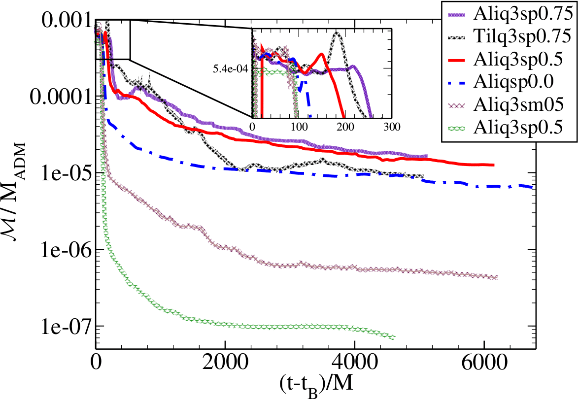
Figure 7: Total magnetic energy $\mathcal{M}$ outside the BH apparent horizon for all cases listed in Table 1, normalized to the ADM mass $M_{\rm ADM}=9.3\times 10^{54}(M_{\rm NS}/1.4M_{\odot})$erg. The inset shows that there is no significant enhancement of $\boldmath\mathcal{M}$ during disruption. The time has been shifted by $t_{B}$ at which moment the magnetic field is seeded in the NS.

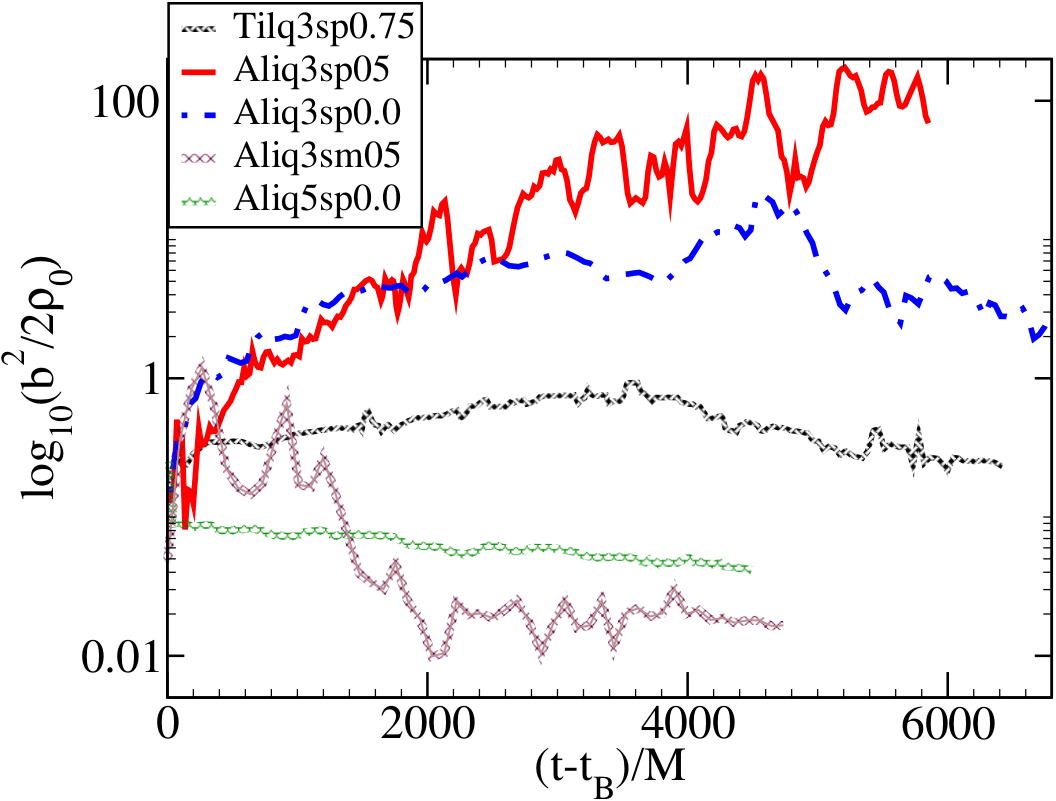
Figure 8: Average value of the force-free parameter $b^{2}/(2\rho_{0})$ vs time (log scale) for all cases listed in Table 1. The average is computed using grid points contained in a cube of edge $2R_{\rm BH}$ above the BH. Here $R_{\rm BH}$ denotes the radius of the BH apparent horizon.

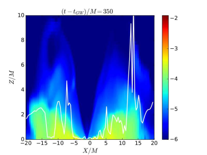
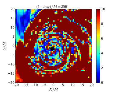
Figure 9: Rest-mass density on the meridional plane along with the $\lambda_{\rm MRI}/2$ (left panel), and the quality factor $Q_{\rm MRI}$ on the equatorial plane (right panel) at $t-t_{\rm GW}\sim 350M\sim 8.75(M_{\rm NS}/1.4M_{\odot})\rm ms$ following the peak GW amplitude in case $\tilde{a}=0.5$ (Aliq3sp0.5) but similar behavior among all cases with spinning BH $\tilde{a}\geq 0$. The BH apparent horizon is denoted by the black disk.

On the other hand, as the BH spin increases the ISCO shrinks, and therefore the NS can be totally disrupted before being swallowed by the BH companion (see right top and left middle panels in Fig. 1). The larger the BH spin, the longer the tidal tails, and thus the heavier the accretion disk (see Table 3). By about $t\sim 1200M\sim 30(M_{\rm NS}/1.4M_{\odot})$ms following the peak of the accretion ($t-t_{B}\sim 300M$), the remnant disk settles with a mass of $\sim 4.43\%$ of the rest-mass of the NS in case Aliq3sp0.0, $\sim 10.1\%$ in case Aliq3sp0.5, and $\sim 15.2\%$ in case Aliq3sp0.75 (see Fig. 5), and then slowly decreases in mass as the accretion proceeds. Similar values were reported in Etienne et al. (2008, 2012a), indicating that the seeded magnetic field has a low impact on the formation of the disk remnant (see Table 3 for values near the end of the simulations).

By $t-t_{\rm GW}\approx 1500M\sim 38(M_{\rm NS}/1.4M_{\odot})$ms, the rest-mass accretion rate in the three cases begins to settle to quasi-equilibrium (see Fig. 6), and then slowly decays (see also Table 3). By the time we terminate the simulations we find that ${\dot{M}}\approx(0.09,\,0.12,\,0.25)M_{\odot}/s$, for cases $\tilde{a}=0.0,\,0.5,\,\rm{and}\,\,0.75$, respectively. The remnant disk is hence expected to be accreted in $\Delta t\sim M_{\rm disk}/\dot{M}\sim 0.36(M_{\rm NS}/1.4M_{\odot})$s for Aliq3sp0.0, in $\Delta t\sim 0.75(M_{\rm NS}/1.4M_{\odot})$s for Aliq3sp0.5, and in $\Delta t\sim 0.5(M_{\rm NS}/1.4M_{\odot})$s for Aliq3sp0.75.

During the tidal disruption and the early disk + BH phase, the frozen-in magnetic field is either stretched and wound into a predominantly toroidal configuration as part of the tidal tail wraps around the BH forming the accretion disk, or stretched by the low density material dumped in the atmosphere in the poloidal direction (see right top and left middle panels in Fig. 1). However, during those phases we do not observe a significant enhancement of the total magnetic energy (see Fig. 7) which is expected since initially the magnetic field has an equipartition–strength [$B_{\rm pole}\simeq 6.7\times 10^{15}(1.4M_{\odot}/M_{\rm NS})$G], i.e. magnetic energy $\approx$ kinetic energy Kiuchi et al. (2015). During $t\sim 40M=1(M_{\rm NS}/1.4M_{\odot})\rm ms$ following the onset of accretion, the bulk of the star, which contains most of the magnetic energy, is swallowed by the BH (see Fig. 5) leaving only $\sim 6\%$ of the total initial $\mathcal{M}$ in case Aliq3sp0.0, and $\sim 15\%$ in Aliq3sp0.05 and Aliq3sp0.75. As the accretion proceeds, the magnetic energy slowly decreases until quasi–stationary equilibrium is achieved.

To probe MHD turbulence in the post-merger phase, we compute the effective Shakura–Sunyaev $\alpha_{\rm SS}$ parameter associated with viscous dissipation due to magnetic stresses. In all our cases we find that, between the ISCO and the position of the maximum value of the rest-mass density, $\alpha_{\rm SS}$ is $\sim 0.01-0.031$ (see Table 3). Similar values for $\alpha_{\rm SS}$ were found in previous MHD studies of accretion disks Krolik and Hawley (2007); Gold et al. (2014). To check if the MRI is indeed operating in the disk + BH remnant, we compute the quality factor $Q_{\rm MRI}$ at $t-t_{\rm GW}\sim 350M\sim 8.75(M_{\rm NS}/1.4M_{\odot})\rm ms$ following the GW peak amplitude. In the three cases, we find that in the bulk of the disk the fastest growing mode of $\lambda_{\rm MRI}$ is resolved by at most five gridpoints (see Fig. 9), although in some parts it is resolved by more than ten. We also find that for the most part $\lambda_{\rm MRI}/2$ fits in the disk. As the timescale for MRI is $\tau_{\rm MRI}\sim\Omega^{-1}\sim 0.1-0.2(M_{\rm NS}/1.4M_{\odot})^{1/2}$ms, it is likely that the MRI is at least partially resolved and operating in the system Gold et al. (2014). Here $\Omega$ is the angular velocity of the disk. The accretion is thus likely driven by MHD turbulence.

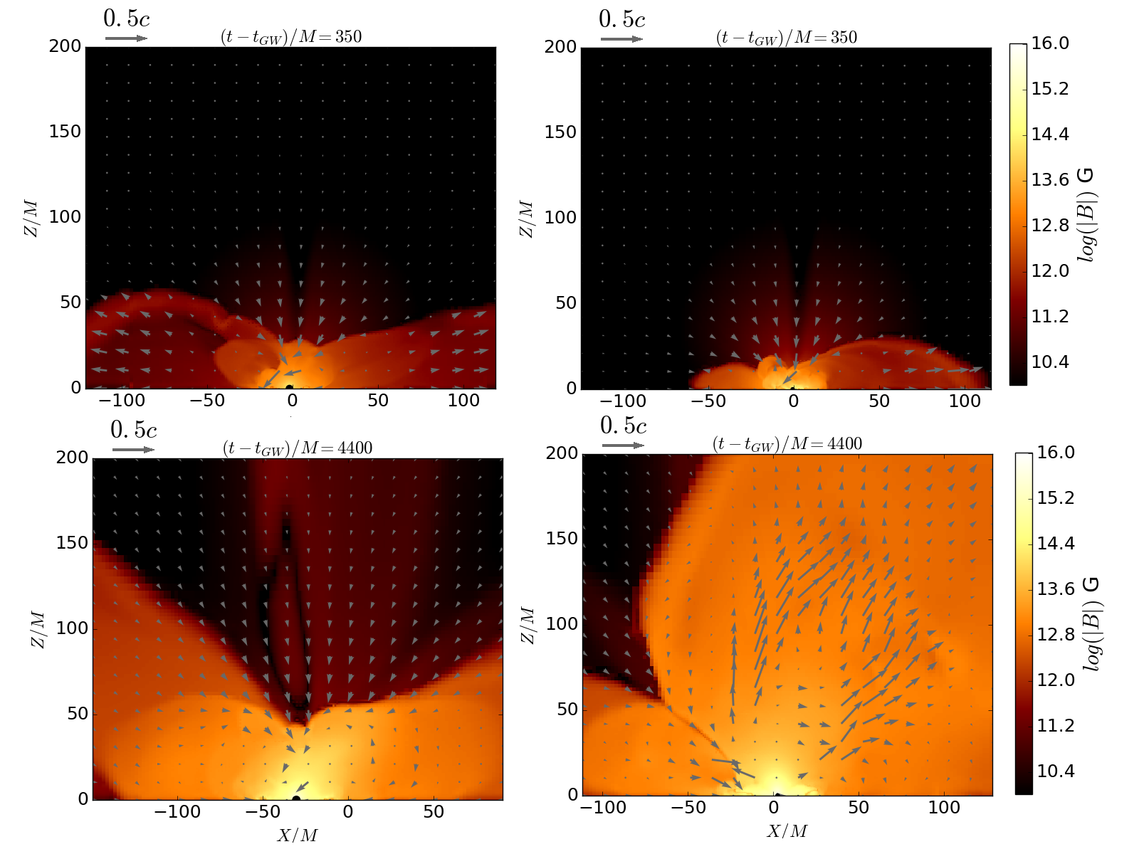
Figure 10: Magnetic field strength on a meridional plane after $t-t_{\rm GW}\sim 350M\sim 8.75(M_{\rm NS}/1.4M_{\odot})\rm ms$ following the maximum GW amplitude, time at which the accretion disk + disk remnant starts to settle, and nearly to the end of the evolution for cases Aliq3sp0.0 (left column) and Aliq3sp0.5 (right column). Arrows denote the fluid velocity, while the BH apparent horizon is shown as a black disk.

Shortly after tidal disruption, the MRI and magnetic winding in the disk convert poloidal to toroidal flux on an Alfvén timescale Shapiro (2000), $\tau_{\rm A}\sim 1.0(B/10^{15}\rm G)^{-1}(R_{\rm disk}/50\rm km)(\rho/10^{14}\rm g/cm^{3})^{1/2}\rm ms$, where $R_{\rm disk}$ is the characteristic radius of the disk (see Eq. (10.6) in Shibata (2015)), building high magnetic pressure gradients above the BH and pushing gas outwards above the BH poles (see top panels in Fig. 10). As the regions above the BH poles are cleared, the environment becomes near force-free ($b^{2}\gg\rho_{0}$). Depending on the initial spin of the BH companion, we find the following:

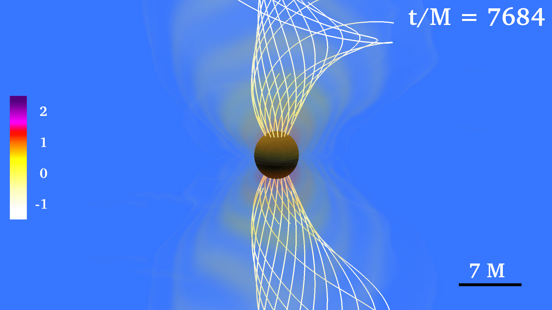
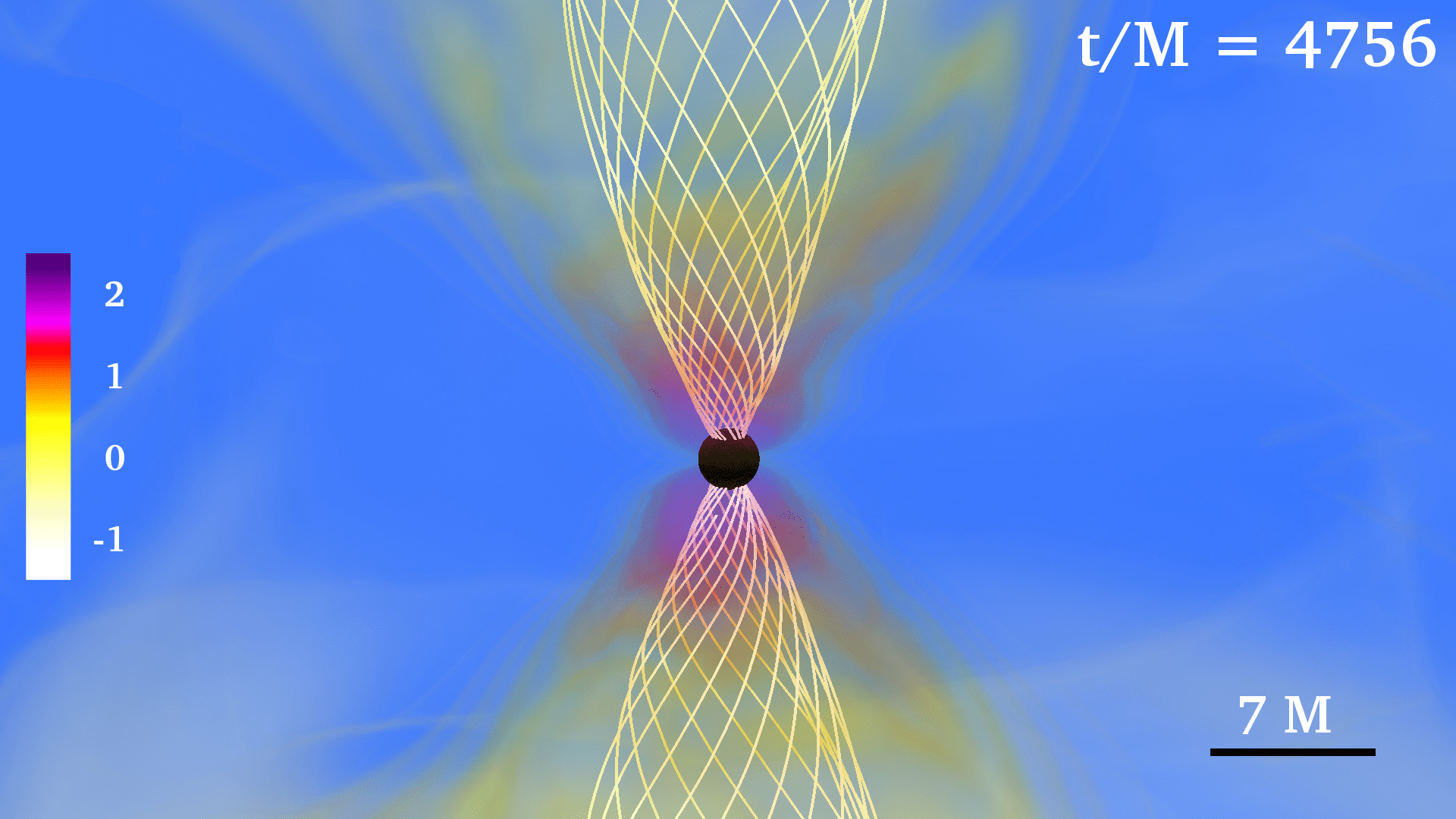
Figure 11: Volume rendering of the ratio $b^{2}/2\rho_{0}$ (log scale) near the end of the simulation for case Aliq3sp0.0 (left panel) and Aliq3sp0.5 (right panel). The magnetic field lines are denoted by white lines plotted in regions where $b^{2}/2\rho_{0}\geq 0$.

Nonspinning (Aliq3sp0.0) case:

By $t-t_{\rm GW}\sim 400M\sim 10(M_{\rm NS}/1.4M_{\odot})\rm ms$, we observe that above the poles of the BH remnant with spin $\tilde{a}\sim 0.54$ (see Table 3) the magnetic field has been wound into a helical funnel (see middle and right bottom panels in Fig. 4) but, in contrast with the Aliq3sp0.75 case reported in Paper I, there is no evidence of a large-scale sustained outflow. As the magnetic pressure above the BH poles increases, magnetically dominated regions ($b^{2}/2\rho_{0}^{2}\gtrsim 1$) expand outwards above the BH poles until the magnetic pressure balances the ram pressure produced by fall-back gas at a height of $\sim 15M\sim 115(M_{\rm NS}/1.4M_{\odot})\rm km$ (see left bottom in Fig. 10). At that height the magnetically dominated regions rise and fall above the BH poles, but no longer expand. The left panel in Fig. 11 shows the magnetically dominated regions along with the field lines near the end of the simulation.

As jet launching via the Blandford–Znajek (BZ) mechanism requires a near force–free environment above the BH poles, we compute the space-averaged value of the force-free parameter $b^{2}/(2\rho_{0})$ on a cubical region of a length side $2\,R_{\rm BH}$ just above the BH poles during the whole evolution (see Fig. 8). We observe that the plasma parameter rapidly grows during the first $t-t_{B}\sim 2000M\sim 50(M_{\rm NS}/1.4M_{\odot})\rm ms$ following the insertion of the magnetic field, and then settles down to $b^{2}/2(\rho_{0})_{|ave}~{}\sim 3$ (see Table 3). After about $t-t_{B}=6000M\sim 150M(M_{\rm NS}/1.4M_{\odot})\rm ms$, near the end of the simulation, a persistent fall-back flow toward the BH is observed; the matter ejected during the disruption has a specific energy $E=-u_{0}-1<0$ (in the asymptotically flat region) and eventually rains down with increasing the ram-pressure. However, we also observe that magnetic field above the BH poles is amplified from $\sim 10^{13.4}(1.4M_{\odot}/M_{\rm NS})$G, when the disk first settles, to $\sim 10^{14.6}(1.4M_{\odot}/M_{\rm NS})$G near the end of the simulation (see Fig. 10). Hence a longer simulation may be needed for a magnetically driven outflow to emerge. However, if the fall-back debris timescale is longer than that of the disk, jet launching may be suppressed. This suggests that there may be a threshold value of the initial BH spin below which a sustained outflow is suppressed.

Spinning (Aliq3sp0.5 and Aliq3sp0.75) cases:

As in the above case, by $t-t_{\rm GW}\sim 400M\sim 10(M_{\rm NS}/1.4M_{\odot})\rm ms$ when the remnant disk + bh first settles (see bottom panel of Fig. 12), the field lines have been wound into a helical funnel (see right top and left middle panels in Fig. 1). However, in contrast to case Aliq3sp0.0, as the accretion above the remnant BH poles proceeds, the atmosphere becomes thinner, and the magnetic pressure gradients grow. Fig. 8 shows that following the magnetic field insertion, the force-parameter $b^{2}/2\rho_{0}$ above the BH poles grows from $\sim 10^{-1}$ to $\gtrsim 100$ (see also right panel in Fig. 11) near the end of the simulation (see Table 3). Eventually the magnetic pressure settles to a value $b^{2}/2\rho_{0}\gtrsim 10$ that allows it to overcome the ram-pressure of the atmosphere. At about $t-t_{\rm GW}\sim 400M\sim 10(M_{\rm NS}/1.4M_{\odot})$ms, the inflow is halted, and a magnetically sustained outflow emerges (see bottom panels in Fig. 1). The unbound outflow ($E=-u_{0}-1>0$) extends to heights greater than $100M\sim 760(M_{\rm NS}/1.4M_{\odot})$km in Aliq3sp0.5 ($\tilde{a}=0.5$) at $t-t_{\rm GW}\sim 3500{\rm M}\sim 88(M_{\rm NS}/1.4M_{\odot})$ms, and at $t-t_{\rm GW}\sim 4000{\rm M}\sim 100(M_{\rm NS}/1.4M_{\odot})$ms in Aliq3sp0.75 ($\tilde{a}=0.75$). The characteristic maximum value of the Lorentz factor in the funnel is $\Gamma_{L}\sim 1.2-1.3$. So, we conclude that by $\gtrsim 88(M_{\rm NS}/1.4M_{\odot})$ms these two cases launch an incipient jet –an unbound and mildly relativistic outflow within a tightly wound, collimated, helical magnetic funnel above the BH poles. The delay of the jet launching in Aliq3sp0.75 with respect to that in Aliq3sp0.5 is likely due to a heavier atmosphere; a larger ejection of the matter outside the ISCO occurs for higher spins. Although the jet is only mildly relativistic, it is expected that the jet will be accelerated to $\Gamma_{L}\gtrsim 100$ as required by sGRB models. As it was pointed out in Paper I, the maximum attainable Lorentz factor of a magnetically–powered, axisymmetric jet is $\Gamma_{L}^{\rm max}\sim b^{2}/2\rho_{0}$ Vlahakis and Königl (2003). The lifetime of the engine fuel (lifetime of the disk) is $\Delta t\sim 0.5-0.75(M_{\rm NS}/1.4M_{\odot})s$ and thus consistent with sGRBs Bhat et al. (2016). We also observe a magnetic field amplification above the BH poles from $\sim 10^{13.4}(1.4M_{\odot}/M_{\rm NS})$G, when the disk first settles, to $\gtrsim 10^{15}(1.4M_{\odot}/M_{\rm NS})$G near the end of the simulation (see right bottom panel in Fig. 10).

The level of collimation of the jet is measured by the funnel opening angle $\theta_{\rm jet}$, which is defined as polar angle at which the Poynting flux drops to $50\%$ of its maximum. Based on the angle distribution of the outgoing flux on the surface of a sphere with coordinate radius $60M\sim 460(M_{\rm NS}/1.4M_{\odot})\rm km$ (see Fig. 13), we estimate that the opening angle of the jet is $\sim 25^{\circ}-30^{\circ}$.

We compute the ejecta via $M_{\rm esc}=\int_{|u_{t}|>1}\rho_{0}d^{3}x$ at different radii between $30M\sim 230(M_{\rm NS}/1.4M_{\odot})\rm km$ and $100M\sim 760(M_{\rm NS}/1.4M_{\odot})\rm km$. We find that in these cases the rest-mass fraction $M_{\rm esc}/M_{NS}$ of the escaping mass is $\sim 10^{-2}$, and thus in principle could be detected with the Large Synoptic Survey Telescope Metzger and Berger (2012) and give rise to Kilonovae phenomena Metzger (2017).

Table 4: Comparison of simulation results with the unified model presented in Shapiro (2017).

Case	$L_{\rm jet}\,\rm(erg/s)$		$\dot{M}_{\rm BH}\,(M_{\odot}/s)$		$\rho\,[(1.4M_{\odot}/M_{\rm NS})^{2}]\,(\rm g/cm^{3})$		$B_{p}\,[(1.4M_{\odot}/M_{\rm NS})]\,(\rm G)$
	Model	Simulations	Model	Simulations	Model	Simulations	Model	Simulations
Aliq3sp0.5	$10^{52}$	$10^{52}$	$10^{0}$	$10^{-1}$	$10^{10}$	$10^{9}$	$10^{16}$	$10^{15}$
Aliq3sp0.75	$10^{52}$	$10^{51}$	$10^{0}$	$10^{-1}$	$10^{10}$	$10^{10}$	$10^{16}$	$10^{15}$

To further assess if the BZ mechanism (Blandford and Znajek, 1977a) is operating in our BHNS remnants, we compute the ratio of the angular velocity of the magnetic field $\Omega_{F}\equiv F_{t\theta}/F_{\theta\phi}$ to the angular velocity of the BH defined as

$$\Omega_{H}=\frac{\tilde{a}}{2M_{\rm BH}}\,\left(1+\sqrt{1-\tilde{a}^{2}}\right)\,,$$ (12)

on a meridional plane passing through the BH centroid and along a coordinate semicircle of radius $R_{\rm BH}<R_{\rm ext}<2\,R_{\rm BH}$ as in Paper I. Here $F_{\mu\nu}$ is the Faraday tensor. Notice that the definition of $\Omega_{F}$ is strictly valid for stationary and axisymmetric spacetimes in Killing coordinates Blandford and Znajek (1977b). In both cases we find that the ratio $\Omega_{F}/\Omega_{H}$ ranges from $\sim 0.4-0.45$ at the BH pole to $\sim 0.1$ near the equator. The deviation from the expected split-monopole value $\Omega_{F}/\Omega_{H}\sim 0.5$ (see Komissarov (2001)) can be attributed to the deviations from a split-monopole magnetic field, the gauge in which $\Omega_{F}$ is computed, and/or inadequate resolution. On the other hand, the outgoing Poynting luminosity is $L_{\rm jet}\sim 10^{51.2}-10^{51.6}$ (see top panel of Fig. 12), which is consistent with that generated by the BZ mechanism Thorne et al. (1986)

$$L_{\rm BZ}\sim 10^{51}\,\tilde{a}^{2}\,\left(\frac{M_{\rm BH}}{5.6M_{\odot}}\right)^{2}\,\left(\frac{B}{10^{15}\rm G}\right)^{2}\rm erg\,/s\,.$$ (13)

It is therefore likely that the BZ mechanism is operating in our systems. Note that we normalized the mass of the BH to $5.6M_{\odot}$ because $\gtrsim 90\%$ of the rest-mass of the NS is swallowed by the BH during merger (see Table 3).

In contrast to cases Aliq3sm0.5 and Aliq3sp0.0, the BHNS configurations Aliq3sp0.5 and Aliq3sp0.75 launch a mildly relativistic outflow sustainable by a helical magnetic field. These results suggest that the ingredients for jet launching from the remnant of BHNS mergers are: (1) a binary companion that contains a spinning BH (for sizable disks), and (2) a strong NS poloidal exterior magnetic field component that ties fluid elements in the disk to low density debris above the BH poles.

III.2 Effect of varying the mass ratio (case Aliq5sp0.0)

As it can be seen from Eq. 11, the tidal disruption distance decreases as the mass ratio of the binary increases. The closer the tidal distance to the ISCO, the smaller the tidal effect and hence the smaller the mass of the remnant disk and, consequently, the less magnetic energy left to launch a jet. The tidal separation for a BHNS configuration with mass ratio $q=5:1$, a star compaction $\mathcal{C}=0.145$, and a nonspining BH companion is $R_{\rm tid}\sim 6\,M_{\rm BH}$, which “coincides” with the ISCO.

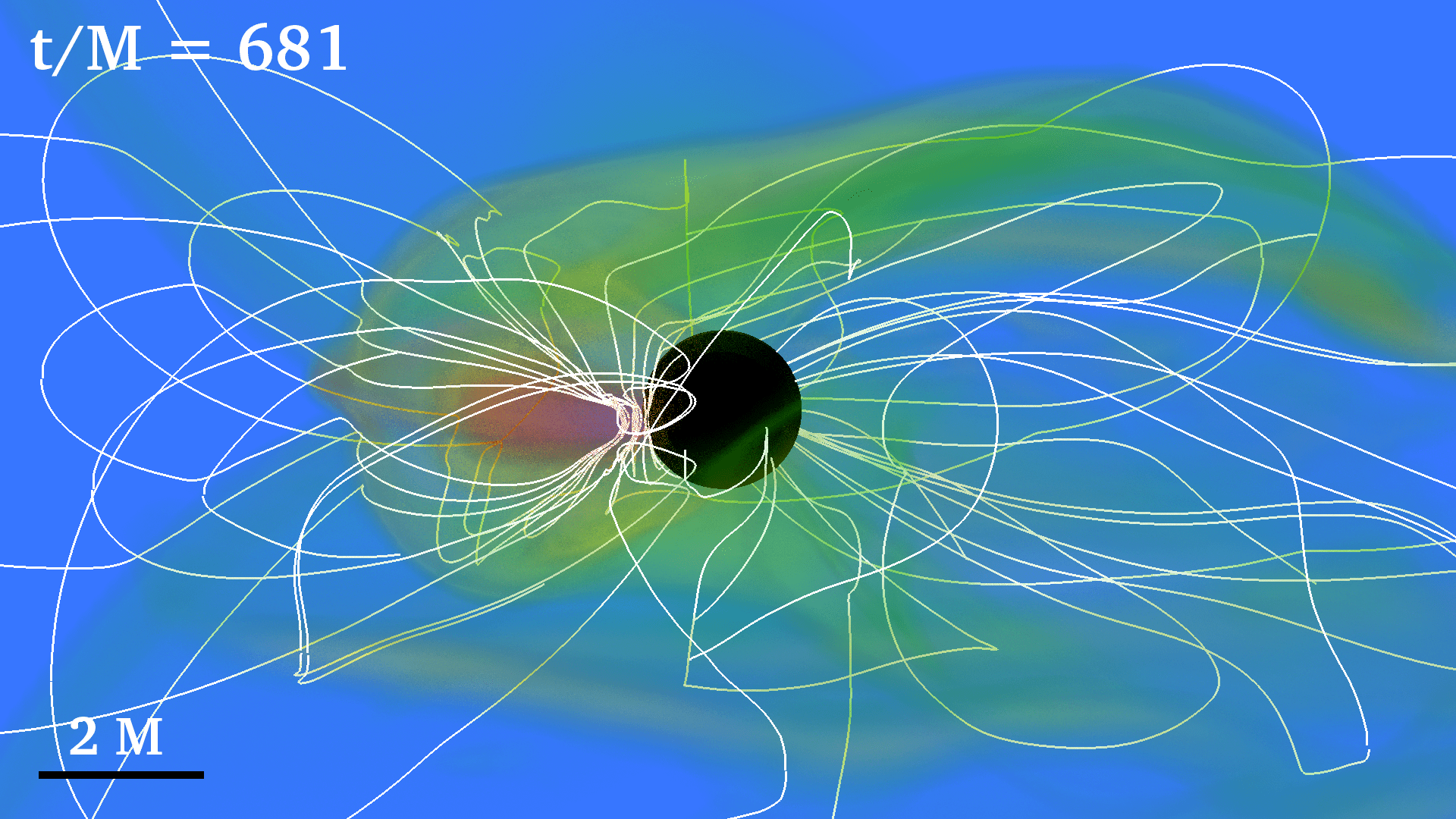
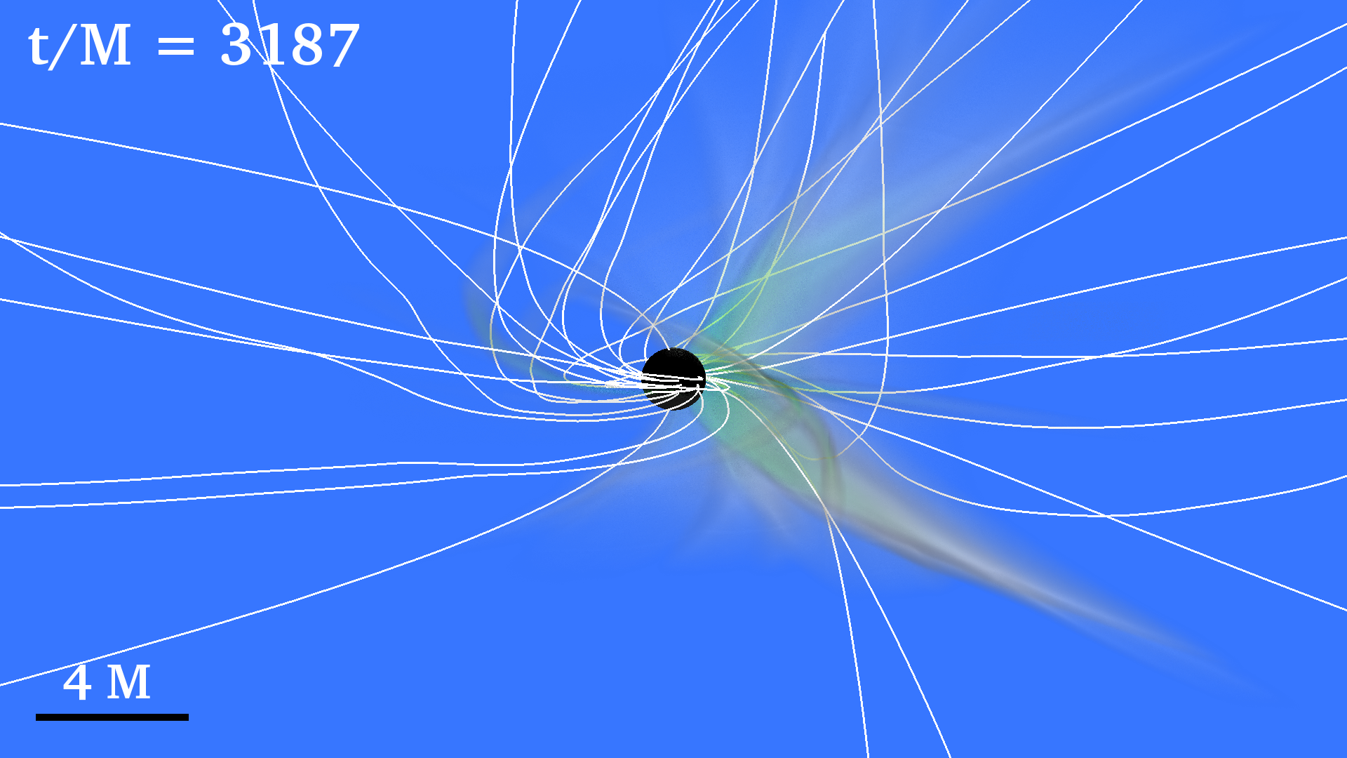
Figure 14: Volume rendering of rest-mass density $\rho_{0}$ normalized to its initial NS maximum value $\rho_{0}=8.92\times 10^{14}\,(1.4M_{\odot}/M_{\rm NS})^{2}\rm{g\,/cm}^{3}$ (log scale) at selected times for case Aliq5sp0.0 (see Table 1). White lines denote the magnetic field while the arrows denote the fluid velocity. The BH apparent horizon is denoted as a black sphere. Here $M=11.44(M_{\rm NS}/1.4M_{\odot})\rm km=3.81\times 10^{-2}(M_{\rm NS}/1.4M_{\odot})\rm ms$.

Fig 14 summarizes the evolution of this case starting from the insertion of the magnetic field (left panel), through the tidal disruption and merger (middle panel), and finally showing the outcome once the disk + BH remnant relaxes to a quasi–steady state (right panel). As expected, the star is somewhat disrupted before it plunges into the BH. Fig. 5 shows that during the first $t-t_{B}\sim 40M\sim 1.5(M_{\rm NS}/1.4M_{\odot})\rm ms$ following the onset of accretion the bulk of NS is quickly swallowed leaving an “orphan” BH remnant surrounded by a small, weakly magnetized cloud (less than $1\%$ of the rest-masss of the star) to form the accretion disk. By $t-t_{\rm GW}\approx 680M\sim 26(M_{\rm NS}/1.4M_{\odot})\rm ms$ the rest-mass accretion rate settles down to $\dot{M}=1.4\times 10^{-2}M_{\odot}/s$ and then decays slowly (see Fig. 6). Fig. 7 clearly shows that during that period there is basically no magnetic energy left (see Table 3) as the frozen-in magnetic field has been dragged into the BH during the plunge phase. We do not find evidence of magnetic field collimation or an outflow. Near to the end of the simulation the magnetic field strength above the BH poles is $\lesssim 10^{12.3}(1.4M_{\odot}/M_{\rm NS})$G.

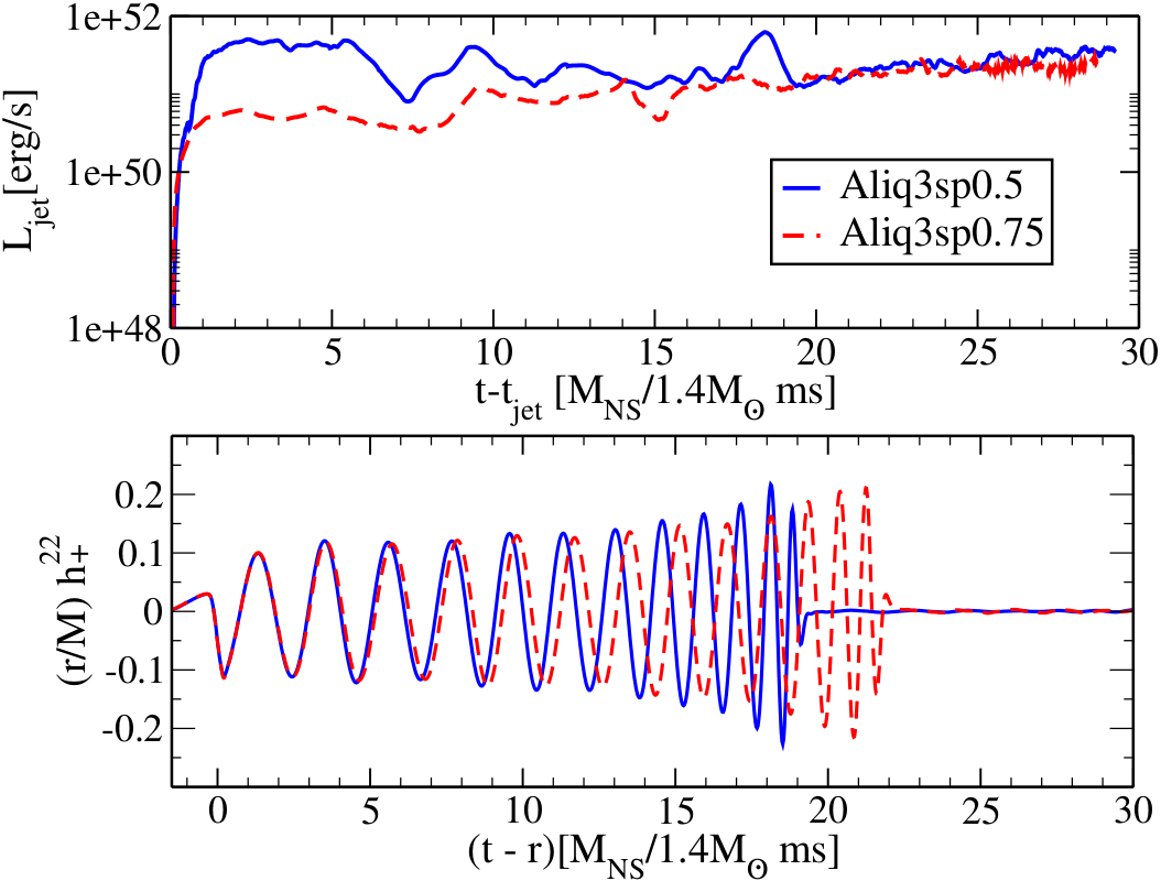
Figure 12: Outgoing EM (Poynting) luminosity for $t\geq t_{\rm jet}$ computed at a coordinate sphere of radius $r=100M\sim 760(M_{\rm NS}/1.4M_{\odot})\rm km$ (top panel), and (2,2) mode of the gravitational wave strain $h_{+}$ as functions of retarded time extracted at $r_{\rm ex}=80M\sim 606(M_{\rm NS}/1.4M_{\odot})\rm km$ (bottom panel) for case Aliq3sp0.5 (continuous line) and case Aliq3sp0.75 (dashed line).

Figure 13: Angular distribution of Poynting flux for case $\tilde{a}=0.5$, normalized by its peak value on a sphere of radius $60M=4600(M_{NS}/1.4M_{\odot})$km. Angles are defined with respect to a spherical coordinate system centered on the BH center, with the spin axis along the $z$ direction.

Notice that population synthesis studies have suggested that the most likely BHNS mass ratio may be $q=7:1$ Belczynski et al. (2008, 2010), although recently it has been suggested how low-mass BH formation channels may arise in BHNS Yang et al. (2018). For this high mass ratio configuration with a typical NS of compaction $\mathcal{C}=0.145$, the binary tidal separation is $R_{\rm tid}\sim 0.45M_{\rm BH}$. So, the critical spin at which tidal disruption occurs at the ISCO is $\tilde{a}=0.375$. As the basic ingredient for jet launching is a sizable magnetized disk, the above estimation suggests that high mass ratio BHNS configurations may be the progenitors of central engines that power sGRBs only if the spin of the BH companion is $\tilde{a}>0.4$ (see also Kyutoku et al. (2011); Foucart et al. (2018); Foucart (2012).

III.3 Effect of magnetic field orientation (case Tilq3sp0.75)

In the above section, we described the effects of the BH spin and mass ratio on the emergence of an incipient jet when the pulsar-like magnetic field seeded in the NS is aligned with the total orbital angular momentum of the system. In the following, we consider a BHNS configuration in which the BH companion has a spin of $\tilde{a}=0.75$, and the star is seeded with a pulsar-like magnetic field whose dipole magnetic moment is now tilted $90^{\circ}$ with respect to the orbital angular momentum (see left panel in Fig. 2).

The dynamics of the gas during tidal disruption, merger and early disk + BH phases are similar to those reported in Paper I, and summarized in Sec. III.1. This is not unexpected since the strength of the dynamical unimportant magnetic field in both cases is the same. However, by around $t-t_{\rm GW}=1600M\sim 40(M_{\rm NS}/1.4M_{\odot})$ms, by which time the accretion rate $\dot{M}$ settles down (see Fig. 6), the frozen-in magnetic field has been driven into a predominantly toroidal configuration in the disk, while in the atmosphere, in contrast to the spinning cases reported in Sec III.1 (see also Paper I), there is no a coherent poloidal magnetic field configuration (see right panel in Fig. 2). After evolving the remnant disk + BH for $t-t_{\rm GW}\gtrsim 4000M\sim 100(M_{\rm NS}/1.4M_{\odot})$ms, we do not find any evidence of magnetic field collimation or an outflow above the BH poles. As before, we compute the space-averaged value of the force-free parameter $b^{2}/(2\rho_{0})$ on a cubical region of a length side $2\,R_{\rm BH}$ just above the BH poles along the whole evolution (see Fig. 8). Following disruption, we observe that the plasma parameter peaks at two times its initial value and then slowly decreases until it falls to a value of $b^{2}/(2\,\rho_{0})_{|ave}~{}\sim 0.26$ (see Table 3). After about $t-t_{\rm GW}=5000M\sim 125M(M_{\rm NS}/1.4M_{\odot})\rm ms$ a persistent fall-back material toward the BH is observed.

When the magnetic field is aligned with the total angular momentum of the system, vertical field lines thread the BH prior to tidal disruption (see left top panel in Fig. 1 in Paper I). After disruption, these lines connect the polar regions of the BH to low-density debris in the atmosphere. Similarly, fluid elements in the disk are linked to other fluid elements in the disk, and to those ejected during the disruption, through external vertical magnetic lines (see right top panel in Fig. 1 in Paper I). These two effects induce a strong poloidal magnetic field in the BHNS remnant. By contrast, in the tilted case Tilq3sp0.75, horizontal field lines mainly thread the BH prior to tidal disruption (see left panel in Fig. 2). After disruption, these lines can only connect the BH poles to the inner part of the new–born disk, and they are rapidly wound to a predominantly toroidal configuration. Also, fluid elements in the disk are linked to other fluid elements in the disk, and to the low-density debris in the atmosphere, through external predominantly horizontal field lines. The BHNS remnant hence lacks a coherent poloidal magnetic field component (see right panel in Fig. 2).

While the properties of the disk + bh remnant, such as BH spin, mass, and accretion rate, are approximately independent of the magnetic field topology (see Table 3), the emergence of the jet seems to be very sensitive to it. As it was pointed out in Beckwith et al. (2008), a poloidal magnetic field component with a consistent sign in the vertical direction is required to launch and support a jet.

The above results indicate that there is a threshold value of the tilt angle of the dipole magnetic moment with respect to the orbital angular momentum below which the poloidal dipole magnetic field component is suppressed, and with it the emergence of a jet.

III.4 Universal model

Recently we proposed a “universal” analytic model in Shapiro (2017) that estimates a number of global parameters that characterize disk + BH remnants that launch jets following BHNS mergers, BHBH mergers immersed in magnetized disks, and the collapse of massive stars. The jets are powered by the BZ mechanism and the parameters are determined by only a couple of nondimensional ratios characterizing the remnant system. This model predicts the characteristic density in the accretion disk, the strength of the magnetic field above the BH poles, the rest-mass accretion rate after the system has reached a quasi-stationary state, and most significatively the EM (Poynting) luminosity as follows (see Eqs. 11-13 in Shapiro (2017)):

$$\rho\,M_{\rm BH}^{2}\sim\frac{1}{\pi}\,\left(\frac{M_{disk}}{M_{\rm BH}}\right)\,\left(\frac{M}{R_{disk}}\right)^{3}\,,$$ (14)

$$B_{p}^{2}\,M_{\rm BH}^{2}\sim 8\,\left(\frac{M_{disk}}{M_{\rm BH}}\right)\,\left(\frac{M}{R_{disk}}\right)^{3}\,,$$ (15)

$$\dot{M}_{\text{eq}}\sim 4\,\left(\frac{M_{disk}}{M_{\rm BH}}\right)\,\left(\frac{M}{R_{disk}}\right)^{3}\,[\dot{\mathcal{M}}_{0}]\,,$$ (16)

$$L_{BZ}\sim\frac{1}{10}\,\left(\frac{M_{disk}}{M_{\rm BH}}\right)\,\left(\frac{M_{\rm BH}}{R_{disk}}\right)^{3}\,\left(\frac{a}{M_{\rm BH}}\right)^{2}\,[\mathcal{L}_{0}]\,,$$ (17)

where $\mathcal{L}_{0}\equiv c^{5}/G=3.6\times 10^{59}\rm erg/s$ and $\dot{\mathcal{M}}_{0}\equiv c^{3}/G=2.0\times 10^{5}M_{\odot}/\rm s$. Table 4 shows a comparison of our simulations results with the model predictions, i.e. using as input the data in Table 3 to calculate the nondimensional ratios. We find that within an order of magnitude, the results are consistent. As was pointed out in Shapiro (2017), while there exist different formation scenarios for forming disk + BH systems, and their disk masses, densities and magnetic field strength vary by orders of magnitude, these features conspire to generate jet Poynting luminosities that all lie in the narrow range of $10^{52\pm 1}\rm erg/s$. Interestingly, these luminosity distributions mainly reside in the same narrow range characterizing the observed luminosity distributions of over 400 short and long GRBs Li et al. (2016).

IV Conclusions

The coincident detection of gravitational radiation (event GW170817) with short gamma ray bursts (GRB 170817A), detected $\sim 1.7\rm s$ after the inferred binary merger time Abbott et al. (2017b), confirm that merging compact binaries, containing at least one neutron star, can be the progenitors of the engine that powers sGRBs as proposed by Paczynski (1986); Eichler et al. (1989); Narayan et al. (1992). This single multimessenger detection has been already used to impose some constraints on the maximum mass of a spherical neutron star Margalit and Metzger (2017); Shibata et al. (2017); Ruiz et al. (2018); Rezzolla et al. (2018), on the tidal deformability, on the radius of the star Most et al. (2018); Abbott et al. (2017a, 2018); Radice et al. (2018); Bauswein et al. (2017), and other properties of the progenitor stars.

We recently reported the first self-consistent numerical calculations in full GR that demonstrate that the remnant of magnetized BHNS mergers can launch an incipient jet if the star is initially seeded with a dipole magnetic field that extends from the NS interior into a pulsar-like exterior magnetosphere Paschalidis et al. (2015). Here we survey different BHNS configurations that differ in the initial BH spin, mass ratio, and magnetic field topology to study the robustness of the jet launching scenario. Although the numerical studies reported here are illustrative and not exhaustive, they suggest the following:

Varying the initial spin of the BH companion in the binary from $\tilde{a}=-0.5$ to $0.5$, we observe that only the higher spin BHNS configuration launches a jet. In the antialigned case Aliq3sm0.5, the star basically plunges into the black hole leaving a weakly magnetized matter (less than $1\%$ of the initial rest-mass of the star) to form the disk (see Table 3). We do not find any evidence of large-scale magnetic field collimation or an outflow for this case. By contrast, in Aliq3sp0.0 we did observe magnetic field collimation above the BH poles, but after $t-t_{\rm GW}\sim 7000M\sim 175(M_{\rm NS}/1.4M_{\odot})$ms the magnetic pressure gradients were still too weak to launch an outflow. The lack of an outflow may be attributed to the persistent fall-back toward the BH observed as we terminated the simulation. When the atmosphere above the BH poles becomes thinner as the accretion proceeds, we anticipate that the magnetic pressure may eventually overcome the ram pressure. However, jet launching may not be possible if the onset time is longer than the lifetime of the accretion disk [$\tau_{\rm disk}\sim 0.36(M_{\rm NS}/1.4M_{\odot})$s]. The mass of the disk is determined by how far from the ISCO tidal disruption occurs. According, for a given NS companion, the above results indicate that there is a threshold value for the initial BH spin below which the jet launching cannot occur.

Varying the mass ratio of our BHNS configurations from $q=3:1$ to $q=5:1$, we find that only remnants with sizable accretion disks, and consequently considerable magnetic energy, may launch a jet. Taking into account population synthesis studies (see e.g. Belczynski et al. (2008, 2010)) that suggest that the most likely BHNS mass ratio may be $q=7:1$, we estimated that the critical spin at which tidal disruption occurs at the ISCO is $\tilde{a}=0.4$ (see also Kyutoku et al. (2011)). As the basic ingredient for jet launching is a sizable magnetized disk, the above estimate suggests that high mass ratio BHNS systems can be the central engines that power sGRBs only if the binary contains a highly spinning BH ($\tilde{a}\gtrsim 0.4$).

Finally, varying the direction of the magnetic field with respect to the total angular momentum of the system from an aligned configuration to a $90^{\circ}$-tilted configuration, we found that the disk + BH remnant in the latter case lacks of a coherent poloidal magnetic field configuration. At after about $t-t_{\rm GW}\sim 4000M\sim 100(M_{\rm NS}/1.4M_{\odot})\rm ms$ we did not see any indication of magnetic field collimation or an outflow. A poloidal magnetic field component with a consistent sign in the vertical direction is required to launch and support a jet Beckwith et al. (2008). These results suggest thus that there may also be a threshold value of the tilt angle of the magnetic dipole moment above which there are no jets.

A caveat is in order. Our GRMHD simulations do not account for all the physical processes involved in BHNS mergers. In particular, it has been suggested that neutrino annihilation in disk + BH systems may carry away a significant amount of energy from inner regions of the accretion disks that may be strong enough to power jets Popham et al. (1999); Di Matteo et al. (2002); Chen and Beloborodov (2007); Lei et al. (2013); Just et al. (2016). Recently, it was suggested in Lei et al. (2017) that the emergence of a jet in slowly BH + spinning disk systems may be triggered by neutrino-annihilation and then by the BZ mechanism, leading to a transition from a thermally-dominated fireball to a Poynting EM-dominated flow as is inferred for some GRBs, such as GRB 160625B Zhang et al. (2018). We plan to study such processes in the future.