Second release of the CoRe database of binary neutron star merger waveforms

Abstract

We present the second data release of gravitational waveforms from binary neutron star merger simulations performed by the Computational Relativity (CoRe) collaboration. The current database consists of 254 different binary neutron star configurations and a total of 590 individual numerical-relativity simulations using various grid resolutions. The released waveform data contain the strain and the Weyl curvature multipoles up to $\ell=m=4$. They span a significant portion of the mass, mass-ratio, spin and eccentricity parameter space and include targeted configurations to the events GW170817 and GW190425. CoRe simulations are performed with 18 different equations of state, seven of which are finite temperature models, and three of which account for non-hadronic degrees of freedom. About half of the released data are computed with high-order hydrodynamics schemes for tens of orbits to merger; the other half is computed with advanced microphysics. We showcase a standard waveform error analysis and discuss the accuracy of the database in terms of faithfulness. We present ready-to-use fitting formulas for equation of state-insensitive relations at merger (e.g. merger frequency), luminosity peak, and post-merger spectrum.

1 Introduction

The first observation of gravitational waves (GWs) from a binary neutron star (BNS) coalescence accompanied by electromagnetic (EM) signals marked a milestone in GW astronomy. Numerical relativity (NR) simulations are the main tool to explore the merger dynamics in the strong-field regime and aid the development of BNS gravitational waveforms that are necessary for GW detection and parameter estimation. The largest NR waveforms public catalogs contain data from thousands of binary black holes (BBHs) simulations, covering a significant portion of the mass-ratio and spin parameter space for quasi-circular mergers [1, 2, 3, 4, 5, 6, 7] and explore mergers from eccentric and generic orbits [4, 5, 6]. Public waveforms from simulations of binaries with NSs are more limited, and include the CoRe  database [8] (164 binaries at different resolutions for a total of 367), the SACRA-MPI [9, 10] (46, total 276), the SXS (2, total 6) [11, 3], among others [12, 13]. These waveforms are crucial for developing accurate inspiral-merger GW templates with tidal effects [14, 15, 16, 17, 18, 19, 20, 21, 22, 23, 24, 25, 26] and postmerger emission [27, 28, 29, 30, 31, 32, 33, 34, 35, 36, 37, 38] with direct applications to equation of state (EOS) constraints [39, 40, 41, 42]. The NR simulations performed for these waveforms are also key to determine the properties of the remnants from the binary parameters and the input physics (EOS, mass, spins, etc.), e.g. [43, 44, 45, 46, 47, 48, 49, 50, 51, 27] (see also [52, 53] for recent reviews). Consequently, new and extended data releases are necessary to support research in the field of GW astronomy.

Here, we present a new release of the CoRe database that comprises 90 new physically distinct BNS configurations at multiple resolutions, for a total of 254 binaries and 590 simulations. The new release includes GW strains and Weyl multipoles information up to the $(\ell,m)=(4,4)$ mode. The new data were computed in simulations presented in Refs. [54, 55, 56, 57, 58, 59, 60, 61, 62, 63, 64, 65, 66] and include BNS waveforms consistent with the GW events GW170817 [67, 56, 58, 59] and GW190425 [68, 66].

The paper is organized as follows. Sec. 2 summarizes the employed simulation techniques. Sec. 3 describes the physics content of the database and the impact of the binary parameters on the waveforms. Sec. 4 presents a full merger waveform error analysis for a case study, and gives an overview of the average accuracy of the data. Sec. 5 presents, as a first application of the database, ready-to-use EOS-insensitive fitting formulas for the GW frequency, amplitude and the peak luminosity that characterize the merger as well as analogous relations for the post-merger GW spectra.

The CoRe  database is hosted on the public gitlab server

https://core-gitlfs.tpi.uni-jena.de/core_database

Associated code repositories and resources can be accessed from

http://www.computational-relativity.org/

In particular, we provide the python package watpy to ease the checkout of the data and perform standard waveform analyses.

1.1 Notation

NR data are computed in geometrized units $c=G=1$ and solar masses ${\rm M_{\odot}}=1$; we use these units also in this paper unless explicitly indicated. We recall that $GM_{\odot}/c^{3}\simeq 4.925490947~{}\mu$s and $GM_{\odot}/c^{2}\simeq 1.476625038$ km. The binary mass is $M=m_{1}+m_{2}$, where $m_{1,2}$ are the gravitational masses of the two stars. The mass ratio is defined as $q=m_{1}/m_{2}\geq 1$, and the symmetric mass ratio is $\nu=m_{1}m_{2}/M^{2}\in[0,1/4]$, where $\nu=1/4$ corresponds to the equal-mass case, whereas $\nu\rightarrow 0$ for very unequal masses. The dimensionless, mass-rescaled spin vectors are denoted with ${\boldsymbol{\chi}}_{i}$ for $i=1,2$ and the spin components aligned with the orbital angular momentum L are labeled as $\chi_{i}={\boldsymbol{\chi}}_{i}\cdot\textbf{L}/|\textbf{L}|$. The effective spin parameter $\chi_{\rm eff}$ is defined as the mass-weighted aligned spin,

$$\chi_{\rm eff}=\frac{m_{1}\chi_{1}+m_{2}\chi_{2}}{M}\,.$$ (1)

Similarly, one can define the spin parameter [69],

$$\hat{S}=\left(\frac{m_{1}}{M}\right)^{2}\chi_{1}+\left(\frac{m_{2}}{M}\right)^{2}\chi_{2}.$$ (2)

The quadrupolar tidal polarizability parameters are defined as $\Lambda_{i}=({2}/{3})\,k_{2,i}\,C_{i}^{-5}$ for $i=1,2$ [70], where $k_{2,i}$ and $C_{i}$ are respectively the $\ell=2$ gravito-electric Love numbers and the compactness of the $i$-th neutron star (NS). The tidal coupling constant is [70] 

$$\kappa^{\rm T}_{2}=3\nu\,\left[\left(\frac{m_{1}}{M}\right)^{3}\Lambda_{1}+(1\leftrightarrow 2)\right]\,,$$ (3)

that, similarly to the reduced tidal parameter [71]

$$\tilde{\Lambda}=\frac{16}{13}\frac{(m_{1}+12m_{2})m_{1}^{4}\Lambda_{1}}{M^{5}}+(1\leftrightarrow 2)\,,$$ (4)

parametrizes the leading-order tidal contribution to the binary interaction potential and waveform phase (note that $\kappa^{\rm T}_{2}=\frac{3}{16}\tilde{\Lambda}$ for $q=1$.)

The radiated GW (polarizations $h_{+}$ and $h_{\times}$) is decomposed in $(\ell,m)$ multipoles as

$$h_{+}-{\rm i}h_{\times}=D_{L}^{-1}\sum_{\ell=2}^{\infty}\sum_{m=-\ell}^{\ell}h_{\ell m}(t)\,{}_{-2}Y_{\ell m}(\iota,\varphi),$$ (5)

where $D_{L}$ is the luminosity distance, ${}_{-2}Y_{\ell m}$ are the $s=-2$ spin-weighted spherical harmonics and $\iota,\varphi$ are respectively the polar and azimuthal angles that define the orientation of the binary with respect to the observer. Each mode $h_{\ell m}(t)$ can be decomposed in amplitude $A_{\ell m}(t)$ and phase $\phi_{\ell m}(t)$ as

$$h_{\ell m}(t)=A_{\ell m}(t)\,{\rm e}^{-{\rm i}\phi_{\ell m}(t)}\,,$$ (6)

with a related GW frequency

$$\omega_{\ell m}(t)=\frac{{\rm d}}{{\rm d}t}{\phi_{\ell m}}(t)\,.$$ (7)

A dimensionless frequency $\hat{\omega}=GM\omega$ relates to the frequency in Hz according to the formula

$$f=\frac{\omega}{2\pi}\simeq 32.3125\,\hat{\omega}\,\left(\frac{M_{\odot}}{M}\right)\,\mbox{kHz}\,.$$

The GW strain modes are related to the Weyl $\Psi_{4}$ curvature modes $\psi_{\ell m}$ by

$$\ddot{h}_{\ell m}=\psi_{\ell m}\,.$$ (8)

CoRe simulations compute only $\psi_{\ell m}$ at different extraction radii $R$. However, the above equation can be integrated to obtain the strain, either by using the fix-frequency integration method [72] or directly in the time-domain and performing a polynomial correction, e.g. [73, 74, 14]. Comparisons between analytical and NR data often use the Regge-Wheeler-Zerilli normalized multipolar waveforms $\Psi_{\ell m}$,

$$h_{\ell m}=\sqrt{(\ell+2)(\ell+1)\ell(\ell-1)}\,\Psi_{\ell m}\,$$ (9)

The radiated energy is obtained as [46]

$$\mathcal{E}_{\rm{rad}}=\frac{1}{16\pi}\sum_{\ell=2}^{\ell_{\rm{max}}}\sum_{m=-\ell}^{\ell}\int_{0}^{t}{\rm d}t^{\prime}|D_{L}\dot{h}_{\ell m}(t^{\prime})|^{2}\,,$$ (10)

whereas the angular momentum is computed as

$$\mathcal{J}_{\rm{rad}}=\frac{1}{16\pi}\sum_{\ell=2}^{\ell_{\rm{max}}}\sum_{m=-\ell}^{\ell}\int_{0}^{t}{\rm d}t^{\prime}m\left[D_{L}^{2}h_{\ell m}(t^{\prime})\dot{h}^{*}_{\ell m}(t^{\prime})\right]\,.$$ (11)

The data released are computed with $\ell_{\rm{max}}=4$. The binary dynamics can be characterized by the binding energy and the orbital angular momentum, we therefore work with the binding energy per reduced mass, obtained by substracting the GW energy loss from the initial ADM mass, $E_{b}=[(M_{\rm{ADM}}(t=0)-\mathcal{E}_{\rm{rad}})/M-1]\nu^{-1}$ and the dimensionless rescaled angular momentum $j=(\mathcal{J}_{\rm{ADM}}(t=0)-\mathcal{J}_{\rm{rad}})(M^{2}\nu)^{-1}$, see [75, 46] for details. The GW luminosity peak is computed as

$$L_{\rm{peak}}=\max_{t}\frac{{\rm d}\mathcal{E}_{\rm{rad}}(t)}{{\rm d}t}\approx\max_{t}\left[\frac{1}{16\pi}\sum_{\ell=2}^{\ell_{\rm{max}}}\sum_{m=-\ell}^{\ell}\left|D_{L}\dot{h}_{\ell m}(t)\right|^{2}\right].$$ (12)

The moment of merger is defined as the time of the peak of $A_{22}(t)$, and referred simply as “merger” when it cannot be confused with the coalescence/merger process. Waveforms are often shown in terms of the retarded time

$$u=t-r_{*}(r)=t-\left[r+r_{S}\ln\left(\frac{r}{r_{S}}-1\right)\right]\,,$$ (13)

where $r$ is the coordinate extraction radius in the simulations (assumed close to the isotropic Schwarzschild radius), $r_{*}$ is the associated tortoise Schwarzschild coordinate, and $r_{S}=2M$ is the Schwarzschild radius.

2 Methods

2.1 Initial data

Initial data for CoRe simulations are generated solving Einstein’s constraint equations in the conformal thin sandwich (CTS) formalism [76] assuming a helical Killing vector and imposing hydrodynamical equilibrium for the NS’s fluid [77, 78]. It is assumed that the fluid is either irrotational or in a quasi-equilibrium state with constant rotational velocity, which allows for consistent simulations of NS with spin [79, 80]. In the latter formalism, the rotational part $w^{a}$ of the fluid’s velocity is determined by an angular velocity parameter $\omega^{i}$ as

$$w_{i}=\epsilon_{ijk}\omega^{j}(x^{k}-x^{k}_{*})\,,$$ (14)

where $x^{k}_{*}$ are the coordinates of the NS center. Possible definitions of spin for a star in a binary are discussed in Refs. [46, 81, 82]. The spin parameters given in the CoRe database are defined to be those of single NSs in isolation with the same rest mass and the same $\omega^{i}$ as the BNS components [46, 81, 83]. To construct initial data with abritrary eccentricities, we use an extension of the helical symmetry condition that is based on approximate instantaneous first integrals of the Euler equations and a self-consistent iteration of the CTS equations [84]. This method also allows us to create low-eccentricity initial data in quasi-circular orbits using an iterative procedure that combines initial data and evolution codes [81] (see also [85, 86, 87]).

CoRe initial data are calculated using either Lorene [88, 89, 90] or SGRID [91, 92, 79, 80, 81, 83]. Both codes use multi-domain pseudospectral methods to solve the CTS equations and surface-fitting coordinates that minimize spurious stellar oscillations at the beginning of the evolutions and guarantee accurate determination of the initial binary global quantities. Lorene can construct irrotational binaries with either piecewise polytropic or tabulated EOS. In the latter case, they are often obtained as cold, $\beta$-equilibrated slices of finite-temperature, composition dependent EOS. SGRID can generate irrotational or spinning binaries with piecewise polytropic EOS and arbitrary (or reduced) eccentricity. In particular, SGRID can simulate BNS in which the individual stars rotate close to the breakup spin and have masses which are $\sim 98\%$ of the maximum supported NS mass allowed by the EOS [83]. Evolutions of initial data generated with SGRID and Lorene were compared in Ref. [46], where we found them to be in good agreement.

Initial data in quasi-circular orbits are characterized by the following global quantities of the 3+1 hypersurfaces: the total baryon mass $M_{b}$ (a conserved quantity along the evolution); the total binary gravitational mass $M$, i.e., the sum of the two gravitational masses of the bodies in isolation; the initial orbital frequency $\Omega\simeq\omega_{22}/2$ and the corresponding ADM mass $M_{\rm ADM}$ and angular momentum $J_{\rm ADM}$.

2.2 Evolution codes

CoRe simulations evolve initial data using a free-evolution approach to 3+1 Einstein field equations based on the hyperbolic conformal formulations BSSNOK [93, 94, 95] or Z4c [96, 97, 98]. The latter is used for all of the newly released data (Ref. [65] also uses BSSNOK). The (1+log)-lapse and gamma-driver shift conditions are used for the gauge sector. The general relativistic hydrodynamics is solved in first-order conservative form [99]. Wave extraction is typically performed on coordinate spheres at finite radius placed in the wave zone of the computational domain (typically $R\sim 500-1000~{}{\rm M_{\odot}}$) and calculating the Weyl pseudoscalar $\Psi_{4}$, see e.g. [100] for details.

Simulations are performed with two independent mesh-based codes: BAM [100, 101] and THC [102, 103, 104], both developed and maintained within our collaboration. These codes employ adaptive mesh refinement (AMR) techniques in which the domain consists of a hierarchy of nested Cartesian grids (refinement levels). The grid spacing of each refinement level in each direction is half the grid spacing of its surrounding coarser refinement level. Finite difference stencils are used for the spatial discretization of the metric variables (usually at fourth order accuracy), and high resolution shock-capturing methods for the hydrodynamics. The Berger-Oliger or Berger-Colella algorithm is employed during the explicit mesh evolution. The latter is performed with the method of lines and Runge-Kutta schemes of third or fourth order accuracy in time. The innermost levels move dynamically during the time evolution following the motion of the NS such that the strong field region around a NS is always covered with the highest resolution. Both codes employ a hybrid OpenMP/MPI parallelization strategy and show good parallel scaling up to thousands of cores.

BAM implements high-order finite-differencing WENO schemes [19] and, more recently, an entropy-flux-limited (EFL) scheme [65], that is better adapted to the treatment of the NS surface, to accurately simulate multiple orbits and GWs from inspiral-mergers. The typical grid configurations for these simulations consist of seven refinement levels, where the innermost level split into two boxes covering each of the NSs. Standard grid parameters for resolution studies are chosen with $n_{m}\in[96,256]$ points per direction in each inner (moving) level and $n\in[144,512]$ for the outer levels. The minimal grid spacing in each direction is $\Delta\sim[0.059,0.321]~{}{\rm M_{\odot}}$ and the maximal resolution reached in the released simulation is $\Delta\sim 0.059~{}{\rm M_{\odot}}$. Symmetries can be imposed to reduce the computational cost of certain problems. For example, aligned-spin BNS are often simulated in bitant symmetry ($z>0$ volume). The simulation parameters can vary for each simulation; the relevant ones are reported in the CoRe metadata.

THC implements both high-order finite-differencing schemes [105] and Kurganov-Tadmor-type central schemes. The latter are preferentially used with simulations with microphysics. THC can make use of microphysical EOS, and implements various neutrino transport schemes [106, 54, 107] (see below) and subgrid-scale treatment of turbulent mixing and dissipation (GRLES) [108, 61] to accurately simulate remnants and postmerger dynamics. Most of the GRLES data in the current release employ an effective model for turbulence based on the high-resolution magnetohydrodynamics simulation of Ref. [109], where the viscosity parameter is set to $\nu_{T}=\ell_{\rm mix}c_{s}^{2}$ and $c_{s}$ is the sound speed of the fluid. $\ell_{\rm mix}$ is typically defined to be a function of the rest-mass density calibrated with the general-relativistic magneto-hydrodynamics simulations of [109] (see [61]). THC builds on the Cactus framework [110] and the Einstein Toolkit [111, 112]. THC simulations use the Carpet adaptive mesh refinement driver for Cactus[113], which implements both vertex centered and cell-centered adaptive mesh refinement with flux correction [114, 115]. The grid structure used in the THC simulations is similar to that used in BAM. The grid structure is specified by the resolution at the coarsest refinement level and at the location of the center of the neutron stars. The refinement levels on the grid hierarchy do not have to be connected and Carpet can merge different regions to create grids with complex topology. The standard resolution setup of the THC simulations uses a resolution of $\Delta=0.125\ M_{\odot}$ in every direction on the finest refinement level. The maximal resolution reached in the released simulation is $\Delta\simeq 0.08\ M_{\odot}$. The typical CFL is $0.125$. However, an even lower CFL of $0.0625$ is used on the coarsest grid to handle the gamma-driver source term in the shift evolution equation. All THC simulations included in the current release of the CoRe database use bitant symmetry.

2.3 EOS models

CoRe simulations currently employ 18 different EOS models for the neutron star matter. BAM data are computed using analytical EOS in the form

$$P(\rho,\epsilon)=P_{\rm pwp}(\rho)+(\gamma_{\rm th}-1)\rho(\epsilon-\epsilon_{\rm pwp})\,,$$ (15)

where $P_{\rm pwp}(\rho)$ is a given piecewise politropic EOS model [116]. It prescribes also a value $\epsilon_{\rm pwp}$ for the specific internal energy given the rest mass density $\rho$, augmented with a $\gamma$-law “thermal” pressure term (usually, $\gamma_{\rm th}=1.75$ [45, 117]). The specific parameters we employ for the piecewise polytropic EOS mimic well-established zero-temperature EOS models [116]; tables of these parameters are available on the CoRe website .

The current release significantly extends the data computed with finite-temperature EOS over the first release. The release includes data from seven finite-temperature EOS, used in the calculation of Refs. [54, 55, 56, 57, 58, 66, 59, 63]. The finite-temperature EOS include the following models: BHB$\Lambda\phi$ [118], BLh [119, 120], BLQ [120, 63], DD2 [121, 122], LS220 [123], SFHo [124], SLy4/SRO [125, 126].

All these EOS include neutrons, protons, nuclei, electrons, positrons, and photons as relevant thermodynamics degrees of freedom. The ALF2 [127] and BLQ EOS [120, 63] are hybrid models accounting for deconfined quark matter. BHB$\Lambda\phi$ is a hadronic model that includes $\Lambda$ hyperons [118, 128].

Cold, neutrino-less $\beta$-equilibrated matter described by these microphysical EOS predicts NS maximum masses and radii within a larger range than that allowed by current astrophysical constraints, including GW170817 [129, 40, 41]. Figure 1 shows the mass-radius diagram and the quadrupolar tidal polarizability parameter-mass diagram of these EOS. The largest radius of a $M=1.4~{}{\rm M_{\odot}}$ NS is ${R_{1.4}^{\rm TOV}}\sim 15.21$ km (EOS 2H) and the smallest radius ${\sim}9.75$ km (EOB 2B). The smallest maximum mass is ${M_{\rm max}^{\rm TOV}}\sim 1.70~{}{\rm M_{\odot}}$ (EOS H3), whereas the largest is ${M_{\rm max}^{\rm TOV}}\sim 2.83~{}{\rm M_{\odot}}$ (EOS 2H).

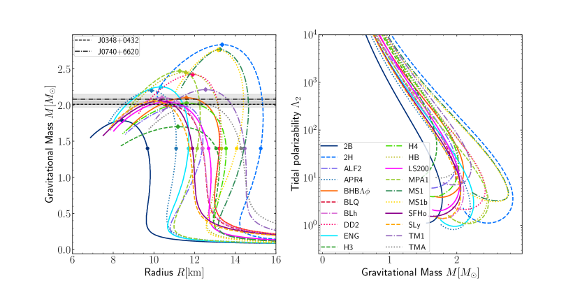
Figure 1: Mass-radius (left) and tidal polarizability-compactness (right) sequences of the available EOS. Diamond-shaped markers correspond to the maximum mass for each EOS, whereas the circle-shaped ones show the radius $R_{1.4}$ for a 1.4 ${\rm M_{\odot}}$ star. The black lines on the left panel show the current mass estimates of PSR J0348+0432 [130] and PSR J0740+6620 [131, 132] with their corresponding constraints (gray bands).

Most of these EOS can be found on the CoRe website in tabulated form. In the simulations, the EOS is called during the hydrodynamics evolution in order to compute the pressure from the rest-mass density, the temperature, and the electron fraction, i.e., in the form $p=P(\rho,T,Y_{e})$. Any relevant thermodynamical quantity is evaluated by multi-linear interpolating the tabulated values in $\log\rho$, $\log T$, and $Y_{e}$. As common in relativistic hydrodynamics, the EOS is called during the transformation from conservative to primitive variables. The latter takes place at each timestep and grid point and it involves a numerical root finding of the function $f(p):=p-P(\rho,\epsilon,Y_{e})$, where the specific internal energy $\epsilon$ is implicitly given by the temperature $T$ [133]. Hence, each root-finding step includes another root finder for the function $g(T)=\epsilon-{\cal E}(T)$ (see [134] for a discussion on computational efficiency and a non-standard approach based on neural networks.)

2.4 Microphysics

Most of the THC simulations account for the loss of energy and lepton number due to the net emission of neutrinos using a leakage scheme [133, 106]. Accordingly, effective neutrino leakage rates are computed as a physically motivated interpolation from the emission and diffusion rates. The latter require the knowledge of the optical depth of each computational zone in such a way as to recover the correct cooling time scale. Neutrino reabsorption is included in some simulations using the M0 scheme [106]. This scheme splits neutrinos in an optically thick component, treated with the leakage scheme, and a free-streaming component. The free-streaming neutrinos and their average energies are obtained by solving the radiative transfer equations on a set of radial rays (the so-called ray-by-ray approach) fully-implicitly in time. More recently, we have implemented an energy-integrated M1 scheme in THC [107]. The new scheme can self-consistently capture the diffusion of neutrinos from the merger remnant and its reabsorption in the ejecta. M1 simulations are not included in the current release of the database, but will be made public as soon as the associated publications have been accepted. Table 1 summarizes all neutrino reactions currently included in THC together with the reference in which the form of the rates we use are derived.

Table 1: Weak reaction rates and references for their implementation. We use the following notation $\nu\in\{\nu_{e},\bar{\nu}_{e},\nu_{x}\}$ denotes a neutrino, $\nu_{x}$ denote any heavy-lepton neutrino, $N\in\{n,p\}$ denotes a nucleon, and $A$ denotes a nucleus.

Reaction	Reference
$\nu_{e}+n\leftrightarrow p+e^{-}$	[135]
$\bar{\nu}_{e}+p\leftrightarrow n+e^{+}$	[135]
$e^{+}+e^{-}\rightarrow\nu+\bar{\nu}$	[136]
$\gamma+\gamma\rightarrow\nu+\bar{\nu}$	[136]
$N+N\rightarrow\nu+\bar{\nu}+N+N$	[137]
$\nu+N\rightarrow\nu+N$	[136]
$\nu+A\rightarrow\nu+A$	[138]

3 Overview

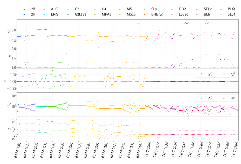
Figure 2: Summary of the CoRe database. The complete data are shown based on: the binary mass $M$, the mass ratio $q$, the individual dimensionless spins $\chi^{\rm{A,B}}_{z}$, the individual quadrupolar tidal parameters $\Lambda^{\rm{A,B}}_{2}$, the EOS and the employed resolution $\Delta$.

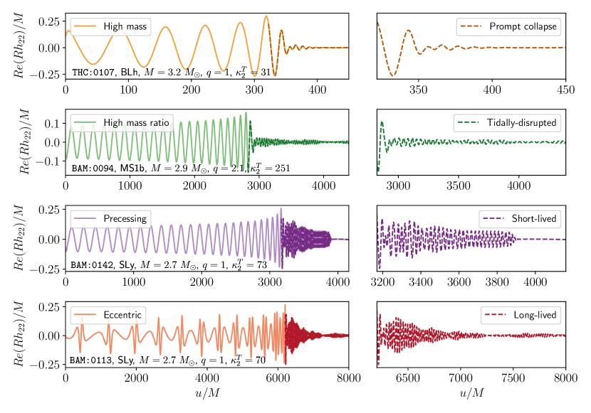
Figure 3: Representative waveforms from the CoRe database with their respective post-merger signals exemplifying the different morphologies influenced by the input physics (total mass of the binary, mass ratio, spins, and eccentricity).

CoRe simulations are performed for various binary masses, mass ratios, NS spins and EOS as summarized by Figure 2. They cover a significant portion of the BNS parameter space and allow to quantitatively explore the connection between the gravitational-wave morphology and the binary parameters in some detail. Figure 3 illustrates the variety of waveforms contained in the database. In the following, we give an overview of the database content and outline the connections between physics and waveform morphology.

The database contains waveforms from binaries with total masses ranging from $2.4~{}{\rm M_{\odot}}$ to around ${\sim}3.4~{}{\rm M_{\odot}}$ with 45 datasets reaching mass ratios larger than $q\gtrsim 1.4$ and up to $q=2.1$ [47, 58, 64]. EOS effect can be summarized to some extent  by the quadrupolar tidal polarizability parameters $\Lambda_{1,2}$ [70], where larger (smaller) values of $\Lambda_{i}$ are associated to stiffer (softer) EOSs. The most compact NSs (and most massive binaries) are associated with the smallest values of $\Lambda_{1,2}$ (and $\tilde{\Lambda}$), see the right panel of Fig. 1. The CoRe data encompasses well the mass and EOS variation for realistic BNSs. Waveforms from both irrotational and spinning (using the formalism outlined in Sec. 2.1) quasi-circular mergers are included [46, 48, 60]. For aligned spins, the individual dimensionless components range in $\chi_{z}\in[-0.25,0.5)$; about 7 datasets are from simulations with precession effects [48, 60]. The distribution of key parameters among the CoRe simulations is shown in Fig. 4.

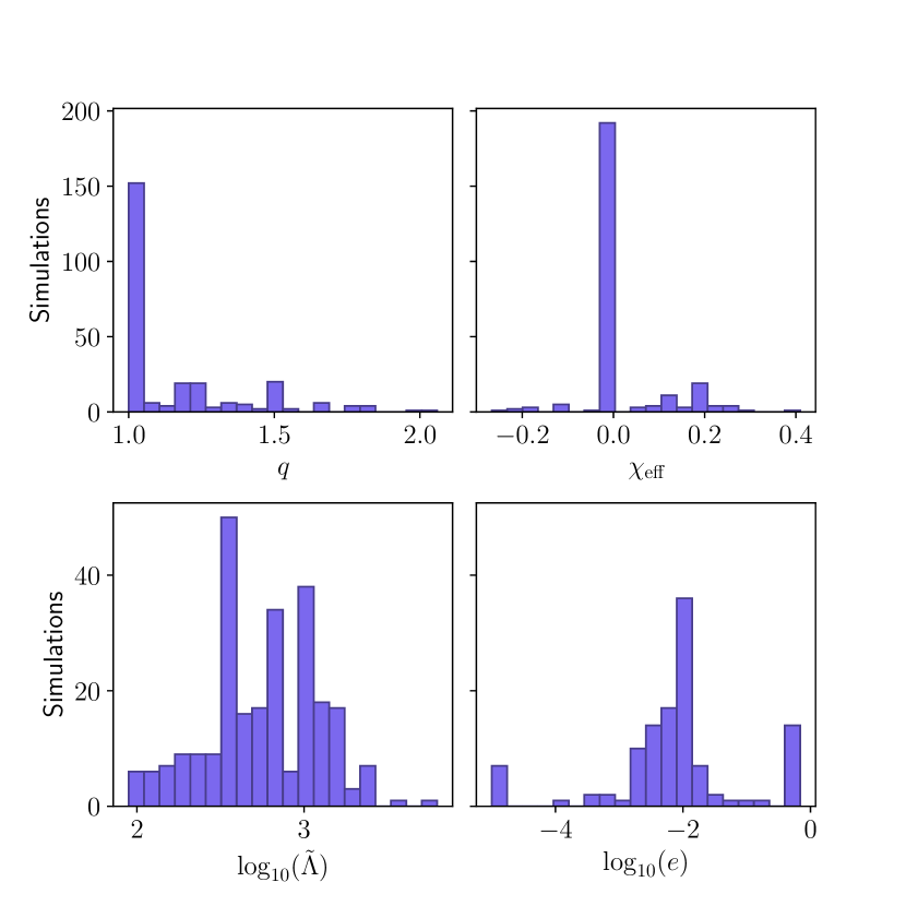
Figure 4: Distribution of the mass ratio $q$, and the effective spin parameter $\chi_{\rm eff}$, reduced tidal parameters $\tilde{\Lambda}$, and initial eccentricity of the 254 CoRe database configurations. Note that for some short simulations no reliable measure of eccentricity was possible.

Most of the CoRe waveforms are produced from quasi-circular mergers. The residual eccentricities of non-iterated quasi-circular initial data is usually $e\sim 10^{-2}-10^{-1}$, see the bottom right panel of Fig. 4. About 13 datasets have an initial eccentricity $e\lesssim 10^{-3}$ that was reduced through an iterative procedure employing the formalism described in Sec. 2.1. A subset of waveforms refer instead to eccentric mergers with initial eccentricity values as high as ${\sim}0.7$ [139, 106, 140]. In particular, the simulation in the bottom panels of Fig. 3 has an initial eccentricity of $0.55$.

The effects of mass-ratio, spin, and tides on the orbital dynamics can be studied by means of gauge-invariant energy curves $E_{b}(j)$, that are also publicly released. We illustrate this in Fig. 5 for a few examples. In the inspiral, the binary’s angular momentum $j$ decreases due to GW emission and the system becomes more bound ($E_{b}$ stays negative and $|E_{b}|$ increases). Equal mass ($\nu=1/4$) non-spinning BBH systems merge with $E_{b}\simeq-0.12$, indicating that about 3% of the binary mass was radiated in GWs to the moment of merger (marker in the figure). Tidal effects in BNS make the potential governing the relative dynamics more attractive. The tidal constribution to the potential at leading order is $\sim-\kappa^{\rm T}_{2}/r^{6}$, i.e. it is stronger for larger tidal polarizabilities $\Lambda_{1,2}$ and it is short-ranged thus affecting the motion mostly at high frequencies (small separations, $r$) towards merger. Consequently, the inspiral of an equal mass non-spinning BNS is faster than a binary black hole inspiral. The binding energy at the moment of merger is $|E_{b}|\sim 0.064$, which is smaller than the black hole case because the BNS system is less compact. Mass-ratio effects make the potential more repulsive, but are less effective than tides at high frequencies. The $q=2$ BNS shown in Fig. 5 merges at smaller values $|E_{b}|\sim 0.055$ than the equal mass because of tidal disruption. The remnant has also larger angular momentum $j\sim 3.6$ [59].

Spin-effects are dominated by the leading-order spin-orbit interaction; their character is thus repulsive or attractive depending on the projection of the spin on the orbital angular momentum [141]. This is analogous to what happens to corotating/counter-rotating circular orbits in Kerr spacetimes that move outwards (inwards) for antialigned (aligned) spin configurations with respect to the nonspinning case. In binary black hole simulations this effect has been named as “hang-up” effect [142]. In Fig. 5, the spinning BNS with $\hat{S}=0.1$ is more bound than the non-spinning BNS at the moment of merger with $E_{b}\sim-0.068$. Note that $j$ in this case includes the spin contribution. Moreover, the eccentric equal-mass case, contrary to the previous ones, shows brief moments of constant $E_{b}$ indicating the times when the NSs are apart (see inset of Fig. 5). Energy curves for BNS have been studied in detail in [46, 48, 60] to which we refer for more details. We stress that the properties of BNS systems at the moment of merger can be captured by EOS-insensitive (quasi-universal) relations [16]. The latter can be helpful in waveform modelling and used to estimate the properties of the remnant. We refer to Sec. 5 for further discussion.

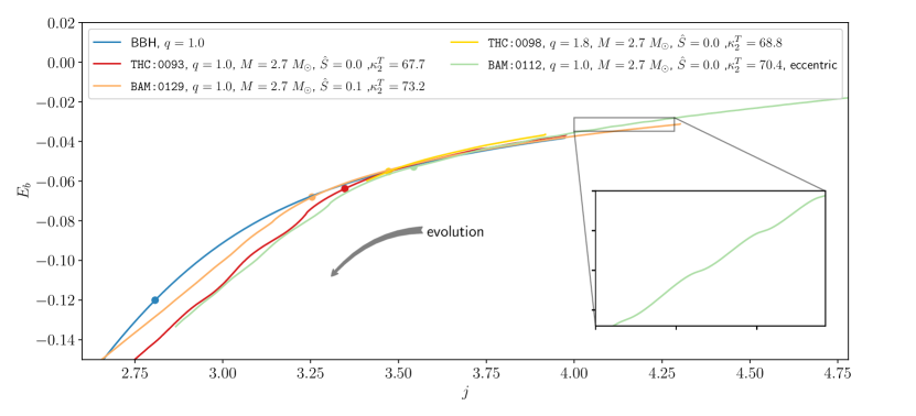
Figure 5: Energy curves $E_{b}(j)$ for selected binaries. The binary’s binding energy and angular momentum evolve in time from right to left along the cuves $E_{b}(j)$. The moment of mergers are indicated with a marker. The close up of BAM:0112 shows a modulation present due to its eccentric inspiral (see text).

High-mass BNS produce a remnant that promptly collapses to a black hole shortly after the moment of merger and before the two cores can bounce [52, 53]. Prompt collapse implies negligible shocked dynamical ejecta, because the bulk of the mass ejection comes from the first core bounce after their collision [54]. Prompt collapse can be characterized by a threshold mass $m_{\rm thr}=k_{\rm thr}{M_{\rm max}^{\rm TOV}}$, that mainly depends on the maximum mass of cold equilibria ${M_{\rm max}^{\rm TOV}}$ supported by the EOS [45, 143]. The recent analysis of Ref. [144], based on 227 finite-temperature EOS and CoRe data , found that the prompt collapse mass threshold for equal-mass non-spinning BNS is well described by an EOS-insensitive threshold

$$k_{\rm thr}=a\,{C_{\rm max}^{\rm TOV}}+b\,,$$ (16)

where ${C_{\rm max}^{\rm TOV}}$ is the compactness of the maximum NS mass, and $a=-3.36\pm 0.20$, $b=2.35\pm 0.06$. A prompt collapse waveform has a rapidly damped black hole ringdown after the moment of merger as shown in the top panels of Figure 3. Consequently, the postmerger GW signal is practically negligible for the sensitivities of both current and next-generation detectors. The lack of shocked ejecta and of a massive disc also implies that equal-mass prompt-collapse mergers have dim EM emission. However, for very asymmetric BNS with $q\gtrsim 1.4$, it is the tidal disruption of the secondary NS and its accretion onto the primary to trigger the gravitational collapse [58]. Thus, asymmetric mergers can be electromagnetically bright because they produce massive tidal dynamical ejecta and remnants with accretion discs of mass ${\sim}0.1~{}{\rm M_{\odot}}$. This prompt collapse process is mainly controlled by the incompressibility parameter of nuclear matter around the TOV maximum density [145]. A robust, EOS-insensitive criterion is not known in these conditions [58, 146, 147, 145, 148], but tidal disruption effects are subdominant to the mass effect; they produce maximal variations from the equal-mass criterion of ${\sim}8\%$ [144, 145].

Without prompt collapse, the evolution of a NS remnant is driven by the GWs emission of ${\sim}10^{53}~{}{\rm erg}$ lasting ${\lesssim}20$ milliseconds (GW-driven phase) [149, 150]. During this phase, a remnant that collapses to a black hole is called short-lived, while a remnant that settles to an approximately axisymmetric rotating NS is called long-lived. Examples of postmerger signals from these remnants are shown in the last two panels on the right of Figure 3, for the equal-mass case. The GW-driven phase is associated to a luminous GW transient that peaks at frequencies ${\sim}2-4\,$kHz [151, 152, 153, 27, 154, 28]. The spectrum of this transient is rather complex but has robust and well-studied features at a few characteristic frequencies. Most of the GW power is emitted in the $(2,2)$ mode at a nearly constant frequency $\omega_{22}(t)\approx 2\pi f_{2}$; the more compact and close to collapse the remnant is, the higher and more varying the $\omega_{22}(t)$ emission frequency is. The postmerger dynamics is primarily controlled by the masses of the two stars and the bulk properties of the zero-temperature EOS, in particular maximum TOV mass and compactness [52, 155]. Finite temperature and neutrinos do not produce qualitative differences, other than possibly on the time of gravitational collapse of the remnant [156]. Quantitative differences in the GW signal introduced by finite-temperature and neutrino effects are typically subdominant compared to finite-resolution uncertainties [157, 107]. On the other hand, microphysics plays a crucial role in the EM counterparts and nucleosynthesis from mergers, e.g., [158, 159, 106, 160, 161].

The remnant’s signal from asymmetric binaries with mass ratio $q\gtrsim 1.4$ carries the imprint of the tidal disruption during merger [47, 162, 58]. An example of such a waveform is shown in the second panels (top to bottom) of Figure 3. Comparing to the equal-mass long-lived case, the postmerger amplitude is significantly smaller because the asymmetric remnant does not experience the violent bounces of the symmetric remnant. For the same reason, the early-times modulations in frequency and amplitude present in the equal-mass case are significantly suppressed in the asymmetric case.

The evolution of a NS remnant beyond the GW-driven phase is uncertain at present. Explorations of the viscous phase using NR simulations have started [163, 59, 164], but they are still incomplete in many ways. While GW emission is expected to be significantly weaker than during merger, remnant’s instabilities might enhance GW emission. Current NR results suggest that BNS remnants have an excess of both gravitational mass and angular momentum after the GW-driven phase and when compared to equilibrium configuration with the corresponding baryon mass [165, 166]. Possible mechanisms to shed (part of) this energy are CFS [167, 168] and one-arm instabilities [169, 170, 171] that would lead to potentially detectable, long GW transients at ${\lesssim}1\,$kHz. Example of such waveforms are THC:0028, THC:0029, and THC:0036 [170].

Finally, CoRe data are available for multiple grid resolutions as discussed in Sec. 2 and shown by Fig. 2. Most of the newly released data contain high resolution simulations with a minimum grid spacing as low as $\Delta\sim 0.06~{}{\rm M_{\odot}}$, e.g., the NS are resolved with a uniform mesh of spacing ${\sim}88.4$ meters. Notably, simulations of more than 20 orbits or up to hundreds milliseconds postmerger and with microphysics were performed at these resolutions. Simulations at multiple resolutions are a crucial aspect for data quality that is discussed next.

4 Waveform accuracy

Waveform accuracy depends on several aspects of the simulations. Within the CoRe data the largest sources of uncertainty are (i) the truncation error of the numerical scheme, that is regulated by the mesh resolution employed in the simulations, and (ii) the finite extraction radius for the GW data, e.g. [172, 103, 19, 65]. Other aspects are relevant for waveform modelling, as for example, the length of the simulation (number of orbits/GW cycles), the residual eccentricity in quasi-circular initial data, and the simulation of realistic physics (star rotation, EOS, etc.).

Waveform accuracy should be studied by the user case-by-case considering amplitude and phase plots with datasets of simulations at different resolutions and extraction radii. This analysis typically requires a minimum of three simulations of the same BNS at different grid resolutions (a “convergent series”) and has been performed by the authors in Refs. [172, 103, 104, 105, 19, 9, 10, 65]. We give below in Sec. 4.1 a complete example of error analysis of a ${\sim}10$ orbit inspiral-merger waveform.

In GW astronomy, the quality of a waveform template is commonly assessed using the Wiener product (overlap) between two waveforms $h_{1,2}(t)$ for a given detector [173],

$$\langle h_{1},h_{2}\rangle:=4\Re{\int\frac{\tilde{h}_{1}(f)\tilde{h}^{*}_{2}(f)}{S_{n}(f)}}df\,,$$ (17)

where $S_{n}(f)$ is the power spectral density (PSD) of the detector noise and $\tilde{h}_{1,2}(f)$ the Fourier transform of $h_{1,2}(t)$. The inner product allows to define “accuracy standards” for either detectability or measurements (parameter estimation), e.g., Ref. [174, 175, 176, 177, 178, 179, 180]. In the former case, one is interested in quantifying the fractional loss of signal-to-noise ratio (SNR) due the use of a sub-optimal, discrete match filter. Since the number of GW events is proportional to the observable volume, and the distance is inversely proportional to the observed SNR, the fractional loss of potential events scales like the cube of the minimum overlap in the discrete template bank [174, 175, 180]. In the latter case, one is interested in quantifying the bias (or the maximum knowledge) on the GW parameters given the noise in the detector (statistical errors) [176, 177, 180]. In practice, one proceeds by defining the faithfulness between two waveforms

$$\mathcal{F}:=\mathop{\rm{max}}_{t_{0},\phi_{0}}\frac{\langle h_{1},h_{2}\rangle}{\|h_{1}\|\|h_{2}\|},$$ (18)

where $t_{0}$ and $\phi_{0}$ are a reference initial time and phase, and its complementary, the unfaithfulness, $\bar{\mathcal{F}}:=1-\mathcal{F}$. By demanding that, at worst, the systematics biases become of the same order as the statistical ones when the noise level is doubled, it is possible to establish the condition [180]

$$\mathcal{F}>1-\frac{\epsilon^{2}}{2\rho^{2}}\,,$$ (19)

where $\rho$ is the SNR and $\epsilon^{2}\ll 1$. This condition is necessary for unbiased parameter estimation (faithful waveforms); its violation does not imply that an analysis has biases [181, 177, 172, 182]. The above criterion can be used to quantify the accuracy of NR data, for example by calculating the faithfulness between data at different resolutions [172, 182, 65]. We will use the faithfulness measure in Sec. 4.2 to discuss the average accuracy of the data of the CoRe database.

4.1 Example of NR waveform analysis

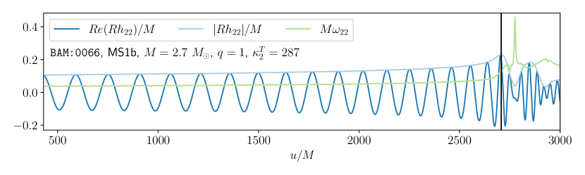
Figure 6: The real part of the strain $Rh_{22}$, its amplitude $|Rh_{22}|$, and frequency $M\omega_{22}$ of BAM:0066. The black solid line indicates the moment of merger.

In this section we present a waveform error analysis for BAM:0066 [20]. This example effectively represents data that exhibit second order convergence. Figure 6 shows the strain $Rh_{22}$ at the lowest extraction radius available for this simulation, $R=700\,{\rm M_{\odot}}$, its amplitude $|Rh_{22}|$ and frequency $M\omega_{22}$. Note that in this section we use $R$ instead of $D_{L}$.

In order to test self-convergence, we compare amplitude and phase differences of $R\psi_{22}$ between the different resolutions. For this case, we consider the simulation at resolutions $n_{m}=120,160,240$ grid points on the highest refined AMR level; hereafter Low (L), Medium (M), and High (H). The convergence rate $p$ is found experimentally by rescaling these differences using the scaling factor ${\rm SF}$ [172],

$${\rm SF}=\frac{\Delta^{p}_{\rm L}-\Delta^{p}_{\rm M}}{\Delta^{p}_{\rm M}-\Delta^{p}_{\rm H}}$$ (20)

where $\Delta_{x}$ is the grid spacing at resolution $x$. We show the self-convergence test in Figure 7. The differences decrease with increasing resolution, as one would expect from convergent data. They also increase with increasing simulation time because truncation errors accumulate during the simulation. The optimal scaling is found for $p=2$ with ${\rm SF}(2)=1.4$, thus indicating second order convergence. In presence of convergence, a measure of the error to be assigned to the (highest resolution) data is given simply by the difference between the two highest resolutions. This is a conservative estimate because (for convergent data) the truncation error is certainly smaller. Alternatively, the experimental convergence factor can be in principle used in a Richardson extrapolation of the data to provide an improved dataset and error estimate [172, 19]. Note that in this procedure the waveforms are not shifted by a relative time and phase shift because the simulations of the convergent series are run using the same initial data with a fixed initial phase.

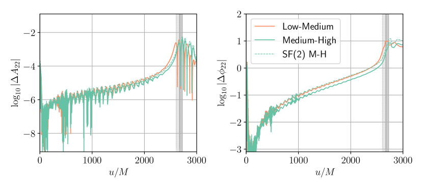
Figure 7: Self-convergence tests of BAM:0066 $R\psi_{22}$ The dashed blue line represents the rescaled difference for second order convergence. The light (dark) gray shaded regions show the time of merger differences of Low-Medium (Medium-High) resolutions.

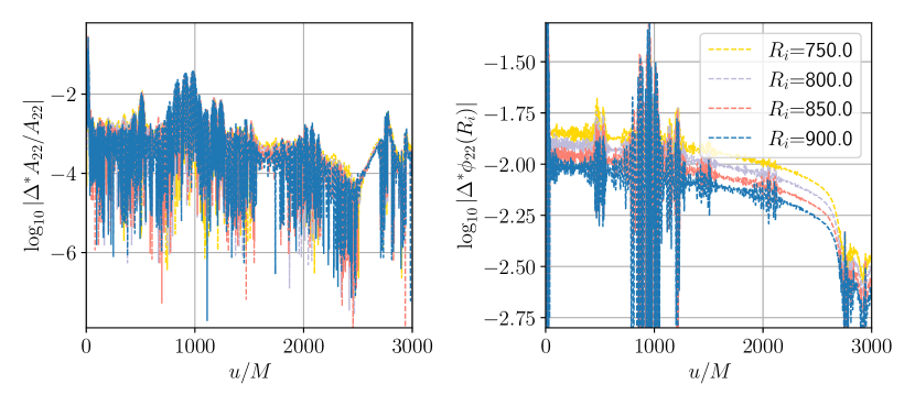
Figure 8: Amplitude (left) and phase (right) differences between BAM:0066’s $R\psi_{22}$ extracted at consecutive finite-radii $R_{i}=700,750,800,850,900~{}{\rm M_{\odot}}$.

To assess the uncertainties originated from the waveform obtained at finite-extraction radii, $R_{i}$, we compare the phase differences between consecutive radii [172]

$$\Delta^{*}\phi_{22}(R_{i})=\phi_{22}(R_{i})-\phi_{22}(R_{i-1})\,,$$ (21)

and similarly for the relative amplitudes, $\Delta^{*}A_{22}/A_{22}$. In Fig. 8 we show the differences at the extraction radii $R=700,750,800,850,900~{}{\rm M_{\odot}}$. The phase differences decrease at progressively large radii, thus indicating the numerical waveforms are converging towards their true morphology at null infinity. The phase differences are larger at early times and decrease towards merger; note this behaviour has the opposite sign of that of resolution effects [19]. The relative differences in amplitude are ${\sim}10^{-4}$ for all radii, indicating robust results are obtained already with relatively close extraction sphere. The waveforms can be extrapolated to null infinity using either a polynomial in $1/R$ of order $K$ [172] or the method outline in [183]. The two methods give comparable results; the former is more general and can be applied to the curvature multipoles $\psi_{\ell m}$, the latter is a simpler method for the strain modes. An error due to finite extraction can be then assigned to the data at finite extraction as the difference with the extrapolated data (or viceversa). Another method is to post-process simulations using Cauchy characteristic extraction (CCE) [184] and to simulate the waveform at future null infinity. This technique was used for some of the CoRe data.

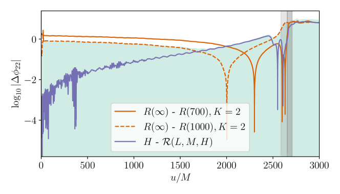
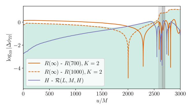
Figure 9: Error budget (shown as a green shaded area) for the phase of $R\psi^{4}_{22}$ (top) and $Rh_{22}$ (bottom) from the truncation error (blue line) and finite-radius extraction uncertainty (orange lines) employing polynomial extrapolation with $K=2$. The blue line shows the difference between the highest resolution and the Richardson extrapolated dataset $\mathcal{R}(L,M,H)$.

The total error budget can be computed as the sum in quadrature of the truncation and finite extraction errors, and it is shown in Fig. 9 for both the curvature and strain (2,2) modes. As mentioned above, the truncation phase error is typically a factor ${\sim}2$ larger than the finite extraction error (for $R\gtrsim 500{\rm M_{\odot}}$) at merger and in simulations with tens of orbits.

Finally, we obtain the unfaithfulness $\bar{\mathcal{F}}$ of the waveforms between the different resolutions (M-H and L-M). The Wiener integral is evaluated in the frequency range $f\in[f_{\rm min},f_{\rm mrg}]$ and employing the Advanced LIGO PSD P1200087 [185] from bajes [186]. Here $f_{\rm min}$ corresponds to the initial GW frequency, and $f_{\rm mrg}$ to the frequency at the moment of merger. For the faithfulness threshold $\mathcal{F}_{\rm thr}$ in Eq. (19), we consider $\epsilon^{2}=1$ as the strict requirement, and $\epsilon^{2}=6$, corresponding to the number of intrinsic parameters of a BNS. Similarly to [65], the SNR values are chosen to be $\rho=14,30,80$. Figure 10 shows the computed values. The smallest unfaithfulness (M-H, $n_{m}=240,160$) passes five out of the six accuracy tests, whereas the other one (L-M, $n_{m}=160,120$) passes only two, namely $\mathcal{F}^{14,6}_{\rm thr}$ and $\mathcal{F}^{30,6}_{\rm thr}$. However, the unfaithfulness value lies closely (or on top) of the threshold $\mathcal{F}^{14,1}_{\rm thr}$.

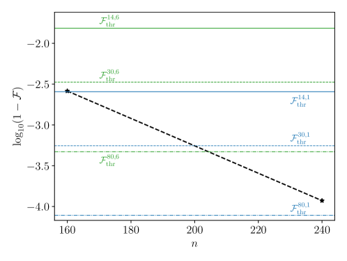
Figure 10: Unfaithfulness of BAM:0066’s Medium-High ($n_{m}=240,160$) and Low-Medium ($n_{m}=160,120$) $Rh_{22}$ waveforms. The blue and green lines represent the accuracy tests $\mathcal{F}^{\rho,\epsilon^{2}}_{\rm thr}$ for different values of $\rho$ (SNR) and $\epsilon^{2}$.

Analyses similar to the one above are necessary to determine the quality of the NR data for GW modelling. Convergence of the data is a necessary requisite for robust error estimates. Other diagnostic quantities used to verify convergence in simulations are constraint violation, baryon mass conservation and the stars oscillations during the first orbits, e.g. [101, 172, 98, 81, 60]. Achieving waveform convergence in long-term evolutions of BNS is a nontrivial result and, in our experience, requires at least fifth order finite-differencing schemes or finite volume schemes with fifth order reconstructions (at the current resolutions) [104, 19, 65]. Second [19], approximately third [104] and clear fourth order convergence [65] has been demonstrated up to merger in some data using these finite-differencing conservative schemes. Extreme mass ratios $q\sim 2$ and NS rotation close to the breakup limit remain challenging to simulate as well as to obtain clean convergence in GW higher (subdominant) modes like $(\ell,m)=(2,1),(3,3)$ and $(4,4)$. Work in these directions is ongoing [58, 62, 64, 65]. For example, clear fourth order convergence in the subdominant (3, 2) and (4, 4) modes for $q=1$ has been shown in [65]. Postmerger waveforms typically show slower convergence due to shock formation at merger and the complex fluid dynamics in the remnant. Nonetheless, GW spectra have remarkably robust features that can be accurately quantified with NR data, as we shall discuss in Sec. 5. We refer the reader to Ref. [33, 38] for recent work on the accuracy of CoRe postmerger waveform.

4.2 Faithfulness analysis

In an attempt to give an overview of the accuracy of the waveform database, we compute the unfaithfulness of the (2,2) mode waveforms $h_{22}$ between the highest and second highest resolutions, for the whole database. We use again the zero-detuned, high-power Advanced LIGO PSD [185]. The minimum frequency $f_{\rm min}$ employed in the integral of Eq. (17) corresponds to the initial frequency of each individual simulation.

The result of this analysis is summarized in Fig. 11, where $\bar{\mathcal{F}}$ is shown as a function of the number of orbits and different colors mark the microphysics scheme employed in each simulation. The unfaithfulness values are scattered on a wide range, but about 65% of the waveforms lay below the 1% level which is conventionally considered the accuracy threshold for detection purposes. Importantly, the dependence on the number of orbits (simulation length) is very weak and most of the simulations with ten or more orbits have $\bar{\mathcal{F}}<0.01$. Several waveforms from multiple-orbits have $\bar{\mathcal{F}}\lesssim 10^{-4}$; according to the analysis in the previous section, these data can be considered faithful (suitable for parameter estimation) up to signal SNR of 30-80. We note that data with very few orbits (e.g. THC:0019, BAM:0029, and BAM:0082) show a remarkably low unfaithfulness. These simulations have a short inspiral and rather focus on the postmerger signal, which is not considered in this analysis. Hence, small $\bar{\mathcal{F}}$ is not necessarily an indication that these simulations are suitable for waveform modelling.

A faithfulness analysis for postmerger signals was recently presented by some of us in [33, 38]. There, we found average mismatches of ${\sim}0.01-0.4$. The main source of uncertainty in the postmerger waveforms is the numerical resolution (see the above Section) and the impact of the resolution on the remnant’s collapse.

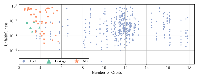
Figure 11: Unfaithfulness computed between the highest and second highest simulations $h_{22}$ waveforms for every configuration of the database. The different colors and markers correspond to the microphysics scheme employed for each simulation.

5 Quasi-universal relations

Table 2: Updated fit coefficients for relevant merger and PM quantities.

$Q^{\rm fit}$	$a_{0}$	$k$	$a^{M}_{k}$	$a^{S}_{k}$	$b^{S}_{k}$	$a^{T}_{k}$	$b^{T}_{k}$	$\chi^{2}$	Error	$R^{2}$
$A_{\rm mrg}/M$	0.55	1	5.27	0.31	-39.21	5.59$\times 10^{-2}$	-2.51$\times 10^{-2}$	0.113	2.6%	0.949
		2				1.00$\times 10^{-6}$	-2.00
		3				0.12	11.09
		4				6.79$\times 10^{-5}$	9.72
$Mf_{\rm mrg}/\nu$	0.22	1	0.80	0.25	-1.99	4.85$\times 10^{-2}$	1.80	0.329	4.5%	0.925
		2				5.86$\times 10^{-6}$	599.99
		3				0.1	7.80
		4				1.86$\times 10^{-4}$	84.76
$Mf_{2}$	8.99$\times 10^{-2}$	1	31.02	7.42$\times 10^{-2}$	29.99	2.94$\times 10^{-2}$	1.13	0.067	3.6%	0.958
		2				3.78$\times 10^{-5}$	-0.99
		3				5.75$\times 10^{-2}$	39.99
		4				2.77$\times 10^{-4}$	27.77

Table 3: Updated fit coefficients for $Mf_{2}$ as a function of the NS radii $R_{1.4}$ and $R_{1.8}$.

	$a_{0}$	$a_{1}$	$a_{2}$	$a_{3}$	$\chi^{2}$	Error	$R^{2}$
$Mf_{2}(R_{1.4}/M)$	0.24	-0.10	1.13$\times 10^{-2}$	-	0.55	5.9$\%$	0.901
$Mf_{2}(R_{1.8}/M)$	0.23	-0.10	1.21$\times 10^{-2}$	-	0.31	4.5$\%$	0.949
$Mf_{2}(R_{1.4}/M,R_{1.4}/R_{1.8})$	0.15	-0.11	1.38$\times 10^{-2}$	9.76$\times 10^{-2}$	0.31	4.5$\%$	0.949
$Mf_{2}(R_{1.8}/M,R_{1.4}/R_{1.8})$	0.20	-0.10	1.22$\times 10^{-2}$	2.77$\times 10^{-2}$	0.30	4.4$\%$	0.952

Table 4: Best fit coefficients for the luminosity peak. The last columns show the $\chi^{2}$, the fit’s relative standard deviation and the coefficient of determination $R^{2}$.

	$k$	$p_{k10}$	$p_{k11}$	$p_{k20}$	$p_{k21}$	$p_{k30}$	$p_{k31}$	$\chi^{2}$	Error	$R^{2}$
	1	2.28	7.59$\times 10^{-1}$	-17.74	-0.57	-17.47	4.58
$L_{\rm peak}/\nu$	2	-8.38$\times 10^{-2}$	9.61$\times 10^{-3}$	3.24$\times 10^{-1}$	-3.33$\times 10^{-2}$	13.91	10.10	2.23	12%	0.961
	3	-5.18$\times 10^{-1}$	14.64	-5.35	-50.54	11.61	-29.96

As a first application of the database, we present in this section new EOS-insensitive relations for the merger and postmerger waveforms. Previous work found that several key quantities characterizing the merger dynamics depend on the unknown EOS mainly throughout the tidal parameters and have a very weak dependence on other details of the matter model, e.g., [153, 187, 188, 29, 189, 150, 58]. Similarly, the GW postmerger spectrum has robust features that can be captured within a few percent accuracy by tidal parameters and/or other properties of NS equilibria in EOS-insensitive way [153, 27, 154, 28, 33, 155]. These relations have some practical use in GW astronomy because they deliver accurate estimates for the peak luminosity [150, 53] and for the remnant properties [190, 191, 192] (see also [53] for a detailed review) and because they are the building blocks to develop NR-informed waveform models.

First, we consider the mass-rescaled GW amplitude and frequency at the moment of merger, $A^{\rm mrg}_{22}/M$ and $Mf^{\rm mrg}_{22}/\nu$, and update the fits developed in Ref. [188, 33, 38]. Following closely the fitting procedure of Ref. [38], we represent any quantity by the factorized function

$$Q^{\rm fit}=a_{0}Q^{M}(X)Q^{S}(\hat{S},X)Q^{T}(\kappa^{T}_{2},X)\,,$$ (22)

where each factor $Q^{M}$, $Q^{S}$, $Q^{T}$ accounts for the mass ratio in terms of $X=1-4\nu$, spin corrections in terms of $\hat{S}$, and tidal effects in terms of $\kappa^{T}_{2}$. The first two factors are given by the linear polynomial expressions $Q^{M}=1+a^{M}_{1}X$, and $Q^{S}=1+p^{S}_{1}\hat{S}$, with $p^{S}_{1}=a^{S}_{1}(1+b^{S}_{1}X)$. The last factor is instead a rational polynomial

$$Q^{T}=\frac{1+p^{T}_{1}\kappa^{T}_{2}+p^{T}_{2}{\kappa^{T}_{2}}^{2}}{1+p^{T}_{3}\kappa^{T}_{2}+p^{T}_{4}{\kappa^{T}_{2}}^{2}}\,,$$ (23)

with $p^{T}_{i}=a^{T}_{i}(1+b^{T}_{i}X)$. The best fit parameters are shown in Tab. 4. The amplitude and frequency have $1\sigma$ errors of $2.6\%$ and $4.6\%$ respectively. We also obtain a $\chi^{2}$ of $\sim 0.126$ for the former and $\sim 0.329$ for the latter.

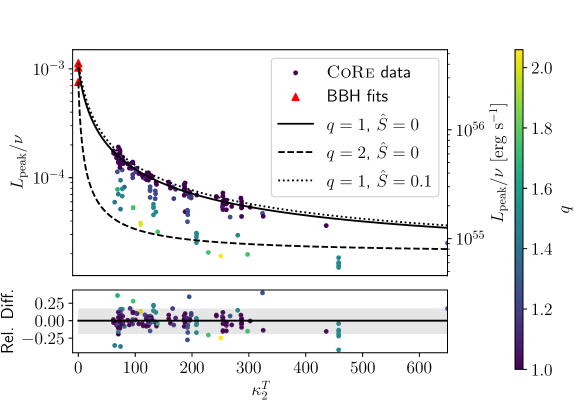
Figure 12: Luminosity peak data from the CoRe database. Black lines show the new fits developed for different mass ratio and spin configurations. The relative differences are shown in the bottom panel, where the gray shaded region marks the $90\%$ credible region.

Next, we use the public CoRe data on the emitted GW energy and extract the peak luminosity $L_{\rm peak}$ using Eq. (12). For binary black holes, this quantity does not depend on the mass scale and it is accurately described by the fits of Ref. [193]. For BNS, it has been studied in Ref. [150]. We propose the ansatz

$$L_{\rm peak}(\nu,\,\hat{S},\,\kappa^{T}_{2})/\nu=L^{\rm BBH}_{\rm peak}\frac{1+p_{1}(\nu,\,\hat{S})\kappa^{T}_{2}+p_{2}(\nu,\,\hat{S}){\kappa^{T}_{2}}^{2}}{(1+[p_{3}(\nu,\,\hat{S})]^{2}\kappa^{T}_{2})^{2}}\,,$$ (24)

where $L^{\rm BBH}_{\rm peak}$ are the mass and spin dependent fits from Ref. [193] and

$$p_{k}(\nu,\,\hat{S}) =p_{k1}(\hat{S})\nu+p_{k2}(\hat{S})\nu^{2}+p_{k3}(\hat{S})\nu^{3}$$

$$p_{kj}(\hat{S}) =p_{kj0}\hat{S}+p_{kj1}\,.$$

Note the scaling factor $1/\nu$ for $L_{\rm peak}$. By construction, the fit reduces to the BBH case for $\kappa^{T}_{2}\rightarrow 0$. The luminosity peak is calculated in geometric units; the conversion factor to CGS units is given by the Planck luminosity $L_{P}=c^{5}/G\approx 3.63\times 10^{59}~{}\rm{erg}~{}\rm{s}^{-1}$. Figure 12 shows the best fit for $L_{\rm peak}/\nu$ and the CoRe data; the best fitting coefficients are reported in Tab. 4. The average $1\sigma$ deviation is about $12\%$ over the entire dataset with less than a dozen of outliers. The peak luminosities for $q\sim 2$ BNS are the least accurately modelled (4 BNS configurations). The figure shows that the largest peak luminosities are reached by BNS with $\kappa^{\rm T}_{2}\lesssim 80$ that correspond to high-mass binaries and prompt collapse mergers. These events can reach peak luminosities of ${\sim}10^{55}~{}\rm{erg}~{}\rm{s}^{-1}$, about an order of magnitude less than binary black holes (of any mass). BNS mass ratios $q\gtrsim 1.5$ can lower $L_{\rm peak}$ of about an order of magnitude, while spins of magnitude ${\sim}0.1$ do not significantly affect $L_{\rm peak}$. We stress that BNS with the largest peak luminosity do not correspond in general to the BNS that radiate the largest amount of energy because postmerger emission can radiate further energy [149, 150] (see also Fig. 5). We can set an upper limit to the total radiated GW energy from our dataset, obtaining $E^{\rm tot}_{\rm GW}\lesssim 0.676~{}{\rm M_{\odot}}c^{2}$.

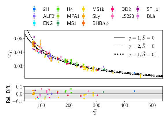
Figure 13: Quasi-universal relation of the post-merger peak frequency $Mf_{2}$ (mass rescaled) as a function of the tidal polarizability $\kappa^{T}_{2}$. Each point represents a simulation of the CoRe database with its corresponding EOS (in different colors). Black lines represent the updated $Mf_{2}$-fits (top panel). The relative differences are shown in the bottom panel, where the gray shaded region marks the $90\%$ credible region.

Finally, we illustrate the use of CoRe data to model postmerger GWs by discussing a fit of the postmerger’s spectrum peak frequency $f_{2}$, e.g. [29, 28, 33, 38]. This peak frequency is a robust feature found in all NR simulations. Direct GW inference on $f_{2}$ can be used to constrain NS properties [190, 154, 191, 194, 34, 32, 155]. The peak frequency also enters as one of the central parameters in postmerger waveform models that will be employed in the future for more sophisticated matched-filter analyses [195]. Following Ref. [38] we employ again Eq. (22) to fit the mass-rescaled $Mf_{2}$. The best fitting coefficients are presented in Table 4 and have a $\chi^{2}\sim 0.07$. Figure 13 shows $Mf_{2}$ as a function of $\kappa^{\rm T}_{2}$ for selected values of mass ratio and spin. The $1\sigma$ error is below $4\%$; this precision is in principle sufficient for informative measurements of the NS mass-radius sequence. For example, using the EOS-insensitive relation between $f_{2}$ and the maximum density of an equilibrium non-rotating NS put forward in [155], it would be possible to determine the maximum density of an equilibrium non-rotating NS to ${\sim}15\%$ and the maximum mass ${M_{\rm max}^{\rm TOV}}$ to ${\sim}12\%$ with a single signal at the detectability threshold.

As a further illustration, we calibrate the EOS-insensitive relations (mass-rescaled) between $f_{2}$ and the NS radius [196, 197, 38]

$$Mf_{2}\left(\frac{R_{X}}{M}\right)=a_{0}+a_{1}\frac{R_{X}}{M}+a_{2}\left(\frac{R_{X}}{M}\right)^{2}$$

$$Mf_{2}\left(\frac{R_{X}}{M},\frac{R_{1.4}}{R_{1.8}}\right)=a_{0}+a_{1}\frac{R_{X}}{M}+a_{2}\left(\frac{R_{X}}{M}\right)^{2}+a_{3}\frac{R_{1.4}}{R_{1.8}}\,,$$ (25)

where $R_{X}$ is the equilibrium radius corresponding to a NS with mass $X=1.4,\,1.8~{}{\rm M_{\odot}}$. Figure 14 shows $Mf_{2}$ as function of $R_{1.4}$, $R_{1.8}$ and $R_{1.4}/R_{1.8}$. Best fit parameters are given in Table 4. Other features of the postmerger spectrum can be quantified in a similar way. We release reduced postmerger data and analysis scripts on the CoRe website.

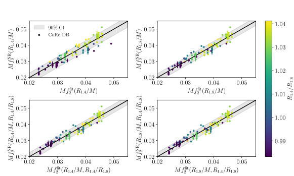
Figure 14: Quasi-universal relation of the post-merger peak frequency $Mf_{2}$ (mass rescaled) as a function of the NS radius $R_{1.4}$, $R_{1.8}$. Each point represents a simulation of the CoRe database with the different colors representing the ratio $R_{1.4}/R_{1.8}$. Each panel shows the different fit calibrations performed in [38]. The black line represents the case when $Mf_{2}^{\rm{NR}}=Mf_{2}^{\rm{fit}}$, whereas the gray area shows the $90\%$ credibility level.

6 Conclusion

We presented a new set of BNS simulations for the second release of the CoRe database, expanding it to 254 different binary configurations covering a wide parameter space. The new data includes BNS consistent with the GW events GW170817 [59] and GW190425 [68, 66]. Simulations were performed with a large number of EOSs, including several microphysical models [66, 59, 63]. Some simulations include the effects of neutrinos, either through the leakage scheme [133, 198, 106], or using the M0 approach [106, 54]. Turbulent viscosity is included in some models using the GRLES formalism [108, 61]. Finally, we include simulations produced using a new hybrid numerical flux scheme, EFL, that was introduced in [65] showing fourth order convergence and smaller phase errors than previous simulations using WENO schemes in BAM.

We described in detail the methodology we used to assess the overall accuracy of the waveforms and presented results for all the configurations in the database. The CoRe database waveform have typical unfaithfulness of less than $10^{-2}$, some have unfaithfulness of less than $10^{-4}$, so they are suitable for precision waveform modelling applications. However, to ensure the convergence and usability of the simulations, more extensive analysis is needed. As an example, we showed a full analysis of one of our simulations, BAM:0066, which showed a clear second order convergence and passed several accuracy tests.

Finally, as a first application of the CoRe database, we fitted phenomenological formulas for the merger amplitude, frequency, and GW luminosity. These fits are able to model the CoRe data with high accuracy ($<5\%$ for the merger amplitude and frequency and $17\%$ for the peak luminosity). We also recalibrated various quasi-universal relations between the post-merger peak frequency and the binary parameters, again finding deviations from the universal relations of only a few percent. These were used in [38] to construct the first complete inspiral, merger, and post-merger waveform model for BNS.

We release the CoRe database to the community with the hope that it will enable future discoveries in GW astronomy. Potential applications include the development of new waveform models, the validation of data analysis pipelines and new numerical relativity codes, and the planning of future GW experiments. In the future, we plan to release new simulation data on a rolling basis, with data releases taking place at the publication time of the corresponding paper.

References

Appendix A Public CoRe Database

The simulation data discussed in this work is publicly available at

http://www.computational-relativity.org/gwdb/

The database metadata are summarized in the repo core-database-index, which contains a json file with the main properties of the available simulations and the different runs. A repository is associated to one distinct physical binary and contains folders for the different runs performed. For each run, we release a complete metadata file and a HDF5 file with the multipolar waveform for both $\psi_{\ell m}$ and $h_{\ell m}$ at different extraction radii and the energetics.

Access to our private codes and data is possible upon reasonable request. Any use of the simulation data must be done in accordance with the terms of use contained here: http://www.computational-relativity.org/terms/.

Appendix B watpy: Waveform Analysis Tools in Python

The repository

https://git.tpi.uni-jena.de/core/watpy

provides classes to work with the CoRe waveforms and tutorials. It is also available via PyPI

https://pypi.org/project/core-watpy/.

The code includes two main modules. The coredb module contains tools to download and upload NR simulation data, menage the metadata of the simulations, visualize statistics of the database, and work with the HDF5 files provided in the CoRe website. The wave module provides methods for the visualization and the analysis of (multipolar) NR outputs, i.e. Weyl curvature and GW strain. watpy  is compatible with NR files from BAM, Cactus/Einstein Toolkit (WhiskyTHC/FreeTHC) and the CoRe database.

Appendix C Merger and postmerger fit data

The data and scripts employed for the development of the fits presented in this work, can be found in

https://doi.org/10.5281/zenodo.7253784.

Any reuse of the merger and postmerger fit data must be done in accordance with the Creative Commons Attribution 4.0 International license which applies to the data files.

Appendix D THC

THC is open source and publicly available At

https://bitbucket.org/FreeTHC/workspace/projects/THC

A tutorial, microphysics tables, and example parfiles are available at

http://personal.psu.edu/~dur566/whiskythc.html

References

- [1] Mroue A H, Scheel M A, Szilagyi B, Pfeiffer H P, Boyle M et al. 2013 Phys.Rev.Lett. 111 241104 (Preprint 1304.6077)
- [2] Chu T, Fong H, Kumar P, Pfeiffer H P, Boyle M, Hemberger D A, Kidder L E, Scheel M A and Szilagyi B 2016 Class. Quant. Grav. 33 165001 (Preprint 1512.06800)
- [3] Boyle M et al. 2019 Class. Quant. Grav. 36 195006 (Preprint 1904.04831)
- [4] Healy J, Lousto C O, Zlochower Y and Campanelli M 2017 Class. Quant. Grav. 34 224001 (Preprint 1703.03423)
- [5] Healy J, Lousto C O, Lange J, O’Shaughnessy R, Zlochower Y and Campanelli M 2019 Phys. Rev. D 100 024021 (Preprint 1901.02553)
- [6] Healy J and Lousto C O 2020 Phys. Rev. D 102 104018 (Preprint 2007.07910)
- [7] Jani K, Healy J, Clark J A, London L, Laguna P and Shoemaker D 2016 Class. Quant. Grav. 33 204001 (Preprint 1605.03204)
- [8] Dietrich T, Radice D, Bernuzzi S, Zappa F, Perego A, Brügmann B, Chaurasia S V, Dudi R, Tichy W and Ujevic M 2018 Class. Quant. Grav. 35 24LT01 (Preprint 1806.01625)
- [9] Kiuchi K, Kawaguchi K, Kyutoku K, Sekiguchi Y, Shibata M and Taniguchi K 2017 Phys. Rev. D96 084060 (Preprint 1708.08926)
- [10] Kiuchi K, Kyohei K, Kyutoku K, Sekiguchi Y and Shibata M 2019 (Preprint 1907.03790)
- [11] Foucart F et al. 2019 Phys. Rev. D 99 044008 (Preprint 1812.06988)
- [12] Gravitational Wave Signal Catalog https://stellarcollapse.org/gwcatalog.html
- [13] BNS waveforms https://bitbucket.org/ciolfir/bns-waveforms
- [14] Baiotti L, Damour T, Giacomazzo B, Nagar A and Rezzolla L 2011 Phys. Rev. D84 024017 (Preprint 1103.3874)
- [15] Bernuzzi S, Nagar A, Thierfelder M and Brügmann B 2012 Phys.Rev. D86 044030 (Preprint 1205.3403)
- [16] Bernuzzi S, Nagar A, Dietrich T and Damour T 2015 Phys.Rev.Lett. 114 161103 (Preprint 1412.4553)
- [17] Hinderer T et al. 2016 Phys. Rev. Lett. 116 181101 (Preprint 1602.00599)
- [18] Steinhoff J, Hinderer T, Buonanno A and Taracchini A 2016 Phys. Rev. D94 104028 (Preprint 1608.01907)
- [19] Bernuzzi S and Dietrich T 2016 Phys. Rev. D94 064062 (Preprint 1604.07999)
- [20] Dietrich T, Bernuzzi S and Tichy W 2017 Phys. Rev. D96 121501 (Preprint 1706.02969)
- [21] Kawaguchi K, Kiuchi K, Kyutoku K, Sekiguchi Y, Shibata M and Taniguchi K 2018 Phys. Rev. D97 044044 (Preprint 1802.06518)
- [22] Nagar A et al. 2018 Phys. Rev. D98 104052 (Preprint 1806.01772)
- [23] Nagar A, Messina F, Rettegno P, Bini D, Damour T, Geralico A, Akcay S and Bernuzzi S 2019 Phys. Rev. D99 044007 (Preprint 1812.07923)
- [24] Akcay S, Bernuzzi S, Messina F, Nagar A, Ortiz N and Rettegno P 2019 Phys. Rev. D99 044051 (Preprint 1812.02744)
- [25] Isoyama S, Sturani R and Nakano H 2020 (Preprint 2012.01350)
- [26] Gamba R, Akçay S, Bernuzzi S and Williams J 2022 Phys. Rev. D 106 024020 (Preprint 2111.03675)
- [27] Hotokezaka K, Kiuchi K, Kyutoku K, Muranushi T, Sekiguchi Y i et al. 2013 Phys.Rev. D88 044026 (Preprint 1307.5888)
- [28] Bernuzzi S, Dietrich T and Nagar A 2015 Phys. Rev. Lett. 115 091101 (Preprint 1504.01764)
- [29] Bauswein A and Stergioulas N 2015 Phys. Rev. D91 124056 (Preprint 1502.03176)
- [30] Clark J A, Bauswein A, Stergioulas N and Shoemaker D 2016 Class. Quant. Grav. 33 085003 (Preprint 1509.08522)
- [31] Easter P J, Lasky P D, Casey A R, Rezzolla L and Takami K 2019 Phys. Rev. D 100 043005 (Preprint 1811.11183)
- [32] Tsang K W, Dietrich T and Van Den Broeck C 2019 Phys. Rev. D100 044047 (Preprint 1907.02424)
- [33] Breschi M, Bernuzzi S, Zappa F, Agathos M, Perego A, Radice D and Nagar A 2019 Phys. Rev. D100 104029 (Preprint 1908.11418)
- [34] Easter P J, Ghonge S, Lasky P D, Casey A R, Clark J A, Vivanco F H and Chatziioannou K 2020 Phys. Rev. D 102 043011 (Preprint 2006.04396)
- [35] Soultanis T, Bauswein A and Stergioulas N 2022 Phys. Rev. D 105 043020 (Preprint 2111.08353)
- [36] Wijngaarden M, Chatziioannou K, Bauswein A, Clark J A and Cornish N J 2022 (Preprint 2202.09382)
- [37] Whittaker T, East W E, Green S R, Lehner L and Yang H 2022 (Preprint 2201.06461)
- [38] Breschi M, Bernuzzi S, Chakravarti K, Camilletti A, Prakash A and Perego A 2022 (Preprint 2205.09112)
- [39] Abbott B P et al. (Virgo, LIGO Scientific) 2017 Astrophys. J. 851 L16 (Preprint 1710.09320)
- [40] Abbott B P et al. (LIGO Scientific, Virgo) 2019 Phys. Rev. X9 011001 (Preprint 1805.11579)
- [41] Abbott B P et al. (LIGO Scientific, Virgo) 2018 Phys. Rev. Lett. 121 161101 (Preprint 1805.11581)
- [42] Abbott B P et al. (LIGO Scientific, Virgo) 2020 Class. Quant. Grav. 37 045006 (Preprint 1908.01012)
- [43] Shibata M, Taniguchi K and Uryu K 2005 Phys. Rev. D71 084021 (Preprint gr-qc/0503119)
- [44] Shibata M and Taniguchi K 2006 Phys.Rev. D73 064027 (Preprint astro-ph/0603145)
- [45] Hotokezaka K, Kyutoku K, Okawa H, Shibata M and Kiuchi K 2011 Phys.Rev. D83 124008 (Preprint 1105.4370)
- [46] Bernuzzi S, Dietrich T, Tichy W and Brügmann B 2014 Phys.Rev. D89 104021 (Preprint 1311.4443)
- [47] Dietrich T, Ujevic M, Tichy W, Bernuzzi S and Brügmann B 2017 Phys. Rev. D95 024029 (Preprint 1607.06636)
- [48] Dietrich T, Bernuzzi S, Ujevic M and Tichy W 2017 Phys. Rev. D95 044045 (Preprint 1611.07367)
- [49] Dietrich T, Bernuzzi S, Brügmann B, Ujevic M and Tichy W 2018 Phys. Rev. D97 064002 (Preprint 1712.02992)
- [50] Köppel S, Bovard L and Rezzolla L 2019 Astrophys. J. 872 L16 (Preprint 1901.09977)
- [51] Baumgarte T W, Shapiro S L and Shibata M 2000 Astrophys. J. 528 L29 (Preprint astro-ph/9910565)
- [52] Radice D, Bernuzzi S and Perego A 2020 Ann. Rev. Nucl. Part. Sci. 70 (Preprint 2002.03863)
- [53] Bernuzzi S 2020 Gen. Rel. Grav. 52 108 (Preprint %****␣paper20230323.bbl␣Line␣225␣****2004.06419)
- [54] Radice D, Perego A, Hotokezaka K, Fromm S A, Bernuzzi S and Roberts L F 2018 Astrophys. J. 869 130 (Preprint 1809.11161)
- [55] Perego A, Bernuzzi S and Radice D 2019 Eur. Phys. J. A55 124 (Preprint 1903.07898)
- [56] Endrizzi A, Perego A, Fabbri F M, Branca L, Radice D, Bernuzzi S, Giacomazzo B, Pederiva F and Lovato A 2020 Eur. Phys. J. A 56 15 (Preprint 1908.04952)
- [57] Poudel A, Tichy W, Brügmann B and Dietrich T 2020 Phys. Rev. D 102 104014 (Preprint 2009.06617)
- [58] Bernuzzi S et al. 2020 Mon. Not. Roy. Astron. Soc. (Preprint 2003.06015)
- [59] Nedora V, Bernuzzi S, Radice D, Daszuta B, Endrizzi A, Perego A, Prakash A, Safarzadeh M, Schianchi F and Logoteta D 2021 Astrophys. J. 906 98 (Preprint 2008.04333)
- [60] Chaurasia S V, Dietrich T, Ujevic M, Hendriks K, Dudi R, Fabbri F M, Tichy W and Brügmann B 2020 Phys. Rev. D 102 024087 (Preprint 2003.11901)
- [61] Radice D 2020 Symmetry 12 1249 (Preprint 2005.09002)
- [62] Dudi R, Adhikari A, Brügmann B, Dietrich T, Hayashi K, Kawaguchi K, Kiuchi K, Kyutoku K, Shibata M and Tichy W 2021 (Preprint 2109.04063)
- [63] Prakash A, Radice D, Logoteta D, Perego A, Nedora V, Bombaci I, Kashyap R, Bernuzzi S and Endrizzi A 2021 Phys. Rev. D 104 083029 (Preprint 2106.07885)
- [64] Ujevic M, Rashti A, Gieg H, Tichy W and Dietrich T 2022 (Preprint 2202.09343)
- [65] Doulis G, Atteneder F, Bernuzzi S and Brügmann B 2022 Phys. Rev. D 106 024001 (Preprint 2202.08839)
- [66] Camilletti A, Chiesa L, Ricigliano G, Perego A, Lippold L C, Padamata S, Bernuzzi S, Radice D, Logoteta D and Guercilena F M 2022 (Preprint 2204.05336)
- [67] Perego A, Radice D and Bernuzzi S 2017 Astrophys. J. 850 L37 (Preprint 1711.03982)
- [68] Dudi R, Pannarale F, Dietrich T, Hannam M, Bernuzzi S, Ohme F and Bruegmann B 2018 (Preprint 1808.09749)
- [69] Nagar A, Pratten G, Riemenschneider G and Gamba R 2019 (Preprint 1904.09550)
- [70] Damour T and Nagar A 2010 Phys. Rev. D81 084016 (Preprint 0911.5041)
- [71] Favata M 2014 Phys.Rev.Lett. 112 101101 (Preprint 1310.8288)
- [72] Reisswig C and Pollney D 2011 Class.Quant.Grav. 28 195015 (Preprint 1006.1632)
- [73] Damour T, Nagar A, Hannam M, Husa S and Brügmann B 2008 Phys. Rev. D78 044039 (Preprint 0803.3162)
- [74] Baiotti L, Bernuzzi S, Corvino G, De Pietri R and Nagar A 2009 Phys. Rev. D79 024002 (Preprint 0808.4002)
- [75] Damour T, Nagar A, Pollney D and Reisswig C 2012 Phys.Rev.Lett. 108 131101 (Preprint 1110.2938)
- [76] York James W J 1999 Phys.Rev.Lett. 82 1350–1353 (Preprint gr-qc/9810051)
- [77] Wilson J and Mathews G 1995 Phys.Rev.Lett. 75 4161–4164
- [78] Wilson J, Mathews G and Marronetti P 1996 Phys.Rev. D54 1317–1331 (Preprint gr-qc/9601017)
- [79] Tichy W 2011 Phys.Rev. D84 024041 (Preprint 1107.1440)
- [80] Tichy W 2012 Phys. Rev. D 86 064024 (Preprint 1209.5336)
- [81] Dietrich T, Moldenhauer N, Johnson-McDaniel N K, Bernuzzi S, Markakis C M, Brügmann B and Tichy W 2015 Phys. Rev. D92 124007 (Preprint 1507.07100)
- [82] Tacik N et al. 2015 Phys. Rev. D92 124012 [Erratum: Phys. Rev.D94,no.4,049903(2016)] (Preprint 1508.06986)
- [83] Tichy W, Rashti A, Dietrich T, Dudi R and Brügmann B 2019 Phys. Rev. D100 124046 (Preprint 1910.09690)
- [84] Moldenhauer N, Markakis C M, Johnson-McDaniel N K, Tichy W and Brügmann B 2014 Phys. Rev. D90 084043 (Preprint 1408.4136)
- [85] Tichy W 2009 Phys.Rev. D80 104034 (Preprint 0911.0973)
- [86] Pfeiffer H P, Brown D A, Kidder L E, Lindblom L, Lovelace G and Scheel M A 2007 Class. Quant. Grav. 24 S59–S82 (Preprint gr-qc/0702106)
- [87] Kyutoku K, Shibata M and Taniguchi K 2014 Phys. Rev. D90 064006 (Preprint 1405.6207)
- [88] Gourgoulhon E, Grandclement P, Taniguchi K, Marck J A and Bonazzola S 2001 Phys.Rev. D63 064029 (Preprint gr-qc/0007028)
- [89] Taniguchi K, Gourgoulhon E and Bonazzola S 2001 Phys. Rev. D 64 064012 (Preprint gr-qc/0103041)
- [90] Taniguchi K and Gourgoulhon E 2002 Phys. Rev. D 65 044027 (Preprint astro-ph/0108086)
- [91] Tichy W 2006 Phys.Rev. D74 084005 (Preprint gr-qc/0609087)
- [92] Tichy W 2009 Class.Quant.Grav. 26 175018 (Preprint 0908.0620)
- [93] Nakamura T, Oohara K and Kojima Y 1987 Prog. Theor. Phys. Suppl. 90 1–218
- [94] Shibata M and Nakamura T 1995 Phys. Rev. D52 5428–5444
- [95] Baumgarte T W and Shapiro S L 1999 Phys. Rev. D59 024007 (Preprint gr-qc/9810065)
- [96] Brügmann B, Tichy W and Jansen N 2004 Phys. Rev. Lett. 92 211101 (Preprint gr-qc/0312112)
- [97] Bernuzzi S and Hilditch D 2010 Phys. Rev. D81 084003 (Preprint 0912.2920)
- [98] Hilditch D, Bernuzzi S, Thierfelder M, Cao Z, Tichy W and Bruegmann B 2013 Phys. Rev. D88 084057 (Preprint 1212.2901)
- [99] Font J A 2007 Living Rev. Rel. 11 7
- [100] Brügmann B, Gonzalez J A, Hannam M, Husa S, Sperhake U et al. 2008 Phys.Rev. D77 024027 (Preprint gr-qc/0610128)
- [101] Thierfelder M, Bernuzzi S and Brügmann B 2011 Phys.Rev. D84 044012 (Preprint 1104.4751)
- [102] Radice D and Rezzolla L 2012 Astron. Astrophys. 547 A26 (Preprint 1206.6502)
- [103] Radice D, Rezzolla L and Galeazzi F 2014 Mon.Not.Roy.Astron.Soc. 437 L46–L50 (Preprint 1306.6052)
- [104] Radice D, Rezzolla L and Galeazzi F 2014 Class.Quant.Grav. 31 075012 (Preprint 1312.5004)
- [105] Radice D, Rezzolla L and Galeazzi F 2015 ASP Conf. Ser. 498 121–126 (Preprint 1502.00551)
- [106] Radice D, Galeazzi F, Lippuner J, Roberts L F, Ott C D and Rezzolla L 2016 Mon. Not. Roy. Astron. Soc. 460 3255–3271 (Preprint 1601.02426)
- [107] Radice D, Bernuzzi S, Perego A and Haas R 2022 Mon. Not. Roy. Astron. Soc. 512 1499–1521 (Preprint 2111.14858)
- [108] Radice D 2017 Astrophys. J. 838 L2 (Preprint 1703.02046)
- [109] Kiuchi K, Kyutoku K, Sekiguchi Y and Shibata M 2018 Phys. Rev. D97 124039 (Preprint 1710.01311)
- [110] Goodale T, Allen G, Lanfermann G, Massó J, Radke T, Seidel E and Shalf J 2003 The Cactus framework and toolkit: Design and applications Vector and Parallel Processing – VECPAR’2002, 5th International Conference, Lecture Notes in Computer Science (Berlin: Springer)
- [111] Löffler F et al. 2012 Class. Quant. Grav. 29 115001 (Preprint 1111.3344)
- [112] http://www.einsteintoolkit.org EinsteinToolkit: A Community Toolkit for Numerical Relativity
- [113] Schnetter E, Hawley S H and Hawke I 2004 Class.Quant.Grav. 21 1465–1488 (Preprint gr-qc/0310042)
- [114] Berger M J and Colella P 1989 Journal of Computational Physics 82 64–84
- [115] Reisswig C, Haas R, Ott C D, Abdikamalov E, Mösta P, Pollney D and Schnetter E 2013 Phys. Rev. D87 064023 (Preprint 1212.1191)
- [116] Read J S, Lackey B D, Owen B J and Friedman J L 2009 Phys. Rev. D79 124032 (Preprint 0812.2163)
- [117] Bauswein A, Janka H T and Oechslin R 2010 Phys.Rev. D82 084043 (Preprint 1006.3315)
- [118] Banik S, Hempel M and Bandyopadhyay D 2014 Astrophys. J. Suppl. 214 22 (Preprint 1404.6173)
- [119] Bombaci I and Logoteta D 2018 Astron. Astrophys. 609 A128 (Preprint 1805.11846)
- [120] Logoteta D, Perego A and Bombaci I 2021 Astron. Astrophys. 646 A55 (Preprint 2012.03599)
- [121] Typel S, Ropke G, Klahn T, Blaschke D and Wolter H H 2010 Phys. Rev. C81 015803 (Preprint 0908.2344)
- [122] Hempel M and Schaffner-Bielich J 2010 Nucl. Phys. A837 210–254 (Preprint 0911.4073)
- [123] Lattimer J M and Swesty F D 1991 Nucl. Phys. A535 331–376
- [124] Steiner A W, Hempel M and Fischer T 2013 Astrophys. J. 774 17 (Preprint 1207.2184)
- [125] Douchin F and Haensel P 2001 Astron. Astrophys. 380 151–167 (Preprint astro-ph/0111092)
- [126] Schneider A S, Roberts L F and Ott C D 2017 Phys. Rev. C96 065802 (Preprint 1707.01527)
- [127] Alford M, Braby M, Paris M W and Reddy S 2005 Astrophys. J. 629 969–978 (Preprint nucl-th/0411016)
- [128] Radice D, Bernuzzi S, Del Pozzo W, Roberts L F and Ott C D 2017 Astrophys. J. 842 L10 (Preprint 1612.06429)
- [129] Abbott B P et al. (Virgo, LIGO Scientific) 2017 Phys. Rev. Lett. 119 161101 (Preprint 1710.05832)
- [130] Antoniadis J, Freire P C, Wex N, Tauris T M, Lynch R S et al. 2013 Science 340 6131 (Preprint 1304.6875)
- [131] Miller M C et al. 2021 Astrophys. J. Lett. 918 L28 (Preprint 2105.06979)
- [132] Salmi T et al. 2022 Astrophys. J. 941 150 (Preprint 2209.12840)
- [133] Galeazzi F, Kastaun W, Rezzolla L and Font J A 2013 Phys.Rev. D88 064009 (Preprint 1306.4953)
- [134] Dieselhorst T, Cook W, Bernuzzi S and Radice D 2021 Symmetry 13 (Preprint 2109.02679)
- [135] Bruenn S W 1985 Astrophys. J. Suppl. 58 771–841
- [136] Ruffert M H, Janka H T and Schäfer G 1996 Astron. Astrophys. 311 532–566 (Preprint astro-ph/9509006)
- [137] Burrows A, Reddy S and Thompson T A 2006 Nucl. Phys. A777 356–394 (Preprint astro-ph/0404432)
- [138] Shapiro S L and Teukolsky S A 1983 Black holes, white dwarfs, and neutron stars: The physics of compact objects (New York, USA: Wiley) ISBN 978-0-471-87316-7
- [139] Gold R, Bernuzzi S, Thierfelder M, Brügmann B and Pretorius F 2012 Phys.Rev. D86 121501 (Preprint 1109.5128)
- [140] Chaurasia S V, Dietrich T, Johnson-McDaniel N K, Ujevic M, Tichy W and Brügmann B 2018 Phys. Rev. D 98 104005 (Preprint 1807.06857)
- [141] Damour T 2001 Phys. Rev. D64 124013 (Preprint gr-qc/0103018)
- [142] Campanelli M, Lousto C O and Zlochower Y 2006 Phys. Rev. D74 084023 (Preprint astro-ph/0608275)
- [143] Bauswein A, Baumgarte T and Janka H T 2013 Phys.Rev.Lett. 111 131101 (Preprint 1307.5191)
- [144] Kashyap R et al. 2022 Phys. Rev. D 105 103022 (Preprint 2111.05183)
- [145] Perego A, Logoteta D, Radice D, Bernuzzi S, Kashyap R, Das A, Padamata S and Prakash A 2022 Phys. Rev. Lett. 129 032701 (Preprint 2112.05864)
- [146] Bauswein A, Blacker S, Vijayan V, Stergioulas N, Chatziioannou K, Clark J A, Bastian N U F, Blaschke D B, Cierniak M and Fischer T 2020 Phys. Rev. Lett. 125 141103 (Preprint 2004.00846)
- [147] Tootle S D, Papenfort L J, Most E R and Rezzolla L 2021 Astrophys. J. Lett. 922 L19 (Preprint 2109.00940)
- [148] Kölsch M, Dietrich T, Ujevic M and Bruegmann B 2022 Phys. Rev. D 106 044026 (Preprint 2112.11851)
- [149] Bernuzzi S, Radice D, Ott C D, Roberts L F, Moesta P and Galeazzi F 2016 Phys. Rev. D94 024023 (Preprint 1512.06397)
- [150] Zappa F, Bernuzzi S, Radice D, Perego A and Dietrich T 2018 Phys. Rev. Lett. 120 111101 (Preprint 1712.04267)
- [151] Shibata M and Uryu K 2002 Prog. Theor. Phys. 107 265 (Preprint gr-qc/0203037)
- [152] Stergioulas N, Bauswein A, Zagkouris K and Janka H T 2011 Mon.Not.Roy.Astron.Soc. 418 427 (Preprint 1105.0368)
- [153] Bauswein A and Janka H T 2012 Phys.Rev.Lett. 108 011101 (Preprint 1106.1616)
- [154] Takami K, Rezzolla L and Baiotti L 2014 Phys.Rev.Lett. 113 091104 (Preprint 1403.5672)
- [155] Breschi M, Bernuzzi S, Godzieba D, Perego A and Radice D 2022 Phys. Rev. Lett. 128 161102 (Preprint 2110.06957)
- [156] Zappa F, Bernuzzi S, Radice D and Perego A 2022 (Preprint %****␣paper20230323.bbl␣Line␣650␣****2210.11491)
- [157] Sekiguchi Y, Kiuchi K, Kyutoku K and Shibata M 2011 Phys.Rev.Lett. 107 051102 (Preprint 1105.2125)
- [158] Wanajo S, Sekiguchi Y, Nishimura N, Kiuchi K, Kyutoku K and Shibata M 2014 Astrophys. J. 789 L39 (Preprint 1402.7317)
- [159] Sekiguchi Y, Kiuchi K, Kyutoku K and Shibata M 2015 Phys.Rev. D91 064059 (Preprint 1502.06660)
- [160] Foucart F, O’Connor E, Roberts L, Kidder L E, Pfeiffer H P and Scheel M A 2016 Phys. Rev. D94 123016 (Preprint 1607.07450)
- [161] Nedora V, Schianchi F, Bernuzzi S, Radice D, Daszuta B, Endrizzi A, Perego A, Prakash A and Zappa F 2022 Class. Quant. Grav. 39 015008 (Preprint 2011.11110)
- [162] Lehner L, Liebling S L, Palenzuela C, Caballero O L, O’Connor E, Anderson M and Neilsen D 2016 Class. Quant. Grav. 33 184002 (Preprint 1603.00501)
- [163] Fujibayashi S, Kiuchi K, Nishimura N, Sekiguchi Y and Shibata M 2018 Astrophys. J. 860 64 (Preprint 1711.02093)
- [164] Fujibayashi S, Shibata M, Wanajo S, Kiuchi K, Kyutoku K and Sekiguchi Y 2020 Phys. Rev. D 101 083029 (Preprint 2001.04467)
- [165] Radice D, Perego A, Bernuzzi S and Zhang B 2018 Mon. Not. Roy. Astron. Soc. 481 3670–3682 (Preprint 1803.10865)
- [166] Ciolfi R, Kastaun W, Giacomazzo B, Endrizzi A, Siegel D M and Perna R 2017 Phys. Rev. D95 063016 (Preprint 1701.08738)
- [167] Chandrasekhar S 1970 Astrophys. J. 161 561
- [168] Friedman J L and Schutz B F 1978 Astrophys. J. 221 937–957
- [169] East W E, Paschalidis V, Pretorius F and Shapiro S L 2016 Phys. Rev. D93 024011 (Preprint 1511.01093)
- [170] Radice D, Bernuzzi S and Ott C D 2016 Phys. Rev. D94 064011 (Preprint 1603.05726)
- [171] East W E, Paschalidis V and Pretorius F 2016 Class. Quant. Grav. 33 244004 (Preprint 1609.00725)
- [172] Bernuzzi S, Thierfelder M and Brügmann B 2012 Phys.Rev. D85 104030 (Preprint 1109.3611)
- [173] Cutler C and Flanagan E E 1994 Phys.Rev. D49 2658–2697 (Preprint gr-qc/9402014)
- [174] Apostolatos T A 1995 Phys. Rev. D52 605–620
- [175] Owen B J 1996 Phys. Rev. D53 6749–6761 (Preprint %****␣paper20230323.bbl␣Line␣725␣****gr-qc/9511032)
- [176] Damour T, Iyer B R and Sathyaprakash B S 1998 Phys. Rev. D57 885–907 (Preprint gr-qc/9708034)
- [177] Lindblom L, Owen B J and Brown D A 2008 Phys.Rev. D78 124020 (Preprint 0809.3844)
- [178] Lindblom L 2009 Phys.Rev. D80 064019 (Preprint 0907.0457)
- [179] Lindblom L, Baker J G and Owen B J 2010 Phys.Rev. D82 084020 (Preprint 1008.1803)
- [180] Damour T, Nagar A and Trias M 2011 Phys. Rev. D83 024006 (Preprint 1009.5998)
- [181] Flanagan E E and Hughes S A 1998 Phys. Rev. D57 4535–4565 (Preprint gr-qc/9701039)
- [182] Gamba R, Breschi M, Bernuzzi S, Agathos M and Nagar A 2021 Phys. Rev. D 103 124015 (Preprint 2009.08467)
- [183] Lousto C O, Nakano H, Zlochower Y and Campanelli M 2010 Phys.Rev. D82 104057 (Preprint 1008.4360)
- [184] Reisswig C, Bishop N T, Pollney D and Szilagyi B 2010 Class. Quant. Grav. 27 075014 (Preprint 0912.1285)
- [185] Updated Advanced LIGO sensitivity design curve https://dcc.ligo.org/LIGO-T1800044/public
- [186] Breschi M, Gamba R and Bernuzzi S 2021 Phys. Rev. D 104 042001 (Preprint 2102.00017)
- [187] Read J S, Baiotti L, Creighton J D E, Friedman J L, Giacomazzo B et al. 2013 Phys.Rev. D88 044042 (Preprint 1306.4065)
- [188] Bernuzzi S, Nagar A, Balmelli S, Dietrich T and Ujevic M 2014 Phys.Rev.Lett. 112 201101 (Preprint 1402.6244)
- [189] Rezzolla L and Takami K 2016 Phys. Rev. D93 124051 (Preprint 1604.00246)
- [190] Bauswein A, Janka H, Hebeler K and Schwenk A 2012 Phys.Rev. D86 063001 (Preprint 1204.1888)
- [191] Bauswein A, Stergioulas N and Janka H T 2014 Phys.Rev. D90 023002 (Preprint 1403.5301)
- [192] Agathos M, Zappa F, Bernuzzi S, Perego A, Breschi M and Radice D 2020 Phys. Rev. D101 044006 (Preprint 1908.05442)
- [193] Keitel D et al. 2017 Phys. Rev. D96 024006 (Preprint 1612.09566)
- [194] Chatziioannou K, Clark J A, Bauswein A, Millhouse M, Littenberg T B and Cornish N 2017 Phys. Rev. D96 124035 (Preprint 1711.00040)
- [195] Breschi M, Gamba R, Borhanian S, Carullo G and Bernuzzi S 2022 (Preprint 2205.09979)
- [196] Most E R and Raithel C A 2021 Phys. Rev. D 104 124012 (Preprint 2107.06804)
- [197] Raithel C A and Most E R 2022 (Preprint 2201.03594)
- [198] Neilsen D, Liebling S L, Anderson M, Lehner L, O’Connor E et al. 2014 Phys.Rev. D89 104029 (Preprint 1403.3680)