Elastic Weight Consolidation Improves the Robustness of Self-Supervised Learning Methods under Transfer

Abstract

Self-supervised representation learning (SSL) methods provide an effective label-free initial condition for fine-tuning downstream tasks. However, in numerous realistic scenarios, the downstream task might be biased with respect to the target label distribution. This in turn moves the learned fine-tuned model posterior away from the initial (label) bias-free self-supervised model posterior. In this work, we re-interpret SSL fine-tuning under the lens of Bayesian continual learning and consider regularization through the Elastic Weight Consolidation (EWC) framework. We demonstrate that self-regularization against an initial SSL backbone improves worst sub-group performance in Waterbirds by 5% and Celeb-A by 2% when using the ViT-B/16 architecture. Furthermore, to help simplify the use of EWC with SSL, we pre-compute and publicly release the Fisher Information Matrix (FIM), evaluated with 10,000 ImageNet-1K variates evaluated on large modern SSL architectures including ViT-B/16 and ResNet50 trained with DINO.

1 Introduction

Self-supervised learning (SSL) methods for learning representations have recently gained popularity within the deep learning community, bridging the gap with supervised discriminative methods in vision (Caron et al., 2021; Goyal et al., 2021; Grill et al., 2020; Chen et al., 2020b, a). While representations learned via SSL methods are free from label induced bias (Goyal et al., 2021), this can change during the process of fine-tuning to a downstream task.

In the supervised regime Sagawa et al. (2019) showed that models trained with empirical risk minimization (ERM) tend to be biased towards label population distributions that are disproportionately represented within the training dataset. Our objective with this work is to mitigate this drift through the use of Bayesian continual learning where we investigate regularizing downstream tasks towards their robust initial representation produced by the SSL pre-training procedure (Goyal et al., 2021).

We consider regularizers based on the Fisher Information Matrix (FIM), which constrain the model parameters towards their initial SSL values, as in Continual Learning (CL) techniques, such as Elastic Weight Consolidation (EWC) (Kirkpatrick et al., 2017). CL is a rich sub-field of machine learning that seeks to minimize the effect of catastrophic forgetting (McCloskey & Cohen, 1989) – the phenomenon where models trained in a sequential manner tend to become biased towards the latest observed distribution. To use EWC, we compute the FIM for DINO (Caron et al., 2021) models pre-trained with ViT-B/16 (Dosovitskiy et al., 2021) and ResNet50 (He et al., 2016) architectures on a subset of ImageNet1k (Deng et al., 2009) images.

We validate the accuracy of the FIM by analyzing reverse transfer performance from CIFAR10 fine-tuning. We observe that the FIM for the ViT-B/16 is poorly conditioned, making it impossible to fully recover the SSL performance on ImageNet1k, and propose a method to alleviate this. Finally, we show that with ViT-B/16 this regularization can be used to improve worst group accuracy on Waterbirds (Sagawa et al., 2019) and Celeb-A (Liu et al., 2015) by 5% and 2% respectively.

2 Method

To keep fine-tuned representations close to their initial SSL values we consider techniques used in CL, in particular EWC (Kirkpatrick et al., 2017), and treat the SSL pre-training and fine-tuning tasks as two distinct sequential tasks. To overcome catastrophic forgetting (McCloskey & Cohen, 1989), where models trained with stochastic gradient descent become biased towards the latest task distribution, EWC regularizes model parameters towards their optimal values on previous tasks. The regularization uses the Fisher Information Matrix (FIM) and is based on the Laplace approximation (Laplace, 1986; Smola et al., 2003). An intuitive way to look at this regularization is through the lens of online Bayesian inference. In particular, we consider a given SSL model as a statistical Bayesian model $p_{\theta}(y\;|\;x)$ with prior $p(\theta)$. Given two datasets, $\mathcal{D}_{\text{SSL}}$ and $\mathcal{D}_{\text{FT}}$, observed one after another, our objective is to estimate parameters $\theta$. While the full posterior distribution $p(\theta\;|\;\mathcal{D}_{\text{SSL}},\mathcal{D}_{\text{FT}})$ might be intractable, a point estimate can be computed using Laplace’s approximation.

First, the posterior with respect to the SSL task, $p(\theta\;|\;\mathcal{D}_{\text{SSL}})$, is approximated with a Normal distribution using a Taylor’s expansion as shown in Eq (1):

$$\log p(\theta\;|\;\mathcal{D}_{\text{SSL}})\approx-\frac{1}{2}(\theta-\theta_{\text{SSL}})^{\top}H(\theta_{\text{SSL}})(\theta-\theta_{\text{SSL}})=-\frac{1}{2}\|\theta-\theta_{\text{SSL}}\|_{H(\theta_{\text{SSL}})}^{2}.$$ (1)

Here $\theta_{\text{SSL}}$ is the Maximum a Posteriori (MAP) estimate of $\log p(\theta\;|\;\mathcal{D}_{\text{SSL}})$ and $H(\theta_{\text{SSL}})$ is the Hessian. A point estimate to $p(\theta\;|\;\mathcal{D}_{\text{SSL}},\mathcal{D}_{\text{FT}})$ can then be derived via Bayes rule:

$$\theta_{\text{FT}}=\operatorname*{arg\,max}_{\theta}\ \log p(\theta\;|\;\mathcal{D}_{\text{SSL}},\mathcal{D}_{\text{FT}})\approx\operatorname*{arg\,max}_{\theta}\ \log p(\mathcal{D}_{\text{FT}}\;|\;\theta)-\frac{1}{2}\|\theta-\theta_{\text{SSL}}\|_{H(\theta_{\text{SSL}})}^{2}.$$ (2)

Since the Hessian is quadratic in the number of model parameters, it is impractical to store it for anything besides small models and therefore it is common to rely on approximations (Amari, 1998; Martens & Grosse, 2015). Here we consider the diagonal FIM as in EWC (Kirkpatrick et al., 2017):

$$F(\theta)=\frac{1}{N}\sum_{i=1}^{N}\mathbb{E}_{y\sim p_{\theta}(\cdot\;|\;x_{i})}\left[\left\{\nabla_{\theta}\log p_{\theta}(y\;|\;x_{i})\right\}^{2}\right],$$ (3)

which has been used in prior work as an approximation to $H(\theta_{\text{SSL}})\approx F(\theta)$ (Daxberger et al., 2021). As $F(\theta)$ is guaranteed to be positive semi-definite (PSD), unlike $H(\theta_{\text{SSL}})$ which is guaranteed to be PSD only when $\theta_{\text{SSL}}$ is an exact MAP estimate, this leads to a better objective, which we use:

$$\theta_{\text{FT}}=\operatorname*{arg\,max}_{\theta}\ \log p(\mathcal{D}_{\text{FT}}\;|\;\theta)-\lambda\|\theta-\theta_{\text{SSL}}\|_{F(\theta_{\text{SSL}})}^{2},$$ (4)

where the hyperparameter $\lambda$ controls the regularization strength. Intuitively, $F_{i}$ corresponds to the local importance of parameter $\theta_{i}$. The regularization, $\|\theta-\theta_{\text{SSL}}\|_{F(\theta_{\text{SSL}})}^{2}$, constrains important parameters, i.e. those with high $F$ values, to stay close to their initial pre-trained SSL values, while allowing less important parameters to vary more freely. In our experiments, we also consider the naive setting, where we replace the FIM regulariztion in Eq (4) with a quadratic L2 penalty, $\|\theta-\theta_{\text{SSL}}\|_{2}^{2}$.

We focus on DINO (Caron et al., 2021) due to the high performant nature of the model, and show that it can be recast in the probabilistic framework described above. DINO uses a teacher network to produce pseudo-labels for the cross-entropy loss and a student network is used to predict those labels. As is common in SSL, both networks consist of a backbone network $f_{\theta}$ and a projection head network $g_{\theta}$. Given an image, $x$, drawn from an augmentation distribution $\{x_{1},x_{2}\}\sim\mathcal{A}(x)$, the student network, $s(x_{1};\theta)=g_{\theta}(f_{\theta}(x_{1}))$, applies these networks sequentially while the teacher network inserts a centering operation in between $t(x_{2};\theta)=g_{\theta}(\text{centering}(f_{\theta}(x_{2})))$. While the student network parameters are updated to minimize the cross-entropy between the teacher and student outputs, the teacher network parameters are set to the exponentially moving average (Polyak & Juditsky, 1992) of the student parameters. Therefore, the student network can be interpreted as a probabilistic model $p_{\theta}(y=c|x)=\text{softmax}(s(x;\theta))_{c}$, while the teacher network provides pseudo-labels for the the dataset $\mathcal{D}_{\text{SSL}}=\{(x_{i},t(x_{i};\theta))\}_{i=1}^{N}$.

3 Experiments

Given a pre-trained ImageNet1k DINO model, we compute the FIM using the first 10000 images of ImageNet1k. We consider three downstream tasks in this work: (i) Waterbirds (Sagawa et al., 2019) (ii) Celeb-A (Liu et al., 2015) and (iii) CIFAR10 (Krizhevsky, 2009). The full fine-tuning procedure is described in detail in Appendix 2. Celeb-A and Waterbirds are datasets with known (or constructed) biases and are used for analyzing worst sub-group performance (Sagawa et al., 2019). By interpreting the deterioration of worst sub-group performance as a catastrophic forgetting (McCloskey & Cohen, 1989) event for a robust SSL model (trained on large scale data), we can leverage CL techniques such as EWC to minimize this performance penalty.

FIM analysis

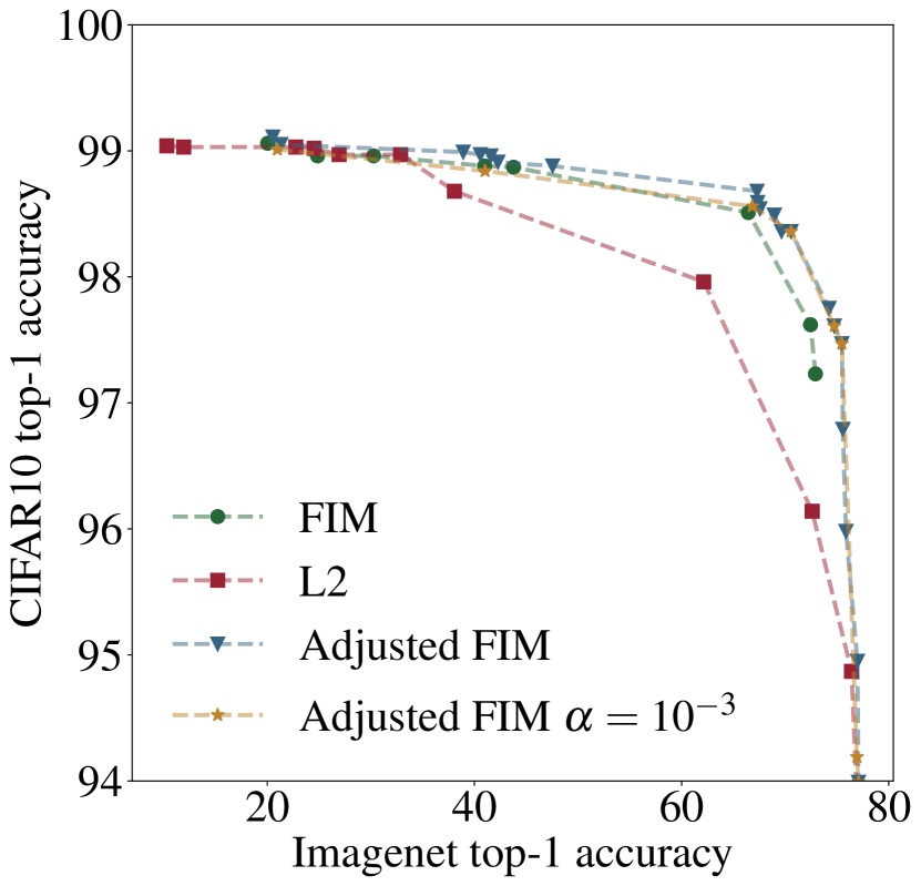
Figure 1: Pareto fronts of different regularization methods when fine-tuning a DINO ViT-B/16 pretrained on ImageNet to CIFAR10.

Hello

Figure 2: FIM value distributions on ViT-B/16

Hello Hello Hello Hello Hello Hello Hello Hello Hello Hello Hello Hello Hello Hello Hello Hello

We start by validating the expected properties of FIM by fine-tuning the pre-trained DINO ViT-B/16 ImageNet1k model on the CIFAR10 dataset. We vary the learning rate and the FIM regularization weight. After training, we evaluate the performance by computing: a) top-1 accuracy on the CIFAR10 dataset, and b) top-1 accuracy on ImageNet1k dataset. To evaluate the reverse transfer performance from CIFAR10 to ImageNet1k we attach the ImageNet1k classification head from the pre-trained model to the fine-tuned backbone.

Figure 2 shows the cross-task Pareto fronts for each fine-tuning method. We observe that as the regularization weight is increased, both methods improve in terms of their performance on ImageNet1k. However, since FIM regularizes parameters preferentially, its performance on CIFAR10 does not decrease in contrast to the naive $L_{2}$ regularization approach discussed in Section 2.

While the $L_{2}$ regularization approach manages to fully recover 77% top-1 accuracy on ImageNet1k this is not the case for FIM regularization, even for very high regularization weights $\lambda$, which saturates at around 73% (Figure 2).

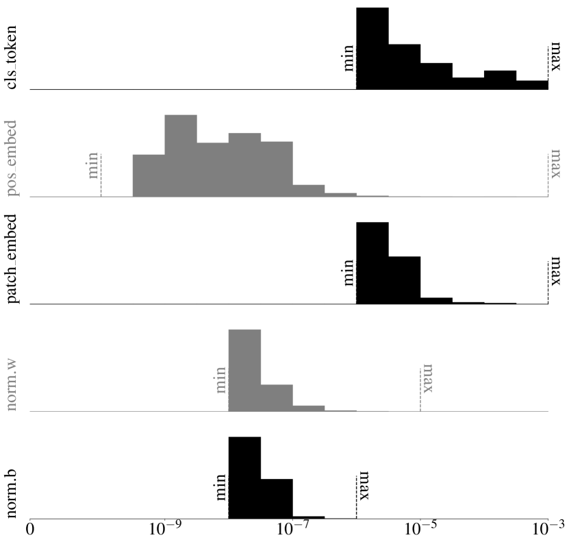
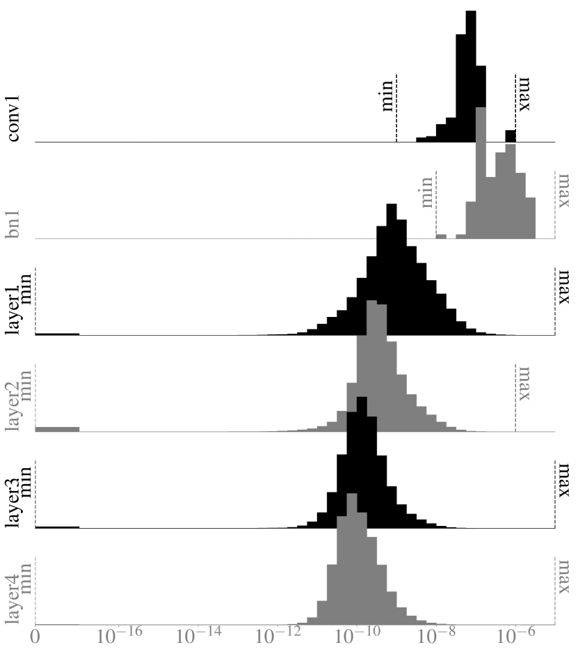
Figure 6: FIM distribution of the non-block layers of ViT-B/16.

Figure 7: FIM distribution of outermost layers of ResNet50. Note that while the values seem better behaved than in the case of ViT-B/16, all blocks still have some parameters with 0 FIM value.

We attribute this to the fact that a significant proportion of parameters in the ViT-B/16 have low values (see the distribution of FIM values in Figure 2 and refer to Appendix B for a more detailed breakdown). By decomposing the FIM into a layer-wise distributional plot (Figure 7) we observe that the first attention layer has a large proportion of very small values within the range of $10^{-30}$. In fact, some of the FIM values are 0, making $\|\cdot\|_{F}$ a pseudo-norm, i.e. minimizing $\|\cdot\|_{F}$ does not imply fully recovering all of the parameters. In other words, $F$ is poorly-conditioned, and parameters with small FIM values are allowed to vary freely making full recovery of the model impossible. To resolve this we rescale $F$:

$$F_{\alpha}=(1-\alpha)F+\alpha\bar{F},$$ (5)

where $\bar{F}$ is the mean of $F$ and $\alpha\in[0,1]$ is an additional hyperparameter. This rescaling pushes $\|\cdot\|_{F}$ closer to $\|\cdot\|_{2}$, which is not ill-conditioned. Adjusted FIM in Figure 2 sweeps the Pareto front with varying $\alpha$ whereas Adjusted FIM $\alpha=10^{-3}$ sweeps the Pareto front with a fixed $\alpha$ – both strategies for rectification produce a Pareto front that improves on $L_{2}$ and the unadjusted FIM regularization.

Robustness analysis

Table 1: Results of fine-tuning a pre-trained DINO model. We report results for our naive $L_{2}$ regularization method $\|\theta-\theta_{\text{SSL}}\|_{2}^{2}$, EWC FIM and the Adjusted FIM ($\alpha=10^{-3}$) regularized variants. We compare against a competitively tuned ERM baseline (Vapnik, 1995), finetuned from the same pre-trained DINO model – this differs from the pre-trained supervised initialization of Sagawa et al. (2019). For more details and hyperparameters see Appendix A. Given a validation set without group labels, we choose hyperparameters with the highest validation top-1 accuracy. Results are reported on the worst sub-group test split over 5 trials (mean $\pm$ 1-std).

	Finetuning method	Waterbirds	CelebA
		Test WGA	Test WGA
ViT-B/16	ERM	$70.53(\pm 2.07)$	$41.22(\pm 1.86)$
	FIM (ours)	$75.39(\pm 1.38)$	$43.22(\pm 1.49)$
	Adjusted FIM (ours)	$71.00(\pm 3.55)$	$43.88(\pm 2.52)$
	$L_{2}$ (ours)	$72.43(\pm 1.30)$	$38.89(\pm 1.62)$
ResNet50	ERM	$62.55(\pm 1.73)$	$40.55(\pm 1.47)$
	FIM (ours)	$60.90(\pm 0.54)$	$41.85(\pm 1.40)$
	Adjusted FIM (ours)	$60.29(\pm 1.63)$	$41.85(\pm 1.70)$
	$L_{2}$ (ours)	$39.84(\pm 2.26)$	$38.15(\pm 0.85)$

We use the proposed regularization to finetune DINO models on the biased Waterbirds (Sagawa et al., 2019) and CelebA (Liu et al., 2015) datasets. We fine-tune all of the mentioned methods with varying hyperparameters, extracted from a 20 trial random hyper-parameter sweep, evaluated over 5 replicates. We evaluate a simplified scenario where we assume we don’t have access to group information and pick the validation hyper-parameters that maximize the total top-1 accuracy. This parallels the ERM evaluation from Sagawa et al. (2019). We emphasize that most other methods for improving worst sub-group performance, such as Sagawa et al. (2019); Liu et al. (2021); Kirichenko et al. (2022), assume access to group labels in the validation set and therefore are not a suitable comparison.

We find that FIM based regularization techniques outperform standard finetuning in all but one scenario (ResNet50 on Waterbirds), demonstrating the utility of regularizing towards previously learned SSL representations. With ViT-B/16 we observe a 5% improvement on Waterbirds and 2% improvement on CelebA compared to our baseline ERM model. With ResNet50 this regularization improves upon ERM by approximately 1% on CelebA, but performs worse on the Waterbirds dataset.

4 Conclusion

In this work we present a novel treatment of SSL finetuning under the lens of a Bayesian continual learning framework. We empirically demonstrate that constraining the fine-tuned model posterior towards the original (label) bias free pre-trained model posterior improves performance for the worst sub groups in Celeb-A and Waterbirds. Future work will explore how other CL techniques could be leveraged to further improve SSL finetuning procedures.

5 Acknowledgements

The authors would like to thank the following people for their help throughout the process of writing this paper, in alphabetical order: Barry-John Theobald and Miguel Sarabia del Castillo. Additionally, we thank Li Li, Mubarak Seyed Ibrahim, Okan Akalin, and the wider Apple infrastructure team for assistance with developing scalable, fault tolerant code.

Appendix A Experiment details

Table 2: Hyperparameters for finetuning on CIFAR10

Hyperparameter	Finetuning method
	FIM	adjusted FIM	$L_{2}$
learning rate	$\{0.3,1,3\}\times 10^{-5}$	$\{1,3\}\times 10^{-5}$	$\{0.3,1,3\}\times 10^{-5}$
regularization weight	$0,10^{\{4,5,6,7,8,9,10\}}$	$10^{\{4,5,6,7,8,9\}}$	$0,10^{\{-4,-3,-2,-1,0,1,2\}}$
$\alpha$	—	$10^{\{-8,-7,-6,-4,-3,-2,-1\}}$	—
batch size	4032	4032	4032
epochs	120	120	120
warmup epochs	20	20	20
drop path rate	0	0	0
optimizer	adamw	adamw	adamw
learning rate schedule	cosine	cosine	cosine
learning rate scaling value	256	256	256
weight decay	0.3	0.3	0.3
weight decay end	0.7	0.7	0.7
augmentation	randaug	randaug	randaug
aug multiplicity	2	2	2

CIFAR10 experiments in Section 3 were run with hyperparameters in Table 2. Each hyperparameter combination was run once and its performance was evaluated at the end of training on CIFAR10 and Imagenet1k test sets. As mentioned before, to evaluate the performance of the fintuned backbone on Imagenet1k, we attached an Imagenet1k classifier head which was trained before the backbone was finetuned. Figure 2 was produced by computing the convex hull over the (CIFAR10 top-1 accuracy, Imagenet1k top-1 accuracy) data points for each group of runs.

Table 3: Hyperparameter sweep for finetuning ResNet50 on Waterbirds

Hyperparameter	Finetuning method
	FIM	adjusted FIM	$L_{2}$	ERM
learning rate	$10^{-2,-3,-4}$
regularization weight	$10^{\{5,6,7\}}$	$10^{\{5,6,7\}}$	$10^{\{-1,0,1\}}$	—
$\alpha$	—	$10^{-3}$	—	—
batch size	128, 256
epochs	120
warmup epochs	0
drop path rate	0
optimizer	SGD(momentum=0.9)
learning rate schedule	constant
learning rate scaling value	1.0
weight decay	$\{0,10^{-4},1.5\times 10^{-6}\}$
weight decay end	—
augmentation	imagenet, crop_scale=(0.2, 1.0)
aug multiplicity	1

Table 4: Hyperparameter sweep for finetuning ViT-B/16 on Waterbirds

Hyperparameter	Finetuning method
	FIM	adjusted FIM	$L_{2}$	ERM
learning rate	$10^{-6,-5,-4}$
regularization weight	$10^{\{5,6,7\}}$	$10^{\{5,6,7\}}$	$10^{\{-1,0,1\}}$	—
$\alpha$	—	$10^{-3}$	—	—
batch size	128, 256
epochs	120
warmup epochs	0
drop path rate	0
optimizer	AdamW($\beta_{1}=0.9,\beta_{2}=0.95$)
learning rate schedule	cosine
learning rate scaling value	1.0
weight decay	$\{0,10^{\{-3,-2,-1\}}\}$
weight decay end	—
augmentation	imagenet, crop_scale=(0.2, 1.0)
aug multiplicity	1

Waterbirds experiments in Section 3 were run with hyperparameters in Table 3 and Table 4. 18 combinations were randomly sampled without replacement and each sampled hyperparameter combination was run five times. We select the best performing validation hyper-parameter set for the top-1 metric (using no group labels) and use that to report the test worst sub-group accuracy for all methods.

Table 5: Hyperparameter sweep for finetuning ResNet50 on Celeb-A

Hyperparameter	Finetuning method
	FIM	adjusted FIM	$L_{2}$	ERM
learning rate	$10^{-2,-3,-4}$
regularization weight	$10^{\{5,6,7\}}$	$10^{\{5,6,7\}}$	$10^{\{-3,-2,-1\}}$	—
$\alpha$	—	$10^{-3}$	—	—
batch size	2048
epochs	300
warmup epochs	0
drop path rate	0
optimizer	LARS(momentum=0.9)
learning rate schedule	cosine
learning rate scaling value	256.0
weight decay	$\{0,10^{-4},1.5\times 10^{-6}\}$
weight decay end	—
augmentation	imagenet, crop_scale=(0.2, 1.0)
aug multiplicity	1

Table 6: Hyperparameter sweep for finetuning ViT-B/16 on Celeb-A

Hyperparameter	Finetuning method
	FIM	adjusted FIM	$L_{2}$	ERM
learning rate	$10^{-6,-5,-4}$
regularization weight	$10^{\{5,6,7\}}$	$10^{\{5,6,7\}}$	$10^{\{-1,0,1\}}$	—
$\alpha$	—	$10^{-3}$	—	—
batch size	2048, 4096
epochs	60
warmup epochs	0
drop path rate	0
optimizer	AdamW($\beta_{1}=0.9,\beta_{2}=0.95$)
learning rate schedule	cosine
learning rate scaling value	256.0
weight decay	$\{0,10^{\{-3,-2,-1\}}\}$
weight decay end	—
augmentation	imagenet, crop_scale=(0.2, 1.0)
aug multiplicity	1

Celeb-A experiments in Section 3 were run with hyperparameters in Table 5 and Table 6. 18 combinations were randomly sampled without replacement and each sampled hyperparameter combination was run five times. We select the best performing validation hyper-parameter set for the top-1 metric (using no group labels) and use that to report the test worst sub-group accuracy for all methods.

Appendix B FIM distributions

Figure 3: Overall FIM distribution of ViT-B/16

Figure 4: Overall FIM distribution of ResNet50

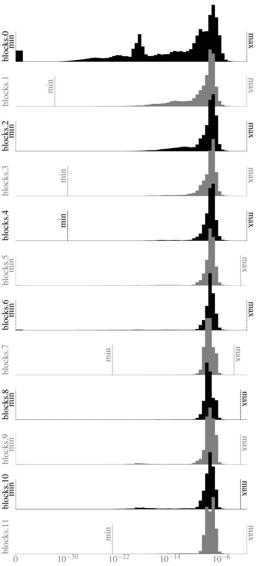
Figure 5: FIM distribution of outermost layers of ViT-B/16. Note that the earlier blocks have much wider spread of FIM values.

References

- Amari (1998) Shun-ichi Amari. Natural gradient works efficiently in learning. Neural Comput., 10(2):251–276, 1998. doi: 10.1162/089976698300017746. URL https://doi.org/10.1162/089976698300017746.
- Caron et al. (2021) Mathilde Caron, Hugo Touvron, Ishan Misra, Hervé Jégou, Julien Mairal, Piotr Bojanowski, and Armand Joulin. Emerging properties in self-supervised vision transformers. CoRR, abs/2104.14294, 2021. URL https://arxiv.org/abs/2104.14294.
- Chen et al. (2020a) Ting Chen, Simon Kornblith, Mohammad Norouzi, and Geoffrey E. Hinton. A simple framework for contrastive learning of visual representations. In Proceedings of the 37th International Conference on Machine Learning, ICML 2020, 13-18 July 2020, Virtual Event, volume 119 of Proceedings of Machine Learning Research, pp. 1597–1607. PMLR, 2020a. URL http://proceedings.mlr.press/v119/chen20j.html.
- Chen et al. (2020b) Ting Chen, Simon Kornblith, Kevin Swersky, Mohammad Norouzi, and Geoffrey E. Hinton. Big self-supervised models are strong semi-supervised learners. In Hugo Larochelle, Marc’Aurelio Ranzato, Raia Hadsell, Maria-Florina Balcan, and Hsuan-Tien Lin (eds.), Advances in Neural Information Processing Systems 33: Annual Conference on Neural Information Processing Systems 2020, NeurIPS 2020, December 6-12, 2020, virtual, 2020b. URL https://proceedings.neurips.cc/paper/2020/hash/fcbc95ccdd551da181207c0c1400c655-Abstract.html.
- Daxberger et al. (2021) Erik Daxberger, Agustinus Kristiadi, Alexander Immer, Runa Eschenhagen, Matthias Bauer, and Philipp Hennig. Laplace redux - effortless bayesian deep learning. In Marc’Aurelio Ranzato, Alina Beygelzimer, Yann N. Dauphin, Percy Liang, and Jennifer Wortman Vaughan (eds.), Advances in Neural Information Processing Systems 34: Annual Conference on Neural Information Processing Systems 2021, NeurIPS 2021, December 6-14, 2021, virtual, pp. 20089–20103, 2021. URL https://proceedings.neurips.cc/paper/2021/hash/a7c9585703d275249f30a088cebba0ad-Abstract.html.
- Deng et al. (2009) Jia Deng, Wei Dong, Richard Socher, Li-Jia Li, Kai Li, and Fei-Fei Li. Imagenet: A large-scale hierarchical image database. In 2009 IEEE Computer Society Conference on Computer Vision and Pattern Recognition (CVPR 2009), 20-25 June 2009, Miami, Florida, USA, pp. 248–255. IEEE Computer Society, 2009. doi: 10.1109/CVPR.2009.5206848. URL https://doi.org/10.1109/CVPR.2009.5206848.
- Dosovitskiy et al. (2021) Alexey Dosovitskiy, Lucas Beyer, Alexander Kolesnikov, Dirk Weissenborn, Xiaohua Zhai, Thomas Unterthiner, Mostafa Dehghani, Matthias Minderer, Georg Heigold, Sylvain Gelly, Jakob Uszkoreit, and Neil Houlsby. An image is worth 16x16 words: Transformers for image recognition at scale. In 9th International Conference on Learning Representations, ICLR 2021, Virtual Event, Austria, May 3-7, 2021. OpenReview.net, 2021. URL https://openreview.net/forum?id=YicbFdNTTy.
- Goyal et al. (2021) Priya Goyal, Mathilde Caron, Benjamin Lefaudeux, Min Xu, Pengchao Wang, Vivek Pai, Mannat Singh, Vitaliy Liptchinsky, Ishan Misra, Armand Joulin, and Piotr Bojanowski. Self-supervised pretraining of visual features in the wild. CoRR, abs/2103.01988, 2021. URL https://arxiv.org/abs/2103.01988.
- Grill et al. (2020) Jean-Bastien Grill, Florian Strub, Florent Altché, Corentin Tallec, Pierre H. Richemond, Elena Buchatskaya, Carl Doersch, Bernardo Ávila Pires, Zhaohan Guo, Mohammad Gheshlaghi Azar, Bilal Piot, Koray Kavukcuoglu, Rémi Munos, and Michal Valko. Bootstrap your own latent - A new approach to self-supervised learning. In Hugo Larochelle, Marc’Aurelio Ranzato, Raia Hadsell, Maria-Florina Balcan, and Hsuan-Tien Lin (eds.), Advances in Neural Information Processing Systems 33: Annual Conference on Neural Information Processing Systems 2020, NeurIPS 2020, December 6-12, 2020, virtual, 2020. URL https://proceedings.neurips.cc/paper/2020/hash/f3ada80d5c4ee70142b17b8192b2958e-Abstract.html.
- He et al. (2016) Kaiming He, Xiangyu Zhang, Shaoqing Ren, and Jian Sun. Deep residual learning for image recognition. In 2016 IEEE Conference on Computer Vision and Pattern Recognition, CVPR 2016, Las Vegas, NV, USA, June 27-30, 2016, pp. 770–778. IEEE Computer Society, 2016. doi: 10.1109/CVPR.2016.90. URL https://doi.org/10.1109/CVPR.2016.90.
- Kirichenko et al. (2022) Polina Kirichenko, Pavel Izmailov, and Andrew Gordon Wilson. Last layer re-training is sufficient for robustness to spurious correlations. CoRR, abs/2204.02937, 2022. doi: 10.48550/arXiv.2204.02937. URL https://doi.org/10.48550/arXiv.2204.02937.
- Kirkpatrick et al. (2017) James Kirkpatrick, Razvan Pascanu, Neil Rabinowitz, Joel Veness, Guillaume Desjardins, Andrei A Rusu, Kieran Milan, John Quan, Tiago Ramalho, Agnieszka Grabska-Barwinska, et al. Overcoming catastrophic forgetting in neural networks. Proceedings of the national academy of sciences, 114(13):3521–3526, 2017.
- Krizhevsky (2009) Alex Krizhevsky. Learning multiple layers of features from tiny images. Technical report, Canadian Institute for Advanced Research, 2009.
- Kunstner et al. (2019) Frederik Kunstner, Philipp Hennig, and Lukas Balles. Limitations of the empirical fisher approximation for natural gradient descent. In Hanna M. Wallach, Hugo Larochelle, Alina Beygelzimer, Florence d’Alché-Buc, Emily B. Fox, and Roman Garnett (eds.), Advances in Neural Information Processing Systems 32: Annual Conference on Neural Information Processing Systems 2019, NeurIPS 2019, December 8-14, 2019, Vancouver, BC, Canada, pp. 4158–4169, 2019. URL https://proceedings.neurips.cc/paper/2019/hash/46a558d97954d0692411c861cf78ef79-Abstract.html.
- Laplace (1986) PS Laplace. Mémoires de mathématique et de physique, tome sixieme [memoir on the probability of causes of events.]. Stat. Sci., pp. 366–367, 1986.
- Liu et al. (2021) Evan Zheran Liu, Behzad Haghgoo, Annie S. Chen, Aditi Raghunathan, Pang Wei Koh, Shiori Sagawa, Percy Liang, and Chelsea Finn. Just train twice: Improving group robustness without training group information. In Marina Meila and Tong Zhang (eds.), Proceedings of the 38th International Conference on Machine Learning, ICML 2021, 18-24 July 2021, Virtual Event, volume 139 of Proceedings of Machine Learning Research, pp. 6781–6792. PMLR, 2021. URL http://proceedings.mlr.press/v139/liu21f.html.
- Liu et al. (2015) Ziwei Liu, Ping Luo, Xiaogang Wang, and Xiaoou Tang. Deep learning face attributes in the wild. In 2015 IEEE International Conference on Computer Vision, ICCV 2015, Santiago, Chile, December 7-13, 2015, pp. 3730–3738. IEEE Computer Society, 2015. doi: 10.1109/ICCV.2015.425. URL https://doi.org/10.1109/ICCV.2015.425.
- Martens & Grosse (2015) James Martens and Roger B. Grosse. Optimizing neural networks with kronecker-factored approximate curvature. In Francis R. Bach and David M. Blei (eds.), Proceedings of the 32nd International Conference on Machine Learning, ICML 2015, Lille, France, 6-11 July 2015, volume 37 of JMLR Workshop and Conference Proceedings, pp. 2408–2417. JMLR.org, 2015. URL http://proceedings.mlr.press/v37/martens15.html.
- McCloskey & Cohen (1989) Michael McCloskey and Neal J Cohen. Catastrophic interference in connectionist networks: The sequential learning problem. In Psychology of learning and motivation, volume 24, pp. 109–165. Elsevier, 1989.
- Polyak & Juditsky (1992) Boris T Polyak and Anatoli B Juditsky. Acceleration of stochastic approximation by averaging. SIAM journal on control and optimization, 30(4):838–855, 1992.
- Sagawa et al. (2019) Shiori Sagawa, Pang Wei Koh, Tatsunori B. Hashimoto, and Percy Liang. Distributionally robust neural networks for group shifts: On the importance of regularization for worst-case generalization. CoRR, abs/1911.08731, 2019. URL http://arxiv.org/abs/1911.08731.
- Smola et al. (2003) Alexander J. Smola, Vishy Vishwanathan, and Eleazar Eskin. Laplace propagation. In Sebastian Thrun, Lawrence K. Saul, and Bernhard Schölkopf (eds.), Advances in Neural Information Processing Systems 16 [Neural Information Processing Systems, NIPS 2003, December 8-13, 2003, Vancouver and Whistler, British Columbia, Canada], pp. 441–448. MIT Press, 2003. URL https://proceedings.neurips.cc/paper/2003/hash/7fd804295ef7f6a2822bf4c61f9dc4a8-Abstract.html.
- Vapnik (1995) Vladimir Vapnik. The Nature of Statistical Learning Theory. Springer, 1995. ISBN 978-1-4757-2442-4. doi: 10.1007/978-1-4757-2440-0. URL https://doi.org/10.1007/978-1-4757-2440-0.