Effective-one-body waveforms for precessing coalescing compact binaries with post-newtonian twist

Abstract

Spin precession is a generic feature of compact binary coalescences, which leaves clear imprints in the gravitational waveforms. Building on previous work, we present an efficient time domain inspiral-merger-ringdown effective-one-body model (EOB) for precessing binary black holes, which incorporates subdominant modes beyond $\ell=2$, and the first EOB frequency domain approximant for precessing binary neutron stars. We validate our model against 99 “short” numerical relativity precessing waveforms, where we find median mismatches of $5\times 10^{-3}$, $7\times 10^{-3}$ at inclinations of $0$, $\pi/3$, and 21 “long” waveforms with median mismatches of $4\times 10^{-3}$ and $5\times 10^{-3}$ at the same inclinations. Further comparisons against the state-of-the-art NRSur7dq4 waveform model yield median mismatches of $4\times 10^{-3},1.8\times 10^{-2}$ at inclinations of $0,\pi/3$ for 5000 precessing configurations with the precession parameter $\chi_{p}$ up to 0.8 and mass ratios up to 4. To demonstrate the computational efficiency of our model we apply it to parameter estimation, and re-analyze the gravitational-wave events GW150914, GW190412, and GW170817.

I Introduction

From the very first direct detection of a coalescing binary black hole (BBH) system, gravitational wave astronomy has provided the scientific community with important (and at times unexpected) indications about black hole (BH) and neutron star (NS) physics Abbott et al. (2016a, 2019a, 2018). The LIGO-Virgo collaborations have detected (as of the first half of the third observing run) $\sim 50$ BBH systems Abbott et al. (2016b, 2017a, 2017b, 2017c, 2019b); Venumadhav et al. (2019, 2020); Nitz et al. (2019, 2020); Abbott et al. (2020a, b, c), two binary neutron star mergers (BNSs) Abbott et al. (2017d, 2020d), and two BHNS systems Abbott et al. (2021a) with a large number of significant triggers whose parameters have not been published yet. Analyses so far indicate that – out of the detected BBH events – two systems have at least one spinning BH component, and that for eleven binaries the effective spin-parameter $\chi_{\rm eff}$ [see Eq. (3)] is nonzero with more than $95\%$ credibility. Two events, GW190521 Abbott et al. (2020c, e) and GW190412 Abbott et al. (2020b), individually exhibit marginal evidence for the phenomenon of precession Abbott et al. (2021b, c), whereby the orbital plane and the black holes’ spins precess about the total angular momentum of the system. This affects the resulting gravitational waveforms by modulating the amplitude and contributing to the phase in a time-dependent manner Apostolatos et al. (1994). Wider population studies of all the currently observed signals further indicate evidence for nonvanishing spin-orbit misalignment among the population of merging BBH events, with the spin-precession parameter $\chi_{p}$ [see Eq. (4)] non-null at more than $99\%$ credibility.

Source properties are extracted from the data with matched filtering techniques that employ waveform templates, i.e., theoretical models of the gravitational waves (GWs) emitted by the two coalescing bodies. Waveform templates – also called approximants – should incorporate a large amount of physical information: the physics that can be extracted from the data is (at best) that which is contained within the model itself. Further, such approximants should also be faithful to numerical relativity (NR) simulations at high frequencies and computationally efficient, in order to be employed in parameter estimation (PE) which can require the generation of up to $\mathcal{O}(10^{5}-10^{6})$ waveforms.

The last decade has seen a flurry of activity in the development of various waveform approximants. Several different approximant “families” have now matured into their fourth generation versions that incorporate higher multipolar modes, spin precession, and robust fits to NR data for the merger-ringdown stages. These families are clearly distinguished by the underlying approaches that are employed to build the waveforms.

The Effective-One-Body (EOB) semi-analytic family of waveforms for BBH Buonanno and Damour (1999, 2000); Damour et al. (2000); Damour (2001); Buonanno et al. (2006); Damour et al. (2015) and BNS Damour and Nagar (2010); Damour et al. (2012); Bernuzzi et al. (2012) systems maps the general-relativistic two-body problem into the effective problem of describing the evolution of a test mass orbiting around a deformed Kerr metric. Such a system is entirely defined by a Hamiltonian, which describes the conservative motion, and a prescription for the dissipative dynamics, namely the waveform and radiation reaction. By relying on systematic resummation of Post-Netwonian (PN) results, EOB models are faithful also in the high-speed, strong-field regime. They can be extendend beyond the merger stage of the binary with information from NR simulations. Two main avatars of this family exist: the SEOBNR Bohé et al. (2017); Babak et al. (2017); Cotesta et al. (2018); Hinderer et al. (2016); Steinhoff et al. (2016); Lackey et al. (2019); Matas et al. (2020); Ossokine et al. (2020) and the TEOBResumS Damour and Nagar (2014a); Bernuzzi et al. (2015); Nagar et al. (2017, 2018); Akcay et al. (2019); Nagar et al. (2020) approximants. They differ from one another in choices of resummation within the conservative Hamiltonian, the amount of PN and NR information employed and the radiative sector. A detailed investigation of the differences between the two conservative Hamiltonians is presented in Ref. Rettegno et al. (2019). Both models include higher-order modes, tidal effects and precession (albeit TEOBResumS description of the latter previously being limited to the inspiral), with TEOBResumS also being able to generate waveforms along generic orbits Chiaramello and Nagar (2020); Nagar et al. (2021a); Albanesi et al. (2021); Nagar et al. (2021b); Nagar and Rettegno (2021).

The most commonly used approximant family in PE are the phenomenological models Ajith et al. (2007, 2008, 2011); Santamaria et al. (2010); Husa et al. (2016); Khan et al. (2016); Pratten et al. (2020); Estellés et al. (2021a, 2020, b); Hamilton et al. (2021) which combine PN waveforms with fits to hybrid EOB-NR waveforms to obtain computationally cheap, yet accurate, waveforms that can cover the binary evolution from the early inspiral regime (for which no NR simulation is available) up to merger. These models include higher-order modes London et al. (2018); García-Quirós et al. (2020); Khan et al. (2019a), precession Hannam et al. (2014); Schmidt et al. (2015); Khan et al. (2019b); Pratten et al. (2021) and tidal effects, which can be incorporated via time or frequency domain NRTidal models Dietrich et al. (2017, 2019).

Finally, NR surrogates Blackman et al. (2014, 2017); Varma et al. (2019a, b); Williams et al. (2019) directly interpolate large sets of NR simulations, and are able to provide fast and extremely accurate waveforms within their parameter space of validity.

In this paper we focus on the description of precessing compact binaries. We work within the EOB approach Buonanno and Damour (1999, 2000), and improve on the model TEOBResumS first presented in Ref. Akcay et al. (2021). In particular, we extend that precessing waveform model to (i) incorporate higher modes in the waveform for both BBHs and BNSs; (ii) incorporate the ringdown description for BBHs, to obtain a complete inspiral-merger-ringdown (IMR) approximant, (iii) provide an alternative, fast, frequency-domain approximant for BNS inspiral-merger and long BBH inspiral events based on the nonprecessing approach of Ref. Gamba et al. (2021b). TEOBResumS IMR precessing model for BBHs is validated by directly computing (mis)matches against a significant number of NR SXS SXS waveforms and against the waveform model $\tt{NRSur7dq4}$ Varma et al. (2019b). We additionally indirectly test its performance against the state-of -the-art $\tt{IMRPhenomXPHM}$ model Pratten et al. (2021), by comparing EOB/NR and Phenom/NR mismatches. Finally, we perform full PE to further compare the model to other existing approximants, and estimate the source parameters of the binary black hole merger events GW150914 Abbott et al. (2016a), GW190412 Abbott et al. (2020b), and the first binary neutron star inspiral-merger event GW170817 Abbott et al. (2017d).

This article is organized as follows: in Sec. II, we review our model and introduce the improvements we have made. Sec. III details the validation of our model against SXS and NRSur7dq4 waveforms. Sec. IV presents the results of our PE studies. We summarize our results and discuss future directions in Sec. V.

We work with geometrized units where $G=c=1$. $m_{1}$ and $m_{2}$ denote the masses of the primary and secondary components of the compact binary system. Accordingly, we define the mass ratio as $q\equiv m_{1}/m_{2}\geq 1$, the symmetric mass ratio $\nu=q/(1+q)^{2}$, the total mass as $M=m_{1}+m_{2}$ and the mass fraction $X_{i}$ as $X_{i}=m_{i}/M$ with $i=1,2$. As is standard,we employ mass-rescaled units within the EOB and the precession dynamics. However, when we make comparisons using interferometer sensitivity which varies with GW frequency $f$, thus with $M$, we restore the physical dimensions of $f$ and $M$, which we express in Hertz (Hz) and in solar masses ($M_{\odot}$), respectively. $\mathbf{S}_{1}$, $\mathbf{S}_{2}$ denote the dimensionful spin vectors of the binary components with their respective dimensionless spin parameters given by $\bm{\chi}_{i}=\mathbf{S}_{i}/m_{i}^{2}$ with $\chi_{i}\equiv|\bm{\chi}_{i}|$. The spin dependence in our baseline EOB model is expressed via the spin variables

$$\hat{\mathbf{S}}= M^{-2}(\mathbf{S}_{1}+\mathbf{S}_{2})=(X_{1}^{2}\bm{\chi}_{1}+X_{2}^{2}\bm{\chi}_{2})\,,$$ (1)

$$\hat{\mathbf{S}}_{*}= M^{-2}\Bigl{(}\frac{X_{2}}{X_{1}}\mathbf{S}_{1}+\frac{X_{1}}{X_{2}}\mathbf{S}_{2}\Bigr{)}=X_{1}X_{2}(\bm{\chi}_{1}+\bm{\chi}_{2})\,.$$ (2)

Let us also recall two standard definitions in the literature that pertain to the mass-weighted projections of the spins parallel and perpendicular to the Newtonian orbital angular momentum of the system $\mathbf{L}_{\text{N}}$. For $q\geq 1$, the parallel scalar is given by Ajith (2011); Damour (2001); Racine (2008)

$$\begin{split}\chi_{\text{eff}}\equiv&(X_{1}\bm{\chi}_{1}+X_{2}\bm{\chi}_{2})\cdot\!\hat{\,\mathbf{L}}_{\text{N}}\\ =&(\hat{\mathbf{S}}+\hat{\mathbf{S}}_{*})\cdot\!\hat{\,\mathbf{L}}_{\text{N}}\\ =&\,\tilde{a}_{0}\end{split}$$ (3)

where $\!\hat{\,\mathbf{L}}_{\text{N}}\equiv\mathbf{L}_{\text{N}}/|\mathbf{L}_{\text{N}}|$, and $\tilde{a}_{0}$ is one of the spin-parameters which often enter EOB models. This is a conserved quantity of the orbit-averaged precession equations over the precession timescale Racine (2008). The perpendicular scalar, first introduced in Ref. Schmidt et al. (2015), is defined as

$$\chi_{p}\equiv{m_{1}^{-2}}\max\left\{|\mathbf{S}_{1,\perp}|,q\frac{4+3q}{3+4q}|\mathbf{S}_{2,\perp}|\right\},$$ (4)

where $\mathbf{S}_{i,\perp}\equiv\mathbf{S}_{i}-(\!\hat{\,\mathbf{L}}_{\text{N}}\cdot\mathbf{S}_{i})\!\hat{\,\mathbf{L}}_{\text{N}}$ are the components of $\mathbf{S}_{i}$ perpendicular to $\!\hat{\,\mathbf{L}}_{\text{N}}$ for $i=1,2$.

II Method

In this section we describe in some detail the technical improvements that have been implemented in the model with respect to its first version in Ref. Akcay et al. (2021). After succintly recalling the conventions that we employ and describing the spin-aligned baseline model, we will highlight the main advancements introduced, which pertain to the coupling of the spin-evolution equations to the EOB orbital dynamics, the extension of the waveform to merger-ringdown, and the inclusion of higher ($\ell>2$) modes.

II.1 Reference frames and co-precessing waveform model

When the spins of the binary components $\mathbf{S}_{1},\mathbf{S}_{2}$ are not aligned with the orbital angular momentum $\mathbf{L}$ of the system, all three vectors precess around the total angular momentum vector $\mathbf{J}=\mathbf{L}+\mathbf{S}_{1}+\mathbf{S}_{2}$ Apostolatos et al. (1994). Accordingly, the orbital plane of the binary is not fixed throughout its evolution, but rather precesses, inducing non-trivial modulations in the gravitational waves detected by an inertial observer. In this scenario, the dominant emission of gravitational radiation happens along the direction perpendicular to the orbital plane, i.e., along the Newtonian orbital angular momentum $\mathbf{L}_{\text{N}}$ Schmidt et al. (2011, 2012); Boyle et al. (2011); O’Shaughnessy et al. (2011). It is then possible to identify a special “co-precessing” non-inertial frame, which follows the evolution of $\mathbf{L}_{\text{N}}$. In this frame, the modulations of amplitude and phase due to precession effectively disappear and the waveform can be well approximated by that emitted from an aligned spin system. Then, given the evolution of the co-precessing frame (i.e., of the vectors $\mathbf{S}_{1},\mathbf{S}_{2}$ and $\mathbf{L}_{\text{N}}$) and a co-precessing waveform, it is possible to rotate the latter into the inertial source frame and obtain the associated precessing waveform Schmidt et al. (2011, 2012). This technique is usually referred to as the “twist”, due to the time-dependent rotation which relates the two frames.

To perform the twist, one can in principle use either the frame set by the Newtonian orbital angular momentum $\mathbf{L}_{\text{N}}$ or $\mathbf{L}$. Since, by definition, $\mathbf{L}_{\text{N}}$ remains orthogonal to the orbital plane, we employ this frame for the twist. Ref. Pan et al. (2014a) has shown that the differences in the $\mathbf{L}$-frame vs. $\mathbf{L}_{\text{N}}$-frame twisted waveforms as compared with precessing NR waveforms are marginal. Accordingly, we define our inertial source frame such that its $z$ axis is aligned with the initial Newtonian orbital angular momentum $\mathbf{L}_{\text{N}}(0)$. Then, following usual conventions, we choose the line of sight vector $\hat{\bm{N}}$ to have spherical angles $(\iota,\pi/2-\phi_{\rm ref})$ and define the initial spin components, $\mathbf{S}_{1}(0),\mathbf{S}_{2}(0)$, in this so-called $L_{0}$ frame. We then track the evolution of $\mathbf{L}_{\text{N}}$ with respect to this frame via its spherical angles $\alpha$ and $\beta$, defined using the Cartesian components of the unit vector $\!\hat{\,\mathbf{L}}_{\text{N}}$

$$\alpha= \arctan(\!\hat{\,\mathbf{L}}_{\text{N}}{}_{y}/\!\hat{\,\mathbf{L}}_{\text{N}}{}_{x}),$$ (5)

$$\beta= \arccos(\!\hat{\,\mathbf{L}}_{\text{N}}{}_{z}).$$ (6)

A third angle $\gamma$, which identifies the co-precessing frame univocally with respect to the $L_{0}$ frame Boyle et al. (2011), is given by

$$\dot{\gamma}=\dot{\alpha}\cos\beta,$$ (7)

where the overdot denotes differentiation with respect to time. With $\alpha,\beta$, and $\gamma$, the twisted (precessing) multipolar waveform $h^{T}_{\ell m}$ is obtained via an Euler rotation

$$h^{T}_{\ell m}=\sum_{m^{\prime}=-m}^{m}h^{A}_{\ell m^{\prime}}D^{(\ell)}_{m^{\prime},m}(-\gamma,-\beta,-\alpha),$$ (8)

where $h^{A}_{\ell m}$ are the spin-aligned waveforms in the co-precessing frame and $D^{(\ell)}_{m^{\prime},m}(-\gamma,-\beta,-\alpha)$ are the Wigner D matrices, defined as

$$D^{(\ell)}_{m^{\prime},m}(\alpha,\beta,\gamma)=e^{-im^{\prime}\alpha}e^{-im\gamma}d^{\ell}_{m^{\prime},m}(\beta)$$ (9)

with

$$d^{\ell}_{m^{\prime},m}(\beta)= \sum_{k_{i}}^{k_{f}}(-1)^{k-m+m^{\prime}}$$

$$\times \frac{\sqrt{(\ell+m)!(\ell-m)!(\ell+m^{\prime})!(\ell-m^{\prime})!}}{k!(\ell+m-k)!(\ell-k-m^{\prime})!(k-m+m^{\prime})!}$$

$$\times \Bigl{[}\cos\frac{\beta}{2}\Bigr{]}^{2\ell-2k+m-m^{\prime}}\Bigl{[}\sin\frac{\beta}{2}\Bigr{]}^{2k-m+m^{\prime}}.$$

Finally, the plus and cross GW polarizations $h_{+}$ and $h_{\times}$ are obtained from the twisted modes as

$$h_{+}-ih_{\times}=\sum_{\ell,m}h^{T}_{\ell m}\,{}_{-2}Y^{\ell m}(\iota,\pi/2-\phi_{\rm ref})\,,$$ (10)

where ${}_{-2}Y^{\ell m}(\iota,\phi)$ are the standard spin weight $s=-2$ spherical harmonics.

Our baseline model for the spin-aligned co-precessing waveforms is TEOBResumS v2 Nagar et al. (2019a, 2020), a multipolar EOB model for quasi-circular BBH and BNS coalescences. Its non-spinning orbital sector contains analytical PN information suitably resummed via Padé approximants in both the Hamiltonian $H_{\rm EOB}$ and radiation reaction $\mathcal{F}_{\varphi}$. It is informed by NR via an effective parameter entering the EOB circular-orbit potential, $A$, at the relative 5PN order, $a_{6}$. Spin-orbit and spin-spin effects are included within the model Hamiltonian via the centrifugal radius $r_{c}$ Damour and Nagar (2014b) (or its inverse $u_{c}=r_{c}^{-1}$) and the gyro-gravitomagnetic coefficients $G_{S}$ and $G_{S*}$ Damour and Nagar (2014b) given in the DJS gauge Damour et al. (2008), and heceforth considered ar next-to-next-to-leading order (NNLO) Nagar et al. (2018). The EOB dynamics further contains a spin-orbit parameter, $c_{3}$, that is tuned to NR. Multipolar waveforms up to $\ell=m=5$ additionally contain spin-dependent terms, which are factorized and analytically resummed to improve their robustness in the strong-field regime Nagar et al. (2020). Tidal effects are included in both the multipolar waveform and the EOB conservative dynamics Nagar et al. (2018, 2019b); Akcay et al. (2019). The tidal sector of TEOBResumS contains contributions from the multipolar $\ell=2,3,4$ gravitoelectric and $\ell=2$ gravitomagnetic tidal coefficients, and the former are resummed via a gravitational self-force inspired expression Bini et al. (2012); Bini and Damour (2014); Akcay et al. (2019). The equation of state-dependent quadrupole-monopole terms are included at NNLO via $r_{c}$ Nagar (2011); Nagar et al. (2019b).

II.2 Spin dynamics

II.2.1 Time evolution of the orbital frequency

To obtain the time and frequency evolution of the Euler angles $\alpha,\beta$ and $\gamma$ we follow Ref. Akcay et al. (2021) and solve the PN spin-evolution equations for $\mathbf{S}_{1},\mathbf{S}_{2}$, and $\!\hat{\,\mathbf{L}}_{\text{N}}$ at the next-to-next-to-next-to-next to leading order (N4LO). To avoid clutter, we present the evolution equations up to the next-to-leading order, which can be cast into classical precession equations

$$\dot{\mathbf{S}}_{i} =\bm{\Omega}_{i}\times\mathbf{S}{}_{i},$$ (11a)

$$\dot{\hat{\,\mathbf{L}}}_{\text{N}} =\bm{\Omega}_{\text{NLO}}\times\!\hat{\,\mathbf{L}}_{\text{N}},$$ (11b)

for $i=1,2$. The precession frequencies are given by

$$\begin{split}\bm{\Omega}_{1}=&v^{5}\Bigl{[}\nu\left(2+\frac{3}{2}\frac{X_{2}}{X_{1}}\right)\!\hat{\,\mathbf{L}}_{\text{N}}+\frac{v}{2}\Bigl{\{}\mathbf{S}_{2}\\ &-3\Bigl{[}\Bigl{(}\frac{X_{2}}{X_{1}}\mathbf{S}_{1}+\mathbf{S}_{2}\Bigr{)}\cdot\!\hat{\,\mathbf{L}}_{\text{N}}\Bigr{]}\!\hat{\,\mathbf{L}}_{\text{N}}\Bigr{\}}\Bigr{]}\,,\end{split}$$ (12a)

$$\bm{\Omega}_{\text{NLO}}= -\frac{v}{\nu}\left(\bm{\Omega}_{1}+\bm{\Omega}_{2}\right),$$ (12b)

where $v$ is the relative speed of the binary components and $\bm{\Omega}_{2}$ is obtained from $\bm{\Omega}_{1}$ with $1\leftrightarrow 2$. The N$4$LO expression for this system of nine coupled ODEs is explicitly given in equations (4a)-(4b) and (7) of Ref. Akcay et al. (2021), together with an expression for the evolution of the orbital frequency under radiation reaction for which we employed a TaylorT4-resummed PN expression in our previous work: $\dot{\omega}^{\rm PN}$ Buonanno et al. (2003, 2009). Specifically, we employed the expressions from Ref. Chatziioannou et al. (2013) up to 3.5PN, which are integrated together with the spin ODEs in order to evolve the system under radiation reaction. Here we study three alternative reformulations for $\dot{\omega}$.

First, we consider a hybrid PN-EOB expression denoted by $\dot{\omega}^{\rm HY1}$. To obtain it, we begin by calculating the magnitude of the PN-corrected orbital angular momentum $L^{\text{PN}}(\omega)$ up to relative 4PN order (see App. G of Ref. Pratten et al. (2021)) and the orbital separation $r^{\text{PN}}(L^{\text{PN}})$ up to 4PN [Eqs. (12), (17), (18) of Ref. Nagar et al. (2019b)]. The resulting quantities are then employed to evaluate the EOB radiation reaction $\mathcal{F}_{\varphi}\equiv dL/dt$ along circular orbits for which the EOB radial momentum $p_{r*}$ is set to zero. The expression for $\dot{\omega}^{\rm HY1}$ is thus obtained as

$$\dot{\omega}^{\rm HY1}=\frac{\mathcal{F}_{\varphi}(r^{\text{PN}},L^{\text{PN}})}{dL^{\text{PN}}/d\omega}\,.$$ (13)

Alternatively, we can compute another hybrid PN-EOB expression, denoted by $\dot{\omega}^{\rm HY2}$, where we obtain $r(\omega)$ by numerically inverting the Hamilton equation for $\omega$, evaluated at $p_{r*}=0$:

$$\omega=\frac{\partial H_{\rm EOB}}{\partial p_{\varphi}}=\frac{1}{\nu H_{\rm EOB}H_{\rm eff}^{\rm orb}}\Bigl{[}Ap_{\varphi}u_{c}^{2}+H_{\rm eff}^{\rm orb}(G_{S}\hat{S}+G_{S_{*}}\hat{S}_{*})\Bigr{]}\,,$$ (14)

where $H_{\rm eff}^{\rm orb}$ is the orbital effective EOB hamiltionian. The magnitude of the orbital angular momentum $L(r)$ is then computed as the EOB circular-orbit angular momentum by analytically solving the equation

$$\partial_{r}H_{\rm EOB}=0\,.\\$$ (15)

Once $r(\omega)$ and $L(r)$ are known, we can compute $dL/d\omega=(dL/dr)(d\omega/dr)^{-1}$. The first piece, $(dL/dr)$, can be immediately obtained by differentiating the analytical solution found above; the second piece, $(d\omega/dr)$, is computed from Eq. (14). Then, we obtain $\dot{\omega}^{\rm HY2}$ as in Eq. (13).

Finally, we also consider “aligned” $\omega(t)$ relation as given by the integrating the EOB dynamics before computing the evolution of the spins. In this case, instead of solving an ODE system of 9 + 1 equations, we compute the cubic spline of $\omega(t)$ and use it to drive the spins evolution. Notably, the time axis of the EOB dynamics may in principle have a different origin with respect to the time axis of the spin dynamics, for which $t=0$ always corresponds to the reference (initial) frequency $\omega_{\rm ref}$ at which the spin components are specified. Therefore, by solving $\omega(t_{\rm EOB})=\omega_{\rm ref}$ for $t_{\rm EOB}$ we compute the timeshift $\Delta t=t_{\rm EOB}$ necessary to align the two time axes. Then, the frequency at each timestep of the spin dynamics is simply given by $\omega_{i}=\omega(t_{i}+\Delta t)$.

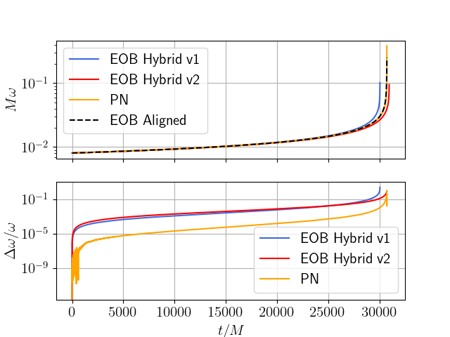
Figure 1: Example plot of the frequency evolution $\omega(t)$ of the spin dynamics, obtained by integrating pure PN (orange) or hybrid PN-EOB (blue and red) $\dot{\omega}(\omega)$ ODEs, or by employing the $\omega(t)$ relation as given by the aligned-spin EOB Hamilton equations (dubbed as “EOB aligned”, black dashed inline). The bottom panel displays the relative difference of the hybrid and PN methods with respect to the EOB aligned method. For the system considered, $\omega(t)^{\rm PN}$ remains the closest to the EOB frequency evolution at all times.

Figure 1 shows the different $\omega(t)$ relations obtained with the four methods described above for a system with $(q,\chi_{\rm eff},\chi_{\rm p})=(1.56,-0.06,0.28)$ at a reference frequency of $M\omega=0.0025$. The pure PN implementation $\omega^{\rm PN}$ is the closest to the EOB “aligned” $\omega$ evolution. The hybrid PN-EOB evolutions, instead, appear to either overestimate ($\rm HY1$) or underestimate ($\rm HY2$) dissipation effects by GW emission. Further, the hybrid evolution stops at lower values of $M\omega$ than the PN or “aligned EOB” one, because of the denominator of Eq. 13 becoming zero. The difference between the two hybrid versions can be qualitatively understood by considering a simple spinless, equal mass case. During the inspiral ($M\omega<0.06$), at a fixed $M\omega$ value $L^{\rm HY1}\geq L^{\rm HY2}$ and $|dL/d\omega|^{\rm HY1}\leq|dL/d\omega|^{\rm HY2}$. Therefore, by applying Eq. (13), the first hybrid version will emit GWs faster – and thus, have a steeper orbital frequency evolution – than the second hybrid, whose phase in turn will evolve slower than the “aligned” EOB one due to the (strong) assumption that the coalescence is along circular orbits and $p_{r*}=0$. Although all options are available in the publicly released TEOBResumS code, we find that the fully PN expression for $\dot{\omega}$ consistently gives the better performance in terms of accuracy and speed when computing mismatches against NR waveforms (see Sec. III). Therefore, all results obtained in this paper are obtained with $\dot{\omega}=\dot{\omega}^{\rm PN}$. We leave to future work the exploration of different purely PN formulations of $\dot{\omega}$.

II.2.2 Backward in time integration and $\alpha$ initial conditions

We further discuss two technical points: the initial condition for the Euler angle $\alpha$ and the behavior of the Euler angles when integrating backward in time. Neither is discussed in depth in the literature, as the former has no real implication on waveforms (since the in plane spin components are determined only up to a rotation, the single $x-y$ projections can vary: this is equivalent to choosing different $\alpha(0)$ initial conditions) and the latter stems from our hybrid PN-EOB implementation of the dynamics.

Regarding the first point, in our source frame, the initial conditions at $t=t_{0}$ (set to 0 without loss of generality) for the spin components and the angular momentum are straightforward to obtain. However, since $\!\hat{\,\mathbf{L}}_{\text{N}}(0)$ is parallel to the $z$ axis at $t=0$, $\alpha(t)$ is apparently undefined at $t=0$. Nonetheless, an expression for $\alpha(0)$ can be obtained using the direction of the initial “torque” at $t=0$ which only has $x,y$ components given by $\dot{\hat{\,\mathbf{L}}}_{\text{N}}{}_{x}(0),\dot{\hat{\,\mathbf{L}}}_{\text{N}}{}_{y}(0)$ yielding

$$\alpha(0)=\arctan\left(\frac{\dot{\hat{\,\mathbf{L}}}_{\text{N}}{}_{y}(0)}{\dot{\hat{\,\mathbf{L}}}_{\text{N}}{}_{x}(0)}\right).$$ (16)

Explicit expressions, as well as a comparison between $\alpha$ obtained at different PN orders, can be found in App. A. As far as we can tell, this is the only physically motivated initial condition for $\alpha(0)$ and although for simple precession $\alpha(0)$ is often in the fourth quadrant of the $x$-$y$ plane, it only equals the commonly-used $-\pi/2$ for special cases. On the other hand, there does not seem to be a physically motivated initial condition for the third Euler angle $\gamma$ defined by $\dot{\gamma}=\dot{\alpha}\cos\beta$. Therefore, one has the freedom to set $\gamma(0)=0$ or $\pm\pi/2$ or even $\alpha(0)$.

As for the second point, we observe that since the spin evolution is solved independently from the EOB dynamics, it may happen that for some binaries the initial orbital EOB frequency $\omega_{0}^{\text{EOB}}$ is smaller than the initial spin-evolution frequency $\omega_{0}^{S}$ specified by the user via $\omega_{0}^{S}=\pi f_{0}^{\rm Hz}M$, where $f_{0}^{\rm Hz}$ is input initial GW frequency in Hertz. Then, in order to twist the entire EOB waveform, it is necessary to integrate the spin dynamics backwards in time, at least to below $\omega_{0}^{\text{EOB}}$. Since all the directly evolved quantities vary continuously when going from $t>0$ to $t<0$, this procedure may appear straightforward at a first glance. However, as can be seen from Fig. 2, $\alpha(t)$ can exhibit a jump by $\pi$ due to the sign-change of both $\!\hat{\,\mathbf{L}}_{\text{N}}{}_{x}$ and $\!\hat{\,\mathbf{L}}_{\text{N}}{}_{y}$ when $\!\hat{\,\mathbf{L}}_{\text{N}}$ passes through the origin at $t=0$. Since a number of numerical interpolations of $\alpha(t),\beta(t)$ are required to compute the twist, when integrating backwards we compute

$$\alpha^{\prime}_{t<0}= \arctan(\!\hat{\,\mathbf{L}}_{\text{N}}{}_{y}/\!\hat{\,\mathbf{L}}_{\text{N}}{}_{x})+\pi,\,$$ (17)

$$\beta^{\prime}_{t<0}= -\arccos(\!\hat{\,\mathbf{L}}_{\text{N}}{}_{z}).$$ (18)

Note that this is analogous to changing into a different but equivalent source frame, in which $\beta\rightarrow-\beta$, $\alpha\rightarrow\alpha+\pi$ and $\!\hat{\,\mathbf{L}}_{\text{N}}=(\!\hat{\,\mathbf{L}}_{\text{N}}{}_{x},\!\hat{\,\mathbf{L}}_{\text{N}}{}_{y},\!\hat{\,\mathbf{L}}_{\text{N}}{}_{z})$ is mapped into itself. After removing the kinks this way then interpolating, we restore the original frame via $\alpha_{t<0}=\alpha^{\prime}_{t<0}-\pi$, $\beta_{t<0}=-\beta^{\prime}_{t<0}$, then perform the standard waveform twist.

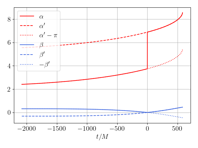
Figure 2: Backward time evolution of the Euler angles of Eqs. (5), (6). At $t=0$, $\alpha$ (straight red line) shows a jump of $\pi$, while $\beta$ (straight blue line) has a cusp. To correct this behavior and avoid interpolation issues, we compute $\alpha^{\prime}$ and $\beta^{\prime}$, which are then corrected to their true values after interpolation.

II.3 Coupling of the PN spin evolution to the EOB dynamics

When analyzing long signals, neglecting the evolution of the spins in the aligned-spin dynamics can lead to non-negligible errors. In principle, one should evolve the full EOB equations, coming from a genereral Hamiltonian where the orbital plane is not fixed. Similarly, the waveform and radiation reaction of the model, too, would need to be extended to incorporate the effect of the planar components of the spins. This general approach would increase the already significant computational cost related to the solution of the Hamilton equations. Luckily, it was found Pan et al. (2014b) that good agreement with NR waveforms can be achieved by simply replacing in the waveform and radiation reaction the fixed values of $\chi_{i}$ with the time-dependent projections of the spin vectors onto the orbital angular momentum, i.e., $\!\hat{\,\mathbf{L}}_{\text{N}}(t)\cdot\bm{\chi}_{i}(t)$.

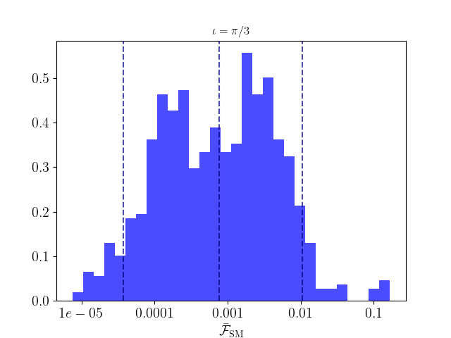
Figure 3: Comparison between waveforms obtained with and without projected spin dynamics for systems with the same intrinsic parameters as those examined in Sec. III.2 (see also App. B). For waveforms with large in-plane spin components, the effect of the spin projection is non-negligible and can lead to mismatches larger than $1\%$.

In our model, we (optionally) employ the spin dynamics to compute the projections of the spins onto $\!\hat{\,\mathbf{L}}_{\text{N}}$ either in the time or frequency domain. We proceed as follows: (i) the PN spin-dynamics is independently evolved with the N4LO description of the precession equations with $\dot{\omega}^{\text{PN}}$ detailed above; (ii) we interpolate the spin and angular momentum components as functions of the “spin” orbital frequency $\omega^{S}$; (iii) at each step of the EOB evolution, we compute the EOB orbital frequency and evaluate $\bm{\chi}_{i,z}(\omega_{\text{EOB}})\equiv\!\hat{\,\mathbf{L}}_{\text{N}}(\omega_{\text{EOB}})\cdot\bm{\chi}_{i}(\omega_{\text{EOB}})$ via the splines calculated above; (iv) finally, these quantities are inserted into the appropriate places in the EOB dynamics. This generic procedure is applied both when numerically evolving the ODE system and when applying the postadiabatic approximation (PA) of Ref. Nagar and Rettegno (2019).

Figure 3 displays the mismatches (see Sec. III.1) obtained between TEOBResumS waveforms with an inclination of $\iota=\pi/3$, evolved either with or without spin projection, for a set of waveforms with $q\in[1,6]$, $M\in[50,225]M_{\odot}$, $\chi_{\rm p}\in[0.,0.8]$ and $\chi_{\rm eff}\in[-0.45,0.65]$. Notably, although a large portion of the mismatches lie below the $10^{-3}$ threshold, the effect of the spin projection can be relevant for binaries with large in-plane spin components, i.e., $|\mathbf{S}_{i\perp}|$, for which the parallel components of the spins to the orbital angular momentum varies more.

II.4 BBH Merger-Ringdown

To model the final state of the BBH one can employ the fits of Ref. Jiménez-Forteza et al. (2017) with minor modifications to account for the non-null planar components of the BHs’ spins. Following Ref. Pratten et al. (2020), we define the remnant spin as:

$$\chi_{f}=\sqrt{(\chi_{f||})^{2}+(S_{\perp}/M_{f})^{2}},$$ (19)

where $\chi_{f||}$ and $M_{f}$ are estimated from the fits of Ref. Jiménez-Forteza et al. (2017) using the parallel component of the spins to the orbital angular momentum at merger, and $\mathbf{S}_{\perp}$ is given by

$$\mathbf{S}_{\perp}=\mathbf{S}_{1}(\omega_{\rm mrg})-\mathbf{S}_{1||}(\omega_{\rm mrg})+(1\leftrightarrow 2)\,.$$ (20)

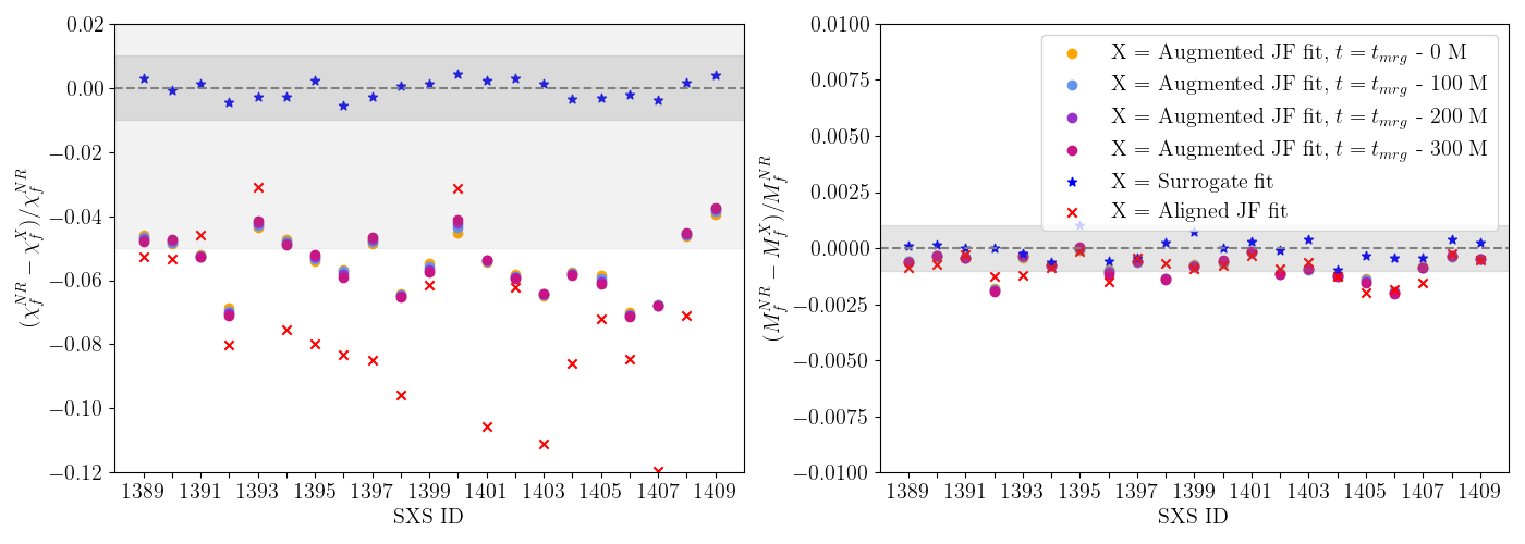
Figure 4: Relative differences in the dimensionless spin $\chi_{f}$ of the final black hole (left) and its mass $M_{f}$ (right) between NR simulations and fits of Ref. Varma et al. (2019b) (blue stars) and the various Jimenez-Forteza (JF) fits of Ref. Jiménez-Forteza et al. (2017). The latter are evaluated with the initial $z$ component spins (red crosses) or corrected to account for the precession by employing the spins at a reference time before merger like in Eq. (19). While the remnant mass is always estimated at the order of $10^{-3}$ and the two methods give comparable results, the surrogate fit for the remnant spin is up to an order of magnitude more precise. In the left panel, light (dark) gray bands highligt the $5\%$ ($1\%$) relative error interval; in the right panel the $1$‰  one.

Figure 4 displays the accuracy of the fits when compared to a handful of $\tt SXS$ NR simulations. We also compare the output of the fit above to the values obtained with the “simple” aligned-spin fit, and with the fits provided by the surrogate model of Refs. Varma et al. (2019c, b). Notably, while the mass of the remnant is approximated (by all approaches) at the level of $10^{-3}$, the difference $|\chi_{f}^{\rm NR}-\chi_{f}^{\rm surr}|$ is up to ten times smaller with respect to the other approaches. This result is not surprising, and is in line with the discussion presented in Ref. Varma et al. (2019b). Therefore, although all the results presented in this paper will employ Eq. (19), we also implemented the option to take $\chi_{f}$ and $M_{f}$ as input parameters. This way, by externally computing the remnant properties with the surrogate model (using the surfinBH package), we can easily obtain a precise description of the final BH.

For a complete model of the ringdown phase, it is necessary to also extend the Euler angles $\alpha,\beta,\gamma$ beyond the merger. The precession of the orbital momentum effectively stops at the merger, and the direction of the spin of the final black hole can be thought of as constant, and well-enough approximated by the direction of the angular momentum at merger. Therefore, one option is to simply prolong the angles by fixing them to their value at merger. Alternatively, it was observed that the evolution of the $\alpha$ angle can be approximately described through the difference of the $\ell=2$ fundamental quasinormal modes (QNMs) O’Shaughnessy et al. (2013); Ossokine et al. (2020)

$$\alpha(t)=\begin{cases}\alpha(t_{\rm mrg})+(\omega_{22}-\omega_{21})(t-t_{\rm mrg}),&\bm{\chi}_{f}\cdot\!\hat{\,\mathbf{L}}_{\text{N}}{}_{f}>0,\\ \alpha(t_{\rm mrg})+(\omega_{2-1}-\omega_{2-2})(t-t_{\rm mrg}),&\bm{\chi}_{f}\cdot\!\hat{\,\mathbf{L}}_{\text{N}}{}_{f}<0,\end{cases}$$ (21)

where $\bm{\chi}_{f}=\bm{\chi}_{1}(\omega_{\text{mrg}})+\bm{\chi}_{2}(\omega_{\text{mrg}})$ and $\omega_{\ell m}$ are the fundamental quasinormal-modes $\omega_{\ell m0}$ for $\ell=2$ and $m=2,1,-1,-2$ Berti et al. (2006). One can then fix $\beta$ to its value at the merger. $\gamma$ is subsequently computed by integrating its evolution equation (7). Both options for the post-merger evolution of $\alpha$ are curently available in TEOBResumS public code, and users can choose between one or the other. The default behavior is given by the quasinormal-modes extension, which gives marginally better results when computing mismatches between EOB and NR waveforms (see Sec. III).

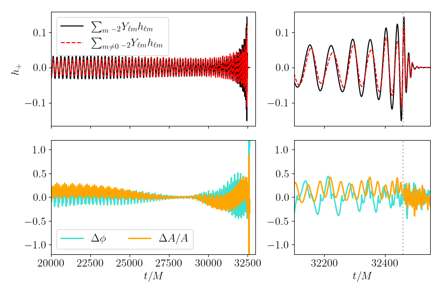
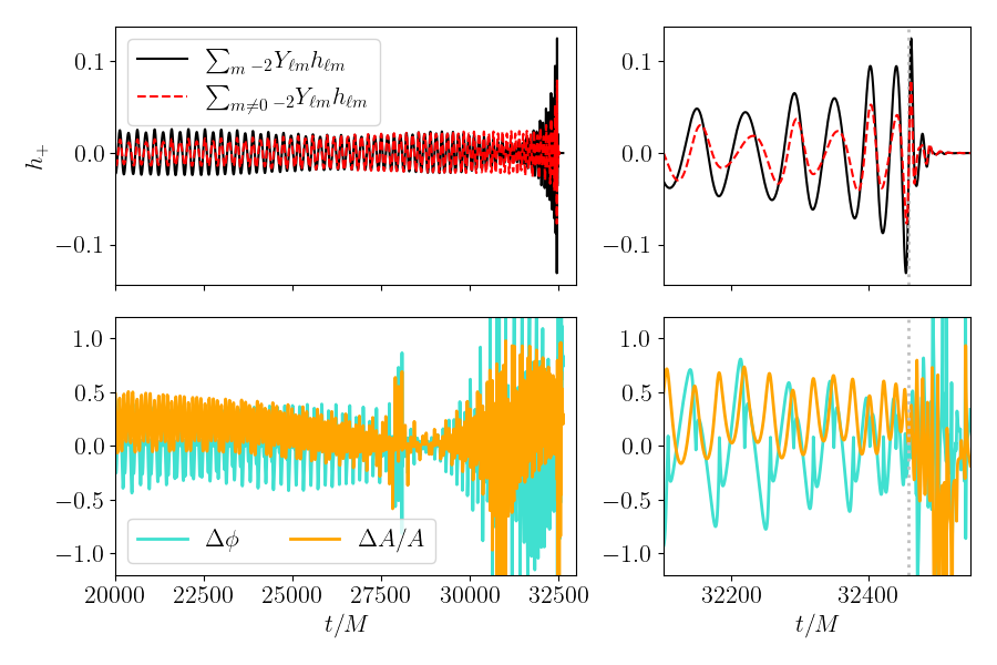
Figure 5: Plus polarization $h_{+}$ of the NR simulation $\tt{SXS:BBH:1409}$ having $(q,\chi_{\rm eff},\chi_{p})=(4,-0.16,0.41)$, obtained with all modes with $\ell\leq 5$ either including $m=0$ modes (black) or not (red). Two different binary inclinations are considered: $\iota=\pi/3,\pi/2$. The largest impact of the $h^{T}_{\ell,0}$ modes is in the amplitude of the waveforms close to merger, which can be underestimated up to $50\%$ for edge on binaries.

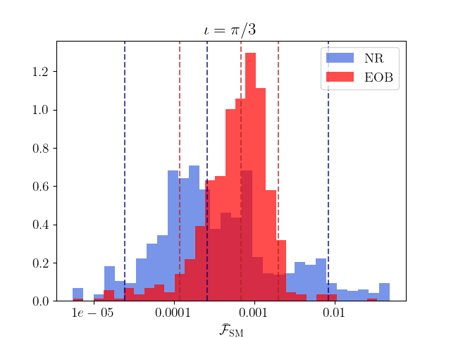
Figure 6: Distribution of $\bar{\mathcal{F}}_{\rm SM}$ between SXS waveforms constructed with all modes up to $\ell=8$ and the same modes except $m=0$ ones (blue) or EOB waveforms constructed with all modes up to $\ell=5$ and the same modes except $m=0$ ones. We consider systems with the same parameters as those examined in Sec. III.2. For a fixed inclination of $\iota=\pi/3$, we find that both sets span the interval $\bar{\mathcal{F}}_{\rm SM}\in[10^{-5},5\times 10^{-2}]$.

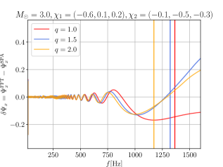
Figure 7: Phase differences between the frequency domain cross polarizations $h_{\times}$ obtained either by twisting SPA-transformed modes or directly via FFT. The three fiducial BNS systems considered have varying mass ratios $q=\{1,1.5,2\}$ and fixed spins, total masses and tidal parameters. Vertical colored lines denote the merger frequency. At merger, the largest phase difference amounts to $\approx-0.2$ radians.

II.5 Higher modes and $m=0$

The higher modes are obtained by twisting the $\ell>2$ spin-aligned modes of TEOBResumS v2. Precessing TEOBResumS computes all modes with $\ell\leq 5$ including the twisted $m=0$ modes. Note that, similarly to most of the currently available approximants, we compute the co-precessing $m<0$ modes by means of symmetry with the $m>0$ modes. This approximation, which is valid in absence of precession of the orbital plane, does not hold when describing precessing systems close to merger Ossokine et al. (2020); Ramos-Buades et al. (2020). Nonetheless, it was found that the effect of employing this approximation is subdominant to other sources of error Ossokine et al. (2020).

The contribution of $m=0$ modes, negligible when dealing with spin-aligned waveforms, can become relevant for precessing binaries.

For example, Fig. 5 shows how the precessing $h^{T}_{\ell,0}$ modes of the $\tt{SXS:BBH:1409}$ NR simulation contribute to the total waveform polarization $h_{+}$ for two binaries with inclinations $\iota=\pi/3$ and $\iota=\pi/2$. While the amplitude of $h^{T}_{\ell,0}$ modes can become as large as that of $h^{T}_{2,2}$ close to merger, the mode sum of $h^{T}_{\ell m}$ with spin-weighted spherical harmonics decreases the overall importance of the $m=0$ modes when computing the polarizations. Nonetheless, the contribution to the amplitude for large-inclination binaries is non-negligible, whereas the phase difference between the $h_{+}$’s obtained with and without the $m=0$ modes oscillates around zero during the inspiral and remains below $\sim 1$ rad at the merger. To systematically quantify the importance of precessing $m=0$ modes, we compute the sky-maximized and SNR-weighted unfaithfulness $\bar{{\cal F}}_{\rm SM}$ between our entire SXS validation set of waveforms (see Sec. III.1 and III.2), constructed by either setting the precessing $m=0$ modes to zero or by considering them in the construction of the polarizations. Fig. 6 shows the distribution of the mismatches computed for binaries with $\iota=\pi/3$. We find that while most of the mismatches obtained are ${\cal O}(10^{-4})$, for some high mass ratio systems $\bar{\mathcal{F}}_{\rm SM}>3\%$. Repeating this analysis with EOB waveforms yields qualitatively similar results, with few mismatches surpassing the $3\%$ threshold. Thus, accurate modelling of the precessing $m=0$ modes is important for very asymmetrical binaries. We note however that current modelling of the twisted $m=0$ modes is not complete as the default TEOBResumS treatment of the spin-aligned $m=0$ modes sets them to zero thus overlooking their contributions in the twist formula (8). We plan to study the effects employing nonzero spin-aligned $m=0$ modes in the future.

II.6 BNS Frequency-domain waveforms

Spin-aligned EOB models can be straightforwardly extended to the frequency domain by applying a stationary phase approximation (SPA) to the multipolar modes $h_{\ell m}(t)$. The frequency domain, spin-aligned modes $\tilde{h}_{\ell m}(f)$ can then be twisted and combined into plus and cross polarization as Pratten et al. (2021):

$$h_{+}= \frac{1}{2}\sum_{\ell\geq 2}\sum_{m^{\prime}>0}e^{im^{\prime}\gamma}\tilde{h}_{\ell m^{\prime}}$$ (22a)

$$\times\sum_{m=-\ell}^{\ell}\Bigl{[}e^{-im\alpha}d^{\ell}_{mm^{\prime}}{}_{-2}Y^{\ell m}+(-1)^{\ell}e^{im\alpha}d^{\ell}_{m-m^{\prime}}{}_{-2}Y^{\ell m\ast}\Bigr{]}\,,$$

$$h_{\times}= \frac{1}{2}\sum_{\ell\geq 2}\sum_{m^{\prime}>0}e^{im^{\prime}\gamma}\tilde{h}_{\ell m^{\prime}}$$ (22b)

$$\times\sum_{m=-\ell}^{\ell}\Bigl{[}e^{-im\alpha}d^{\ell}_{mm^{\prime}}{}_{-2}Y^{\ell m}-(-1)^{\ell}e^{im\alpha}d^{\ell}_{m-m^{\prime}}{}_{-2}Y^{\ell m\ast}\Bigr{]}\,.$$

The sign differences in our expressions with respect to those presented in Ref. Pratten et al. (2021) come from the EOB convention that the phase of the time domain multipoles $h_{\ell m}$ with $m>0$ is positive. Hence, $\tilde{h}_{\ell m}(f)=0$ for $m>0$ and $f<0$. The Euler angles $\alpha,\beta,\gamma$ are all evaluated at the SPA frequencies $2\pi f/m$.

Figure 7 displays the phase difference in the frequency domain of the cross polarization $h_{\times}$ computed between the FFT of precessing TEOBResumS time domain signals and the SPA-based model described above. We consider three nominal BNS systems with fixed spins $\bm{\chi}_{1}=(-0.6,0.1,0.2)$, $\bm{\chi}_{2}=(-0.1,-0.5,-0.3)$ inspiralling from an initial frequency $f_{0}=20$ Hz, tidal polarizability parameters $\Lambda_{1}=\Lambda_{2}=400$, total mass $M=3M_{\odot}$ and mass ratios of 1, 1.5, and 2. For all three cases considered, we find that the phase difference at the merger (represented by the vertical lines) lies below 0.2 rad. The conclusions of Ref. Gamba et al. (2021c) regarding the validity of the SPA up to merger can be applied also to precessing BNS systems. At the same time, the SPA-based model is less computationally expensive than its TD counterpart thanks to the non-uniform time grid which is employed for the inspiral. Moreover, and more importantly, it opens to the possibility of generating waveforms directly over a non-uniform frequency grid, optimized for PE, allowing the application of techniques such as relative binning Zackay et al. (2018) or multibanding Vinciguerra et al. (2017).

III Validation

In this section we compare our EOB model to (i) the set of $99$ precessing ${\tt SXS}$ simulations also employed in Ref. Pratten et al. (2020), supplemented with the longer precessing simulations ${\tt SXS:BBH:1389}$ to ${\tt SXS:BBH:1409}$, and (ii) 5000 ${\tt NRSur7dq4}$ (henceforth NRsur) waveforms, spanning $q\in[1,4]$ and $|\chi_{i}|\in[0.1,0.8]$ yielding a range of $-0.8\leq\chi_{\text{eff}}\leq 0.8$ and $0.0\leq\chi_{p}\leq 0.8$. We compute the sky-averaged faithfulness (see Sec. IV of Ref. Harry et al. (2016)) for all considered templates. Then, for a selected number of systems, we align the time-domain polarizations and compute the cumulative phase difference of the waveform $h=h_{+}-ih_{\times}$. Overall, we find that the maximum mismatch between TEOBResumS and ${\tt SXS}$ is obtained for very asymmetric, highly spinning binaries. The same statement holds for ${\tt NRsur}-\texttt{TEOBResumS}{}$ mismatches.

III.1 Faithfulness

The Wiener product between two time domain waveform templates $a(t),b(t)$ is defined as

$$(a,b)=4\text{Re}\int\frac{\tilde{a}^{*}(f)\tilde{b}(f)}{S_{n}(f)}\,\mathrm{d}f,$$

where $S_{n}(f)$ is the power spectral density (PSD) of the detector and $\tilde{a},\tilde{b}$ denote the Fourier transform of the waveforms. The agreement between a target model $s$ and a generic template $h$ is usually quantified through the faithfulness (or match) $\mathcal{F}$, defined as the normalized inner product between $s$ and $h$, maximized over the reference time and phase $t_{0},\varphi_{0}$:

$$\mathcal{F}=\max_{t_{0},\varphi_{0}}\frac{(s,h)}{\sqrt{(s,s)(h,h)}}.$$ (23)

However, when the template waveform incorporates higher modes or if the system is precessing, this definition is not completely independent of the extrinsic parameters of the binary. In general, the target and template waveforms are obtained from the plus and cross polarizations as:

$$\begin{split}k_{i}&=F_{+}(\theta^{i},\phi^{i},\psi^{i})\;k_{+}(\iota^{i},\varphi_{0}^{i},t_{0}^{i},\Theta^{i})\\ &+F_{\times}(\theta^{i},\phi^{i},\psi^{i})\;k_{\times}(\iota^{i},\varphi_{0}^{i},t_{0}^{i},\Theta^{i}),\end{split}$$ (24)

where $i=s,h$ and $\theta,\phi,\psi,\iota,\Theta$ are, respectively, the right ascension, declination, polarization, inclination, and intrinsic parameters (masses, spins, tidal parameters etc.) of the binary system. Equation (24) can be rearranged into

$$\begin{split}k_{i}=\mathcal{A}(\theta^{i},\phi^{i})[&\cos\kappa(\theta^{i},\phi^{i},\psi^{i})k_{+}(\iota^{i},\varphi_{0}^{i},t_{0}^{i},\Theta^{i})\\ &+\sin\kappa(\theta^{i},\phi^{i},\psi^{i})k_{\times}^{i}(\iota^{i},\varphi_{0}^{i},t_{0}^{i},\Theta^{i})]\,,\end{split}$$ (25)

where $\kappa$ denotes the effective polarizability and

$$e^{i\kappa(\theta,\phi,\psi)} =\left[F_{+}(\theta,\phi,\psi)+iF_{\times}(\theta,\phi,\psi)\right]/\mathcal{A}(\theta,\phi)\,,$$ (26)

$$\mathcal{A}(\theta,\phi) =\sqrt{F^{2}_{+}(\theta,\phi,\psi)+F^{2}_{\times}(\theta,\phi,\psi)}\,.$$ (27)

When only $(2,\pm 2)$ modes are considered, it can be shown that Eq. (23) depends on extrinsic parameters only through overall amplitude and phase factors. On the other hand, when higher modes are considered, the dependence on the extrinsic quantities is nontrivial.

We define the (template) sky-maximized (SM) faithfulness between the target strain and the waveform template as

$$\mathcal{F}_{\text{SM}}=\max_{t_{0}^{h},\varphi_{0}^{h},\kappa^{h}}\frac{(s,h)}{\sqrt{(s,s)(h,h)}},$$ (28)

where we dropped the explicit depencence on intrinsic and extrinsic parameters in the right hand side. Accordingly, the unfaithfulness is given by $\bar{\mathcal{F}}_{SM}=1-{\mathcal{F}}_{SM}$. We follow the procedure outlined in Sec. IV of Ref. Harry et al. (2016). The maximization over $\kappa$ is performed analytically, while $t_{0}$ is maximized via the inverse FFT. The maximization over the reference phase $\varphi_{0}$ is performed numerically through a dual annealing algorithm, similar to what is done in Ref. Pratten et al. (2021). Finally, we mention that for precessing systems one additional degree of freedom remains: the freedom to perform a rigid rotation of the in-plane spin components about the initial $\hat{z}$ axis, which is equivalent to choosing different initial conditions for the $\alpha$ (and $\gamma$) Euler angles. We further maximise $\mathcal{F}_{\text{SM}}$ over such a rotation by once more relying on a dual annealing algorithm. We note that this procedure differs from the one employed in Ref. Ossokine et al. (2020), where instead the initial (reference) frequency is varied, and the initial in-plane spin components are kept fixed to their nominal target value.

Once $\mathcal{F}_{\text{SM}}$ (or, equivalently, $\bar{\mathcal{F}}_{\text{SM}}$) is computed as described, we normalize it over the SNR of the signal and further average over the sky angles of the target waveform, in order to completely marginalize over any dependence of the mismatch on the sky position and obtain values which depend exclusively on the intrinsic parameters of the source. We consider $N_{\varphi}$ values of $\varphi_{0}^{s}\in[0,2\pi)$ and $N_{\kappa}$ values of $\kappa^{s}\in[0,2\pi)$, and present the average value over $N_{\varphi}\times N_{\kappa}$ values.

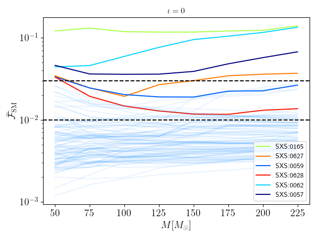
Figure 8: NR/EOB mismatch, $\bar{\mathcal{F}}_{\rm SM}$, for the 99 SXS short precessing simulations computed with strain mode content $\ell\leq 4+(5,\pm 5)$, plotted as a function of the total mass of the system and computed with a fixed inclination of the binary of $\iota=\{0,\pi/3,\pi/2\}$ (top, middle and bottom panels, respectively). A total of ten configurations have $\bar{\mathcal{F}}_{\rm SM}$ which reaches up to $3\%$. The dashed horizontal lines in each panel mark the $3\%$ and $1\%$ thresholds.

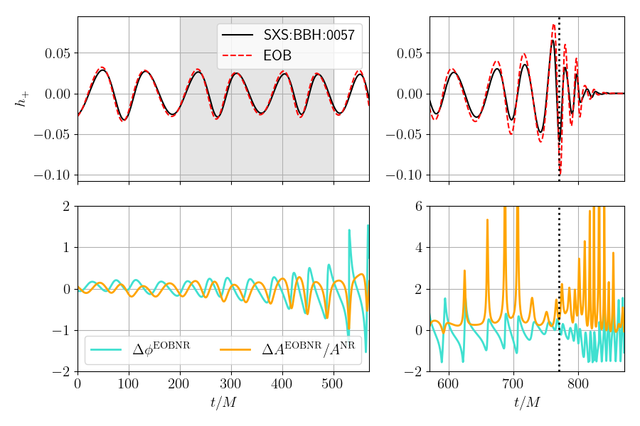
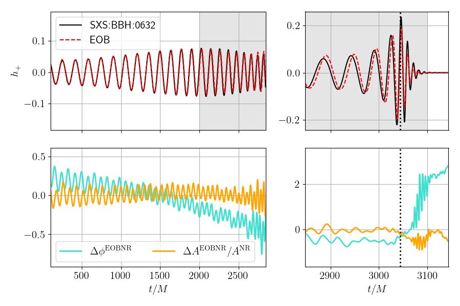
Figure 9: Visual comparison between the $h_{+}$ NR waveforms (black, solid curves) computed from SXS:BBH:0057 (left panel) and SXS:BBH:0632 (right panel) and the TEOBResumS waveforms obtained with the same intrinsic parameters (red, dashed), inclination $\iota=\pi/3$ and all modes with $\ell\leq 4$. The phase difference $\Delta\phi^{\rm EOBNR}=\phi_{\rm NR}-\phi_{\rm EOB}$ is shown in cyan, and the relative amplitude error $\Delta A^{\rm EOBNR}/A^{\rm NR}$ in orange. Merger is indicated by a black dotted line. The waveforms are aligned by minimizing the phase difference in the time window highlighted in gray, see Eq. (30) of Ref. Dietrich et al. (2019). Both systems are characterized by very large in-plane spins at their initial reference frequency, with $\tt SXS:BBH:0057$ also having $q>5$. While the phase difference oscillates during the inspiral and generally remains below  1 rad, the dephasing and the amplitude relative differences increase at merger, indicating that an improved description of the final moments of the coalescence will be required.

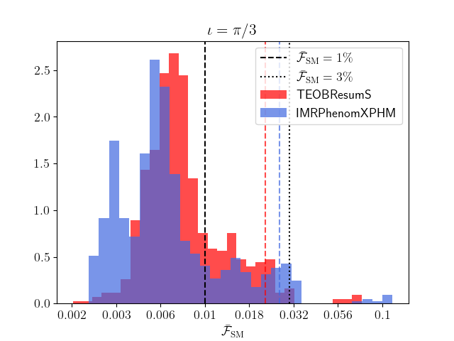
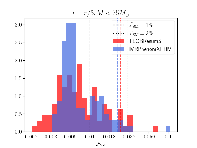
Figure 10: Left panel: the distribution of NR/TEOBResumS and NR/IMRPhenomXPHM mismatches for the 99 SXS short precessing simulations of Fig. 8, at a fixed binary inclination of $\iota=\pi/3$. The black dashed and the dotted black vertical lines mark the $1\%$ and $3\%$ thresholds, and dashed colored lines the $95^{\rm th}$ percentiles. We find that the performance of $\tt IMRPhenomXPHM$ is comparable to that of our EOB approximant, with $\bar{\mathcal{F}}_{\text{SM}}^{\rm EOB}$ falling in the range $0.002-0.06$ with median at $0.007$, and $\bar{\mathcal{F}}_{SM}^{\rm XPHM}$ falling within the interval $0.002-0.1$ and having a median of $0.005$. Right panel: the same plot as above, with total masses restricted to below $75M_{\odot}$. Overall, TEOBResumS performs slightly better than $\tt IMRPhenomXPHM$ for lower masses, and slightly worse for higher ones.

III.2 BBH IMR EOB/NR comparison

To validate the performance of our model, we compare our waveforms with a set of selected SXS NR simulations. In particular, we focus on two different sets: 99 “short” waveforms, with $\chi_{p}\lesssim 0.84$, $\chi_{\rm eff}\in[-0.45,0.65]$ and $q\lesssim 6$, and 21 “long” simulations with $\chi_{p}\lesssim 0.49$, $\chi_{\rm eff}\in[-0.2,0.3]$ and $q\lesssim 4$, spanning from $\sim 60$ to $\sim 146$ orbits. To translate the NR data from the NR frame into the source frame described in Sec. I, we make use of the public catalog tools available at sxs and described in, e.g., Ref. Schmidt et al. (2017). For all unfaithfulness computations, we consider total detector-frame masses $M\in[50,225]M_{\odot}$, employ the zero-detuned high-power PSD of Ref. aLI and average $\bar{\mathcal{F}}_{\rm SM}$ over a grid $\kappa^{\rm NR}=\{0,\pi/2,\pi,3/2\pi\}$ and $\varphi_{0}^{\rm NR}=\{0,2\pi/5,4\pi/5,6\pi/5,8\pi/5\}$. We perform our computations over the frequency range $[f_{\rm min},2048]$ Hz, where $f_{\rm min}$ is the initial GW frequency of the NR waveform, expressed in physical units.

III.2.1 “Short” SXS simulations

Figure 8 shows the sky-averaged $\bar{\mathcal{F}}_{\rm SM}$ as a function of the total binary mass for three different choices of the binary inclination, $\iota=\{0,\pi/3,\pi/2\}$. We find that when $\iota=0$ ($\pi/3,\pi/2$), all but six (four) notable simulations the EOB/NR unfaithfulness lies below the $3\%$ threshold for all values of masses considered, and that $80\%$ ($76\%,68\%$) of the averaged $\bar{\mathcal{F}}_{\rm SM}$ computed are smaller than $1\%$. The configurations for which the EOB/NR faithfulness lies above the $3\%$ threshold are highly asymetrical $(q>5)$ or strongly precessing $(\chi_{\rm p}>0.7)$ systems, with ${\tt SXS:BBH:0165}$ being the most challenging one, as it is a $(q,\chi_{\rm eff},\chi_{\rm p})=(6,-0.45,0.77)$ coalescence. In Fig. 9 we consider two more of these systems ($\tt SXS:BBH:0057$ and $\tt SXS:BBH:0632$), and align the time-domain NR and EOB waveforms by minimizing their phase difference $\Delta\phi^{\rm EOBNR}=\phi^{\rm NR}-\phi^{\rm EOB}$ over a chosen time-window (see e.g. Dietrich et al. (2019)). We find that the EOB waveform correctly captures the behavior of the NR waveform up to few orbits before merger, where differences in phase and amplitude start to grow.

For comparison, we also compute $\bar{\mathcal{F}}_{\rm SM}$ between the set of NR simulations here considered and the waveform approximant $\tt IMRPhenomXPHM$ Pratten et al. (2021), with fixed inclination $\iota=\pi/3$. Figure 10 shows the results of this calculation. We find that $\bar{\mathcal{F}}_{SM}^{\rm EOB}$ varies between $\sim 0.002$ and $0.06$, with the distribution median peaking at $0.007$; while $\bar{\mathcal{F}}_{SM}^{\rm XPHM}$ spans the interval $\sim 0.002$ to $0.1$, with a median of $0.005$.

Overall, the two approximants give consistent results, with TEOBResumS generally performing marginally worse at high masses, and marginally better for $M<75M_{\odot}$.

III.2.2 “Long” SXS simulations

Figure 11 once more shows the sky-averaged $\bar{\mathcal{F}}_{\rm SM}$ as a function of the total binary mass for two different choices of the binary inclination, $\iota=0,\pi/3,\pi/2$. The mismatches behave similarly to what we described above in the sense that they generally degrade for increasing magnitude of in-plane spins and growing inclinations. This well-known fact can be appreciated also from Fig. 12, where we align the NR waveform ${\tt SXS:BBH:1397}$ and the corresponding EOB waveform. We compute the phase difference $\Delta\phi^{\rm EOBNR}$ between the two, and find that for $\iota=0$ it is constantly smaller than $0.1$ rad during the inspiral, growing to $\sim 0.6$ rad after merger. For $\iota=\pi/3$ the phase difference displays larger oscillations, which are however always smaller than $0.5$ rad. The relative difference in the amplitude $\Delta A^{\rm EOBNR}/A^{\rm NR}=(A^{\rm NR}-A^{\rm EOB})/A^{NR}$, instead, degrades after merger for the $\iota=\pi/3$ case. Nonetheless, for the case considered the behavior of both the EOB phase and amplitude remain correct during the merger.

Overall we find that all the mismatches computed lie below $3\%$ for the inclinations considered, and $93\%$ ($98\%$, $87\%$) below $1\%$ for $\iota=0$ ($\iota=\pi/3,\pi/2$).

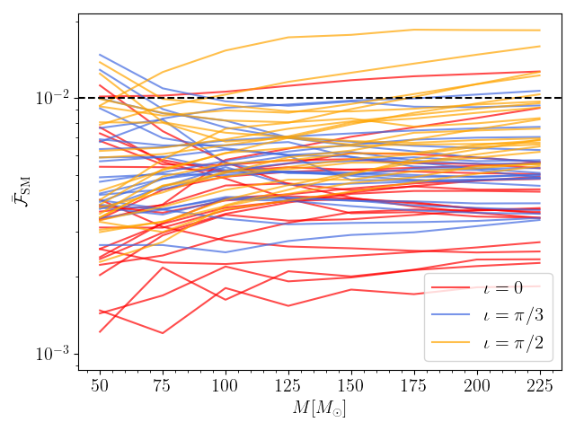
Figure 11: NR/EOB mismatch for the SXS long precessing simulations 1389 to 1409, plotted as a function of the total mass of the system and computed with a fixed inclination of the binary of $\iota=0,\pi/3,\pi/2$ (red, blue and orange lines, respectively). The dashed black horizontal line marks the $1\%$ threshold. No simulations have $\bar{\mathcal{F}}_{\rm SM}>3\%$ for any of the considered inclinations.

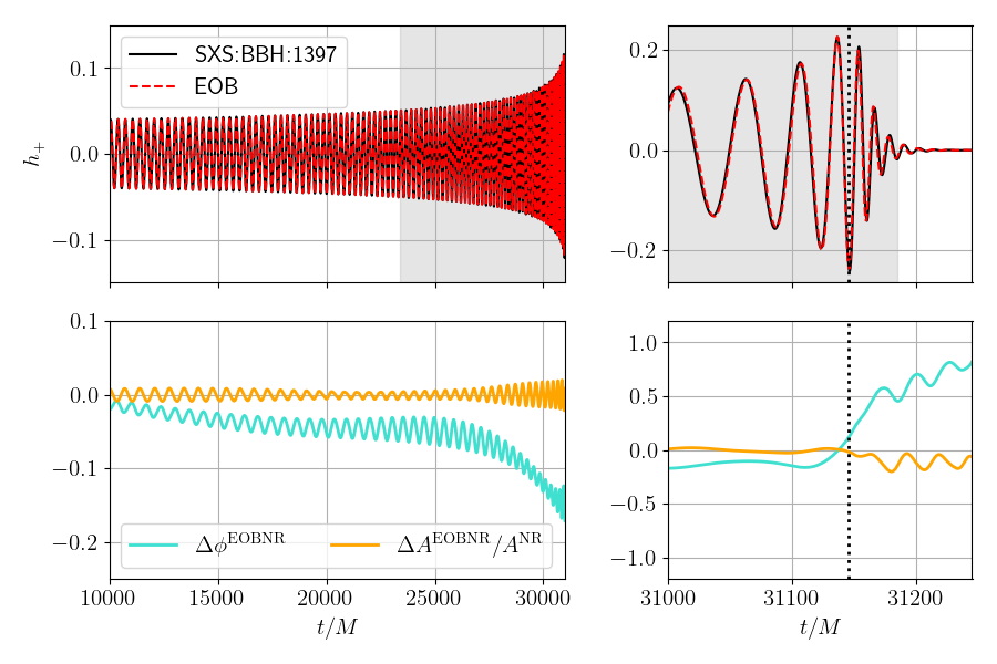
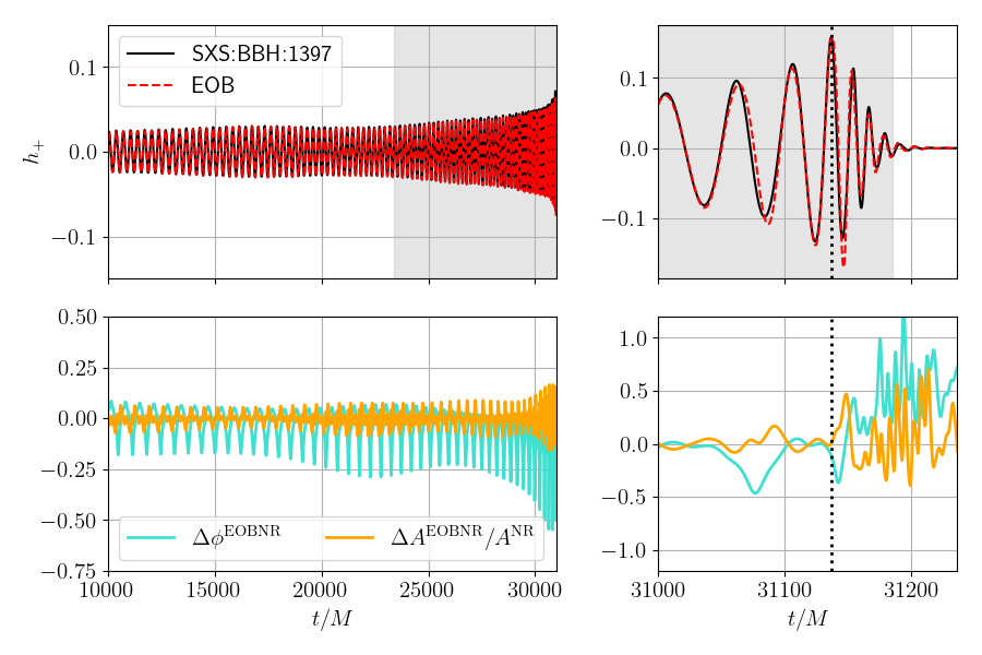
Figure 12: Visual comparison between the $h_{+}$ waveform computed from SXS:BBH:1397 (black, solid curves) with $\ell\leq 4$ and the TEOBResumS waveform obtained with the same intrinsic parameters (red, dashed) for two different inclinations, $\iota=0$ (left panel) and $\iota=\pi/3$ (right panel). The phase difference $\Delta\phi^{\rm EOBNR}=\phi_{\rm NR}-\phi_{\rm EOB}$ is shown in cyan, and the relative amplitude error $\Delta A^{\rm EOBNR}/A^{\rm NR}$ in orange. Merger is indicated by a black dotted line. The waveforms are aligned by minimizing the phase difference in the time window highlighted in gray. As the inclination increases, so do the importance of higher modes and the amplitude modulations due to precession.

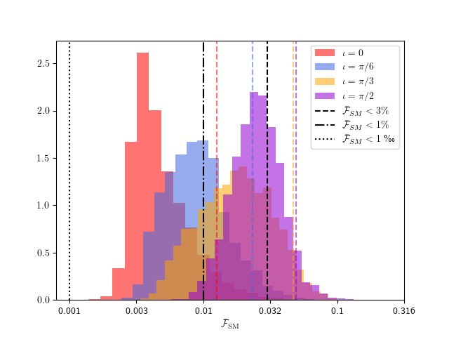
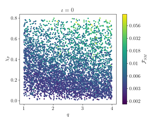
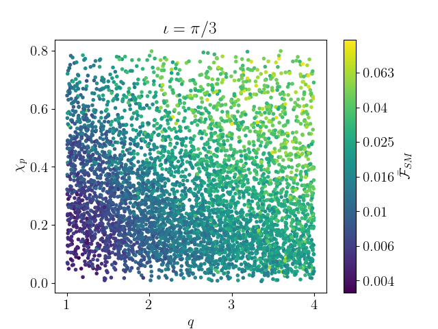
Figure 13:  Top panel: NRSur7dq4/TEOBResumS sky maximized $\ell\leq 4$ mismatch for 5000 systems with $q\in[1,4]$, spin magnitudes $\chi_{i}\in[0.1,0.8]$ and random spin directions, computed from an initial frequency range of 20 to 37.5 Hz with the aLIGO design PSD noise curve up to $1024$ Hz. The dotted, dot-dashed, and dashed vertical black lines mark unfaithfulness of $1$‰, $1\%$, and $3\%$, respectively. The colored, dashed vertical lines mark the 95th percentiles for the four distributions. Middle and bottom panels: the behavior of the mismatch over the $\{q,\chi_{p}\}$ parameter space for inclinations of 0 and $\pi/3$. The higher unfaithfulness values are obtained for highly asymmetrical systems, with large in-plane spins (high $\chi_{p}$) and mass ratios of $q>2$.

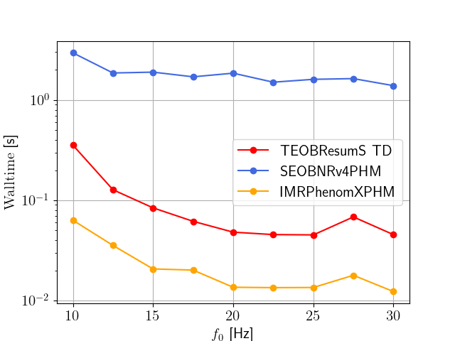
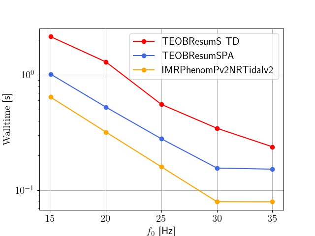
Figure 14: Left panel: BBH evaluation time for a $q=1,M=60M_{\odot}$ precessing system containing the $(\ell,m)=(2,1),(2,2),(3,2),(3,3),(4,4)$ modes. Three different state of the art approximants are considered: TEOBResumS, ${\tt IMRPhenomXPHM}$ and ${\tt SEOBNRv4PHM}$. TEOBResumS  is approximately three times slower than ${\tt IMRPhenomXPHM}$, and up to an order of magnitude faster than ${\tt SEOBNRv4PHM}$. Right panel: BNS evaluation time for a $q=1,M=3.5M_{\odot}$ precessing system, whose waveform is constructed with the $(2,2)$ mode. TD denotes the standard time domain TEOBResumS model with SPA denoting the frequency domain version of Sec. II.6

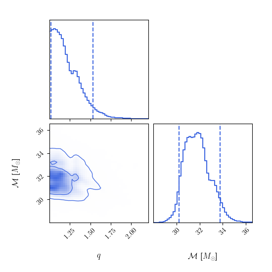
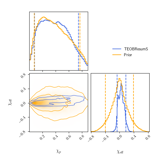
Figure 15: Posteriors for chirp mass, mass ratio and spins obtained by analyzing the GW150914 data with TEOBResumS, as discussed in Sec. IV.1. For comparison, we also plot the prior distributions for $\chi_{\rm eff}$ and $\chi_{p}$. As expected, the posterior distribution of $\chi_{p}$ is consistent with its prior. The masses obtained in our analysis are consistent with the ones previously reported in Ref. Breschi et al. (2021), but the uncertainties on $q$ and $\mathcal{M}$ are larger. This is due to the addition of four degrees of freedom, namely the in-plane spin components.

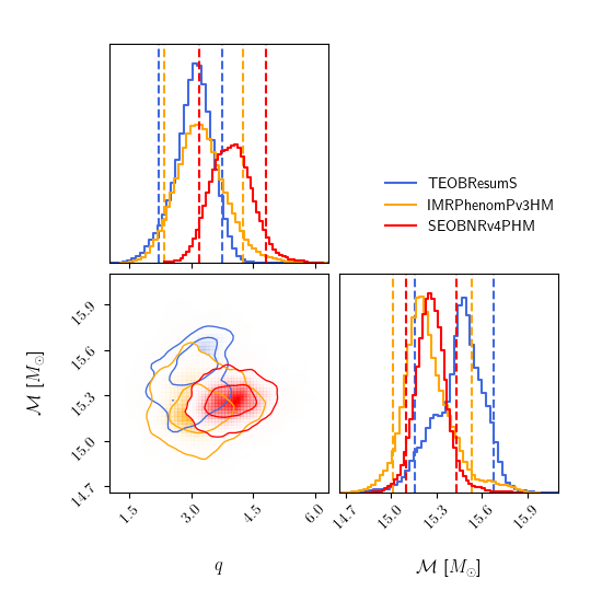
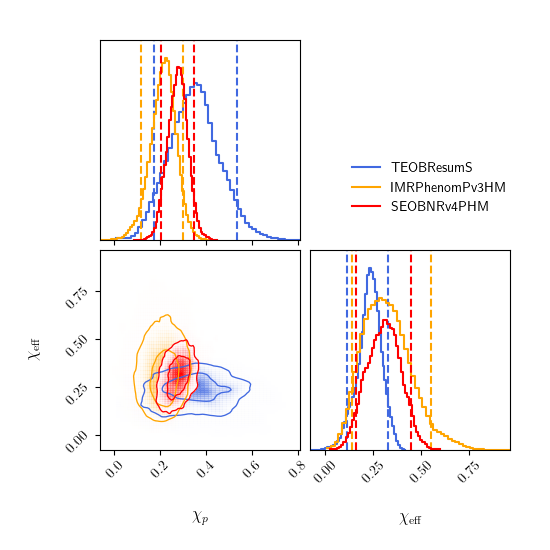
Figure 16: Posteriors for chirp mass, mass ratio and spins obtained by analyzing the GW190412 data with TEOBResumS, as discussed in Sec. IV.2. We compare our results to the public LVC posteriors obtained with the precessing models SEOBNRv4PHM and IMRPhenomPv3HM. The results of our analysis are broadly consistent with the ones obtained by LVC, although some model systematics are clearly present between the three approximants.

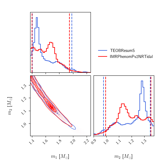
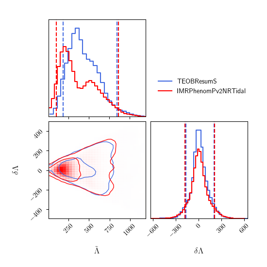
Figure 17: Marginalized, two dimensional posteriors for detector frame masses (left) and tidal parameters (right) for GW170817, obtained with the precessing TEOBResumS model or the phenomenological ${\tt IMRPhenomPv2NRTidal}$ model, from the analysis of Ref. Abbott et al. (2019b). The $90\%$ intervals are compatible between the two models. We not that the ${\tt IMRPhenomPv2NRTidal}$ posteriors for $\tilde{\Lambda}$ display some bimodalities, which are due to the higher frequency cutoff employed for the analysis.

III.3 Comparison with NRSur7dq4

To extend the comparison to a larger number of binaries, we additionally computed $\bar{\mathcal{F}}_{\rm SM}$ between our model and the NR surrogate model $\tt{NRSur7dq4}$ using all modes with $\ell\leq 4$. We considered $5000$ systems with $q\in[1,4]$, which is the calibration region of the surrogate, and spin magnitudes $\chi_{1,2}\in[0.1,0.8]$ with uniformly distributed spin vector polar angles $\theta_{1,2}\in[0,\pi)$ and azimuthal angles $\phi_{1,2}\in[0,2\pi)$. We set the initial GW frequency to 20 Hz for $M\geq 100M_{\odot}$ and to a linearly decreasing function of $M$ from 37.5 to 20 Hz as $M$ increases from 40 to $100\,M_{\odot}$. We do this because the surrogate can at most yield waveforms of length $4300M$ Varma et al. (2019b) so the lighter-mass inspirals need to start from higher frequencies. Figure 13 shows the distributions of the unfaithfulness obtained for inclinations of $\iota=0,\pi/6$,$\pi/3$ and $\pi/2$. We find that, for $\iota=0$, $98.8\%$ of the systems considered have unfaithfulness below $3\%$ and $87.8\%$ below $1\%$, with a global distribution spanning the range $\bar{\mathcal{F}}_{\rm SM}\in[0.0027,0.04]$ with median $0.0046$.

As previously observed, the situation worsens as the inclination increases, with $\bar{\mathcal{F}}_{\rm SM}\in[0.003,0.05]$ for $\iota=\pi/6$, $\bar{\mathcal{F}}_{\rm SM}\in[0.003,0.1]$ for $\iota=\pi/3$ and $\bar{\mathcal{F}}_{\rm SM}\in[0.006,0.14]$ for $\iota=\pi/2$.

For $\iota=\pi/3$, only $80\%$ ($21\%$) of the total mismatches are below the $3\%$ ($1\%$) threshold. The degradation of the unfaithfulness is observed especially for asymmetric binaries with large $\chi_{p}$ as can be discerned by comparing the middle and bottom panels of Fig. 13.

III.4 Waveform evaluation timing

We now test the computational efficiency of our EOB model, and compare it to other state of the art precessing approximants for BBH and BNS coalescences, ${\tt SEOBNRv4PHM}$, ${\tt IMRPhenomXPHM}$ and ${\tt IMRPhenomPv2NRTidalv2}$. We choose one reference equal mass BBH binary, with $M=60M_{\odot}$ and $\bm{\chi}_{1}=(-0.6,0.1,0.2)$, $\bm{\chi}_{2}=(0.1,-0.5,-0.3)$, and a list of initial frequencies $f_{0}=\{10,12.5,15,17.5,20.,22.5,25,27.5,30\}$ Hz. For each initial frequency $f_{0}^{i}$ we calculate the average time (over 20 repetitions) needed to evolve the binary and produce the $h_{+}$ and $h_{\times}$ polarization. This process is then repeated for a BNS configuration with $q=1,M=2.8M_{\odot}$ and same spins as the previous BBH system, and a choice of initial frequencies $f_{0}=\{15,20,25,30,35\}$ Hz. We performed this test on a Huawei MateBook 14 with AMD Ryzen 5 2500U processors and 8 Gb RAM.

The results are displayed in Fig. 14. We find that, for BBH systems, TEOBResumS is approximately three to four times slower than ${\tt IMRPhenomXPHM}$ and about one order of magnitude faster than ${\tt SEOBNRv4PHM}$. For BNS systems, instead, the FD model is about two times faster than its TD counterpart, and two times slower than the phenomenological $\tt IMRPhenomPv2NRTidalv2$. We highlight that the main evaluation cost for both the TD and FD TEOBResumS models comes from the twisting procedure itself, rather than from the solution of the two (PN and EOB) dynamics ODE systems.

IV Parameter estimation

We demonstrate possible applications of our model by performing PE on real GW data. We re-analyze the data of GW150914 and GW190412, and show that the posteriors obtained are consistent with those presented in, e.g., Refs. Abbott et al. (2019b, 2021b). Then, we analyze GW170817  Abbott et al. (2017d, 2019a, 2018) and compute the radius of a NS of mass $M\in[1.4,2.1]M_{\odot}$ using the fits of Ref. Godzieba and Radice (2021). All of our PE studies are performed with the bajes pipeline Breschi et al. (2021) and the ${\tt dynesty}$ Speagle (2020) sampler.

IV.1 GW150914

GW150914 Abbott et al. (2016a, 2019b) was the first BBH event observed by the LIGO collaboration. For our study, we consider 8 seconds of data centered around the GPS time of the event. We employ 4096 livepoints, and analyze the frequencies between $20$ and $1024$ Hz. We fix the sampling rate to 4096 Hz, and sample the component masses enforcing that the chirp mass lies in $\mathcal{M}\in[12.3,45]M_{\odot}$, the mass ratio $q\in[1,8]$, and the spin magnitudes $|\chi_{i}|\in[0,0.89]$ with $i=1,2$ with an isotropic prior for the tilt angles. We consider all modes up to $\ell=4$, and marginalize over the timeshift. Finally, we employ 10 calibration nodes, and the PSD given in Ref. Abbott et al. (2019b). Fig. 15 displays the posteriors we recovered from our analysis. We find that $\mathcal{M}=31.7^{+2.0}_{-1.5}M_{\odot}$, $q=1.17^{+0.36}_{-0.16}$, $\chi_{\rm eff}=0.04^{+0.09}_{-0.08}$ and $\chi_{\rm p}=0.38^{+0.37}_{-0.29}$. Our results are consistent with the analyses presented in Refs. Abbott et al. (2016a, c, 2019b), performed with other approximants, and with the PE conducted in Ref. Breschi et al. (2021), which employed the non-precessing version of TEOBResumS. The posteriors of $\chi_{\rm p}$ are consistent with the prior as GW150914 displays no evidence of precession. Notably, the introduction of additional spin components widens the credible intervals on the component masses with respect to the analysis of Ref. Breschi et al. (2021), obtained with the same approximant and similar settings.

IV.2 GW190412

GW190412 was the first highly asymmetrical BBH event ($q\approx 3-4$), which was also one of the “louder” events of O3a with an SNR of $~{}19$ Abbott et al. (2021b, 2020b). The original LVC data analysis has yielded well constrained imprints of spin precession with $0.15\lesssim\chi_{\text{p}}\lesssim 0.5$ and $\theta_{1}=0.80^{+0.52}_{-0.36}$ Abbott et al. (2021b), support for $\chi_{\text{eff}}>0$ with 95% credibility Abbott et al. (2021b), and clear evidence of the subdominant modes carrying a significant portion of the signal SNR. A number of following studies have further improved on the original analysis by investigating in more detail the effects of the higher modes Islam et al. (2021) and of the chosen priors Colleoni et al. (2021) on the PE. The same works also carried out studies to understand the differences observed when different waveform models are employed to analyze the signal. Although such detailed investigations lie beyond the scope of this paper, it is clear that the exceptional nature of GW190412 makes it very desirable to analyze with TEOBResumS.

We employ 4096 livepoints and analyze the frequencies between $20$ and $1024$ Hz with a fixed sampling rate of $4096$ Hz. We sample in the component masses, requiring that the chirp mass falls in $\mathcal{M}\in[8,20]M_{\odot}$ and the mass ratio $q\in[1,10]$. We sample in spin magnitudes $|\chi_{i}|\in[0,0.89]$ with $i=1,2$, enforcing an isotropic prior for the tilt angles. Once again, we consider all modes up to $\ell=4$, and marginalize over the timeshift.

Posteriors for the masses and spins are plotted in Fig. 16. We compare the results obtained in our PE with the publicly available LVC posterior samples, obtained with the two independent models ${\tt SEOBNRv4PHM}$ Ossokine et al. (2020) and ${\tt IMRPhenomPv3HM}$ Khan et al. (2019a). We find that TEOBResumS gives estimates of GW190412 parameters that are overall consistent with those computed from the other two approximants. We obtain a slightly larger chirp mass, and overall wider $\chi_{p}$ and tighter $\chi_{\rm eff}$ posteriors.

IV.3 GW170817

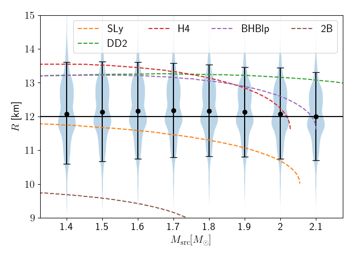
Figure 18: Marginalized posterior distributions of $R(M)$ computed via the tidal parameters and source masses obtained from our GW170817 analysis and the fits of Ref. Godzieba and Radice (2021). Overlayed, we also display the $R(M)$ relations for a handful of well-known equations of state.

GW170817 was the first BNS inspiral/merger event. To date, it is still the loudest detected GW event with an SNR of 32 Abbott et al. (2017d). Though observations from millisecond pulsars yield at most dimensionless spins of $\chi\approx 0.5$ Hessels et al. (2006) and the fastest observed neutron star spin in electromagnetically observed binary pulsars is $\chi\lesssim 0.05$ Kramer and Wex (2009); Stovall et al. (2018), the spins of the components of GW170817 are not well constrained Abbott et al. (2017d, 2019b). For our re-analysis we employ 6000 livepoints and consider 128 seconds around the GPS time of the event, analyzing the frequencies between $20$ and $1024$ Hz to minimize waveform systematics Gamba et al. (2021c). We sample the component masses imposing that $\mathcal{M}\in[1.1,1.3]M_{\odot}$ and $q\in[1,3]$. The dimensionless spin magnitudes are sampled in the interval $[0,0.89]$, with an isotropic prior for the tilt angles. We sample the dimensionless tidal deformabilities $\Lambda_{1}$, $\Lambda_{2}$ over a uniform prior $[5,5000]$. Figure  17 displays the marginalized, two-dimensional posteriors for the detector masses $m_{1}$, $m_{2}$ of the neutron stars and the tidal parameters $\tilde{\Lambda}$ and $\delta\Lambda$, which parameterize the LO and NLO tidal corrections to the PN GW phase Wade et al. (2014). The masses are slightly bimodal. This effect is not unexpected, and has already been previously observed Abbott et al. (2019a, b). Evidently, it is related to the modelling of spin precession: on the one hand, allowing spin magnitudes to vary in the large interval $[0,0.89]$ increases the correlations between spins and mass ratio; on the other hand, precession effects can more easily fit features of the data which might be due to the noise. This event too, much like GW150914, does not display evidence for precession or spinning components. Indeed, we find that $\chi_{p}$ is consistent with its prior, and $\chi_{\rm eff}=0.01^{+0.04}_{-0.02}$. Finally, we measure $\tilde{\Lambda}=406^{+238}_{-150}$. This value is marginally larger than the one obtained with the IMRPhenomPv2NRTidal model, consistently with Ref. Gamba et al. (2021b), but slightly smaller than the one obtained with the aligned spin model. By employing the fits of Ref. Godzieba and Radice (2021), we map the source frame masses and the $\tilde{\Lambda}$ into posteriors for the radius $R$ of a NS with mass in $[1.4,2.1]M_{\odot}$ (See Fig.  18). Over this mass interval we find that the fits give values of $R$ which are weakly dependent on the mass of the neutron star, and $R\sim 12.0^{+1.5}_{-1.2}$ km.

V Conclusions

In this work we have presented a new efficient multipolar EOB model for generic-spin binaries

The model presented builds on the previous work of Ref. Akcay et al. (2021) and improves it by including a description for merger and ringdown, higher modes and time-evolving projected spin components. We also constructed an inspiral-merger frequency domain model for precessing BNS systems, which can incorporate all the advancements added to the time domain approximant, and is – to our knowledge – the first multipolar, tidal and precessing frequency domain approximant for these systems.

We have investigated different realizations of radiation reaction included in the spin dynamics via the $\dot{\omega}(\omega)$ relation. By comparing hybrid EOB-PN expressions with a pure PN expression and the “aligned” EOB relation, we observed that the PN expression for $\dot{\omega}(\omega)$ employed in the previous work provides a satisfactory description of the EOB radiation reaction. We also presented a preliminary investigation of the importance of $m=0$ modes in asymmetrical binaries, showing that the contribution of the $h^{T}_{\ell,0}$ modes to the total waveform polarizations is non-negligible close to merger.

We then validated TEOBResumS IMR BBH model using a total of $120$ SXS simulations, spanning a large portion of the precessing BBHs parameter space. We found that $96\%$ ($99\%$, $98\%$) of the total mismatches lie below the $3\%$ unfaithfulness threshold for $\iota=0$ ($\iota=\pi/3,\pi/2$). We also computed the mismatch between a subset of the same SXS simulations and the state-of-the-art phenomenological waveform approximant $\tt IMRPhenomXPHM$. We found good consistency between the mismatches obtained with the two waveform models. A similar comparison was performed against the NR surrogate ${\tt NRSur7dq4}$: when considering a large number of systems, which cover the surrogate’s parameter space, we found that $98.8\%$ ($80\%$, $67\%$) of the systems considered have unfaithfulness below $3\%$ and $87.8\%$ ($21\%$, $2\%$) below $1\%$ for $\iota=0$ ($\iota=\pi/3,\pi/2$). The worsening of the unfaithfulness for increasing inclination is expected, as for more edge-on binaries geometrical effects enhance the importance of higher modes and precession, which in turn deteriorate the EOB-NR agreement during the merger and ringdown phases of the coalescence.

Finally, we applied the model to the PE of three real LVC signals, namely GW150914, GW190412 and GW170817, and obtained results consistent with currently published analyses by relying on the $\tt bajes$ PE infrastructure and the ${\tt dynesty}$ sampler. GW150914 and GW170817 display no evidence for precession, with $\chi_{p}$ closely following its prior distribution. Conversely, GW190412 is clearly found to be an asymmetrical, mildly precessing system with mass ratio $q\sim 3$ and $\chi_{\rm p}\sim 0.35$, $\chi_{\rm eff}\sim 0.25$. Such values are compatible with the ones recovered by the LVK collaboration employing the precessing waveform approximants $\tt SEOBNRv4PHM$ and $\tt IMRPhenomPv3HM$. Marginal differences due to waveform systematics are nonetheless found in $\chi_{p}$ and $\chi_{\rm eff}$: we recover a tighter posterior distribution of the latter and a wider distribution of the former, as well as a slighty larger chirp mass. Critically, these studies demonstrate that $\tt TEOBResumS$ can be directly applied to PE, even of computationally challenging BNS systems, without the need for additional surrogates or reduced order models.

In spite of the satisfactory performance of the model for current detectors, some work remains to be done in view of the continuously-increasing sensitivity of the instruments. In particular, the degradation of the performance of the model at high masses seen in Fig. 8 indicates the need for an improved merger-ringdown description of the precessing waveform. This could come from a combination of three different yet complementary avenues: (i) an improved description of the ringdown of spin-aligned $(\ell,m)\neq(2,2)$ modes; (ii) a more accurate model for the evolution of the Euler angles $\alpha$, $\beta$ beyond the merger; (iii) an improved (analytical) fit for the remnant spin $\chi_{f}$ (see Fig. 4).

Regarding the first point, in particular, we mention that the Achille’s heel of the aligned-spin TEOBResumS is the modeling of the $(\ell,m)=(2,1)$ mode, which is known to become inaccurate close to merger for large spins anti-aligned with the orbital angular momentum ($\chi^{z}_{i}<-0.8$) Nagar et al. (2020). This known issue is potentially even more important for precessing systems. That is because, clearly, the twisted modes are obtained as a superposition of spin-aligned multipoles. Hence, the $(2,1)$ mode directly affects also the $(2,2)$ and $(2,0)$ multipolar waveforms. However, once an appropriate solution for the issue is found for the spin-aligned case, this will immediately have a positive impact on the precessing model. Similarly, any improvement of the spin-aligned model (addition of analytical information, re-calibrations of the NR informed parameters, improved merger-ringdown) will immediately be reflected on the precessing waveform, thanks to the modular nature of our approximant.

With respect to the second point, instead, we observe that Ref. Hamilton et al. (2021) recently proposed a phenomenological model to extend the Euler angles beyond merger, directly fit to NR simulations. Since the spin evolution is independently evolved in our model, it is in principle straightforward to apply the model of Ref. Hamilton et al. (2021) to our EOB waveform.

To summarize, the TEOBResumS model represents a new state-of-the-art, robust, faithful and efficient alternative to already existing waveform models, which we hope will prove useful to the gravitational wave community in the effort of interpreting GW data and understanding the nature of BNS and BBH systems in the years to come.

Appendix A The analytic expression for $\alpha(0)$

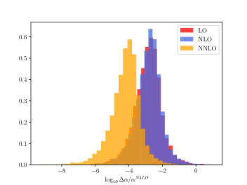
Figure 19: Distributions of the relative differences between $\alpha(0)_{\rm N4LO}$ and $\alpha(0)_{X}$, with $\rm X=LO,NLO,NNLO$. The $9000$ points considered were sampled over the space $q\in\ [0.1,1)$, $\theta_{1},\theta_{2}\in[0,\pi)$, and $\phi_{2}\in[0,2\pi)$. The median of the relative difference between the N4LO and LO or NLO distribution is $\Delta\alpha/\alpha\sim 10^{-3}$, about one order of magnitude larger than the difference between the NNLO and N4LO expressions. Given the analytical simplicity of the NLO expression, we decided to employ it for our current implementation for the $\alpha(0)$ computation.

At next-to-leading order (NLO), the $q\geq 1$ version of the orbital angular momentum and spin precession ODEs are given by Eqs. (11a, 11b) with the following initial conditions

$$\mathbf{S}_{1}(0) =m_{1}^{2}(\chi_{1x,0},\chi_{1y,0},\chi_{1z,0}),$$ (29)

$$\mathbf{S}_{2}(0) =m_{2}^{2}(\chi_{2x,0},\chi_{2y,0},\chi_{2z,0}),$$ (30)

$$\!\hat{\,\mathbf{L}}_{\text{N}}(0)=(0,0,1).$$ (31)

Recall the definition of $\alpha$:

$$\alpha=\arctan\left(\frac{\mathbf{L}_{\text{Ny}}}{\mathbf{L}_{\text{Nx}}}\right),$$ (32)

which is initially undefined as $\mathbf{L}_{\text{N}}$ points along the $z$ axis. However, as we explained in Sec. II, we mitigate this by using the initial torque instead as follows

$$\alpha(0)=\arctan\left(\frac{\dot{\hat{\,\mathbf{L}}}_{\text{N}}{}_{y}(0)}{\dot{\hat{\,\mathbf{L}}}_{\text{N}}{}_{x}(0)}\right),$$ (33)

where we employ the initial $x,y$ components of the $\dot{\hat{\,\mathbf{L}}}_{\text{N}}$ ODE. At NLO, this yields

$$\alpha(0)=\arctan\left(-\frac{q(3+4q)\chi_{1x,0}+(4+3q)\chi_{2x,0}}{q(3+4q)\chi_{1y,0}+(4+3q)\chi_{2y,0}}\right).$$ (34)

Eq. (33) can be straightforwardly extended to higher orders. Figure  19 shows the relative difference between $\alpha(0)$ computed at N4LO and lower orders.

Appendix B Numerical relativity data

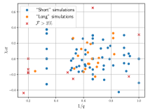
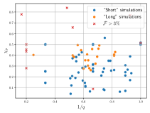
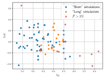
Figure 20: Properties of the two sets of NR data considered in Sec. III Buchman et al. (2012); Lovelace et al. (2008); Pfeiffer et al. (2007); Caudill et al. (2006); Cook and Pfeiffer (2004) to validate our EOB model. Different colors denote the two simulations sets employed. Crosses are used to indicate configurations for which the maximum EOB/NR unfaithfulness $\bar{\mathcal{F}}_{M}=\max_{M,\iota}\bar{\mathcal{F}}$ surpasses the $3\%$ threshold.

Figure 20 shows the properties of the two sets of NR data considered in this study Buchman et al. (2012); Lovelace et al. (2008); Pfeiffer et al. (2007); Caudill et al. (2006); Cook and Pfeiffer (2004) in terms of inverse mass ratio $m_{2}/m_{1}=1/q$, effective spin parameter $\chi_{\rm eff}$ and precessing spin parameter $\chi_{\rm p}$.

For the two sets consided, we have $q\in[1,6]$, $\chi_{p}\in[0.0424,0.7787]$ and $\chi_{\rm eff}\in[-0.4364,0.6522]$ (“short” simulations) and $q\in[1.217,4]$, $\chi_{p}\in[0.2616,0.4940]$, $\chi_{\rm eff}\in[-0.2276,0.3275]$ (“long” simulations).

References

- Abbott et al. (2016a) B. P. Abbott et al. (Virgo, LIGO Scientific), Phys. Rev. Lett. 116, 061102 (2016a), arXiv:1602.03837 [gr-qc] .
- Abbott et al. (2019a) B. P. Abbott et al. (LIGO Scientific, Virgo), Phys. Rev. X9, 011001 (2019a), arXiv:1805.11579 [gr-qc] .
- Abbott et al. (2018) B. P. Abbott et al. (LIGO Scientific, Virgo), Phys. Rev. Lett. 121, 161101 (2018), arXiv:1805.11581 [gr-qc] .
- Abbott et al. (2016b) B. P. Abbott et al. (Virgo, LIGO Scientific), Phys. Rev. Lett. 116, 241103 (2016b), arXiv:1606.04855 [gr-qc] .
- Abbott et al. (2017a) B. P. Abbott et al. (Virgo, LIGO Scientific), Astrophys. J. 851, L35 (2017a), arXiv:1711.05578 [astro-ph.HE] .
- Abbott et al. (2017b) B. P. Abbott et al. (Virgo, LIGO Scientific), Phys. Rev. Lett. 119, 141101 (2017b), arXiv:1709.09660 [gr-qc] .
- Abbott et al. (2017c) B. P. Abbott et al. (VIRGO, LIGO Scientific), Phys. Rev. Lett. 118, 221101 (2017c), arXiv:1706.01812 [gr-qc] .
- Abbott et al. (2019b) B. P. Abbott et al. (LIGO Scientific, Virgo), Phys. Rev. X9, 031040 (2019b), arXiv:1811.12907 [astro-ph.HE] .
- Venumadhav et al. (2019) T. Venumadhav, B. Zackay, J. Roulet, L. Dai, and M. Zaldarriaga, Phys. Rev. D 100, 023011 (2019), arXiv:1902.10341 [astro-ph.IM] .
- Venumadhav et al. (2020) T. Venumadhav, B. Zackay, J. Roulet, L. Dai, and M. Zaldarriaga, Phys. Rev. D 101, 083030 (2020), arXiv:1904.07214 [astro-ph.HE] .
- Nitz et al. (2019) A. H. Nitz, C. Capano, A. B. Nielsen, S. Reyes, R. White, D. A. Brown, and B. Krishnan, Astrophys. J. 872, 195 (2019), arXiv:1811.01921 [gr-qc] .
- Nitz et al. (2020) A. H. Nitz, T. Dent, G. S. Davies, S. Kumar, C. D. Capano, I. Harry, S. Mozzon, L. Nuttall, A. Lundgren, and M. Tápai, Astrophys. J. 891, 123 (2020), arXiv:1910.05331 [astro-ph.HE] .
- Abbott et al. (2020a) R. Abbott et al. (LIGO Scientific, Virgo), Astrophys. J. Lett. 896, L44 (2020a), arXiv:2006.12611 [astro-ph.HE] .
- Abbott et al. (2020b) R. Abbott et al. (LIGO Scientific, Virgo), Phys. Rev. D 102, 043015 (2020b), arXiv:2004.08342 [astro-ph.HE] .
- Abbott et al. (2020c) R. Abbott et al. (LIGO Scientific, Virgo), Phys. Rev. Lett. 125, 101102 (2020c), arXiv:2009.01075 [gr-qc] .
- Abbott et al. (2017d) B. P. Abbott et al. (Virgo, LIGO Scientific), Phys. Rev. Lett. 119, 161101 (2017d), arXiv:1710.05832 [gr-qc] .
- Abbott et al. (2020d) B. Abbott et al. (LIGO Scientific, Virgo), Astrophys. J. Lett. 892, L3 (2020d), arXiv:2001.01761 [astro-ph.HE] .
- Abbott et al. (2021a) R. Abbott et al. (LIGO Scientific, KAGRA, VIRGO), Astrophys. J. Lett. 915, L5 (2021a), arXiv:2106.15163 [astro-ph.HE] .
- Abbott et al. (2020e) R. Abbott et al. (LIGO Scientific, Virgo), Astrophys. J. Lett. 900, L13 (2020e), arXiv:2009.01190 [astro-ph.HE] .
- Bustillo et al. (2021) J. C. Bustillo, N. Sanchis-Gual, A. Torres-Forné, J. A. Font, A. Vajpeyi, R. Smith, C. Herdeiro, E. Radu, and S. H. W. Leong, Phys. Rev. Lett. 126, 081101 (2021), arXiv:2009.05376 [gr-qc] .
- Gayathri et al. (2020) V. Gayathri, J. Healy, J. Lange, B. O’Brien, M. Szczepanczyk, I. Bartos, M. Campanelli, S. Klimenko, C. Lousto, and R. O’Shaughnessy, (2020), arXiv:2009.05461 [astro-ph.HE] .
- Gamba et al. (2021a) R. Gamba, M. Breschi, G. Carullo, P. Rettegno, S. Albanesi, S. Bernuzzi, and A. Nagar, Submitted to Nature Astronomy (2021a), arXiv:2106.05575 [gr-qc] .
- Abbott et al. (2021b) R. Abbott et al. (LIGO Scientific, Virgo), Phys. Rev. X 11, 021053 (2021b), arXiv:2010.14527 [gr-qc] .
- Abbott et al. (2021c) R. Abbott et al. (LIGO Scientific, Virgo), Astrophys. J. Lett. 913, L7 (2021c), arXiv:2010.14533 [astro-ph.HE] .
- Apostolatos et al. (1994) T. A. Apostolatos, C. Cutler, G. J. Sussman, and K. S. Thorne, Phys. Rev. D49, 6274 (1994).
- Buonanno and Damour (1999) A. Buonanno and T. Damour, Phys. Rev. D59, 084006 (1999), arXiv:gr-qc/9811091 .
- Buonanno and Damour (2000) A. Buonanno and T. Damour, Phys. Rev. D62, 064015 (2000), arXiv:gr-qc/0001013 .
- Damour et al. (2000) T. Damour, P. Jaranowski, and G. Schaefer, Phys. Rev. D62, 084011 (2000), arXiv:gr-qc/0005034 [gr-qc] .
- Damour (2001) T. Damour, Phys. Rev. D64, 124013 (2001), arXiv:gr-qc/0103018 .
- Buonanno et al. (2006) A. Buonanno, Y. Chen, and T. Damour, Phys. Rev. D74, 104005 (2006), arXiv:gr-qc/0508067 .
- Damour et al. (2015) T. Damour, P. Jaranowski, and G. Schäfer, Phys. Rev. D91, 084024 (2015), arXiv:1502.07245 [gr-qc] .
- Damour and Nagar (2010) T. Damour and A. Nagar, Phys. Rev. D81, 084016 (2010), arXiv:0911.5041 [gr-qc] .
- Damour et al. (2012) T. Damour, A. Nagar, and L. Villain, Phys.Rev. D85, 123007 (2012), arXiv:1203.4352 [gr-qc] .
- Bernuzzi et al. (2012) S. Bernuzzi, A. Nagar, M. Thierfelder, and B. Brügmann, Phys.Rev. D86, 044030 (2012), arXiv:1205.3403 [gr-qc] .
- Bohé et al. (2017) A. Bohé et al., Phys. Rev. D95, 044028 (2017), arXiv:1611.03703 [gr-qc] .
- Babak et al. (2017) S. Babak, A. Taracchini, and A. Buonanno, Phys. Rev. D95, 024010 (2017), arXiv:1607.05661 [gr-qc] .
- Cotesta et al. (2018) R. Cotesta, A. Buonanno, A. Bohé, A. Taracchini, I. Hinder, and S. Ossokine, Phys. Rev. D98, 084028 (2018), arXiv:1803.10701 [gr-qc] .
- Hinderer et al. (2016) T. Hinderer et al., Phys. Rev. Lett. 116, 181101 (2016), arXiv:1602.00599 [gr-qc] .
- Steinhoff et al. (2016) J. Steinhoff, T. Hinderer, A. Buonanno, and A. Taracchini, Phys. Rev. D94, 104028 (2016), arXiv:1608.01907 [gr-qc] .
- Lackey et al. (2019) B. D. Lackey, M. Pürrer, A. Taracchini, and S. Marsat, Phys. Rev. D 100, 024002 (2019), arXiv:1812.08643 [gr-qc] .
- Matas et al. (2020) A. Matas et al., Phys. Rev. D 102, 043023 (2020), arXiv:2004.10001 [gr-qc] .
- Ossokine et al. (2020) S. Ossokine et al., Phys. Rev. D 102, 044055 (2020), arXiv:2004.09442 [gr-qc] .
- Damour and Nagar (2014a) T. Damour and A. Nagar, Phys.Rev. D90, 024054 (2014a), arXiv:1406.0401 [gr-qc] .
- Bernuzzi et al. (2015) S. Bernuzzi, A. Nagar, T. Dietrich, and T. Damour, Phys.Rev.Lett. 114, 161103 (2015), arXiv:1412.4553 [gr-qc] .
- Nagar et al. (2017) A. Nagar, G. Riemenschneider, and G. Pratten, Phys. Rev. D96, 084045 (2017), arXiv:1703.06814 [gr-qc] .
- Nagar et al. (2018) A. Nagar et al., Phys. Rev. D98, 104052 (2018), arXiv:1806.01772 [gr-qc] .
- Akcay et al. (2019) S. Akcay, S. Bernuzzi, F. Messina, A. Nagar, N. Ortiz, and P. Rettegno, Phys. Rev. D99, 044051 (2019), arXiv:1812.02744 [gr-qc] .
- Nagar et al. (2020) A. Nagar, G. Riemenschneider, G. Pratten, P. Rettegno, and F. Messina, Phys. Rev. D 102, 024077 (2020), arXiv:2001.09082 [gr-qc] .
- Rettegno et al. (2019) P. Rettegno, F. Martinetti, A. Nagar, D. Bini, G. Riemenschneider, and T. Damour, (2019), arXiv:1911.10818 [gr-qc] .
- Chiaramello and Nagar (2020) D. Chiaramello and A. Nagar, Phys. Rev. D 101, 101501 (2020), arXiv:2001.11736 [gr-qc] .
- Nagar et al. (2021a) A. Nagar, P. Rettegno, R. Gamba, and S. Bernuzzi, Phys. Rev. D 103, 064013 (2021a), arXiv:2009.12857 [gr-qc] .
- Albanesi et al. (2021) S. Albanesi, A. Nagar, and S. Bernuzzi, Phys. Rev. D 104, 024067 (2021), arXiv:2104.10559 [gr-qc] .
- Nagar et al. (2021b) A. Nagar, A. Bonino, and P. Rettegno, Phys. Rev. D 103, 104021 (2021b), arXiv:2101.08624 [gr-qc] .
- Nagar and Rettegno (2021) A. Nagar and P. Rettegno, (2021), arXiv:2108.02043 [gr-qc] .
- Ajith et al. (2007) P. Ajith, S. Babak, Y. Chen, M. Hewitson, B. Krishnan, et al., Class.Quant.Grav. 24, S689 (2007), arXiv:0704.3764 [gr-qc] .
- Ajith et al. (2008) P. Ajith, S. Babak, Y. Chen, M. Hewitson, B. Krishnan, et al., Phys.Rev. D77, 104017 (2008), arXiv:0710.2335 [gr-qc] .
- Ajith et al. (2011) P. Ajith, M. Hannam, S. Husa, Y. Chen, B. Brügmann, et al., Phys.Rev.Lett. 106, 241101 (2011), arXiv:0909.2867 [gr-qc] .
- Santamaria et al. (2010) L. Santamaria, F. Ohme, P. Ajith, B. Brügmann, N. Dorband, et al., Phys.Rev. D82, 064016 (2010), arXiv:1005.3306 [gr-qc] .
- Husa et al. (2016) S. Husa, S. Khan, M. Hannam, M. Pürrer, F. Ohme, X. Jiménez Forteza, and A. Bohé, Phys. Rev. D93, 044006 (2016), arXiv:1508.07250 [gr-qc] .
- Khan et al. (2016) S. Khan, S. Husa, M. Hannam, F. Ohme, M. Pürrer, X. Jiménez Forteza, and A. Bohé, Phys. Rev. D93, 044007 (2016), arXiv:1508.07253 [gr-qc] .
- Pratten et al. (2020) G. Pratten, S. Husa, C. Garcia-Quiros, M. Colleoni, A. Ramos-Buades, H. Estelles, and R. Jaume, Phys. Rev. D 102, 064001 (2020), arXiv:2001.11412 [gr-qc] .
- Estellés et al. (2021a) H. Estellés, A. Ramos-Buades, S. Husa, C. García-Quirós, M. Colleoni, L. Haegel, and R. Jaume, Phys. Rev. D 103, 124060 (2021a), arXiv:2004.08302 [gr-qc] .
- Estellés et al. (2020) H. Estellés, S. Husa, M. Colleoni, D. Keitel, M. Mateu-Lucena, C. García-Quirós, A. Ramos-Buades, and A. Borchers, (2020), arXiv:2012.11923 [gr-qc] .
- Estellés et al. (2021b) H. Estellés, M. Colleoni, C. García-Quirós, S. Husa, D. Keitel, M. Mateu-Lucena, M. d. L. Planas, and A. Ramos-Buades, (2021b), arXiv:2105.05872 [gr-qc] .
- Hamilton et al. (2021) E. Hamilton, L. London, J. E. Thompson, E. Fauchon-Jones, M. Hannam, C. Kalaghatgi, S. Khan, F. Pannarale, and A. Vano-Vinuales, (2021), arXiv:2107.08876 [gr-qc] .
- London et al. (2018) L. London, S. Khan, E. Fauchon-Jones, X. J. Forteza, M. Hannam, S. Husa, C. Kalaghatgi, F. Ohme, and F. Pannarale, Phys. Rev. Lett. 120, 161102 (2018), arXiv:1708.00404 [gr-qc] .
- García-Quirós et al. (2020) C. García-Quirós, M. Colleoni, S. Husa, H. Estellés, G. Pratten, A. Ramos-Buades, M. Mateu-Lucena, and R. Jaume, Phys. Rev. D 102, 064002 (2020), arXiv:2001.10914 [gr-qc] .
- Khan et al. (2019a) S. Khan, F. Ohme, K. Chatziioannou, and M. Hannam, (2019a), arXiv:1911.06050 [gr-qc] .
- Hannam et al. (2014) M. Hannam, P. Schmidt, A. Bohé, L. Haegel, S. Husa, F. Ohme, G. Pratten, and M. Pürrer, Phys. Rev. Lett. 113, 151101 (2014), arXiv:1308.3271 [gr-qc] .
- Schmidt et al. (2015) P. Schmidt, F. Ohme, and M. Hannam, Phys. Rev. D91, 024043 (2015), arXiv:1408.1810 [gr-qc] .
- Khan et al. (2019b) S. Khan, K. Chatziioannou, M. Hannam, and F. Ohme, Phys. Rev. D100, 024059 (2019b), arXiv:1809.10113 [gr-qc] .
- Pratten et al. (2021) G. Pratten et al., Phys. Rev. D 103, 104056 (2021), arXiv:2004.06503 [gr-qc] .
- Dietrich et al. (2017) T. Dietrich, S. Bernuzzi, and W. Tichy, Phys. Rev. D96, 121501 (2017), arXiv:1706.02969 [gr-qc] .
- Dietrich et al. (2019) T. Dietrich, A. Samajdar, S. Khan, N. K. Johnson-McDaniel, R. Dudi, and W. Tichy, Phys. Rev. D100, 044003 (2019), arXiv:1905.06011 [gr-qc] .
- Blackman et al. (2014) J. Blackman, B. Szilagyi, C. R. Galley, and M. Tiglio, Phys. Rev. Lett. 113, 021101 (2014), arXiv:1401.7038 [gr-qc] .
- Blackman et al. (2017) J. Blackman, S. E. Field, M. A. Scheel, C. R. Galley, D. A. Hemberger, P. Schmidt, and R. Smith, Phys. Rev. D95, 104023 (2017), arXiv:1701.00550 [gr-qc] .
- Varma et al. (2019a) V. Varma, S. E. Field, M. A. Scheel, J. Blackman, L. E. Kidder, and H. P. Pfeiffer, Phys. Rev. D99, 064045 (2019a), arXiv:1812.07865 [gr-qc] .
- Varma et al. (2019b) V. Varma, S. E. Field, M. A. Scheel, J. Blackman, D. Gerosa, L. C. Stein, L. E. Kidder, and H. P. Pfeiffer, Phys. Rev. Research. 1, 033015 (2019b), arXiv:1905.09300 [gr-qc] .
- Williams et al. (2019) D. Williams, I. S. Heng, J. Gair, J. A. Clark, and B. Khamesra, (2019), arXiv:1903.09204 [gr-qc] .
- Akcay et al. (2021) S. Akcay, R. Gamba, and S. Bernuzzi, Phys. Rev. D 103, 024014 (2021), arXiv:2005.05338 [gr-qc] .
- Gamba et al. (2021b) R. Gamba, M. Breschi, S. Bernuzzi, M. Agathos, and A. Nagar, Phys. Rev. D 103, 124015 (2021b), arXiv:2009.08467 [gr-qc] .
- (82) “SXS Gravitational Waveform Database,” https://data.black-holes.org/waveforms/index.html.
- Ajith (2011) P. Ajith, Phys.Rev. D84, 084037 (2011), arXiv:1107.1267 [gr-qc] .
- Racine (2008) E. Racine, Phys. Rev. D78, 044021 (2008), arXiv:0803.1820 [gr-qc] .
- Schmidt et al. (2011) P. Schmidt, M. Hannam, S. Husa, and P. Ajith, Phys. Rev. D84, 024046 (2011), arXiv:1012.2879 [gr-qc] .
- Schmidt et al. (2012) P. Schmidt, M. Hannam, and S. Husa, Phys. Rev. D86, 104063 (2012), arXiv:1207.3088 [gr-qc] .
- Boyle et al. (2011) M. Boyle, R. Owen, and H. P. Pfeiffer, Phys. Rev. D84, 124011 (2011), arXiv:1110.2965 [gr-qc] .
- O’Shaughnessy et al. (2011) R. O’Shaughnessy, B. Vaishnav, J. Healy, Z. Meeks, and D. Shoemaker, Phys. Rev. D84, 124002 (2011), arXiv:1109.5224 [gr-qc] .
- Pan et al. (2014a) Y. Pan, A. Buonanno, A. Taracchini, L. E. Kidder, A. H. Mroue, et al., Phys.Rev. D89, 084006 (2014a), arXiv:1307.6232 [gr-qc] .
- Nagar et al. (2019a) A. Nagar, G. Pratten, G. Riemenschneider, and R. Gamba, (2019a), arXiv:1904.09550 [gr-qc] .
- Damour and Nagar (2014b) T. Damour and A. Nagar, Phys.Rev. D90, 044018 (2014b), arXiv:1406.6913 [gr-qc] .
- Damour et al. (2008) T. Damour, P. Jaranowski, and G. Schäfer, Phys.Rev. D78, 024009 (2008), arXiv:0803.0915 [gr-qc] .
- Nagar et al. (2019b) A. Nagar, F. Messina, P. Rettegno, D. Bini, T. Damour, A. Geralico, S. Akcay, and S. Bernuzzi, Phys. Rev. D99, 044007 (2019b), arXiv:1812.07923 [gr-qc] .
- Bini et al. (2012) D. Bini, T. Damour, and G. Faye, Phys.Rev. D85, 124034 (2012), arXiv:1202.3565 [gr-qc] .
- Bini and Damour (2014) D. Bini and T. Damour, Phys.Rev. D90, 124037 (2014), arXiv:1409.6933 [gr-qc] .
- Nagar (2011) A. Nagar, Phys.Rev. D84, 084028 (2011), arXiv:1106.4349 [gr-qc] .
- Buonanno et al. (2003) A. Buonanno, Y.-b. Chen, and M. Vallisneri, Phys. Rev. D67, 104025 (2003), [Erratum: Phys. Rev.D74,029904(2006)], arXiv:gr-qc/0211087 [gr-qc] .
- Buonanno et al. (2009) A. Buonanno, B. Iyer, E. Ochsner, Y. Pan, and B. Sathyaprakash, Phys.Rev. D80, 084043 (2009), arXiv:0907.0700 [gr-qc] .
- Chatziioannou et al. (2013) K. Chatziioannou, A. Klein, N. Yunes, and N. Cornish, Phys. Rev. D88, 063011 (2013), arXiv:1307.4418 [gr-qc] .
- Pan et al. (2014b) Y. Pan, A. Buonanno, A. Taracchini, M. Boyle, L. E. Kidder, et al., Phys.Rev. D89, 061501 (2014b), arXiv:1311.2565 [gr-qc] .
- Nagar and Rettegno (2019) A. Nagar and P. Rettegno, Phys. Rev. D99, 021501 (2019), arXiv:1805.03891 [gr-qc] .
- Jiménez-Forteza et al. (2017) X. Jiménez-Forteza, D. Keitel, S. Husa, M. Hannam, S. Khan, and M. Pürrer, Phys. Rev. D95, 064024 (2017), arXiv:1611.00332 [gr-qc] .
- Varma et al. (2019c) V. Varma, D. Gerosa, L. C. Stein, F. Hébert, and H. Zhang, Phys. Rev. Lett. 122, 011101 (2019c), arXiv:1809.09125 [gr-qc] .
- O’Shaughnessy et al. (2013) R. O’Shaughnessy, L. London, J. Healy, and D. Shoemaker, Phys. Rev. D 87, 044038 (2013), arXiv:1209.3712 [gr-qc] .
- Berti et al. (2006) E. Berti, V. Cardoso, and C. M. Will, Phys. Rev. D73, 064030 (2006), arXiv:gr-qc/0512160 .
- Ramos-Buades et al. (2020) A. Ramos-Buades, P. Schmidt, G. Pratten, and S. Husa, Phys. Rev. D 101, 103014 (2020), arXiv:2001.10936 [gr-qc] .
- Gamba et al. (2021c) R. Gamba, S. Bernuzzi, and A. Nagar, Phys. Rev. D 104, 084058 (2021c), arXiv:2012.00027 [gr-qc] .
- Zackay et al. (2018) B. Zackay, L. Dai, and T. Venumadhav, (2018), arXiv:1806.08792 [astro-ph.IM] .
- Vinciguerra et al. (2017) S. Vinciguerra, J. Veitch, and I. Mandel, Class. Quant. Grav. 34, 115006 (2017), arXiv:1703.02062 [gr-qc] .
- Harry et al. (2016) I. Harry, S. Privitera, A. Bohé, and A. Buonanno, Phys. Rev. D94, 024012 (2016), arXiv:1603.02444 [gr-qc] .
- (111) “SXS collaboration catalog tools,” https://github.com/sxs-collaboration/catalog_tools.
- Schmidt et al. (2017) P. Schmidt, I. W. Harry, and H. P. Pfeiffer, (2017), arXiv:1703.01076 [gr-qc] .
- (113) “Updated Advanced LIGO sensitivity design curve,” https://dcc.ligo.org/LIGO-T1800044/public.
- Breschi et al. (2021) M. Breschi, R. Gamba, and S. Bernuzzi, Phys. Rev. D 104, 042001 (2021), arXiv:2102.00017 [gr-qc] .
- Godzieba and Radice (2021) D. A. Godzieba and D. Radice, Universe 7, 368 (2021), arXiv:2109.01159 [astro-ph.HE] .
- Speagle (2020) J. S. Speagle, Monthly Notices of the Royal Astronomical Society 493, 3132?3158 (2020).
- Abbott et al. (2016c) B. P. Abbott et al. (Virgo, LIGO Scientific), Phys. Rev. Lett. 116, 241102 (2016c), arXiv:1602.03840 [gr-qc] .
- Islam et al. (2021) T. Islam, S. E. Field, C.-J. Haster, and R. Smith, Phys. Rev. D 103, 104027 (2021), arXiv:2010.04848 [gr-qc] .
- Colleoni et al. (2021) M. Colleoni, M. Mateu-Lucena, H. Estellés, C. García-Quirós, D. Keitel, G. Pratten, A. Ramos-Buades, and S. Husa, Phys. Rev. D 103, 024029 (2021), arXiv:2010.05830 [gr-qc] .
- Hessels et al. (2006) J. W. T. Hessels, S. M. Ransom, I. H. Stairs, P. C. C. Freire, V. M. Kaspi, and F. Camilo, Science 311, 1901 (2006), arXiv:astro-ph/0601337 [astro-ph] .
- Kramer and Wex (2009) M. Kramer and N. Wex, Class. Quant. Grav. 26, 073001 (2009).
- Stovall et al. (2018) K. Stovall et al., Astrophys. J. 854, L22 (2018), arXiv:1802.01707 [astro-ph.HE] .
- Wade et al. (2014) L. Wade, J. D. E. Creighton, E. Ochsner, B. D. Lackey, B. F. Farr, T. B. Littenberg, and V. Raymond, Phys. Rev. D89, 103012 (2014), arXiv:1402.5156 [gr-qc] .
- Buchman et al. (2012) L. T. Buchman, H. P. Pfeiffer, M. A. Scheel, and B. Szilagyi, Phys. Rev. D86, 084033 (2012), arXiv:1206.3015 [gr-qc] .
- Lovelace et al. (2008) G. Lovelace, R. Owen, H. P. Pfeiffer, and T. Chu, Phys. Rev. D 78, 084017 (2008), arXiv:0805.4192 [gr-qc] .
- Pfeiffer et al. (2007) H. P. Pfeiffer, D. A. Brown, L. E. Kidder, L. Lindblom, G. Lovelace, and M. A. Scheel, New frontiers in numerical relativity. Proceedings, International Meeting, NFNR 2006, Potsdam, Germany, July 17-21, 2006, Class. Quant. Grav. 24, S59 (2007), arXiv:gr-qc/0702106 [gr-qc] .
- Caudill et al. (2006) M. Caudill, G. B. Cook, J. D. Grigsby, and H. P. Pfeiffer, Phys. Rev. D 74, 064011 (2006), arXiv:gr-qc/0605053 .
- Cook and Pfeiffer (2004) G. B. Cook and H. P. Pfeiffer, Phys. Rev. D70, 104016 (2004), arXiv:gr-qc/0407078 [gr-qc] .