bajes: Bayesian inference of multimessenger astrophysical data
Methods and application to gravitational-waves

Abstract

We present bajes, a parallel and lightweight framework for Bayesian inference of multimessenger transients. bajes is a Python modular package with minimal dependencies on external libraries adaptable to the majority of the Bayesian models and to various sampling methods. We describe the general workflow and the parameter estimation pipeline for compact-binary-coalescence gravitational-wave transients. The latter is validated against injections of binary black hole and binary neutron star waveforms, including confidence interval tests that demonstrates the inference is well-calibrated. Binary neutron star postmerger injections are also studied using a network of five detectors made of LIGO, Virgo, KAGRA and Einstein Telescope. Postmerger signals will be detectable for sources at ${\lesssim}80\,$Mpc, with Einstein Telescope contributing over 90% of the total signal-to-noise ratio. As a full scale application, we re-analyze the GWTC-1 black hole transients using the effective-one-body TEOBResumS approximant, and reproduce selected results with other approximants. bajes inferences are consistent with previous results; the direct comparison of bajes and bilby analyses of GW150914 shows a maximum Jensen-Shannon divergence of $5.2{\times}10^{-4}$. GW170817 is re-analyzed using TaylorF2 with 5.5PN point-mass and 7.5PN tides, TEOBResumSPA, and IMRPhenomPv2_NRTidal with different cutoff-frequencies of $1024\,$Hz and $2048\,$Hz. We find that the former choice minimizes systematics on the reduced tidal parameter, while a larger amount of tidal information is gained with the latter choice. bajes can perform these analyses in about 1 day using 128 CPUs.

I Introduction

Bayesian inference has become a standard method for the analysis of astrophysical and cosmological events, e.g. Abbott et al. (2019a); Del Pozzo et al. (2018); Wang (2019); Abbott et al. (2020a); Hortúa et al. (2020), since it offers a generic statistical framework to rigorously test hypothesis against observational information. Given a set of parametric models (hypothesis) and assumptions on the parameters (prior), Bayesian inference allows one to infer the parameters in terms of probability distributions, and also to select the best-fitting model among competing hypotheses. In particular, Bayesian methods are central tools used in gravitational-wave (GW) astronomy to determine the source properties of an observed signal Veitch and Vecchio (2010); Veitch et al. (2015); Abbott et al. (2020b) and the related applications. Some examples are tests of General Relativity Abbott et al. (2019b); Breschi et al. (2019a), astrophysical population studies Abbott et al. (2020c), inferences of the neutron star matter properties Abbott et al. (2018a) and cosmology Abbott et al. (2017a, 2019c). Furthermore, Bayesian inference offers the optimal framework to combine different observational datasets from multimessenger astronomical observations, like GW170817 and the electromagnetic (EM) counterparts Abbott et al. (2017b, c); Savchenko et al. (2017); Pian et al. (2017); Smartt et al. (2017); Tanvir et al. (2017); Tanaka et al. (2017); Villar et al. (2017). Multimessenger inference of astrophysical phenomena such as binary neutron star mergers (BNS) is a fundamental resource to clarify the mechanism at the origin of the radiation, to obtain accurate inferences on the properties of the source, and to improve theoretical models gaining information from observational data (e.g. Radice and Dai, 2019; Dietrich et al., 2020; Breschi et al., 2021a).

In the last years, many efforts have been made by the scientific community in the development of sophisticated parameter inference tools for astronomical observations. In the context of GW data analysis, LALSuite LIGO Scientific Collaboration (2018a) is the official software provided by the LIGO-Virgo collaboration Aasi et al. (2015); Acernese et al. (2015) and it offers a variegated framework for generic analysis of GW data. Other mature software for parameter estimation of GW transients are also available; some example are the semi-analytical integrator RIFT Pankow et al. (2015); Lange et al. (2018), the user-friendly library bilby Ashton et al. (2019) and the inference module of the pycbc package Biwer et al. (2019). Bayesian software for parameter inference of other astrophysical transients have also been developed, such as tools for high-energy photons from compact objects and galaxy clusters  Nasa High Energy Astrophysics Science Archive Research Center (2014) (Heasarc); Center ; Olamaie et al. (2015); neutrino radiation Aartsen et al. (2020); supernovae transients Shariff et al. (2016); Hinton et al. (2019); Möller and de Boissière (2019); pulsar arrival timings Edwards et al. (2006); Lentati et al. (2013); Luo et al. (2021); and for cosmological inferences Lewis and Bridle (2002); Das and Souradeep (2014); Ishida et al. (2015); Handley et al. (2015). Current pipelines for the analysis of astrophysical and cosmological observations are targeted to specific applications. However, within a multi-messenger framework, it is essential to develop a flexible pipeline capable of combining different datasets and physical models. This issue can be tackled allowing the infrastructure to merge different Bayesian models, extending the considered parameter space and generalizing the definition of the likelihood function. This implies the use of large amounts of data and computationally expensive models. It follows that efficient parallelization techniques and well-calibrated proposal methods are necessary to optimize the performances of such a flexible pipeline.

In this work, we present bajes [baIEs], a Python package for Bayesian inference developed at Friedrich-Schiller-Universtät Jena. Our goal is to provide a simple, complete and reliable implementation capable to robustly perform Bayesian inference on arbitrary sets of data, with specific functionalities for multimessenger astrophysics. The software is designed to be state-of-art, simple-to-use and light-weighted with minimal dependencies on external libraries. The paper is structured as follows. In Sec. II, we recall the basic concepts of Bayesian theory of probability. In Sec. III, we describe the design and the workflow of the bajes software. Sec. IV describes the tools and the methods implemented in bajes for the analysis of GW transients, including the available templates. In Sec. V, we describe the GW pipeline and the Bayesian framework of the GW model. In Sec. VI, we present a survey of injection studies and validation tests performed with artificial binary merger signals. Sec. VII shows the results of the bajes pipeline on the GW events observed by the LIGO-Virgo interferometers Abbott et al. (2019a, d). Finally, we conclude in Sec. VIII. The paper concludes with Appendices on the implemented sampling methods, the proposal methods and a simple use example.

II Bayesian inference

The task of a Bayesian inference is the formulation and the computation of conditional probabilities. It is possible to classify this topic in two main problems: parameter estimation (PE) and model selection (MS). With PE we mean the evaluation of the characteristic distribution for the parameters that define the model of interest. On the other hand, with MS we refer to the discrimination between competing models in light of the data, comparing the suitability of different assumptions directly on the observation. In order to discuss how these tasks are achieved, in the following sections we recall the basic concepts of Bayesian theory of probability. By convention, we label the natural logarithm as $\log$ throughout all the paper.

II.1 Bayes' theorem

Given a set of observed data d and a set of parameters $\bm{\theta}$, that characterizes our model within some background hypothesis $H$, it is possible to estimate the posterior distribution for $\bm{\theta}$ using the Bayes' theorem MacKay (2002); Gelman et al. (2004); Sivia and Skilling (2006),

$$p(\bm{\theta}|\textbf{d},H)=\frac{p(\textbf{d}|\bm{\theta},H)\,p(\bm{\theta}|H)}{p(\textbf{d}|H)}\,,$$ (1)

where $p(\textbf{d}|\bm{\theta},H)$ is the likelihood function, $p(\bm{\theta}|H)$ is the prior distribution and $p(\textbf{d}|H)$ is the evidence. The likelihood function describes the probability of observing the data d given $\bm{\theta}$ and assuming that the hypothesis $H$ is true. Therefore, it encodes the observational information and it predicts the agreement between the observed data d and the expected outcome for every given sample $\bm{\theta}$ of the parameter space. The prior distribution $p(\bm{\theta}|H)$ depicts the knowledge on the parameters before performing the estimation. Usually, the functional form of this term is chosen in accordance with geometrical and/or physically-motivated argumentation. The term $p(\textbf{d}|H)$ is labeled as evidence and it represents the probability of observing the data d given the hypothesis $H$. The evidence is also called marginalized likelihood since, according to the marginalization rule, it can be expressed as

$$p(\textbf{d}|H)=\int_{\bm{\Theta}}p(\textbf{d}|\bm{\theta},H)\,p(\bm{\theta}|H)\,\text{d}\bm{\theta}\,,$$ (2)

where the integral is extended over the entire parameter space $\bm{\Theta}$. Subsequently, the posterior distribution $p(\bm{\theta}|\textbf{d},H)$ represents the probability of the parameters $\bm{\theta}$ in light of the data overhauled by our a priori information. The knowledge of $p(\bm{\theta}|\textbf{d},H)$ allows us to compute the expectation of the statistical quantities of interest. For example, the mean values $E[\bm{\theta}]$ can be estimated as

$$E[\bm{\theta}]=\int_{\bm{\Theta}}\bm{\theta}\,p(\bm{\theta}|\textbf{d},H)\,\text{d}\bm{\theta}\,,$$ (3)

and, analogously, it is possible to infer the expectation of a generic function of the parameters $\bm{\theta}$,

$$E\left[f(\bm{\theta})\right]=\int_{\bm{\Theta}}f(\bm{\theta})\,p(\bm{\theta}|\textbf{d},H)\,\text{d}\bm{\theta}\,.$$ (4)

From this argumentation it follows that, in order to perform PE, we have to introduce a prior distribution $p(\bm{\theta}|H)$ and a likelihood function $p(\textbf{d}|\bm{\theta},H)$; then, the properties of the model are encoded in the posterior distribution $p(\bm{\theta}|\textbf{d},H)$ that can be computed imposing Eq. (1).

II.2 Model selection

In Eq. (1), for a fixed set of assumptions $H$, the evidence acts like a normalization constant; however, this quantity plays a crucial role in the context of MS. If we are interested in comparing two competing hypotheses, $H_{A}$ and $H_{B}$, quantifying which one is better explaining the data, in the Bayesian framework it is natural to introduce the odds ratio,

$$\mathcal{O}_{A}^{B}=\frac{p(H_{B}|\textbf{d})}{p(H_{A}|\textbf{d})}=\frac{p(H_{B})}{p(H_{A})}\,\frac{p(\textbf{d}|H_{B})}{p(\textbf{d}|H_{A})}\,.$$ (5)

The term $p(H_{i}|\textbf{d})$ represents the posterior probability for the $i$-th hypothesis given the observed data and the ratio $\mathcal{O}_{A}^{B}$ encodes the will of the data in favoring one model over another. Assuming that the two hypotheses are equiprobable $p(H_{B})=p(H_{A})$, it is possible to reduce the computation to the ratio of the evidences, also known as Bayes' factor,

$$\mathcal{B}_{A}^{B}=\frac{p(\textbf{d}|H_{B})}{p(\textbf{d}|H_{A})}\,.$$ (6)

If $\mathcal{B}_{A}^{B}<1$ then the hypothesis $A$ is preferred by the data, otherwise $B$ is favored if $\mathcal{B}_{A}^{B}>1$. However, this rule is not always straightforward since the estimation of the Bayes' factor might suffer of uncertainties Mattei (2020); Yao et al. (2019). Then, in a realistic scenario, more stringent bounds are required in order to prefer a hypothesis Kass and Raftery (1995).

II.3 Joint distributions

Let us assume that we performed two independent observations, $\textbf{d}_{1}$ and $\textbf{d}_{2}$, and each of them can be modeled using two sets of parameters, respectively $\bm{\theta}_{1}$ and $\bm{\theta}_{2}$. In general, it is possible to apply Bayes' theorem, Eq. (1), separately to every set of measurements. However, if the two events are not independent (e.g. the same physical process observed by two different observatories), the joint posterior distribution can be written as

$$p(\bm{\theta}_{1},\bm{\theta}_{2}|\textbf{d}_{1},\textbf{d}_{2},H)=\frac{p(\textbf{d}_{1},\textbf{d}_{2}|\bm{\theta}_{1},\bm{\theta}_{2},H)\,p(\bm{\theta}_{1},\bm{\theta}_{2}|H)}{p(\textbf{d}_{1},\textbf{d}_{2}|H)}\,,$$ (7)

where $p(\textbf{d}_{1},\textbf{d}_{2}|\bm{\theta}_{1},\bm{\theta}_{2},H)$ is the joint likelihood function and $p(\bm{\theta}_{1},\bm{\theta}_{2}|H)$ is the joint prior distribution. If the employed set of parameters $\bm{\theta}_{1}$ and $\bm{\theta}_{2}$ are independent, the joint probabilities simply correspond to the product of the single probability terms. However, if $\bm{\theta}_{1}$ and $\bm{\theta}_{2}$ correlate, the problem could easily become non-trivial; e.g. the intersection between the two parameter spaces $\bm{\Theta}_{1}\cap\bm{\Theta}_{2}$ could be not empty, or the value of the two sets of parameters could be related with each other $\bm{\theta}_{i}\equiv\bm{\theta}_{i}(\bm{\theta}_{j})$, or unexpected correlations might appear introducing a larger parameter space.

II.4 Samplers

In a realistic scenario, the form of the likelihood function is not always analytically determinable and the parameter space has usually a large number of dimensions. For these reasons, the evaluation of the posterior distribution and the estimation of its integral are performed with stochastic techniques. In particular, sampling methods have proven to be reliable and generic tools for the analysis of non-analytical forms and multi-dimensional parameter spaces Allison and Dunkley (2013); Veitch et al. (2015); Tichy (2015); Handley et al. (2015), capable to give robust and stable results.

Markov-chain Monte Carlo (MCMC) methods are suitable tools to perform PE, exploring the parameter space through random-walks and collecting samples along the evolution. Subsequently, the posterior distribution is estimated using the set of independent samples of the parameter space. Nevertheless, the nested sampling Skilling (2006) is an advanced algorithm capable to extract posterior samples and perform accurate estimation of the evidence, which is the key quantity for MS. In order to solve this task, each sample is assumed to be the representative of a isoprobability contour. Then, the evidence is computed as the sum of the likelihood values weighted on the respective prior volume, estimated resorting to Bayesian calculations. The details of the sampling methods are discussed in App. A and App. B.

III Design of the code

bajes is a pure Python software that aims to provide a versatile and robust framework for generic Bayesian inference within a simple and clear approach. In order to achieve this task, the software relies on a modular and composed architecture and it implements logically specialized objects. Furthermore, we decide to keep a light-weight setup with minimal dependencies on external libraries. These properties make bajes a simple and general tool with a wide range of applicability. The body of the bajes software is constituted by two components: the inf module, that represents an implementation of the Bayesian logic, and the obs module, that contains the tools to manage and process physical data.

The inf module is the Bayesian skeleton of the software and contains the methods required to instantiate the model to be inferred. Sec. III.1 describes the tools implemented in bajes.inf and the general workflow of the module. The Bayesian approach is constituted by three fundamental stages Gelman (2008): formulating a model, comparing the model with the data and inferring the properties of the model. The goal of the inf module is to provide a flexible and general interface capable to adapt itself to a broad variety of problems. This structure promotes usability and applicability, supplying a comprehensive and unique architecture that allows the user to tackle specific problems. In order to enforce these concepts, the software is developed promoting an intuitive manageability and the simplicity of use: providing the necessary basic information, the user can easily set up a full Bayesian analysis. App. D shows an example of a practical PE analysis with bajes tools.

In the context of data analysis, the statistical infrastructure has to be flanked by the physical characterization of the experimental data with the purpose of defining a full Bayesian model. This is necessary in order to connect the statistical properties with the actual observable quantities. Obviously, the specific physical model to be used depends on the nature of the analyzed data, on the assumptions made to build the model, and, in general, different physical events will require tailored treatments and specialized tools. To address this, bajes provides the obs module, which is a container of methods needed to characterize and handle specific physical observations. This module is designed aiming to the analysis of GWs and EM counterparts. Currently, bajes.obs includes two sub-modules: gw and kn. The gw module contains the tools necessary to deal with GW analysis and it is described in Sec. IV. The kn module supplies a framework for the analysis of kilonovae light curves generated by BNS collisions, following our early work Breschi et al. (2021a). The implementation of the kn module is inspired by the approach presented in Ref. Perego et al. (2017); Breschi et al. (2021a) and it will be detailed in a followup work.

III.1 Workflow

Figure 1: Schematic representation of the workflow described in Sec. III.1. The scheme highlights the three stages of the Bayesian formalism: formulation of the model, fitting the model to the data and inference of the model properties. The gray box constituted by likelihood function and prior assumptions represents the Bayesian model to be inferred. The dashed back-propagating line refer to the case in which the analysis is iterated with an improved description.

In order to fulfill the generic tasks of Bayesian inference, bajes provides the tools necessary to instantiate a Bayesian model Gelman et al. (2020) and to extract the statistical quantities of interest, such as posterior distribution or evidence.

The bajes.inf module supplies a Prior and a Likelihood objects, and their combination defines the Bayesian model. The Prior provides the implementation of a generic prior distribution: this object can be instantiated with list of Parameter, that are going to define the parameter space of the model. It is also possible to introduce constant and variable quantities to be carried along the sampling. Subsequently, it is possible to introduce a likelihood function customizing the specific log_like method of a Likelihood object. Furthermore, bajes implements a JointPrior and a JointLikelihood objects in order to handle joint posterior distributions. Additionally, planned extensions include hierarchical models (e.g. Hinton et al., 2019; Loredo and Hendry, 2019) and Bayesian methods to deal with error propagation.

Once the Bayesian model is defined, it is possible to fit the model to the data estimating its properties. The inf module provides a Sampler method that wraps the provided model and initializes the requested sampling algorithm. As mentioned in Sec. II.4, the sampler explores the parameter space aiming to reconstruct the posterior distribution. In order to conduct an accurate analysis, the Sampler objects rely on auxiliary functions such as the proposal methods described in App. C: these are statistical techniques that aim to extract independent samples and to conduct the sampler towards more likely regions of the parameter space. (see App. A and App. B).

When the Sampler completes the analysis, the algorithm returns the conditioned probability of interest and the properties of the model can be inferred. This information allows us to to compute the statistical quantities that characterize the model and make it possible to test competing hypotheses and verify different assumptions. Moreover, from these results it is possible to understand the limits of the involved description; then, in general, the model can be improved and the workflow can be iterated with the reviewed model, improving the understanding and the modeling of the observed event. Figure 1 shows a schematic representation of the described workflow.

III.2 Parallelisation

Figure 2: Scaling plot for the bajes pipeline (see Sec. V). Top panel: The square markers are the measured speedup factors with respect to the serial execution-time. The execution-times for the PTMCMC (orange squares) algorithm are estimated performing $10^{3}$ iterations with $128\times 4$ tempered chains. The nested sampling execution-times (pink squares for multi-threading and green squares for MPI) are computed employing the dynesty software with 1024 live points and tolerance equal to 0.1. The blue solid line is the ideal linear scaling and the yellow solid line is the theoretical scaling of nested sampling. Bottom panel: Same quantities discussed in the previous panel expressed in terms of efficiency.

By default, bajes analyses can be performed taking advantage of the parallel-threading multiprocess Python library. However, with this method the number of available processes is strictly limited by the size of the single machine and for non-trivial problems this could be a strong limitation. For this reason, the bajes software implements a customized method for multi-nodes communication based on the message passing interface (MPI) protocol.

For ideal scaling, the execution-time of a machine computation is inversely proportional to the number of central processing units (CPUs), that leads to a linearly increase of the speedup. However, in a realistic scenario, the scaling performances of sampling techniques are affected by unavoidable computational steps serially performed (e.g. temperature swapping in parallel chains and live points collection of nested sampling) and by the continuous exchange of information between different processes, required to adapt the evolution of the algorithm.

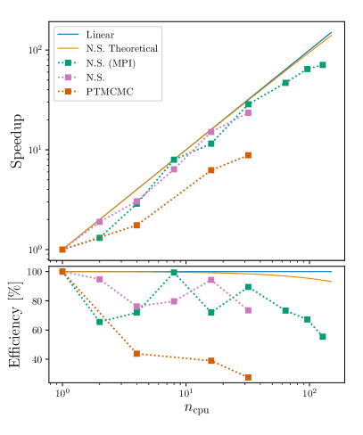
MCMC and nested sampling algorithms require separate treatments. The performances of MCMC sampling are typically quantified in terms of proposal acceptance and correlation length of the chains Patil et al. (2010); Solonen et al. (2012); Foreman-Mackey et al. (2013); Veitch et al. (2015); Li and Marzouk (2014); Vousden et al. (2015), and generally the overall execution-time is determined by several contributions, such as the total number of chains, the complexity of the parameter space and the employed proposal techniques. Estimations of MCMC execution-times Šukys and Kattwinkel (2017); Robert et al. (2018); Morzfeld et al. (2019) have shown that the efficiency drastically decreases for an increasing number of parallel chains. On the other hand, the parallelization performances of the nested sampling are well studied Feroz and Hobson (2008); Handley et al. (2015); Brewer and Foreman-Mackey (2016); Higson et al. (2018); Smith et al. (2020) and the theoretical speedup factor $S_{\rm NS}$ of this algorithm is expressed as a sub-linear scaling,

$$S_{\rm NS}(n_{\rm live},n_{\rm cpu})=n_{\rm live}\cdot\log\left(1+\frac{n_{\rm cpu}}{n_{\rm live}}\right)\,.$$ (8)

For $n_{\rm live}\gg n_{\rm cpu}$, the values predicted by Eq. (8) are comparable with a linear trend.

Figure 2 shows the measured speedup factors in the execution-time as a function of the number of CPUs for different samplers and different parallelization methods. The speedup factors are computed with respect to the execution-time measured from the serial job. The execution-times are estimated from the bajes GW pipeline (see Sec. V) using GW150914 Abbott et al. (2016a) as target signal (see Sec. VII.1). Moreover, Figure 2 shows the respective efficiency rates, that encode the deviation from the ideal linear scaling. The efficiency is computed as the percentage ratio between the measure speedup factor and the number of employed CPUs. Ideal linear scaling has an efficiency of 100%.

For the parallel-tempered MCMC (PTMCMC) algorithm implemented in bajes, we estimate the speedup performing $10^{3}$ iterations with $128\times 4$ tempered chains, while, for nested sampling, we employ the dynesty software with 1024 live points and tolerance equal to 0.1. The PTMCMC is not optimal in terms of execution-time scaling, mainly due to the serial swapping routine. However, it gives acceptable scaling performances with efficiency $\gtrsim 40\%$ up to $n_{\rm cpu}\simeq 16$ using multi-threading methods. The results with MPI are worst compared to multi-threading due to the data communication.

Regarding the nested sampling, for a very small number of processes, roughly $n_{\rm cpu}\lesssim 2$, the multi-threading method gives more efficient results, since the MPI protocol requires additional time for data communication. For an increasing number of CPUs, roughly $n_{\rm cpu}\gtrsim 6$, the two parallelization methods give comparable results. However, the strength of MPI parallelization is the capability of accessing multiple CPUs located in different physical machines: the MPI interface implemented in bajes gives an efficiency greater than 70% up to $n_{\rm cpu}\simeq 100$, that is the typical size of standard PE job.

III.3 Dependencies

The bajes software is compatible with Python 3.7 or higher versions, and it can be easily installed using the standard Python setup tools. It relies on essential modules, preferring those that can be easily installed via pip. The bajes software mandatory requires the following libraries: numpy Harris et al. (2020) for algebraic computations and array managing, scipy Virtanen et al. (2020) for advanced mathematical tools, and astropy Price-Whelan et al. (2018) is invoked for astrometric computations. However, in order to execute the pipeline supplied with bajes (see Sec. V), other libraries might be required: gwpy Macleod et al. ; Macleod et al. (2019) is used to access the GWOSC archive Abbott et al. (2019d); Trovato (2020); LIGO Scientific and Virgo Collaboration (a), matplotlib Hunter (2007) and corner Foreman-Mackey (2016) are employed for plotting. Moreover, if the MPI parallelisation is requested, the software need the installation of the mpi4py library Dalcín et al. (2005); Dalcin et al. (2008, 2011).

In order to perform the sampling, bajes implements a PTMCMC algorithm based on ptemcee Vousden et al. (2015) or can use additional external packages. In particular, we interface the MCMC emcee Foreman-Mackey et al. (2013) and the nested sampling algorithms of cpnest Pozzo and Veitch and dynesty Speagle (2020).

IV Gravitational-waves

The bajes.obs.gw module contains the functions and the tools needed to deal with gravitational-wave (GW) transients, that are mainly provided by signal processing and matched-filtered techniques Abbott et al. (2020b).

Ground-based GW detectors measure the local perturbations of the spacetime as time series. Then, if we can believe that a physical GW transient is recorded in the data, the detector output $d(t)$ is assumed to be the sum of the noise contribution $n(t)$ and the GW strain $s(t)$, such as

$$d(t)=n(t)+s(t)\,.$$ (9)

If $n(t)$ respects the conditions of Gaussianity and stationarity and if we dispose of a template $h(t)$ able to reproduce the real signal $s(t)$, then it is possible to filter out the noise contribution revealing the presence of a signal in the observed data. It is useful to introduce the inner product between two time-domain series, $a(t)$ and $b(t)$, as

$$(a|b)=4\Re\int_{0}^{\infty}\frac{a^{*}(f)\,b(f)}{S_{n}(f)}\,\text{d}f\,,$$ (10)

where $a(f)$ is the Fourier transform of the time series $a(t)$,

$$a(f)=\int_{-\infty}^{+\infty}a(t)\,e^{-2\pi{\rm i}ft}\,\text{d}t\,,$$ (11)

and analogously for $b(f)$, while $S_{n}(f)$ is the power spectral density (PSD) of the noise $n(t)$.

In order to perform inference on GW data, it is necessary to provide an infrastructure capable to process data segments, characterize the noise contamination, localize sources and detectors and to generate waveform templates. In the following sections, we discuss how these tasks are achieved by the obs.gw module.

IV.1 Time and frequency series

A realistic portion of data measured by an interferometer is a time series with constant sampling rate $F_{\rm s}$ and finite duration $T$. The restriction to a finite domain leads to approximate Eq. (10) and Eq. (11) numerically, taking the advantage of the fast Fourier transform (FFT) algorithm Brigham and Morrow (1967). Within this framework, the time step $\Delta t=1/F_{\rm s}$ and the duration $T$ of the time-domain series are reflected in the spacing $\Delta f=1/T$ of the frequency bins and in the maximum frequency accessible from the data $f_{\rm Nyq}=F_{\rm s}/2$, known as Nyquist's frequency. Then, we can approximate Eq. (10) as

$$(a|b)\approx\frac{4}{T}\,\Re\sum_{i}\frac{a^{*}(f_{i})\,b(f_{i})}{S_{n}(f_{i})}\,,$$ (12)

where $f_{i}=i\cdot\Delta f$ and the index $i$ takes integer values from 0 to $F_{\rm s}T/2$. Generally, this summation is performed on a restricted frequency band, identified by a lower and an upper cutoff-frequencies, respectively $f_{\rm min}$ and $f_{\rm max}$, in order to neglect irrelevant portion of the spectrum. From Eq. (10), or its approximation Eq. (12), it is possible to introduce the signal-to-noise ratio (SNR) as

$$\rho=\frac{(d|h)}{\sqrt{(h|h)}}\,,$$ (13)

that estimates the power of the signal $h(t)$ enfolded in the data $d(t)$ weighted on the variance of the background noise.

bajes implements a Series object designed to manage time-domain and frequency-domain series. This instance stores the input series and it computes the FFT (or the inverse-FFT) of the given data, in order to provide both representations of the series. The Series object supplies also an interface capable to to perform tapering, filtering and padding of the input series: we make use of the Tukey window for the tapering, while the filtering is performed using a Butterworth filter. Furthermore, the Series object implements a summation and a product between objects of the same type, defined in the frequency-domain, and contains methods to compute inner products and SNRs.

IV.2 Noise characterisation

As shown in Eq. (9), the measured data $d(t)$ are intrinsically related with the noise fluctuations $n(t)$. The noise of a GW detector is represented by stochastic fluctuations Abbott et al. (2020b) that propagate to the output. The primary noise sources in a ground-based interferometer are gravity gradients and seismic motions Losurdo et al. (2001); Daw et al. (2004); Accadia et al. (2012), thermal agitation Harry et al. (2002); Somiya (2012), quantum perturbations Lyons et al. (2000); Buonanno et al. (2003), and internal optomechanical resonances Nachman et al. (1997); Bond et al. (2017). Moreover, the time series recorded by a GW detector are also affected by external non-gravitational signals Coughlin et al. (2018), such as the AC power grid transmission responsible for the 60 Hz peak of LIGOs and the 50 Hz one of Virgo. The noise fluctuations are assumed to be Gaussian distributed and stationary on a relatively large time-scale Abbott et al. (2020b). Then, the PSD shows the distribution of the noise power for every frequency component and it can be computed as

$$E\Big{[}|n(f)|^{2}\Big{]}=\frac{T}{2}\,S_{n}(f)\,,$$ (14)

where the expectation is computed with the temporal average over a period $T$. In other words, the PSD characterizes the uncertainty of the observed data in frequency-domain as the variance of the associated noise spectrum. The amplitude spectral density (ASD) is usually defined as the square root of the PSD, $\sqrt{S_{n}(f)}$.

The PSD is a key quantity in order to estimate the product Eq. (10), since it describes the weight of each frequency component. It follows that a full characterization of the noise sources and a proper estimation of its contribution are essential in order to perform accurate measurements of GW transients. A general tool for estimating PSD is the Welch's method Welch (1967), consisting in the average of the spectral densities computed on chunks of the full noise segment. However, this is not the only technique suitable for this task Blais (1996); Cornish and Littenberg (2015).

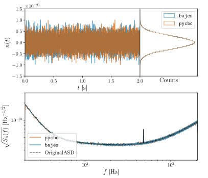
Aiming to data analysis purposes, bajes implements a Noise object. This component is capable to estimate the PSD of a given noise time-domain series using the Welch's method, generate an artificial segments of stationary and Gaussian noise from a given PSD, and it disposes of methods for PSD interpolation. Figure 3 shows a comparison of artificial noise segments generated with bajes and with the pycbc routines Usman et al. (2016); Biwer et al. (2019); Nitz et al. (2018, 2021), where the total length of the artificial segment is 1024 s. The histograms and the PSDs show that the generated noise fluctuations respect the conditions of Gaussianity and stationarity with a frequency spectrum described by the requested PSD.

Figure 3: Top left panel: Comparison of artificial noise segment produced using bajes (blue) and pycbc (orange). The segments are computed using LIGO design sensitivity P1200087 Abbott et al. (2018b) with a lower cutoff-frequency at 20 Hz and a sampling rate of 4096 Hz. The panel shows a 2 s segment extracted from a segment with total duration of $T=1024~{}{\rm s}$. Top right panel: Histograms of the time-domain samples computed using the whole artificial segment of length $T=1024~{}{\rm s}$. Bottom panel: ASDs reconstructed from the artificial noise segments using the Welch's method. The spectra are computed using the whole segments with a chuck length of 4 s and an overlap fraction of 99%. The black dashed line represents the original ASD.

IV.3 Ground-based interferometers

The current ground-based observatories for GW detection are L-shaped Michelson interferometers with Fabry-Perot cavities Dooley (2015); Akutsu et al. (2019). Each arm has a length of $L\approx 3{-}4~{}{\rm km}$, depending on the actual detector Aasi et al. (2015); Acernese et al. (2015), and it is constituted of two mirrors acting like test-masses. The detector performs measurements of the gravitational strain as a difference in length of the orthogonal arms,

$$d(t)=\frac{\Delta L(t)}{L}\,,$$ (15)

where $\Delta L=\Delta L_{x}-\Delta L_{y}$ is the difference between the displacements along the two orthogonal arms. The projection of the signal on the detector can be computed from the GW polarization components $h_{+,\times}$ as

$$h(t)=D_{ij}h_{ij}(t)=F_{+}h_{+}(t)+F_{\times}h_{\times}(t)\,,$$ (16)

where $D_{ij}$ is labeled as detector tensor and it depends on the geometry of the interferometer, while $F_{+,\times}$ are the antenna pattern functions for each polarization. The antenna patterns $F_{+,\times}$ characterize the detector sensitivity in the different regions of the sky for every given time Raymond and Farr (2014).

Generally, in standard observing conditions, the observations of GW transients are performed simultaneously by a worldwide network of ground-based interferometers. Thanks to this, it is possible to correlate strains observed independently in different locations, improving the estimation of the the astrophysical origin of the transients Nitz et al. (2019); Pankow et al. (2018).

The necessity to localize a GW observatory in a fixed frame arises, in order to project the expected signal on the detector and to estimate the light travel time from each detector in the network. For these tasks, bajes disposes of a Detector class able to characterize a ground-based interferometer. This object is identified with the coordinates of the site of the interferometer (latitude, longitude and altitude) and the angles of the two arms (azimuth and tilt). It is also possible to initialize the Detector object to precomputed detector configurations using the two-digits string identifying a ground-based interferometer, e.g. H1 for LIGO-Hanford Aasi et al. (2015), L1 for LIGO-Livingston Aasi et al. (2015), V1 for Virgo Acernese et al. (2015), G1 for GEO600 Luck et al. (2010); Dooley (2015), K1 for KAGRA Aso et al. (2013); Akutsu et al. (2020) and ET for Einstein Telescope (configuration D) Punturo et al. (2010); Hild et al. (2011).

IV.4 Waveform templates

The last ingredient necessary to complete the framework is a waveform template, i.e. a model able to compute the expected representation of the signal $h(t,\bm{\theta})$ (or ${h}(f,\bm{\theta})$) for every given set of parameters $\bm{\theta}$. The Waveform object is a class that access the methods disposable in the bajes.obs.gw.approx sub-module, and computes the expected GW polarization components for every given set of parameters. The frequency-domain waveform in Eq. (16) can be written in terms of the amplitude $A(f)$ and the phase $\phi(f)$,

$$h(f)=A(f)\,e^{-{\rm i}\big{[}\phi_{0}+2\pi t_{0}f+\phi(f)\big{]}}\,,$$ (17)

where $\phi_{0}$ and $t_{0}$ are respectively phase and time references.

bajes directly implements and interfaces with all the most advanced GW templates for quasi-circular compact binary mergers, and includes state-of-art templates for eccentric and hyperbolic binary black hole (BBH) mergers Chiaramello and Nagar (2020); Nagar et al. (2020a) as well as for BNS postmerger Breschi et al. (2019b). In particular:

• TaylorF2: The post-Newtonian (PN) framework  Blanchet et al. (1990); Faye et al. (2012); Levi and Steinhoff (2016a, b); Mishra et al. (2015); Levi and Steinhoff (2016c) represents a milestone for the description of the two-body problem. This approach solves the dynamical evolution of a compact binary with a perturbative method assuming low velocities and weak field approximations, which are reflected in the condition $v=(\pi\,GMf)^{1/3}\ll c$, where $v$ is the characteristic velocity in the binary, $M=m_{1}+m_{2}$ is the total mass and $f$ is the GW frequency. The exact analytic solution of the gravitational radiation emitted by a point-particle compact binary is known up to the 3.5PN order. bajes also implements a pseudo-5.5PN accurate description of the point mass baseline, as derived in Ref. Messina et al. (2019). Pure tidal corrections are implemented up to 7.5PN Vines et al. (2011); Damour et al. (2012) and include the recently computed tail terms (6.5, 7.5 PN) of Henry et al. (2020), whereas spin-quadrupole terms are included up to 3.5PN Nagar et al. (2019a).

• TEOBResumS: The effective-one-body (EOB) formalism  Buonanno and Damour (1999, 2000); Damour et al. (2000); Damour (2001); Damour et al. (2008, 2015); Bini et al. (2019, 2020a, 2020b) is an Hamiltonian approach that reduces the two-body problem to a single orbiting object in an effective potential. TEOBResumS Nagar et al. (2018) is an EOB approximant for spinning coalescing compact binaries Damour and Nagar (2014); Nagar et al. (2017) (black holes or neutron stars) inspiralling along generic orbits. It includes tidal effects Bini and Damour (2014); Bernuzzi et al. (2015a); Akcay et al. (2019) and subdominant modes Nagar et al. (2019b, 2020b) up to $\ell=5$, as well as a description of precession-induced modulations up to merger Akcay et al. (2020). When considering systems evolving along quasi-circular orbits, the computational performance of the model is enhanced by means of a post-adiabatic description of the early inspiral Nagar and Rettegno (2019). Moreover, the model includes the implementations of hyperbolic encounters Nagar et al. (2020a), eccentric mergers Chiaramello and Nagar (2020) and a frequency domain approximation valid for quasi-circular BNS coalescences, labeled as TEOBResumSPA Gamba et al. (2020a). The model is publicly available at teo and used in bajes from the provided Python interface.

• NRPM: BNS merger remnants are expected to be loud sources of GWs Takami et al. (2015); Clark et al. (2016); Radice et al. (2018a), that convey unique information on the equation of state of hot matter at extreme densities Radice et al. (2017, 2018b); Abbott et al. (2018a). NRPM Breschi et al. (2019b) is a analytical model based on numerical relativity BNS simulations. The model is tuned on a set of simulations covering the range $q\leq 1.5$ and $\Lambda_{1,2}\gtrsim 400$. For smaller values of the tidal parameters, the model is identically zero since it is not expected to have a post-merger signal in these cases, due to prompt black-hole formation Zappa et al. (2018); Agathos et al. (2020); Bernuzzi et al. (2020). NRPM is directly implemented in bajes and it can be attached to the TEOBResumS pre-merger template, obtaining a complete model for the gravitational radiation expected from BNS coalescences.

• MLGW: Machine learning tools can be employed to construct accurate representations of GW signals. The mlgw package Stefano Schmidt and Walter Del Pozzo (2020); Schmidt et al. (2020) takes advantage of these methods to generate fast and reliable GW templates for BBH coalescences. The model is composed by contributions extracted with principal component analysis and a linear combination of regression models, which maps the orbital parameters of the black holes to the reduced representation of the wave. A complete model includes two principal component models, for both phase and amplitude of the wave, and a mixture of regression models for each of the principal components considered. The algorithm is trained on time-domain models and tested only for aligned spin BBHs. Currently, the released software provides the representations of EOB templates, TEOBResumS Nagar et al. (2018) and SEOBNRv4 Bohé et al. (2017).

• GWSurrogate: The templates provided by the gwsurrogate package Blackman et al. implements fast waveforms based on reduced-order models Field et al. (2014) trained on numerical relativity simulations. The NRSur7dq4 model Varma et al. (2019a) is a precessing extension of the model presented in Ref. Blackman et al. (2017) trained on a set of simulations with $q\leq 4$ and $\chi_{1},\chi_{2}\leq 0.8$ that contains all higher-order modes with $\ell\leq 4$. On the other hand, NRHybSur3dq8 Varma et al. (2019b) and its tidal version Barkett et al. (2020) are calibrated using hybridized waveforms in order to increase the number of orbits of the training templates, improving the quality of the approximation. This model is tuned in a wider range in the mass ratio, $q\leq 8$, but it does not include precession contributions.

• LALSimulation: The LIGO Algorithm Library LALSuite LIGO Scientific Collaboration (2018a) is the official LIGO-Virgo Collaboration software and it provides the largest variety of waveform template models. bajes implements the waveform generator of LALSimulation, a module of LALSuite. For the results of this paper, we make use of this implementation in order to employ IMRPhenomPv2 approximant Husa et al. (2016); Khan et al. (2016) and its tidal extension, IMRPhenomPv2_NRTidal Dietrich et al. (2017). A list of all the approximants available through LALSimulation can be found at LIGO Scientific Collaboration (2018b)

V Pipeline

bajes provides a customized and automatized pipeline for the analysis of GW transients and EM counterparts. In this section, we discuss the model implemented to perform PE analysis on GW transients with bajes.

In the context of GW data analysis, we introduce the working hypotheses that are going to define the employed Bayesian model. We call the assumption that the data contains a non-vanishing GW transient signal hypothesis $H_{\rm S}$ i.e. $d(t)=n(t)+s(t)$ with $s(t)\neq 0$. On the other hand, the noise hypothesis $H_{\rm N}$ is the condition for which the recorded data corresponds only to pure noise realization, i.e. $d(t)=n(t)$. Then, in the signal hypothesis condition, a GW signal emitted by a quasi-circular compact binary coalescence (CBC) can be fully characterized with a set of 17 parameters according to General Relativity. Precisely,

$$\bm{\theta}_{\rm cbc}=\{m_{1},m_{2},\bm{\chi}_{1},\bm{\chi}_{2},\Lambda_{1},\Lambda_{2},D_{L},\iota,\alpha,\delta,\psi,t_{0},\phi_{0}\}$$ (18)

where:

• $m_{1,2}$ refer to the detector-frame masses of the two objects, taken with the convention $m_{1}{\geq}\,m_{2}$;

• $\bm{\chi}_{1,2}$ are the dimensionless spin vectors,

  $$\bm{\chi}_{i}=\frac{c\,\textbf{S}_{i}}{Gm_{i}^{2}}\,,\quad\,i=1,2\,,$$ (19)

  where $\textbf{S}_{1,2}$ are the spins of the two objects, $c$ is the speed of light and $G$ is the gravitational constant.

• $\Lambda_{1,2}$ are the dimensionless tidal polarizability parameters that encode the quadrupolar deformability of the $i$-th object under the effect of an external force,

  $$\Lambda_{i}=\frac{2}{3}\,k_{2,i}\,\left(\frac{c^{2}\,R_{i}}{Gm_{i}}\right)^{5}\,,\quad\,i=1,2\,,$$ (20)

  where $k_{2,i}$ and $R_{i}$ are respectively the second Love number and the radius of the $i$-th object ($k_{2}$ is identically zero for black holes).

• $D_{L}$ is the luminosity distance of the source from the observer;

• $\iota$ is the angle between the line of sight and the total angular momentum of the system and it takes value in the range $[0,\pi]$,

• $\{\alpha,\delta\}$ are respectively right ascension and declination angles that identify the sky position of the source;

• $\psi$ is the polarisation angle and it takes value in the range $[0,\pi]$;

• $\{t_{0},\phi_{0}\}$ are respectively reference time and reference phase.

The sampling is performed promoting the chirp mass $\mathcal{M}$ and the mass ratio $q$,

$$\mathcal{M}=\frac{(m_{1}m_{2})^{3/5}}{(m_{1}+m_{2})^{1/5}}\,,\quad q=\frac{m_{1}}{m_{2}}\geq 1\,,$$ (21)

over the single mass components, since they appear to be less correlated for this type of signals Veitch and Vecchio (2010); Veitch et al. (2015). For spinning binary mergers, we define the effective spin parameter $\chi_{\rm eff}$ as

$$\chi_{\rm eff}=\frac{m_{1}\chi_{1,z}+m_{2}\chi_{2,z}}{m_{1}+m_{2}}\,,$$ (22)

that encodes the aligned-spin contribution and it can lead to narrower uncertainties than the single spin components Ng et al. (2018). Furthermore, in the context of BNS mergers, it is useful to introduce the reduced tidal parameter $\tilde{\Lambda}$,

$$\tilde{\Lambda}=\frac{16}{13}\left[\frac{(m_{1}+12m_{2})m_{1}^{4}\Lambda_{1}}{M^{5}}+(1\leftrightarrow 2)\right]\,$$ (23)

and the asymmetric tidal parameter ${\delta\tilde{\Lambda}}$,

$${\delta\tilde{\Lambda}}=\left[1-\frac{7996}{1319}\frac{m_{2}}{m_{1}}-\frac{11005}{1319}\left(\frac{m_{2}}{m_{1}}\right)^{2}\right]\frac{m_{1}^{6}\Lambda_{1}}{M^{6}}-(1\leftrightarrow 2)\,,$$ (24)

where $M=m_{1}+m_{2}$. The tidal parameters ${\tilde{\Lambda}}$ and ${\delta\tilde{\Lambda}}$ are respectively proportional to the leading order and the next-to-leading order tidal contributions according with PN expansion.

Generally, concerning GW analysis, it is common to label $\bm{\theta}_{\rm int}=\{m_{1},m_{2},\bm{\chi}_{1},\bm{\chi}_{2},\Lambda_{1},\Lambda_{2}\}$ as intrinsic parameters, since they affect the physical dynamics of the system; while, the extrinsic parameters $\bm{\theta}_{\rm ext}=\{D_{L},\iota,\alpha,\delta,\psi,t_{0},\phi_{0}\}$ are related with the observed signal by trivial geometrical argumentation. Moreover, it is possible to include in the pipeline further parameters in order to take into account the calibration of the input quantities, such as calibration envelopes and PSD uncertainties. For a detailed discussion about these topics, see Sec. V.4.

In the following sections, we present the implementations available in the bajes GW pipeline.

V.1 Data segments

The default GW routine implemented in bajes is designed for binary mergers analyses. In general, the pipeline is able to access to the open-source database of GWOSC Abbott et al. (2019d); Trovato (2020); LIGO Scientific and Virgo Collaboration (a), to all the data released with GWTC-1 Abbott et al. (2019a) and to the expected PSD curves for current and next-generation detectors Punturo et al. (2010); Hild et al. (2011).

The input data to be analyzed by the pipeline can be gathered in different ways. The GW pipeline provides a customized injection generator capable to produce artificial data given a prescribed set of parameters and the detector sensitivity curves. Moreover, the bajes pipeline allows to access the observational data recorded by the LIGO-Virgo interferometers Abbott et al. (2018b); Aasi et al. (2015); Acernese et al. (2015) from the GWOSC, specifying the central value of the GPS time and the duration of the segment.

When the data information is gathered, the pipeline initializes the Likelihood function and the Prior with the requested parameters belonging to the set $\bm{\theta}_{\rm cbc}$, and it passes these arguments to the requested sampler which performs the Bayesian inference.

V.2 Prior distributions

The prior distribution for the masses is chosen flat in the components $\{m_{1},m_{2}\}$, that can be written in terms of $\{\mathcal{M},q\}$ as

$$p(\mathcal{M},q|H_{\rm S})=\frac{\mathcal{M}}{\Pi_{\mathcal{M}}\Pi_{q}}\,\left(\frac{1+q}{q^{3}}\right)^{2/5}\,,$$ (25)

where $\Pi_{\mathcal{M}}$ and $\Pi_{q}$ are the prior volumes limited by the bounds $[\mathcal{M}_{\rm min},\mathcal{M}_{\rm max}]$ in chirp mass and $[1,q_{\rm max}]$ in mass ratio,

$$\begin{split}\Pi_{\mathcal{M}}&=\frac{1}{2}\left(\mathcal{M}^{2}_{\rm max}-\mathcal{M}_{\rm min}^{2}\right)\,,\\ \Pi_{q}&=5\left[\frac{2^{2/5}\sqrt{\pi}\,\Gamma\left(\frac{4}{5}\right)}{\Gamma\left(\frac{3}{10}\right)}-\frac{{}_{2}F_{1}\left(-\frac{2}{5},-\frac{1}{5},\frac{4}{5},-q_{\rm max}\right)}{q_{\rm max}^{1/5}}\right]\,,\\ \end{split}$$ (26)

where ${}_{2}F_{1}(a,b,c;z)$ is the hypergeometric function and $\Gamma(x)$ is the Euler function.

The spin vectors can be written in the polar frame of the binary as $\bm{\chi}_{i}=\{\chi_{i},\vartheta_{i},\varphi_{i}\}$, where $\chi_{i}$ is the spin magnitude, $\vartheta_{i}$ is the tilt angle and $\varphi_{i}$ is the complimentary azimuthal angle between $\bm{\chi}_{i}$ and the orbital angular momentum L of the binary. The prior distribution for these quantities is specified by the maximum value of spin magnitude $\chi_{\rm max}\geq 0$ and it can be chosen between the following:

• Isotropic prior with precessing spins: the prior on the angular components $\{\vartheta_{i},\varphi_{i}\}$ is isotropic over the solid angle, while the spin magnitude is uniformly distributed in the range $[0,\chi_{\rm max}]$,

  $$p(\chi_{i},\vartheta_{i},\varphi_{i}|H_{\rm S})=\frac{\sin\vartheta_{i}}{4\pi\chi_{\rm max}}\,.$$ (27)

• Isotropic prior with aligned spins: this case is identical to the isotropic one except for the assumption of aligned spins, $\vartheta_{i}=0,\pi$. The $xy$ components of the spin vectors are marginalized, obtaining the form Lange et al. (2018)

  $$p(\chi_{i,z}|H_{\rm S})=\frac{1}{2\chi_{\rm max}}\log\left|\frac{\chi_{\rm max}}{\chi_{i,z}}\right|\,.$$ (28)

• Volumetric prior with precessing spins: the distribution is taken uniform in all Cartesian components, i.e. flat over the sphere with radius $\chi_{\rm max}$. This prior can be written as

  $$p(\chi_{i},\vartheta_{i},\varphi_{i}|H_{\rm S})=\frac{3}{4\pi}\,\frac{\chi_{i}^{2}\sin\vartheta_{i}}{\chi^{3}_{\rm max}}\,.$$ (29)

• Volumetric prior with aligned spins: the same of volumetric case with aligned components; the marginalization over the $xy$ components leads to the form

  $$p(\chi_{i,z}|H_{\rm S})=\frac{9}{16\pi}\frac{\chi^{2}_{\rm max}-\chi_{i,z}^{2}}{\chi^{3}_{\rm max}}\,.$$ (30)

The prior distribution for the sky position parameters $\{\alpha,\delta\}$ is taken isotropic over the entire solid angle, such that $\alpha\in[0,2\pi]$ and $\delta\in[-\pi/2,+\pi/2]$,

$$p(\alpha,\delta|H_{\rm S})=\frac{\cos\delta}{4\pi}\,,$$ (31)

and analogously for the inclination $\iota$ in the range $[0,\pi]$,

$$p(\iota|H_{\rm S})=\frac{\sin\iota}{2}\,.$$ (32)

Regarding the luminosity distance the bounds are specified by the lower and the upper bounds $[D_{\rm min},D_{\rm max}]$, and the analytic form of the prior can be chosen between the followings:

• Volumetric prior: general analysis assumes that the source is uniformly distributed over the sphere centred around the detectors, then

  $$p(D_{L}|H_{\rm S})=\frac{3D_{L}^{2}}{D_{\rm max}^{3}-D_{\rm min}^{3}}\,.$$ (33)

• Comoving-volumetric prior: in order to take into account the cosmological expansion of the Universe, a prior uniformly distributed over the comoving volume $V_{C}$ is a more suitable physically-motivated choice. Within this assumption, the prior on the luminosity distance can be written as

  $$p(D_{L}|H_{\rm S})\propto\frac{\text{d}V_{C}}{\text{d}D_{L}}\,.$$ (34)

  The luminosity distance $D_{L}$ and the comoving volume $V_{C}$ are related through the redshift $z$ for a fixed cosmological model; by default, bajes acquires the values of the cosmological constants from Ref. Aghanim et al. (2020).

• Source-frame prior: as shown in Ref. Abbott et al. (2019c, 2020a), Eq. (34) does not take into account contributions due to time dilatation. Then, we can introduce a prior distribution uniformly distributed in the source-frame volume as

  $$p(D_{L}|H_{\rm S})\propto\frac{1}{1+z}\cdot\frac{\text{d}V_{C}}{\text{d}D_{L}}\,,$$ (35)

  where the factor $(1+z)^{-1}$ converts the merger rate from the source frame to the detector frame.

• Log-uniform prior: it could be useful to introduce a uniform prior in $\log D_{L}$, then

  $$p(D_{L}|H_{\rm S})=\frac{D_{L}^{-1}}{\log\left(D_{\rm max}/D_{\rm min}\right)}\,.$$ (36)

For the remaining parameters, i.e. $\{\psi,t_{0},\phi_{0}\}$ and $\{\Lambda_{1},\Lambda_{2}\}$ (if required), their prior distributions are taken uniform within the provided bounds. Then, the overall prior is the product of the priors of the single parameters.

V.3 Likelihood function

The key ingredient of the inference is the likelihood function, that encodes the capability of a given model $h(t,\bm{\theta}_{\rm cbc})$ to match the observed data $d(t)$. For Gaussian and stationary noise $n(t)$, we expect the mean of the noise fluctuations to be centered around zero with a variance described by the PSD in the frequency-domain, i.e.

$$p(n|H_{\rm N})\propto e^{-\frac{1}{2}(n|n)}\,.$$ (37)

It follows that, within the signal hypothesis $H_{\rm S}$ and supposing that we dispose of a template $h(t,\bm{\theta}_{\rm cbc})$ capable to reproduce the real signal $s(t)$ for a given set of $\bm{\theta}_{\rm cbc}$, the log-likelihood function can be written as the frequency-domain residuals between the recorded data and the template with the product defined in Eq. (10),

$$p(d|\bm{\theta}_{\rm cbc},H_{\rm S})=\frac{1}{\mathcal{N}}\,e^{-\frac{1}{2}(d-h|d-h)}\,.$$ (38)

where $\mathcal{N}$ is the normalisation constant, that can be expressed in terms of the PSD using the numerical approximation Eq. (12),

$$\mathcal{N}\approx\prod_{i}\sqrt{\frac{\pi\,T\,S_{n}(f_{i})}{2}}\,.$$ (39)

Then, the Bayes's factor of the signal hypothesis against the noise assumption can be computed as

$$\mathcal{B}^{\rm S}_{\rm N}=\frac{p(d|H_{\rm S})}{p(d|H_{\rm N})}=\int_{\bm{\Theta}}\exp\left[\big{(}d\big{|}h(\bm{\theta}_{\rm cbc})\big{)}-\frac{1}{2}\big{(}h(\bm{\theta}_{\rm cbc})\big{|}h(\bm{\theta}_{\rm cbc})\big{)}\right]\,p(\bm{\theta}_{\rm cbc}|H_{\rm S})\,\text{d}\bm{\theta}_{\rm cbc}\,.$$ (40)

Combining Eq. (38) with Eq. (17), it is possible to write the explicit dependency of the likelihood with respect to the reference parameters $\{\phi_{0},t_{0}\}$, since these values have no physical relevance, we marginalize the posterior distribution with respect to $\{\phi_{0},t_{0}\}$ in order to increase the efficiency of the sampling. The marginalization over $\phi_{0}$ can be computed analytically and the solution can be written in terms of the modified Bessel function of the first kind Veitch and Del Pozzo . For the time-shift $t_{0}$, the computation is semi-analytical since the values of the likelihood are evaluated on a equally-spaced grid resorting on the FFT computation Farr .

V.4 Additional implementations

In order to perform accurate and reliable inferences of GW transients, the pipeline requires refinements and auxiliary control systems. In this section we discuss some of the additional tools implemented in the GW pipeline supplied with bajes.

V.4.1 Calibration envelopes

The necessity of calibration envelopes Vitale et al. (2012) arises due to imperfect knowledge of the interferometer response to differential arm length changes Abbott et al. (2017d); Cahillane et al. (2017); Acernese et al. (2018), which affects the transfer functions of the detector components introducing systematic errors that propagate to the recorded data. These uncertainties are estimated by inspecting the detector control systems and propagating the measurements into a frequency-dependent probability distribution. Subsequently, the information on calibration errors must be taken into account when inferring the astrophysical parameters of GW signals. In order to achieve this task, it is useful to introduce two auxiliary functions $\delta A(f)$ and $\delta\phi(f)$ that characterise respectively the amplitude and the phase uncertainties of the measured data segments. Then, the calibration envelopes $\{\delta A(f),\delta\phi(f)\}$ can be taken into account in the Bayesian model as

$$h(f)\to\big{[}1+\delta A(f)\big{]}\,e^{{\rm i}\delta\phi(f)}\,h(f)\,.$$ (41)

This procedure is accomplished specifying the values of the calibration envelopes at predefined logarithmic-spaced frequency nodes $f_{j}$ and linearly interpolated over the interested frequency axis. The calibration parameters $\{\delta A(f_{j}),\delta\phi(f_{j})\}$ are introduced in the sampling and estimated along with the signal parameters. The prior for calibration envelopes $\{\delta A(f_{j}),\delta\phi(f_{j})\}$ is a multivariate normal distribution with variance specified by the measured calibration errors.

V.4.2 PSD uncertainties

The usage of a fixed estimated PSD might generate biases due to non-stationary effects and unaccounted slow variations in the noise spectrum. Then, it arises the necessity to take into account the uncertainty of the PSD estimate during the inference of the properties of a GW signal. For this reason, the pipeline allows the possibility to include PSD uncertainty weights $\eta_{j}$ Veitch et al. (2015): the Fourier domain is dived in predefined logarithmic-spaced bins $[f_{j},f_{j+1}]$ and the weights are included such that

$$S_{n}(f)\to\eta_{j}\,S_{n}(f)\,,\quad{\rm for}\,f_{j}\leq f<f_{j+1}\,,$$ (42)

where $\eta_{j}$ is taken constant in respective frequency bin. The full set of $\{\eta_{j}\}$ parameters, one for every frequency bin, is introduced in the sampling and they are estimated during the exploration with the signal parameters. The prior distribution for the PSD uncertainty $\eta_{j}$ is take normal with mean zero and variance $1/N_{j}$, where $N_{j}$ is the number of data sample enclosed in the bin $[f_{j},f_{j+1}]$. This scheme has shown to improve the robustness of the GW inference Littenberg et al. (2013) and it offers a flexible model capable to quantify the differences between the estimated PSD and the spectrum of the analyzed data.

VI Injection studies

In this section, we show the results coming from a set of injection studies performed with the bajes pipeline, in order to test the sampling routines with the GW infrastructure. An injection is a simulated GW signal that has been added into a time-domain segment. For our studies, we generate artificial noise segments according with a prescribed PSD assuming Gaussian and stationary fluctuations, as discussed in Sec. IV.2. Subsequently, the artificial signal $h(t)$ is simulated according with the input parameters $\bm{\theta}_{\rm cbc}$, projected on the requested detectors and included in the data segment. Finally, the data are analyzed by the bajes pipeline resorting to the framework described above. The sensitivity curves employed for these studies correspond to the noise spectra expected at design sensitivity for current ground-based detector Aasi et al. (2015); Abbott et al. (2018b); Harry (2010); Acernese et al. (2015); Aso et al. (2013); Akutsu et al. (2019) and for next-generation interferometers Punturo et al. (2010); Hild et al. (2011). The properties of the injected signals are described in the following paragraphs depending on the particular kind of source.

Table 1: Recovered parameters during the BBH injections studies. The signal has been injected in H1+L1 using design sensitivity curves, with an overall network SNR of 14. The data has been analyzed with the bajes PTMCMC sampling. The reported values correspond to the medians with the 90% credible regions. The last column reports the estimated logarithmic Bayes' factor and the associated standard deviation.

Approximant	$\mathcal{M}$	$q$	$\chi_{1,z}$	$\chi_{2,z}$	$\chi_{\rm eff}$	$D_{L}$	$\iota$	$\alpha$	$\delta$	$\log\mathcal{B}^{\rm S}_{\rm N}$
	$[{\rm M_{\odot}}]$					$[{\rm Gpc}]$	$[{\rm rad}]$	$[{\rm rad}]$	$[{\rm rad}]$
Injected	30.0	2.0	0.3	0.0	0.2	3.0	0.0	0.372	0.811	–
TEOBResumS	${30.63}^{+1.84}_{-1.64}$	${1.56}^{+0.78}_{-0.49}$	${0.24}^{+0.36}_{-0.41}$	${0.17}^{+0.59}_{-0.63}$	${0.23}^{+0.14}_{-0.15}$	${2.49}^{+1.29}_{-1.17}$	${0.82}^{+2.05}_{-0.63}$	${2.17}^{+4.05}_{-2.13}$	${0.21}^{+1.10}_{-1.09}$	${73.29}^{+2.64}_{-2.64}$
IMRPhenomPv2	${30.34}^{+1.77}_{-1.69}$	${1.50}^{+0.83}_{-0.46}$	${0.17}^{+0.43}_{-0.43}$	${0.17}^{+0.57}_{-0.60}$	${0.19}^{+0.14}_{-0.16}$	${2.47}^{+1.30}_{-1.22}$	${0.80}^{+2.06}_{-0.62}$	${2.34}^{+3.88}_{-2.31}$	${0.17}^{+1.13}_{-1.05}$	${73.16}^{+2.66}_{-2.66}$
NRSur7dq4	${30.35}^{+1.75}_{-1.60}$	${1.56}^{+0.82}_{-0.53}$	${0.18}^{+0.37}_{-0.39}$	${0.17}^{+0.59}_{-0.63}$	${0.19}^{+0.56}_{-0.63}$	${2.49}^{+1.25}_{-1.23}$	${0.84}^{+2.02}_{-0.64}$	${2.11}^{+4.12}_{-2.07}$	${0.21}^{+1.10}_{-1.09}$	${73.11}^{+2.72}_{-2.72}$

VI.0.1 Binary black holes

The first example corresponds to an aligned-spinning BBH coalescence with intrinsic parameters {$\mathcal{M}=30~{}{\rm M_{\odot}}$, $q=2$, $\chi_{1,z}=0.3$, $\chi_{2,z}=0.$} located at a luminosity distance $D_{L}=3~{}{\rm Gpc}$ with inclination angle $\iota=0$. The signal is injected such that the merger occurs at GPS time 1126259462.0 with a sampling rate of 4096 Hz and a signal length of $16~{}{\rm s}$. The data are analyzed using two detectors, H1 and L1, with LIGO design sensitivity P1200087 Aasi et al. (2015); Abbott et al. (2018b); Harry (2010). The sky location of the source corresponds to the position of maximum sensitivity for the detector H1, $\{\alpha=0.372,\delta=0.811\}$. The injected signal is generated with TEOBResumS waveform model (employing only the dominant mode) with a network SNR of 14, corresponding to 11 in H1 and 9 in L1.

The recovery of the posterior distribution is performed with PTMCMC sampling with 8 tempered ensembles and 128 chains per ensemble. Moreover, we requested $8{\times}10^{3}$ burn-in iterations. The injected strain is analyzed in the frequency domain from 20 Hz to 1 kHz employing three different templates: TEOBResumS, IMRPhenomPv2 and NRSur7dq4. The likelihood is marginalized over reference time and phase. We set the chirp mass prior in $[23,37]\,{\rm M_{\odot}}$ and the mass ratio in $[1,8]$. The spins are kept aligned with an isotropic prior in the range $[-0.9,+0.9]$ for every component. We employ volumetric prior for the luminosity distance in the support $[100~{}{\rm Mpc},5~{}{\rm Gpc}]$ and the prior distributions for the remaining parameters are chosen according with Sec. V.2.

Figure 4: Sampler acceptances during the BBH injection study performed with TEOBResumS described in Sec. VI.0.1. The blue line is the proposal acceptance of the untempered ensemble averaged over the chains, the yellow and the green lines are respectively the proposal and the swapping acceptances of whole sampler averaged over all the tempered ensembles. The solid lines represent the median values and the shadowed areas are the 90% credible regions. The vertical black line is the requested last burn-in iteration.

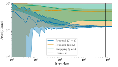
Figure 4 shows the acceptance fractions for the analysis performed with TEOBResumS waveform model. The inferences performed with other approximants shown similar behaviours. The untempered ensemble required less then $10^{4}$ iterations to converged to the maximum-posterior value. After the requested burn-in, the untempered ensemble shown an average acceptance of $15\%$ and, averaging over all the tempered ensembles, the sampler advanced with a global proposal acceptance of ${\sim}45\%$ and with a global swapping acceptance of ${\sim}50\%$. The final autocorrelation length (ACL) of the untempered ensemble corresponds to a lag of 70 iterations and the sampler collected a final amount of $1.5{\times}10^{4}$ independent posterior samples.

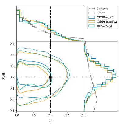
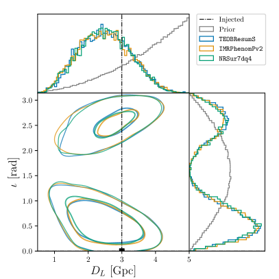
Table 1 shows the recovered mean values and Figure 5 shows the recovered marginalized posterior distribution for some exemplary parameters. The marginalized posterior distributions enclose the injected values within 90% credible intervals for all the waveform approximants. The estimated evidences slightly prefer TEOBResumS waveform, accordingly with the injected template. However, these values lie in the same range for all the analyses, leading to a not fully resolved model selection. This is due to the large uncertainties associated to the evidence estimation of the PTMCMC and with the relatively low SNR of the injected signal. For the latter reason, it is also not possible to reveal systematic differences between the different approximants Abbott et al. (2017e), and the results of the employed templates are largely consistent between each other.

Figure 5: Posterior distributions for $\{q,\chi_{\rm eff}\}$ and $\{D_{L},\iota\}$ recovered from the injection studies performed on a BBH signal with two inteferometers (H1+L1) at design sensitivities with network SNR of 14. The artificial signal has been generated with TEOBResumS model and the injected parameters are marked with black lines and squares. The contours represent the 50% (thick) and the 90% (thin) credible regions. The recovery has been performed with four different approximants analysing the frequency range from 20 Hz to 1 kHz. The estimation of the luminosity distance is affected by the degeneracy with the inclination angle Abbott et al. (2016b), due to the correlations in the strain amplitude for aligned-spin sources.

VI.0.2 Binary neutron stars inspiral

Table 2: Recovered parameters during the inpiralling BNS injections studies. The signal has been injected in H1+L1 using design sensitivity curves, with an overall network SNR of 20. The data has been analyzed with the nested sampling provided by dynesty. The reported values correspond to the medians with the 90% credible regions. The last column reports the estimated logarithmic Bayes' factor and the associated standard deviation.

Approximant	$\mathcal{M}$	$q$	$\chi_{\rm eff}$	${\tilde{\Lambda}}$	$D_{L}$	$\iota$	$\alpha$	$\delta$	$\log\mathcal{B}^{\rm S}_{\rm N}$
	$[{\rm M_{\odot}}]$				$[{\rm Mpc}]$	$[{\rm rad}]$	$[{\rm rad}]$	$[{\rm rad}]$
Injected	1.188	1.00	0.00	600	120	0.00	0.372	0.811	–
TEOBResumSPA	${1.1880}^{+0.0002}_{-0.0002}$	${1.20}^{+0.42}_{-0.17}$	${0.01}^{+0.05}_{-0.01}$	${435}^{+305}_{-248}$	${113}^{+19}_{-38}$	${0.60}^{+1.98}_{-0.42}$	${0.48}^{+0.26}_{-0.12}$	${0.86}^{+0.20}_{-0.21}$	${564.6}^{+0.3}_{-0.3}$
TaylorF2	${1.1880}^{+0.0005}_{-0.0001}$	${1.28}^{+1.16}_{-0.25}$	${0.01}^{+0.10}_{-0.01}$	${392}^{+415}_{-260}$	${106}^{+26}_{-38}$	${0.82}^{+1.91}_{-0.56}$	${0.75}^{+3.51}_{-0.33}$	${0.81}^{+0.28}_{-1.56}$	${564.3}^{+0.3}_{-0.3}$
IMRPhenomPv2NRT	${1.1880}^{+0.0002}_{-0.0001}$	${1.25}^{+0.36}_{-0.21}$	${0.01}^{+0.02}_{-0.01}$	${316}^{+304}_{-215}$	${111}^{+20}_{-50}$	${0.76}^{+1.98}_{-0.55}$	${0.63}^{+3.54}_{-0.21}$	${0.79}^{+0.24}_{-1.49}$	${563.9}^{+0.3}_{-0.3}$

In this section we analyse an inspiralling nonspinning BNS merger with intrinsic parameters are {$\mathcal{M}=1.188~{}{\rm M_{\odot}}$, $q=1$, $\Lambda_{1}=\Lambda_{2}=600$}. The source is located at a luminosity distance $D_{L}=120~{}{\rm Mpc}$ with inclination angle $\iota=0$. The signal is injected such that the merger occurs at GPS time 1126259462.0 with a sampling rate of 4096 Hz and a signal length of 128 s. The data are analyzed using two detectors, H1 and L1, with LIGO design sensitivity P1200087 Aasi et al. (2015); Abbott et al. (2018b); Harry (2010). The sky location of the source corresponds to the position of maximum sensitivity for the detector H1, $\{\alpha=0.372,\delta=0.811\}$. The injected signal is generated with TEOBResumS waveform model with a network SNR of 20, corresponding to 15 in H1 and 13 in L1.

The recovery of the posterior distribution is performed employing nested sampling algorithm with 1024 live point and tolerance equal to $0.1$. Furthermore, we set respectively the minimum and the maximum number of iterations for every MCMC sub-chain to 32 and $4{\times}10^{3}$. The injected strain is analyzed in the frequency domain from 20 Hz to 1 kHz employing three different templates: TEOBResumSPA, IMRPhenomPv2_NRTidal and TaylorF2 including 5.5PN point-mass corrections and 6PN tidal contributions. We set the chirp mass prior in $[0.8,2]\,{\rm M_{\odot}}$ and the mass ratio in $[1,4]$. The spins are kept aligned with an isotropic prior in the range $[-0.9,+0.9]$ for every component. The tidal parameters are extracted in the range $[0,5000]$. We employ volumetric prior for the luminosity distance in the support $[10,400]\,{\rm Mpc}$ and the prior distributions for the remaining parameters are chosen according with Sec. V.2.

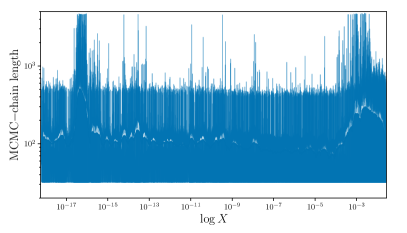
Figure 6 shows the number of iterations of the MCMC sub-chains employed to propose a new point as a function of the prior mass $X$ (see App. B for the definition). The actual values extracted from the sampler have been smoothed with a Savitzky-Golay filter for visualisation purposes. The shadowed region shows the difference between the actual MCMC-chain lengths and the filtered estimation. Large values of MCMC-chain length (say $\gtrsim 250$) characterize the more expensive steps, where the proposal method requires more iterations in order to propose a new samples and estimate the boundaries of the current contour. During the initial stages ($X{\approx}1$), the boundaries defined by the current live points were comparable with the prior and the sampler required many iterations in order to propose new samples. Subsequently, for $\log X\lesssim 10^{4}$, the sampler identified the region that encloses the majority of the posterior volume and the algorithm advanced spending ${\sim}100$ iterations to propose a new sample. The length of the MCMC-chain slightly increases again during the latest stages, since the sampler has to reach the bulk of the posterior distribution restricting the boundaries to a neighborhood of the maximum-likelihood values.

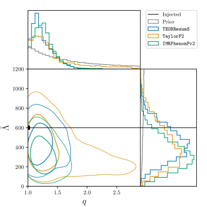
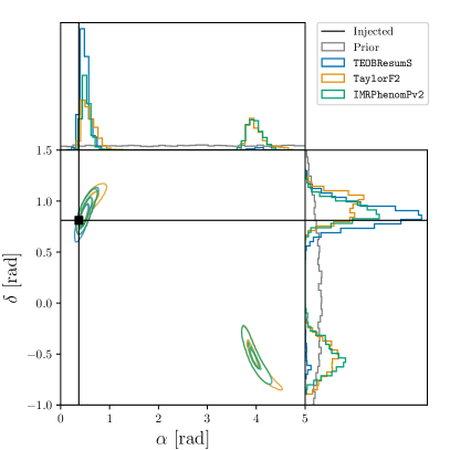
Table 2 shows the recovered median values and Figure 7 shows the marginalized posterior distribution for some exemplary parameters. The recovered values are in agreement with the properties of the injected signal: the posterior distribution encloses the injected sample for all the parameter in the 50% credible region, with a small bias in the in the maximum-posterior value for the reduced tidal parameter ${\tilde{\Lambda}}$, corresponding to roughly ${\sim}150$. However, this behavior is expected Wade et al. (2014); Abbott et al. (2019e); Dudi et al. (2018); Samajdar and Dietrich (2019); Gamba et al. (2020b) considering that we employed an upper cutoff-frequency of 1 kHz combined with the large aligned-spin prior . The estimated evidences slightly prefer TEOBResumSPA approximant, accordingly with the injected model; however, due to the low SNR, they do not show any strong preference.

Figure 6: Length of the MCMC sub-chains during the nested sampling performed with TEOBResumSPA described in Sec. VI.0.2. The actual values extracted from the sampler have been smoothed with a Savitzky-Golay filter for visualisation purposes. The shadowed region shows the difference between the actual lengths and the filtered estimation. The values are lower-bounded by the requested minimum value, set equal to 32.

Figure 7: Posterior distributions for $\{q,{\tilde{\Lambda}}\}$ and $\{\alpha,\delta\}$ recovered from the injection studies performed on an inspiralling BNS signal with two inteferometers (H1+L1) at design sensitivities with network SNR of 20. The artificial signal has been generated with TEOBResumS model and the injected parameters are marked with black lines and squares. The recovery has been performed with three different approximants analysing frequency range from 20 Hz to 1 kHz. The degeneracy in the sky location can be removed introducing a third detector Abbott et al. (2017f) and it is due to the correlations between longitudinal and latitudinal angles that concur in the estimation of times of arrival in the different interferometers.

VI.0.3 Binary neutron stars postmerger

Table 3: Recovered parameters during the BNS postmerger injection survey. The reported values correspond to the medians with the 90% credible regions.

SNR	$\mathcal{M}$	${\tilde{\Lambda}}$	$f_{2}$	$R_{\rm max}$	$\log\mathcal{B}^{\rm S}_{\rm N}$
	$[{\rm M_{\odot}}]$		$[{\rm kHz}]$	$[{\rm km}]$
Injected	1.188	600	2.94	10.8	–
8	${2.2}^{+0.8}_{-1.5}$	${2700}^{+1800}_{-1800}$	${0.8}^{+2.1}_{-0.3}$	${27}^{+10}_{-19}$	${0.2}^{+0.2}_{-0.2}$
9	${1.3}^{+1.6}_{-0.7}$	${2350}^{+1900}_{-1700}$	${1.7}^{+1.2}_{-1.1}$	${14}^{+22}_{-6}$	${2.6}^{+1.3}_{-1.3}$
10	${0.8}^{+2.2}_{-0.2}$	${2830}^{+1630}_{-1910}$	${2.7}^{+0.3}_{-2.0}$	${8.9}^{+2.8}_{-0.9}$	${11.0}^{+4.8}_{-4.8}$
12	${0.8}^{+2.1}_{-0.2}$	${1860}^{+2570}_{-1410}$	${2.9}^{+0.7}_{-2.3}$	${9.0}^{+2.7}_{-0.8}$	${13.9}^{+6.3}_{-6.3}$
16	${0.78}^{+0.43}_{-0.18}$	${1780}^{+2640}_{-1220}$	${2.93}^{+0.02}_{-0.39}$	${8.9}^{+2.0}_{-0.8}$	${45.2}^{+4.2}_{-4.2}$
32	${0.80}^{+0.45}_{-0.12}$	${1730}^{+730}_{-1220}$	${2.93}^{+0.02}_{-0.03}$	${9.0}^{+2.1}_{-0.6}$	${271}^{+29}_{-29}$

Figure 8: Marginalized posterior distributions for $\{f_{2},{\tilde{\Lambda}},R_{\rm max}\}$ recovered in the BNS postmerger injection survey using a five-detector-network H1+L1+V1+K1+ET at design sensitivities varying the luminosity distance and locating the source in the position of maximum sensitivity for ET. The injected signals have been generated with NRPM template and recovered with the same model.

Figure 9: Frequency-domain amplitude strains in the ET detector for the analysis at SNR 16 corresponding to a luminosity distance of 40 Mpc. The plotted quantities correspond to the injected signal (black), the full artificial data strain (grey) and the recovered template (blue), where the solid line is the mean value and the shadowed area is the 90% credible region.

We perform a set of BNS postmerger injections using a five-detector network which includes: H1 and L1 with LIGO design sensitivity P1200087 Aasi et al. (2015); Abbott et al. (2018b); Harry (2010), V1 with Virgo design sensitivity P1200087 Acernese et al. (2015), K1 with KAGRA design sensitivity T1600593 Aso et al. (2013); Akutsu et al. (2019) and the third-generation interferometer ET (configuration D) P1600143 Punturo et al. (2010); Hild et al. (2011). The injected signals are generated with NRPM and correspond to the postmerger radiations of non-spinning BNSs with intrinsic parameters {$\mathcal{M}=1.188~{}{\rm M_{\odot}}$, $q=1$, $\Lambda_{1}=\Lambda_{2}=600$}. The signal is injected such that the merger occurs at GPS time 1126259462.0 with a sampling rate of 8192 Hz and a signal length of 4 s. The sky location of the source corresponds to the position of maximum sensitivity for the detector ET, $\{\alpha=2.640,\delta=0.762\}$. The signals are injected at different luminosity distances in order to simulate different SNRs, spanning the range from 8 to 32, which corresponds to $D_{L}\in[20,80]~{}{\rm Mpc}$. We observe that, for these kind of signal, ET is the most relevant detector and it concurs in the determination of the SNR with a weight larger than 90% for all the analyzed cases.

For these studies, we employ the PTMCMC sampler using 8 tempered ensembles with 128 chains and $2\times 10^{4}$ burn-in iterations. The injected strain is analyzed in the frequency domain from 1 kHz to 4 kHz employing NRPM waveforms . We set the chirp mass prior in $[0.8,2]\,{\rm M_{\odot}}$ and the mass ratio in $[1,1.5]$. The spins are kept fixed to zeros for every component. The tidal parameters are extracted in the range $[0,5000]$. We employ volumetric prior for the luminosity distance in the support $[5~{}{\rm Mpc},400~{}{\rm Mpc}]$ and the prior distributions for the remaining parameters are chosen according with Sec. V.2.

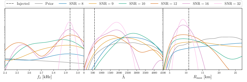
As shown in Ref. Bernuzzi et al. (2015b), the postmerger GW radiation of a long-lived BNS merger is characterized by a main frequency peak in the Fourier domain ($f_{2}$) that can be parametrized with quasiuniversal (EOS-insensitive) relations involving the tidal polarizability parameters. The NRPM model is constructed using these relations that allow one to constrain ${\tilde{\Lambda}}$ from postmerger observations and at the same time map the properties of a postmerger signal into the inspiral parameters of the binary Breschi et al. (2019b). Furthermore, numerical relativity simulations Bauswein et al. (2012); Breschi et al. (2019b) have shown that the postmerger frequency peak $f_{2}$ can be related to the radius $R_{\rm max}$ of the maximum mass configuration of a non-rotating neutron star. For the injected sources, we get $f_{2}=2.94~{}{\rm kHz}$ and $R_{\rm max}=10.8~{}{\rm km}$.

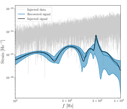
Tab 3 shows the recovered mean values and Figure 8 shows the marginalized posterior distributions for $f_{2}$ and for ${\tilde{\Lambda}}$ recovered during the survey described above and Figure 9 presents the recovered postmerger signal recovered in the ET detector for the case with SNR 16. The Bayes factors shows evidence of signal from SNR 9; however, in order to estimate $f_{2}$ with an accuracy of $O(0.1~{}{\rm kHz})$, the method requires an SNR ${\gtrsim}12$. The mean values estimated from the marginalized posteriors agree with the injected properties of the signal within the 90% credible intervals; however, it is interesting to observe that, due to the correlations induced by the EOS-insensitive relations, the sampler explores non-trivial degeneracy between the intrinsic parameters. The same behavior has been shown in Ref. Breschi et al. (2019b). These correlations strongly affect the estimation of ${\tilde{\Lambda}}$ and PE of a postmerger signal is only capable of imposing an upper bound for this parameter. For example, with SNR 32 it would be possible to constrain the value of ${\tilde{\Lambda}}$ with an uncertainty of ${\sim}10^{4}$, that is a much larger value compared with the uncertainties coming from the analysis of the inspiral data (see Tab. 2). Nevertheless, the observation of a postmerger signal would extraordinarily extend our knowledge regarding neutron star matter Bauswein et al. (2014); Radice et al. (2017); Agathos et al. (2020), allowing us to verify our current models and to constrain the extreme-density properties of the EOS, such as the radius of the maximum mass star $R_{\rm max}$ and the inference of softening effects at high-densities Bauswein et al. (2019); Breschi et al. (2019b). These constraints can be further improved with the inclusion of the inspiral information within a full inspiral-merger-postmerger analysis of the observed BNS signal.

VI.0.4 Confidence interval test

Figure 10: Fraction of events found within a confidence interval for test described in Sec. VI.0.4, for which a set of 100 BBH injections was used. For every parameter, the label shows the $p$-value of the KS test. The recovered $p$-values are uniformly distributed with a $p$-value of 58%.

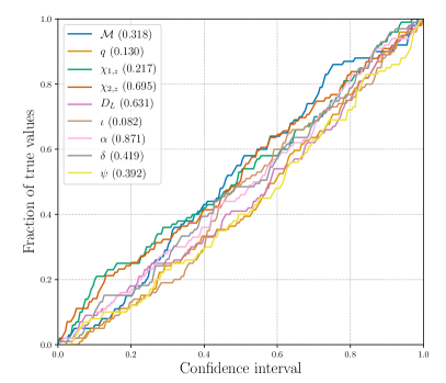
The confidence interval (CI) test has become a standard control check to verify the reliability of a GW pipeline (e.g. Veitch et al., 2015; Del Pozzo et al., 2018; Romero-Shaw et al., 2020), since it ensures that the recovered probability distributions are truly representative of the inferred confidence levels. For each parameter employed in the analyses, the CI test measures the fraction of true values that follow below a given credible level and, if the algorithm is well-calibrated, we expect this two quantities to be proportional. The test is performed using a large set of injected signals with parameters extracted from a population prior $\mathfrak{p}(\bm{\theta}_{\rm cbc})$. Then, we conduct PE analyses in order to recover the posterior distributions for every injection and the CIs can be estimated from the posterior distributions by determining the quantiles under which the true parameters lie. Then, the population prior $\mathfrak{p}(\bm{\theta}_{\rm cbc})$ is used as input prior distribution for the analysis of the injected signal .

For our CI test, we inject 100 BBH signals employing the prior distribution used for the parameters of GW150914 (see Sec. VII.1), that includes 9 parameters. The signals are generated using MLGW waveform template and injected in the two LIGO detectors, H1 and L1, at design sensitivity using segments of duration 8 s. The analyzed frequency range goes from 20 Hz to 1 kHz. We use the nested sampling provided by dynesty with 1024 live points and tolerance equal to 0.1. The likelihood function is marginalized over reference phase and time shift. Figure 10 shows the recovered fractions of events found within an increasing confidence level. The fraction of event is expected to be uniformly distributed if the prior distributions is a good approximation of the underlying injected population distributions.

For each parameter, we compute the $p$-value of Kolmogorov-Smirnov (KS) test, quantifying the consistency with uniformly distributed events. The results are shown between round brackets in Figure 10. From these results, we estimate the combined $p$-values quantifying the probability that the individual $p$-values are extracted from a uniform distribution. We estimate an overall $p$-value of $58\%$, according with analogous computations performed with a set of 9 random uniformly-distributed samples. Furthermore, we compute the Jensen-Shannon (JS) divergence between the distribution of fraction of events with respect to a uniform distribution. The results lie around $2\times 10^{-3}$ for all the parameters, in agreement with analogous estimations performed on a set of 100 uniformly-distributed random samples. These results confirm that the pipeline is well-calibrated.

VII LIGO-Virgo transients

In this section, we apply the bajes pipeline to the GW transients Abbott et al. (2019a) observed by the LIGO-Virgo interferometers Abbott et al. (2018b); Aasi et al. (2015); Acernese et al. (2015). For all the analyses, the data are extracted from the GWOSC archive Abbott et al. (2019d); Trovato (2020); LIGO Scientific and Virgo Collaboration (a) with a sampling rate of 4096 Hz resorting to the gwpy facilities. The analyzed strains are centered around the nominal GPS time. Subsequently, the strains are windowed and transformed in the Fourier space, using the tools described in Sec. IV. PSD curves and calibration uncertainties are taken from the official LIGO-Virgo data release of GWTC-1 Abbott et al. (2019a); LIGO Scientific and Virgo Collaboration (b, c). We use the nested sampling implemented in dynesty, employing 2048 live points with a tolerance equal to 0.1. With these settings, we collect ${\sim}5\times 10^{4}$ samples from each PE analysis. The measured quantities reported in the text correspond to the median values and to the 90% credible regions, except when explicitly mentioned.

We note that the prior assumptions employed in bajes slightly differs from the ones of the official LIGO-Virgo analysis. In the latter, the sampling is performed imposing additional bounds in the mass components Abbott et al. (2016a, c, 2017b, 2018a); while, in bajes, the samples are extracted from the entire square defined by the $\{\mathcal{M},q\}$ bounds. Moreover, the strains analyzed by the bajes pipeline are slightly shifted in time with respect the official LIGO-Virgo segments due to different reference conventions.

VII.1 GW150914

Figure 11: Waveform template reconstructed from the analysis of GW150914 wit TEOBResumS compared with the LIGO-Hanford (top panel) and LIGO-Livingston (bottom panel) data. The black lines are the whitened strains recorded by the LIGO inteferometers, where we applied a band-pass filter in the frequency window $[20~{}{\rm Hz},480~{}{\rm Hz}]$ only for visualization purposes. The colored lines are the median recovered template projected on the respective detector (orange for LIGO-Hanford and green for LIGO-Livingston) and the shadowed areas represents the 90% credible regions. The estimated network SNR of the signal corresponds to 22.

Figure 12: Posterior distributions for the intrinsic (left) and extrinsic (right) parameters of GW150914 estimated with bajes pipeline employing TEOBResumS waveform model with aligned spin components. All higher-order modes up to $\ell=5$ (with $m=\pm\ell$) have been used to generate the waveform models. The chirp mass is expressed in Solar masses ${\rm M_{\odot}}$, the luminosity distance is expressed in megaparsec Mpc, while the angles $\{\iota,\alpha,\delta\}$ are in radiants. We report the median value and the 90% credible regions for each parameter and the contours represent the 50% and the 90% credible regions.

In this section, we discuss the results obtained from the analysis of the first GW transient observed by the LIGO interferometers, GW150914 Abbott et al. (2016a, d, b, e). For all the discussed cases, the analyzed strains correspond to the GWTC-1 release Abbott et al. (2019a) of LIGO-Hanford and LIGO-Livingston data centered around GPS time 1126259462 with a sampling rate of 4096 Hz and a duration of 8 s. We set the lower cutoff-frequency to 20 Hz and the highest frequency to 1 kHz. The employed prior is isotropic in spin components and volumetric in luminosity distance, and it spans the ranges $\mathcal{M}\in[12,45]~{}{\rm M_{\odot}}$, $q\in[1,8]$, $\chi_{1,2}\in[0,0.99]$ and $D_{L}\in[100,5000]~{}{\rm Mpc}$. We include 8 spectral nodes for the calibrations of the analyzed strains.

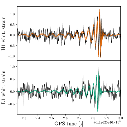
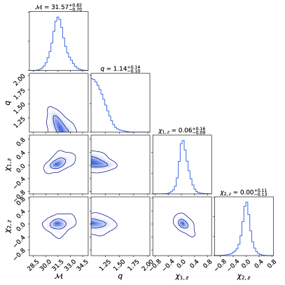
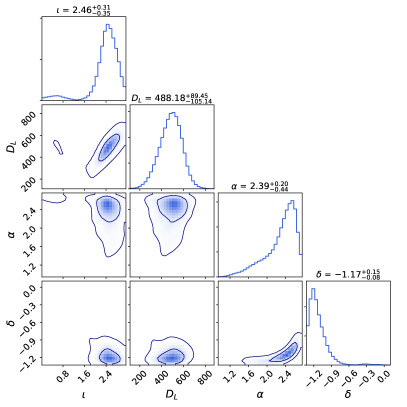
We discuss first the PE analysis employing TEOBResumS model with aligned spins, including all high-order modes up to $\ell=5$ with $m=\pm\ell$, i.e. $(2,\pm 2)$, $(3,\pm 3)$, $(4,\pm 4)$, $(5,\pm 5)$. Figure 11 shows the recovered waveform template compared with the whitened strains recorded by the LIGO interferometers, and Figure 12 shows the recovered posterior distribution. We estimated a network SNR of 23. The results are consistent with similar studies performed with the same approximant Nagar et al. (2018, 2020b), recovering the signal of a non-spinning equal-mass BBH merger with $\mathcal{M}=31.57^{+0.82}_{-0.70}~{}{\rm M_{\odot}}$. The inference of the extrinsic parameters shows a source located at a luminosity distance of ${\sim}490~{}{\rm Mpc}$ and the area covered by the 90% isoprobability level of the sky location posterior distributions corresponds to ${\sim}670~{}{\rm deg}^{2}$. The estimated Bayes' factor corresponds to $\log\mathcal{B}^{\rm S}_{\rm N}=267.8\pm 0.2$, where the uncertainty is given by the standard deviation.

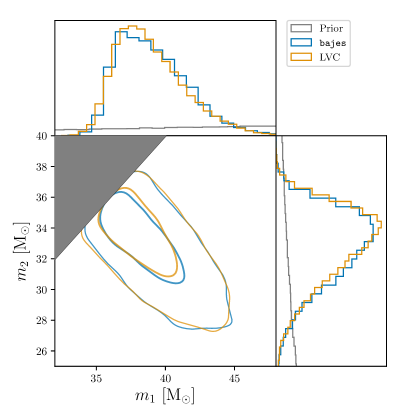
We repeat the PE analysis with IMRPhenomPv2 template employing precessing spin components. In Figure 13, the marginalized posterior distribution of the recovered masses is compared with the official LIGO-Virgo posterior samples release with GWTC-1 Abbott et al. (2019a) performed the LALInference routines Veitch et al. (2015); LIGO Scientific Collaboration (2018a) using the same waveform approximant. The two analyses are consistent with each other, recovering a BBH signal with chirp mass $\mathcal{M}=31.00^{+1.52}_{-1.49}~{}{\rm M_{\odot}}$ and mass ratio well constrained around the equal mass case, $q=1.18^{+0.36}_{-0.17}$. The inference of the effective spin parameter is consistent with zero and the posterior distribution of the spin components does not show evidence of precession, according to Ref. Abbott et al. (2016c, b, d). Also the extrinsic parameters show an overall good agreement with previous estimations performed with the same approximant, locating the source at a luminosity distance of $D_{L}=458^{+123}_{-169}$ Mpc with a posterior sky-location area of ${\sim}640~{}{\rm deg}^{2}$ at the 90% credible level.

The main difference between the TEOBResumS posterior and IMRPhenomPv2 one is the uncertainty on the mass ratio parameter, for which TEOBResumS admits a largest value of $1.28$ at the 90% credible region, while the IMRPhenomPv2 posterior reaches $1.94$ with the same confidence. However, this disagreement is mainly due to the different spin assumptions employed for the two analyses Abbott et al. (2016c, b). Moreover, the posterior distribution recovered with IMRPhenomPv2 shows slightly smaller $\mathcal{M}$ and larger $D_{L}$ compared with the TEOBResumS inference, as shown also in Ref. Nagar et al. (2018).

Figure 13: Posterior distributions of the detector-frame mass components $\{m_{1},m_{2}\}$ recovered in analysis of GW150914 with IMRPhenomPv2 (blue line). The results are compared with the official LIGO-Virgo posterior samples released with GWTC-1 Abbott et al. (2019a) (yellow line) computed using the LALInference routines Veitch et al. (2015); LIGO Scientific Collaboration (2018a). The central panel shows the 50% and the 90% credible regions.

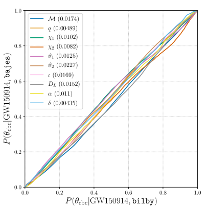
Finally, we verify the compatibility of the recovered posterior distribution against of existing GW pipelines. In particular, we employ the bilby pipeline Ashton et al. (2019); Smith et al. (2020); Romero-Shaw et al. (2020) in order to estimate the posterior distributions of GW150914, using the same prior assumptions and settings discussed above. We observe that GW150914 is a suitable candidate to test the statistical significance of the results and the agreement between the pipelines: due to the loudness of this event (corresponding to an SNR $>20$), the overall impact of statistical noise fluctuations on the recovered posterior distribution is expected to be less determinant compared with the other BBH mergers presented in GWTC-1 Abbott et al. (2019a). Figure 14 shows the probability-probability (PP) plot of the marginalized posterior distributions recovered for every parameter. A PP plot compares the cumulative distributions estimated with two methods, plotting one against the other. Then, if two probability distributions are identical, the associated PP plot is represented by a bisector line. In our case, the results coming from the two pipelines are largely consistent between each other, with observed deviation fully consistent with statistical fluctuations. This fact is confirmed by the $p$-values computed between the marginalized distributions of each parameter: the values are comparable to or larger than $0.4$ except for $\vartheta_{2}$ and $D_{L}$ parameters, for which we respectively get $p$-values of 0.15 and 0.11. Furthermore, the legend in Figure 14 shows the square root of the JS divergence of the marginalized posterior distributions for the employed parameters: the largest recovered value corresponds to $5.2\times 10^{-4}$ bit for the tilt angle $\vartheta_{2}$.

Figure 14: PP plot for the marginalized posterior distributions of GW150914 parameters. On the $x$-axis, the cumulative posterior probabilities estimated with the bilby pipeline and on the $y$-axis the same quantities computed with the bajes pipeline. Different colors refer to different parameters and the legend shows also the square root of the Jensen–Shannon divergence.

VII.2 GW170817

Figure 15: Posterior distributions for the intrinsic (left) and extrinsic (right) parameters of GW170817 estimated with bajes pipeline employing TEOBResumSPA waveform model with aligned spin components. The chirp mass is expressed in Solar masses ${\rm M_{\odot}}$, the luminosity distance is expressed in megaparsec Mpc, while the angles $\{\iota,\alpha,\delta\}$ are in radiants. We report the median value and the 90% credible levels for each parameter and the contours represent the 50% and the 90% credible regions.

Figure 16: Posterior distributions for the intrinsic parameters of GW170817 estimated with bajes pipeline employing TaylorF2 (5.5PN + 7.5PN) waveform model with aligned spin components. The chirp mass is expressed in Solar masses ${\rm M_{\odot}}$. We report the median value and the 90% credible levels for each parameter and the contours represent the 50% and the 90% credible regions.

Figure 17: Posterior distributions for the reduced tidal parameter ${\tilde{\Lambda}}$ of GW170817 estimated using the bajes pipeline with different waveform approximants and different upper cutoff-frequencies. The posterior samples has been reweighted to uniform prior distribution and the plot shows the original employed prior (gray line). Solid lines refer to the results with $f_{\rm max}=2~{}{\rm kHz}$, while dashed lines are estimated with $f_{\rm max}=1~{}{\rm kHz}$. TEOBResumSPA (blue line) and TaylorF2 (yellow line) samples are computed employing aligned spins, while precessing spin components were included for IMRPhenomPv2_NRTidal (green line).

Figure 18: Comparison between the posterior distributions for the tidal parameters $\{{\tilde{\Lambda}},{\delta\tilde{\Lambda}}\}$ estimated with the bajes pipeline (blue lines) with the official LIGO-Virgo released samples Abbott et al. (2019e) (yellow lines) computed with the LALInference routines Veitch et al. (2015); LIGO Scientific Collaboration (2018a). The analyses are performed with IMRPhenomPv2_NRTidal waveform approximant. The left panel shows the results with low-spin prior ($\chi_{\rm max}=0.05$), while the right panel presents the high-spin prior results ($\chi_{\rm max}=0.89$)s. For both panels, the central plots show the 50% and 90% credible regions. We estimate the JS divergences for the marginalized distributions, finding the values of $8.9\times 10^{-5}$ bit and $5.3\times 10^{-5}$ bit respectively for ${\tilde{\Lambda}}$ and ${\delta\tilde{\Lambda}}$ for the high-spin prior case. Regarding the low-spin prior studies, the JS divergences correspond to $8.3\times 10^{-5}$ bit and $4.7\times 10^{-5}$ bit respectively for ${\tilde{\Lambda}}$ and ${\delta\tilde{\Lambda}}$.

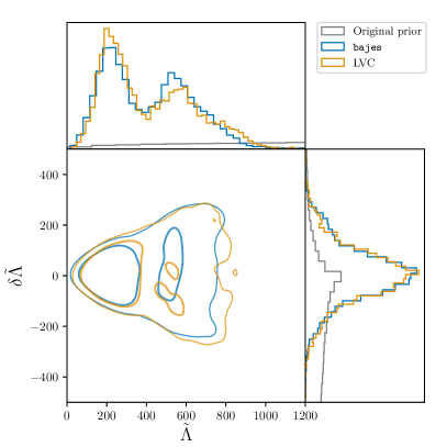
We analyze the LIGO-Virgo data corresponding to GW170817 Abbott et al. (2017b, 2018a, 2019e, 2018c), the first GW signal observed from a BNS merger. The employed data correspond to the GWTC-1 release Abbott et al. (2019a) of LIGO-Virgo data centered around GPS time 1187008857 with a sampling rate of 4096 Hz and a duration of 128 s analyzing the frequency range from 20 Hz to 2 kHz. The employed prior is isotropic in spin components and volumetric in luminosity distance, and it spans the ranges $\mathcal{M}\in[1.18,1.21]~{}{\rm M_{\odot}}$, $q\in[1,8]$, $\chi_{1,2}\in[0,0.89]$, $\Lambda_{1,2}\in[0,5000]$ and $D_{L}\in[5,75]~{}{\rm Mpc}$. We include 4 spectral nodes for the calibrations of the analyzed segments.

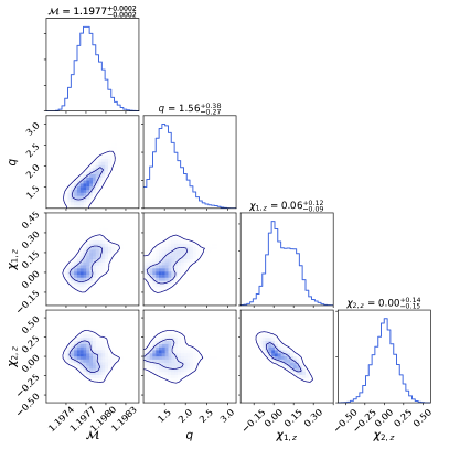
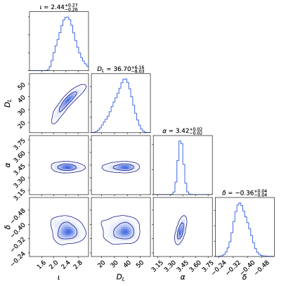
Figure 15 shows the posterior distributions for the parameters recovered employing TEOBResumSPA approximant (with $\ell=2$ and $|m|=\ell$) with aligned spins. The recovered detector-frame chirp mass corresponds to $\mathcal{M}=1.1977^{+0.0002}_{-0.0002}~{}{\rm M_{\odot}}$ and the mass ratio lies around the equal mass case, $q=1.56^{+0.38}_{-0.27}$. The spin components do not show evidence of spin contributions, consistently with Ref. Abbott et al. (2019e), with an estimated effective spin of $\chi_{\rm eff}={0.04}^{+0.06}_{-0.03}$. The primary tidal parameter $\Lambda_{1}$ is constrained to be $\lesssim 950$ at the 90% confidence level, while the secondary component $\Lambda_{2}$ is more broadly distributed over the prior. The recovered tidal parameter posterior estimates a value of ${\tilde{\Lambda}}={607}^{+477}_{-356}$, in rough agreement with previous estimations obtained from EOB models Abbott et al. (2019a); Gamba et al. (2020a). The asymmetric tidal parameter ${\delta\tilde{\Lambda}}$ shows a posterior distribution centered around non-zero values, ${\delta\tilde{\Lambda}}=92^{+200}_{-258}$; however, the hypothesis ${\delta\tilde{\Lambda}}=0$ is confidently included in the posterior support, corresponding to the $27^{\rm th}$ percentile. Moreover, the measured ${\tilde{\Lambda}}$ is overall consistent with independent estimations coming from the analysis of the EM counterpart AT2017gfo Radice et al. (2018b); Breschi et al. (2021a). Regarding the extrinsic parameters, we recovered a luminosity distance of $D_{L}=36.7^{+6.2}_{-8.0}~{}{\rm Mpc}$ and a sky location at $\{\alpha={3.42}^{+0.02}_{-0.02}~{}{\rm rad},\delta={-0.36}^{+0.04}_{-0.04}~{}{\rm rad}\}$. The estimation of the extrinsic parameters is generally consistent with previous estimations Abbott et al. (2019e, a); Gamba et al. (2020a).

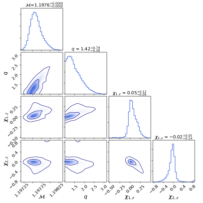
Furthermore, the analysis of GW170817 is repeated with a TaylorF2 waveform template that includes for the first time 5.5PN point-mass corrections Messina et al. (2019) and 7.5PN tidal contributions Vines et al. (2011); Damour et al. (2012). This analysis is performed using the same prior assumptions described above and the posterior distribution for the intrinsic parameters is shown in Figure 16. The mass parameters recover the values $\mathcal{M}={1.1976}^{+0.0003}_{-0.0002}~{}{\rm M_{\odot}}$ and $q=1.42^{+0.79}_{-0.36}$, while the effective spin $\chi_{\rm eff}={0.02}^{+0.07}_{-0.04}$. The estimated luminosity distance of $D_{L}={37.1}^{+10.3}_{-12.1}~{}{\rm Mpc}$. The inference of the tidal components roughly coincides with the estimations coming from the analogous analysis with PN templates Abbott et al. (2019e, a). The primary tidal component is constrained below $\Lambda_{1}<730$ at 90% credible region, while the secondary is more broadly distributed over the prior. The reduced tidal parameter is measured to be ${\tilde{\Lambda}}={404}^{+701}_{-246}$ and the asymmetric tidal term ${\delta\tilde{\Lambda}}$ is well constrained around zero with an uncertainty of ${\sim}150$ at the 90% confidence level The median values of the sky location angles coincide with the estimation performed with TEOBResumSPA.

The GW170817 PE studies are repeated with IMRPhenomPv2_NRTidal template employing precessing spin components with high-spins prior ($\chi_{\rm max}=0.89$) and low-spins prior ($\chi_{\rm max}=0.05$), in order to compare our results with the official LIGO-Virgo posterior samples presented in Ref. Abbott et al. (2019e). The recovered posterior distributions for the mass parameters for the low-spin case show a chirp mass of $1.1975^{+0.0002}_{-0.0002}~{}{\rm M_{\odot}}$ and the mass ratio is constrained below $1.46$ at the 90% credible region. Regarding the high-spin prior analysis, we recovered a chirp mass of $1.1976^{+0.0002}_{-0.0002}~{}{\rm M_{\odot}}$ and the mass ratio favors more asymmetric values, $q=1.49^{+0.35}_{-0.32}$. Focusing on the tidal parameters, Figure 18 shows the comparison of the posterior distribution in the $\{{\tilde{\Lambda}},{\delta\tilde{\Lambda}}\}$ plane: the marginalized distributions and the 90% credible regions coming from bajes are largely consistent with the official LIGO-Virgo samples, with estimated JS divergences below $10^{-4}$.

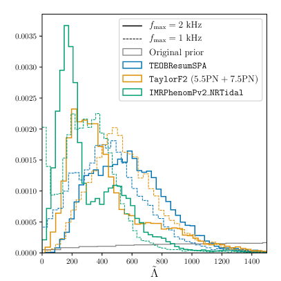
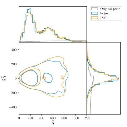
Finally, Figure 17 shows the recovered reduced tidal parameters ${\tilde{\Lambda}}$, where the posterior distributions have been reweighted to uniform prior distribution. The figure includes the results computed employing the same waveform models and using a smaller upper cutoff-frequency $f_{\rm max}=1~{}{\rm kHz}$. The main differences between the analyses with different $f_{\rm max}$ lie in the results of the tidal sector. Overall the recovered tidal parameters with $f_{\rm max}=2~{}{\rm kHz}$ appear more constrained with respect to the cases with $f_{\rm max}=1~{}{\rm kHz}$. This behavior is expected considering that the tidal information is gathered in high-frequency regimes Damour et al. (2012); Gamba et al. (2020b). On the other hand, the choice of $f_{\rm max}=2~{}{\rm kHz}$ enlarges multimodal and asymmetric behaviors in the posterior distribution of the reduced tidal parameter and systematic effects appear to be more relevant between different template families, as well known from previous studies Dai et al. (2018); Narikawa et al. (2019); Gamba et al. (2020b). The differences in the ${\tilde{\Lambda}}$ parameters can be led back to the modeling choices of the employed approximants (see Abbott et al., 2019e; Messina et al., 2019; Abbott et al., 2019a). The results estimated with TEOBResumSPA at $1~{}{\rm kHz}$ show a posterior distribution slightly shifted toward lower values with respect to the analysis at $2~{}{\rm kHz}$, consistently with what has been observed in the BNS injection study (Sec. VI.0.2). The posterior distributions for EOB and PN approximants show a good agreement with $f_{\rm max}=1~{}{\rm kHz}$.

VII.3 EOB catalog

Table 4: Prior and posterior information for the analyses of the BBH events of GWTC-1 with TEOBResumS. The GPS time refers to the central value of the time axis. For all studies, we assume aligned spins with isotropic prior. The inferred values refer to the medians of the marginalized posterior distributions and the uncertainties are 90% credible regions, except for the log-Bayes' factors $\log\mathcal{B}^{\rm S}_{\rm N}$, for which we report the standard deviations.

Data Information			Prior bounds				Inferred values
Event	GPS time	Duration	$\mathcal{M}$	$q$	$\chi_{1,2}$	$D_{L}$	$\mathcal{M}$	$q$	$\chi_{1,z}$	$\chi_{2,z}$	$\chi_{\rm eff}$	$D_{L}$	$\log\mathcal{B}^{\rm S}_{\rm N}$
	$[{\rm s}]$	$[{\rm s}]$	$[{\rm M_{\odot}}]$			$[{\rm Mpc}]$	$[{\rm M_{\odot}}]$					$[{\rm Mpc}]$
GW150914	1126259462	8	$[12,45]$	$[1,8]$	$[0,0.99]$	$[100,5000]$	${31.9}^{+1.1}_{-1.5}$	${1.20}^{+0.29}_{-0.17}$	${0.07}^{+0.39}_{-0.28}$	${0.00}^{+0.40}_{-0.42}$	${0.05}^{+0.10}_{-0.13}$	${471}^{+167}_{-231}$	$267.1^{+0.2}_{-0.2}$
GW151012	1128678900	16	$[12,45]$	$[1,8]$	$[0,0.99]$	$[100,5000]$	${18.3}^{+1.8}_{-1.0}$	${1.86}^{+2.86}_{-0.76}$	${0.05}^{+0.33}_{-0.28}$	${0.11}^{+0.53}_{-0.48}$	${0.09}^{+0.22}_{-0.17}$	${1039}^{+627}_{-626}$	$16.0^{+0.2}_{-0.2}$
GW151226	1135136350	16	$[6.5,15]$	$[1,8]$	$[0,0.99]$	$[50,5000]$	${9.71}^{+0.07}_{-0.07}$	${2.04}^{+1.59}_{-0.93}$	${0.38}^{+0.23}_{-0.24}$	${0.16}^{+0.58}_{-0.47}$	${-0.05}^{+0.45}_{-0.61}$	${490}^{+222}_{-240}$	$36.4^{+0.2}_{-0.2}$
GW170104	1167559936	16	$[12,45]$	$[1,8]$	$[0,0.99]$	$[100,5000]$	${25.6}^{+1.8}_{-2.1}$	${1.56}^{+0.86}_{-0.46}$	${0.00}^{+0.29}_{-0.32}$	${-0.04}^{+0.40}_{-0.40}$	${-0.03}^{+0.21}_{-0.25}$	${1069}^{+423}_{-446}$	$58.4^{+0.2}_{-0.2}$
GW170608	1180922494	16	$[5,10]$	$[1,8]$	$[0,0.99]$	$[50,5000]$	${8.49}^{+{0.05}}_{-{0.04}}$	${1.48}^{+{1.22}}_{-{0.42}}$	${0.06}^{+{0.30}}_{-{0.28}}$	${0.03}^{+{0.58}}_{-{0.39}}$	${0.06}^{+{0.27}}_{-{0.09}}$	${298}^{+{146}}_{-{128}}$	$80.3^{+0.2}_{-0.2}$
GW170729	1187529256	4	$[25,175]$	$[1,8]$	$[0,0.99]$	$[100,7000]$	${51.4}^{+9.1}_{-9.6}$	${1.84}^{+{0.95}}_{-{0.77}}$	${0.47}^{+{0.39}}_{-{0.48}}$	${-0.05}^{+{0.83}}_{-{0.36}}$	${0.30}^{+{0.28}}_{-{0.28}}$	${2495}^{+{1600}}_{-{1300}}$	$27.1^{+0.2}_{-0.2}$
GW170809	1185389807	16	$[12,45]$	$[1,8]$	$[0,0.99]$	$[100,5000]$	${30.3}^{+{2.3}}_{-{2.0}}$	${1.45}^{+{0.72}}_{-{0.39}}$	${0.07}^{+{0.33}}_{-{0.27}}$	${0.17}^{+{0.58}}_{-{0.21}}$	${0.17}^{+{0.24}}_{-{0.21}}$	${999}^{+{473}}_{-{483}}$	$41.8^{+0.2}_{-0.2}$
GW170814	1186302519	16	$[12,45]$	$[1,8]$	$[0,0.99]$	$[100,5000]$	${26.8}^{+{1.3}}_{-{1.0}}$	${1.29}^{+{0.52}}_{-{0.26}}$	${0.07}^{+{0.39}}_{-{0.28}}$	${0.02}^{+{0.49}}_{-{0.38}}$	${0.08}^{+{0.16}}_{-{0.12}}$	${540}^{+{224}}_{-{189}}$	$99.6^{+0.2}_{-0.2}$
GW170818	1186741861	16	$[12,45]$	$[1,8]$	$[0,0.99]$	$[100,5000]$	${31.8}^{+{3.4}}_{-{2.9}}$	${1.48}^{+{0.96}}_{-{0.43}}$	${-0.08}^{+{0.27}}_{-{0.35}}$	${0.00}^{+{0.45}}_{-{036}}$	${-0.06}^{+{0.33}}_{-{0.27}}$	${1190}^{+{594}}_{-{438}}$	$29.7^{+0.2}_{-0.2}$
GW170823	1187058327	4	$[25,175]$	$[1,8]$	$[0,0.99]$	$[100,7000]$	${37.4}^{+{5.5}}_{-{5.1}}$	${1.57}^{+{0.94}}_{-{0.51}}$	${-0.01}^{+{0.42}}_{-{0.33}}$	${0.06}^{+{0.56}}_{-{0.55}}$	${0.03}^{+{0.30}}_{-{0.28}}$	${1690}^{+{1081}}_{-{880}}$	$39.5^{+0.2}_{-0.2}$

As full scale application, we reproduce the analyses of the BBH mergers published in GWTC-1 Abbott et al. (2019a) employing the bajes pipeline and the time-domain EOB waveform model TEOBResumS, including only the dominant $(2,2)$ mode. Table 4 shows the priors used for each event, where the nominal GPS time refers to the central value of the analyzed time axis. For all the studies, the analyzed frequency range goes from 20 Hz to 1 kHz and we assume aligned spin components with isotropic prior distribution and volumetric prior for the luminosity distance. The prior distributions for the other parameters are chosen accordingly with Sec. V.2. For these studies, we employ 8 calibration envelope nodes for each detector, the phase $\phi_{0}$ is marginalized during the likelihood evaluations and the time-shift parameter $t_{0}$ is sampled from a $2~{}{\rm s}$ window centered around the nominal GPS time.

Figure 19 shows the posterior distributions marginalized in the mass components and spin magnitudes planes for all the analyzed BBH events. The mass components are expressed in the source-frame of the binaries assuming the cosmological model presented in Ref. Aghanim et al. (2020). The detector-frame mass components $m_{i}$ can be estimated in the source-frame of the binary as

$$m_{i}^{\rm src}=\frac{m_{i}}{1+z}\,,\quad i=1,2\,,$$ (43)

where $z$ is the cosmological redshift of the source. In general, the recovered mass parameters show a predominance of equal mass binaries with mass ratio well constrained below $q\lesssim 3$, except for the low-mass binary GW151012, that admits values of $q\simeq 5$ at 90% credible level. The recovered mass components are distributed between $7~{}{\rm M_{\odot}}$ and $70~{}{\rm M_{\odot}}$, with an abundance in the range $[20~{}{\rm M_{\odot}},50~{}{\rm M_{\odot}}]$. In terms of spin contributions, the most interesting events are GW151226, whose posterior distribution excludes the non-spinning case at 90% confidence level, consistently with Ref. Abbott et al. (2019a); Schmidt et al. (2020), and GW170729, which recovers an effective spin of $\chi_{\rm eff}\approx{0.3}$ and admits values up to $\chi_{1}\gtrsim 0.9$. The other GW transients show mitigated spin contributions, with $\chi_{1}\lesssim 0.5$ at the 90% credible level. Generally, the posterior distributions for the secondary spin component $\chi_{2}$ are more broadly distributed and less informative than those for the primary component $\chi_{1}$.

Furthermore, Fig. 20 shows the posterior distributions of final masses $M_{\rm f}^{\rm src}$ (estimated in the source-frame) and final spin magnitudes $\chi_{\rm f}$ expected for the merger remnants. The values are computed resorting to NR formulae presented in Ref. Jiménez-Forteza et al. (2017), calibrated with aligned-spin BBH simulations. The majority of the recovered final spins $\chi_{\rm f}$ lie around ${\sim}0.67$ due to the moderated spin contributions of the observed mergers. Regarding the extrinsic parameters, Fig. 21 shows the posterior distributions of the sky location. The sky maps for GW170814 and GW170818 show slightly larger bimodal behavior compared with the results presented in GWTC-1 Abbott et al. (2019a). On the other hand, the 90% credible region for GW170104 appears to be more constrained. Note that the aligned-spin assumption affects the overall SNR and, then, the recovered posterior distributions Dal Canton et al. (2014, 2015). The measurements for the sky locations of the other events do not show considerable deviations from the GWTC-1 estimations Abbott et al. (2019a). Fig. 22 shows the correlations of the the luminosity distance $D_{L}$ with the inclination angle $\iota$ and with the total mass $M=m_{1}+m_{2}$ (estimated in the detector frame). The luminosity distances are in agreement with the GWTC-1 estimations, while the inclination angles show slightly wider posterior supports due to the degeneracy introduced with the aligned-spins assumption Apostolatos et al. (1994).

For the GW150914 case, we can compare the analysis with higher-order modes (presented in Sec. VII.1) with the results estimated using only dominant mode. First of all, the results with $\ell\geq 5$ show narrower uncertainties, consistently with the inclusion of a larger amount of physical information Calderón Bustillo et al. (2017); Breschi et al. (2019a); Mills and Fairhurst (2021). On the other hand, the estimated Bayes' factors do not show strong evidence in favor or against the inclusion of higher-order modes, as expected for this kind of source; higher-order modes are expected to be more relevant for large mass ratios and edge-off binaries Varma et al. (2014); Calderón Bustillo et al. (2015). Overall, the median values of the recovered parameters are consistent between each other except for the mass ratio, that appears to be more constrained around $q=1$ including higher-modes.

In conclusion, we shown that TEOBResumS can be effectively applied to BBH signals, obtaining robust and consistent results Nagar et al. (2018). The main limitation of the presented results comes from the aligned-spins assumption, that introduces degeneracy with other parameters and induces biases in population inferences Stevenson et al. (2017); Farr et al. (2017); Tiwari et al. (2018). We are planning to extend the presented catalog including precessing spin terms Akcay et al. (2020) and verifying the importance of eccentric contributions Chiaramello and Nagar (2020). In terms of computational cost, TEOBResumS shows an overall good behavior, performing the analysis of a typical BBH (with length of $8~{}{\rm s}$) in ${\sim}14~{}{\rm hours}$ on 32 CPUs.

Figure 19: Marginalized posterior distribution for the source-frame mass components $\{m_{1},m_{2}\}$ (left) and the spins $\{\chi_{1},\chi_{\rm eff}\}$ (right) of the BBH mergers presented in GWTC-1 Abbott et al. (2019a). The PE studies have been performed with TEOBResumS model. The masses are expressed in the binary source-frame employing the cosmological model proposed in Ref. Aghanim et al. (2020). The contours refer to the 90% credible regions.

Figure 20: Marginalized posterior distribution for the final masses and spins $\{M_{\rm f}^{\rm src},\chi_{\rm f}\}$ for the remnants of the BBH mergers presented in GWTC-1 Abbott et al. (2019a). The analyses are performed using the bajes pipeline and TEOBResumS waveform approximant. The values have been computed from the posterior samples employing NR formulae presented in Ref. Jiménez-Forteza et al. (2017). The final masses are expressed in the source-frame of the binary. The contours refer to the 90% credible regions.

Figure 21: Marginalized posterior distribution for right ascension and declination angles $\{\alpha,\delta\}$ (represented using a Mollweide projection) for the BBH mergers presented in GWTC-1 Abbott et al. (2019a). The analyses are performed using the bajes pipeline and TEOBResumS waveform approximant. The right ascension $\alpha$ is expressed in hours, while the declination $\delta$ is reported in degrees. The contours refer to the 90% credible regions.

Figure 22: Marginalized posterior distribution for inclination angle and luminosity distance $\{\iota,D_{L}\}$ (left) and for luminosity distance and total mass $\{D_{L},M\}$ (right) for the BBH mergers presented in GWTC-1 Abbott et al. (2019a). The analyses are performed using the bajes pipeline and TEOBResumS waveform approximant. The contours refer to the 90% credible regions.

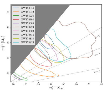
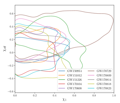
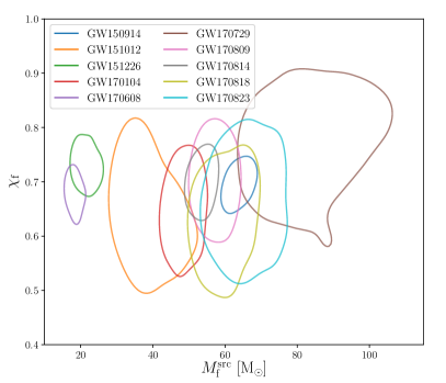
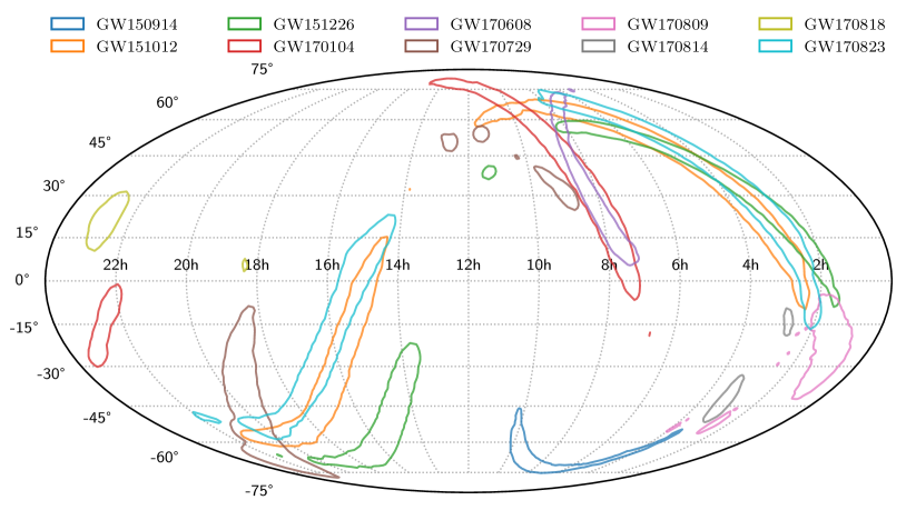
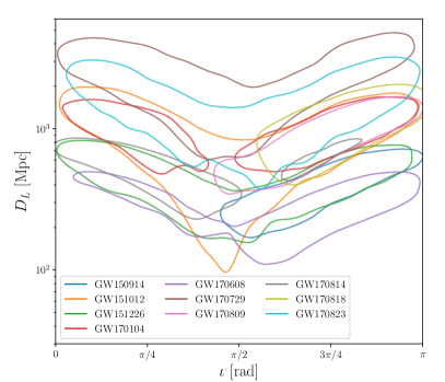
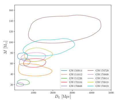
VIII Conclusion

In this paper we presented bajes, a parallel, lightweight infrastructure for Bayesian inference, whose main application is the data analysis of gravitational-wave and multimessenger transients. bajes is implemented in Python and comes with a versatile framework for Bayesian inference and different state-of-art samplers. Furthermore, it provides methods for the analysis of GW and EM transients emitted by compact binary coalescences. We benchmarked bajes by means of injection-recovery experiments with BBH merger, BNS inspiral-merger and postmerger signals. The injection studies and statistical tests show that the bajes pipeline is well calibrated and it provides robust results, within the expected statistical fluctuations.

The injections of BNS postmerger signals also offered the first detectability study with a five-detectors-network including LIGO, Virgo, KAGRA and third-generation ET Punturo et al. (2010); Hild et al. (2011). We find BNS postmerger signal will be detectable for optimally oriented sources located at ${\lesssim}80~{}{\rm Mpc}$. This result is largely merit of the ET sensitivity Punturo et al. (2010); Hild et al. (2011), that contribute to 90% of the SNR. According with recent population studies Abbott et al. (2020c) and using the distance threshold estimated from our survey with third-generation network (${\sim}$80 Mpc), the detection rate of these sources is expected to be $0.5{-}2$ events per year. As discussed in Sec. VI.0.3, the detection of such a transient, combined with the knowledge of EOS-insensitive relations, can reveal essential properties of the nuclear matter at high densities, improving significantly the EOS constraints Breschi et al. (2019b).

We demonstrated the reliability of bajes in analyzing the observational data recorded by the LIGO-Virgo interferometers Abbott et al. (2019a, d). The posterior distributions for the parameters of GW transients computed with the bajes are in agreement with the results from other GW pipelines Veitch et al. (2015); Lange et al. (2018). The direct comparison of the bajes results on GW150914 with the ones obtained with the bilby Ashton et al. (2019); Smith et al. (2020); Romero-Shaw et al. (2020) pipeline shows a maximum JS divergence of $5.2{\times}10^{-4}$ bit for the tilt angle $\vartheta_{2}$ and the marginalized posterior distributions are largely consistent between each other. Furthermore, the analyses of GW150914 with TEOBResumS approximant slightly emphasize the relevance of higher-order modes for improving the accuracy of the binary properties estimations.

We performed PE studies on GW170817 using TEOBResumSPA, IMRPhenomPv2_NRTidal and, for the fitrst time, TaylorF2 including 5.5PN point-mass contributions and 7.5PN tidal terms. The novel analysis with the extended PN model shows a good agreement with previous estimations performed with the same template family Abbott et al. (2019a, e). Using IMRPhenomPv2_NRTidal template, we found full consistency with previous results and the official LIGO-Virgo posterior samples Abbott et al. (2019a, e). Posterior distributions for the reduced tidal parameter ${\tilde{\Lambda}}$ recovered with upper cutoff-frequency $f_{\rm max}=2~{}{\rm kHz}$ show larger systematic biases between different waveform templates compared with the $1~{}{\rm kHz}$ analyses. However, using a larger $f_{\rm max}$, it is possible to take into account a larger amount of tidal information that leads to more constrained measurements. The tidal parameter ${\tilde{\Lambda}}$ estimated with TEOBResumSPA has slightly larger values compared with the measure of TaylorF2 and IMRPhenomPv2_NRTidal with $f_{\rm max}=2~{}{\rm kHz}$. The results of EOB and PN models are in overall good agreement if $f_{\rm max}=1~{}{\rm kHz}$ is employed and also with independent analysis of AT2017gfo Breschi et al. (2021a). We note that parallelization methods are key for the PE of BNS signals associated to long data segments ${\gtrsim}100\,$s. The bajes runs discussed in Sec. VII.2 were efficiently performed on 128 CPUs with total execution-time of ${\sim}$1 day.

Future work will present the validation and the application of bajes to multimessenger analyses, including EM counterparts like kilonovae and $\gamma$-ray burst (e.g. Hayes et al., 2020; Breschi et al., 2021a). Moreover, we are implementing reduced-order-quadrature Canizares et al. (2015); Smith et al. (2016); Morisaki and Raymond (2020) and the relative-binning Zackay et al. (2018); Dai et al. (2018) in order to speedup the likelihood evaluations in the GW studies. Inferences on the properties of neutron star matter will be supported with the inclusion of a parametrized EOS sampling method Read et al. (2009); Raithel et al. (2016). Moreover, future bajes releases will include an extended set of nested samplers, in particular algorithms based on machine learning (e.g. Albert, 2020) and efficiently parallelizable routines (e.g. Buchner, 2021).

bajes is publicly available at

https://github.com/matteobreschi/bajes

and contributions from the community are welcome. The posterior samples presented in Sec. VII.3 and the configuration files to reproduce the runs are available on Zenodo Breschi et al. (2021b).

Appendix A MCMC and PTMCMC

A generic Markov-chain Monte Carlo (MCMC) algorithm explores the parameter space moving forward region with increasing value of the probability and returns a set of independent samples representative of the target probability density. The MCMC samplers implemented in bajes is based on emcee Foreman-Mackey et al. (2013): this routine represents a simple and complete implementation of a Metropolis-Hastings sampling that takes advantage of parallel chains.

The MCMC algorithm can be summarized as follows. An arbitrary number of chains, say $n_{\rm chain}$, are initialized with as many random prior sample. For each chain, the last stored sample is evolved and a new sample $\bm{\theta}^{*}$ is proposed according to predefined proposal methods (see App. C). The new sample $\bm{\theta}^{*}$ is accepted with probability

$${\rm min}\left[\,1,\,\frac{p(\bm{\theta}^{*}|\textbf{d},H)}{p(\bm{\theta}_{i}|\textbf{d},H)}\,\frac{q(\bm{\theta}_{i}|\bm{\theta}^{*})}{q(\bm{\theta}^{*}|\bm{\theta}_{i})}\right]\,,$$ (44)

where $\bm{\theta}_{i}$ is the last sample of the chain and $q(\bm{\theta}_{i}|\bm{\theta}_{j})$ is the proposal density function computed between $\bm{\theta}_{i}$ and $\bm{\theta}_{j}$. This procedure is iterated for every chain of the ensemble and samples are collected during the exploration. Note that, according with prescription Eq. (44), the probability of the proposed sample is not required to be strictly greater than that of the current sample. The initial exploration is called burn-in, in which the chains randomly explores the surrounding prior volume. The algorithm spends these iterations in order to localize the maximum-probability region. After a certain amount of iterations, depending on the complexity of the parameter space, the chains can converge and the actual collection of posterior samples starts. Subsequently, when the algorithm reaches the stopping condition, the burn-in portion is removed, the samples from different chains are joined together, the autocorrelation length (ACL) is computed in order to estimate the effective number of independent posterior samples, and the final set of samples is extracted from the joined set according with the value of ACL. The stopping criterion implemented in bajes for the MCMC algorithms is defined by the requested number of output samples $n_{\rm out}$,

$$\frac{\left(i-n_{\rm burn}\right)\,n_{\rm chain}}{{\rm ACL}}\geq n_{\rm out}\,,$$ (45)

where $i$ is the current iteration, $n_{\rm chain}$ is the total number of chains, $n_{\rm burn}$ is the number of iterations required for burn-in and ACL is computed on the set of post-burn-in samples .

The MCMC algorithm disposes of a light-weighted settings and it is a fast and versatile algorithm. However, when the parameter space becomes large or the distributions have multimodalities, this method could have many issues; such as insufficient and inaccurate exploration of the parameter space, some chains could get trapped in a local minima or the ensemble might not be able to reach convergence. These issues can be mitigated resorting to a large number of parallel chains or to specific proposal methods (see App. C). Moreover, given a set of posterior samples, it is possible to estimate the evidence using the approximation

$$p(\textbf{d}|H)\approx\frac{1}{n_{\rm samples}}\sum_{i=1}^{n_{\rm samples}}p(\bm{\theta}_{i}|\textbf{d},H)\,,$$ (46)

where the index $i=1,\dots,n_{\rm samples}$ runs over the posterior samples. However, in general, Eq. (46) is unable to perform accurate estimations of the evidence, since the MCMC algorithm is not designed to minutely inspect all the parameter space.

On the other hand, the parallel tempering MCMC (PTMCMC) Earl and Deem (2005); Swendsen and Wang (1986); Neal (1996) performs improved exploration of the parameter space and it provides a more accurate estimations of the evidence integral compared to standard MCMC techniques. The PTMCMC sampler implemented in bajes is inspired by ptemcee Vousden et al. (2015). The PTMCMC introduces an inverse temperature coefficient $\beta=1/T\in[0,1]$ in the computation of posterior distribution, such that

$$p_{\beta}(\bm{\theta}|\textbf{d},H)\propto\big{[}p(\textbf{d}|\bm{\theta},H)\big{]}^{\beta}p(\bm{\theta}|H)\,.$$ (47)

The set of all chains is grouped in equally-populated sub-ensembles and a different value of $\beta$ is associated to each tempered ensembles. The default $\beta$ ladder is geometrically-spaced in the range $[0,1]$. The algorithm proceeds as the usual MCMC for every chain using the tempered posterior distribution Eq. (47). For $T=1$, the tempered posterior is identical to the original one and low-temperature chains will move toward regions with large likelihood values focusing on the estimation of the volume of the bulge. However, the contribution of the likelihood function is mitigated by increasing values of $T$, up to the limit $T\to\infty$, where the posterior is identically equal to the prior. Then, high-temperature chains will be able to freely explore the majority the prior support, inspecting the tails of the targeted posterior distribution and providing a good coverage of the entire prior volume. Furthermore, the algorithm proposes swaps between consecutive pairs of chains, received with acceptance

$${\rm min}\left[\,1,\,\left(\frac{p(\textbf{d}|\bm{\theta}_{i},H)}{p(\textbf{d}|\bm{\theta}_{j},H)}\right)^{\beta_{j}-\beta_{i}}\right]\,,$$ (48)

where $\bm{\theta}_{i}$ and $\beta_{i}$ are respectively the last sample and the inverse temperature of the $i$-th chain, and analogously for $j$. If the swap is accepted the position of the two samples are exchanged in the different selected chains. This procedure allows the information of the high-temperature chains to propagate to the low-temperature ones and viceversa, improving the correlation between the samples. Another key feature of parallel tempering is that it satisfies the detailed balance condition Sambridge (2013), required for convergence of the MCMC chains.

Finally, the stopping criterion Eq. (45) is estimated for the untempered chains; when it is satisfied, the sampler stops and reproduces the posterior samples using only the chains of the $T=1$ sub-ensemble. Furthermore, using the auxiliary coefficient $\beta$ and thermodynamic integration Goggans and Chi (2004); Lartillot and Philippe (2006), it is possible to write the evidence as

$$\log p(\textbf{d}|H)=\int_{0}^{1}E_{\beta}\big{[}\log p(\textbf{d}|\bm{\theta},H)\big{]}\,\text{d}\beta\,.$$ (49)

where the expectation value is estimated using the tempered posterior, i.e.

$$E_{\beta}\left[f(\bm{\theta})\right]=\int_{\bm{\Theta}}f(\bm{\theta})\,\big{[}p(\textbf{d}|\bm{\theta},H)\big{]}^{\beta}p(\bm{\theta}|H)\,\text{d}\bm{\theta}\,.$$ (50)

Eq. (49) can be estimated through numerical integration. The terms $E_{\beta}\left[\log p(\textbf{d}|\bm{\theta},H)\right]$ are estimated over the initial $\beta$ ladder applying Eq. (46) to the tempered posterior samples and the integral is approximated using the trapezoidal rule. The PTMCMC represents an improved version of a standard MCMC technique, that aims to provide much accurate estimations of the evidence. However, the accuracy of the estimation Eq. (49) strongly depends on the number of employed temperatures: in complex situations, the total number of chains needed to accurately estimate the evidence could overcome the number of available processes, affecting the efficiency of the sampler Gupta et al. (2018).

Appendix B Nested sampling

The nested sampling Skilling (2006); Sivia and Skilling (2006) is a finely-designed Bayesian technique designed to accurately estimate the evidence integral and, nevertheless, it provides a set of posterior samples as final product of the algorithm. The strength of this technique is the capability to succeed even in cases of high-dimensional parameter space or multimodal distributions. Nested sampling computes the evidence identifying nested isoprobability contours and estimating the amount of prior volume enclosed by each level. The main advantage of this technique is the reduction of the multidimensional integral Eq. (2) to a one-dimensional problem Chopin and Robert (2010); Betancourt et al. (2011), introducing the variable

$$X(\lambda)=\int_{p(\textbf{d}|\bm{\theta},H)>\lambda}p(\bm{\theta}|H)\,\text{d}\bm{\theta}\,.$$ (51)

The quantity $X(\lambda)$ is usually labeled as prior mass and it is the cumulative prior volume covering all likelihood values greater than $\lambda$. The prior mass takes values in the range $[0,1]$, where $X=1$ corresponds to the entire prior volume. Then, we can rewrite the likelihood as function of the prior mass, i.e. $p(\textbf{d}|X(\lambda),H)=\lambda$, from which follows,

$$p(\textbf{d}|H)=\int_{0}^{1}p(\textbf{d}|X,H)\,\text{d}X\,.$$ (52)

Eq. (52) has a further advantage: by definition, the likelihood $p(\textbf{d}|X,H)$ is a monotonic decreasing function of $X$. Then, for $X\to 0$, the likelihood tends to its maximum value. Accomplishing the transformation $\bm{\theta}\to X$ involves dividing the unit prior mass range into small bins and sorting them by likelihood.

A standard nested sampling routine requires an input number of live points $n_{\rm live}$ and a real positive number $\zeta$ representing the final tolerance of the computation. The live points are samples of the parameter space that are evolved during the routine: starting from a set of $n_{\rm live}$ initial samples (usually extracted from the prior distribution), the live point with lowest likelihood value, say $\bm{\theta}_{i}$, is discarded and replaced with a new point $\bm{\theta}^{*}$ extracted from the prior distribution that satisfies the relation $p(\textbf{d}|\bm{\theta}^{*},H)>p(\textbf{d}|\bm{\theta}_{i},H)$. The new point $\bm{\theta}^{*}$ is usually proposed using internal MCMC routines (see App. C). The procedure is repeated taking the lowest-likelihood live point at every iteration, such that the algorithm starts inspecting the entire prior volume ($X_{0}=1$), and it moves toward lower value of the prior mass,

$$0<X_{i}<\dots<X_{2}<X_{1}<X_{0}=1\,,$$ (53)

up to the the most likely value(s), where the majority of the likelihood volume is located. At the $n$-th iteration, the evidence is approximated from Eq. (52) using trapezoidal rule,

$$p_{n}(\textbf{d}|H)\approx\frac{1}{2}\sum_{i=1}^{n}\left(X_{i-1}-X_{i+1}\right)\,p(\textbf{d}|\bm{\theta}_{i},H)\,,$$ (54)

where $X_{i}$ is estimated with the expectation value Betancourt et al. (2011),

$$E[X_{i}]=e^{-i/n_{\rm live}}\,.$$ (55)

From Eq. (55), we can deduce that the average volume occupied by a live point corresponds to the $n_{\rm live}$-th part of the current prior mass. Then, increasing $n_{\rm live}$, the sampling will perform a finer grained inspections of the prior volume. In the nested sampling context, the $i$-th extracted sample is taken as representative element of the respective isoprobability level of likelihood and, since the algorithm accepts strictly increasing likelihood values, it ensures that each level is nested in the previous one. Then, the overall evidence is computed summing all the likelihood contributions from each nested level weighted on the expected difference in prior mass, according with Eq. (55). The specific stopping condition depends on the requested sampler. In general, if the algorithm converged to the global maximum-likelihood value, at the $n$-th iteration the evidence is expected to vary at most of

$$\Delta_{n}=\max_{i\leq n}\big{[}p(\textbf{d}|\bm{\theta}_{i},H)\big{]}\cdot X_{n}\,,$$ (56)

where $\max_{i\leq n}[p(\textbf{d}|\bm{\theta}_{i},H)]$ is the maximum likelihood discovered up to the $n$-th iteration. Then, the general stopping criterion requires that the estimated evidence is not expected to change more than a factor $e^{\zeta}$, i.e.

$$\zeta\geq\log\left(1+\frac{\Delta_{n}}{p_{n}(\textbf{d}|H)}\right)\,.$$ (57)

When the stopping condition is satisfied, the sampler stops and it includes the contributions of the remaining live points to the overall evidence. Then, the posterior distribution can be reconstructed by the chain of collected samples, weighting each point according with its probability distribution,

$$p(\bm{\theta}_{k}|\textbf{d},H)\approx\frac{\left(X_{k-1}-X_{k+1}\right)}{2}\,\frac{p(\textbf{d}|\bm{\theta}_{k},H)}{p(\textbf{d}|H)}\,,$$ (58)

where the index $k$ runs over the extracted samples Hol et al. (2006).

The nested sampling routine offers a much better architecture for evidence estimation than MCMC techniques. In general, the estimated log-evidence carries a statistical uncertainty inversely proportional to $n_{\rm live}$ due to the marginalization over the prior mass; while, numerical errors are dominated by the use of point estimates and by the length of the MCMC sub-chains $n_{\rm MCMC}$ used to propose new samples, as shown in Ref. Veitch and Vecchio (2010). This inefficiency can be suppressed estimating the ACL of the MCMC sub-chains and proposing a new sample independent of the previous one. Note that also the estimation of the posterior samples Eq. (58) is affected by statistical and numerical uncertainty Higson et al. (2018).

The cpnest Pozzo and Veitch software represents an exemplary implementation of a standard nested sampling: the code is designed to be nicely interfaced with user-defined models and its sampling methods can be easily customized. On the other hand, dynesty Speagle (2020) takes advantage of flexible bounding methods Buchner (2014, 2017), that aim to define isoprobability contours in order to exclude least likely regions of the parameter space improving the robustness of the algorithm. Moreover, dynesty provides an implementation of dynamic nested sampling Higson et al. (2019): this technique allocates an adaptive number of live points at each iteration iteration $i$, i.e. $n_{\rm live}\equiv n_{\rm live}(i)$. Since the change in prior volume at a given iteration depends on the number of live points, as shown in Eq. (55), the possibility of varying $n_{\rm live}$ gives the algorithm the freedom to control the effective resolution of the sampling as a function of prior mass, adapting it to the shape of the posterior in real time and improving the evaluation of the posterior density. Since the architecture of the dynamic nested sampling differs from the standard, it requires modified methods in order to compute the evidence and estimate the posterior. By default, the importance of each sample for the evidence computation is proportional to the amount of the posterior density enclosed in the prior mass probed by that point.

Appendix C Proposal methods

The exploration of the parameter space is defined by proposal methods which aim to move a sample toward a more likely position in the parameter space independent from the previous. The efficiency of the proposals determines the rate of acceptance of new samples and it affects the final ACL and subsequently the efficiency of the whole sampler. It follows that these tools are fundamental for the chains progress and a generic, broad and varied combination of proposal methods is needed to accurately inspect the entire parameter space. For this reason, bajes implements an assorted combination of proposal methods.

Before discussing the specific proposals implemented in bajes, we observe that a generic proposal method requires the introduction of a proposal distribution $q$, in order to satisfy the detailed balance. A proposal distribution $q(\bm{\theta}^{*}|\bm{\theta}_{i})$ quantifies the probability of proposing $\bm{\theta}^{*}$ given $\bm{\theta}_{i}$. A symmetric proposal is such that the proposed point is fully independent from the initial sample, i.e. $q(\bm{\theta}^{*}|\bm{\theta}_{i})\propto 1$ for every $(\bm{\theta}^{*},\bm{\theta}_{i})$. The interested reader might look at Ref. Hastings (1970); Roberts and Rosenthal (2007) for details on Markovian process.

• Prior proposal: A new point is extracted from the prior distribution generating a sample uniformly distributed over an hyper-cube and projecting it in the current parameter space according with the prescribed prior. This method could show low acceptance on long-time scales, especially for complex posterior distribution. However, it can improve the exploration of the parameter space and it does not require expensive computations.

• Stretch proposal: This method is introduced in Ref. Goodman and Weare (2010) and it make use of an auxiliary random sample $\bm{\theta}_{a}$ extracted from the history of the chains. A new sample $\bm{\theta}^{*}$ is proposed from the initial position $\bm{\theta}_{i}$ according with

  $$\bm{\theta}^{*}=\bm{\theta}_{a}+\xi\,(\bm{\theta}_{i}-\bm{\theta}_{a})\,.$$ (59)

  where $\xi$ is a scale factor. As pointed out in Ref. Christen and Fox (2010), this proposal is symmetric if the probability density of scaling factor $g(\xi)$ satisfy the condition $g(1/\xi)=\xi\,g(\xi)$. The bajes implementation adopts the settings presented in Ref. Foreman-Mackey et al. (2013). In order to satisfy the detailed balance, this proposal method requires an acceptance factor,

  $$\frac{q(\bm{\theta}_{i}|\bm{\theta}^{*})}{q(\bm{\theta}^{*}|\bm{\theta}_{i})}=\xi^{n_{\rm dim}-1}\,,$$ (60)

  where $n_{\rm dim}$ is the number of dimensions of the parameter space. Eq. (60) is computed conditioning of the target distribution on the trajectory described by Eq. (59). The method shows a good adaptation to arbitrary shapes of the distributions Goodman and Weare (2010) but it might become inefficient for multimodal cases.

• Random walk proposal: This method is introduced in Ref. Goodman and Weare (2010). The new sample $\bm{\theta}^{*}$ is extracted from a multivariate normal distribution, centered in the initial sample $\bm{\theta}_{i}$ and with covariance defined using a subset of $N$ auxiliary points randomly extracted from the history of the chains. By default, bajes walk proposal uses $N=25$. This symmetric method is efficient with unimodal distributions and it can improve the correlation between the samples. However, it becomes inefficient in case of complex posterior distribution since it is not capable to arbitrarily adapt its shape.

• Replacement proposal: This method is introduced in Ref. Goodman and Weare (2010). A subset of $N$ auxiliary points $\bar{\bm{\Theta}}\equiv\{\bar{\bm{\theta}}_{k}\}$ is randomly chosen from the history of the chains and it is used to identify a probability distribution $p(\bm{\theta}|\bar{\bm{\Theta}})$ from which the new samples will be extracted. The idea is to estimate $p(\bm{\theta}|\bar{\bm{\Theta}})$ such that is it capable to approximate the target distribution, increasing the acceptance. Moreover, the estimation can be refined and adapted during the exploration of the parameter space. In order to estimate $p(\bm{\theta}|\bar{\bm{\Theta}})$, the replacement proposal implemented in bajes employs a Gaussian kernel density estimation with $N=25$. However, this method does not access to unexplored regions of the parameter space, with the possibility of leading to highly correlated chains. Furthermore, this method is not symmetric and the proposal distribution is described by $p(\bm{\theta}|\bar{\bm{\Theta}})$.

• Differential evolution proposal: This method is introduced in Ref. Nelson et al. (2013) and it aims to solve problems due to multimodal distributions using a differential move based on the information on the explored samples. Two auxiliary random samples $\{\bm{\theta}_{a,b}\}$ are extracted from the from the history of the chains and a new sample $\bm{\theta}^{*}$ is proposed from $\bm{\theta}_{i}$ as

  $$\bm{\theta}^{*}=\bm{\theta}_{i}+\gamma\left(\bm{\theta}_{a}-\bm{\theta}_{b}\right)\,,$$ (61)

  where $\gamma$ is a scale factor whose value is randomly extracted when a new sample is proposed. The differential evolution proposal of bajes assign $\gamma=1$ with 50% of probability in order to to improve the mixing between different modes. The remaining 50% ot the time, the scale factor is extracted from a normal distribution such that $\gamma\sim{\rm N}(0,2.38/\sqrt{2n_{\rm dim}})$, where $n_{\rm dim}$ is the dimension of the parameter space. This choice has been proved to increase the acceptance of the algorithm DEp ; Roberts and Rosenthal (2001). In general, differential evolution is capable to capture linear correlations and improve mixing between different modes, however it can perform poorly in more complicated scenarios.

• Eigenvector proposal: This method computes the covariance from history of the chains and estimates the relative eigenvectors. Then, the new point is proposed moving the initial sample along a random eigenvector of the covariance with a scale prescribed by the respective eigenvalue. As shown in Ref. Veitch et al. (2015), this method can improve the efficiency of the sampler and decrease the correlation of the chains.

• Ensemble slice proposal: This method has been introduced in Ref. Karamanis and Beutler (2020) and it represents an ensemble-based improvement of the standard slice proposal Neal (2003). Let us call $\bm{\theta}_{i}$ and $p_{i}$ respectively the initial sample and its probability. The method extracts a value $y\sim{\rm U}(0,p_{i})$ and estimates a direction in the parameter space $\bm{\eta}$, resorting to the information of the ensemble samples and using differential and Gaussian estimations. Then, the initial sample is moved along the slide defined by the direction $\bm{\eta}$ and a new point $\bm{\theta}^{*}$ is proposed when the associated probability value $p^{*}$ is greater than $y$. With respect to standard slice sampling Neal (2003), this method takes advantage of adaptive scale factors refined during the evolution of the sampler that increase the efficiency of the proposal and drastically reduce the correlation between the collected samples. On the other hand, the ensemble slice proposal requires multiple likelihood evaluations; then, when the likelihood is computationally expensive, it might affect the computational cost of the whole algorithm.

• GW-targeted proposal: As discussed in Ref. Veitch and Vecchio (2010); Veitch et al. (2015), generic posterior distributions of GW signal parameters show many multimodalities and large correlations between different parameters. Moreover, its shape is usually elongated and non-regular. Then, in order to properly and efficiently explore the parameter space, it is useful to inform the proposal method with known structures expected in the posterior distributions and it is possible to take advantage of the determined analytical dependencies on the extrinsic parameters. The GW-targeted proposal implemented in bajes explores most of the GW specific methods introduced in Ref. Veitch and Vecchio (2010); Veitch et al. (2015); such as sky reflection, Gibbs sampling for the luminosity distance, and specific methods to explore the phase-polarization and the distance-inclination correlations.

Appendix D Simple example

Figure 23: Posterior distribution for the parameters $\{\theta_{1},\theta_{2},\theta_{3}\}$ discussed in App. D. The blue lines correspond to the results obtained with PTMCMC sampler, while the yellow and green lines refer respectively to cpnest and dynesty results. The marginalized contours are the 50% and 90% credible regions.

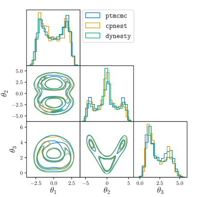
In this section we show a simple example of Bayesian inference performed with the samplers implemented in bajes. We use a 3-dimensional parameter space $\bm{\theta}=\{\theta_{1},\theta_{2},\theta_{3}\}$ bounded to $\theta_{i}\in[-8,+8]$ for $i=1,2,3$ with an uniformly distributed prior distribution. For the sake of simplicity, we employ a fully-analytical likelihood function; however, we include multimodalities and non-regular shapes in order to test the behaviour of the samplers. Introducing the auxiliary variables

$$r_{\pm}=\sqrt{\theta_{1}^{2}+(\theta_{2}\mp 2)^{2}}\,,\quad\zeta=\theta_{3}-\sqrt{1+\theta_{2}^{2}}\,,\\$$ (62)

we define the likelihood as

$$p(d|\bm{\theta},H)=\left[e^{-5(r_{+}-2)^{2}}+e^{-5(r_{-}-2)^{2}}\right]e^{-5\zeta^{2}}\,.$$ (63)

To give an idea, the isoprobability contours described by this function are roughly similar to the union of two toroidal surfaces where the second is identical to the first except for a rotation of $\pi/2$. The likelihood function in Eq. (63) can be numerically integrated using the quadrature rule, resulting in the evidence $\log p(d|H)\approx-5.5583$ with an error of the order of $O(10^{-5})$.

In order to infer the described model, bajes provides an user-friendly and simple-to-use interface for generic Bayesian inference. In order to define the prior distributions, it is sufficient to write a prior configuration file specifying the name of the parameters and the bounds. For the case discussed above, we can write the following prior.ini file.

Algorithm 1 prior.ini

1:[x1]

2:min=-8

3:max=+8

4:

5:[x2]

6:min=-8

7:max=+8

8:

9:[x3]

10:min=-8

11:max=+8

Then, the likelihood function can be written in an auxiliary Python file defining a log_like method. This method will be imported by the bajes routine and used to determine the log-likelihood function for each sample. We observe that the only argument of the customized log_like method has to be a dictionary whose keywords are specified by the prior file. This procedure easily allows the user the make use of the bajes inference introducing arbitrary external data or packages. Following our example, we write the following pseudo-code.

Algorithm 2 like.py

1:from math import sqrt, exp, log

2:

3:def log_like(p):

4:      rp = sqrt(p['x1']**2 + (p['x2'] - 2)**2)

5:      rm = sqrt(p['x1']**2 + (p['x2'] + 2)**2)

6:      zt = p['x3'] - sqrt(1 + p['x2']**2)

7:      G1 = exp(-5*(rp - 2)**2)

8:      G2 = exp(-5*(rm - 2)**2)

9:      return log(G1 + G2) - 5*zt**2

Once the model is defined, the PE job can be submitted with the command

python -m bajes -p prior.ini -l like.py  .

For our exercise we employ three samplers: the PTMCMC, the nested sampling with cpnest and the dynamic nested sampling with dynesty. The PTMCMC algorithm estimated a log-evidence equal to $-6.4\pm 5.0$, where the reported uncertainty is the standard deviation. The estimation agrees with the numerical result; however, its uncertainty is of the same order of the measurement. This reflects the inability of MCMC methods to meticulously integrate the features of the targeted parameter space. On the other hand, cpnest estimated a log-evidence equal to $-5.50\pm 0.09$ and the dynamic nested sampler of dynesty returned the value of $-5.58\pm 0.14$. These results highlight the strength of the nested sampling with respect to MCMC techniques in the evidence evaluation. Figure 23 shows the marginalized posterior distributions extracted from the posterior samples.

References

- Abbott et al. (2019a) B. P. Abbott et al. (LIGO Scientific, Virgo), Phys. Rev. X9, 031040 (2019a), arXiv:1811.12907 [astro-ph.HE] .
- Del Pozzo et al. (2018) W. Del Pozzo, C. Berry, A. Ghosh, T. Haines, L. Singer, and A. Vecchio, Mon. Not. Roy. Astron. Soc. 479, 601 (2018), arXiv:1801.08009 [astro-ph.IM] .
- Wang (2019) D. Wang, Int. J. Mod. Phys. D 28, 1950106 (2019), arXiv:1804.04845 [astro-ph.CO] .
- Abbott et al. (2020a) R. Abbott et al. (LIGO Scientific, Virgo), (2020a), arXiv:2010.14527 [gr-qc] .
- Hortúa et al. (2020) H. J. Hortúa, R. Volpi, D. Marinelli, and L. Malagò, Physical Review D 102 (2020), 10.1103/physrevd.102.103509.
- Veitch and Vecchio (2010) J. Veitch and A. Vecchio, Phys.Rev. D81, 062003 (2010), arXiv:0911.3820 [astro-ph.CO] .
- Veitch et al. (2015) J. Veitch et al., Phys. Rev. D91, 042003 (2015), arXiv:1409.7215 [gr-qc] .
- Abbott et al. (2020b) B. P. Abbott et al. (LIGO Scientific, Virgo), Class. Quant. Grav. 37, 055002 (2020b), arXiv:1908.11170 [gr-qc] .
- Abbott et al. (2019b) B. P. Abbott et al. (LIGO Scientific, Virgo), (2019b), arXiv:1903.04467 [gr-qc] .
- Breschi et al. (2019a) M. Breschi, R. O'Shaughnessy, J. Lange, and O. Birnholtz, (2019a), arXiv:1903.05982 [gr-qc] .
- Abbott et al. (2020c) R. Abbott et al. (LIGO Scientific, Virgo), (2020c), arXiv:2010.14533 [astro-ph.HE] .
- Abbott et al. (2018a) B. P. Abbott et al. (LIGO Scientific, Virgo), Phys. Rev. Lett. 121, 161101 (2018a), arXiv:1805.11581 [gr-qc] .
- Abbott et al. (2017a) B. P. Abbott et al. (LIGO Scientific, VINROUGE, Las Cumbres Observatory, DLT40, Virgo, 1M2H, MASTER), Nature (2017a), 10.1038/nature24471, arXiv:1710.05835 [astro-ph.CO] .
- Abbott et al. (2019c) B. Abbott et al. (LIGO Scientific, Virgo), (2019c), arXiv:1908.06060 [astro-ph.CO] .
- Abbott et al. (2017b) B. P. Abbott et al. (Virgo, LIGO Scientific), Phys. Rev. Lett. 119, 161101 (2017b), arXiv:1710.05832 [gr-qc] .
- Abbott et al. (2017c) B. P. Abbott et al. (Virgo, Fermi-GBM, INTEGRAL, LIGO Scientific), Astrophys. J. 848, L13 (2017c), arXiv:1710.05834 [astro-ph.HE] .
- Savchenko et al. (2017) V. Savchenko et al., Astrophys. J. 848, L15 (2017), arXiv:1710.05449 [astro-ph.HE] .
- Pian et al. (2017) E. Pian et al., Nature (2017), 10.1038/nature24298, arXiv:1710.05858 [astro-ph.HE] .
- Smartt et al. (2017) S. J. Smartt et al., Nature (2017), 10.1038/nature24303, arXiv:1710.05841 [astro-ph.HE] .
- Tanvir et al. (2017) N. R. Tanvir et al., Astrophys. J. 848, L27 (2017), arXiv:1710.05455 [astro-ph.HE] .
- Tanaka et al. (2017) M. Tanaka et al., Publ. Astron. Soc. Jap. (2017), 10.1093/pasj/psx121, arXiv:1710.05850 [astro-ph.HE] .
- Villar et al. (2017) V. A. Villar et al., Astrophys. J. 851, L21 (2017), arXiv:1710.11576 [astro-ph.HE] .
- Radice and Dai (2019) D. Radice and L. Dai, Eur. Phys. J. A55, 50 (2019), arXiv:1810.12917 [astro-ph.HE] .
- Dietrich et al. (2020) T. Dietrich, M. W. Coughlin, P. T. Pang, M. Bulla, J. Heinzel, L. Issa, I. Tews, and S. Antier, (2020), arXiv:2002.11355 [astro-ph.HE] .
- Breschi et al. (2021a) M. Breschi, A. Perego, S. Bernuzzi, W. Del Pozzo, V. Nedora, D. Radice, and D. Vescovi, (2021a), arXiv:2101.01201 [astro-ph.HE] .
- LIGO Scientific Collaboration (2018a) LIGO Scientific Collaboration, ``LIGO Algorithm Library - LALSuite,'' free software (GPL) (2018a).
- Aasi et al. (2015) J. Aasi et al. (LIGO Scientific), Class. Quant. Grav. 32, 074001 (2015), arXiv:1411.4547 [gr-qc] .
- Acernese et al. (2015) F. Acernese et al. (VIRGO), Class. Quant. Grav. 32, 024001 (2015), arXiv:1408.3978 [gr-qc] .
- Pankow et al. (2015) C. Pankow, P. Brady, E. Ochsner, and R. O'Shaughnessy, Phys. Rev. D92, 023002 (2015), arXiv:1502.04370 [gr-qc] .
- Lange et al. (2018) J. Lange, R. O'Shaughnessy, and M. Rizzo, (2018), arXiv:1805.10457 [gr-qc] .
- Ashton et al. (2019) G. Ashton et al., Astrophys. J. Suppl. 241, 27 (2019), arXiv:1811.02042 [astro-ph.IM] .
- Biwer et al. (2019) C. Biwer, C. D. Capano, S. De, M. Cabero, D. A. Brown, A. H. Nitz, and V. Raymond, Publ. Astron. Soc. Pac. 131, 024503 (2019), arXiv:1807.10312 [astro-ph.IM] .
- Nasa High Energy Astrophysics Science Archive Research Center (2014) (Heasarc) Nasa High Energy Astrophysics Science Archive Research Center (Heasarc), ``HEAsoft: Unified Release of FTOOLS and XANADU,'' (2014), ascl:1408.004 .
- (34) N. H. E. A. S. A. R. Center, https://heasarc.gsfc.nasa.gov/docs/software.html, hEASARC Softwares.
- Olamaie et al. (2015) M. Olamaie, F. Feroz, K. J. B. Grainge, M. P. Hobson, J. S. Sanders, and R. D. E. Saunders, Mon. Not. Roy. Astron. Soc. 446, 1799 (2015), arXiv:1310.1885 [astro-ph.CO] .
- Aartsen et al. (2020) M. G. Aartsen et al. (IceCube), Astrophys. J. 893, 102 (2020), arXiv:1909.08623 [astro-ph.HE] .
- Shariff et al. (2016) H. Shariff, X. Jiao, R. Trotta, and D. A. van Dyk, Astrophys. J. 827, 1 (2016), arXiv:1510.05954 [astro-ph.CO] .
- Hinton et al. (2019) S. R. Hinton, T. M. Davis, A. G. Kim, D. Brout, C. B. D’Andrea, R. Kessler, J. Lasker, C. Lidman, E. Macaulay, A. Möller, and et al., The Astrophysical Journal 876, 15 (2019).
- Möller and de Boissière (2019) A. Möller and T. de Boissière, Monthly Notices of the Royal Astronomical Society 491, 4277–4293 (2019).
- Edwards et al. (2006) R. T. Edwards, G. B. Hobbs, and R. N. Manchester, Mon. Not. Roy. Astron. Soc. 372, 1549 (2006), arXiv:astro-ph/0607664 .
- Lentati et al. (2013) L. Lentati, P. Alexander, M. P. Hobson, F. Feroz, R. van Haasteren, K. J. Lee, and R. M. Shannon, Monthly Notices of the Royal Astronomical Society 437, 3004–3023 (2013).
- Luo et al. (2021) J. Luo, S. Ransom, P. Demorest, P. S. Ray, A. Archibald, M. Kerr, R. J. Jennings, M. Bachetti, R. van Haasteren, C. A. Champagne, J. Colen, C. Phillips, J. Zimmerman, K. Stovall, M. T. Lam, and F. A. Jenet, ``Pint: A modern software package for pulsar timing,'' (2021), arXiv:2012.00074 [astro-ph.IM] .
- Lewis and Bridle (2002) A. Lewis and S. Bridle, Phys. Rev. D 66, 103511 (2002), arXiv:astro-ph/0205436 .
- Das and Souradeep (2014) S. Das and T. Souradeep, JCAP 07, 018 (2014), arXiv:1403.1271 [astro-ph.CO] .
- Ishida et al. (2015) E. E. O. Ishida, S. D. P. Vitenti, M. Penna-Lima, J. Cisewski, R. S. de Souza, A. M. M. Trindade, E. Cameron, and V. C. Busti (COIN), Astron. Comput. 13, 1 (2015), arXiv:1504.06129 [astro-ph.CO] .
- Handley et al. (2015) W. J. Handley, M. P. Hobson, and A. N. Lasenby, Monthly Notices of the Royal Astronomical Society 453, 4385–4399 (2015).
- Abbott et al. (2019d) R. Abbott et al. (LIGO Scientific, Virgo), (2019d), arXiv:1912.11716 [gr-qc] .
- MacKay (2002) D. J. C. MacKay, Information Theory, Inference and Learning Algorithms (Cambridge University Press, USA, 2002).
- Gelman et al. (2004) A. Gelman, J. B. Carlin, H. S. Stern, and D. B. Rubin, Bayesian Data Analysis, 2nd ed. (Chapman and Hall/CRC, 2004).
- Sivia and Skilling (2006) D. S. Sivia and J. Skilling, Data Analysis - A Bayesian Tutorial, 2nd ed., Oxford Science Publications (Oxford University Press, 2006).
- Mattei (2020) P.-A. Mattei, ``A parsimonious tour of bayesian model uncertainty,'' (2020), arXiv:1902.05539 [stat.ME] .
- Yao et al. (2019) J. Yao, W. Pan, S. Ghosh, and F. Doshi-Velez, CoRR abs/1906.09686 (2019), arXiv:1906.09686 .
- Kass and Raftery (1995) R. E. Kass and A. E. Raftery, Journal of the American Statistical Association 90, 773 (1995), https://amstat.tandfonline.com/doi/pdf/10.1080/01621459.1995.10476572 .
- Allison and Dunkley (2013) R. Allison and J. Dunkley, Monthly Notices of the Royal Astronomical Society 437, 3918–3928 (2013).
- Tichy (2015) M. C. Tichy, Physical Review A 91 (2015), 10.1103/physreva.91.022316.
- Skilling (2006) J. Skilling, Bayesian Anal. 1, 833 (2006).
- Gelman (2008) A. Gelman, Bayesian Anal. 3, 445 (2008).
- Perego et al. (2017) A. Perego, D. Radice, and S. Bernuzzi, Astrophys. J. 850, L37 (2017), arXiv:1711.03982 [astro-ph.HE] .
- Gelman et al. (2020) A. Gelman, A. Vehtari, D. Simpson, C. C. Margossian, B. Carpenter, Y. Yao, L. Kennedy, J. Gabry, P.-C. Bürkner, and M. Modrák, ``Bayesian workflow,'' (2020), arXiv:2011.01808 [stat.ME] .
- Loredo and Hendry (2019) T. J. Loredo and M. A. Hendry, ``Multilevel and hierarchical bayesian modeling of cosmic populations,'' (2019), arXiv:1911.12337 [astro-ph.IM] .
- Patil et al. (2010) A. Patil, D. Huard, and C. J. Fonnesbeck, Journal of Statistical Software, Articles 35, 1 (2010).
- Solonen et al. (2012) A. Solonen, P. Ollinaho, M. Laine, H. Haario, J. Tamminen, and H. Järvinen, Bayesian Anal. 7, 715 (2012).
- Foreman-Mackey et al. (2013) D. Foreman-Mackey, D. W. Hogg, D. Lang, and J. Goodman, Publications of the Astronomical Society of the Pacific 125, 306–312 (2013).
- Li and Marzouk (2014) J. Li and Y. M. Marzouk, SIAM Journal on Scientific Computing 36, A1163–A1186 (2014).
- Vousden et al. (2015) W. D. Vousden, W. M. Farr, and I. Mandel, Monthly Notices of the Royal Astronomical Society 455, 1919–1937 (2015).
- Šukys and Kattwinkel (2017) J. Šukys and M. Kattwinkel, ``Spux: Scalable particle markov chain monte carlo for uncertainty quantification in stochastic ecological models,'' (2017), arXiv:1711.01410 [stat.CO] .
- Robert et al. (2018) C. P. Robert, V. Elvira, N. Tawn, and C. Wu, ``Accelerating mcmc algorithms,'' (2018), arXiv:1804.02719 [stat.CO] .
- Morzfeld et al. (2019) M. Morzfeld, X. T. Tong, and Y. M. Marzouk, ``Localization for mcmc: sampling high-dimensional posterior distributions with local structure,'' (2019), arXiv:1710.07747 [stat.ME] .
- Feroz and Hobson (2008) F. Feroz and M. P. Hobson, Monthly Notices of the Royal Astronomical Society 384, 449 (2008), https://academic.oup.com/mnras/article-pdf/384/2/449/3378518/mnras0384-0449.pdf .
- Brewer and Foreman-Mackey (2016) B. J. Brewer and D. Foreman-Mackey, (2016), arXiv:1606.03757 [stat.CO] .
- Higson et al. (2018) E. Higson, W. Handley, M. Hobson, and A. Lasenby, Bayesian Analysis 13, 873–896 (2018).
- Smith et al. (2020) R. J. E. Smith, G. Ashton, A. Vajpeyi, and C. Talbot, Mon. Not. Roy. Astron. Soc. 498, 4492 (2020), arXiv:1909.11873 [gr-qc] .
- Abbott et al. (2016a) B. P. Abbott et al. (Virgo, LIGO Scientific), Phys. Rev. Lett. 116, 061102 (2016a), arXiv:1602.03837 [gr-qc] .
- Harris et al. (2020) C. R. Harris et al., Nature 585, 357–362 (2020).
- Virtanen et al. (2020) P. Virtanen et al., Nature Methods 17, 261 (2020).
- Price-Whelan et al. (2018) A. Price-Whelan et al., Astron. J. 156, 123 (2018), arXiv:1801.02634 .
- (77) D. Macleod et al., https://github.com/gwpy/gwpy, GWpy, a python package for gravitational-wave astrophysics.
- Macleod et al. (2019) D. Macleod et al., ``GWpy: Python package for studying data from gravitational-wave detectors,'' (2019), ascl:1912.016 .
- Trovato (2020) A. Trovato (Ligo Scientific, Virgo), PoS Asterics2019, 082 (2020).
- LIGO Scientific and Virgo Collaboration (a) LIGO Scientific and Virgo Collaboration, https://www.gw-openscience.org (a), Gravitational-Wave Open Science Center.
- Hunter (2007) J. D. Hunter, Computing in Science Engineering 9, 90 (2007).
- Foreman-Mackey (2016) D. Foreman-Mackey, The Journal of Open Source Software 1, 24 (2016).
- Dalcín et al. (2005) L. Dalcín, R. Paz, and M. Storti, Journal of Parallel and Distributed Computing 65, 1108 (2005).
- Dalcin et al. (2008) L. Dalcin, R. Paz, M. Storti, and J. D’Elia, Journal of Parallel and Distributed Computing 68, 655 (2008).
- Dalcin et al. (2011) L. D. Dalcin, R. R. Paz, P. A. Kler, and A. Cosimo, Advances in Water Resources 34, 1124 (2011), new Computational Methods and Software Tools.
- (86) W. D. Pozzo and J. Veitch, https://github.com/johnveitch/cpnest, Parallel nested sampling algorithm in python.
- Speagle (2020) J. S. Speagle, Monthly Notices of the Royal Astronomical Society 493, 3132?3158 (2020).
- Brigham and Morrow (1967) E. O. Brigham and R. E. Morrow, IEEE Spectrum 4, 63 (1967).
- Losurdo et al. (2001) G. Losurdo et al., Rev. Sci. Instrum. 72, 3653 (2001), arXiv:gr-qc/0105110 .
- Daw et al. (2004) E. Daw, J. Giaime, D. Lormand, M. Lubinski, and J. Zweizig, Class. Quant. Grav. 21, 2255 (2004), arXiv:gr-qc/0403046 .
- Accadia et al. (2012) T. Accadia et al. (VIRGO), Class. Quant. Grav. 29, 025005 (2012), arXiv:1108.1598 [gr-qc] .
- Harry et al. (2002) G. M. Harry et al., Class. Quant. Grav. 19, 897 (2002), arXiv:gr-qc/0109073 .
- Somiya (2012) K. Somiya (KAGRA), Class. Quant. Grav. 29, 124007 (2012), arXiv:1111.7185 [gr-qc] .
- Lyons et al. (2000) T. T. Lyons, M. W. Regehr, and F. J. Raab, Appl. Opt. 39, 6761 (2000).
- Buonanno et al. (2003) A. Buonanno, Y.-b. Chen, and N. Mavalvala, Phys. Rev. D 67, 122005 (2003), arXiv:gr-qc/0302041 .
- Nachman et al. (1997) P. Nachman, P. M. Pellegrino, and A. C. Bernstein, American Journal of Physics 65, 441 (1997).
- Bond et al. (2017) C. Bond, D. Brown, A. Freise, and K. A. Strain, Living Reviews in Relativity 19 (2017).
- Coughlin et al. (2018) M. W. Coughlin et al., Phys. Rev. D 97, 102007 (2018), arXiv:1802.00885 [gr-qc] .
- Welch (1967) P. Welch, IEEE Transactions on Audio and Electroacoustics 15, 70 (1967).
- Blais (1996) J. A. R. Blais, Journal of Geodesy 70 (1996), 10.1007/BF00868187.
- Cornish and Littenberg (2015) N. J. Cornish and T. B. Littenberg, Class. Quant. Grav. 32, 135012 (2015), arXiv:1410.3835 [gr-qc] .
- Usman et al. (2016) S. A. Usman et al., Class. Quant. Grav. 33, 215004 (2016), arXiv:1508.02357 [gr-qc] .
- Nitz et al. (2018) A. H. Nitz, T. Dal Canton, D. Davis, and S. Reyes, Phys. Rev. D 98, 024050 (2018), arXiv:1805.11174 [gr-qc] .
- Nitz et al. (2021) A. Nitz, I. Harry, D. Brown, C. M. Biwer, J. Willis, T. D. Canton, C. Capano, L. Pekowsky, T. Dent, A. R. Williamson, G. S. Davies, S. De, M. Cabero, B. Machenschalk, P. Kumar, S. Reyes, D. Macleod, dfinstad, F. Pannarale, T. Massinger, S. Kumar, M. Tápai, L. Singer, S. Khan, S. Fairhurst, A. Nielsen, S. Singh, shasvath, and B. U. V. Gadre, ``gwastro/pycbc: 1.18.0 release of pycbc,'' (2021).
- Abbott et al. (2018b) B. Abbott et al. (KAGRA, LIGO Scientific, VIRGO), Living Rev. Rel. 21, 3 (2018b), arXiv:1304.0670 [gr-qc] .
- Dooley (2015) K. L. Dooley (LIGO Scientific), J. Phys. Conf. Ser. 610, 012015 (2015), arXiv:1411.6588 [physics.ins-det] .
- Akutsu et al. (2019) T. Akutsu et al. (KAGRA), Nature Astron. 3, 35 (2019), arXiv:1811.08079 [gr-qc] .
- Raymond and Farr (2014) V. Raymond and W. Farr, (2014), arXiv:1402.0053 [gr-qc] .
- Nitz et al. (2019) A. H. Nitz, C. Capano, A. B. Nielsen, S. Reyes, R. White, D. A. Brown, and B. Krishnan, Astrophys. J. 872, 195 (2019), arXiv:1811.01921 [gr-qc] .
- Pankow et al. (2018) C. Pankow, E. A. Chase, S. Coughlin, M. Zevin, and V. Kalogera, Astrophys. J. Lett. 854, L25 (2018), arXiv:1801.02674 [astro-ph.HE] .
- Luck et al. (2010) H. Luck et al., J. Phys. Conf. Ser. 228, 012012 (2010), arXiv:1004.0339 [gr-qc] .
- Aso et al. (2013) Y. Aso, Y. Michimura, K. Somiya, M. Ando, O. Miyakawa, T. Sekiguchi, D. Tatsumi, and H. Yamamoto (KAGRA), Phys. Rev. D 88, 043007 (2013), arXiv:1306.6747 [gr-qc] .
- Akutsu et al. (2020) T. Akutsu et al. (KAGRA), (2020), arXiv:2005.05574 [physics.ins-det] .
- Punturo et al. (2010) M. Punturo, M. Abernathy, F. Acernese, B. Allen, N. Andersson, et al., Class.Quant.Grav. 27, 194002 (2010).
- Hild et al. (2011) S. Hild et al., Class. Quant. Grav. 28, 094013 (2011), arXiv:1012.0908 [gr-qc] .
- Chiaramello and Nagar (2020) D. Chiaramello and A. Nagar, Phys. Rev. D 101, 101501 (2020), arXiv:2001.11736 [gr-qc] .
- Nagar et al. (2020a) A. Nagar, P. Rettegno, R. Gamba, and S. Bernuzzi, (2020a), arXiv:2009.12857 [gr-qc] .
- Breschi et al. (2019b) M. Breschi, S. Bernuzzi, F. Zappa, M. Agathos, A. Perego, D. Radice, and A. Nagar, Phys. Rev. D100, 104029 (2019b), arXiv:1908.11418 [gr-qc] .
- Blanchet et al. (1990) L. Blanchet, T. Damour, and G. Schafer, Mon. Not. Roy. Astron. Soc. 242, 289 (1990).
- Faye et al. (2012) G. Faye, S. Marsat, L. Blanchet, and B. R. Iyer, Class. Quant. Grav. 29, 175004 (2012), arXiv:1204.1043 [gr-qc] .
- Levi and Steinhoff (2016a) M. Levi and J. Steinhoff, JCAP 1601, 008 (2016a), arXiv:1506.05794 [gr-qc] .
- Levi and Steinhoff (2016b) M. Levi and J. Steinhoff, JCAP 1601, 011 (2016b), arXiv:1506.05056 [gr-qc] .
- Mishra et al. (2015) C. K. Mishra, K. G. Arun, and B. R. Iyer, Phys. Rev. D91, 084040 (2015), arXiv:1501.07096 [gr-qc] .
- Levi and Steinhoff (2016c) M. Levi and J. Steinhoff, (2016c), arXiv:1607.04252 [gr-qc] .
- Messina et al. (2019) F. Messina, R. Dudi, A. Nagar, and S. Bernuzzi, Phys. Rev. D99, 124051 (2019), arXiv:1904.09558 [gr-qc] .
- Vines et al. (2011) J. Vines, E. E. Flanagan, and T. Hinderer, Phys. Rev. D83, 084051 (2011), arXiv:1101.1673 [gr-qc] .
- Damour et al. (2012) T. Damour, A. Nagar, and L. Villain, Phys.Rev. D85, 123007 (2012), arXiv:1203.4352 [gr-qc] .
- Henry et al. (2020) Q. Henry, G. Faye, and L. Blanchet, Phys. Rev. D 102, 044033 (2020), arXiv:2005.13367 [gr-qc] .
- Nagar et al. (2019a) A. Nagar, F. Messina, P. Rettegno, D. Bini, T. Damour, A. Geralico, S. Akcay, and S. Bernuzzi, Phys. Rev. D99, 044007 (2019a), arXiv:1812.07923 [gr-qc] .
- Buonanno and Damour (1999) A. Buonanno and T. Damour, Phys. Rev. D59, 084006 (1999), arXiv:gr-qc/9811091 .
- Buonanno and Damour (2000) A. Buonanno and T. Damour, Phys. Rev. D62, 064015 (2000), arXiv:gr-qc/0001013 .
- Damour et al. (2000) T. Damour, P. Jaranowski, and G. Schaefer, Phys. Rev. D62, 084011 (2000), arXiv:gr-qc/0005034 [gr-qc] .
- Damour (2001) T. Damour, Phys. Rev. D64, 124013 (2001), arXiv:gr-qc/0103018 .
- Damour et al. (2008) T. Damour, P. Jaranowski, and G. Schäfer, Phys.Rev. D78, 024009 (2008), arXiv:0803.0915 [gr-qc] .
- Damour et al. (2015) T. Damour, P. Jaranowski, and G. Schäfer, Phys. Rev. D91, 084024 (2015), arXiv:1502.07245 [gr-qc] .
- Bini et al. (2019) D. Bini, T. Damour, and A. Geralico, Phys. Rev. Lett. 123, 231104 (2019), arXiv:1909.02375 [gr-qc] .
- Bini et al. (2020a) D. Bini, T. Damour, and A. Geralico, Phys. Rev. D 102, 024062 (2020a), arXiv:2003.11891 [gr-qc] .
- Bini et al. (2020b) D. Bini, T. Damour, and A. Geralico, Phys. Rev. D 102, 024061 (2020b), arXiv:2004.05407 [gr-qc] .
- Nagar et al. (2018) A. Nagar et al., Phys. Rev. D98, 104052 (2018), arXiv:1806.01772 [gr-qc] .
- Damour and Nagar (2014) T. Damour and A. Nagar, Phys.Rev. D90, 044018 (2014), arXiv:1406.6913 [gr-qc] .
- Nagar et al. (2017) A. Nagar, G. Riemenschneider, and G. Pratten, Phys. Rev. D96, 084045 (2017), arXiv:1703.06814 [gr-qc] .
- Bini and Damour (2014) D. Bini and T. Damour, Phys.Rev. D90, 124037 (2014), arXiv:1409.6933 [gr-qc] .
- Bernuzzi et al. (2015a) S. Bernuzzi, A. Nagar, T. Dietrich, and T. Damour, Phys.Rev.Lett. 114, 161103 (2015a), arXiv:1412.4553 [gr-qc] .
- Akcay et al. (2019) S. Akcay, S. Bernuzzi, F. Messina, A. Nagar, N. Ortiz, and P. Rettegno, Phys. Rev. D99, 044051 (2019), arXiv:1812.02744 [gr-qc] .
- Nagar et al. (2019b) A. Nagar, G. Pratten, G. Riemenschneider, and R. Gamba, (2019b), arXiv:1904.09550 [gr-qc] .
- Nagar et al. (2020b) A. Nagar, G. Riemenschneider, G. Pratten, P. Rettegno, and F. Messina, (2020b), arXiv:2001.09082 [gr-qc] .
- Akcay et al. (2020) S. Akcay, R. Gamba, and S. Bernuzzi, (2020), arXiv:2005.05338 [gr-qc] .
- Nagar and Rettegno (2019) A. Nagar and P. Rettegno, Phys. Rev. D99, 021501 (2019), arXiv:1805.03891 [gr-qc] .
- Gamba et al. (2020a) R. Gamba, S. Bernuzzi, and A. Nagar, (2020a), arXiv:2012.00027 [gr-qc] .
- (150) https://bitbucket.org/eob_ihes/teobresums/src/master/, TEOBResumS code.
- Takami et al. (2015) K. Takami, L. Rezzolla, and L. Baiotti, Phys.Rev. D91, 064001 (2015), arXiv:1412.3240 [gr-qc] .
- Clark et al. (2016) J. A. Clark, A. Bauswein, N. Stergioulas, and D. Shoemaker, Class. Quant. Grav. 33, 085003 (2016), arXiv:1509.08522 [astro-ph.HE] .
- Radice et al. (2018a) D. Radice, A. Perego, S. Bernuzzi, and B. Zhang, Mon. Not. Roy. Astron. Soc. 481, 3670 (2018a), arXiv:1803.10865 [astro-ph.HE] .
- Radice et al. (2017) D. Radice, S. Bernuzzi, W. Del Pozzo, L. F. Roberts, and C. D. Ott, Astrophys. J. 842, L10 (2017), arXiv:1612.06429 [astro-ph.HE] .
- Radice et al. (2018b) D. Radice, A. Perego, F. Zappa, and S. Bernuzzi, Astrophys. J. 852, L29 (2018b), arXiv:1711.03647 [astro-ph.HE] .
- Zappa et al. (2018) F. Zappa, S. Bernuzzi, D. Radice, A. Perego, and T. Dietrich, Phys. Rev. Lett. 120, 111101 (2018), arXiv:1712.04267 [gr-qc] .
- Agathos et al. (2020) M. Agathos, F. Zappa, S. Bernuzzi, A. Perego, M. Breschi, and D. Radice, Phys. Rev. D101, 044006 (2020), arXiv:1908.05442 [gr-qc] .
- Bernuzzi et al. (2020) S. Bernuzzi et al., Mon. Not. Roy. Astron. Soc. (2020), 10.1093/mnras/staa1860, arXiv:2003.06015 [astro-ph.HE] .
- Stefano Schmidt and Walter Del Pozzo (2020) Stefano Schmidt and Walter Del Pozzo, ``mlgw,'' https://pypi.org/project/mlgw/ (2020).
- Schmidt et al. (2020) S. Schmidt, M. Breschi, R. Gamba, G. Pagano, P. Rettegno, G. Riemenschneider, S. Bernuzzi, A. Nagar, and W. Del Pozzo, (2020), arXiv:2011.01958 [gr-qc] .
- Bohé et al. (2017) A. Bohé et al., Phys. Rev. D95, 044028 (2017), arXiv:1611.03703 [gr-qc] .
- (162) J. Blackman, S. Field, C. Galley, V. Varma, and K. Barkett, https://pypi.org/project/gwsurrogate/, gwsurrogate.
- Field et al. (2014) S. E. Field, C. R. Galley, J. S. Hesthaven, J. Kaye, and M. Tiglio, Phys.Rev. X4, 031006 (2014), arXiv:1308.3565 [gr-qc] .
- Varma et al. (2019a) V. Varma, S. E. Field, M. A. Scheel, J. Blackman, D. Gerosa, L. C. Stein, L. E. Kidder, and H. P. Pfeiffer, Phys. Rev. Research. 1, 033015 (2019a), arXiv:1905.09300 [gr-qc] .
- Blackman et al. (2017) J. Blackman, S. E. Field, M. A. Scheel, C. R. Galley, C. D. Ott, M. Boyle, L. E. Kidder, H. P. Pfeiffer, and B. Szilágyi, Phys. Rev. D 96, 024058 (2017), arXiv:1705.07089 [gr-qc] .
- Varma et al. (2019b) V. Varma, S. E. Field, M. A. Scheel, J. Blackman, L. E. Kidder, and H. P. Pfeiffer, Phys. Rev. D99, 064045 (2019b), arXiv:1812.07865 [gr-qc] .
- Barkett et al. (2020) K. Barkett, Y. Chen, M. A. Scheel, and V. Varma, Phys. Rev. D 102, 024031 (2020), arXiv:1911.10440 [gr-qc] .
- Husa et al. (2016) S. Husa, S. Khan, M. Hannam, M. Pürrer, F. Ohme, X. Jiménez Forteza, and A. Bohé, Phys. Rev. D93, 044006 (2016), arXiv:1508.07250 [gr-qc] .
- Khan et al. (2016) S. Khan, S. Husa, M. Hannam, F. Ohme, M. Pürrer, X. Jiménez Forteza, and A. Bohé, Phys. Rev. D93, 044007 (2016), arXiv:1508.07253 [gr-qc] .
- Dietrich et al. (2017) T. Dietrich, S. Bernuzzi, and W. Tichy, Phys. Rev. D96, 121501 (2017), arXiv:1706.02969 [gr-qc] .
- LIGO Scientific Collaboration (2018b) LIGO Scientific Collaboration, ``LIGO Algorithm Library - LALSuite,'' free software (GPL) (2018b).
- Ng et al. (2018) K. K. Ng, S. Vitale, A. Zimmerman, K. Chatziioannou, D. Gerosa, and C.-J. Haster, Phys. Rev. D 98, 083007 (2018), arXiv:1805.03046 [gr-qc] .
- Aghanim et al. (2020) N. Aghanim et al. (Planck), Astron. Astrophys. 641, A6 (2020), arXiv:1807.06209 [astro-ph.CO] .
- (174) J. Veitch and W. Del Pozzo, ``Analytic marginalisation of phase parameter,'' https://dcc.ligo.org/LIGO-T1300326.
- (175) W. M. Farr, ``Marginalisation of the Time Parameter in Gravitational Wave Parameter Estimation,'' https://dcc.ligo.org/LIGO-T1400460.
- Vitale et al. (2012) S. Vitale, W. Del Pozzo, T. G. Li, C. Van Den Broeck, I. Mandel, B. Aylott, and J. Veitch, Phys. Rev. D 85, 064034 (2012), arXiv:1111.3044 [gr-qc] .
- Abbott et al. (2017d) B. Abbott et al. (LIGO Scientific), Phys. Rev. D 95, 062003 (2017d), arXiv:1602.03845 [gr-qc] .
- Cahillane et al. (2017) C. Cahillane, J. Betzwieser, D. A. Brown, E. Goetz, E. D. Hall, K. Izumi, S. Kandhasamy, S. Karki, J. S. Kissel, G. Mendell, R. L. Savage, D. Tuyenbayev, A. Urban, A. Viets, M. Wade, and A. J. Weinstein, Phys. Rev. D 96, 102001 (2017).
- Acernese et al. (2018) F. Acernese et al. (Virgo), Classical and Quantum Gravity 35, 205004 (2018).
- Littenberg et al. (2013) T. B. Littenberg, M. Coughlin, B. Farr, and W. M. Farr, Phys. Rev. D 88, 084044 (2013), arXiv:1307.8195 [astro-ph.IM] .
- Harry (2010) G. M. Harry (LIGO Scientific Collaboration), Class.Quant.Grav. 27, 084006 (2010).
- Abbott et al. (2017e) B. P. Abbott et al. (LIGO Scientific, Virgo), Class. Quant. Grav. 34, 104002 (2017e), arXiv:1611.07531 [gr-qc] .
- Abbott et al. (2016b) B. P. Abbott et al. (Virgo, LIGO Scientific), Phys. Rev. Lett. 116, 241102 (2016b), arXiv:1602.03840 [gr-qc] .
- Wade et al. (2014) L. Wade, J. D. Creighton, E. Ochsner, B. D. Lackey, B. F. Farr, T. B. Littenberg, and V. Raymond, Phys. Rev. D 89, 103012 (2014), arXiv:1402.5156 [gr-qc] .
- Abbott et al. (2019e) B. P. Abbott et al. (LIGO Scientific, Virgo), Phys. Rev. X9, 011001 (2019e), arXiv:1805.11579 [gr-qc] .
- Dudi et al. (2018) R. Dudi, F. Pannarale, T. Dietrich, M. Hannam, S. Bernuzzi, F. Ohme, and B. Bruegmann, (2018), arXiv:1808.09749 [gr-qc] .
- Samajdar and Dietrich (2019) A. Samajdar and T. Dietrich, Phys. Rev. D 100, 024046 (2019), arXiv:1905.03118 [gr-qc] .
- Gamba et al. (2020b) R. Gamba, M. Breschi, S. Bernuzzi, M. Agathos, and A. Nagar, (2020b), arXiv:2009.08467 [gr-qc] .
- Abbott et al. (2017f) B. P. Abbott et al. (Virgo, LIGO Scientific), Phys. Rev. Lett. 119, 141101 (2017f), arXiv:1709.09660 [gr-qc] .
- Bernuzzi et al. (2015b) S. Bernuzzi, T. Dietrich, and A. Nagar, Phys. Rev. Lett. 115, 091101 (2015b), arXiv:1504.01764 [gr-qc] .
- Bauswein et al. (2012) A. Bauswein, H. Janka, K. Hebeler, and A. Schwenk, Phys. Rev. D 86, 063001 (2012), arXiv:1204.1888 [astro-ph.SR] .
- Bauswein et al. (2014) A. Bauswein, N. Stergioulas, and H.-T. Janka, Phys.Rev. D90, 023002 (2014), arXiv:1403.5301 [astro-ph.SR] .
- Bauswein et al. (2019) A. Bauswein, N.-U. F. Bastian, D. B. Blaschke, K. Chatziioannou, J. A. Clark, T. Fischer, and M. Oertel, Phys. Rev. Lett. 122, 061102 (2019), arXiv:1809.01116 [astro-ph.HE] .
- Romero-Shaw et al. (2020) I. Romero-Shaw et al., Mon. Not. Roy. Astron. Soc. 499, 3295 (2020), arXiv:2006.00714 [astro-ph.IM] .
- LIGO Scientific and Virgo Collaboration (b) LIGO Scientific and Virgo Collaboration, https://dcc.ligo.org/LIGO-P1900040/public (b), Power Spectral Densities (PSD) release for GWTC-1.
- LIGO Scientific and Virgo Collaboration (c) LIGO Scientific and Virgo Collaboration, https://dcc.ligo.org/LIGO-P1900011/public (c), Calibration uncertainty envelope release for GWTC-1.
- Abbott et al. (2016c) T. D. Abbott et al. (Virgo, LIGO Scientific), Phys. Rev. X6, 041014 (2016c), arXiv:1606.01210 [gr-qc] .
- Abbott et al. (2016d) B. P. Abbott et al. (Virgo, LIGO Scientific), Astrophys. J. 818, L22 (2016d), arXiv:1602.03846 [astro-ph.HE] .
- Abbott et al. (2016e) B. P. Abbott et al. (LIGO Scientific, Virgo), Phys. Rev. Lett. 116, 221101 (2016e), [Erratum: Phys. Rev. Lett.121,no.12,129902(2018)], arXiv:1602.03841 [gr-qc] .
- Abbott et al. (2018c) B. P. Abbott et al. (LIGO Scientific, Virgo), (2018c), 10.3847/1538-4357/ab0f3d, arXiv:1810.02581 [gr-qc] .
- Dai et al. (2018) L. Dai, T. Venumadhav, and B. Zackay, (2018), arXiv:1806.08793 [gr-qc] .
- Narikawa et al. (2019) T. Narikawa, N. Uchikata, K. Kawaguchi, K. Kiuchi, K. Kyutoku, M. Shibata, and H. Tagoshi, Phys. Rev. Research. 1, 033055 (2019), arXiv:1812.06100 [astro-ph.HE] .
- Jiménez-Forteza et al. (2017) X. Jiménez-Forteza, D. Keitel, S. Husa, M. Hannam, S. Khan, and M. Pürrer, Phys. Rev. D95, 064024 (2017), arXiv:1611.00332 [gr-qc] .
- Dal Canton et al. (2014) T. Dal Canton et al., Phys. Rev. D90, 082004 (2014), arXiv:1405.6731 [gr-qc] .
- Dal Canton et al. (2015) T. Dal Canton, A. P. Lundgren, and A. B. Nielsen, Phys. Rev. D 91, 062010 (2015), arXiv:1411.6815 [gr-qc] .
- Apostolatos et al. (1994) T. A. Apostolatos, C. Cutler, G. J. Sussman, and K. S. Thorne, Phys. Rev. D 49, 6274 (1994).
- Calderón Bustillo et al. (2017) J. Calderón Bustillo, P. Laguna, and D. Shoemaker, Phys. Rev. D 95, 104038 (2017), arXiv:1612.02340 [gr-qc] .
- Mills and Fairhurst (2021) C. Mills and S. Fairhurst, Phys. Rev. D 103, 024042 (2021), arXiv:2007.04313 [gr-qc] .
- Varma et al. (2014) V. Varma, P. Ajith, S. Husa, J. C. Bustillo, M. Hannam, and M. Pürrer, Phys. Rev. D90, 124004 (2014), arXiv:1409.2349 [gr-qc] .
- Calderón Bustillo et al. (2015) J. Calderón Bustillo, A. Bohé, S. Husa, A. M. Sintes, M. Hannam, and M. Pürrer, (2015), arXiv:1501.00918 [gr-qc] .
- Stevenson et al. (2017) S. Stevenson, C. P. L. Berry, and I. Mandel, Mon. Not. Roy. Astron. Soc. 471, 2801 (2017), arXiv:1703.06873 [astro-ph.HE] .
- Farr et al. (2017) W. M. Farr, S. Stevenson, M. Coleman Miller, I. Mandel, B. Farr, and A. Vecchio, Nature 548, 426 (2017), arXiv:1706.01385 [astro-ph.HE] .
- Tiwari et al. (2018) V. Tiwari, S. Fairhurst, and M. Hannam, Astrophys. J. 868, 140 (2018), arXiv:1809.01401 [gr-qc] .
- Hayes et al. (2020) F. Hayes, I. S. Heng, J. Veitch, and D. Williams, Astrophys. J. 891, 124 (2020), arXiv:1911.04190 [astro-ph.HE] .
- Canizares et al. (2015) P. Canizares, S. E. Field, J. Gair, V. Raymond, R. Smith, and M. Tiglio, Phys. Rev. Lett. 114, 071104 (2015), arXiv:1404.6284 [gr-qc] .
- Smith et al. (2016) R. Smith, S. E. Field, K. Blackburn, C.-J. Haster, M. Pürrer, V. Raymond, and P. Schmidt, Phys. Rev. D94, 044031 (2016), arXiv:1604.08253 [gr-qc] .
- Morisaki and Raymond (2020) S. Morisaki and V. Raymond, Phys. Rev. D 102, 104020 (2020), arXiv:2007.09108 [gr-qc] .
- Zackay et al. (2018) B. Zackay, L. Dai, and T. Venumadhav, (2018), arXiv:1806.08792 [astro-ph.IM] .
- Read et al. (2009) J. S. Read, B. D. Lackey, B. J. Owen, and J. L. Friedman, Phys. Rev. D79, 124032 (2009), arXiv:0812.2163 [astro-ph] .
- Raithel et al. (2016) C. A. Raithel, F. Ozel, and D. Psaltis, Astrophys. J. 831, 44 (2016), arXiv:1605.03591 [astro-ph.HE] .
- Albert (2020) J. G. Albert, ``Jaxns: a high-performance nested sampling package based on jax,'' (2020), arXiv:2012.15286 [astro-ph.IM] .
- Buchner (2021) J. Buchner, ``Ultranest – a robust, general purpose bayesian inference engine,'' (2021), arXiv:2101.09604 [stat.CO] .
- Breschi et al. (2021b) M. Breschi, R. Gamba, and S. Bernuzzi, ``bajes: Bayesian inference of multimessenger astrophysical data, methods and application to gravitational-waves,'' (2021b).
- Gelman and Rubin (1992) A. Gelman and D. B. Rubin, Statist. Sci. 7, 457 (1992).
- Brooks and Gelman (1998) S. P. Brooks and A. Gelman, Journal of Computational and Graphical Statistics 7, 434 (1998), https://www.tandfonline.com/doi/pdf/10.1080/10618600.1998.10474787 .
- Earl and Deem (2005) D. J. Earl and M. W. Deem, Phys. Chem. Chem. Phys. 7, 3910 (2005).
- Swendsen and Wang (1986) R. H. Swendsen and J.-S. Wang, Phys. Rev. Lett. 57, 2607 (1986).
- Neal (1996) R. M. Neal, Statistics and Computing 6, 353 (1996).
- Sambridge (2013) M. Sambridge, Geophysical Journal International 196, 357 (2013).
- Goggans and Chi (2004) P. M. Goggans and Y. Chi, AIP Conference Proceedings 707, 59 (2004).
- Lartillot and Philippe (2006) N. Lartillot and H. a. Philippe, Syst Biol. 55, 195 (2006).
- Gupta et al. (2018) S. Gupta, L. Hainsworth, J. Hogg, R. Lee, and J. Faeder, 2018 26th Euromicro International Conference on Parallel, Distributed and Network-based Processing (PDP), (2018), arXiv:1801.09831 [q-bio.QM] .
- Chopin and Robert (2010) N. Chopin and C. P. Robert, Biometrika 97, 741–755 (2010).
- Betancourt et al. (2011) M. Betancourt, A. Mohammad-Djafari, J.-F. Bercher, and P. Bessiere, (2011), 10.1063/1.3573613.
- Hol et al. (2006) J. D. Hol, T. B. Schon, and F. Gustafsson, in 2006 IEEE Nonlinear Statistical Signal Processing Workshop (2006) pp. 79–82.
- Buchner (2014) J. Buchner, arXiv e-prints , arXiv:1407.5459 (2014), arXiv:1407.5459 [stat.CO] .
- Buchner (2017) J. Buchner, arXiv e-prints , arXiv:1707.04476 (2017), arXiv:1707.04476 [stat.CO] .
- Higson et al. (2019) E. Higson, W. Handley, M. Hobson, and A. Lasenby, Statistics and Computing (2019), 10.1007/s11222-018-9844-0.
- Hastings (1970) W. K. Hastings, Biometrika 57, 97 (1970), https://academic.oup.com/biomet/article-pdf/57/1/97/23940249/57-1-97.pdf .
- Roberts and Rosenthal (2007) G. O. Roberts and J. S. Rosenthal, Journal of Applied Probability 44, 458–475 (2007).
- Goodman and Weare (2010) J. Goodman and J. Weare, Comm. App. Math. and Comp. Sci. 5 (2010), 10.2140/camcos.2010.5.65.
- Christen and Fox (2010) J. A. Christen and C. Fox, Bayesian Analysis 5, 263–282 (2010).
- Nelson et al. (2013) B. Nelson, E. B. Ford, and M. J. Payne, The Astrophysical Journal Supplement Series 210, 11 (2013).
- (244) .
- Roberts and Rosenthal (2001) G. O. Roberts and J. S. Rosenthal, Statistical Science 16, 351 (2001).
- Karamanis and Beutler (2020) M. Karamanis and F. Beutler, (2020), arXiv:2002.06212 [stat.ML] .
- Neal (2003) R. M. Neal, Ann. Statist. 31, 705 (2003).