Dynamical Tides in General Relativity:
Effective Action and Effective-One-Body Hamiltonian
Abstract
Tidal effects have an important impact on the late inspiral of compact binary systems containing neutron stars. Most current models of tidal deformations of neutron stars assume that the tidal bulge is directly related to the tidal field generated by the companion, with a constant response coefficient. However, if the orbital motion approaches a resonance with one of the internal modes of the neutron star, this adiabatic description of tidal effects starts to break down, and the tides become dynamical. In this paper, we consider dynamical tides in general relativity due to the quadrupolar fundamental oscillation mode of a neutron star. We devise a description of the effects of the neutron star’s finite size on the orbital dynamics based on an effective point-particle action augmented by dynamical quadrupolar degrees of freedom. We analyze the post-Newtonian and test-particle approximations of this model and incorporate the results into an effective-one-body Hamiltonian. This enables us to extend the description of dynamical tides over the entire inspiral. We demonstrate that dynamical tides give a significant enhancement of matter effects compared to adiabatic tides, at least for neutron stars with large radii and for low mass-ratio systems, and should therefore be included in accurate models for gravitational-wave data analysis.
pacs:
04.25.Nx 04.30.Db 97.60.JdI Overview
The much anticipated era of gravitational-wave astronomy recently began with the observation of gravitational waves from binary black-hole mergers by Advanced LIGO Abbott et al. (2016a, b). Still the two LIGO detectors Aasi et al. (2015) have not reached design sensitivity yet, and will be augmented by Advanced Virgo Acernese et al. (2015), KAGRA Aso et al. (2013), and LIGO-India Iyer et al. (2011) in the future. Such a network of ground-based gravitational-wave observatories is needed for improving the sky localization of sources and thus enable targeted electromagnetic follow-up observations. This is a particularly fascinating prospect for neutron stars in compact binary coalescences where the merger or disruption is expected to generate for instance short gamma-ray bursts Fernández and Metzger (2016).
Maximizing the science gains from gravitational-wave observations requires accurate models of the binary dynamics as matched-filtering templates for data analysis. Of particular importance for the analytic description of the dynamics of a neutron star in a binary is a detailed model for tidal interactions. The purpose of the present paper is to develop a model for dynamical tides in general relativity and to incorporate it into the effective-one-body (EOB) formalism Buonanno and Damour (1999, 2000), which has been providing LIGO and Virgo with waveform models to detect signals, infer their astrophysical properties, and test general relativity Abbott et al. (2016a, b, c, d, e).
I.1 Newtonian dynamical tides
It is instructive to review dynamical tidal effects for an irrotational ideal fluid in Newtonian gravity. For simplicity, consider an isolated star in an external gravitational field. The external tidal field deforms the star and displaces its fluid elements away from their equilibrium position. At linear order in this perturbation, the displacement of the fluid elements can be represented as a superposition of normal modes of oscillation, where the coefficients are dynamical (time dependent) mode amplitudes. The normal mode that dominates the tidal interaction is the quadrupolar fundamental (f-)mode. The f-modes can be understood as standing waves on the surface of the star111By definition, the f-modes have no nodes of oscillation inside the star and the oscillation amplitude grows towards the surface. Their overtones are called p-modes. that are efficiently excited through tidal forces. Resonances between the orbital motion and the quadrupolar f-mode in Newtonian gravity were first discussed for ordinary stars by Cowling Cowling (1941) and much later for neutron stars Reisenegger and Goldreich (1994); Shibata (1994); Kokkotas and Schäfer (1995); Lai (1994); Ho and Lai (1999); Lai and Wu (2006). However, these studies in Newtonian gravity are of limited applicability to physically realistic neutron stars since they are strongly self-gravitating objects. The purpose of the present work is to overcome these limitations and develop a rigorous model for dynamical tidal excitations in general relativity.
The quadrupolar oscillations of a neutron star due to the f-mode can be described by a dynamical quadrupole , with , obeying the equation of motion of a tidally driven harmonic oscillator. We do not include a damping of the oscillator since the neutron-star viscosity is low and therefore the star is not tidally locked Kochanek (1992); Bildsten and Cutler (1992). The corresponding Lagrangian is Flanagan and Hinderer (2008)
| (1) |
where a dot denotes a time derivative, the numerical constant is the angular frequency of the f-mode, is the tidal deformability which is related to the Love number Love (1909), and is the quadrupolar tidal field. In terms of the Newtonian gravitational potential the tidal field is . The Lagrangian , together with a point-mass action, can be used as a model for a neutron star in a binary, supplemented by the usual action of the Newtonian gravitational field. A generalization of Eq. (1) to additional modes is straightforward.
The meaning of the tidal deformability is best understood in the limit of adiabatic tides, which is given by for our normalization of . In this limit, the kinetic term in the Lagrangian (1) drops out and a variation of leads to . That is, the quadrupole instantaneously follows the external tidal field with the proportionality factor being the tidal deformability . For finite , one can consider an equilibrium solution of the oscillator as in Ref. Flanagan and Hinderer (2008) and as we discuss in Appendix B. This solution can be used to determine initial conditions for the quadrupole equations of motion.
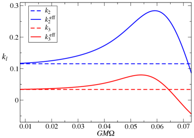
To characterize the effects of dynamical tides we introduce an effective tidal deformability that depends on the binary separation. Since the separation evolves under gravitational radiation reaction, is in fact a function of time. We define through
| (2) |
Note that in the adiabatic case . When we evaluate Eq. (2) for an inspiral using a dynamical quadrupole, the function can be understood as a varying tidal deformability. The deviation of from its constant value is an indication of the impact of dynamical tides.
In Sec. VI.5 we derive an approximate analytic expression for using a two timescale method. The result is shown in Fig. 1 and displays the enhancement of tidal effects due to dynamical tides close to merger or disruption. The quantities shown in this figure are the dimensionless Love numbers which are related to the deformability by
| (3) |
where is the radius of the neutron star and is the multipolar order ( for the quadrupole considered here, i.e., ). We work in units where , but we keep Newton’s constant . We use greek letters to denote spacetime indices that run over and latin letters running over the values for 3-dimensional spatial components.
I.2 Qualitative expectations for relativistic effects in dynamical tides
Relativistic corrections to the Newtonian tidal interactions discussed above are important to accurately describe tidal effects of binary neutron stars. Such corrections were computed in Ref. Vines and Flanagan (2013) within a post-Newtonian (PN) approximation to 1PN order and applicable for any kind of tides, and for the case of adiabatic tides the 2PN order was calculated in Ref. Bini et al. (2012). These studies showed that relativistic corrections enhance the tidal force acting on the body, which is a statement on the interaction term in Eq. (1). Moreover, by virtue of the equivalence principle, Eq. (1) provides an intuitive description of the relativistic case in a local freely falling coordinate system attached to the neutron star. Such local observer experiences a relativistic redshift relative to an observer at spatial infinity and also a frame dragging due to gravito-magnetic fields. This has interesting consequences for dynamic tides.
The physical consequence of the redshift effect can be understood as follows. All frequencies measured in the neutron-star’s frame are redshifted from the perspective of an observer measuring the gravitational waves at spatial infinity. This means that the f-mode frequency seen by the distant observer is redshifted with respect to the constant f-mode frequency in the rest frame of the neutron star. Conversely, from the perspective of the neutron star, the frequency of the driving tidal force is larger compared to that inferred by an asymptotic observer. This redshift effect is expected to enhance the dynamical tidal effects, since it shifts the resonance with the f-mode to a lower orbital frequency. The radiation reaction is therefore smaller at the resonance, such that the system spends more time close to the resonance and transfers more energy from the orbital motion to the tidal excitation.
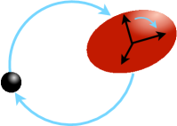
The consequence of the frame-dragging effect due to the gravito-magnetic field is somewhat opposite to the redshift effect. For a comparable mass system, the dominant angular momentum is the orbital one. Hence the neutron-star frame is dragged in the direction of the orbital motion as illustrated in Fig. 2. The orbital frequency in this dragged frame is therefore lower than for the distant observer. The frame dragging thus effectively shifts the f-mode to a higher frequency. This is analogous to the Zeeman effect for the splitting of atomic spectral lines in the presence of a magnetic field. Similarly, a bulge on the star rotates clockwise or counter-clockwise within the orbital plane, as a free oscillation. Invoking the equivalence principle, one infers that the bulge rotates with the constant f-mode frequency in both directions in the neutron-star frame. However, this frame is dragged as seen from a distant observer. This observer therefore sees different frequencies for the clockwise and counter-clockwise oscillations: the frequency of the bulge traveling in the direction of the orbit is shifted to larger values, while the frequency of the bulge traveling in the opposite direction is shifted to lower values. However, since the external tidal field always tracks the orbital motion, only the mode with the raised frequency is excited. A similar effect also occurs for neutron stars with spin Ho and Lai (1999), where, however, the direction of the dragging depends on the orientation of the spin. For a neutron star with a large spin that is anti-aligned with the orbital angular momentum, the resonance frequency is effectively lowered since in that case the spin drags the frame in the direction opposite to the tidal force.
The frame dragging is usually encoded in various spin interactions in a Hamiltonian formulation of the binary dynamics. This is true also for the frame dragging acting on the dynamical tides. Noether’s theorem applied to the rotational invariance of Eq. (1) shows that the tides contribute to the total angular momentum through a “tidal spin” given by the antisymmetric tensor . To obtain a complete tidal model it is essential to include a covariant generalization of this spin in place of the ordinary relativistic spin interaction terms in the Hamiltonian, whose importance was alluded to in Ref. Vines and Flanagan (2013), and which becomes obvious from Eq. (39) below.
I.3 Action for relativistic dynamic tides
Dynamical tides in general relativity have been studied in the case of a test-mass orbiting a neutron star Kojima (1987); Ruoff et al. (2001); Gualtieri et al. (2001); Pons et al. (2002) and for comparable masses in the PN limit focusing on r-modes Flanagan and Racine (2007). Resonances due to tidal interactions have also been seen in numerical-relativity simulations Gold et al. (2012) for binaries on eccentric orbits. An interesting dynamical response to a stationary tidal field was found recently for a slowly rotating neutron star Landry and Poisson (2015a). The authors of Refs. Maselli et al. (2012); Ferrari et al. (2012); Maselli et al. (2013) have developed a dynamical model for the tidal interaction of neutron stars by approximating them as triaxial ellipsoids with self-similar internal isodensity surfaces. This model takes into account the strong self-gravity of the neutron star, but does not include mode resonances in an explicit way. The effect on the gravitational-wave phase was found to be negligible Maselli et al. (2012). We come to a different conclusion here when dynamical tides are allowed to become resonant.
Let us write down a 4-dimensional covariant and minimally coupled form of the Lagrangian (1) as
| (4) |
with the full action principle of the matter being
| (5) |
where denotes a covariant parameter derivative, , , and the worldline of the particle is with being a generic worldline parameter. The signature of spacetime is . Note that in this notation , and the factors of are introduced such that the action is invariant under reparametrizations of the worldline parameter . For the gauge choice of adopted later on, takes on the physical meaning of the redshift factor. The 4-dimensional tidal field is the electric part of the Weyl tensor given by
| (6) |
which is reparametrization invariant and is a symmetric-tracefree spatial tensor in the rest frame, i.e., , , and . Similarly, the 4-dimensional quadrupole tensor is required to be a symmetric-tracefree spatial tensor in the rest-frame,
| (7) | |||
| (8) |
These are covariant constraints that reduce the quadrupole degrees of freedom to the correct physical ones. We explicitly relate to a SO(3) tensor in Sec. II.4 and highlight the connection of the equations of motion derived from the Lagrangian (4) to the dynamics of a generic extended body given by Dixon Dixon (1979) in Sec. II B. In Sec. III we compute the Lagrangian (4) within the PN approximation for the orbital dynamics. The PN results agree with the 1PN tidal Lagrangian derived in Ref. Vines and Flanagan (2013). However, the formalism developed in this paper features several advances beyond the standard PN approach such as (i) elucidating the role of the frame effects discussed above, which emerge from the constraint on the quadrupole in Eq. (7) and the covariant derivative in Eq. (4), (ii) exhibiting the redshift factors explicitly, and (iii) revealing a direct mapping between tidal effects and known PN results for spinning bodies, which we explain in Sec. III.
I.4 Body and orbital zones
The link between the action (5) describing a point particle with a dynamical quadrupole and the actual extended neutron star is established by introducing various zones in which different approximation schemes are valid. For instance, in the PN approximation, one introduces a body zone for each object where gravity can be strong, an orbital zone (or near zone) where the PN expansion in weak gravitational fields and slow motion can be applied, and a radiation zone where the emitted gravitational waves are weak and propagate with the speed of light.
The connection between the zones can be rigorously established using matched asymptotic expansions as summarized in Ref. Blanchet (2014). For binary black holes, an explicit construction of all zones has been developed in the context of initial data for numerical-relativity simulations Yunes et al. (2006); Yunes and Tichy (2006); Johnson-McDaniel et al. (2009); Gallouin et al. (2012); Mundim et al. (2014); Ireland et al. (2016). For neutron stars, the process of matching between body and orbital zones encodes the tidal interactions. An explicit construction of all the zones analogous to that for black holes is not yet available. However, this does not prevent us from obtaining a complete description of the orbital dynamics, since this requires only knowledge of the body’s multipole moments Flanagan (1998); Racine and Flanagan (2005). For stars with low compactness such as white dwarfs, the matching calculations can also be done by applying the PN approximation to the interior of the star, which was worked out to 1PN order by Damour, Soffel, and Xu Damour et al. (1991, 1992, 1993, 1994).
The matching of the body and orbital zones can be achieved by using a point-particle action as an intermediary, since it provides an immediate physical understanding, like the harmonic oscillator action in Eq. (4). Once the parameters defined by the action ( and ) are fixed through some matching, one can apply the point-particle model to a PN description of the orbital dynamics. One can think of the body zone being effectively shrunk to a point. Conversely, from the perspective of one of the bodies, the orbital scale can be expanded to spatial infinity. This leaves an isolated body in an external field, which is a rather simple setting in which the parameters in the action can be matched. For instance, the tidal parameters and can be obtained from linear perturbations of a spherically symmetric relativistic star. This approach properly incorporates the strong gravity inside relativistic stars, which is reflected in the numerical values for and . The quadrupolar Love number was first obtained from linear perturbations of a relativistic star in Ref. Hinderer (2008) and generalized to higher multipoles in Refs. Binnington and Poisson (2009); Damour and Nagar (2009). The latter study also raised important subtleties in defining the Love numbers through such a matching procedure Damour and Nagar (2009). Subsequently Ref. Kol and Smolkin (2012) showed how these subtleties are avoided in the case of nonrotating black holes. The rotating case is not settled, but progress has been made in the slow rotation approximation Poisson (2015); Landry and Poisson (2015b); Pani et al. (2015a, b). The matching of the f-mode frequency is likewise a delicate problem and the frequency entering the action (4) is distinct from the complex quasi-normal mode frequencies Kokkotas and Schmidt (1999); Nollert (1999). We discuss all these issues in detail in Sec. II.1.
I.5 Effective-one-body Hamiltonian
The impact of dynamical tides over adiabatic ones is expected to be noticeable only close to the f-mode resonance. This occurs in the strong-field regime of general relativity, where the PN approximation loses accuracy. Dynamical tides in general relativity therefore require a method which is applicable to the nonlinear orbital regime, such as numerical relativity. However, to enable the generation of a large bank of gravitational-wave templates for data analysis, a computationally much less expensive approach is needed. The EOB model is currently used for this purpose since it provides an accurate description of the entire gravitational-wave signal by combining analytical information from PN and black-hole perturbation theory into a single framework Buonanno and Damour (1999, 2000). The accuracy of the model has been further improved through a calibration to numerical relativity Taracchini et al. (2014); Nagar et al. (2016), thus creating a synergy of the most powerful tools to describe relativistic compact binaries.
The EOB model was extended to tidal effects in Refs. Damour and Nagar (2010); Baiotti et al. (2011); Bernuzzi et al. (2012); Bini et al. (2012); Bini and Damour (2014); Bernuzzi et al. (2015), but restricted to adiabatic tides. The purpose of the present paper is to improve the description of matter effects by considering dynamical tidal effects in the EOB Hamiltonian. In contrast to Ref. Bini et al. (2012), our construction implements the test-particle results without introducing poles in the Hamiltonian (see Secs. V.2 and VI.3). This is important for neutron-star–black-hole systems, where for certain mass ratios the poles might be reached during the final stages of the binary evolution. The main result for the EOB Hamiltonian is given by Eqs. (83), (VI.1)–(120), (130a)–(130c), and (137) for circular orbits. This result is accurate to 1PN order and further contains partial information at 2PN order in Eq. (130a) determined by matching to the adiabatic limit from Ref. Damour and Nagar (2010). We also study different, structurally less motivated, implementations of dynamical tides in the EOB Hamiltonian to verify that our conclusions are not an artifact of the specific implementation. Our results are the foundation of EOB waveforms with fully dynamical tides that have been compared against numerical-relativity simulations in Refs. Hinderer et al. (2016); Taracchini et al. (2016). The tidal EOB Hamiltonian can equivalently be obtained from the generic 1PN tidal Lagragian derived in Ref. Vines and Flanagan (2013). The benefit of starting from a relativistic action is that it leads to immediate insights into the structure of the terms, thus providing physical intuition as well as useful guidance for devising an EOB resummation of tidal effects.
The plan of this paper is the following. We first discuss the general relativistic point-particle action encoding dynamical tides in Sec. II. To express the terms in this action explicitly, we specialize to the PN and test-particle approximations in Sec. III. This is the basis for the EOB Hamiltonian derived in Sec. VI, following the construction principles outlined in Sec. IV and making use of the gauge freedom from Sec. V. Finally, the results are discussed in Sec. VII where we compare waveforms including dynamical tides with waveforms using only adiabatic tides. We find that dynamical tides are an important physical effect for certain realistic nuclear equations of state and mass ratios.
II Theory of relativistic dynamical tides
In this section we discuss in detail the effective point-particle action for dynamical tidal effects in general relativity. We first review Newtonian dynamic tides to motivate the covariant form of the relativistic action (4) which we determine within an effective-field-theory approach. Next, we consider the equations of motion and Legendre transformations that bring the action into a convenient form. Lastly, we impose the constraints by separating the time and spatial components of the tidal variables to derive an action that involves only the physical tidal degrees of freedom.
II.1 The effective action
Below we discuss the reasoning that led us to posit the particular form of the Lagrangian (4) for a relativistic action that describes quadrupolar mode oscillations of a deformable body. We start by reviewing the Newtonian description of stellar oscillations to make the relation between the mode amplitudes and the quadrupole degrees of freedom explicit. Subsequently, we use the effective-field-theory approach for compact binaries developed by Goldberger and Rothstein Goldberger and Rothstein (2006a); Goldberger (2007) to obtain a covariant version of the Newtonian action that leads to Eq. (4). Previous work on this topic already derived the quadrupolar interaction terms Goldberger and Rothstein (2006b); Goldberger and Ross (2010) and considered a dynamical quadrupole in the context of absorption from the black-hole horizon Goldberger and Rothstein (2006b). Other work Bini et al. (2012) obtained an effective action in the limit of an expansion around the adiabatic case. Here, we go beyond these studies by deriving a general effective action for a fully dynamical quadrupole that describes mode oscillations of a deformable body. We further discuss subtleties related to the identification of the coupling constants and , survey additional terms that could in principle contribute to the action, and argue that in the case of interest here these terms are negligibly small.
Generic tidal perturbations of a Newtonian star can be decomposed into its normal modes of oscillation Chandrasekhar (1964), and are an extensively studied topic. An action principle for the mode amplitudes was formulated by Alexander Alexander (1987), and also derived from Lagrangians for an ideal fluid polytrope Gingold and Monaghan (1980), for homentropic stars Rathore et al. (2003), and from an effective-field-theory approach Chakrabarti et al. (2013a). These action principles rely on treating the amplitude of each mode as a harmonic oscillator. Since the unperturbed star is rotationally symmetric, the modes fall into irreducible representations of SO(3). This implies that the quadrupolar mode variables, which are usually decomposed into a spherical-harmonic basis with and , can equivalently be described by rank-two symmetric-tracefree tensors, denoted here by , with . The Lagrangian for the quadrupolar f-mode amplitudes therefore has the form
| (9) |
where the constants and are the angular frequency and coupling constant, also known as the “overlap integral” Press and Teukolsky (1977), of the mode, is the quadrupolar tidal field, and the dots denote possible nonlinear interaction terms. The Lagrangian in Eq. (9) differs from Eq. (1) only by a choice of normalization, where
| (10) |
It is straightforward to extended this result to several quadrupolar modes by adding copies of Eq. (9) for each mode. However, if the normal-mode expansion fails to represent the complete solution for the perturbed star, copies of Eq. (9) for each mode will be insufficient to represent the entire quadrupolar response of the star and additional terms of the form must be included in the Lagrangian (9) to compensate for the residual discrepancy. For Newtonian perfect fluid stars, the normal modes are complete Cox (1980) and hence no such additional terms are required. In this case, the constants and (or ) entering the Lagrangian are easily identified with quantities computed from linear perturbations of a fluid star Cox (1980); Love (1909). The dominant modes for tidal interactions are the f-modes, whose tidal coupling constants are several orders of magnitude larger than those of other quadrupolar modes Shibata (1994); Kokkotas and Schäfer (1995), hence we neglect those other modes here.
To obtain a relativistic generalization of the Newtonian Lagrangian (1) we employ the effective-field-theory approach to the gravitational interaction of compact objects Goldberger and Rothstein (2006a). In this approach, the interaction terms in the action are determined by writing down all possible operators consistent with the symmetries (general covariance, parity, and time reversal), and redefining variables to eliminate couplings that involve accelerations Damour and Schäfer (1991). For the linear, electric-type, quadrupolar interactions these considerations lead to a single interaction term derived in Ref. Goldberger and Rothstein (2006b) and given by , with the relativistic tidal field defined in terms of the spacetime curvature in Eq. (6). This generalizes the Newtonian coupling and the Newtonian definition of . The remaining steps in mapping from the Newtonian to the relativistic action consist in replacing time derivatives with covariant derivatives along the worldline, and inserting factors of to ensure invariance of the action under reparametrizations of the parameter . In general, as discussed above in the Newtonian case, tidal couplings of the form may need to be added to the Lagrangian (4). Such terms would account for the incompleteness of modes which is known to occur in general relativity, as well as for other quadrupolar modes besides the f-modes. However, as in the Newtonian case, the coupling coefficients of these additions are estimated to be small Chakrabarti et al. (2013b) and we therefore neglect these additional terms here.
As mentioned in Sec. I.4, the relativistic effective action (5) discussed above describes the binary only on an orbital scale, where the coefficients and remain undetermined and must be linked to quantities describing a perturbed relativistic fluid star through a matching procedure. In contrast to the Newtonian case, the relativistic nonlinearities introduce subtleties into this identification and can lead to counter-intuitive results. For instance, the Love number of black holes vanishes Kol and Smolkin (2012), which is impossible to reproduce through a superposition of damped mode amplitudes as would be done when extrapolating Newtonian results. While neutron stars are less compact than black holes, they nevertheless enclose strong gravitational fields and might inherit some non-intuitive features. A rigorous definition of their tidal deformability coefficients requires performing an analytic continuation in the dimensionality of spacetime as done for the case of black holes in Ref. Kol and Smolkin (2012) or, as a more practical but less rigorous alternative, using the prescription for neutron stars developed in Ref. Chakrabarti et al. (2013b). Likewise, the real mode frequency parameter in the Lagrangian follows from a matching of the orbital and body zones as discussed in detail in Ref. Chakrabarti et al. (2013b). The boundary conditions of this matching are different from those used to define the complex quasi-normal mode frequencies Kokkotas and Schmidt (1999); Nollert (1999), yet the numerical value of determined in this way turns out to be very close to the value of the real part of the quasi-normal mode frequency Chakrabarti et al. (2013b).
Having discussed the construction of the relativistic action for fully dynamical quadrupoles, it is also useful to consider the limiting case far from a resonance where the quadrupole is nearly adiabatic, to establish a connection with previous work in Refs. Bini et al. (2012); Chakrabarti et al. (2013a). The effective-field-theory paradigm states that all degrees of freedom with frequencies above the orbital frequency should be integrated out of the action. Thus, when restricting the description to tidal driving frequencies that cannot excite the f-mode, the tidal Lagrangian (4) is approximated by a quasi-adiabatic Lagrangian Bini et al. (2012); Chakrabarti et al. (2013a)
| (11) |
with the dots denoting similar terms with higher-order derivatives of . The first term in Eq. (11) corresponds to the adiabatic limit and the second term is the first correction due to dynamical tides, with the coefficient determined in terms of (, ) by the Taylor expansion
| (12) |
i.e., , and similarly for the omitted higher-order terms. Close to the resonance, such an expansion of the Lagrangian around the adiabatic limit in Eq. (11) breaks down since the resonance corresponds to a pole in the response. Cases for which the inspiral terminates well before the resonance is reached could be adequately described by retaining a finite number of terms in Eq. (11). This would avoid the introduction of additional dynamical variables for the quadrupole, which is computationally expensive. However, in Sec. VI.5 we introduce a significantly more useful method for reducing the computational cost while still capturing the nonlinear features of the resonance.
II.2 Equations of motion
To study the dynamics described by the action (4) we first obtain the equations of motion using a manifestly covariant variation as described in detail in Ref. Steinhoff (2015). Ignoring the constraint in Eq. (7) for the sake of clarity,222The constraint (7) is preserved if the secondary constraint holds. The method of Lagrange multipliers legitimizes our procedure, since it fixes the multipliers of these constraints to zero, up to terms of negligible order in the curvature. this leads to
| (13) | |||
| (14) |
Here, we have introduced a “tidal spin” tensor associated with the angular momentum of the dynamical quadrupole and a rank-4 quadrupole moment given by
| (15) | ||||
| (16) |
The generalized momenta in Eqs. (13) and (14) are defined by
| (17) | ||||
| (18) |
where the partial derivatives of the Lagrangian are calculated assuming the functional dependence
| (19) |
Our convention for the Riemann tensor is
| (20) |
where is the Christoffel symbol.
Since we are considering here an irrotational matter configuration, the presence of spin terms in the equations of motion requires further explanation. The interpretation is that the tidal bulge carries an angular momentum given by Eq. (15) since the bulge points towards the companion and thus travels around the neutron star’s surface during an orbit. However, this angular motion of the bulge is due to fluid elements undergoing only a radial motion; hence the neutron star itself remains irrotational. Yet, it has a net spin given by the sum of the spin due to the rotation of the fluid, which vanishes in the case considered here, and the tidal angular momentum . The dynamics of the tidal spin are analogous to those of an intrinsic spin, obeying the generic form of the equations of motion for the spin-dipole found by Dixon Dixon (1979),
| (21) |
which can be verified using the quadrupolar equations of motion (14) and (18). Dixon’s general multipolar approximation scheme fully determines the equations of motion only for the linear momentum and spin-dipole of the body. The equations of motion for all higher multipoles are not restricted by the conservation of energy and momentum, and depend on the internal structure of the body. Therefore, information about the internal dynamics of the higher multipoles must be supplemented to Eqs. (13) and (21). An example of such supplemental information to complete the set of equations of motion is the oscillator dynamics describing f-modes in Eqs. (14) and (18). This example also illustrates that the tensors describing the spin and higher multipole moments in Dixon’s equations of motion, in this case the quantities in Eqs. (15) and (16), are in general merely mathematical structures that represent combinations of more fundamental degrees of freedom.
Having developed insights into the covariant dynamics discussed above, we next turn to the idea of using the action (4) to derive a fully constrained Hamiltonian that can be mapped to an EOB model. This requires transformations of Eq. (4) that involve the following steps. First, we replace all velocities in favor of the conjugate momenta, include the mass-shell constraint in the transformed action, and perform a decomposition of all the quantities into time and space directions. Next, we obtain explicit expressions for the various terms in the resulting Lagrangian within the PN approximation, as well as in the test-particle limit, and construct the corresponding Hamiltonian. Finally, we investigate several possibilities for mapping this information onto the EOB model. In the subsequent sections we present a detailed discussion of each step in this procedure.
II.3 Legendre transformations
Following Refs. Steinhoff (2011, 2015), we apply a Legendre transformation and rewrite the action in Eq. (4) in the following equivalent form
| (22) |
where
| (23) |
The action (22) has the advantage that the complicated covariant derivative of appears only linearly and only in a simple kinematic term, which is convenient for explicit calculations.
A further Legendre transformation can be performed to replace by . This is interesting since it manifestly brings the action into first-order form in all variables, which is necessary for a Hamiltonian formulation. From Eq. (17) we have
| (24) |
Using the normalization of the four-velocity leads to the mass-shell constraint
| (25) |
with
| (26) | ||||
| (27) |
where we neglect terms of higher order in curvature and tidal variables. [Note that this result is analogous to Eq. (85) in Ref. Steinhoff (2015), but with a factor of 2 typo in the interaction term corrected here.]
The mass-shell constraint (25) is in fact a special case of a general first-class constraint associated with a gauge freedom. Here, the gauge symmetry is the reparametrization-invariance of the worldline parameter , with its associated gauge freedom represented by the length of . This leads to the feature that the relation (24) depends only on the normalized four-vector and is noninvertible. Following the usual procedure in constrained dynamics Dirac (1950, 1964), the constraint (25) must be added to the action using a Lagrange multiplier
| (28) |
with the canonical Hamiltonian being zero. In this form of the action, the function is undetermined and represents the gauge freedom of the original action (22). Note also that in (28) the mass-shell constraint takes the place of the Hamiltonian and all interactions enter as deformations of the mass shell. This is an important point of view for constructing the test-particle–limit (and then EOB) Hamiltonian, as we shall see in Secs. III.3 and IV.
II.4 Imposing the tidal constraints
In this section we impose the constraints on the tidal variables from the action in Eq. (22) through an explicit split into spatial and time components.
We perform the decomposition of and to single out their spatial SO(3)-irreducible parts. As discussed below Eqs. (7) and (8), in the body’s rest frame the quadrupole is a symmetric-tracefree spatial tensor. Its conjugate momentum shares the same properties and satisfies the same constraints to linear order in the tidal variables, as can be shown by taking a time derivative of Eq. (7) and using the definition (18). Therefore, to single out the independent spatial components of and we perform a Lorentz boost to the rest frame. For this purpose, we project the tidal variables onto a tetrad , defined such that , where is the Minkowski metric. The quadrupole can thus be expressed in terms of its components on the local Lorentz frame as . The next step is to apply a Lorentz boost to transform and to the rest frame which we denote by a tilde,
| (29) |
A particularly simple boost to the rest frame is given by
| (30) |
which is sometimes referred to as a standard boost. This boost has the properties , , and . This implies that the constraints and become in the rest frame, where the round brackets around an index denote the local frame. The SO(3)-irreducible components of and are therefore the spatial symmetric-tracefree tensors and . The transformation to the tetrad frame is
| (31) | ||||
| (32) |
To simplify the notation, we henceforth drop the tilde and the round brackets for the spatial indices of certain tensors. Specifically, we define
| (33) | |||
| (34) |
and we also omit the round brackets on indices of since it is used in the local frame only.
We next consider the split of the action in Eq. (22) into space and time starting with the tidal kinematic term
| (35) |
Interestingly, the combination of boosts in the last term also appears in the computation of spin effects Levi and Steinhoff (2015). Here only the last term of Eq. (3.18) in Ref. Levi and Steinhoff (2015) gives a nonvanishing contribution leading to
| (36) |
It is important to note that can only be inserted in Eq. (36) after expanding the covariant derivative using that
| (37) |
Here, the Ricci rotation coefficients are defined to be , the Christoffel symbols are , and in this section a dot denotes a derivative with respect to . Thus, the decomposition of the tidal kinematic terms is explicitly given by
| (38) |
with
| (39) |
Here FD stands for frame dragging, whose physical origin was explained in the Introduction. These interaction terms are identical to those in the effective action of ordinary spin effects [as given in Eq. (5.27) of Ref. Levi and Steinhoff (2015)].
We continue the split into space and time components of the action (22) with the decomposition of the tidal interaction term,
| (40) |
where we use the notation . This term likewise has a corresponding analog in the ordinary spin calculations given by the spin-induced quadrupole, which is discussed below. Finally, the oscillator part of the Lagrangian is
| (41) |
Note that the dependence on the metric enters only through the overall factor , which is the same for the point-mass part, i.e., . Thus, one can view the pure oscillator part as a shift of the mass , see Appendix C.
III Post-Newtonian and test-particle approximations
In this section we explicitly derive all the terms entering the action (42) to 1PN order and obtain the Hamiltonian. The PN approximation requires integrating out the potential or near-zone “modes” of the gravitational field Goldberger and Rothstein (2006a); Goldberger (2007) and usually involves lengthy Feynman integral calculations. Here, however, we can bypass these computations by exploiting connections to the point-mass and spin sectors and simply apply certain replacements to PN results from Ref. Levi and Steinhoff (2015). Previous results for the action using different approaches were obtained at 1PN order Vines and Flanagan (2013) and, in the adiabatic limit at 2PN Bini et al. (2012), see Sec. I.2. In addition to the PN limit of the action, we also consider the test-particle limit, which provides information about the strong-field behavior.
III.1 Potential at 1PN order
The PN approximation is a weak-field and slow-motion approximation with orders counted as powers of , where is the velocity of the object and is the orbital separation. In this framework, tidal effects are suppressed by a multipolar approximation parameter, which, for the even-parity -polar tidal interaction, is given by
| (43) |
where is the object’s radius, and for the leading-order tidal effects considered here. For black holes, , which means that the multipolar suppression meshes with the PN power-counting scheme and the conclusion from Eq. (43) is that tidal effects start only at 5PN order. However, for neutron stars so that the multipolar scaling fails to mesh with the PN counting. Therefore, tidal effects are considered to start at Newtonian order. In this section, we work out the next-to-leading or first PN (1PN) corrections to tidal effects and compare to the findings in Ref. Vines and Flanagan (2013).
We introduce the following notation. The tidally deformed body is labeled as number 1 and its point-mass companion as number 2, where the labels are also used for the corresponding masses and orbital variables. The index denotes a generic particle label. We continue to give explicit results only for the case of one tidally deformed body, noting that all the expressions can readily be extended to the case of two deformed bodies by adding a copy of all the tidal terms with the particle labels interchanged. For the worldline parameter, we choose the gauge , where is the coordinate time that coincides with the time measured by an asymptotic observer.
For the subsequent PN analysis it is convenient to express the action (42) in terms of the PN potential as
| (44) |
where is the point-mass Lagrangian in the PN approximation. Here, the subscript “pm” denotes a point-particle having only a mass monopole. The PN approximated tidal potential is decomposed as
| (45) |
where each part of Eq. (45) is discussed and derived in detail below.
The contribution arising from the oscillator (41) is obtained as follows. As already noted, the dependence on the gravitational field enters in this term only through the overall factor of , which is the same in the point-mass part. We can therefore obtain the PN potential associated with Eq. (41) by a linear shift of the mass in the non-tidal part of the Lagrangian which leads to
| (46) |
where we use
| (47) |
To 1PN order this is explicitly
| (48) |
where , . It is crucial here that is treated as an independent variable, otherwise the dependence of in Eq. (41) on the gravitational field would be more complicated. The physical interpretation of the quantity is that it is the redshift between the proper time of the worldline and the asymptotic observer with time . The fact that the redshift can be obtained from the formula (47) was first realized in the context of the first law of mechanics for binary black holes Blanchet et al. (2013). This can be understood by observing that arises from the procedure of integrating out the potential modes of the point-mass Lagrangian . This procedure does not affect the physical meaning of the partial derivative in Eq. (47), hence we have
| (49) |
In the last step we used the definition of the proper time and the gauge .
Consequently, the PN corrections to the pure oscillator part have a simple physical interpretation. When the oscillator is described in terms of the proper time , it is an ordinary Newtonian oscillator, in accordance with the expectations from the equivalence principle. The PN corrections in are due to the redshift to the asymptotic observer with time , which is used to describe the dynamics in PN theory and which is measured by the gravitational-wave detectors. This leads to an effective redshift of the resonance frequency away from its value measured in the frame of body 1.
The contribution from the interaction terms in Eq. (45) is associated with the Lagrangian in Eq. (40). This term is analogous to the spin-induced quadrupole coupling described in Refs. Poisson (1998); Porto and Rothstein (2008); Levi and Steinhoff (2015)
| (50) |
where the spin vector is defined by
| (51) |
and is the completely antisymmetric volume form. The spin potentials are expressed in terms of the canonical spin denoted by a hat. This spin is given by the spatial components of the spin tensor which satisfies the Newton-Wigner condition . Using this condition and the definitions given above, one can show that . Therefore the spins in Eq. (50) are those appearing in the final PN potential. The potential associated with Eq. (40) can therefore be obtained by substituting the tidal quadrupole in place of the spin quadrupole using the identification
| (52) |
This further implies the substitution since is tracefree. Using these replacements in the 1PN expressions for the spin-induced quadrupole interaction potential given in Eqs. (6.10) and (6.40) of Ref. Levi and Steinhoff (2015) or equivalently in Ref. Hergt et al. (2010) leads to
| (53) | ||||
where , . This result can readily be extended to 2PN order by applying the spin to tidal-quadrupole mapping (52) to the expressions in Ref. Levi and Steinhoff (2016a).
The last term in Eq. (45) describes the interaction of the orbital and tidal angular momentum given in Eq. (39), which, as discussed above, is identical to the ordinary spin interaction terms in PN theory. We can therefore obtain the corresponding potential by replacing the spin by in the PN spin potentials that are already available. Note that this replacement only works because is independent of the field and instead depends only on the two independent tensors and . Applying the spin to tidal-spin transformation to the leading-order spin-orbit potential from Eq. (6.3) in Ref. Levi and Steinhoff (2015) leads to
| (54) |
where . Previous alternative derivations of the result (54) can be found in Refs. Tulczyjew (1959); Damour (1982); Damour and Schäfer (1988).
This potential is at 1PN order in the tidal case, but in the literature it is usually counted as a 1.5PN spin effect. This happens because the counting of the ordinary spin effects usually assumes a rapidly rotating (extremal) black hole whose spin is considered to be a PN contribution, while the tidal spin is fixed by the Newtonian counting of the quadrupole through Eq. (34). The potential could be extended to 3PN order (3.5PN in the ordinary counting) using the results of Refs. Hartung and Steinhoff (2011); Levi and Steinhoff (2016b). These interaction terms have the physical interpretation that they describe the frame-dragging effect due to a gravito-magnetic field, as explained in Sec. I.2 above. The intimate connection between spin and frame dragging is evident in the case of a small test spin, which stays constant in a local inertial frame but can change direction as seen by a distant observer. In general, the particle’s worldline deviates from geodesic motion, e.g., due to tidal forces. Thus, the frame associated with the worldline is not inertial, but follows a Fermi-Walker transport. This is encoded in the acceleration-dependent term in Eq. (54). Since we consider the case of an irrotational star, we refer to as frame dragging rather than a spin effect.
The final result for the 1PN tidal Lagrangian (44) is then obtained from Eq. (45) together with Eqs. (46), (53), and (54). A similar result was derived from the PN equations of motion in Ref. Vines and Flanagan (2013). Taking into account the different conventions, we find that the difference between the two expressions is a total time derivative given by
| (55) |
where is the Lagrangian from Ref. Vines and Flanagan (2013), , and we specialize to the adiabatic limit in . We can further obtain an equation of motion for the tidal angular momentum, which at Newtonian order reads
| (56) |
in agreement with the tidal torque in Eq. (1.7) in Ref. Vines and Flanagan (2013) and our covariant Eq. (21). While the method based on the PN equations of motion Vines and Flanagan (2013) and the effective action approach developed here lead to identical results, the advantage of using the effective action is that it makes the underlying structure of the terms (such as the redshift factors) explicit, and clarifies the relevance of the tidal spin. These insights further facilitate the extension of the results to higher PN orders and the identification of several tidal contributions for which existing results about point-mass and spin potentials can be used.
III.2 Hamiltonian at 1PN order
Implementing dynamical tidal effects in the EOB formalism first requires deriving the Hamiltonian associated with the Lagrangian (44). This can be accomplished by employing a reduction of order to remove higher-order time derivatives in the potential using the equations of motion Damour and Schäfer (1991), followed by a Legendre transformation of the velocities. We apply this procedure to the 1PN tidal Lagrangian in Eq. (44) using the Newtonian equations of motion . Similarly, to perform the Legendre transformation it is sufficient to use the Newtonian relations , where are the canonical momenta conjugate to . Since the Hamiltonian can be directly obtained from these substitutions, we refrain from showing this intermediate result here. Next, we transform to the center of mass frame where . This results in the following 1PN accurate Hamiltonians
| (57) | ||||
| (58) | ||||
| (59) |
| (60) |
where and .
To derive the Poisson bracket relations and demonstrate that and and and are canonically conjugate pairs, it is useful to consider the action expressed in the form
| (61) |
where is the point-mass Hamiltonian in the PN approximation and the tidal Hamiltonian is
| (62) |
The redshift can be obtained from the Hamiltonian through
| (63) |
Note that the reduction of order in the Lagrangian implicitly also entails a redefinition of the variables as discussed in Ref. Damour and Schäfer (1991). Therefore, the canonical momenta do in general not agree with the spatial components of .
The equations of motion obtained from varying the action (61) have the structure of Hamilton’s equations and are equivalent to the Poisson brackets
| (64) | ||||
| (65) |
with all others being zero. The quadrupolar symmetric-tracefree projection operator is given by
| (66) |
It follows that the tidal angular momentum obeys a canonical SO(3) angular-momentum algebra,
| (67) |
However, the tidal angular momentum has nonvanishing brackets with other variables,
| (68) | ||||
| (69) |
This algebra implies that is the generator of infinitesimal rotations for the tidal variables. The interaction terms involving therefore effectively rotate or drag the frame of the tidal variables. The Poisson brackets (68) agree with the bracket algebra for internal degrees of freedom of a spinning particle in general relativity constructed in Ref. Tauber (1988).
III.3 Test-particle Hamiltonian
The PN approximation discussed above is only valid for slow motion and weak gravitational fields, but generic mass ratios. By contrast, the small-mass-ratio approximation is valid for generic velocity and field strength, but is limited to perturbations of the test-particle limit. The EOB model provides a unified framework to incorporate both the PN and test-particle results in the respective limits, bridging between them. As a first step in building a dynamical tidal EOB Hamiltonian, in this section, we derive the dynamical tidal Hamiltonian in the test-particle limit following the method in Ref. Vines et al. (2016). The adiabatic limit of the tidal Hamiltonian in the test-particle case for circular orbits was computed in Ref. Bini et al. (2012). Furthermore, the frame-dragging contributions can be found in Refs. Barausse et al. (2009); Vines et al. (2016), where the spin should be mapped to the tidal spin. In order to focus on the new terms in this section, we therefore omit these known frame-dragging contributions entering via Eq. (38).
We start from the action principle given in Eq. (28). Neglecting frame effects in Eq. (38), one can pass to the SO(3)-irreducible tidal variables by simply replacing 4-indices by local 3-indices. The action principle then becomes
| (70) |
where as before the dynamical mass is and the tidal Hamiltonian is
| (71) |
We replace the mass by here for later convenience. All interactions are encoded in a deformation of the mass-shell constraint,
| (72) |
which follows from the variation of .
We next reduce the orbital variables to their physical components, choosing the coordinate time as the worldline parameter , or , as we did in the PN case. Solving the mass-shell constraint (72) for , we obtain the action in the form
| (73) |
where is the Hamiltonian in the test-particle limit (TPL). To obtain explicit expressions for the potentials in the Hamiltonian we insert the metric in Schwarzschild coordinates into the mass-shell constraint, since similar coordinates are used in the EOB model. The solution of the mass-shell constraint then leads to
| (74) |
where . We see from Eq. (74) that the tidal Hamiltonian enters as a shift of the test-mass , which is expected based on the form of the mass-shell constraint (72). The subscript on the linear momentum vector denotes that components are taken in the local tetrad frame ,
| (75) |
and . Here the tetrad was chosen as the symmetric matrix square-root of the metric. Since scales with the fourth power in the mass ratio, we can expand in as
| (76) |
where the redshift is
| (77) |
To derive the expression for the tidal Hamiltonian we decompose it as
| (78) | ||||
| (79) | ||||
| (80) | ||||
where we have obtained from the mapping in Eq. (52) and Ref. Vines et al. (2016) in the limit of vanishing Kerr parameter. In these expressions, one can interchangeably use or within our approximation and the quantity is
| (81) |
In Eq. (80) we have also introduced a vector so as to express the Hamiltonian in a manifestly rotation-invariant form. This facilitates the use of Cartesian-like frames that are used in PN computations whereas the frame used above is adapted to spherical coordinates and is therefore noninertial in the Newtonian limit. Hence the frame effects involving , which we ignored in this section, cover not only relativistic frame-dragging effects, but also Newtonian frame effects (e.g., the Coriolis force). This becomes more apparent in an explicit calculation below.
Although the test-particle Hamiltonian (80) is already rather simple, we can make a further useful approximation, namely that the motion is along circular orbits so that . In this limit the tidal interaction Hamiltonian reduces to
| (82) |
where . An interesting feature of this circular-orbit version of is that no other terms beyond the 1PN approximation appear.
IV Construction of the effective-one-body Hamiltonian
In this section we map the above analytical results for relativistic dynamical tides into the EOB Hamiltonian describing the conservative dynamics of the binary. The full EOB waveform model, including dissipative effects, is discussed in Ref. Taracchini et al. (2016). The implementation of generic quadrupoles discussed here immediately applies also to spin-induced quadrupoles via Eq. (52), which can be useful for improvements of EOB models for spinning binaries.
IV.1 Structure of the Hamiltonian
In the EOB approach, incorporating the properties of the bodies other than the masses is non-trivial. For instance, in the case of spinning black holes, different proposals exist Taracchini et al. (2014); Nagar et al. (2016). The task of incorporating the effects of dynamical quadrupoles is qualitatively very different from including black-hole spins, since they further involve the internal dynamics of the bodies. In this section, we therefore elaborate on the basic principles behind the construction of the EOB Hamiltonian to motivate our prescription for incorporating dynamical tidal effects in the EOB model.
The EOB Hamiltonian is based upon an effective Hamiltonian describing the motion of an effective particle in an effective metric Buonanno and Damour (1999). In the test-particle limit, the effective metric can be chosen as the Schwarzschild or Kerr metric so that the test-particle limit is incorporated in a natural manner. For generic mass ratios, the mapping between the Hamiltonians is
| (83) |
where is the reduced mass and . While alternatives to this map were considered in the literature Buonanno and Damour (1999); Damour et al. (2000), no compelling reason was found to modify it away from this simple form, except for the one found in Appendix C here. The action corresponding to the EOB Hamiltonian is
| (84) |
To construct the effective Hamiltonian it is useful to recall that in the Newtonian limit, the motion of a binary can be mapped to the motion of a reduced mass in a central potential of mass . Hence it is natural to start out the EOB construction with a particle of mass moving in a (deformed) effective metric of mass . The effective Hamiltonian, being a test-particle Hamiltonian, is then given by (see Sec. III.3), where follows as the solution of the mass-shell constraint
| (85) |
Here incorporates possible effective interactions which lead to a non-geodesic (NG) motion, analogous to the tidal interactions in Sec. III.3. For the time being, we consider to be a generic symbol, but assume that a possible dependence on can be treated perturbatively as in Eq. (81) when solving the mass-shell constraint.333Note that is related to the potential introduced in Ref. Damour et al. (2000) The effective Hamiltonian for a generic effective metric is then given by
| (86) |
where
| (87) |
and is the inverse of the spatial effective metric ,
| (88) |
The effective metric and are fixed by requiring that agree with the PN and test-particle Hamiltonians in the respective approximations.
IV.2 Matching to the test-particle limit
Since the foundation for the structure of the effective Hamiltonian is the test-particle limit, we first discuss the inclusion of dynamical tides in the test-particle EOB Hamiltonian. In the test-particle limit the EOB and effective Hamiltonians are related by
| (89) |
where the factors of masses are due to the different rest-mass energies of the two Hamiltonians. The test-point-mass limit is then reproduced by taking the effective metric to be the Schwarzschild metric.
To incorporate the case of a test-particle with dynamical tidal degrees of freedom we consider the mass-shell constraint in Eq. (72) which is explicitly given by
| (90) |
where we have linearized in the tidal terms. Comparing this expression to the constraint given in Eq. (85) to identify the tidal contributions to the effective metric and the non-geodesic term does not lead to a unique identification. To fix this freedom, we choose the prescription that all terms that are quadratic in in Eq. (90) result from a contraction with the effective metric. This implies that contributes to the effective metric, which follows from the interaction term in Eq. (71) together with the definition (6) and using that within our approximations and are interchangeable in this term. The effective metric is then given by
| (91) |
Furthermore, note that the pure oscillator part is independent of and hence must be included in the non-geodesic term leading to the result . It is noteworthy that the effective metric is deformed away from the Schwarzschild metric even in the test-particle limit here, in contrast to non-tidal EOB models where the deformation starts at linear order in the mass ratio.
Using the above conventions to construct the effective Hamiltonian in Eq. (86) leads to the following prescription. All the terms in the mass-shell constraint (90) that are quadratic in , as seen explicitly by substituting the expression (80) for , are resummed in , while all terms linear in and in contribute to the potential , all terms quadratic in contribute to , and all remaining terms are included in . The importance of having access to additional information from the mass-shell constraint to determine these assignments is highlighted in Appendix C.
V Gauge freedom with dynamical tidal effects
Having derived the general structure of tidal contributions to the EOB Hamiltonian based on the test-particle limit, we next discuss several manipulations that are necessary to map the PN results into tidal corrections to the EOB functions. In this section we focus on gauge transformations. We first derive the 1PN accurate general canonical transformation from harmonic to EOB coordinates including the tidal terms. We subsequently apply the method of canonical transformations to obtain a rigorous derivation of the circular-orbit limit. Lastly, we present a convenient choice of frame for the degrees of freedom of the dynamical quadrupole.
V.1 Tidal terms in the gauge transformations
To express the PN Hamiltonian in the form required by the EOB Hamiltonian we apply a canonical transformation with generator to obtain
| (92) |
This transformation can be evaluated by making a general ansatz for and for the PN expansion of the EOB potentials that are invariant under rotations and translations, each involving undetermined coefficients, and solving (92) at each PN order. The solutions for the coefficients are in general not unique, which allows for further simplifications or convenient choices. The resulting canonical transformation can be viewed as a change of gauge on phase space with the choices for the free coefficients defining the gauge(s) of the EOB model.
To proceed, we split the canonical transformation into point-mass and tidal parts,
| (93) |
The point-mass part to 1PN order reads Buonanno and Damour (1999)
| (94) | ||||
This generator and the point-mass potentials are uniquely fixed by the requirement that the effective Hamiltonian is identical to the test-particle Hamiltonian, that is, no corrections in the mass ratio are necessary. At 2PN order, however, this requirement can no longer be satisfied. [Yet, the -dependence in Eq. (VI.1) below can in fact remain unaltered at higher PN orders. This invariance can be interpreted as a gauge-invariant meaning of the radial coordinate as the “centrifugal” radius Damour and Nagar (2014).]
For the tidal part of the canonical transformation, we choose an ansatz such that the transformation only generates terms having the same structures as already present in the 1PN Hamiltonian (III.2). This excludes generators involving and requires the generator to be linear in and at most quadratic in the tidal variables. This leads to the general form
| (95) |
where the coefficients parametrize the freedom in the PN coordinates. Here, the term involving that is quadratic in is associated with frame effects, which are discussed in detail in Sec. V.3 below. To avoid terms of the form , which do not appear in the Hamiltonian up to 1PN order, we set . The generator is an additional contribution that is necessary for imposing the circular-orbit limit at the level of the Hamiltonian. It will be discussed in the next section and is given by
| (96) |
Note that this generator should only be used for specializing to circular orbits since it would otherwise produce unusual terms due to the factor of in the denominator.
Another possible term in the generator is the combination
| (97) |
The prefactor here is the Newtonian Hamiltonian, which approximately commutes with in Eq. (92) and therefore does not produce structurally new terms, so that it is formally allowed. However, this transformation produces terms proportional to the kinetic and potential energies of the oscillator in Eq. (57), but with the opposite relative sign. Since the structure in Eq. (57) persists to all PN orders, we can exclude terms like Eq. (97) in the generator of the canonical transformation. However, for alternative choices of the EOB mapping not considered here, where the kinetic and potential oscillator energies are included in different potentials of the EOB Hamiltonian, the generator in Eq. (97) carries a nonzero coefficient.
V.2 Specializing the tidal Hamiltonian to circular orbits
We are ultimately also interested in specializing our results for the tidal terms in the EOB model to circular orbits. In the case considered here, this specialization can be accomplished by starting from the results for generic orbits and substituting , , and replacing by its value for circular orbits derived from the equations of motion. These ad-hoc substitutions can, however, be justified by employing a rigorous reduction method based on canonical transformations, as detailed below.
First, we consider the subtleties in the condition for circular orbits. By definition, circular orbits have in time. From the equations of motion for the system (given in Appendix B), it follows that the condition concurrently requires the quadrupole degrees of freedom to be in equilibrium. Altogether, this implies that for circular orbits in the case considered here.
As mentioned in the previous section, the circular-orbit limit can be imposed through a canonical transformation. It is useful to start with general considerations of the effect of the transformation (95) in the circular limit. Specifically, we note that most of the terms in (95) have the structure
| (98) |
where is a generic function of the canonical variables. The effect of a transformation of the form (98) in the circular-orbit limit, to linear order in the tidal variables, and to leading order is
| (99) |
where
| (100) |
The transformation (99) effectively replaces by its value for circular orbits in absence of tidal effects, given by444The higher-order terms are justified in Appendix D.
| (101) |
To specialize the tidal interaction terms in the Hamiltonian (III.2) to circular orbits one first sets all occurrences of to zero. The remaining terms involving are eliminated through transformations of the form (99), with chosen to cancel the coefficient of in each case. For example, the circular-orbit limit of the second term in the first line of from Eq. (III.2) is obtained by using a transformation with . However, generators of the form (98) are insufficient to remove all the dependences on from the tidal interaction Hamiltonian (III.2) since there are additional terms having the structure and . To eliminate the former requires a generator of the form already present in the generic generator (95) while removing the latter requires a new structure (96) that is absent for generic orbits. For each of these generators the coefficients are chosen so as to remove such terms from the transformed Hamiltonian. Appropriate choices for specific cases are determined in Secs. VI.2 and VI.4.
V.3 Corotating frame
In addition to the choice of gauge for the canonical transformations, further freedom remains to choose the frame in which the dynamical quadrupole components are expressed. This gauge choice on phase space must be treated exactly instead of using an infinitesimal generator since it can introduce Newtonian Coriolis forces, and would therefore require an infinite number of terms in Eq. (92). Here, we specialize to a frame that is aligned with the tidal field in the Newtonian limit. Specifically, this frame is corotating with the orbit and spanned by the basis vectors given by
| (102) | |||
| (103) |
We denote the corotating frame by capital indices, as in
| (104) |
The tidal kinematic terms in the EOB action (84) then become
| (105) |
where the angular velocity of the frame is and reads explicitly
| (106) |
The relation (106) is valid for a generic frame and cyclic permutations of the frame indices. Substituting the frame (102) leads to
| (107) |
We henceforth assume that the tidal quadrupole is aligned with the orbit and parametrize it as follows
| (108) |
This also implies that the tidal angular momentum is aligned with the orbital angular momentum, , and therefore only the first term in Eq. (107) contributes. This term can be eliminated by a shift of the linear momentum
| (109) |
such that
| (110) |
Using these results in the EOB action (84) implies the new Poisson brackets for the quadrupole components
| (111) |
with all others being zero. Here we used the decomposition
| (112) |
This shift produces terms similar to the frame-dragging Hamiltonian (59), but depends on . For this reason it is useful to include the term involving in Eq. (95).
We find it most convenient here to first map the PN results to the EOB potentials and then transform the EOB action to the corotating frame. The effect of the rotation from Eq. (104) in the tidal terms of the EOB Hamiltonian can be obtained from the relations
| (113) |
and the orthonormality of the basis . Within our approximations, the transformation in Eq. (109) is only applied to the point-mass terms, i.e., to the linear momentum terms under the square root in Eq. (VI.1) since is already quadratic in the dynamical tidal variables. The effect of the transformation in Eq. (109) can then be written as a contribution to of the form . However, since this contribution is linear in it should be rewritten as a contribution of the form as
| (114) |
Note that, aside from the linearization in , this equation is exact.
VI Effective-one-body Hamiltonian for dynamical tidal effects
In this section, we use the results of the previous sections to derive the EOB model for dynamical tidal effects. We first devise the model for generic orbits before discussing the specialization to circular orbits. In the case of point masses this reduction introduces poles at the light-ring into the Hamiltonian. We discuss the use of gauge transformations to understand the origin of such poles and options for their removal, and further show that the tidal model developed here is free of such pathologies. We also explore several alternative prescriptions for including the tidal information in the EOB model to demonstrate that the importance of dynamical tides is not an artifact of the particular choice of the EOB resummation of tidal effects.
VI.1 Generic orbits at 1PN order
Before proceeding with the presentation of our tidal EOB Hamiltonian, we introduce convenient notations for the ingredients of the effective Hamiltonian (86). We split the potential into point mass (“pm”) and dynamical-tidal parts
| (115) |
For the potential the point-mass terms vanish by our assumption that both bodies are nonspinning, however there is a contribution from the tidal frame effects given by
| (116) |
For the tidal terms in the other EOB functions and we use the fact that the tides are a small correction to the point-mass case and collect all the dynamical tidal terms into a single function given by
| (117) |
Here and , which agree with the Schwarzschild momenta for and . The point-mass parts of the potentials can be found in Eq. (2) of Ref. Taracchini et al. (2014) and Eq. (10) of Ref. Taracchini et al. (2012), and are summarized in Appendix A. With these conventions our ansatz for the dynamical tidal extension of the EOB Hamiltonian is
| (118) |
The quantities , , and are determined below by matching to the PN Hamiltonian up to a canonical transformation, and they are independent of the linear momentum.
To construct the tidal EOB potentials , , and we express them as
| (119) | ||||
| (120) |
The quantities , , , and are defined below. We do not include interaction terms involving , although they appear in Eq. (III.2), i.e., we assume that only appears in the oscillator kinetic energy in the EOB Hamiltonian. This condition, which restricts the gauge freedom, is suggested not only by the test-particle limit in Eq. (82), but also by the structure of the covariant coupling in Eq. (4), where the tidal field couples only to , but not to . In fact, the terms involving in Eq. (4) arise from partial integrations in the PN computation and could be avoided by making different choices of the residual gauge freedom.
We next posit an ansatz for , , , and that is fixed by requiring that the PN expansion of agrees with the Hamiltonians from Sec. III.2 up to a canonical transformation. The canonical transformation is required since, in general, the PN Hamiltonians do not fit into the EOB structure. As the last step, we transform the EOB Hamiltonian to the corotating frame, that is, we add Eq. (114) to . The tidal interaction is then encoded in
| (121) | ||||
| (122) |
the correction to the redshift factor is
| (123) |
and the frame effects are described by
| (124) |
where . The remaining gauge freedom is contained in the arbitrary constants and . The gauge parameters are explicitly given by
| (125a) | ||||||
| (125b) | ||||||
and .
Recall that we work in the corotating frame, so that contractions of the quadrupole should be replaced by the canonical variables , , and , with the Poisson brackets given in Eq. (111) and using the relations
| (126) | ||||||
| (127) |
| (128) | ||||
| (129) |
VI.2 Circular orbits and 2PN completion
In this section, we specialize the dynamical tidal EOB model to circular orbits using a canonical transformation to remove occurrences of the linear momentum from the Hamiltonian, as described in Sec. V.2. We also discuss the inclusion of information at 2PN order in the model.
Following the method in Sec. V.2, the tidal terms (121)–(124) for circular orbits simplify to be
| (130a) | ||||
| (130b) | ||||
| (130c) | ||||
| (130d) | ||||
The gauge parameters used to obtain these expressions are given by
| (131) | ||||||
| (132) |
with a nonvanishing coefficient in Eq. (96) equal to
| (133) |
The fact that a nonvanishing generator is required to eliminate the momenta from the Hamiltonian implies that taking the circular-orbit limit and performing the EOB resummation do not commute here, since Eq. (96) is not admitted as a canonical transformation for generic orbits. We note that the remaining free parameter in Eq. (130) is not related to a gauge parameter here, but can be used to move a term between and . It is chosen such that the result in this section follows from that of the previous section by inserting the circular-orbit expression for given in Eq. (101). However, as discussed in the previous section, such an insertion is in general not a correct procedure, in contrast to the adapted canonical transformation involving the term in Eq. (96).
The expressions (130) already include information at 2PN order determined in the following way. The 2PN terms in the redshift, Eq. (130c), follow from Eq. (177), while the 2PN correction in Eq. (130d) is a combination of the spin-orbit frame-dragging terms in Ref. Damour et al. (2008) and the corotating frame addition in Eq. (114). For the tidal interaction terms we have added a parameter to Eq. (130a). In general, one would expect such 2PN corrections also in , but for simplicity we do not consider this modification; the 2PN terms in Eq. (130b) arise only from substituting the linear momentum for circular orbits from Eq. (101). We fix by using the results for adiabatic tidal (AT) effects in the EOB model that were calculated to 2PN order in Ref. Bini et al. (2012). In that model, all adiabatic quadrupolar tidal effects are included in the potential , by setting with
| (134) |
Requiring that the adiabatic limit of our model discussed in Appendix B gives the same result for the 2PN expansion of as that obtained from using Eq. (134) determines that
| (135) |
Note that while by construction the PN expansion of our model agrees with the PN expansion of the results of Ref. Bini et al. (2012) a nonperturbative specialization of our EOB model to adiabatic tides does not reproduce the EOB model in Ref. Bini et al. (2012), which we explain in Sec. VI.3.
We further note that it is not possible to completely remove the linear momentum from all terms using a canonical transformation. In particular, the frame term (130d) is still linear in . Inserting the circular-orbit relation
| (136) |
in leads to
| (137) |
In general, substituting relations like Eq. (136) in the Hamiltonian is not justified, since they are derived using the equations of motion. But, as long as the tidal spin is small , as is the case in the adiabatic limit, inserting Eq. (136) in the Hamiltonian amounts to adding an approximate “double zero” to the Hamiltonian, which is legitimate Barker and O’Connell (1980a, b). This means that while inserting Eq. (136) alters the equation of motion for the orbital phase, the change is proportional to and hence negligible, provided that the assumption that is small is valid. Nevertheless, it is important to keep terms linear in in the Hamiltonian, since they also influence the equations of motion for the dynamical quadrupole in the form of frame effects, as discussed in Sec. I.2.
From the discussion above, it is obvious that a specialization to circular orbits relies on several assumptions. Furthermore, the used circular-orbit relations are 2PN exact only and are not exact in the test-particle limit. However, when considering the final 25 cycles of the inspiral waveform for several binary configurations we find that the difference between using the circular- and generic-orbit tidal terms is small compared to the uncertainty due to the lack of higher-order PN information.
VI.3 Behavior near the light ring
In the test-particle limit, the light ring is the (marginally stable) circular orbit for a massless particle such as a photon and is located at in the Schwarzschild spacetime. Its importance for test-particle motion is that. when specializing the Hamiltonian to circular orbits. most quantities exhibit a pole at this location due to the value of being
| (138) |
Previous, adiabatic tidal EOB models Bini et al. (2012); Bernuzzi et al. (2015) that incorporated test-particle and gravitational self-force results specialized the tidal potentials to circular orbits and thus introduced poles into the Hamiltonian. In Ref. Bernuzzi et al. (2015) the pole marks the location of an approximate555The light ring is determined in Ref. Bernuzzi et al. (2015) from an approximate EOB model that only incorporates PN tidal results since a self-consistent solution for the light ring of the tidal EOB model of Ref. Bernuzzi et al. (2015) is difficult to obtain Bini et al. (2012). light ring that is shifted away from the test-particle–limit value due to corrections coming both from the mass ratio and PN tidal interactions. These singularities are problematic in an EOB evolution especially for neutron-star–black-hole binaries with large mass ratios, where the orbit may pass through the pole before the end of the inspiral, which leads to an unphysical divergence.
As originally pointed out in Sec. VII.C of Ref. Akcay et al. (2012) and explained in detail in our Appendix D, the pole in the tidal contributions to the Hamiltonian is due to a pathological choice of gauge, but as we discuss in Appendix D it can be eliminated through a canonical transformation. The gauge choice made in Refs. Bini et al. (2012); Bernuzzi et al. (2015) that gave rise to the pole is a consequence of the requirement that tidal terms are independent of the linear momentum for circular orbits, or equivalently that is the “centrifugal” radius Damour and Nagar (2014). This means that in this gauge the function appears in the effective Hamiltonian only as the combination , like in the point-mass Hamiltonian in the Schwarzschild background. In the model developed here, this gauge choice is unavailable due to the richer structure of the couplings involving for a generic quadrupole such as the -term in Eq. (122). This term is invariant under the residual gauge freedom parametrized by and and therefore cannot be removed to reproduce the gauge of Ref. Bini et al. (2012). Note that our tidal EOB model (121) reproduces the test-particle limit case from Eq. (82) without introducing any explicit singularities.
VI.4 Alternative factorized resummations
To account for the uncertainty due to lack of complete knowledge of the dynamical tidal effects beyond 1PN order, we develop different prescriptions for incorporating PN tidal information in the EOB Hamiltonian. In particular, we consider two alternatives where all corrections are included either in or in . For each case, we devise both a factorized form and a Taylor expanded version. Comparing the gravitational waveforms generated based on these different EOB Hamiltonians allows us to assign an uncertainty to our model.
We start by considering the case where all tidal corrections are included in . Mimicking the structure of the covariant interaction terms in Eq. (23) we express in the form
| (139) |
with . The reparametrization-invariance of Eq. (23) requires an overall factor of , which corresponds to here. For the tidal field , we assume that it is given by the test-particle expression with an overall factor accounting for the finite mass-ratio PN corrections, such that
| (140) |
or explicitly
| (141) |
This agrees with Eq. (82) for , and the term involving reproduces the 1PN expansion of Eq. (80). Note that within our approximations it would also be consistent to use the test-particle results Eq. (80) in Eq. (141) instead of its 1PN expansion, which could potentially lead to further improvements of the model, but is not considered here.
Following the same procedure as before, namely requiring that the PN expansion of — using Eqs. (139), (141), and — agrees with the PN Hamiltonian from Sec. III.2 up to a canonical transformation, we determine the factors in the Hamiltonian to be
| (142) | ||||
| (143) | ||||
| (144) | ||||
The gauge parameters read
| (145a) | ||||||
| (145b) | ||||||
The 2PN completion is
| (146) |
determined by matching the PN expansion of the adiabatic result in Ref. Bini et al. (2012) for circular orbits.
We refer to the model in the form (139) as a factorized model due to the overall factor of and the factor of in the tidal field. Interestingly, the factorized structure leaves no free gauge parameters. Hence it can be considered as a gauge independent representation at 1PN order. It would be interesting to include a similar factorization into our EOB model from Sec. VI.1 with the aim of singling out a unique gauge. We leave this for future work, where we will also compute the 2PN dynamical tidal effects.
Next, we consider an EOB model where all tidal terms are included in the potential as in Ref. Bini et al. (2012). This is very similar to Eq. (139), with the modification that the overall factor is different. Specifically,
| (147) |
with and
| (148) | ||||
| (149) | ||||
It is important to emphasize that, although above we have included terms at 2PN order, for the case of generic orbits the expressions should be truncated at 1PN order. This is because the 2PN terms were matched to the results of Ref. Bini et al. (2012), and hence are only consistent for circular orbits. The specialization of the above results for and to circular orbits is accomplished following the procedure described in Sec. VI.2. This amounts to inserting Eqs. (101) and (136) while keeping the factorized structure. The model from Eq. (139) reproduces the test-particle limit by construction, while the model from Eq. (147) achieves this only when the exact expression for the redshift correction (148) is used.
Finally, for both EOB models presented in this section, we also consider a Taylor expanded version, where the entire expressions are expanded and the result is truncated to the desired PN order (1PN or 2PN). In the adiabatic limit, the 2PN Taylor expanded version of reduces to the model in Ref. Bini et al. (2012) given in Eq. (134).
VI.5 Effective Love number for dynamical tides
Adding the degrees of freedom for a dynamical quadrupole to the EOB model considerably increases the computational cost to generate waveforms. In this section, we develop a model that eliminates the quadrupole variables while still capturing the effect of dynamic tides. This is achieved through the effective tidal deformability function introduced in Sec. I.1 and derived below. Due to its computational advantages, this model is currently being implemented as the TEOB model in the LIGO Algorithm Library (LAL) used for searches and parameter-estimation studies.
The effective model for the dynamical tides is based on approximate solutions for the quadrupole degrees of freedom for a Newtonian inspiral. To obtain these solutions we perform a systematic multi-timescale analysis as described in the textbook Kevorkian and Cole (2012). However, since these computations are not particularly illuminating and merely follow standard methods we refrain from giving the details here. Instead, we present a simplified analysis that exhibits the main features and results.
For the subsequent calculations it is more convenient to parametrize the quadrupole in the body frame instead of in the corotating frame as
| (150) |
and to transform to the variables in the corotating frame after obtaining the solutions. The relation between the variables in the two frames is
| (151) |
Using the body-frame variables, the Newtonian conservative equations of motion for circular orbits are given by
| (152) |
where is the orbital phase and
| (153) |
is the amplitude of the tidal force. The dynamical degrees of freedom and , calculated using the method of variation of parameters and trigonometric identities, are given by
| (154) |
where the terms in the last line are homogeneous solutions. The functions and in the Newtonian approximation evolve on the radiation-reaction timescale, which we assume to be slow compared to the orbital timescale. Therefore, locally in time can be treated as constant. In this limit, the solution for the static component is . For the dynamical degrees of freedom, a resonance between the tidal forcing and the f-modes occurs when or . In the regime away from the resonance and assuming that evolves slowly, the integrals (154) can be performed as they stand, and the solutions for no initial mode excitation reduce to
| (155) |
Transforming to the corotating frame, the outer solution for obtained from Eqs. (151) and (155) is
| (156) |
Near the resonance, however, the last two integrands in Eq. (154) have a stationary phase and require a specialized treatment such as a Taylor expansion around the resonance which takes into account the evolution of due to radiation reaction. We define a small parameter
| (157) |
that characterizes the ratio of the radiation-reaction and orbital timescales at the resonance. The frequency has the near-resonance expansion
| (158) |
Here, is computed by integrating up to the resonance radius . The phase in the integrands in Eq. (154) is then
| (159) |
The integrands are stationary as long as is small. When they are again oscillatory, indicating that the system has left the resonance’s region of influence. The duration of the resonance can thus be estimated from
| (160) |
which implies that the resonance lasts for a time since . To conveniently describe the near-resonance behavior, we use the phase instead of time as the dependent variable and introduce a rescaled variable
| (161) |
Using the expansion in Eq. (159), the definition from Eq. (161), and transforming to the corotating frame using (151) leads to the near-resonance solution
| (162) | |||||
where , is a rescaled derivative of , and the factor of arises from converting to . The lower limit of the integrals refers to times long before the resonance. To construct a composite solution that incorporates both the resonance and the outer behavior involves adding the two solutions and subtracting their common term to avoid double-counting. This common term can be identified by expanding Eq. (162) for and expanding the outer solution (156) for , taking into account the slow evolution of and using the definition (161). The results are
| (163) |
The two solutions match and the composite solution is
| (164) |
Note that we consider here only the behavior up to frequencies of which fails to describe the dynamics long after the resonance, but is sufficient for the range of frequencies reached during a binary inspiral.
Using the solution (164) we compute defined in Eq. (2) as the ratio to the adiabatic result. The adiabatic solution for is obtained by expanding Eq. (156) for and gives . This leads to
| (165) |
The expression (165) can be converted to a function of the orbital radius and the tidal parameters by using in the result for from Eq. (164) the definitions (161) and (157), together with the relation and the value . The integrals in Eq. (164) are standard Fresnel integrals (e.g., they are available in Mathematica with the convention .)
To incorporate this result in the EOB model we first consider the connection to the adiabatic limit more generally. From the quadrupole equation of motion given by one can verify the identity
| (166) |
Here, the left-hand side is the coupling used to obtain the 2PN adiabatic tidal interaction in Ref. Bini et al. (2012), while the right-hand side is identical to the tidal Lagrangian from Eq. (1) except for the first term, which differs by an irrelevant total time derivative. This implies that we can obtain a dynamical tidal EOB model by starting with the adiabatic EOB model from Ref. Bini et al. (2012) given in Eq. (134) here and replacing using Eqs. (3) and (165).
| Model | Equations |
|---|---|
| TEOB- | (134) |
| TEOB- | (134) with , (165), (164), (153) |
| TEOB | (119), (120), (130a)–(130c), (137) |
| TEOB- | (139), (141)–(144) |
| TEOB- | (147), (LABEL:zA), (141)–(143) |
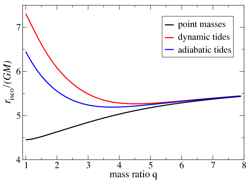
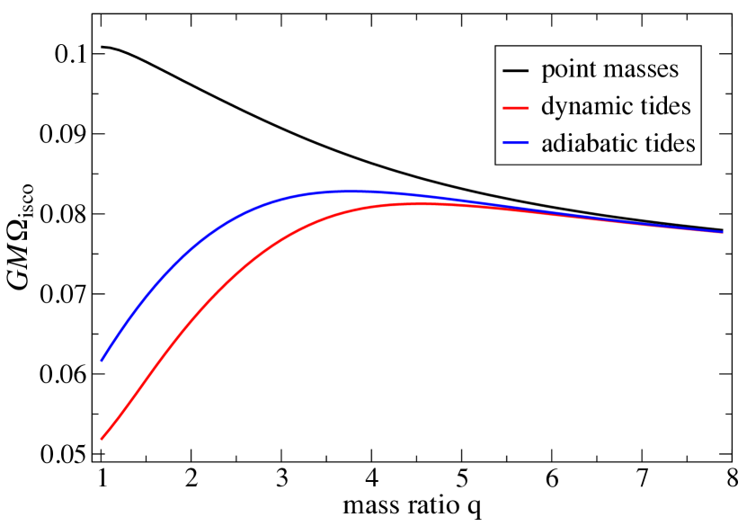
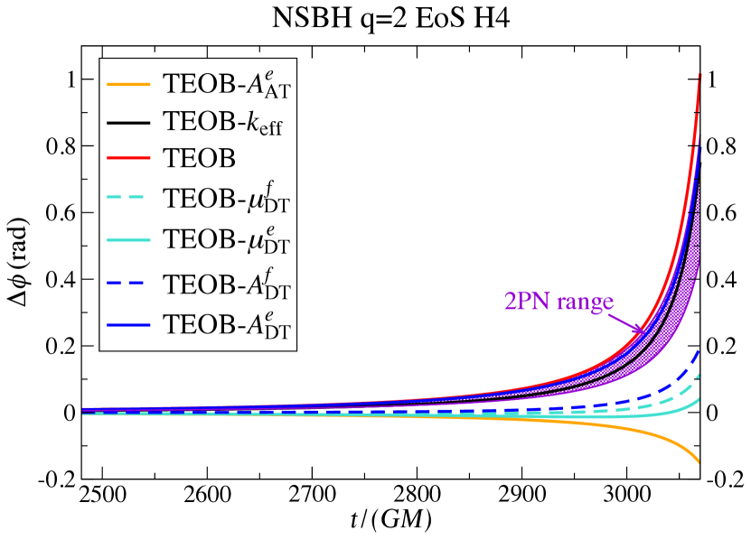
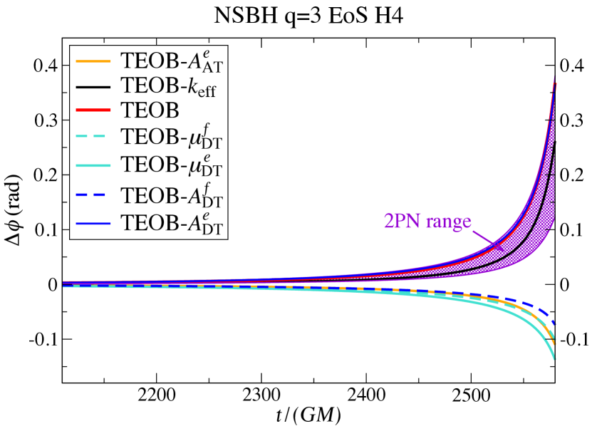
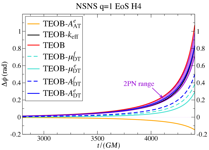
VII Results and Discussion
Before assessing the importance of dynamical tidal effects, we give more details about the EOB model used in the analysis. We only consider the circular-orbit version of all results here, since in this case more information about tidal effects at 2PN order is available. We checked that the generic-orbit version of the Hamiltonian typically differs by less than 0.1 radian from the circular-orbit version (for circular orbits at 1PN order and over 24 cycles). We fix the remaining arbitrary constant in the model in Eq. (130) to be , since this choice implies that the gauge parameters (125) are the same as for the factorized models (145). This choice can be revised once the complete 2PN dynamical result becomes available. The initial conditions for the EOB evolutions are the equilibrium solutions of the EOB equations of motion determined numerically, as explained in Appendix B.
We first consider the effect of dynamical tides in the conservative dynamics, specifically on the location of the innermost stable circular orbit (ISCO). This is shown in Fig. 3 for the case with a radius of 13.5 km and a piecewise polytropic approximation to the H4 equation of state from Refs. Read et al. (2009); Hotokezaka et al. (2013), which gives a tidal deformability of and f-mode frequency of . The plots suggest that dynamical tidal effects become important as soon as tidal effects become relevant.
However, the most interesting observables are the gravitational waves emitted by the system. To generate waveforms, we also include radiation-reaction forces constructed from the flux in Ref. Taracchini et al. (2012) together with the analytically known adiabatic tidal corrections to the waveform modes from Ref. Damour et al. (2012), as explained in detail in Ref. Taracchini et al. (2016). We evaluate the relevance of dynamical tidal effects on gravitational waves using the following models devised in the previous section: (i) the dynamical tidal model based on the EOB construction developed in Sec. VI.1 and denoted by TEOB here, (ii) the factorized models from Sec. VI.4 where tidal terms are contained exclusively in either or and denoted by TEOB-, (iii) their Taylor expanded versions TEOB-, and (iv) the “effective–Love-number” model denoted by TEOB- based on Sec. VI.5 and the adiabatic EOB model (134) from Ref. Bini et al. (2012). These models are summarized in Table 1.
The difference in the gravitational-wave phase between our dynamical tidal models and the 2PN TEOB- adiabatic tidal model from Ref. Bini et al. (2012) used as a baseline is shown in Figs. 4 and 5. Note that the span of the 2PN results lies within the 1PN results, indicating that an inclusion of even higher PN orders would refine our findings, but is unlikely to move the results in a different region. This plot also demonstrates the importance of 2PN knowledge. The 2PN results show that dynamical tidal effects are important at least up to a mass ratio of 3, in agreement with Fig. 3. It is also intriguing that the two Taylor expanded alternative models TEOB- and TEOB- lead to very different results at 1PN, but their factorized versions agree quite well. This demonstrates that the factorization can remove some arbitrariness from the EOB resummation.
We further note from Fig. 4 that the effective–Love-number model TEOB- captures the effects well, in spite of the derivation of being based on Newtonian gravity and leading-order radiation reaction. However, in hindsight this makes sense because (i) the model includes relativistic corrections to the tidal field with 2PN accuracy since the effective–Love-number function enters through Eq. (134), and (ii) the relativistic redshift and frame-dragging effects tend to compensate each other (as explained in Sec. I.2), thus leading to only a small shift of the resonance condition away from the Newtonian expectation. Since the TEOB- model does not require an evolution of additional dynamical variables it is more convenient for generating a large bank of gravitational waveforms. Furthermore, the Love number and f-mode frequency are linked by an approximately universal relation Chan et al. (2014), which can be used to reduce the parameter space for the template bank. A universality of this kind can also potentially be used as a test of general relativity, as discussed in Ref. Yagi and Yunes (2013).
Previous studies have raised concerns regarding the measurement of tidal effects due to the lack of knowledge of high-order terms in the PN approximation in the point-mass sector Favata (2014); Yagi and Yunes (2014). This is because, as discussed in Sec. III, Newtonian tidal effects enter formally at 5PN order, but the point-mass terms are only known to 4PN order, so that this lack of PN knowledge could lead to systematic errors in the measurements of tidal parameters. However, this issue arises only for PN-based analytical waveform models. It is mitigated in the EOB model since its point-mass version is resummed and calibrated to numerical relativity Taracchini et al. (2014) and thus effectively includes all the higher PN orders. For nonspinning binaries the systematic errors in the EOB model have been quantified and found to be small. Therefore, EOB-based measurements of tidal parameters for such systems are not expected to be contaminated by the large systematic errors found in Favata (2014); Yagi and Yunes (2014). This issue also illustrates why synergetic approaches like EOB are important to obtain accurate waveforms over the full frequency range of current detectors.
VIII Conclusion
In this paper we developed a general relativistic model for dynamic tides based on a covariant effective action. While we focused our analysis on the quadrupolar f-mode oscillations of neutron stars, the results can readily be extended to more general cases and higher multipoles. We derived explicit results for all the contributions to this action both in the PN and the test-particle limit and discussed the physical effects encoded in these results. This served as the foundation for constructing, for the first time, an EOB Hamiltonian describing dynamical tidal effects both for generic orbits and specialized to circular orbits. In contrast to the line of work in Refs. Bini et al. (2012); Bernuzzi et al. (2015), our TEOB model does not contain poles at the light ring due to the choice of gauge we adopted,666A comparison of our TEOB model and the models in Refs. Bini et al. (2012); Bernuzzi et al. (2015) against numerical-relativity simulations can be found in Refs. Hinderer et al. (2016); Taracchini et al. (2016). but it still reproduces the test-particle limit. Throughout these derivations we provided the relevant details of the calculations to make the paper self-contained and highlighted various subtleties. We then used the new tidal EOB Hamiltonian to show that dynamical tides are relevant both in the conservative dynamics and in the gravitational-wave phase and quantified the uncertainty in the model due to the lack of higher-order tidal PN information. Moreover, we devised a computationally more efficient yet approximate TEOB model where the dynamical tidal effects are encoded in an effective–Love-number function which we calculated.
Our model is currently being implemented for gravitational-wave data analysis and will aid in extracting the unique information on the equation of state of neutron stars from upcoming observations with Advanced LIGO and Virgo. In a forthcoming paper Taracchini et al. (2016) we will study refinements of the EOB waveform model, include dynamical higher multipoles, as well as the effects of dynamical tides in the dissipative sector and hence in the waveform amplitudes, and perform comparisons of the model against new highly accurate numerical-relativity simulations of neutron-star–black-hole binary systems.
Acknowledgements.
We gratefully acknowledge useful discussions with Justin Vines and Francois Foucart. T. H. acknowledges support from NSF Grant No. PHY-1208881 and thanks the Max Planck Institute for Gravitational Physics in Potsdam for hospitality.Appendix A Point-mass parts of the effective-one-body potentials
Here we report the point-mass potentials from Ref. Taracchini et al. (2014) that enter our tidal EOB model. The potential is given by
| (167) |
with
| (168a) | |||||
| (168b) | |||||
| (168c) | |||||
| (168d) | |||||
| (168e) | |||||
| (168f) | |||||
| (168g) | |||||
| (168h) | |||||
where is a calibration parameter tuned to numerical-relativity simulations whose value is given in Ref. Taracchini et al. (2014). The potential is
| (169) |
In all expressions above we use only the nonspinning limit where . In our implementation, we evolve the “tortoise” radial momentum
| (170) |
instead of , and for the non-geodesic term we use
| (171) |
Appendix B Equilibrium and adiabatic solutions
Equilibrium solutions are solutions for that are static in the corotating frame and exist for circular orbits. These solutions are obtained by solving for when setting to zero the time derivatives of the equations of motion: , . Here, we give the specific solutions for the variables defined in Eq. (108) for the case of our TEOB model, the generalization to other tidal resummations can be derived from the above equilibrium equations. When written out explicitly, the EOB tidal potentials in the circular-orbit limit are
| (172a) | |||||
| (172b) | |||||
| (172c) | |||||
From we obtain , and from both we find . To proceed further requires either numerically solving the equations for or making a perturbative expansion by linearizing in the tidal terms. The results of this can be obtained explicitly with Mathematica, but are not particularly illuminating. Note that when doing a PN expansion one cannot brute-force expand the full EOB solutions for since this would also PN-expand the “Newtonian” dependence (or with EOB involving rather than ). When solving the equations of motion iteratively for etc. we obtain
| (173a) | |||||
| (173b) | |||||
| (173c) | |||||
where . The adiabatic limit is obtained for or in Eqs. (173) and leads to
| (174) |
and . For the initial conditions we use the circular-orbit solution for (valid again for our TEOB model, but the generalization to other models simply requires setting to zero and or ),
| (175) |
Here , primes denote derivatives with respect to , and all tidal potentials are evaluated for the equilibrium solutions computed numerically as described above. We augment the nontrivial solutions for , , , by the initial value for . This is computed from numerically solving for from
| (176) |
Appendix C The oscillator Hamiltonian and the mapping from post-Newtonian to effective-one-body Hamiltonians
In this appendix we discuss some subtleties in the identifications of tidal terms in the EOB model that arise when starting from the structures in the PN Hamiltonian instead of basing the construction on the test-particle limit. Whereas in the test-particle case we can obtain additional information from the mass-shell constraint (see Sec. IV.2), this information is not readily available in the PN limit where our explicit results are limited to the Hamiltonian. Below we discuss the consequences of this imbalance in the source of information in the two limits. We start by outlining several arguments for adding tidal terms into the various EOB functions similar to those for the test-particle limit. While for the interaction terms both the Newtonian limit and test-particle expectations lead to consistent identifications, the oscillator terms give rise to a discrepancy that we discuss and resolve.
The structure of the leading-order PN-tidal corrections can be identified in a similar manner as discussed in the context of the test-particle, namely by counting the power of momenta in each term. First, we note that based on our assumptions, the effective metric is independent of the canonical momentum. As a consequence, the structure of Eq. (86) dictates that (i) interactions that are linear in must be incorporated in the potential , (ii) terms quadratic in should appear in , and (iii) terms independent of the momentum must be in . Remaining terms of cubic and higher order in are then collected into . Following this reasoning we deduce that the Newtonian interaction term in Eq. (III.2), which is independent of the momenta, belongs to . This agrees with the result of applying similar arguments in the test-particle case to the second term on the right-hand side of Eq. (82). However, this consistency between PN and test-particle–limit identifications fails for the oscillator piece.
We have deduced in Sec. IV B that in the test-particle limit the pure oscillator Hamiltonian enters the EOB functions through the nongeodesic term . On the other hand, following the reasoning for the EOB identification of PN corrections we note that in the Newtonian limit the oscillator Hamiltonian (57) with does not depend on the canonical linear momentum. Following the classification of terms by powers of momenta, it should therefore be included in instead of . This discrepancy is due to the additional information from the -dependence in the mass-shell constraint (25), which is available in the test-particle limit, but not in the PN Hamiltonian. This means that the test-particle limit gives a more refined picture in this case, so we include the oscillator part in here.
The freedom in making the identifications between PN tidal terms and the EOB Hamiltonian can also be exploited to devise different mappings. For instance, adopting the convention that momentum-independent terms should be included in in the PN case would shift the disagreement with the test-particle mass-shell constraint to the contributions. However, it is important to stress that these ambiguities have no physical consequences and are merely a result of incomplete information within the different approximation schemes. In particular, note that PN information enters in the oscillator Hamiltonian (57) only through the redshift . An accurate prediction for the value of the redshift beyond the PN expressions is provided by the EOB point-mass Hamiltonian through
| (177) |
Since has been calibrated to numerical-relativity simulations for circular orbits, this formula gives the redshift to high accuracy and could be used to improve the resummation of the pure oscillator terms in any of the EOB potentials.
Finally, we point out another interesting possibility for a resummation. The Hamiltonian (57) together with Eq. (177) is the first term in a Taylor expansion in the mass . The most elegant way to include the oscillator terms is therefore a shift of the mass given by
| (178) |
in . This automatically makes the oscillatory dynamics as accurate as . However, it implies that dynamical terms are introduced in the energy map (83) as well. Since the tidal effects are small, we do not further explore this proposal here, but it is worth to point out that such a modification of the energy map would lead to a noticeable structural simplification.
Appendix D Canonical transformations and the pole at the light ring
In this appendix we consider the effect of using a canonical transformation to specialize the test-particle–limit tidal Hamiltonian (76) to circular orbits. The general method was explained in Sec. V.2 and here, we only provide an illustrative example for one of the terms in the Hamiltonian. This serves to clarify the statements made in Ref. Akcay et al. (2012) that the pole at the light ring comes from a particular gauge choice and it can be eliminated through a canonical transformation. In other words, the light-ring pole should be interpreted as a coordinate singularity in the phase space.
In the test-particle limit, the generator from Eq. (98) leads to the transformation
| (179) | ||||
| (180) |
We next use this relation to eliminate from the tidal part of the test-particle–limit Hamiltonian (76) in favor of its circular-orbit value as a function of given by Eq. (138),
| (181) |
which exhibits the pole at the light ring. Note that the occurrences of in the tidal part of Eq. (76) enter both through the overall prefactor , determined from Eqs. (77) and (74), and through the interaction term in Eq. (80). This can be analyzed by working with the binomial expansion
| (182) |
where we used following from . For example, consider the term involving the second combination in (82), which enters into the Hamiltonian (76) in the form
| (183) | ||||
| (184) |
where in Eq. (184) we explicitly consider only the first two terms in the expansion of from (182). If we use
| (185) |
we can eliminate the first occurrence of from the transformed Hamiltonian
| (186) |
To remove the remaining dependence on we apply a second transformation with
| (187) |
and obtain
| (188) |
Repeating this procedure and summing the series for which we only exhibited the first two terms leads to
| (189) | |||||
| (190) |
where or . This rigorously demonstrates that simply substituting Eq. (181) into Eqs. (77) and (183) is a valid procedure to specialize to circular orbits and introduces an explicit pole at the light ring .
Furthermore, as first noticed in Ref. Akcay et al. (2012), the transformation outlined above introduces a coordinate singularity in the phase space at the light ring. Here, we made it explicit that the singularity is produced by the poles in the generator of the canonical transformation . Nevertheless, the presence of poles is not problematic as long as the light ring is not reached. An important observation is that the method of the canonical transformation works in both ways, i.e., one can also remove an explicit pole at the light ring by replacing it with a function of using Eq. (181). In the explicit example given above, this corresponds to performing the inverse canonical transformation generated by minus .
References
- Abbott et al. (2016a) B. P. Abbott et al. (Virgo, LIGO Scientific), “Observation of Gravitational Waves from a Binary Black Hole Merger,” Phys. Rev. Lett. 116, 061102 (2016a), arXiv:1602.03837 [gr-qc] .
- Abbott et al. (2016b) B. P. Abbott et al. (Virgo, LIGO Scientific), “GW151226: Observation of Gravitational Waves from a 22-Solar-Mass Binary Black Hole Coalescence,” Phys. Rev. Lett. 116, 241103 (2016b), arXiv:1606.04855 [gr-qc] .
- Aasi et al. (2015) J. Aasi et al. (LIGO Scientific), “Advanced LIGO,” Class. Quant. Grav. 32, 074001 (2015), arXiv:1411.4547 [gr-qc] .
- Acernese et al. (2015) F. Acernese et al. (VIRGO), “Advanced Virgo: a second-generation interferometric gravitational wave detector,” Class. Quant. Grav. 32, 024001 (2015), arXiv:1408.3978 [gr-qc] .
- Aso et al. (2013) Y. Aso, Y. Michimura, K. Somiya, M. Ando, O. Miyakawa, T. Sekiguchi, D. Tatsumi, and H. Yamamoto (KAGRA), “Interferometer design of the KAGRA gravitational wave detector,” Phys. Rev. D88, 043007 (2013), arXiv:1306.6747 [gr-qc] .
- Iyer et al. (2011) B. Iyer et al. (LIGO Collaboration), “LIGO-India, Proposal of the Consortium for Indian Initiative in Gravitational-wave Observations,” (2011), LIGO Document M1100296-v2.
- Fernández and Metzger (2016) R. Fernández and B. D. Metzger, “Electromagnetic Signatures of Neutron Star Mergers in the Advanced LIGO Era,” Ann. Rev. Nucl. Part. Sci. 66, 23–45 (2016), arXiv:1512.05435 [astro-ph.HE] .
- Buonanno and Damour (1999) A. Buonanno and T. Damour, “Effective one-body approach to general relativistic two-body dynamics,” Phys. Rev. D59, 084006 (1999), arXiv:gr-qc/9811091 [gr-qc] .
- Buonanno and Damour (2000) A. Buonanno and T. Damour, “Transition from inspiral to plunge in binary black hole coalescences,” Phys. Rev. D62, 064015 (2000), arXiv:gr-qc/0001013 [gr-qc] .
- Abbott et al. (2016c) B. P. Abbott et al. (Virgo, LIGO Scientific), “Properties of the Binary Black Hole Merger GW150914,” Phys. Rev. Lett. 116, 241102 (2016c), arXiv:1602.03840 [gr-qc] .
- Abbott et al. (2016d) B. P. Abbott et al. (Virgo, LIGO Scientific), “Tests of general relativity with GW150914,” Phys. Rev. Lett. 116, 221101 (2016d), arXiv:1602.03841 [gr-qc] .
- Abbott et al. (2016e) B. Abbott et al. (Virgo, LIGO Scientific), “An improved analysis of GW150914 using a fully spin-precessing waveform model,” Phys. Rev. X6, 041014 (2016e), arXiv:1606.01210 [gr-qc] .
- Cowling (1941) T. G. Cowling, “The non-radial oscillations of polytropic stars,” Mon. Not. Roy. Astr. Soc. 101, 367 (1941).
- Reisenegger and Goldreich (1994) A. Reisenegger and P. Goldreich, “Excitation of neutron star normal modes during binary inspiral,” Astrophys. J. 426, 688–691 (1994).
- Shibata (1994) M. Shibata, “Effects of tidal resonances in coalescing compact binary systems,” Prog. Theor. Phys. 91, 871–884 (1994).
- Kokkotas and Schäfer (1995) K. D. Kokkotas and G. Schäfer, “Tidal and tidal resonant effects in coalescing binaries,” Mon. Not. Roy. Astron. Soc. 275, 301 (1995), arXiv:gr-qc/9502034 [gr-qc] .
- Lai (1994) D. Lai, “Resonant oscillations and tidal heating in coalescing binary neutron stars,” Mon. Not. Roy. Astron. Soc. 270, 611 (1994), arXiv:astro-ph/9404062 [astro-ph] .
- Ho and Lai (1999) W. C. Ho and D. Lai, “Resonant tidal excitations of rotating neutron stars in coalescing binaries,” Mon. Not. Roy. Astron. Soc. 308, 153 (1999), arXiv:astro-ph/9812116 [astro-ph] .
- Lai and Wu (2006) D. Lai and Y. Wu, “Resonant Tidal Excitations of Inertial Modes in Coalescing Neutron Star Binaries,” Phys. Rev. D74, 024007 (2006), arXiv:astro-ph/0604163 [astro-ph] .
- Kochanek (1992) C. S. Kochanek, “Coalescing binary neutron stars,” Astrophys. J. 398, 234 (1992).
- Bildsten and Cutler (1992) L. Bildsten and C. Cutler, “Tidal interactions of inspiraling compact binaries,” Astrophys. J. 400, 175–180 (1992).
- Flanagan and Hinderer (2008) É. É. Flanagan and T. Hinderer, “Constraining neutron star tidal Love numbers with gravitational wave detectors,” Phys. Rev. D77, 021502 (2008), arXiv:0709.1915 [astro-ph] .
- Love (1909) A. E. H. Love, “The Yielding of the Earth to Disturbing Forces,” Proceedings of the Royal Society of London Series A 82, 73–88 (1909).
- Vines and Flanagan (2013) J. E. Vines and É. É. Flanagan, “Post-1-Newtonian quadrupole tidal interactions in binary systems,” Phys. Rev. D88, 024046 (2013), arXiv:1009.4919 [gr-qc] .
- Bini et al. (2012) D. Bini, T. Damour, and G. Faye, “Effective action approach to higher-order relativistic tidal interactions in binary systems and their effective one body description,” Phys. Rev. D85, 124034 (2012), arXiv:1202.3565 [gr-qc] .
- Kojima (1987) Y. Kojima, “Stellar resonant oscillations coupled to gravitational waves,” Prog. Theor. Phys. 77, 297–309 (1987).
- Ruoff et al. (2001) J. Ruoff, P. Laguna, and J. Pullin, “Excitation of neutron star oscillations by an orbiting particle,” Phys. Rev. D63, 064019 (2001), arXiv:gr-qc/0005002 [gr-qc] .
- Gualtieri et al. (2001) L. Gualtieri, E. Berti, J. A. Pons, G. Miniutti, and V. Ferrari, “Gravitational signals emitted by a point mass orbiting a neutron star: A Perturbative approach,” Phys. Rev. D64, 104007 (2001), arXiv:gr-qc/0107046 [gr-qc] .
- Pons et al. (2002) J. A. Pons, E. Berti, L. Gualtieri, G. Miniutti, and V. Ferrari, “Gravitational signals emitted by a point mass orbiting a neutron star: Effects of stellar structure,” Phys. Rev. D65, 104021 (2002), arXiv:gr-qc/0111104 [gr-qc] .
- Flanagan and Racine (2007) É. É. Flanagan and E. Racine, “Gravitomagnetic resonant excitation of Rossby modes in coalescing neutron star binaries,” Phys. Rev. D75, 044001 (2007), arXiv:gr-qc/0601029 [gr-qc] .
- Gold et al. (2012) R. Gold, S. Bernuzzi, M. Thierfelder, B. Brügmann, and F. Pretorius, “Eccentric binary neutron star mergers,” Phys. Rev. D86, 121501 (2012), arXiv:1109.5128 [gr-qc] .
- Landry and Poisson (2015a) P. Landry and E. Poisson, “Dynamical response to a stationary tidal field,” Phys. Rev. D92, 124041 (2015a), arXiv:1510.09170 [gr-qc] .
- Maselli et al. (2012) A. Maselli, L. Gualtieri, F. Pannarale, and V. Ferrari, “On the validity of the adiabatic approximation in compact binary inspirals,” Phys. Rev. D86, 044032 (2012), arXiv:1205.7006 [gr-qc] .
- Ferrari et al. (2012) V. Ferrari, L. Gualtieri, and A. Maselli, “Tidal interaction in compact binaries: a post-Newtonian affine framework,” Phys. Rev. D85, 044045 (2012), arXiv:1111.6607 [gr-qc] .
- Maselli et al. (2013) A. Maselli, V. Cardoso, V. Ferrari, L. Gualtieri, and P. Pani, “Equation-of-state-independent relations in neutron stars,” Phys. Rev. D88, 023007 (2013), arXiv:1304.2052 [gr-qc] .
- Dixon (1979) W. G. Dixon, “Extended bodies in general relativity: their description and motion,” in Isolated Gravitating Systems in General Relativity, edited by J. Ehlers (1979) pp. 156–219.
- Blanchet (2014) L. Blanchet, “Gravitational Radiation from Post-Newtonian Sources and Inspiralling Compact Binaries,” Living Rev. Rel. 17, 2 (2014), arXiv:1310.1528 [gr-qc] .
- Yunes et al. (2006) N. Yunes, W. Tichy, B. J. Owen, and B. Brügmann, “Binary black hole initial data from matched asymptotic expansions,” Phys. Rev. D74, 104011 (2006), arXiv:gr-qc/0503011 [gr-qc] .
- Yunes and Tichy (2006) N. Yunes and W. Tichy, “Improved initial data for black hole binaries by asymptotic matching of post-Newtonian and perturbed black hole solutions,” Phys. Rev. D74, 064013 (2006), arXiv:gr-qc/0601046 [gr-qc] .
- Johnson-McDaniel et al. (2009) N. K. Johnson-McDaniel, N. Yunes, W. Tichy, and B. J. Owen, “Conformally curved binary black hole initial data including tidal deformations and outgoing radiation,” Phys. Rev. D80, 124039 (2009), arXiv:0907.0891 [gr-qc] .
- Gallouin et al. (2012) L. Gallouin, H. Nakano, N. Yunes, and M. Campanelli, “Asymptotically Matched Spacetime Metric for Non-Precessing, Spinning Black Hole Binaries,” Class. Quant. Grav. 29, 235013 (2012), arXiv:1208.6489 [gr-qc] .
- Mundim et al. (2014) B. C. Mundim, H. Nakano, N. Yunes, M. Campanelli, S. C. Noble, and Y. Zlochower, “Approximate black hole binary spacetime via asymptotic matching,” Phys. Rev. D89, 084008 (2014), arXiv:1312.6731 [gr-qc] .
- Ireland et al. (2016) B. Ireland, B. C. Mundim, H. Nakano, and M. Campanelli, “Inspiralling, nonprecessing, spinning black hole binary spacetime via asymptotic matching,” Phys. Rev. D93, 104057 (2016), arXiv:1512.05650 [gr-qc] .
- Flanagan (1998) É. É. Flanagan, “General relativistic coupling between orbital motion and internal degrees of freedom for inspiraling binary neutron stars,” Phys. Rev. D58, 124030 (1998), arXiv:gr-qc/9706045 [gr-qc] .
- Racine and Flanagan (2005) E. Racine and É. É. Flanagan, “Post-1-Newtonian equations of motion for systems of arbitrarily structured bodies,” Phys. Rev. D71, 044010 (2005), [Erratum: Phys. Rev. D88, 089903 (2013)], arXiv:gr-qc/0404101 [gr-qc] .
- Damour et al. (1991) T. Damour, M. Soffel, and C. Xu, “General relativistic celestial mechanics. 1. Method and definition of reference systems,” Phys. Rev. D43, 3273–3307 (1991).
- Damour et al. (1992) T. Damour, M. Soffel, and C. Xu, “General relativistic celestial mechanics. 2. Translational equations of motion,” Phys. Rev. D45, 1017–1044 (1992).
- Damour et al. (1993) T. Damour, M. Soffel, and C. Xu, “General relativistic celestial mechanics. 3. Rotational equations of motion,” Phys. Rev. D47, 3124–3135 (1993).
- Damour et al. (1994) T. Damour, M. Soffel, and C. Xu, “General relativistic celestial mechanics. 4: Theory of satellite motion,” Phys. Rev. D49, 618–635 (1994).
- Hinderer (2008) T. Hinderer, “Tidal Love numbers of neutron stars,” Astrophys. J. 677, 1216–1220 (2008), arXiv:0711.2420 [astro-ph] .
- Binnington and Poisson (2009) T. Binnington and E. Poisson, “Relativistic theory of tidal Love numbers,” Phys. Rev. D80, 084018 (2009), arXiv:0906.1366 [gr-qc] .
- Damour and Nagar (2009) T. Damour and A. Nagar, “Relativistic tidal properties of neutron stars,” Phys. Rev. D80, 084035 (2009), arXiv:0906.0096 [gr-qc] .
- Kol and Smolkin (2012) B. Kol and M. Smolkin, “Black hole stereotyping: Induced gravito-static polarization,” JHEP 02, 010 (2012), arXiv:1110.3764 [hep-th] .
- Poisson (2015) E. Poisson, “Tidal deformation of a slowly rotating black hole,” Phys. Rev. D91, 044004 (2015), arXiv:1411.4711 [gr-qc] .
- Landry and Poisson (2015b) P. Landry and E. Poisson, “Tidal deformation of a slowly rotating material body. External metric,” Phys. Rev. D91, 104018 (2015b), arXiv:1503.07366 [gr-qc] .
- Pani et al. (2015a) P. Pani, L. Gualtieri, A. Maselli, and V. Ferrari, “Tidal deformations of a spinning compact object,” Phys. Rev. D92, 024010 (2015a), arXiv:1503.07365 [gr-qc] .
- Pani et al. (2015b) P. Pani, L. Gualtieri, and V. Ferrari, “Tidal Love numbers of a slowly spinning neutron star,” Phys. Rev. D92, 124003 (2015b), arXiv:1509.02171 [gr-qc] .
- Kokkotas and Schmidt (1999) K. D. Kokkotas and B. G. Schmidt, “Quasinormal modes of stars and black holes,” Living Rev. Rel. 2, 2 (1999), arXiv:gr-qc/9909058 [gr-qc] .
- Nollert (1999) H.-P. Nollert, “Topical Review: Quasinormal modes: the characteristic ‘sound’ of black holes and neutron stars,” Class. Quant. Grav. 16, R159–R216 (1999).
- Taracchini et al. (2014) A. Taracchini et al., “Effective-one-body model for black-hole binaries with generic mass ratios and spins,” Phys. Rev. D89, 061502 (2014), arXiv:1311.2544 [gr-qc] .
- Nagar et al. (2016) A. Nagar, T. Damour, C. Reisswig, and D. Pollney, “Energetics and phasing of nonprecessing spinning coalescing black hole binaries,” Phys. Rev. D93, 044046 (2016), arXiv:1506.08457 [gr-qc] .
- Damour and Nagar (2010) T. Damour and A. Nagar, “Effective One Body description of tidal effects in inspiralling compact binaries,” Phys. Rev. D81, 084016 (2010), arXiv:0911.5041 [gr-qc] .
- Baiotti et al. (2011) L. Baiotti, T. Damour, B. Giacomazzo, A. Nagar, and L. Rezzolla, “Accurate numerical simulations of inspiralling binary neutron stars and their comparison with effective-one-body analytical models,” Phys. Rev. D84, 024017 (2011), arXiv:1103.3874 [gr-qc] .
- Bernuzzi et al. (2012) S. Bernuzzi, A. Nagar, M. Thierfelder, and B. Brügmann, “Tidal effects in binary neutron star coalescence,” Phys. Rev. D86, 044030 (2012), arXiv:1205.3403 [gr-qc] .
- Bini and Damour (2014) D. Bini and T. Damour, “Gravitational self-force corrections to two-body tidal interactions and the effective one-body formalism,” Phys. Rev. D90, 124037 (2014), arXiv:1409.6933 [gr-qc] .
- Bernuzzi et al. (2015) S. Bernuzzi, A. Nagar, T. Dietrich, and T. Damour, “Modeling the Dynamics of Tidally Interacting Binary Neutron Stars up to the Merger,” Phys. Rev. Lett. 114, 161103 (2015), arXiv:1412.4553 [gr-qc] .
- Hinderer et al. (2016) T. Hinderer et al., “Effects of neutron-star dynamic tides on gravitational waveforms within the effective-one-body approach,” Phys. Rev. Lett. 116, 181101 (2016), arXiv:1602.00599 [gr-qc] .
- Taracchini et al. (2016) A. Taracchini, F. Foucart, et al., “Effective-one-body waveforms and numerical-relativity simulations of nonspinning neutron-star–black-hole binaries,” in preparation (2016).
- Goldberger and Rothstein (2006a) W. D. Goldberger and I. Z. Rothstein, “An Effective field theory of gravity for extended objects,” Phys. Rev. D73, 104029 (2006a), arXiv:hep-th/0409156 [hep-th] .
- Goldberger (2007) W. D. Goldberger, “Effective field theories and gravitational radiation,” in Les Houches Summer School - Session 86: Particle Physics and Cosmology: The Fabric of Spacetime (2007) pp. 351–353, 355–396, arXiv:hep-ph/0701129 [hep-ph] .
- Goldberger and Rothstein (2006b) W. D. Goldberger and I. Z. Rothstein, “Dissipative effects in the worldline approach to black hole dynamics,” Phys. Rev. D73, 104030 (2006b), arXiv:hep-th/0511133 [hep-th] .
- Goldberger and Ross (2010) W. D. Goldberger and A. Ross, “Gravitational radiative corrections from effective field theory,” Phys. Rev. D81, 124015 (2010), arXiv:0912.4254 [gr-qc] .
- Chandrasekhar (1964) S. Chandrasekhar, “A General Variational Principle Governing the Radial and the Non-Radial Oscillations of Gaseous Masses.” Astrophys. J. 139, 664 (1964).
- Alexander (1987) M. E. Alexander, “Tidal resonances in binary star systems,” Mon. Not. Roy. Astr. Soc. 227, 843–861 (1987).
- Gingold and Monaghan (1980) R. A. Gingold and J. J. Monaghan, “The Roche problem for polytropes in central orbits,” Mon. Not. Roy. Astr. Soc. 191, 897–924 (1980).
- Rathore et al. (2003) Y. Rathore, A. E. Broderick, and R. Blandford, “A variational formalism for tidal excitation: non-rotating, homentropic stars,” Mon. Not. Roy. Astron. Soc. 339, 25 (2003), arXiv:astro-ph/0209003 [astro-ph] .
- Chakrabarti et al. (2013a) S. Chakrabarti, T. Delsate, and J. Steinhoff, “Effective action and linear response of compact objects in Newtonian gravity,” Phys. Rev. D88, 084038 (2013a), arXiv:1306.5820 [gr-qc] .
- Press and Teukolsky (1977) W. H. Press and S. A. Teukolsky, “On formation of close binaries by two-body tidal capture,” Astrophys. J. 213, 183–192 (1977).
- Cox (1980) J. P. Cox, Theory of stellar pulsation (Princeton University Press, Princeton, NJ, 1980).
- Damour and Schäfer (1991) T. Damour and G. Schäfer, “Redefinition of position variables and the reduction of higher order Lagrangians,” J. Math. Phys. 32, 127–134 (1991).
- Chakrabarti et al. (2013b) S. Chakrabarti, T. Delsate, and J. Steinhoff, “New perspectives on neutron star and black hole spectroscopy and dynamic tides,” (2013b), arXiv:1304.2228 [gr-qc] .
- Steinhoff (2015) J. Steinhoff, “Spin and quadrupole contributions to the motion of astrophysical binaries,” Proceedings, 524th WE-Heraeus-Seminar: Equations of Motion in Relativistic Gravity (EOM 2013), Fund. Theor. Phys. 179, 615–649 (2015), arXiv:1412.3251 [gr-qc] .
- Steinhoff (2011) J. Steinhoff, “Canonical formulation of spin in general relativity,” Ann. Phys. (Berlin) 523, 296–353 (2011), arXiv:1106.4203 [gr-qc] .
- Dirac (1950) P. A. M. Dirac, “Generalized Hamiltonian dynamics,” Canad. J. Math. 2, 129–148 (1950).
- Dirac (1964) P. A. M. Dirac, Lectures on Quantum Mechanics (Yeshiva University Press, New York, 1964).
- Levi and Steinhoff (2015) M. Levi and J. Steinhoff, “Spinning gravitating objects in the effective field theory in the post-Newtonian scheme,” JHEP 09, 219 (2015), arXiv:1501.04956 [gr-qc] .
- Blanchet et al. (2013) L. Blanchet, A. Buonanno, and A. Le Tiec, “First law of mechanics for black hole binaries with spins,” Phys. Rev. D87, 024030 (2013), arXiv:1211.1060 [gr-qc] .
- Poisson (1998) E. Poisson, “Gravitational waves from inspiraling compact binaries: The Quadrupole moment term,” Phys. Rev. D57, 5287–5290 (1998), arXiv:gr-qc/9709032 [gr-qc] .
- Porto and Rothstein (2008) R. A. Porto and I. Z. Rothstein, “Next to Leading Order Spin(1)Spin(1) Effects in the Motion of Inspiralling Compact Binaries,” Phys. Rev. D78, 044013 (2008), [Erratum: Phys. Rev. D81, 029905 (2010)], arXiv:0804.0260 [gr-qc] .
- Hergt et al. (2010) S. Hergt, J. Steinhoff, and G. Schäfer, “Reduced Hamiltonian for next-to-leading order Spin-Squared Dynamics of General Compact Binaries,” Class. Quant. Grav. 27, 135007 (2010), arXiv:1002.2093 [gr-qc] .
- Levi and Steinhoff (2016a) M. Levi and J. Steinhoff, “Next-to-next-to-leading order gravitational spin-squared potential via the effective field theory for spinning objects in the post-Newtonian scheme,” JCAP 1601, 008 (2016a), arXiv:1506.05794 [gr-qc] .
- Tulczyjew (1959) W. Tulczyjew, “Equations of motion of rotating bodies in general relativity theory,” Acta Phys. Polon. 18, 37–55 (1959), [Erratum: Acta Phys. Polon. 18, 534 (1959)].
- Damour (1982) T. Damour, “Probléme des deux corps et freinage de rayonnement en relativité générale,” C. R. Acad. Sci. Paris Sér. II 294, 1355–1357 (1982).
- Damour and Schäfer (1988) T. Damour and G. Schäfer, “Higher Order Relativistic Periastron Advances and Binary Pulsars,” Nuovo Cim. B101, 127–176 (1988).
- Hartung and Steinhoff (2011) J. Hartung and J. Steinhoff, “Next-to-next-to-leading order post-Newtonian spin-orbit Hamiltonian for self-gravitating binaries,” Ann. Phys. (Berlin) 523, 783–790 (2011), arXiv:1104.3079 [gr-qc] .
- Levi and Steinhoff (2016b) M. Levi and J. Steinhoff, “Next-to-next-to-leading order gravitational spin-orbit coupling via the effective field theory for spinning objects in the post-Newtonian scheme,” JCAP 1601, 011 (2016b), arXiv:1506.05056 [gr-qc] .
- Tauber (1988) G. E. Tauber, “Canonical formalism and equations of motion for a spinning particle in general relativity,” Int. J. Theor. Phys. 27, 335 (1988).
- Vines et al. (2016) J. Vines, D. Kunst, J. Steinhoff, and T. Hinderer, “Canonical Hamiltonian for an extended test body in curved spacetime: To quadratic order in spin,” Phys. Rev. D93, 103008 (2016), arXiv:1601.07529 [gr-qc] .
- Barausse et al. (2009) E. Barausse, E. Racine, and A. Buonanno, “Hamiltonian of a spinning test-particle in curved spacetime,” Phys. Rev. D80, 104025 (2009), [Erratum: Phys. Rev. D85, 069904 (2012)], arXiv:0907.4745 [gr-qc] .
- Damour et al. (2000) T. Damour, P. Jaranowski, and G. Schäfer, “On the determination of the last stable orbit for circular general relativistic binaries at the third post-Newtonian approximation,” Phys. Rev. D62, 084011 (2000), arXiv:gr-qc/0005034 [gr-qc] .
- Damour and Nagar (2014) T. Damour and A. Nagar, “New effective-one-body description of coalescing nonprecessing spinning black-hole binaries,” Phys. Rev. D90, 044018 (2014), arXiv:1406.6913 [gr-qc] .
- Taracchini et al. (2012) A. Taracchini, Y. Pan, A. Buonanno, E. Barausse, M. Boyle, T. Chu, G. Lovelace, H. P. Pfeiffer, and M. A. Scheel, “Prototype effective-one-body model for nonprecessing spinning inspiral-merger-ringdown waveforms,” Phys. Rev. D86, 024011 (2012), arXiv:1202.0790 [gr-qc] .
- Damour et al. (2008) T. Damour, P. Jaranowski, and G. Schäfer, “Effective one body approach to the dynamics of two spinning black holes with next-to-leading order spin-orbit coupling,” Phys. Rev. D78, 024009 (2008), arXiv:0803.0915 [gr-qc] .
- Barker and O’Connell (1980a) B. M. Barker and R. F. O’Connell, “Acceleration-dependent lagrangians and equations of motion,” Physics Letters A 78, 231–232 (1980a).
- Barker and O’Connell (1980b) B. M. Barker and R. F. O’Connell, “Removal of acceleration terms from the two-body Lagrangian to order c-4 in electromagnetic theory,” Canadian Journal of Physics 58, 1659 (1980b).
- Akcay et al. (2012) S. Akcay, L. Barack, T. Damour, and N. Sago, “Gravitational self-force and the effective-one-body formalism between the innermost stable circular orbit and the light ring,” Phys. Rev. D86, 104041 (2012), arXiv:1209.0964 [gr-qc] .
- Kevorkian and Cole (2012) J. Kevorkian and J. D. Cole, Multiple scale and singular perturbation methods, Vol. 114 (Springer Science & Business Media, 2012).
- Read et al. (2009) J. S. Read, B. D. Lackey, B. J. Owen, and J. L. Friedman, “Constraints on a phenomenologically parameterized neutron-star equation of state,” Phys. Rev. D79, 124032 (2009), arXiv:0812.2163 [astro-ph] .
- Hotokezaka et al. (2013) K. Hotokezaka, K. Kyutoku, and M. Shibata, “Exploring tidal effects of coalescing binary neutron stars in numerical relativity,” Phys. Rev. D87, 044001 (2013), arXiv:1301.3555 [gr-qc] .
- Damour et al. (2012) T. Damour, A. Nagar, and L. Villain, “Measurability of the tidal polarizability of neutron stars in late-inspiral gravitational-wave signals,” Phys. Rev. D85, 123007 (2012), arXiv:1203.4352 [gr-qc] .
- Chan et al. (2014) T. K. Chan, Y.-H. Sham, P. T. Leung, and L.-M. Lin, “Multipolar universal relations between f-mode frequency and tidal deformability of compact stars,” Phys. Rev. D90, 124023 (2014), arXiv:1408.3789 [gr-qc] .
- Yagi and Yunes (2013) K. Yagi and N. Yunes, “I-Love-Q,” Science 341, 365–368 (2013), arXiv:1302.4499 [gr-qc] .
- Favata (2014) M. Favata, “Systematic parameter errors in inspiraling neutron star binaries,” Phys. Rev. Lett. 112, 101101 (2014), arXiv:1310.8288 [gr-qc] .
- Yagi and Yunes (2014) K. Yagi and N. Yunes, “Love can be Tough to Measure,” Phys. Rev. D89, 021303 (2014), arXiv:1310.8358 [gr-qc] .