Accuracy and effectualness of closed-form, frequency-domain waveforms for non-spinning black hole binaries
Abstract
The coalescences of binary black hole (BBH) systems, here taken to be non-spinning, are among the most promising sources for gravitational wave (GW) ground-based detectors, such as LIGO and Virgo. To detect the GW signals emitted by BBHs, and measure the parameters of the source, one needs to have in hand a bank of GW templates that are both effectual (for detection), and accurate (for measurement). We study the effectualness and the accuracy of the two types of parametrized banks of templates that are directly defined in the frequency-domain by means of closed-form expressions, namely ‘post-Newtonian’ (PN) and ‘phenomenological’ models. In absence of knowledge of the (continuous family of) exact waveforms, our study assumes as fiducial, target waveforms the ones generated by the most accurate version of the effective-one-body (EOB) formalism, calibrated upon a few high-accuracy numerical relativity (NR) waveforms. We find that, for initial GW detectors the use, at each point of parameter space, of the best closed-form template (among PN and phenomenological models) leads to an effectualness over the entire mass range and in an important fraction of parameter space; however, when considering advanced detectors, both of the closed-form frequency-domain models fail to be effectual enough in significant domains of the two-dimensional [total mass and mass ratio] parameter space. Moreover, we find that, both for initial and advanced detectors, the two closed-form frequency-domain models fail to satisfy the minimal required accuracy standard in a very large domain of the two-dimensional parameter space. In addition, a side result of our study is the determination, as a function of the mass ratio, of the maximum frequency at which a frequency-domain PN waveform can be ‘joined’ onto a NR-calibrated EOB waveform without undue loss of accuracy. In the case of mass ratios larger than 4:1 this maximum frequency occurs well before the last stable orbit, leaving probably too many orbital cycles to be covered by current NR techniques if one wanted to construct accurate enough hybrid PN-NR waveforms. This problem will, however, be probably greatly alleviated, or even solved, by using the EOB formalism instead of PN theory.
pacs:
07.05.Kf, 04.30.-w, 04.25.dg, 04.25.Nx,I Introduction
During the last years very significant progress has been made towards the detection of gravitational wave (GW) signals from binary black holes (BBH) coalescences. On the experimental side, current interferometric GW detectors have been operating at their design sensitivity for several years Abramovici:1992ah ; Abbott:2003vs ; Caron:1997hu ; Acernese:2006bj ; Luck:2006ug ; Tsubono:1997 ; Hough:2000 and advanced versions of these detectors (more sensitive by an order of magnitude Harry:2010zz ) are being planned and are expected to be operational in four to five years. For example, a binary [ denoting the mass of the Sun] can be detected out to distances of by initial detectors and by advanced detectors Buonanno:2009zt . On the theoretical side, one has recently obtained a good understanding of all the stages in the dynamics of coalescing BBHs and their emitted gravitational radiation thanks to a combination of theoretical techniques: (i) the early, adiabatic inspiral stage of the evolution can be described in terms of a post-Newtonian (PN) expansion up to 3.5PN order in phase and 3PN in amplitude Blanchet:2004ek ; Blanchet:2002av ; Kidder:2008 ; Blanchet:2008je ; (ii) the late inspiral, the merger and the ring-down can be computed by numerically solving Einstein’s equations Pretorius:2005gq ; Campanelli:2005dd ; Baker:2005vv ; Gonzalez:2006md ; Gonzalez:2007hi ; Pollney:2007ss ; Boyle:2007ft ; Boyle:2008ge ; Scheel:2008rj ; Hannam:2009hh ; Pollney:2009yz ; Reisswig:2009us ; Hannam:2010ec ; Pretorius:2007nq ; and (iii) the effective-one-body (EOB) formalism Buonanno:1998gg ; Buonanno:2000ef ; Damour:2000we ; Damour:2001tu has shown its capability of incorporating information coming both from PN theory and numerical relativity (NR) results into an accurate description Buonanno:2006ui ; Buonanno:2007pf ; Damour:2007yf ; Damour:2007vq ; Damour:2008te ; Damour:2009kr ; Buonanno:2009qa ; Yunes:2009ef ; Pan:2009wj of the whole BBHs dynamics and GW radiation, from the early inspiral, right across the last stable orbit, to the “plunge”, the merger and the final ringdown.
From the data analysis point of view, the detection of the GW signals emitted by BBHs necessitates the prior knowledge of ‘model waveforms’, i.e. of faithful representations of the emitted gravitational waveforms. These model waveforms are used to detect, and then to measure the properties of, a putative BBH by employing them to match-filter Helmstrom:1968 the output of the detector. As the expected GW signals depend on several continuous parameters (notably the masses of the two BHs in the non-spinning case), one needs to construct very large banks of model waveforms, in order to densely sample the multi-dimensional space of possible signals. Full NR simulations are computationally much too demanding to provide sufficiently long waveforms, for sufficiently many parameter values. Faster methods, making use of our analytical knowledge of BBHs, need to be considered for data analysis purposes. Several possibilities can be (and are being) pursued: (i) one can use PN theory by itself to construct template waveforms representing the inspiral part of the evolution; and the PN templates can be defined either in the time-domain, or the frequency-domain (see DIS:2001 for various possibilities and Buonanno:2009zt for a recent comparison of these possibilities); (ii) one can use EOB theory, calibrated to a small sample of high-accuracy NR waveforms, to construct time-domain waveforms that cover the whole BBH evolution, from early inspiral to ringdown; (iii) a third possibility is to construct closed-form, frequency-domain “phenomenological” waveform models PhenV1 ; PhenV2 ; Santamaria:2010yb ; these models are obtained by fitting some piece-wise analytical formulae to the Fourier transforms of a small sample of hybrid time-domain PN-NR waveforms.
From a data analyst point of view, an attractive feature of both the frequency-domain PN models, and the phenomenological ones, is that they are defined by closed-form expressions directly in the Fourier domain, converting the waveform generation to an extremely fast process, which is very convenient to perform extensive searches or parameter estimation studies. The EOB waveform models are obtained, in the time domain, by integrating ordinary differential equations (ODE’s) that depend on the continuous parameters of the considered BBH. Each EOB waveform can be obtained quite fast, both in the time domain, and then (using a Fast Fourier Transform (FFT)) in the frequency domain (see below for numbers). However, the exploration of variations in the continuous parameters of the source is much more time-consuming than in the case of analytic, closed-form frequency-domain models. It is therefore useful to compare the closed-form model waveforms to the NR-calibrated EOB ones. If one were to find that the closed-form frequency-domain waveforms were so close to the NR-calibrated EOB ones that they would be essentially equivalent for performing the data analysis of GW signals, there would be no need to construct large banks of EOB templates.
This raises the issue of having quantitative measures of the “closeness” of two model waveforms that directly translate into their closeness in the data analysis of GW signals. We recall that, in GW data analysis, model waveforms can be used in two different ways, either for the mere detection of the signals, and/or, after detection, for the measurement of properties of the source. In both cases one uses match-filtering Helmstrom:1968 , i.e. a convolution of the measured strain in the detector with a large bank of model waveforms. Ideally, one can and should (for consistency) use the same bank of waveforms for detection and measurement. But, as the accuracy requirements are different for detection and measurement (and are stricter for measurement), it might be advantageous, from a practical point of view, to have in hand two different banks of template waveforms. The issue of defining, in a quantitative manner that is related to data analysis, the closeness of two model waveforms has been discussed in several works DIS:1998 ; fairhurst ; lindblom:2008 ; lindblom:2009 ; lindblom:2010 , and has already been applied to comparing different models in, e.g., Refs. DIS:1998 ; DIS:2000 ; DIS:2001 ; Damour:2002vi ; Buonanno:2002ft ; Cokelaer:2004pw ; Pan:2007nw ; Buonanno:2009zt . Ref. DIS:1998 introduced a special nomenclature for referring to two particular measures of the closeness of a model waveform to a supposedly exact waveform: (i) the effectualness (related to the maximum signal-to-noise ratio (SNR) associated to the use of a bank of model waveforms); and (ii) the faithfulness (measuring the SNR associated to a model waveform having the same physical parameters as the exact one). The effectualness is a useful measure for detection purposes, and we shall use it below. The faithfulness was defined as a quantitative way of gauging the quality of a model waveform for measurement purposes. The recent literature fairhurst ; lindblom:2008 has emphasized that, for measurement, there is a better, data-analysis-relevant, measure of the closeness of a model waveform to a supposedly exact one, namely the Wiener (noise-weighted) squared distance between the two waveforms. Below, after discussing the motivation for the use of this measure, we shall introduce a certain related quantity that we shall call the inaccuracy of a model waveform (with respect to a supposedly given exact waveform). Then, we shall use this inaccuracy to gauge the quality of the closed-form, frequency-domain model waveforms. [We shall also see that, in most cases, the ‘inaccuracy’ is essentially proportional to the “unfaithfulness” .]
The aim of this paper is to study, by means of the two data-analysis relevant measures of effectualness and (in-)accuracy, the two classes of closed-form, frequency domain waveform models for non-spinning BBH systems, namely PN expansions and phenomenological waveforms. There remains, however, to discuss the issue of the choice of supposedly exact target waveforms. In absence of knowledge of the (continuous family of) exact waveforms, our study will assume as fiducial, target waveforms the ones generated by the most accurate version Damour:2009kr of the effective one body formalism, calibrated upon a few high-accuracy numerical relativity waveforms. We recall that Refs. Damour:2009kr ; Buonanno:2009qa have shown that, after calibration of a few EOB “flexibility” parameters onto some nonperturbative information extracted from high-accuracy NR results, the EOB waveforms exhibited an excellent agreement (within numerical errors) with state-of-the-art NR waveforms, for several mass ratios (1:1, 2:1 and 3:1). One is therefore justified in considering the two-parameter family of NR-calibrated EOB waveforms as our current best approximation to the (unknown) continuous family of (non-spinning) exact waveforms. Independently of this argument, it is anyway (as already said above) interesting to discuss, in quantitative terms, the closeness between the bank of closed-form waveforms, and the bank of EOB ones. Given the small computational time required for each EOB simulation, we shall be able to exhaustively explore the whole parameter space, and to identify the regions where the closed-form models lack in effectualness or accuracy. In the process, we shall also describe how to construct frequency-domain hybrid EOB waveforms by joining (in a smooth manner) an early-inspiral, closed-form frequency-domain PN waveform, to a subsequent Fourier-transformed EOB waveform. This will lead us to discussing the maximum frequency where the “junction” can take place without undue loss of accuracy.
This paper is organized as follows: in Sec. II we briefly review the basic concepts and definitions used in GW data analysis and discuss the accuracy standards that will be used in the rest of the paper. Section III summarizes the structure of the closed-form waveform models considered in our study, mainly with the purpose of establishing a common notation. In Sec. IV we define the time-domain EOB models we use, and describe the computation of their Fourier-transform, as well as a procedure for constructing hybrid PNEOB waveforms in the Fourier domain. Then, in Sec. V we study what is the maximum frequency value where the joining (in the frequency domain) between the early PN waveform and the subsequent EOB one can be done without undue loss of accuracy. The main results of the paper, concerning quantitative measures of the closeness between closed-form models, and EOB ones, are presented and discussed in Sec. VI. Finally, Sec. VII presents our conclusions and Sec. VIII the pointers for future work.
Also, let us note that we generally use units such that . In addition, when dealing with the EOB dynamics, and Fourier transform, we shall often use (without warning) the adimensionalized time .
II Detecting gravitational wave signals into the noise
In this section, we start by providing a brief review of the basic concepts and definitions used in GW data analysis, mainly to establish our notation. Then we give the definition of the two quantitative measures (effectualness and inaccuracy) that we shall use to quantify the accuracy of approximated waveform models in comparison with some (fiducial) exact waveform. All our derivations will be done assuming observations from a single GW detector, although they could be easily generalized to multiple detectors.
II.1 Conventions and notation
The measured strain in an interferometric GW detector, , is a time series data consisting in the combination of the detector noise, , and the exact GW signal that we want to detect, (here, and in the following, the subscript stands for “exact”). By assuming additive noise, we have
| (1) |
Commonly, the noise is modeled to be zero-mean, Gaussian and stationary, and is characterized by its (one-sided) power spectral density (PSD), , which is defined as
| (2) |
Here, the overline denotes the ensemble average, the superscript star indicates complex conjugation, and the tilde denotes the Fourier transform,
| (3) |
Note that we use here the LIGO Scientific Collaboration (LSC) sign convention for the Fourier transform, with a factor . This sign convention is opposite to the one used in many early GW papers (such as Refs. DIS:1998 ; DIS:2000 ; DIS:2001 ) which used the (theoretical-physics) convention . This change of convention introduces several sign changes in key formulas, that we shall indicate below. [Let us warn in advance the reader that, because of this, there are sign errors in some of the recent GW literature (such as AISS_2005 ).]
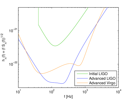
In this paper, we shall consider three different ground-based detectors: Initial LIGO, Advanced LIGO and Advanced Virgo. Following Ref. Ajith:2009fz , the one-sided noise PSDs of these detectors is approximated by some simple analytic expressions of a dimensionless frequency (see Fig. 1). For Initial LIGO, Hz, and (using a low frequency cut-off, Hz)
| (4) | |||||
For Advanced LIGO, Hz, and (using Hz)
| (5) |
For Advanced Virgo, Hz, Hz and
| (6) | |||||
Let us note here that the initial LIGO noise PSD corresponds to the one in the Science Requirements Document, which is very close to (but not the same as) the actual noise curve obtained during LIGO’s S5 and S6 science runs. The noise PSDs that we use for advanced detectors are also slightly different to the ones currently considered by the LSC and Virgo Collaboration (see Fig. 2 of Ref. Abadie:2010cfa ).
See Fig. 1 for a plot of these three PSDs in the form of the dimensionless effective GW noise . We recall that is a useful measure of the noise in that, together with the corresponding dimensionless frequency-domain effective GW signal , it yields the squared SNR as an integral over the logarithmic frequency: DIS:2000 .
The assumed Gaussianity of the noise naturally leads to the definition of an inner product (Wiener scalar product) between two (real) time series, and , namely
| (7) |
This Wiener scalar product is real and symmetric. The associated norm, say
| (8) |
is positive definite, and endows the space of (real) signals with an Euclidean structure.
Moreover, the normalization of this norm is such that the probability of having the realization of a particular noise series is . From this definition, the Neyman-Pearson criterion leads to an optimal search statistic equivalent to the form (Wiener filter), cf. Eq. (A24) of Ref. Cutler:1994ys . Here, we are using a hat to denote normalized templates , so that . By analogy with the usual Euclidean space, the inner product between two normalized signals, say , varies between and and can be thought of as defining the cosine of the “angle” between the two corresponding “unit vectors”. One often refers to this cosine as being the “overlap” between the two normalized signals, say
| (9) |
As we do not know the exact signal , but only some approximate model of it, say (where the subscript stands for ‘model’), one uses as practical search statistic the quantity . In presence of a non-zero signal within the detector strain signal , the latter quantity is the sum of a zero-mean random Gaussian variable, say (filtered noise) and of the non-random “filtered signal”, , defined as,
| (10) |
Because of our use of a normalized template it is easily checked that the zero-mean random Gaussian variable has a variance equal to unity. Therefore, the filtered signal, , represents the mean signal-to-noise ratio (SNR) for the detection of a GW signal within the detector output , when using as model template. The optimal SNR will be obtained when the template used is the exact signal that we want to detect, i.e.
| (11) |
In general, we can represent a complex gravitational wave signal in the Fourier domain in its polar form as
| (12) |
where the amplitude and the phase are real quantities. Since we are considering here real signals, we have , which implies that the amplitude and the phase are, respectively, even and odd functions of the frequency. Note that here we have explicitly introduced a minus sign in the phase to ensure, in view of the (LSC) sign convention Eq. (3) in the definition of the Fourier transform, that (with ) is, in the stationary phase approximation (SPA), the Legendre transform of the time-domain phase (modulo ): , with . This has the advantage that the so-defined frequency-domain phase then coincides (possibly modulo) with the SPA phase used in many other papers (such as DIS:2000 ; DIS:2001 ). The reader should be wary of possible errors in the literature due to the change in the sign convention for the Fourier transform, as many early papers used the theoretical-physics convention.
Note, for future use, that, in terms of real amplitudes and phases, the Wiener products and read
| (13) | |||||
Before proceeding to the definition of the accuracy standards
of a particular waveform model, let us spell out the notation we shall use for the different
waveforms that will enter our analysis:
Exact waveform
Model waveform having the same physical parameters as
Model waveform having parameters that maximize the overlap with
Model waveform of a certain discrete template bank having a maximum overlap with
.
Finally, let us mention that we shall be neglecting here the eventual calibration errors from the detectors. Taking them into account would imply a strengthening of the accuracy standards discussed below (see lindblom:2008 ).
II.2 Effectualness of model waveforms
Any modeled waveform represents an approximation to the real gravitational wave pattern that is emitted in nature, so that the practical search statistic will necessarily be less efficient in detecting a signal than the optimal Wiener filter . In GW searches, one says that is an effectual model of the exact signal if it allows for a successfull detection of the presence of a GW signal in the detector output, even if the values of parameters entering are not close to the real values of the parameters entering the exact signal . [One sometimes even allow the parameters of to take physically unrealizable values.] Following DIS:1998 , we shall quantify the effectualness, say , of a continuous (multi-parameter) bank of model waveforms by considering the maximum value of the ratio between the SNR, , obtained by using as filter, and the optimal SNR, , obtained by using the exact Wiener filter , i.e.
| (14) |
where we recall that stands for the normalized waveform in the continuous bank of models that maximizes the overlap with the exact (normalized) signal. In other words, if we represent the set of parameters that characterize our model by the vector ; is such that
| (15) |
In geometrical language, this means that the cosine of the angle (in Wiener’s signal space) between the unit vector and any unit vector in the continuous bank is maximized111Rigorously speaking we should be talking about a supremum rather than a maximum, as there is no mathematical guarantee, for a continuous bank, that the supremum is reached for some model. Anyway, in practice one always uses discrete banks where the maximum will be attained by some model. by the unit vector . This maximum cosine, corresponding to a minimum angle, will necessarily range between and , and in practice will be close to, but strictly smaller than, .
In this paper, we will restrict the source parameters to take values with real physical interpretation. In particular, the symmetric mass ratio, , will be constrained to be . [Otherwise, we would be considering systems with imaginary individual masses, and !]
It is also convenient to work with the ineffectualness, i.e. the quantity complementary (with respect to 1) of the effectualness, say . In other words, the ineffectualness of a continuous bank of models in detecting a certain exact signal is given by
| (16) |
In choosing an upper bound on the value of the ineffectualness one must, however, remember that, in practice, one approximates the continuous bank of model templates by some finite, discrete template bank. The closeness of a discrete bank to its continuous version is measured by the so-called minimal match (MM) Owen:1995tm , i.e. the minimum overlap between any model in the continuous bank, and any model in the discrete bank. One can replace the minimal match by its complementary, i.e. the maximal mismatch . It is easily seen (by viewing the complementaries of overlaps, , as squared distances between nearby points on the Wiener sphere of unit signals) that, when setting thresholds on the ineffectualness of the discretized version of a template bank (say, ), one should replace the continuous ineffectualness by the “effective” ineffectualness lindblom:2008
| (17) |
Since in any GW observation, the distance to the source is inversely proportional to the observed SNR and the number of events is proportional to the observable volume, we can express the fractional loss of potential events in terms of the effective ineffectualness of a given discrete template bank,
| (18) |
A threshold on the allowed fraction of missed events will set up the effectualness condition for any approximated template bank. Typically, one works with template banks with a maximal mismatch 222The choice of this value depends on the computational cost to generate the resulting total number of templates and the maximum false alarm rate allowed for the search., , of CBC_search_1 ; CBC_search_2 ; CBC_search_3 ; CBC_search_4 and allow for a fraction of missed events smaller than , which making use of Eq. (17), translates to the following effectualness condition,
| (19) |
In view of the fact that it is much more difficult, and expensive, to improve the sensitivity of the detectors than the quality of the template banks, one should aim at imposing on a bound significantly stricter than that corresponding to a loss of of the hard-won potential events. Then, if we assume the reasonable condition that the two contributions on the r.h.s. of Eq. (17) are comparable, i.e. , we see that we should really aim at imposing bounds on the effectualness which are on the stricter side of the condition above.
Let us end this section by a brief discussion of the procedure we used to compute the effectualness, i.e. to maximize the overlap over all the parameters entering the model waveform . There are two types of parameters we should maximize upon: (i) the physical parameters of the source (which, in the present case, are the two masses , or equivalently the total mass and the symmetric mass ratio ); and (ii) some kinematical parameters. In the present case, the relevant kinematical parameters of are some time origin , and some initial phase .
Among these parameters, the only one upon which we can maximize analytically is the arbitrary phase . Note first that, in the following, we shall work with a given target waveform (including a quasi-random initial phase), so that our problem here is only to maximize over the phase of the template waveform . [See appendix B of DIS:1998 for the case where one varies the initial phases of both the template and the target.] To do this we start by noting a simplifying feature of the frequency domain, with respect to the time domain. In the frequency domain, shifting the phase of any waveform simply corresponds to adding an arbitrary constant, say , to the phase . A look at the explicit form Eq. (13) of the Wiener scalar product shows that two waveforms whose frequency-domain phases , only differ by are orthogonal to each other. [This property does not hold in general when shifting time-domain phases by ; except when: (i) one considers just one harmonic, and (ii) the signal is such that the stationary phase approximation is accurate, see Sec. III.1.] In addition, two waveforms having the same frequency-domain amplitude have the same Wiener squared length . This shows that the two model waveforms define an equal-length, orthogonal basis of the two-plane spanned by all the phase-shifted models . Moreover, a generic phase-shifted model can be written as . These properties allow one to compute the analytical dependence upon of the scalar product of with any given waveform :
| (20) |
With this, one can maximize analytically over , with the result
| (21) |
On the other hand, the maximization over the other parameters must be done numerically. There is, however, a simplification when dealing with the maximization with respect to the time origin . Indeed, the dependence on the time origin is known analytically, so that there is, in particular, no need to recompute the full waveform every time we need to shift a time origin. Indeed, we have for the phase difference between any two waveforms
| (22) |
where . Then, it is just a matter of numerically maximizing the integral of given by Eq. (13) over .
II.3 Accuracy standards for a model waveform
Gravitational wave observations will open a new observational window on the Universe. In order to do actual astrophysics with GW, we need not only to detect signals, but also to extract reliable physical information out of them. In other words, we need to have at hand waveform models that are close enough to the exact signals to allow for an accurate enough measurement of the physical properties of the GW source. [As mentioned above, here we could be talking either about the same template bank used for detection, or about a complementary template bank used for analyzing in detail signals having passed a first detection threshold.] It has been recently emphasized fairhurst ; lindblom:2008 ; lindblom:2009 that a simple accuracy standard ensuring that a model waveform can be used for extracting most of the scientific content of the GW signal (buried within the detector noisy output ) is that the Wiener squared distance between and be smaller than one:
| (23) |
where the overline denotes the ensemble average. Here it is understood that and share the same physical parameters. [But, one is allowed to vary purely kinematical parameters such as an initial time and an initial phase .]
There are several ways of thinking about the meaning of the inequality Eq. (23). Ref. lindblom:2008 motivates it by considering the accuracy with which one can measure the parameter gauging the affine distance along a straight line connecting to in Euclidean Wiener space: . Assuming Gaussian noise, the variance of the measurement of is found to be given by
| (24) |
Therefore, the inequality (23) implies that the error in is larger than its variation when it interpolates between the two models, .
Another way of motivating Eq. (23) is to think in terms of the Wiener geometry of signal space. If the detector were noiseless, a measurement of the detector output would give us the exact location, in signal space, of the incoming signal , namely . However, the presence of noise in the detector is introducing a certain uncertainty in our knowledge of . More precisely, under our assumption of Gaussian noise, the probability distribution, in signal space, of the measured signal is . Therefore, at, say, the % probability level, our knowledge is only that the exact signal lies somewhere within a “unit ball” in Wiener space, centered around the observed signal : . The maximum knowledge we can extract from the GW data about the parameters of the source is therefore that , with . However, we do not know the exact form of the functional dependence of the signal upon the source parameters , i.e. the function . We only know an approximation of this functional dependence, namely the one given by the waveform model . By using the triangular inequality in (Euclidean) Wiener space, we can write the inequality
| (25) |
This inequality shows that the condition Eq. (23) is such that, in the worst case333As we are discussing the case where we have only one observed datum , one cannot use the fact that “on average” is centered around to try to get a better general inequality on the distance between and ., it degrades our knowledge on the values of the source parameters by being equivalent to doubling the noise level of the detector. Let us recall that our only knowledge about the source parameters is derived from the fact that the measured signal satisfies , so that it is the noise level in the detector which determines the statistical errors in parameter estimation. Therefore, a doubling (in the worst case) of the noise will add systematic biases to measured parameters of the same order as the statistical errors. This is clearly the minimal requirement we should put on the difference between and . However, as in the discussion above of the threshold for effectualness, we should remember that it is much more difficult, and expensive, to improve the sensitivity of the detectors than the quality of the template banks. Therefore, we should not allow the lack of accuracy of waveforms to lead to any significant (effective) increase of the detector noise level. In other words, we should strengthen the condition (23) into a condition of the form
| (26) |
where must be chosen so as to limit the effective increase of the noise level on the r.h.s. of the triangular inequality Eq. (II.3) to an acceptable level. Note indeed that the r.h.s. of Eq. (II.3) now reads . One should take at least , and probably or more444Note that, according to Ref. lindblom:2009b , the consideration of calibration errors in GW detectors also lead to suggesting a strengthening of the original condition Eq. (26) by a factor smaller than one. But such a ‘calibration factor’ should be taken on top of the one of Eq. (26), which has a different motivation. In other words, one should use a “safety factor” .. Only with such small values of can we really consider as being effectively indistinguishable from .
II.4 Definition of an inaccuracy functional
It is useful to rewrite the accuracy condition Eq. (26) in a different form, which highlights its connection with the faithfulness functional, , introduced in DIS:1998 . The l.h.s. of Eq. (26) depends on the absolute magnitudes of the signals (and therefore on the distance to the source). It also depends on the normalization of the Wiener metric, i.e. on the overall normalization of the PSD of the noise. Let us instead define the following functional of and :
| (27) |
We shall call the inaccuracy of the model waveform with respect to 555Note that this inaccuracy functional is not a symmetric function of its two arguments. One could also consider defining the symmetric functional obtained by replacing in Eq. (27) the denominator by . However, this would lead to an upper limit on this symmetric functional which differs from the inverse squared SNR by a factor involving the ratio .. The functional remains invariant both when one multiplies and by a common factor, and when one multiplies the noise density by an arbitrary factor. In other words, it depends only on the shape of the noise PSD, and on the relative shapes of the two waveforms and . As explicitly indicated, both waveforms refer to the same values of the physical parameters of the source. However, we can still maximize over the kinematical parameters of the waveform model , namely some arbitrary time origin , as well as some initial phase .
Using the identity
| (28) |
valid in any Euclidean space (with denoting the angle between the two vectors), we can write more explicitly the inaccuracy functional in the following expanded form
| (29) |
With this notation, the accuracy condition Eq. (26) can now written in the following form
| (30) |
where denotes the squared SNR. This reformulation of the accuracy condition has several useful features:
-
•
All the dependence on the absolute magnitudes of both the signals and the noise is rejected to the r.h.s., and in a very simple form involving the (squared) SNR. This allows one to compute the ‘inaccuracy’ on the l.h.s. from the shapes of the signals and the shape of the noise PSD independently from the various accuracy thresholds set by the r.h.s.
-
•
The inaccuracy , Eq. (29), is seen to consist of the sum of two positive-definite contributions: (i) the first one depends only on the ratio of the Wiener squares of the two signals (and vanishes when ); while (ii) the second one is proportional (and nearly equal) to twice the ‘unfaithfulness’, , where DIS:1998 . Note that, using the explicit frequency-domain expression of the inner product in terms of the amplitudes and phases of the waveforms, Eq. (13), the first contribution to the inaccuracy only depends on the frequency-domain amplitudes, and , and vanishes when they coincide; whereas the second contribution, proportional to , vanishes when both the amplitudes, and the phases and coincide.
-
•
Note in passing that if, instead of evaluating for the same values of the physical parameters, one were considering the analog of the ‘effectualness’ , i.e. if one were minimizing over the physical parameters of the model waveform, the minimization over the effective distance of would require the condition (because of the positive-definite character of the first contribution (i)), so that would reduce to the ‘ineffectualness’ .
-
•
In our comparisons below, our experience has been that the inaccuracy contribution from the amplitude differences was typically several orders of magnitude smaller than the one from the phase errors. This means that the accuracy condition Eq. (26) is practically equivalent to the following faithfulness condition
(31) -
•
If (as in lindblom:2008 ; lindblom:2009 ) we expand the inaccuracy to leading order in the amplitude and phase differences, , , it becomes
(32) where the angular brackets denote an average with respect to the normalized measure entering the squared SNR, i.e. , with the normalization factor chosen so that . This expanded expression is too coarse to be numerically useful, but it is useful in indicating that the accuracy condition Eq. (26) essentially means that
(33) i.e. that the noise-weighted quadrature sum of the fractional amplitude discrepancy and of the phase discrepancy (between and ) must be smaller than . [As we shall further discuss below, this motivates one to considering as an effective SNR.] If, for instance, we consider a SNR of and take (corresponding to an effective SNR ), we see that the accuracy condition is restricting the noise-weighted quadrature sum of the fractional amplitude discrepancy and of the phase discrepancy to be smaller than (i.e. 5 % or 0.05 radians). Such a constraint is more difficult to satisfy for the phase (for which any error in its dynamical description is accumulated over many GW cycles).
In summary, we shall require of any model waveform that it satisfies the following conditions: (i) for detection the effectualness condition Eq. (19); and (ii) for measurement the accuracy condition Eq. (30), where the inaccuracy functional is defined by Eq. (27), or, in more explicit form, by Eq. (29). From its r.h.s. we see that the higher the observed SNR, , is, the more restrictive the accuracy condition becomes. In addition, one must choose some to guarantee that the inaccuracy of the model waveform only increases the detector noise by a factor remaining close to 1.
III Closed-form, frequency-domain waveform models considered in our study
In this paper we consider GW observations from a single interferometer, assuming the detected signals to be short enough so that the orientation of the detector (due to Earth’s motion) can be considered constant during the time it is being observed. [For simplicity, we shall also not explicitly write down the (Doppler) effect on the GW signal coming from the relative motion (and cosmological redshift) between the detector and the source.] These approximations are commonly used for first and second generations of ground-based detectors, and will allow us to reduce all the dependence on the sky location, luminosity distance, polarization and inclination angles to an effective distance parameter, (see Eq. (36) below), and to an additional phase shift (see Eq. (37) below). Moreover, we shall only consider the dominant mode from the spin-weighted spherical harmonics decomposition of a signal from a non-spinning coalescing binary system.
In a suitable frame adapted to the quasi-circular orbit of the considered compact binary system, the two orthogonal polarizations of the emitted time-domain quadrupolar GW signal read
| (34) |
The relative weight between the polarizations depends on the inclination angle, , i.e. the angle between the angular momentum of the system and the propagation direction. The time series and define the (time-domain) amplitude and phase of the quadrupolar waveform. [The time-domain phase is conventionally defined so that it increases with time.]
The corresponding GW signal seen in the detector will be given by a single time series strain, , resulting from the projection of the two GW polarizations with the beam antenna patterns, and , which depend on the sky location of the source (i.e. the relative orientation of the line of sight and the normal direction of the detector’s plane) and the polarization angle Thorne:300yr . Using basic trigonometric relations, the detected strain can be written as a single cosine function, with amplitude and phase , as follows:
| (35) | |||||
where we defined
| (36) | |||||
| (37) |
If we were considering observations from multiple detectors, the amplitude and phase differences between the various detected strains would involve different and values through the antenna patterns of each detector, and thereby we could infer the sky location and polarization angle of the source. Also if we were observing a GW signal for a long time period, the time dependence of these three parameters could be used to estimate the position of the source. In this paper, we are considering short-lived signals detected by a single interferometer and therefore and will be numerical constants and absorbed, respectively, into an effective distance and the initial phase of the signal.
In the Fourier domain, the measured GW signal can be represented generically in the polar form Eq. (12). In what follows, we shall describe the different waveform models considered in our study in terms of the frequency-domain amplitude and phase, and .
III.1 Frequency-domain Post-Newtonian model: PN(f)
In the limit where the two coalescing compact objects are still far away from the merger, the post-Newtonian approximation to Einstein’s theory provides an accurate representation of the dynamics and radiation of the system. For non-spinning black holes binaries, the time-domain phase, , is known up 3.5PN order and the amplitude, , up to 3PN Blanchet:2004ek ; Blanchet:2002av ; Kidder:2008 ; Blanchet:2008je .
A closed-form expression for the PN waveform in the Fourier domain can be obtained by making use of the Stationary Phase Approximation (SPA). Using this approximation is not an extra assumption beyond the usual ones underlying the PN method. Indeed, the derivation of the time-domain PN phasing already assumes that the inspiral is adiabatic, which is the basic assumption needed for using the SPA. More precisely the SPA is valid when the amplitude and frequency of the signal evolve on time scales much longer than the orbital period: and . For a coalescing binary system the time scale of evolution of the GW amplitude and frequency is the radiation-reaction time scale so that [ being the PN expansion parameter ] stays much smaller than one essentially up to the end of the inspiral. See Droz:1999qx ; DIS:2000 for a more detailed discussion of the applicability of the SPA, and for the calculation of the first correction to the leading-order SPA. Here we shall use the leading-order SPA which has the following expression in terms of the time-domain GW amplitude , the GW phase , and the derivative of the GW frequency :
| (38) |
Here is the saddle point defined as the instant when the GW frequency is equal to the Fourier-domain argument . It is obtained by solving the equation in .
By inserting in the general SPA expression (38) the time-domain PN expressions one can obtain a closed-form expression for the PN-approximated frequency-domain inspiral waveform. As discussed in DIS:2001 there are actually several different ways of using the PN information to define . Here, we shall consider the most straightforward way of doing so (called ‘TaylorF2’ in DIS:2001 ), consisting in expanding both the frequency-domain amplitude and phase in powers of the PN expansion parameter . We recall that denotes the total mass of the system ( and being the individual masses), and the symmetric mass ratio. In the following, we shall denote simply as , but one must remember that it is a function of the Fourier variable . For brevity, we shall refer in the following to this PN-expanded frequency-domain waveform as ‘PN(f)’. We can write it as
| (39) |
where we introduced a frequency-domain cut-off at the Schwarzschild-like Last Stable Orbit (LSO) frequency ( denoting Heaviside’s step function).
The angular argument in Eq. (39) is given by the PN series
| (40) |
where and represent some arbitrary time and phase shifts. [We absorbed the SPA phase shift into .] The explicit expressions of the PN expansion coefficients (up to 3.5PN) can be identified from Eq. (3.18) of Buonanno:2009zt . [Notice that Ref. Buonanno:2009zt uses the opposite sign convention for the Fourier transform, which translates into a global sign in the frequency-domain phase , usually written explicitly in the definition of so that has the same expression with both sign conventions; compare, for instance, Eq. (12) with Eq. (3.17) of Buonanno:2009zt .]
In many early GW papers, the GW amplitude was taken only at leading order in the PN expansion, i.e. at the ‘Newtonian’ (frequency-domain) approximation:
| (41) |
Here we have kept an explicit negative sign coming from the second derivative of a complex exponential function, and we have defined the effective distance which absorbs all the sky position, polarization angle and orientation dependencies, see Eq. (36) above. The 3PN correction to the (quadrupolar) frequency-domain amplitude is then obtained by combining the 3PN-accurate expression of Kidder:2008 with the 3PN expansion of (given, e.g. , in Buonanno:2009zt ). Re-expanding the result as a single PN series leads to
| (42) | |||||
Note that, contrary to the convention generally assumed in the rest of the paper, this ‘3PN amplitude’ contains some (small) imaginary contributions (as in Kidder:2008 ). When, in the following, we shall talk about the amplitude of the PN(f) waveform we shall mean the modulus . Correlatively, when we shall talk about the phase of the PN(f) waveform we shall mean (minus) the argument of the complex number , defined in Eq. (39) (i.e. minus the argument of ).
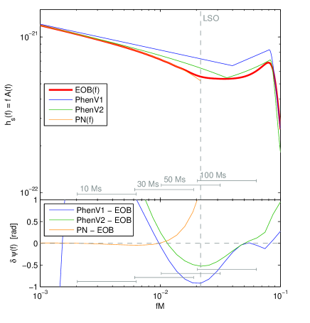
Contrary to the time-domain amplitude , which is dimensionless, the amplitude of a Fourier-transformed GW signal has the dimension of a time. By contrast, the effective GW signal amplitude is dimensionless. As dimensionless quantities, the effective amplitudes of the signal, , and of the noise, , are not affected when one rescales the frequency, by means of the total mass , into the dimensionless variable . As mentioned above, the SNR2 is given by the logarithmic frequency integral: . The effective GW amplitude of the PN(f) waveform is represented (for the equal-mass case ) in Fig. 2. This figure also plots the effective GW amplitudes of the other waveforms we shall use in the present study: the EOB one, and the two phenomenological ones that we shall introduce next. Fig. 2 represents also the difference between the phase of the PN(f) signal, and that of the corresponding EOB(f) signal. This figure indicates that both the amplitude and the phase of the PN(f) waveform stay close to that of the EOB signal up to a frequency , after which they start to deviate quite strongly. For reference, note that the GW frequency at the ‘Schwarzschild-like’ LSO is equal to , while the GW frequency at the adiabatic-EOB LSO is, for , approximately larger, being equal to . In other words, the PN(f) model starts to strongly deviate from the EOB(f) model at a frequency smaller by a factor two than the adiabatic-EOB LSO frequency. Later we shall study in more detail after which frequency the difference between PN(f) and EOB(f) starts to introduce an unacceptable level of ‘inaccuracy’ (in the technical sense defined above).
Finally, note that the horizontal segments near the bottom of the two panels of Fig. 2 indicate (for each quoted total mass ) the shortest frequency intervals upon which 70 % of the SNR for an inspiral signal () is accumulated. Here we used the Adv. LIGO PSD, and found that Hz and Hz span the shortest interval such that , with .
III.2 Non-spinning phenomenological waveform model (PhenV1)
In this paper we shall consider two different phenomenological models. [See, however, the concluding section for additional results concerning a recently published, third phenomenological model.] The first model was built by Ajith et al. PhenV1 by starting from time-domain, hybrid non-spinning waveforms in the mass-ratio range, . These time-domain hybrid waveforms were constructed by joining together, in the time domain, some early 3.5 PN TaylorT1 restricted waveforms with relatively short ( inspiral cycles, plus merger) subsequent numerical waveforms generated by the Jena group using their bam code BAM1 ; BAM2 with fourth-order finite differencing. Afterwards, the resulting phenomenological model was tested against some other hybrid waveforms built from longer and more accurate numerical simulations produced using the ccatie Pollney:2007ss and the same bam code employing sixth-order finite differencing. These time-domain hybrid waveforms were then Fourier-transformed, and the resulting sample of frequency-domain waveforms was then fitted to some piecewise-continuous multi-parameter analytic expressions, which define the closed-form ‘version-1 phenomenological waveform’, say
| (43) |
The phenomenological waveforms are defined directly in the Fourier domain: the amplitude, , is defined as a piecewise function distinguishing inspiral, merger and ring-down stages, while the phase666Notice the explicit change of sign of the phenomenological phase defined in PhenV1 compared with our definition here, Eq. (12)., , is defined as a PN-type series with phenomenological coefficients. The whole waveform is characterized by phenomenological parameters ( for the amplitude and for the phase), each of them fitted to a quadratic polynomial of the symmetric mass ratio, . We refer the reader to Sec. IV.C of Ref. PhenV1 for all the information about the actual definition of this phenomenological model.
Since the hybrid waveforms were built using a restricted PN model, i.e. with a time-domain Newtonian amplitude, we expect (in view of the fact that the time-domain PN correction is smaller than one during the early inspiral) that the amplitudes of the corresponding Fourier-domain waveforms will be larger than the ones fully incorporating PN effects; and indeed one can see on Fig. 2 that is roughly larger than the EOB waveform amplitude. Concerning the phase, note that, though full PN information (up to 3.5PN order) was used to construct the time-domain hybrid signals, after fitting their Fourier transform to closed-form expressions, the final frequency-domain phase exhibits significant differences with respect to the EOB phase. These global discrepancies cannot be absorbed in the arbitrary term present in the phase, and will be quantified below in terms of effectualness and inaccuracy.
III.3 Spinning, non-precessing phenomenological waveform model (PhenV2)
Recently, Ajith et al. have extended the first phenomenological model PhenV1 to black hole binary systems with non-precessing spins (i.e. spins parallel/anti-parallel to the orbital angular momentum) PhenV2 . Moreover, some other improvements have been considered; for instance, they are using longer numerical waveforms, covering at least eight cycles before merger and also, they are matching (in the time domain) NR simulations to more accurate PN TaylorT1 waveforms that include 3.5PN phase accuracy, 3PN amplitude corrections to the dominant quadrupole mode, and 2.5PN spin-dependent corrections. The improvement in the amplitude modeling due to this new set of phenomenological waveforms is visible on Fig. 2.
For the purposes of our study, we shall only consider non-spinning waveforms, and therefore we shall be using just a particular case () of the phenomenological waveforms defined in PhenV2 . The definition of the closed-form, frequency-domain phenomenological amplitude and phase, , is very similar to what has been explained in the previous section, and is given in Eqs. (1)-(3) and Table I of Ref. PhenV2 .
In what follows, we will refer to this ‘version-2’ phenomenological model as PhenV2, in contrast with the former PhenV1. The effective amplitude and phase PhenV2 are compared to EOB, and the other models, in Fig. 2.
IV Fiducial target waveform used in this study: NR-calibrated EOB waveform
IV.1 Effective-One-Body (EOB) formalism
The EOB formalism Buonanno:1998gg ; Buonanno:2000ef ; Damour:2000we ; Damour:2001tu has the unique feature of being able to incorporate information coming both from PN theory and numerical relativity (NR) simulations into an accurate description of the full dynamics, and GW radiation, of a compact binary coalescence, from the early inspiral up to the end of the merger. In addition to incorporating the full PN information available, the EOB formalism goes beyond PN theory, even during the inspiral, in several ways: (i) it replaces the PN-expanded results by resummed expressions that have been shown to be more accurate in various cases; (ii) it includes more physical effects, notably those associated with the non adiabatic aspects of the inspiral. We recall that all the various ‘PN models’ presently considered in the literature make the approximation that the GW phase can be computed in an adiabatic manner, by using simply the balance between the GW energy flux and the adiabatic loss of binding energy of the binary system. On the other hand, it has been found in Buonanno:2000ef that the number of GW cycles before the LSO over which non-adiabatic effects are important is of order . [See Equations (4.47)-(4.49) and Figure 7 in Buonanno:2000ef ; and also Ref. Ori:2000zn for a similar result in the limit.] This indicates that the PN phasing will accumulate, because of non-adiabatic effects, a dephasing with respect to the EOB one which becomes radians when reaching the LSO (see Figure 11 of Buonanno:2000ef for the case). The accumulated dephasing due to the non-resummed/resummed difference between PN and EOB can easily be larger than this non-adiabatic effect.
Over the last years, it has become possible to improve the EOB waveform by comparing it to the results of accurate NR simulations and by using the natural ‘flexibility’ of the EOB formalism to ‘calibrate’ some EOB parameters representing either higher-order perturbative effects that have not yet been analytically calculated, or non-perturbative effects that can only be accessed to by NR simulations Buonanno:2007pf ; Damour:2007yf ; Damour:2007vq ; Damour:2008te ; Damour:2009kr ; Buonanno:2009qa . In addition, several theoretical improvements have been brought in the EOB formalism, notably concerning new ways of resumming the GW waveform Damour:2007yf ; DIN , and the GW radiation reaction Damour:2009kr .
The currently most accurate version of the EOB waveform Damour:2009kr agrees, within the numerical error bars, with the currently most accurate NR waveform Damour:2008te ; Boyle:2007ft ; Scheel:2008rj . This means dephasing levels of order of during the entire inspiral and plunge. In view of the expressions given for the ‘inaccuracy’ functional above, this roughly corresponds to an inaccuracy level . As we shall find below that the inaccuracy, with respect to EOB, of the closed-form models presented in the previous section is much larger than this level, we can meaningfully use the continuous bank of EOB waveforms as ‘fiducially exact’ target waveforms in order to gauge the effectualness, and the accuracy of the closed-form models. More precisely, we shall use the EOB model defined in Ref. Damour:2009kr with EOB parameters and and with a Padé (3,2) resummation of the function .
IV.2 Time-domain EOB waveform
From the practical point of view, the EOB waveform is defined in the time domain by integrating some ODE’s that cover the inspiral down to the ‘EOB merger’, and then by attaching a ring-down signal, in a smooth manner, at the instant of the ‘EOB merger’. [Note that the time variable used in the EOB model is the dimensionless variable . The only parameter entering the integrated ODE’s is the symmetric mass ratio .] The EOB model is therefore ‘semi-analytical’ in the sense that it needs to use some numerical integration of the basic analytical ODE’s defining the EOB dynamics. We have used a Matlab implementation of the EOB dynamics that has not been optimized for speed and/or efficiency. The integration time is typically less than s per orbital cycle [value obtained running on a single core of a 2.80 GHz quad-core Intel Xeon desktop machine with 4 Gb of RAM], so that we are able to simulate several thousands of orbital cycles in less than half an hour by running on a single CPU of a desktop machine777By comparison, note that a typical NR simulation takes about two days per orbital cycle on a computer cluster with several hundreds of cores, which is a factor longer [in actual CPU time] than EOB.. Given its accuracy and speed, the EOB model is a very good candidate to be used as a full (inspiral-merger-ringdown) waveform generator in actual searches of GW, especially as it is clear that some optimization would allow to significantly reduce the current integration time per orbital cycle.
Though this procedure defines extremely long time-domain EOB waveforms, it delivers them with an abrupt beginning, say at the (dimensionless EOB) time . This abrupt beginning at is a necessary consequence of having started the EOB evolution at some finite initial radius . [Note in passing that, though we start the EOB waveform with some specified initial phase at , the fact that we then continuously vary parameters such as and effectively implies that the phase of the generated EOB waveform around coalescence is essentially random.]
A direct Fourier transform of the (time-windowed) EOB waveform would introduce, because of edge effects, some significant oscillations in the frequency domain that would “spoil” the beginning of the frequency-domain waveform. [See, e.g. , DIS:2000 for a detailed discussion of the oscillations in induced by a sharp edge in .] In order to lose as little information as possible from the original EOB evolution, we have “smoothed” the initial edge of the time-domain waveform coming out of the numerical integration by extending it to earlier times, . Namely:
-
1.
Since the times are deep into the adiabatic inspiral, the signal there would be analytically well described by some post-Newtonian chirping time-domain model. However, as our aim is purely technical, namely to avoid the oscillations due to edge effects to spill over frequencies larger than the initial time-domain frequency , we found sufficient to move the abrupt starting edge towards earlier times by attaching, say for , a simple phenomenological Newtonian time-domain evolution of the form
We determined the phenomenological parameters by imposing continuity, at , of , , , and with the EOB. Given the one-to-one relation between frequency and time in a chirping signal, this oversimplified left extension is enough to displace the edge effects due to the abrupt starting of the waveform to a controllable frequency-domain region localized around . We choose so that is sufficiently smaller than , thereby having a smooth frequency-domain waveform for any .
-
2.
Finally, to further suppress any edge effect related to the sharp start of the waveform at the left-ward displaced time , we multiply this Newtonian-like time-domain waveform by a (time-domain) semi-Tukey filter in the interval . This filter replaces the sharp start at by a progressive build up of the waveform during the first third of the Newtonian extension.
At the end of this procedure, we have a very long, smooth time-domain waveform that vanishes for , smoothly starts building up at , and ends up decaying exponentially [deep in the ring-down stage] when . This time-domain waveform is now ready to be Fourier transformed. [A similar procedure has been used by authors who needed to compute the Fourier transform of short, time-windowed time-domain NR waveforms, see e.g. Buonanno:2006ui .]
IV.3 Frequency-domain EOB waveform
Starting from the extended time-domain EOB waveform defined in the previous subsection, we now compute its FFT. However, we must discard from the resulting frequency-domain waveform the low-frequency contribution coming from the Newtonian extension, i.e. anything from , where . This means that, so far, we have constructed only a version of the full frequency-domain EOB waveform which is cut-off on the low-frequency side: . We wish now to extend to lower frequencies, , this frequency-truncated EOB waveform in order to have the complete, frequency-domain EOB waveform. We can do this low-frequency extension by joining together, in the frequency domain, an early frequency-domain PN waveform PN(f) (as defined above) to the frequency-truncated EOB waveform we just constructed. We will do this joining of PN(f) with EOB(f) in a smooth and progressive manner, over a certain finite frequency interval , entirely located within the range of frequencies where we have, so far, computed . In other words, we impose the inequalities . The choice will define the best approximation we can construct of the complete frequency-domain EOB waveform EOB(f).
Technically, we accomplished this progressive ‘joining’ between a low-frequency PN(f) and a higher-frequency EOB(f) by constructing
| (44) |
where is an infinitely smooth, , step-like transition function that goes from to in a finite888Note that the often used smooth transition functions based on hyperbolic tangent functions are also , but interpolate between to only over the infinite real line. interval . Specifically, we have used
| (45) |
In addition, we have chosen the extrinsic parameters entering the PN(f) waveform (see Eq. (40)) so as to minimize the phase difference between and in the junction interval. Note that the PN(f) waveform, is generated with the same physical parameters that were used for the EOB simulation.
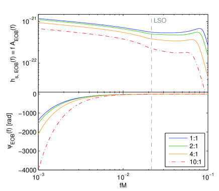
Finally, for the practical purpose of this study, we shall define the complete frequency-domain EOB waveform EOB(f) as the ‘smooth frequency-domain PNEOB hybrid’ constructed in Eq. (IV.3), with the choices and , where is the GW frequency corresponding to the beginning of the longest EOB simulations we generated. More precisely, we have explored a fine grid of mass ratios between and . Given our current implementation and running our simulations on a single desktop computer with a 2.80 GHz quad-core and 4 Gb of RAM, we could, when , start the simulations at , which corresponds to an initial GW frequency . For larger mass ratios, up to , we started at , which corresponds to . The effective amplitude and phase of this complete EOB(f) waveform is represented in Fig. 3 for the values of the mass ratio. Note that this represents simulating , , and orbital cycles, respectively, that took between and minutes of computational time on a single CPU.
The starting point of these simulations is in the very deep inspiral phase of the evolution, where both SPA and PN approximations are perfectly valid. Thus, we shall consider these waveforms as the “correct” ones, using them as the target when computing the inaccuracy of PN-SPA.
V Accuracy upper limit on the junction frequency of hybrid PN waveforms
In this section we shall address a question that is a side-issue with respect to the main aim of this paper, but which is important in the general context of constructing accurate, frequency-domain waveform models. This question concerns the upper limit on the frequency parametrizing999For simplicity and concreteness, we shall henceforth use, for the smooth joining of PN(f) with EOB(f), Eq. (IV.3), a frequency interval with a fixed ratio . This leaves the single parameter to characterize the ‘junction frequency’ between the two waveforms. the joining between a lower-frequency PN(f) waveform to a higher-frequency EOB(f) waveform which does not lead to an undue loss of accuracy for the resulting hybrid waveform PN(f)EOB(f). We shall measure the loss of accuracy of the (frequency-domain) hybrid PN(f)EOB(f) by means of the ‘inaccuracy functional’ , Eq. (29), where denotes the hybrid PN(f)EOB(f), and where denotes our best approximation to the full, exact EOB(f) waveform, i.e., as explained above, the hybrid PN(f)EOB(f) generated with the very low frequency at which we started the EOB simulation. We recall that corresponds to such a non-relativistic and adiabatic part of the inspiral (thousands of orbital cycles before the merger of the BBH) that we can safely consider the lower-frequency PN(f) piece in the hybrid PN(f)EOB(f) as being indistinguishable from the low-frequency part of the exact EOB(f). On the other hand, in view of Fig. 2, we expect that PN(f) will start to significantly deviate from EOB(f) for frequencies somewhere between and , thereby leading to an increasing inaccuracy of the hybrid PN(f)EOB(f) as reaches such values.
There are two motivations for this study. First, though we have been able, for this work, to easily generate many, very long time-domain EOB waveforms, containing thousands of orbital cycles, and then use an automated version of the procedure explained above to generate the corresponding frequency-domain EOB waveforms, it might be useful, when one will need to construct dense banks of accurate frequency-domain EOB waveforms, to cut down to a strict minimum the integration time of each EOB simulation. Determining the maximum leading to some given inaccuracy will be useful in allowing one to start the EOB simulation at a higher GW frequency . A second motivation, is that our result will clearly also tell us the maximum frequency at which we must start a NR simulation (i.e. the minimum number of inspiral orbital cycles it must include) if we wish to be able to extend (to lower frequencies) its Fourier-transformed GW signal by using a simple closed-form PN(f) waveform.
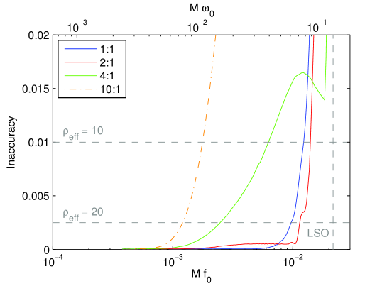
As said above, in order to study the frequency upper limit for the accuracy of PN(f) waveforms, we generate frequency-domain hybrid waveforms , and compute the relative inaccuracy as a function of the joining frequency , or, equivalently, . The inaccuracy functional will also depend on the particular symmetric mass ratio one is considering, and on the value of the total mass (in seconds), since the detector noise curve that enters the definition Eq. (29) depends on the physical frequency (in Hz) and not on the dimensionless scaled frequency . In particular, we shall consider four different values of corresponding to the mass ratios and we shall maximize , for each value of , and , over , i.e. we shall consider the worst case scenario for the loss of accuracy. Since we are considering ground-based detectors, the mass range will be considered to be . This yields, for each value of , the worst-case inaccuracy as a function of . We have done this study for the three different detector noise curves discussed above, and represented in Fig. 1: initial LIGO, advanced LIGO, and advanced Virgo. Note that the inaccuracy functional only depends on the shape of these noise curves, and not on their absolute magnitudes.
We represent in Fig. 4 the inaccuracy, , maximized over , as a function of the junction frequency , for different mass ratios, and for the Advanced LIGO noise PSD. According to Eq. (30), the maximum inaccuracy that we can tolerate depends both on the signal-to-noise ratio, , and on the choice of an additional “safety factor” . More precisely, what matters is only what we can call the effective SNR, namely . Two models will be indistinguishable if their relative inaccuracy is smaller than . In the present section we shall consider the effective SNRs or . Note that, as we expect typical observations to have a real SNR of , the inaccuracy limit with corresponds to taking , i.e. to allowing the inaccuracy of the model waveform to double the effect of the detector noise. It would seem more reasonable to take at least , i.e. to consider an effective SNR of .
The most interesting feature of Fig. 4 is the notable difference between the case of mass ratios near unity (namely and ), and the case of large mass ratios: and . When Fig. 4 shows that the accuracy loss remains quite small up to frequencies rather close to the Schwarzschild-like LSO frequency . [One should, however, recall that the real (EOB-predicted) LSO frequency is larger, being close to .] In other words, the PN(f) model produces accurate waveforms up to near the LSO when . By contrast, when the mass ratio increases, namely , the inaccuracy gets significant for frequencies which are much smaller than the LSO frequency (especially if one considers the threshold ). As the number of orbital cycles between and is approximatively given by the “Newtonian” estimate (see, e.g. , DIS:2000 )
| (46) |
such a smaller means a much larger number of orbital cycles left between and, say, (both because of the power-law dependence on , and of the explicit proportionality to ). Even if we consider the somewhat lax threshold , we see on Fig. 4 that the PN(f) waveform can be used: up to when or ; only up to a twice smaller frequency when ; and only up to a seven times smaller frequency when .
The Table of Fig. 4 gives more quantitative information about this accuracy upper limit on the junction frequency to PN(f). The table considers all three detectors noise PSD, and the two thresholds and (the quantitative data pertaining to the threshold are given within parentheses). In particular, the last two columns indicate the conversion of in separation between the BHs, and in number of orbital cycles left before reaching the merger. [The conversion between and was formally done using the approximate formula , while the number of orbital cycles was computed by using the underlying EOB dynamics; defining the “merger” as the instant where the (metric) waveform reaches its maximum amplitude.]
Notice the steep rise of the number of orbital cycles left as the mass ratio gets larger than 4. For a given accuracy threshold the Advanced Virgo detector is the most demanding one for the PN(f) model because the shape of its effective noise curve peaks at a lower frequency, but note that, for a given signal amplitude the SNR of Advanced Virgo would be smaller than that of Advanced LIGO.
Leaving to future work DNT2 a detailed discussion of the precise meaning of these results (notably in terms of the intrinsic accuracy of the PN(f) waveform), let us mention that our results suggest that the “inaccuracy” of a frequency-domain hybrid, say PN(f)NR(f), between a lower-frequency PN(f) and a higher-frequency NR(f) waveform will be similar to the one plotted in Fig. 4. In particular, we think that, if one requires the same type of threshold on the inaccuracy, the number of orbital cycles before merger will have to be similar to the numbers indicated in the last columns of the Table. On the other hand, let us recall that numerical simulations are computationally very expensive, and the current longest waveforms being produced span at most the last orbital cycles of the evolution Hannam:2009rd ; Hinder:2010vn . Recently, a joint effort between several NR groups and scientists producing analytical models NRAR_col has begun to make use of TeraGrid resources in order to produce longer and more accurate simulations. However, one does not currently foresee the possibility of producing more than orbital cycles. Comparing these current NR capabilities with the numbers we are obtaining here for the upper-frequency-limit of frequency-domain hybrids using PN(f) for , we observe that, for mass ratios it will be impossible to “join” a PN(f) waveform to a NR(f) one without incurring an unacceptably large accuracy loss. In intuitive terms, one can say that we are here facing the probable existence of a frequency gap where neither PN theory nor current NR simulations are able to provide accurate enough information. We think, however, that the effective-one-body approach, aided by suitably designed NR calibrations, may be able to bridge this dangerous frequency gap, and then to construct some accurate-enough complete waveform models.
|
Initial LIGO ; () orbits pre-merger 1:1 () () 2:1 () () 4:1 () () 10:1 () () Adv. LIGO ; () orbits pre-merger 1:1 () () 2:1 () () 4:1 () () 10:1 () () Adv. Virgo ; () orbits pre-merger 1:1 () () 2:1 () () 4:1 () () 10:1 () () |
VI Validity ranges of PN and of Phenomenological models
This section will present the central results of our work: namely the quantitative study of the ineffectualness and of the inaccuracy of the closed-form, frequency-domain waveforms presented above, with respect to the fiducial target waveform defined by the NR-calibrated EOB waveform (computed in the frequency-domain, as explained above). [For brevity, we shall sometimes denote the NR-calibrated EOB waveform as EOBNR.] Our aim is to assess the regions of the parameter space of (non-spinning) BBHs, i.e. and , where:
-
•
either one of the closed-form models (PN(f), PhenV1 or PhenV2) provides an effectual representation of EOBNR; as measured by the value of the effectualness, see Eq. (19); or,
-
•
either one of the closed-form models (PN(f), PhenV1 or PhenV2) provides an accurate representation of EOBNR; as measured by the value of the inaccuracy, see Eq. (30).
We did not investigate whether a suitable PN(f)PhenV2(f) hybrid might be closer to EOBNR(f). Indeed, Phen waveforms are already supposed to have incorporated a PN-type early behavior, with an NR-type later waveform.
Before presenting our quantitative results, let us anticipate some general aspects of our results by noting that one a priori expects that neither PN(f) nor phenomenological models will be able to accurately describe all stages of the evolution of BBHs. Through the detector noise PSD, this lack of uniform physical validity will then translate into validity ranges in the space of physical parameters, and . In particular, we expect the PN(f) waveforms to only provide a valid description of the early inspiral stage of the evolution up to a certain frequency [, see Sec. V above], but to start failing as the two BHs get close and the dynamics becomes more relativistic and less adiabatic. Given the inversely proportional relation between the total mass and the frequency, inspiral-only models, such as PN(f) (or, for that matter, any other PN waveform), will be adequate only for searches of relatively low mass systems, , in initial ground-based detectors (for such systems the merger occurs at higher frequencies than the detectors sensitivity window; see the horizontal segments near the bottom of Fig. 2). On the other hand, the phenomenological models are built to effectively describe the merger phase of the evolution. They can therefore be expected to provide an adequate method to search for high mass systems (say ), where the merger phase is the main contribution to the SNR (see Fig. 2). This preliminary discussion suggests that there might exist an intermediate range of masses, around , where none of the closed-form models can provide an accurate description. We shall see that this is indeed the case.
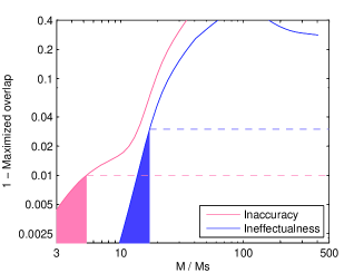
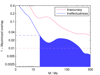
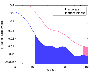
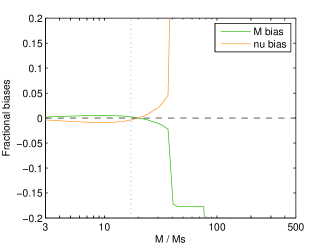
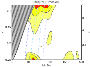
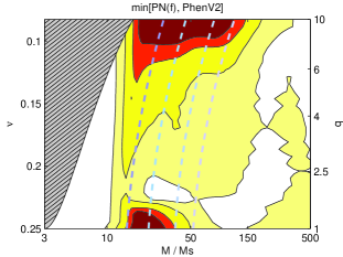
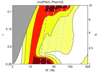
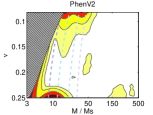
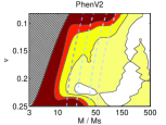
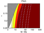
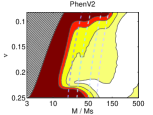
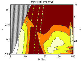
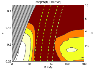
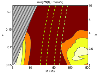
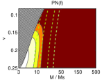
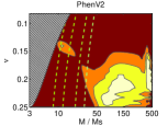
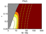
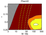
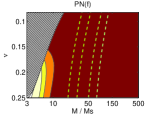
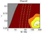
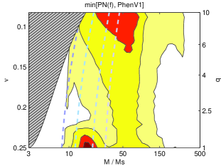
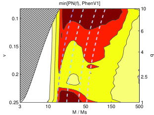
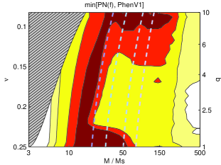
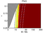
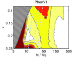
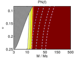
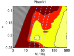
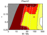
Our quantitative results on the validity range of these two models, both from the effectualness (detection) and accuracy (measurement) points of view (using EOBNR waveforms as fiducial targets), are presented in Figs. 5 and 6, and in Table 1. We now explain them in detail.
 |
 |
 |
 |
 |
 |
| (a) PN | (b) PhenV1 | (c) PhenV2 |
|
Initial LIGO
1:1
2:1
4:1
10:1
Adv. LIGO 1:1 2:1 4:1 10:1 Adv. Virgo 1:1 2:1 4:1 10:1 |
Initial LIGO
1:1
2:1
4:1
10:1
Adv. LIGO 1:1 2:1 4:1 10:1 Adv. Virgo 1:1 2:1 4:1 10:1 |
| (a) ineffectualness | (b) inaccuracy |
| PN(f) – PhenV2 | ||||||
| : |  |
 |
 |
|||
|---|---|---|---|---|---|---|
 |
 |
 |
 |
 |
 |
|
| : |  |
 |
 |
|||
 |
 |
 |
 |
 |
 |
|
| (a) iLIGO | (b) aLIGO | (c) aVirgo | ||||
| PN(f) – PhenV1 | ||||||
| : |  |
 |
 |
|||
|---|---|---|---|---|---|---|
 |
 |
 |
 |
 |
 |
|
| (a) iLIGO | (b) aLIGO | (c) aVirgo | ||||
VI.1 Effectualness. Detection
As recalled above, when one is only interested in detecting GW signals from compact coalescing objects but not in the extraction of accurate physical parameters from the observations, an important indicator to evaluate a given approximated model is the effectualness, , Eq. (14), which represents the fractional loss of SNR entailed by the use of a sub-optimal match filter. Actually, the most important indicator is the “effective effectualness” which takes into account the discrete character of the template bank (see above). We have indicated in Eq. (19) the range of thresholds that one usually considers for the effectualness. Let us say again that the often quoted effectualness level of (corresponding to an ineffectualness ) is a very minimal requirement that does not seriously take into account the constraints coming from the discrete nature of the template bank. It would seem more appropriate to require an ineffectualness near , which, combined with an equivalent minimal match , guarantees that one does not lose more than of the potential events.
To have a first view of the influence of choosing an effectualness (and accuracy) threshold on the validity range of various models, the top panels of Fig. 5 plot as dark gray (blue online) lines the ineffectualness as a function of the total mass, for a fixed mass ratio of 4:1, and using the Adv. LIGO noise PSD. The three top panels respectively correspond to the three closed-form models introduced above: PN(f), PhenV1 and PhenV2. [We recall that EOBNR is used as fiducial “exact” target .]
These top panels show that as one imposes a stricter threshold on the effectualness (i.e. a smaller level for the ineffectualness ) the validity range of the various models change in the direction expected from the preliminary discussion above. For the PN(f) model (left top panel), the validity range at some ineffectualness threshold is an interval of the type , where the maximum allowed total mass decreases as one decreases . For instance, at the level , indicated by the upper dashed line in the left top panel (blue online), one has , while the stricter level leads to . This behavior is consistent with the fact that the PN model is only adequate during the inspiral, up to some maximum dimensionless frequency (see Fig. 4). Then, given the fixed detector sensitivity window in Hz, this translates into an upper limit on the total mass: . On the other hand, the phenomenological models considered in this paper were built with the specific aim of reproducing the late inspiral, merger and ringdown phases of the evolution found by NR simulations, and therefore, they should be most effectual for the detection of high mass systems. And, indeed, one finds that, for the phenomenological models (right top panels) the validity range at some ineffectualness threshold is an interval of the type , where the minimum allowed total mass increases as one decreases . For instance, at the level , and for PhenV2, as indicated by the upper dashed line in the rightmost top panel (blue online), one has , while the stricter level leads to a much larger value: . [For PhenV1, these minimum masses are for ; and for ]. This example (with and Adv. LIGO) shows that: (i) at the minimal effectualness level there is an overlap between the ‘low-mass’ interval where PN(f) is effectual, and the ‘high-mass’ interval where PhenV2 is effectual, so that the union of the two template banks is able to detect the full mass range; while, by constrast, (ii) at the stricter effectualness level , there exists a mass gap, between and , in which neither PN(f) nor PhenV2 (nor Phen V1) is effectual enough. We shall focus on these mass gaps below, after having commented upon the other panels of Fig. 5.
The bottom panels of Fig. 5 complete the discussion of the effectualness calculation by showing the fractional biases between the actual and parameters and the ones that maximize the overlap between the model and the target waveforms in the maximization, Eq. (15). In our analysis, we have restricted the parameters to have a physical meaning, i.e. . However, the results obtained by allowing the parameters to be unphysical remain almost the same: only a small improvement of the effectualness near the equal-mass region is observed, because this is where the restriction becomes relevant. By looking at our particular results in Fig. 5 for and the Adv. LIGO noise PSD, we observe that the systematic biases in estimating the parameters are smaller than for when using PN waveforms; while they are smaller than for ( for ) for when using phenomenological models. Anyway, these fractional biases are merely informative since one would have to compare them with typical statistical errors from a proper parameter estimation study in order to truly interpret the consequences of having an effectual, but not accurate, model. Let us mention that several works in the literature have studied the parameter estimation of BBH coalescences with ground-based detectors, using either PN templates Cutler:1994ys ; Poisson:1995ef ; Sintes:2000 ; AISS_2005 ; VanDenBroeck:2006ar ; Rover:2006bb ; vanderSluys:2008qx ; Veitch:2009hd or phenomenological ones Ajith:2009fz .
Let us now study in detail the mass gaps where none of the closed-form models are effectual enough. Since the non-precessing phenomenological waveforms (PhenV2) PhenV2 are always more accurate and produce smaller mismatches with EOB than the original non-spinning ones (PhenV1) PhenV1 , we shall study, for various effectualness levels, the region of parameter space where the union of PN(f) and PhenV2 models fails to be effectual. As we saw above, this region is defined, for each given ineffectualness level , and for each given value of , by the mass gap between and , i.e. by the interval , when it is non empty. These mass gaps are listed in Table I(a) as three sub-tables for the different detectors: initial LIGO, advanced LIGO and advanced Virgo; and in there the intervals are given for four different mass ratios () and for four different effectualness levels: .
In Table I(a), one can observe how these “ineffectualness intervals” become wider as we go to more restrictive effectualness bounds, and also as we consider more sensitive detectors. Concerning their dependence upon , we see that mass ratios between 2:1 and 4:1 generally lead to the narrowest intervals, while the other mass ratios (especially ) lead to wider intervals, mainly because of the increase of their right end: . Typically, the lack of effectualness of the closed-form models takes place for intermediate mass systems, from a total mass of to , depending of the mass ratio. For instance, considering the Adv. Virgo noise PSD and allowing a maximum loss of SNR of , the analytical models would not be valid to search for equal-mass systems between and ; for 2:1 systems from to ; for 4:1 from to and for the most extreme mass ratio 10:1 from to .
Finally, in order to have a better view of the regions of the parameter space where the union of PN(f) and PhenV2 fails to be “-effectual” (i.e. where the infimum of the ineffectualnesses of PN(f) and PhenV2 is larger than ), we have determined the ineffectualness intervals on a finer grid resolution in the whole parameter space. The contour plots in the large top panels of Fig. 6 and Fig. 7 represent the result of this ineffectualness calculation when one considers the two closed-form models simultaneously. By contrast, the small sub-panels located below the large upper panels represent the separate values of the effectualnesses of the two closed-form models: PN(f) on the left and PhenV2 on the right. The four contour lines represent the same effectualness thresholds used in Table 1 (i.e. ), but the higher resolution in allows us now to observe the continuous evolution of the validity ranges as the mass ratio varies. As before, normally the left-most bounds are determined by the total mass values above which the PN(f) model is not valid anymore, whereas the right-most limits are given by the minimum mass values where phenomenological models are effectual. Choosing a certain ineffectualness level , the corresponding regions (from the darkest one in which to the lightest [but not white] one where ) on the contour plots represent the domain of parameter space where none of these closed-form models could be used in an actual search, even for the mere purpose of detection, without requesting a faithful recovery of the physical parameters. Let us start by noting that, in the case of initial LIGO, the simultaneous use of PN and PhenV2 waveforms (i.e. , in fact, the use, for each particular of the best of the two, namely the one having the smallest ineffectualness for these values of and ) allows one to cover the full parameter space with an ineffectualness , i.e. an effectualness larger than . At higher effectualness levels, like or , one is progressively losing the complete coverage of the parameter space. It is, however, interesting to see, on the smaller sub-panels below the top left panel, the separate performances of PN and PhenV2 waveforms: PN has a good effectualness only in the small-mass corner on the left. On the other hand, PhenV2 (for initial detectors) is effectual in a large part of parameter space, though it fails to be effectual in three sub-zones: (1) in the small-mass corner, (2) in an “island” centered around , , and (3) in another island located above . This good effectualness performance of the closed-form models is, however, drastically decreased in the case of advanced detectors. Note, for instance, how, in the case of advanced LIGO, the PhenV2 waveform fails to be effectual in an extended “C-shaped” region which covers many physically interesting systems: notably the range , a domain located in the high q region, as well as essentially all systems with . However, the simultaneous use of PN and PhenV2 waveforms allows one to substantially reduce the extension of this ineffectualness domain. As seen on the middle top panel, the union of the two waveforms fails to be effectual only in two “islands” located either around , or around . Note also, how, in the case of the advanced Virgo detector, requiring an ineffectualness (i.e. an effectualness ) excludes the joint use of closed-form waveforms in an extended “ridge” which separates a low-mass region on its left from a high-mass region on its right.
Before discussing the “inaccuracy analogs” of the ineffectualness regions plotted in the top panels of Fig. 6, let us mention the meaning of our results for the most recent LIGO-Virgo searches for low-mass compact binary coalescences (CBC) using PN templates. In particular, CBC_search_1 ; CBC_search_2 ; CBC_search_4 have performed searches for and CBC_search_3 for . Upper limits for the particular systems , and have also been set in CBC_search_2 ; CBC_search_4 . Our results show that the PN templates used in all the searches done so far (with the initial LIGO noise PSD) had an ineffectualness for systems with , and that this performance could be extended to most of the analyzed parameter space by also including phenomenological waveforms. However, in a physically significant part of the parameter space (namely systems with a total mass and mass ratios, either or ), the ineffectualness of the PN templates exceed , and even . Keeping in mind that the discretized template bank used in the searches had a maximal mismatch of , this means that, in a significant part of parameter space, the searches could be missing , i.e. , , or even of the potential events. The probability to miss potential events because of the ineffectualness of closed-form waveform models will become much more significant in searches performed with advanced detectors (see top panels of Fig. 6). This indicates the need to use more effectual templates, and to construct template banks having a smaller maximal mismatch.
VI.2 Accuracy. Measurement
As recalled above, if one wishes to use some waveform model not only for detecting the presence of a GW signal, but also for measuring the physical information contained in the GW signal, one needs this waveform model to satisfy a stricter condition than the one of effectualness studied in the previous section. Namely, the waveform model must be such that its inaccuracy , Eq. (27), is smaller than , where denotes what we called the effective SNR (which is larger than the real SNR by a safety factor ), see Eq. (30). Thus, the accuracy condition for each model shall be well defined after choosing: (i) what is the target signal that one is trying to measure; and (ii) a certain level for the effective SNR, . As before, we shall choose as fiducial target signal the NR-calibrated EOB waveform, EOBNR, whereas the effective SNR levels that we shall consider are . Note beforehand that most of these levels are quite lax, and that only the last one is likely to be a really useful accuracy requirement. [Indeed, we expect typical first observations to have , and, as discussed above, adding a safety factor seems to be a minimal requirement.]
Following the same strategy as in the previous Section, we start by studying how the inaccuracy evolves with the total mass of the system for a particular mass ratio, 4:1, and a particular noise PSD, namely Advanced LIGO’s. The results are plotted as light gray (red online) lines in Fig. 5 for the three closed-form models we have considered (using EOBNR waveforms as target). As expected from our effectualness results (remembering the fact mentioned above that the inaccuracy is a non-minimized version of – twice – the ineffectualness), we find that the PN(f) model is only accurate for low mass systems, while the opposite happens for the phenomenological models. For instance, if we assume an effective SNR of , we obtain that the PN(f) model is only accurate for describing systems lighter than , whereas PhenV1 is not accurate for any system we have analyzed within and PhenV2 only provides an accurate representation for systems heavier than . In this case, we are finding a very wide inaccuracy interval, where neither PN(f), nor any of the phenomenological models provide waveforms accurate enough to extract faithful information from the GW data.
We have determined the inaccuracy intervals of the three analytical models101010As in Sec. VI.1, their left-most boundaries are determined by the PN(f) model and the right-most ones by PhenV2. for different mass ratio cases, using also different detector noise PSDs and setting different SNR levels; the results are summarized in Table 1(b). Comparing the right part of this Table (“inaccuracy”) to its left part (“ineffectualness”) we can see how stricter the accuracy condition is, compared to the effectualness one. Typically we are now finding that PN(f) waveforms are only accurate up to a few ’s, leaving then a wide gap of at least until phenomenological models provide an accurate representation of the observed waveform. Note in particular that we find in nearly all cases that the expected paradigmatic BBHs with cannot be accurately described by any of the closed-form waveforms. In other words, we find that, in a large fraction of the parameter space, no Fourier-domain closed-form models can be used for measurement purposes.
In order to better visualize the inaccuracy gaps that we are finding in parameter space, we represent in Fig. 6 (bottom panels) the contour plots corresponding to the inaccuracy levels used in Table 1, namely , corresponding to . This means that the darkest zone is the region where the inaccuracy111111Note that we plot as inaccuracy domains at some level the region of parameter space where both PN(f) and PhenV2 have an inaccuracy larger than . is larger than , the next, less dark, zone is the region where (but ), etc., until the lightest [but non white] zone where (but ). Note how the darkest zones in the bottom figures, where the inaccuracy is larger than the very lax level , span (even for initial detectors!) a very wide region of parameter space. For advanced detectors, this region of “large inaccuracy” can be schematized as: (i) if , all the systems with belong to this large-inaccuracy zone, while (ii) if , all systems, whatever be their mass, belong to this large-inaccuracy zone121212Let us recall that phenomenological models were created using NR data only for .!
The main conclusion of this study is that closed-form models can be used, for measurement purposes, only in two small islands of parameter space: (i) the vertically elongated white islands on the left of the bottom figures, corresponding to small-mass systems (say with ), where PN(f) gives an accurate waveform; and (ii) the small whitish islands on the right of the bottom figures, corresponding to some special, large-mass systems (with and ), which can be accurately described by PhenV2(f). In most of the rest of parameter space, the inaccuracy of the closed-form models is larger than the minimal level required for extracting faithful physical information from the GW observations.
VI.3 Implications of the non-validity regions
Let us consider in more detail the meaning and implications of the presence of extended regions in parameter space where closed-form models are either ineffectual or inaccurate (dark, and darkish, regions in Figs. 6 and 7).
To have a better grasp of the physics involved in the systems behind the abstract parameter-space representation, we have overprinted on Figs. 6 and 7 four dashed lines which gauge the number of orbital cycles (before merger) contributing of the SNR. [The consideration of a fraction of the SNR of order is natural in our discussion where we are ultimately interested in effectualnesses of that order or better.] We recall that the SNR2 is given by the logarithmic frequency integral of the squared ratio between the (dimensionless) effective GW signal amplitude and the (dimensionless) effective GW noise . The integrand is maximum at some frequency and decreases on both sides of . For each given detector, each given fraction of SNR (say ), and each given BBH system, we can then find two frequencies, say , with , and such that . Then, we can count the number of orbital cycles, say , (defined by the underlying EOB dynamics) spent by the considered BBH system between the GW frequencies and . [When is reached after the merger, one counts the orbital cycles between and merger.] Actually, the choice of the two frequencies is not unique as we can move and so as to keep the integral fixed. But we (numerically) looked for the values of and that minimize the number of orbital cycles spent between them. The result is unique, and defines a number of orbital cycles which is a function of the parameters of the system (i.e. , in our case, of and ) and of the choice of detector noise curve. [In most cases, is dominated by the number of orbital cycles spent in the inspiral, and is approximately given by the first term (with ) of the Newtonian estimate Eq. (46), namely . But this formula does not help to know the precise value of because the value of the minimizing lower frequency is itself a function of and the detector PSD, which depends very much on the relative location of the peak of the detector sensitivity curve , and the merger.] Going from left to right, the four dashed lines in Figs. 6 and 7 represent the locus of the systems for which is constant, and successively takes the values . Clearly, for a given , will increase as the total mass decreases. This means in particular that any system lying on the left of the left-most dashed line will have , and similarly for the other lines.
One should view the level lines as a (partial) “intrinsic coordinate system” in parameter space. That is to say: a level line has a more direct meaning, from the data analysis point of view, than a coordinate line These lines allows one also to make a connection with the capabilities of NR simulations. Indeed, the current longest NR simulations have at most orbital cycles before merger. Anticipating faster NR simulations, we can hope that they will be able to explore in the foreseeable future orbital cycles, and possibly . On the other hand, it will probably be very difficult for NR to simulate orbital cycles. We shall discuss below the issue of the minimum number of orbital cycles from NR simulations which would be needed to inform us, in the most effective way, about the dynamics and radiation of BBHs.
Having in mind the significance of the dashed lines in the figures, we can use them to highlight some interesting physical facts that appear on the inaccuracy plots, i.e. the lower plots of Fig. 6. Let us first note that these plots exhibit the existence of two “islands of accuracy” (i.e. whitish zones), within an “ocean” of inacceptably large inaccuracy (darker zones). [For definiteness, we shall define this ocean of inaccuracy as the union of the two darkest zones.] The (vertically elongated) island on the left of each plot lies in the small-mass region and corresponds to BBH systems for which the inspiral PN(f) waveform provides, by itself, an accurate description of the full EOBNR waveform. The other whitish island on the right of each plot (roughly centered around , ) corresponds to BBH systems for which the PhenV2(f) waveform accurately agrees with the EOBNR waveform.
-
•
The first fact is that the left islands of accuracy (which we can call the islands of accuracy of pure PN waveforms) possess as right boundaries (i.e. their “shores” in the dark ocean of inaccuracy) some lines which are approximately parallel to the dashed, lines, with large values of the constant. For instance, for initial LIGO, the right boundary of the left (PN) island is approximately located along the , while for advanced LIGO it is approximately along the line. For advanced Virgo the value of on the boundary is significantly larger than .
-
•
The second fact, is that the right islands of accuracy (i.e. the islands of accuracy of phenomenological waveforms) do not extend, on their left side, beyond lines, with a rather small value of the constant, say or so. Notice also that the accuracy zone of the phenomenological waveforms seems to be restricted to . This probably reflects the fact that the construction of phenomenological models did not correctly incorporate the known PN inspiral phasing, and it is consistent with the parameter range of NR waveforms used to build these models PhenV1 ; PhenV2 .
The first fact is easily understood. Indeed, the PN(f) model does not include any merger signal. Therefore it can have a small inaccuracy with respect to the target signal (which include the merger) only for systems whose SNR is nearly completely given by the inspiral signal. The second fact is a priori more surprising, because the motivation for the construction of phenomenological signals was to approximately describe a waveform comprising all the needed components of the full signal, namely a PN-type inspiral, a NR-described merger, and a leading quasi-normal-mode-type ring-down. However, we can see in Fig. 2 that the Phen waveforms exhibit significant disagreements, both in amplitude and in phase, with the target (EOBNR) signal. More quantitatively, if we remember, from the discussion in the Sec. IID above, that an inaccuracy smaller than implies that the noise-weighted quadratic sum of the fractional amplitude, and phase, differences must be smaller than , we understand upon looking carefully at Fig. 2 that the Phen models are too coarse approximations to be accurate during most evolutions that will have a significant mixture of inspiral and merger. The conclusions we can draw from these remarks will be discussed in the next section.
The lack of validity of these analytical models in certain regions of the parameter space, will require the use of more accurate (and also more time consuming) models when performing a search, such as, either full NR simulations, or a new and more complex phenomenological model, or EOB waveforms. In particular, the limited accuracy of PN(f) that we are observing, specially at more extreme mass ratios, will require filling a large gap of the BBH evolution between where PN-SPA fails and the merger (it may represent several hundreds of orbital cycles, as we have seen in Sec. V), that will probably be computationally unachievable for full NR simulations, but much more reasonable for semi-analytical methods such as the EOB approach.
VII Conclusions
Our knowledge of the dynamics of coalescing BBH systems and their gravitational emission has experienced a huge progress during the last years, both with the improvement of analytical methods, namely PN expansions and EOB approaches, and the breakthroughs that occurred in NR. A crucial question at this stage is to know whether the recently accumulated PN+EOB+NR knowledge is sufficient for the GW data analysis needs of the present and upcoming GW detectors. We can classify the currently available model waveforms into several categories:
-
•
closed-form, frequency-domain models which are only accurate in a limited range of the evolution, e.g. PN(f), ring-down models and (NR-fitted) phenomenological models (which try to extend their validity range by combining information coming from PN(f), ringdown(f) and some NR simulations);
-
•
EOB models, which cover the whole evolution, and which are defined in the time-domain by integrating ODEs; they can easily incorporate information coming either from PN and from NR;
-
•
full NR simulations, which are necessary for describing the nonperturbative physics around merger, but can only cover a limited number of orbital cycles () because they are very time consuming in terms of computational costs;
-
•
time-domain PN models (either using closed-form expressions or integrating ODEs), which are limited to the inspiral part of the evolution;
-
•
various types of hybrid models, joining together (either in the time-domain, or in the frequency-domain) early PN-type waveforms to later NR waveforms, so as to cover the whole evolution.
The time needed to generate a waveform in one of these categories varies by many orders of magnitude between, say, a closed-form frequency-domain waveform (a fraction of a second on a single CPU); an EOB waveform (several seconds, also, on a single CPU); or, a full NR simulation ( a month on a computer cluster with several hundreds of CPUs). From the data analysis point of view, it would be quite useful to be able to generate waveforms as fast as possible [actually, the real issue is to be able to access a dense bank of them very fast]. Though some trade off between speed and accuracy can be allowed for, there are minimal accuracy requirements that waveforms have to satisfy. This is why our present paper has focused on a detailed analysis of the accuracy of the fastest existing waveforms, namely the closed-form, frequency-domain ones.
In this paper, we have performed an extensive study, in the whole parameter space, of the validity of the closed-form, frequency-domain models (for non-spinning BBHs): i.e. PN(f) and phenomenological models. We have studied both their effectualness (detection) and their accuracy (measurement) using as target model the currently most accurate NR-calibrated EOB waveform. We have considered both initial GW detectors and advanced ones.
Our conclusions concerning closed-form, frequency-domain waveform models are:
-
•
When considering initial interferometers, these closed-form models are just effectual enough to be used for detection. Though their effectualness (14) is, indeed, larger than in nearly all the parameter space131313Apart from a small island near and in the PhenV1 plot, Fig. 7, it is smaller than in two separate islands in parameter space, and smaller than in sizable regions of parameter space. See lef–top panel of Fig. 6 and left panel of Fig. 7. In particular, notice (on the smaller sub-panels) that most of the effectualness is provided by the phenomenological model, except for the very low mass end, and also around the crucial , region where PhenV2 fails to be effectual.
-
•
When considering initial interferometers, they are not accurate enough to be used for measurement. Their inaccuracy, Eq. (27), is, indeed, larger than the threshold corresponding to an effective SNR of (which is an very low threshold) in a huge domain of parameter space. See left–bottom panel of Fig. 6 where the darkest zone is the region where the inaccuracy is larger than . The union of the darkest and second darkest zone correspond to an inaccuracy larger than , which is still a very low threshold.
-
•
When considering advanced interferometers, they are neither effectual, nor accurate in large domains of parameter space. More precisely, the domains of ineffectualness are the extended islands given by the dark zones of the two right, upper panels in Fig. 6 (the darkest zone failing to be effectual, and the second darkest one failing to be effectual). Concerning the domains of inaccuracy they have become so prominent and extended in the two right, lower panels in Fig. 6 (with respect to the domains of ineffectualness in the plots above them)141414In other words, we can say that the (dark) islands of ineffectualness of the upper panels have “percolated” among themselves, and left only a reverse landscape where the accuracy zones exist only as separate islands. that it is better to visualize them as an ocean of inaccuracy containing only two well-separated islands of accuracy (namely the whitish zones in the two right, bottom panels). In the left island of accuracy, PN(f) provides an accurate model for small-mass systems, while, in the right island of accuracy, PhenV2 provides an accurate model for systems with total mass , and mass ratio .
Our conclusion is therefore that the current, existing closed-form, frequency-domain models fail to be accurate enough to be used for measurement purposes, even with initial GW detectors. On the other hand, if one uses jointly the two closed-form models with initial GW detectors sensitivities, they provide a -effectual coverage of the full parameter space, and a -effectual one in an important fraction of parameter space. These effectualness levels are significantly reduced when considering advanced detectors noise PSDs or taking the waveform models separately. These results call for the development of more accurate versions of these phenomenological models. In particular, we think that an important defect of the V1 and V2 versions of the phenomenological models is that they do not correctly incorporate the analytically known (PN) phasing behavior during the (early) inspiral. One can indeed see on Fig. 2 how this leads to large dephasings during the inspiraling phase. In turn, these dephasings cause the ineffectualness and inaccuracy properties. [See, below, additional results concerning the recently constructed V3 version of the phenomenological models.]
In terms of the (partial) intrinsic coordinate system defined by the level lines , we can summarize the performance of PhenV2 model saying that it can provide an accurate representation of the last orbital cycles before merger for systems, and an effectual representation of signals with no more than visible orbital cycles within the mass ratio range . [PhenV1 model is not accurate enough anywhere and its effectualness is restricted to signals with visible orbital cycles in the same mass ratio range as PhenV2]. Of course, as we consider more sensitive detectors, these upper limits on translate into a restriction of a larger portion of the parameter space.
Also, a side result of our study is the determination of the maximum frequency, as as function of the mass ratio, at which PN(f) waveforms can be ‘joined’ onto EOBNR (in the frequency domain) without undue loss of accuracy. Our results are summarized in Fig. 4 and show wide validity ranges for PN(f) up to less than orbits before merger for 1:1 and 2:1 systems, but much more worrying results when considering systems. In particular, we find gaps of orbital cycles for [ orbital cycles for ] between the low-end of the PN(f) validity range and the merger; which can hardly be covered with (computationally intensive) NR simulations.
We are fully aware that the analysis that led us to all these conclusions depends on our use of the EOBNR waveform as a reference model for defining the inaccuracy functional Eq. (27), Eq. (29). Strictly speaking the dark zones in Fig. 6 only represent the regions of parameter space where the fractional squared Wiener distance between the closed-form models and EOBNR is larger than . However, we think that there is a good rationale for considering that our results tell us something about the exact inaccuracy of the closed-form models, i.e. their fractional squared Wiener distance away from the (unknown) exact waveform. Indeed, one should keep in mind that the inaccuracy level corresponding to the two darkest zones corresponds to fractional amplitude, and phase inaccuracies (in radians), which are only . By comparison, the NR-calibrated version of the EOB formalism that we used here Damour:2009kr has been proven to agree with some of the current most accurate NR simulations with significantly smaller amplitude and phase inaccuracies. More precisely, in the case, the phase disagreement between EOB and the Caltech-Cornell data Boyle:2007ft ; Scheel:2008rj remained smaller than radians during the entire orbital cycles of inspiral and plunge, which is comparable with the estimated NR errors. At the merger and during the ringdown took somewhat larger values ( radians), but it oscillated around zero so that, on average, it stayed very well in phase with the NR waveform. As for the fractional amplitude disagreement it remained smaller than about during the entire inspiral, and only momentarily exhibited a larger value () just after the merger. In the and cases, the agreement between EOB and the Jena data (published in Damour:2008te ) was excellent, and within the numerical errors during the entire span of the simulation (which comprised GW cycles); see Fig. 10 in Damour:2009kr . However, the numerical errors in the latter case were significantly larger than in the case, but smaller than the level used in our inaccuracy study (remaining probably smaller than radians). Let us also mention that an earlier version of the EOB formalism has also been succesfully calibrated (within NR errors) to accurate NR simulations for several mass ratios and Buonanno:2009qa (however, the -orbit simulations used in Buonanno:2009qa cover only part of the late inspiral, without the merger). For , no EOB–NR calibrations have been published yet, due to lack of accurate and long enough NR waveforms available to us in this mass-ratio regime; however, let us note that recent work Bernuzzi:2010ty ; BN2010b has accurately confirmed the validity of the EOB waveform model in the extreme mass ratio limit.
We have also explored how the results would change in the hypothetical case where the low frequency cut-off of the advanced detectors would be increased from to , since improving the low frequency region of the ground-based detectors sensitivity is always the most challenging task from the experimental point of view. All our results remain almost unaltered, except for a tiny improvement in the effectualness of phenomenological models due to a reduction of the number of visible orbital cycles. In any case, all the conclusions described in this article would remain the same.
| PhenV3 | |||
| : | 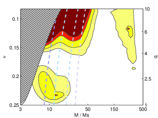 |
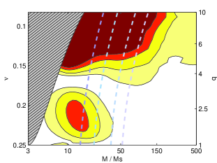 |
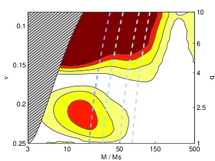 |
|---|---|---|---|
| : | 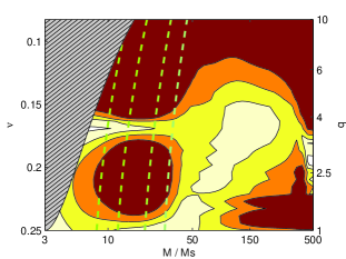 |
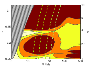 |
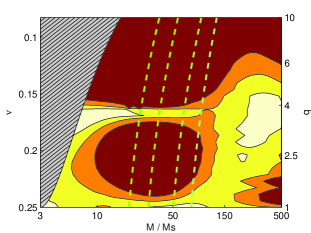 |
| (a) iLIGO | (b) aLIGO | (c) aVirgo |
By the time this article was ready for submission, a new phenomenological waveform model for non-precessing spinning BBH systems was published by Santamaria et al. Santamaria:2010yb . This model (that we shall call “PhenV3”) represents an improvement over the previous PhenV2 model. This new PhenV3 model aims at describing the whole BBH coalescing process by joining a state-of-the-art PN description of the early inspiral (which was lacking in V1 and V2) to separate phenomenological representations of a “pre-merger signal”, and a “ring-down” one. In view of the improved nature of this PhenV3 model, we have decided to complete our analysis by studying its effectualness and accuracy performances (i.e. the analogs of Figs. 6 and 7 above). Our results for the PhenV3 waveform151515The authors of Santamaria:2010yb kindly let us know about the existence of a typo in their Eq. (5.12): the ‘’ parameter of the Lorentzian function should read instead of . Here, we have used the corrected expression when generating our results. are displayed in Fig. 8. As this new model now incorporates a 3.5 PN-accurate description of the early inspiral, we directly plot in Fig. 8 the ineffectualness and inaccuracy (with respect to EOBNR) of PhenV3(f) alone, without computing the infimum with respect to PN(f). If we focus our attention on the region (where the phenomenological parameters were fitted), we observe that the PhenV3 model is effectual for initial detectors and effectual when considering advanced detectors noise PSDs. The effectualness is higher for massive systems, , (where only the last few cycles of the evolution are observable) and reaches minimum values in the [astrophysically relevant] region around (where there are still many observable cycles but PN theory has already started to fail). Notice that these results are consistent with the overlaps plotted in Fig. 10 of Santamaria:2010yb , despite the fact that here we do not maximize the effectualness over any spin parameter, as we have restricted ourselves to non-spinning systems. The fact that the ineffectualness (as well as the inaccuracy) is maximum around and , is compatible with the fact that, when plotting the analog of Fig. 2 for the PhenV3/EOB comparison, we observed the existence of significant dephasings, of order rad, around . Similarly to what was observed with PhenV1 and PhenV2 models, the PhenV3 effectualness becomes much worse for systems with . In addition, it is important to note that the accuracy of the PhenV3 model is only slightly improved with respect to the PhenV2 one. Actually, Fig. 8 shows that the PhenV3 model cannot be used for measurement purposes (accuracy) in most of the parameter space. This shows that the conclusions drawn above from a study of the V1 and V2 models hold also for the PhenV3 model.
Also, while writing up our results for publication, another paper related to our work appeared on the archives. Indeed, the article Hannam:2010 , presented another study similar in spirit to the one of our Sec. V. However, the context, and details of their study are quite different from ours: they are using as target waveform a (spinning) PNNR hybrid waveform (where the starting frequency of their NR waveform covers 6-10 orbital cycles before merger) and they compute the faithfulness between this target and a hybrid of the form PNNR, where the junction frequency is larger than . In other words, they are monitoring the loss of effectualness in PNNR hybrids as one includes less and less NR orbital cycles in the hybrid (starting from 6-10 NR orbital cycles).
VIII Future work
In view of our results, we think that, especially for future searches in advanced detectors data, more effectual and more accurate model waveforms will need to be considered in order not to miss a significant fraction of the hard-won potential detections and, to extract reliable physical data out of the observations. Though some improved (more effectual) phenomenological waveforms might be useful for detection purposes, we think that the NR-calibrated EOB waveforms are our current “best bet” models for building waveforms that are both effectual and accurate. More effort should be put into improving the EOB waveforms as well as into improving their implementation in data-analysis platforms. Here is a list of suggestions towards this aim.
-
•
More work is needed to refine the results of Sec. V, displayed in our Fig. 4 concerning the maximum junction frequency at which one can smoothly join (in the frequency-domain) an early PN(f) waveform to a later EOB(f) one without losing more than some given accuracy. Our results suggest that it is ill-advised to continue the common practice of defining (either in the time-domain, or the frequency-domain) hybrid PNNR waveforms by joining an early PN waveform to a later NR one, at a frequency near the starting frequency of the NR waveform. Such a procedure is probably justified (without losing too much accuracy) only for NR waveforms containing more orbital cycles before merger than the numbers displayed in the last columns of the Table contained in Fig. 4. This would make it practically impossible to build accurate PNNR waveforms for mass ratios .
-
•
We think, however, that most of the accuracy loss behind Fig. 4 is due to the poor quality of (any of) the non-resummed PN expansions, and that the better quality of the resummed expressions161616The effectiveness of the resummation methods used in the most recent version of EOB is exemplified, for instance, in Fig. 1 of DIN for the case, and in Fig. 4 of Damour:2009kr for the case. used in the EOB formalism will allow one (if one insists on doing so) to join an early EOB waveform to a later NR waveform around a frequency corresponding to significantly less orbital cycles before merger than the numbers displayed in the Table contained in Fig. 4. We leave to a future work DNT2 a discussion of the minimum number of NR orbital cycles needed to improve the NR-calibation of EOB to the level of accuracy needed for the analysis of the future GW data.
-
•
Independently of the quantitative issue of this minimum number of NR orbital cycles, we think that it is more efficient to use accurate NR data to directly inform the EOB formalism by calibrating some unknown higher-order theoretical parameters, and then to use the resulting NR-calibrated EOB waveforms as best-bet models (rather than passing through the intermediate step of building hybrid EOBNR waveforms). These EOBNR waveforms could then be used (if wished) as basic material for defining more accurate closed-form frequency-domain phenomenological-type waveforms.
-
•
However, we think that it should be possible to set up a (multi-point) interpolation technique using a relatively sparse bank of (pre-computed) EOBNR(f) waveforms to compute, in a numerically fast way, any wished EOBNR(f) waveform, with the accuracy required for measurement purposes. A detailed analysis is needed to estimate the CPU time needed, at some required inaccuracy level , by such an interpolation technique, which would then obviate the need for having at hand a closed-form, frequency-domain model. [However, improved closed-form models might still be useful for detection purposes.]
Let us note finally that several ongoing works might soon allow one to define more accurate analytical descriptions of BBH systems. First, a recent joint effort between several numerical relativity and analytical relativity groups NRAR_col has begun to make use of TeraGrid resources in order to produce longer and more accurate simulations of comparable-mass BBH systems. Second, the case of extreme mass-ratio BBH mergers is amenable to separate Regge-Wheeler-Zerilli-type studies which inform us about the structure of the waveform in the limit Poisson:1995vs ; Yunes:2008tw ; Yunes:2009ef ; Lousto:2010qx ; Bernuzzi:2010ty . Third, progress in Gravitational Self Force (GSF) studies Barack:2009ey ; Barack:2010tm has recently allowed one to get a new, accurate source of information about the strong-field behavior of some of the basic ingredients of the EOB formalism Damour:2009sm ; Barack:2010ny . We note also that our current study has only considered the leading quadrupolar waveform (), and non-spinning systems. The EOB formalism provides (resummed) waveforms for all multipolarities DIN so that it will be straightforward to extend our analysis to the full waveform (at least for the comparison with the corresponding higher-multipolarity PN waveform). The EOB formalism has been defined for spinning BBH systems Damour:2001tu ; Damour:2008qf ; Barausse:2009xi ; Pan:2010hz ; Pan:2009wj , so that our study can also be extended to the case of spinning BBH waveforms.
Acknowledgements
We thank P. Ajith, S. Husa, M. Hannam, L. Santamaria and A. Vecchio for helpful comments on the manuscript. MT thanks IHES for hospitality while this work was carried out and is grateful for the support of the European Union FEDER funds and the Spanish Ministry of Science and Education (projects FPA2007-60220 and CSD2009-00064).
References
- (1) A. Abramovici et al., Science 256, 325 (1992).
- (2) B. Abbott et al. [LIGO Scientific Collaboration], Nucl. Instrum. Meth. A 517, 154 (2004).
- (3) B. Caron et al., Class. Quant. Grav. 14, 1461 (1997).
- (4) F. Acernese et al., Class. Quant. Grav. 23, S635 (2006).
- (5) H. Luck et al., Class. Quant. Grav. 23, S71 (2006).
- (6) K. Tsubono et al., in Gravitational Wave Detection, edited by K. Tsubono, M.-K. Fujimoto, and K. Kuroda, Frontiers Science Series Vol. 20 (Universal Academy Press, Tokyo, Japan, 1997), p. 183.
- (7) J. Hough and S. Rowan, Living Rev. Relativity 3 (2000), http://www.livingreviews.org/lrr-2000-3.
- (8) G. M. Harry [for the LIGO Scientific Collaboration], Class. Quant. Grav. 27 (2010) 084006.
- (9) A. Buonanno, B. R. Iyer, E. Ochsner, Y. Pan and B. S. Sathyaprakash, Phys. Rev. D 80 084043 (2009).
- (10) L. Blanchet, T. Damour, G. Esposito-Farese and B. R. Iyer, Phys. Rev. Lett. 93, 091101 (2004).
- (11) For a review of the PN theory of inspiralling systems, see L. Blanchet, Living Rev. Rel. 5, 3 (2002), [arXiv:gr-qc/0202016].
- (12) L.E. Kidder, Phys. Rev. D 77 044016 (2008).
- (13) L. Blanchet, G. Faye, B. R. Iyer and S. Sinha, Class. Quant. Grav. 25, 165003 (2008).
- (14) F. Pretorius, Phys. Rev. Lett. 95, 121101 (2005).
- (15) M. Campanelli, C. O. Lousto, P. Marronetti and Y. Zlochower, Phys. Rev. Lett. 96, 111101 (2006).
- (16) J. G. Baker, J. Centrella, D. I. Choi, M. Koppitz and J. van Meter, Phys. Rev. Lett. 96, 111102 (2006).
- (17) J. A. Gonzalez, U. Sperhake, B. Brugmann, M. Hannam and S. Husa, Phys. Rev. Lett. 98, 091101 (2007).
- (18) J. A. Gonzalez, M. Hannam, U. Sperhake, B. Brugmann and S. Husa, Phys. Rev. Lett. 98, 231101 (2007).
- (19) M. Boyle et al., Phys. Rev. D 76, 124038 (2007).
- (20) M. Boyle, A. Buonanno, L. E. Kidder, A. H. Mroue, Y. Pan, H. P. Pfeiffer and M. A. Scheel, Phys. Rev. D 78, 104020 (2008).
- (21) D. Pollney et al., Phys. Rev. D 76, 124002 (2007).
- (22) M. A. Scheel, M. Boyle, T. Chu, L. E. Kidder, K. D. Matthews and H. P. Pfeiffer, Phys. Rev. D 79, 024003 (2009).
- (23) M. Hannam et al., Phys. Rev. D 79, 084025 (2009).
- (24) D. Pollney, C. Reisswig, E. Schnetter, N. Dorband and P. Diener, arXiv:0910.3803 [gr-qc].
- (25) C. Reisswig, N. T. Bishop, D. Pollney and B. Szilagyi, Phys. Rev. Lett. 103, 221101 (2009).
- (26) M. Hannam, S. Husa, F. Ohme, D. Mueller and B. Bruegmann, arXiv:1007.4789 [gr-qc].
- (27) F. Pretorius, Binary Black Hole Coalescence . The final version of this Lecture Note will appear in the book: Relativistic Objects in Compact Binaries: From Birth to Coalescense, M. Colpi et al. Eds., Springer Verlag, Canopus Publishing Limited, arXiv:0710.1338 [gr-qc].
- (28) A. Buonanno and T. Damour, Phys. Rev. D 59, 084006 (1999).
- (29) A. Buonanno and T. Damour, Phys. Rev. D 62, 064015 (2000).
- (30) T. Damour, P. Jaranowski and G. Schäfer, Phys. Rev. D 62, 084011 (2000).
- (31) T. Damour, Phys. Rev. D 64, 124013 (2001).
- (32) A. Buonanno, G. B. Cook and F. Pretorius, Phys. Rev. D 75, 124018 (2007).
- (33) A. Buonanno, Y. Pan, J. G. Baker, J. Centrella, B. J. Kelly, S. T. McWilliams and J. R. van Meter, Phys. Rev. D 76, 104049 (2007).
- (34) T. Damour and A. Nagar, Phys. Rev. D 77, 024043 (2008).
- (35) T. Damour, A. Nagar, E. N. Dorband, D. Pollney and L. Rezzolla, Phys. Rev. D 77, 084017 (2008).
- (36) T. Damour, A. Nagar, M. Hannam, S. Husa and B. Brugmann, Phys. Rev. D 78, 044039 (2008).
- (37) T. Damour and A. Nagar, Phys. Rev. D 79, 081503 (2009).
- (38) A. Buonanno, Y. Pan, H. P. Pfeiffer, M. A. Scheel, L. T. Buchman and L. E. Kidder, Phys. Rev. D 79, 124028 (2009).
- (39) N. Yunes, A. Buonanno, S. A. Hughes, M. Coleman Miller and Y. Pan, Phys. Rev. Lett. 104, 091102 (2010).
- (40) Y. Pan, A. Buonanno, L. T. Buchman, T. Chu, L. E. Kidder, H. P. Pfeiffer and M. A. Scheel, Phys. Rev. D 81, 084041 (2010).
- (41) C. W. Helmstrom, Statistical Theory of Signal Detection (Pergamon Press, London, 1968), 2nd ed.
- (42) T. Damour, B. R. Iyer and B. S. Sathyaprakash, Phys. Rev. D 63 044023 (2001) [Erratum-ibid. D 72 029902 (2005)] and its update Phys. Rev. D 66 027502 (2002). [Erratum-ibid. D 72 029901 (2005)]
- (43) P. Ajith et al., Phys. Rev. D 77 104017 (2008). [Erratum-ibid. D 79 129901 (2009)]
- (44) P. Ajith et al., arXiv:0909.2867 [gr-qc].
- (45) T. Damour, B. R. Iyer and B. S. Sathyaprakash, Phys. Rev. D 57 885 (1998).
- (46) S. Fairhurst, “Target Errors”, talk given at the “Interplay between Numerical Relativity and Data Analysis” workshop, KITP, UCSB, January 2008; available on the KITP website.
- (47) L. Lindblom, B. J. Owen and D. A. Brown, Phys. Rev. D 78 124020 (2008).
- (48) L. Lindblom, Phys. Rev. D 80 064019 (2009).
- (49) L. Lindblom, J. G. Baker and B. J. Owen, arXiv:1008.1803 [gr-qc].
- (50) T. Damour, B. R. Iyer and B. S. Sathyaprakash, Phys. Rev. D 62 084036 (2000).
- (51) T. Damour, B. R. Iyer, P. Jaranowski and B. S. Sathyaprakash, Phys. Rev. D 67, 064028 (2003).
- (52) A. Buonanno, Y. Chen and M. Vallisneri, Phys. Rev. D 67, 024016 (2003). [Erratum-ibid. D 74, 029903 (2006)]
- (53) T. Cokelaer, S. Babak, B. S. Sathyaprakash, Class. Quant. Grav. 21, S1635-S1644 (2004).
- (54) Y. Pan et al., Phys. Rev. D 77 024014 (2008).
- (55) K. G. Arun, B. R. Iyer, B. S. Sathyaprakash and P. A. Sundararajan, Phys. Rev. D 71 084008 (2005). [Erratum-ibid. D 72 069903 (2005)]
- (56) P. Ajith and S. Bose, Phys. Rev. D 79 084032 (2009).
- (57) J. Abadie et al. [LIGO Scientific Collaboration and Virgo Collaboration], Class. Quant. Grav. 27 (2010) 173001
- (58) C. Cutler and E. E. Flanagan, Phys. Rev. D 49 2658 (1994).
- (59) B. J. Owen, Phys. Rev. D 53 6749 (1996).
- (60) B. P. Abbott et al. [LIGO Scientific Collaboration], Phys. Rev. D 79 122001 (2009).
- (61) B. P. Abbott et al. [LIGO Scientific Collaboration], Phys. Rev. D 80 047101 (2009).
- (62) J. Abadie et al. [LIGO Scientific Collaboration and Virgo Collaboration], Phys. Rev. D 82, 102001 (2010).
- (63) J. Abadie et al. [LIGO Scientific Collaboration and Virgo Collaboration], Astrophys. J. 715 1453 (2010).
- (64) L. Lindblom, Phys. Rev. D 80 042005 (2009).
- (65) K. S. Thorne, in 300 Years of Gravitation, edited by S. W. Hawking and W. Israel (Cambridge University Press, Cambridge, England, 1987), pp. 330-458.
- (66) S. Droz, D. J. Knapp, E. Poisson and B. J. Owen, Phys. Rev. D 59, 124016 (1999).
- (67) B. Brügmann, J.A. González, M. Hannam, S. Husa, U. Sperhake and W. Tichy, Phys. Rev. D 77 024027 (2008).
- (68) S. Husa, J. A. Gonzalez, M. Hannam, B. Bruegmann and U. Sperhake, Class. Quant. Grav. 25 105006 (2008).
- (69) A. Ori, K. S. Thorne, Phys. Rev. D 62, 124022 (2000).
- (70) T. Damour, B. R. Iyer and A. Nagar, Phys. Rev. D 79 064004 (2009).
- (71) T. Damour, A. Nagar, and M. Trias, in preparation.
- (72) M. Hannam, Class. Quant. Grav. 26 114001 (2009).
- (73) I. Hinder, Class. Quant. Grav. 27 114004 (2010).
- (74) Numerical-Relativity and Analytical-Relativity (NRAR) Collaboration home page, https://www.ninja-project.org/doku.php?id=nrar:home
- (75) E. Poisson and C. M. Will, Phys. Rev. D 52 848 (1995).
- (76) A. M. Sintes and A. Vecchio, 2000 Proceedings Rencontres de Moriond: Gravitational waves and experimental gravity (2000). Edt. by J. Dumarchez (Paris: Editions Frontières) [arXiv:gr-qc/0005058].
- (77) C. Van Den Broeck and A. S. Sengupta, Class. Quant. Grav. 24 1089 (2007).
- (78) C. Rover, R. Meyer and N. Christensen, Phys. Rev. D 75 062004 (2007).
- (79) M. van der Sluys et al., Class. Quant. Grav. 25 184011 (2008).
- (80) J. Veitch and A. Vecchio, Phys. Rev. D 81 062003 (2010).
- (81) S. Bernuzzi and A. Nagar, Phys. Rev. D 81, 084056 (2010).
- (82) S. Bernuzzi, A. Nagar, and A. Zenginolu, in preparation (2010).
- (83) E. Poisson, Phys. Rev. D 52, 5719-5723 (1995).
- (84) N. Yunes, E. Berti, Phys. Rev. D 77, 124006 (2008).
- (85) C. O. Lousto, H. Nakano, Y. Zlochower et al., [arXiv:1008.4360 [gr-qc]].
- (86) L. Barack and N. Sago, Phys. Rev. Lett. 102, 191101 (2009).
- (87) L. Barack and N. Sago, Phys. Rev. D 81, 084021 (2010).
- (88) T. Damour, Phys. Rev. D 81, 024017 (2010).
- (89) L. Barack, T. Damour and N. Sago, arXiv:1008.0935 [gr-qc].
- (90) T. Damour, P. Jaranowski and G. Schäfer, Phys. Rev. D 78, 024009 (2008).
- (91) E. Barausse and A. Buonanno, Phys. Rev. D 81, 084024 (2010).
- (92) Y. Pan, A. Buonanno, R. Fujita, E. Racine and H. Tagoshi, arXiv:1006.0431 [gr-qc].
- (93) L. Santamaria, et al., Phys. Rev. D 82, 064016 (2010).
- (94) M. Hannam, S. Husa, F. Ohme and P. Ajith, arXiv:1008.2961 [gr-qc].