Mapping dynamical ejecta and disk masses from
numerical relativity simulations of neutron star mergers

Abstract

We present fitting formulae for the dynamical ejecta properties and remnant disk masses from the largest to date sample of numerical relativity simulations. The considered data include some of the latest simulations with microphysical nuclear equations of state (EOS) and neutrino transport as well as other results with polytropic EOS available in the literature. Our analysis indicates that the broad features of the dynamical ejecta and disk properties can be captured by fitting expressions, that depend on mass ratio and reduced tidal parameter. The comparative analysis of literature data shows that microphysics and neutrino absorption have a significant impact on the dynamical ejecta properties. Microphysical nuclear EOS lead to average velocities smaller than polytropic EOS, while including neutrino absorption results in larger average ejecta masses and electron fractions. Hence, microphysics and neutrino transport are necessary to obtain quantitative models of the ejecta in terms of the binary parameters.

I Introduction

The UV/optical/NIR transient AT2017gfo Arcavi et al. (2017); Coulter et al. (2017); Drout et al. (2017); Evans et al. (2017); Hallinan et al. (2017); Kasliwal et al. (2017); Nicholl et al. (2017); Smartt et al. (2017); Soares-Santos et al. (2017); Tanvir et al. (2017); Troja et al. (2017); Mooley et al. (2018); Ruan et al. (2018); Lyman et al. (2018), counterpart of the gravitational-wave signal GW170817 Abbott et al. (2017a, b, 2019, 2018), is explained as the kilonova signal from the radioactive decay of $r$-process elements synthesized in the mass ejected during binary neutron star mergers Lattimer and Schramm (1974); Symbalisty and Schramm (1982); Li and Paczynski (1998); Kulkarni (2005); Rosswog et al. (1999); Rosswog (2005); Metzger et al. (2010); Roberts et al. (2011); Kasen et al. (2013); Cowperthwaite et al. (2017); Villar et al. (2017); Tanvir et al. (2017); Tanaka et al. (2017); Perego et al. (2017); Kawaguchi et al. (2018). Minimal models of the kilonova AT2017gfo require at least two ejecta components to account for the observed light curves: a lanthanide-poor (for the blue signal) and a lanthanide-rich (for the red signal) one Cowperthwaite et al. (2017); Villar et al. (2017); Tanvir et al. (2017); Tanaka et al. (2017); Perego et al. (2017); Kawaguchi et al. (2018). These components are often identified as the dynamical ejecta and the wind ejecta from the remnant disk, although simulations clearly indicate that this interpretation is not complete. e.g., Fahlman and Fernández (2018); Nedora et al. (2021)

Mass ejection in mergers can be triggered by different mechanisms acting on different timescales (see Metzger (2020); Shibata and Hotokezaka (2019); Radice et al. (2020); Bernuzzi (2020) for reviews on various aspects of the problem). Simulations robustly identify dynamical ejecta, of mass $M_{\mathrm{e}j}\sim\mathcal{O}(10^{-4}-10^{-2})\,{\mathrm{M}_{\odot}}$ launched during merger at average velocities $\langle v_{\infty}\rangle\sim 0.1-0.3\,$c, e.g.,  Rosswog et al. (1999); Rosswog (2005); Hotokezaka et al. (2013a); Bauswein et al. (2013); Wanajo et al. (2014); Sekiguchi et al. (2015); Radice et al. (2016); Sekiguchi et al. (2016); Vincent et al. (2020), and (for many fiducial postmerger configurations) more massive but slower winds launched on secular timescales from the remnant disk Dessart et al. (2009); Fernández et al. (2015); Perego et al. (2014); Just et al. (2015); Kasen et al. (2015); Metzger and Fernández (2014); Martin et al. (2015); Wu et al. (2016); Siegel and Metzger (2017); Fujibayashi et al. (2018); Fahlman and Fernández (2018); Metzger et al. (2018); Fernández et al. (2019); Miller et al. (2019). The most accurate approach to compute the dynamical ejecta and the remnant evolution is to employ ab-initio 3+1 simulations in numerical relativity, e.g., Hotokezaka et al. (2013b, a); Wanajo et al. (2014); Sekiguchi et al. (2015); Dietrich et al. (2015); Palenzuela et al. (2015); Bernuzzi et al. (2016); Radice et al. (2016); Lehner et al. (2016); Sekiguchi et al. (2016); Radice et al. (2018a); Vincent et al. (2020); Perego et al. (2019); Kiuchi et al. (2019); Endrizzi et al. (2020); Bernuzzi et al. (2020). The increasing amount of data (both in terms of simulated binaries, physics input and numerical resolutions) allows us to explore the dependencies of ejecta and remnant properties on the binary parameters. Fitting formulae of numerical relativity data for the dynamical ejecta and remnant disk properties from binary neutron star mergers have been previously presented in Dietrich and Ujevic (2017); Radice et al. (2018a); Krüger and Foucart (2020). The interest in these formulae is at least twofold. On the one hand, they can be used to identify the main parametric dependencies of the ejecta mechanisms; on the other hand, they can be employed to constrain the source parameters from kilonova observations, e.g., Radice et al. (2018b); Perego et al. (2017); Coughlin et al. (2019, 2020). Additionally, they are key to predict the amount and the properties of the ejecta that enter chemical evolution models, e.g.,Bonetti et al. (2019).

Here we employ an extended set of data presented in previous works that includes also recent simulations with approximate neutrino transport and large mass ratios Perego et al. (2019); Nedora et al. (2019); Bernuzzi et al. (2020); Nedora et al. (2021).

We re-calibrate the fit models proposed in the literature with this extended dataset. Additionally we test simple polynomials as fitting models for the ejecta mass, velocity, and electron fraction.

Table 1: Datasets with the dynamical ejecta data and disk masses employed in this work. The available data is shown in the columns starting from the fourth, that contain: gravitational mass of the binary, baryonic mass of the binary, reduced tidal parameter, ejecta mass, ejecta velocity, ejecta electron fraction, disk/torus mass. EOS are either microphysical or piecewise polytropic (PWP). Neutrino schemes are: leakage, leakage + M0 or M1 for free streaming neutrinos, or M1. The compiled data are available online at (Nedora et al., 2020).

Ref.	EOS	Neutrinos	$M$	$M_{b}$	$\tilde{\Lambda}$	$M_{\mathrm{e}j}$	$\upsilon_{\mathrm{e}j}$	$Y_{e}$	$M_{\mathrm{d}isk}$	Dataset
Perego et al. (2019)	Micro	Leak+M0	✓	✓	✓	✓	✓	✓	✓	M0RefSet & M0/M1Set
Nedora et al. (2019)	Micro	Leak+M0	✓	✓	✓	✓	✓	✓	✓	M0RefSet & M0/M1Set
Bernuzzi et al. (2020)	Micro	Leak+M0	✓	✓	✓	✓	✓	✓	✓	M0RefSet & M0/M1Set
Nedora et al. (2021)	Micro	Leak+M0	✓	✓	✓	✓	✓	✓	✓	M0RefSet & M0/M1Set
Vincent et al. (2020)	Micro	M1	✓	✓	✓	✓	✓	✓	✗	M0/M1Set
Sekiguchi et al. (2015)	Micro	Leak+M1	✓	✗	✗	✓	✗	✓	✗	M0/M1Set
Sekiguchi et al. (2016)	Micro	Leak+M1	✓	✗	✗	✓	✓	✓	✓	M0/M1Set
Radice et al. (2018a) (M0)	Micro	Leak+M0	✓	✓	✓	✓	✓	✓	✓	M0/M1Set
Lehner et al. (2016)	Micro	Leak	✓	✓	✗	✓	✓	✗	✗	LeakSet
Radice et al. (2018a) (LK)	Micro	Leak	✓	✓	✓	✓	✓	✓	✓	LeakSet
Kiuchi et al. (2019)	PWP	-	✓	✓	✓	✓	✗	✗	✓	NoNusSet
Dietrich et al. (2017)	PWP	-	✓	✓	✓	✓	✓	✗	✓	NoNusSet
Dietrich et al. (2017)	PWP	-	✓	✓	✓	✓	✓	✗	✓	NoNusSet
Hotokezaka et al. (2013b)	PWP	-	✓	✗	✗	✓	✓	✗	✗	NoNusSet
Bauswein et al. (2013)	Micro	-	✓	✗	✗	✓	✓	✗	✗	NoNusSet

Throughout the paper we label the two NSs with subscripts $A$, $B$. The individual gravitational masses are indicated as $M_{A}$, $M_{B}$, the baryonic masses as $M_{b~{}A}$, $M_{b~{}B}$, the total mass as $M=M_{A}+M_{B}$, and the mass ratio $q=M_{A}/M_{B}\geq 1$.

We define the quadrupolar tidal parameters as $\Lambda_{i}\equiv 2/3\,C_{i}^{-5}k^{(2)}_{i}$ where $k_{i}^{(2)}$ is the dimensionless gravitoelectric Love number Damour and Nagar (2009), $C_{i}\equiv GM_{A}/(c^{2}R_{A})$ the compactness parameter, and $i=A,B$. The reduced tidal parameter Favata (2014) is:

$$\tilde{\Lambda}=\frac{16}{13}\frac{(M_{A}+12M_{B})M_{A}^{4}\Lambda_{A}}{M^{5}}+(A\leftrightarrow B)\,.$$ (1)

We use CGS units except for masses and velocities, given in units of ${\mathrm{M}_{\odot}}$ and $c$, respectively.

II Data and Method

The datasets used in this paper are summarized in Tab. 1. We group them with respect to the employed neutrino treatment:

• M0/M1Set comprises a set of models with neutrino emission and absorption and microphysical EOS. It includes $8$ models with leakage+M0 of Radice et al. (2018a) and models of Sekiguchi et al. (2015, 2016); Vincent et al. (2020) in which a leakage+M1 scheme or a M1 gray scheme are employed for the neutrino transport. Models reported in these works span $q\in[1,1.30]$, $\tilde{\Lambda}\in[340,1437]$, $M_{\mathrm{t}ot}\in[2.52,2.88]$, and $M_{\mathrm{c}hirp}\in[1.10,1.25]$.

• M0RefSet harbors models with similar physical setup as those of M0/M1Set (specifically, they were computed with the same setup as models with leakage+M0 neutrino scheme of Radice et al. (2018a)). Presented in Perego et al. (2019); Nedora et al. (2019); Bernuzzi et al. (2020); Nedora et al. (2021) these models are uniform in terms of the numerical setup, code and physics and have fixed chirp mass. For that reason we group them into a separate, reference dataset. The models of this set span $q\in[1,1.82]$, $\tilde{\Lambda}\in[400,850]$, $M_{\mathrm{t}ot}\in[2.73,2.88]$ with the chirp mass $M_{\mathrm{c}hirp}=1.19$.

• LeakSet comprises models with leakage scheme as neutrino treatment and microphysical EOS. The dataset includes a subset of models from Radice et al. (2018a) ($35$ runs denoted as LK), and the set of models from Lehner et al. (2016). The models in this dataset span $q\in[1,1.31]$, $\tilde{\Lambda}\in[116,1688]$, $M_{\mathrm{t}ot}\in[2.40,3.42]$, and $M_{\mathrm{c}hirp}\in[1.04,1.49]$.

• NoNusSet is composed of models with piecewise-polytropic EOSs Hotokezaka et al. (2013b); Dietrich et al. (2015, 2017); Kiuchi et al. (2019); Bauswein et al. (2013), in which temperature effects are approximated by a gamma-law pressure contribution, while composition and weak effects are neglected. The models in this dataset span $q\in[1,2.06]$, $\tilde{\Lambda}\in[50,3196]$, $M_{\mathrm{t}ot}\in[2.4,4.0]$, and $M_{\mathrm{c}hirp}\in[1.04,1.74]$.

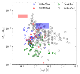
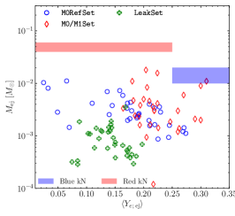
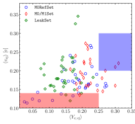
Figure 1: Summary of dynamical ejecta properties used in this work. Blue circles represent models of M0RefSet, red diamonds stands for models from M0/M1Set, green crosses are models from LeakSet and gray squares stand for models from NoNusSet, We show for comparison the two-component fit to AT2017gfo as colored patches from Villar et al. (2017); Siegel (2019).

In total we collect $324$ models. For $271$ of them we have/compute the binary parameters required for the analysis. For all of them the ejecta mass, $M_{\mathrm{e}j}$, is available. For the models in Kiuchi et al. (2019) the ejecta velocity is not reported, thus only for $246$ models the mass-averaged ejecta velocity, $\langle v_{\infty}\rangle$, is given. In addition to NoNusSet models, the average electron fraction of the ejecta is not provided also in Lehner et al. (2016). Hence, there are $99$ models for which the mass-averaged electron fraction of the dynamical ejecta, $\langle Y_{e}\rangle$, is available. Finally, for $76$ models the root mean square (RMS) half opening angle of the outflow about the equatorial plane, $\langle\theta_{\mathrm{R}MS}\rangle$, is available. The disk mass, $M_{\mathrm{d}isk}$, is provided for $119$ models.

Since uncertainties estimates are not available for all datasets, we assign errors following Ref. Radice et al. (2018a), that were motivated by the observed resolution dependency of ejecta properties. Different error measures, if adopted consistently, do not change results qualitatively, as we show in the case of M0RefSet in Appendix C. For the dynamical ejecta mass we consider an uncertainty given by:

$$\Delta M_{\text{ej}}=0.5M_{\text{ej}}+5\times 10^{-5}M_{\odot}.$$ (2)

For the ejecta velocity and for the electron fraction we consider $\Delta\upsilon_{\text{ej}}=0.02$ c and $\Delta Y_{e}=0.01$ as fiducial uncertainties, respectively. The latter value is justified by the robust behavior of the average electron fraction in simulations where multiple resolutions are available .

For the disk mass we assume Radice et al. (2018a)

$$\Delta M_{\text{disk}}=0.5M_{\mathrm{d}isk}+(5\times 10^{-4})M_{\odot}\ .$$ (3)

In this paper we aim to asses (i) the quality of the various fitting formulae to the ejecta properties and the disk mass. Because of the limited number of simulations in datasets, and having in mind multimessenger applications, instead of analyzing each dataset individually, in the main text we employ the following strategy. We study the progressively larger sample of simulations by iteratively adding datasets, starting from M0RefSet. The order in which we add the datasets is governed by the complexity of the physical setup, i.e., M0/M1Set, LeakSet and finally NoNusSet. By progressively including datasets into the analysis we provide a suite of possible calibrations that can either contain the simulations with the most advanced physics input but relatively small number of them (i.e., M0RefSet and M0/M1Set), or all the simulations available. Using the standard statistical methods we rank the fitting formulae and discuss their application. Additionally, we assess (ii) how the progressive inclusion changes the statistical properties of the enlarged set of simulations, aiming to assess the impact that simulating microphysics and neutrino transport has on the ejecta properties. Finally, we elaborate on which fitting formula and what calibration are favorable based on our analysis in the discussion and directly apply it to modeling the key kilonova properties.

For (i) we consider the fitting formulae that exist in the literature as well as new fitting formulae based on simple polynomials in the key BNS parameters i.e., reduced tidal deformability, $\tilde{\Lambda}$, and mass ratio, $q$. Then we perform a standard fitting procedure with least square method, minimizing the residuals and display the fit performance on the residual plots for every quantity. To quantitatively gauge the fit performance (for each ejecta property) we employ the sum of squared residuals (SSR) defined as $\text{SSR}=\sum\limits_{i=1}^{N}(o_{i}-e_{i})^{2}$ and the reduced $\chi^{2}$ statistics:

$$\chi_{\nu}^{2}=\frac{\chi^{2}}{N-C}=\frac{1}{N-C}\sum\limits_{i=1}^{N}\Bigg{(}\frac{o_{i}-e_{i}}{o_{i}^{\mathrm{e}rr}}\Bigg{)}^{2},$$ (4)

where $N$ is the number of points in the dataset, $C$ is the number of coefficients in the fitting model (thus $N-C$ defines the number of degrees of freedom), $o_{i}$ are the dataset values and $o_{i}^{\mathrm{e}rr}$ their errors, $e_{i}$ are the values predicted by the fitting model, and $o_{i}-e_{i}$ are the residuals. The model comparison thus states that the lower SSR is and the closer to $1$ $\chi_{\nu}^{2}$ is, the better the model performs. Note: a fit with the lowest $\chi^{2}_{\nu}$ may not necessarily be the fit with the lowest residuals if the error measure is not constant, e.g.,, for $M_{\mathrm{e}j}$ and $M_{\mathrm{d}isk}$. This allows us to further asses the influence of the error measure.

This procedure is repeated for every dataset added. We provide the calibration for all fitting formulae and for all sets of datasets. We also perform the analysis for all datasets individually. Results, reported in Appendix B corroborate the ones stated in the main text.

For (ii) we employ the following procedure. We start with the set that is uniform in physics and code, the M0RefSet that covers a narrow range in parameter space and allows to establish the base line. Then we add the rest of the models with neutrino heating and cooling effects, the M0/M1Set, and asses how the basic statistical properties have changed, employing the simplest quantitative measure that characterizes a statistical ensemble, and standard deviation. To investigate the effects of the absence of neutrino reabsorption, we add the dataset that does not include this effect, the LeakSet and repeat the analysis. Finally, to asses the effect of the absence of neutrino cooling and differences in the EOS treatment we repeat the analysis with all datasets, including the NoNusSet. This iterative procedure allows to gauge the qualitative effect that different physical treatments have of the statistical behavior of the ejecta parameters and disk mass. We leave a more rigorous quantitative analysis to future works, when larger sample of data with physically motivated error measures and that cover a broader range in parameter space becomes available.

III Dynamical Ejecta

The mechanism behind the production of dynamical ejecta as well as the details on the numerical relativity simulations of M0RefSet are discussed in e.g., Radice et al. (2020); Bernuzzi (2020); Nedora et al. (2021). Here, we focus on overall properties of the mass ejecta in relation to other results in the literature, and provide approximate fitting formulae for the total ejecta mass, the mass-averaged velocity, the electron fraction and the RMS half opening angle. Importantly, the are several criteria for a fluid element to become gravitationally unbound – to become ejecta. Due to the ”burst-like” nature of dynamical ejecta, the geodesic criterion, that considers fluid elements moving on ballistic trajectories, neglecting the fluid pressure Rezzolla and Zanotti (2013), is commonly employed Radice et al. (2016, 2018a); Bernuzzi et al. (2020). Another broadly used criterion is the Bernoulli criterion, that takes into account the internal energy of the fluid. With respect to the dynamical ejecta, these two criteria was found to lead to the ejecta mass estimations different by a factor of $2$ Foucart et al. (2016b). Additionally, depending on the length of the postmerger evolution of a simulation, different methods are employed to compute the ejecta properties. For instance, in Radice et al. (2018a), the ejecta was computed following the matter passing an extraction sphere untill the matter flux subsided. Simulations were sufficiently long to allow the mass flux to saturate. Meanwhile in Vincent et al. (2020), a combination ejecta that was able to leave the simulation domain and that was still within the domain of the simulation at the end was considered. These differences in ejecta criteria and method of calculation present an additional source of systematics in data.

Figure 1 summarizes the total mass, the mass-averaged velocity and mass-averaged electron fraction (where available) for the used datasets. Overall we note that the ejecta properties of the models of M0RefSet are compatible with those of M0/M1Set, as they include the same physics with respect to the EOS treatment and also include the effect of neutrino absorption. Notably, the very high mass-ratio, $q$, models of M0RefSet, discussed in Bernuzzi et al. (2020), show slightly different properties, as their ejecta is of tidal origin only. Comparing the properties of M0/M1Set and LeakSet we observe that neutrino absorption leads, on average, to a larger ejecta mass, which is especially noticeable for the leakage subset of Radice et al. (2018a)(LK). Additionally, neutrino absorption leads to a higher $\langle Y_{e}\rangle$ of the ejecta, while the average velocity, $\langle v_{\infty}\rangle$, appears to be independent of it.

In the following we discuss the fitting formulae for the different quantities.

III.1 Mass

In order to asses the systematic changes in ejecta masses between different datasets with different physics input, we restrict the binary parameter space to $q\in(1,1.2)$ and $\tilde{\Lambda}\in(350,850)$, common for all datasets that we compare. In doing so we reduce the number of simulations significantly. Thus, we aim to assess the changes on the qualitative level only. A more rigorous analysis would require significantly larger sample of simulations, homogeneously distributed in the parameter space. The dynamical ejecta mass, averaged over $8$ simulations of M0RefSet is $\overline{M_{\mathrm{e}j}}=(3.5\pm 1.3)\times 10^{-3}M_{\odot}\,$ where hereafter we report also the standard deviation computed over the relevant simulation sample .

Adding the rest of M0/M1Set (7 models) we obtain $(5.1\pm 3.9)\times 10^{-3}M_{\odot}$. The increase is given largely by datasets that include the M1 neutrino scheme, Vincent et al. (2020) and Sekiguchi et al. (2016). However, adding models of LeakSet, (another 8 models) we observe that the mean value decreases to $3.8\times 10^{-3}M_{\odot}$, as models without neutrino absorption predict, on average, lower ejecta masses. Finally, adding models without neutrinos at all, some of which have polytropic EOS (7 models in the restricted parameter space), we do not observe change in the $\overline{M_{\mathrm{e}j}}$.

Lifting the restrictions on the parameter space, we fit all the available data using second-order polynomials in one parameter $(\tilde{\Lambda})$, and in two parameters, $(q,\tilde{\Lambda})$, namely:

$$P_{2}^{1}(\tilde{\Lambda}) =b_{0}+b_{1}\tilde{\Lambda}+b_{2}\tilde{\Lambda}^{2},$$ (5)

$$P_{2}^{2}(q,\tilde{\Lambda}) =b_{0}+b_{1}q+b_{2}\tilde{\Lambda}+b_{3}q^{2}+b_{4}q\tilde{\Lambda}+b_{5}\tilde{\Lambda}^{2}\,.$$ (6)

Additionally, we consider the fitting model presented Refs. Kawaguchi et al. (2016); Dietrich and Ujevic (2017); Radice et al. (2018a)

$$\left(\frac{M_{\mathrm{e}j}}{10^{-3}M_{\odot}}\right)_{\mathrm{f}it}=\Big{[}\alpha\Big{(}\frac{M_{B}}{M_{A}}\Big{)}^{1/3}\Big{(}\frac{1-2C_{A}}{C_{A}}\Big{)}+\beta\Big{(}\frac{M_{B}}{M_{A}}\Big{)}^{n}$$ (7)

$$+\gamma\Big{(}1-\frac{M_{A}}{M_{b\,A}}\Big{)}\Big{]}M_{b\,A}+(A\leftrightarrow B)+\delta,$$

and the model presented in Krüger and Foucart (2020):

$$\left(\frac{M_{\mathrm{e}j}}{10^{-3}M_{\odot}}\right)_{\mathrm{f}it}=\left(\frac{\alpha}{C_{A}}+\beta\frac{M_{B}^{n}}{M_{A}^{n}}+\gamma C_{A}\Bigg{)}M_{A}+(A\leftrightarrow B)\right.\ .$$ (8)

As in some cases the values of $M_{\mathrm{e}j}$ change by orders of magnitude for very close values of $q$ and $\tilde{\Lambda}$, we calibrate the fitting models to $\log_{10}(M_{\mathrm{e}j})$ instead of the $M_{\mathrm{e}j}$.

Regarding Eq. (7) and Eq. (8), we also note that these formulae deliver ill-conditioned fits, with coefficients that change up to a factor of two for the same data, depending on the guesses or on the nonlinear fitting algorithm employed. While such formulae may allow to account for a non-smooth behavior in data, their calibration presents an additional challenge.

Fitting coefficients as well as values of $\chi^{2}_{\nu}$ are reported in Appendix A: coefficients of the polynomial regressions are reported in Tab. 4; fits coefficients for Eqs.(7)-(8) are reported in Tab. 5.

Table 2: Values of SSR for different fitting models for the dynamical ejecta properties. Mean is the simulation average, $P_{n}(x,y)$ is a polynomial of order $n$ in the variables $x,y$. Fits are performed for the data of this work and for an increasingly larger combined dataset from the literature. See text for discussion. The best fitting model for a given dataset is characterized by the lowest value of SSR.

$\log_{10}(M_{\mathrm{e}j})$	Datasets	Mean	Eq. (7)	Eq. (8)	$P_{2}^{1}(\tilde{\Lambda})$	$P_{2}^{2}(q,\tilde{\Lambda})$
	M0RefSet	2.57	1.65	1.40	2.43	0.97
	& M0/M1Set	8.19	7.51	6.35	7.84	6.55
	& LeakSet	33.13	26.37	21.57	29.62	24.40
	& NoNusSet	86.93	80.08	63.38	86.85	55.09
$\langle v_{\mathrm{e}j}\rangle$	Datasets	Mean	Eq. (9)		$P_{2}^{1}(\tilde{\Lambda})$	$P_{2}^{2}(q,\tilde{\Lambda})$
	M0RefSet	0.04	0.02		0.04	0.01
	& M0/M1Set	0.09	0.05		0.07	0.04
	& LeakSet	0.29	0.24		0.25	0.21
	& NoNusSet	0.78	0.66		0.74	0.67
$\langle Y_{\mathrm{e}}\rangle$	datasets	Mean			$P_{2}^{1}(\tilde{\Lambda})$	$P_{2}^{2}(q,\tilde{\Lambda})$
	M0RefSet	0.14			0.13	0.02
	& M0/M1Set	0.24			0.23	0.06
	& LeakSet	0.35			0.35	0.23
$\langle\theta_{\mathrm{R}MS}\rangle$	datasets	Mean			$P_{2}^{1}(\tilde{\Lambda})$	$P_{2}^{2}(q,\tilde{\Lambda})$
	M0RefSet	2775			2631	498
	& M0/M1Set	2949			2788	574
	& LeakSet	4681			4116	2382

Different fits for the dynamical ejecta properties are compared in terms of the sum of squared residuals, SSR, in Tab. 2. We find that fitting the data from only M0RefSet as well as all the data from all datasets combined, the lowest SSR is given by $P_{2}^{2}(q,\tilde{\Lambda})$. The Eq. (8) gives similar, albeit slightly larger values for these sets of simulations, while performing slightly better for the other two combinations of datasets. Invoking the error measure and the $\chi^{2}_{\nu}{}$ statistic we observe a very similar picture with $P_{2}^{2}(q,\tilde{\Lambda})$ giving the lowest $\chi^{2}_{\nu}$ when all datasets are considered and Eq. (8) performing better when only M0/M1Set and M0RefSet are considered. The small difference in performance between these two fitting formulae can be attributed to the fact that both include the mass ratio explicitly, which allows to capture the leading trend in the data.

The Eq. (7) cannot sufficiently well reproduce the low ejecta masses of models with microphysic EOS and leakage neutrino transport scheme and high ejecta masses of models with polytropic EOS and no neutrino transport. This results in the truncated $M_{\mathrm{e}j;fit}$ (see Fig. 2) and larger SSR and $\chi^{2}_{\nu}$. In addition, it was previously found in Radice et al. (2018a), that this fit model does not accurately reproduce the data and misses systematic trends. The simplest model, a polynomial of only $\tilde{\Lambda}$, cannot capture leading trends in the data, resulting in considerably larger SSR and $\chi^{2}_{\nu}{}$ once all datasets are considered. Similarly, taking the simple mean value as a fitting model results in an even larger SSR and $\chi^{2}_{\nu}$. Thus, the inclusion of the dependency on mass-ratio is of crucial importance for modeling dynamical ejecta mass.

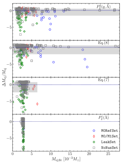
Figure 2: Relative differences between data and fits for the dynamical ejecta mass, $\Delta M_{\mathrm{e}j}=M_{\mathrm{e}j}-M^{\mathrm{f}it}_{\mathrm{e}j}$. We show polynomial fits and fitting formulae Eq. (7) and Eq. (8) calibrated with all datasets available. From top to bottom the models arrange based on their SSR: from lowest to highest See Tab. 2. The gray region represents the fit’s $68\%$ confidence level. Note that fitting was performed minimizing $\log_{10}(M_{\mathrm{e}j})$. See text for details.

In Fig. 2 we show the relative differences between all datasets values and values from the fitting models. We observe that none of the fitting models can adequately capture the subset of LeakSet with a leakage scheme only as neutrino treatment, (Cf. Radice et al. (2018a); Lehner et al. (2016)). While the lowest SSR and $\chi^{2}_{\nu}{}$ are found for $P_{2}^{2}(q,\tilde{\Lambda})$, the plot shows that the Eq. (8) can also capture the large ejecta mass of NoNusSet and M0RefSet with however higher residuals. Notably Eq. (7) cannot capture that tail, truncating the distribution at $\sim 10^{-2}M_{\odot}$. The polynomial in $\tilde{\Lambda}$ fits the data very poorly, showing an almost flat distribution around the mean value of the ejecta mass.

III.2 Mass-averaged velocity

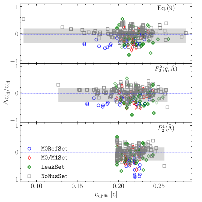
Figure 3: Relative differences between data and fits for the mass-averaged velocity of the dynamical ejecta, $\Delta\upsilon_{\mathrm{e}j}=\upsilon_{\mathrm{e}j}-\upsilon^{\mathrm{f}it}_{\mathrm{e}j}$. Calibration is done for all datasets available. We show the fitting formula Eq. (9) and the polynomial fits. From top to bottom the models are arranged based on their $\chi^{2}_{\nu}{}$: from lowest to highest.

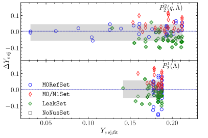
Figure 4: Relative differences between data and fits for the mass-averaged electron fraction of the dynamical ejecta. We show the polynomial fits, and Eq. (5) and Eq. (6). Calibration is done for all datasets available. Here $\Delta Y_{e\>\mathrm{e}j}=Y_{e\>\mathrm{e}j}-Y^{\mathrm{f}it}_{e\>\mathrm{e}j}$. From top to bottom the models are arranged based on their $\chi^{2}_{\nu}{}$: from lowest to highest.

The mass-averaged terminal velocity of the dynamical ejecta, $\langle v_{\infty}\rangle$, from M0RefSet ranges from $0.11\,c$ to $0.27\,c$, in agreement with the leakage simulations performed with the same code in Radice et al. (2018a). However, differently from the analysis of Radice et al. (2018a), the correlation of the $\langle\upsilon_{\infty}\rangle$ with the tidal parameter $\tilde{\Lambda}$ was found in the models of M0RefSet with the fixed chirp mass Nedora et al. (2021). Models with lower $\tilde{\Lambda}$, showed higher velocities. This is a consequence of the fact that the dynamical ejecta in comparable-mass mergers are dominated by the shocked component and that the shock velocity is larger the more compact the binary is. On the contrary, for high mass ratios $q\gtrsim 1.5$, the ejecta are dominated by the tidal component and a larger $q$ leads to a smaller $\langle v_{\infty}\rangle$ in M0RefSet.

Restricting the parameter space again, we asses the change in mean value of ejecta velocity, $\overline{\langle v_{\infty}\rangle}$. For the models of M0RefSet we find $\overline{\langle v_{\infty}\rangle}=0.19\pm 0.03\,c$. When we iteratively add models of M0/M1Set, LeakSet and NoNusSet, the $\overline{\langle v_{\infty}\rangle}$ remains largely unchanged, taking values of $0.20\,c$, $0.20\,c$ and $0.21\,c$. Notably, Fig. 1, shows that some models of NoNusSet (models of Cf. Bauswein et al. (2013) ) have an overall larger velocity. However, they lie outside of the restricted parameter space.

Lifting the restrictions on the parameter space we fit the data with a second-order polynomials, as in Eq. (5), and also with the fit formula reported in Dietrich et al. (2017); Radice et al. (2018a):

$${\langle v_{\infty}\rangle}_{\mathrm{f}it}=\Big{[}\alpha\Big{(}\frac{M_{A}}{M_{B}}\Big{)}(1+\gamma C_{A})\Big{]}+(A\leftrightarrow B)+\beta\,.$$ (9)

We note, that similarly to the Eq. (7) and Eq. (8), the outcome of the calibration of the Eq. (9) depends on the initial guesses of the minimization algorithm.

The coefficients of the polynomial regressions for $\langle v_{\infty}\rangle$ are reported in Tab. 4; fits coefficients for Eq. (9) are reported in Tab. 5. The fit models’ performance is summarized in Tab. 2 in terms of SSR.

We find that unless models of NoNusSet are included, the $P_{2}^{2}(q,\tilde{\Lambda})$ displays the lowest SSR and $\chi^{2}_{\nu}{}$ among other fitting formulae. When models of NoNusSet are also included, the $P_{2}^{2}(q,\tilde{\Lambda})$ and Eq. (9) perform rather similar.

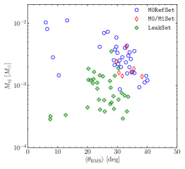
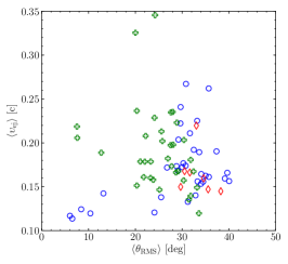
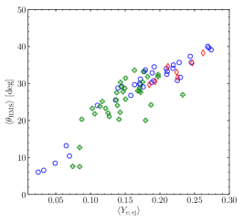
Figure 5: Relations between the ejecta $\theta_{\mathrm{R}MS}$ and other parameters of the dynamical ejecta: mass, $M_{\mathrm{e}j}$, velocity, $\langle v_{\infty}\rangle$, and electron fraction $\langle Y_{e}\rangle$ for models from M0RefSet and Radice et al. (2018a) from LeakSet and M0/M1Set. Plots show that models with neutrino absorption have higher $M_{\mathrm{e}j}$ and larger $\theta_{\mathrm{R}MS}$ as well as a clear correlation between $\theta_{\mathrm{R}MS}$ and $\langle Y_{e}\rangle$.

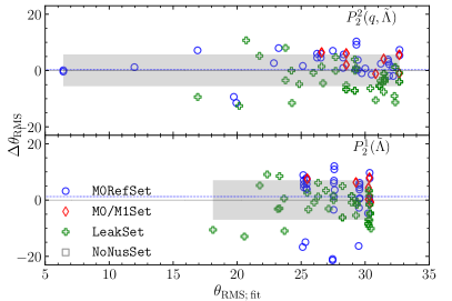
Figure 6: Relative differences between data and fits of dynamical ejecta mass-averaged electron fraction. We show polynomial fits only. Here $\Delta\theta_{\mathrm{R}MS}=\theta_{\mathrm{R}MS}-\theta^{\mathrm{f}it}_{\mathrm{R}MS}$. From top to bottom the models are arranged based on their $\chi^{2}_{\nu}$: from lowest to highest.

In Fig. 3 we show the differences between the data and the fits for the considered fitting models. We find that Eq. (9) and the second order polynomial in ($q,\tilde{\Lambda}$) reproduce most of the data within an error of $\sim 50\%$ and overall perform very similarly. In both cases, the largest deviations are obtained for models of the LeakSet, with the neutrino leakage scheme. The one parameter polynomial of $\tilde{\Lambda}$ fails to capture the low velocity tail of the distribution and overall gives considerably higher differences between the dataset and the model predicted values of $\langle v_{\infty}\rangle$.

III.3 Electron fraction

The mass-averaged electron fraction, $\langle Y_{e}\rangle$, in M0RefSet varies from $0.03$ to $0.27$.

Restricting the parameter space to the common region, we obtain the mean value of electron fraction for M0RefSet $\overline{\langle Y_{e}\rangle}=0.19\pm 0.02$. Adding models of M0/M1Set increases the mean to $0.20\pm 0.04$ which is largely due to models of Sekiguchi et al. (2015, 2016) with leakage+M1 scheme (see Fig. 1). When models of the LeakSet are added, the mean values decreases back, which is as expected as models with leakage scheme only have lower ejecta electron fraction e.g.,, Radice et al. (2018a). Notably, the number of simulations added is rather small .

Regarding the fitting functions, we explore the low-order polynomials in $(q,\tilde{\Lambda})$ and in $(\tilde{\Lambda})$ only. The coefficients of polynomial regressions are reported in Tab. 4. We observe that for all datasets, the $P_{2}^{2}(q,\tilde{\Lambda})$ displays consistently lower SSR and $\chi^{2}_{\nu}{}$. Notably, the addition of LeakSet models leads to a jump in these measures, as the data in this set is statistically different (different physics setup). In Fig. 4 we show the performance of the different fitting models for the mass-averaged electron fraction of the ejecta. When all datasets are considered, the second order polynomial manages to reproduce both the low-$Y_{e}$ tail and high $Y_{e}$ values for models with advanced neutrino treatment. The accurate computation of the electron fraction naturally requires neutrino absorption to be included into simulation setups. The availability of a larger number of simulations with advanced neutrino transport will undoubtedly improve fitting models.

III.4 Root mean square half opening angle

Ejecta geometry was found to have a strong imprint on the properties of the electromagnetic counterparts to mergers (e.g., Perego et al., 2017). Numerical relativity simulations show that the form of the angular distribution of ejecta properties is quite complex (e.g., Radice et al., 2018a) and presents challenges for a statistical analysis. Here we employ the mass-averaged RMS half opening angle (under the assumption of axial symmetry), a quantity that can be used to separate the massive, low-latitude outflow and less massive, polar one. In the Discussion we show an example of how this quantity can be used in kilonova modeling. Following Radice et al. (2018a), we define the mass-averaged RMS half opening angle as by assuming axial symmetry and computing:

$$\theta_{\mathrm{R}MS}=\frac{180}{\pi}\Bigg{(}\frac{\sum m_{i}\theta_{i}^{2}}{\sum m_{i}}\Bigg{)}^{1/2}\,,$$ (10)

where $\theta_{i}$ and $m_{i}$ are the angle (from the binary plane) and mass of the ejecta element. This quantity is available only for M0RefSet and for the models of Radice et al. (2018a). In Figure 5 we show the dependency of $\theta_{\mathrm{R}MS}$ on the previously discussed ejecta parameters. Comparing the data from M0RefSet and the leakage dataset of Ref. Radice et al. (2018a), we find that the inclusion of neutrino absorption leads to larger $\theta_{\mathrm{R}MS}$ on average with the exception of highly asymmetric models of M0RefSet. Notably we observe a clear linear relation between the $\theta_{\mathrm{R}MS}$ and $\langle Y_{e}\rangle$ (see Fig. 5). The origin of this relation lies in the dependency of the ejecta properties on the binary mass-ratio. Asymmetric binaries produce low-$Y_{e}$, tidal ejecta confined largely to the lane of the binary, while for more symmetric models with prominent shocked ejecta component there is a trend to have higher $Y_{e}$ and more spread-out ejecta. This further suggests that $\theta_{\mathrm{R}MS}$ can help capturing the transition between the low- and high-opacity ejecta in kilonova modeling.

The number of models within the restricted parameter space for which we have the $\theta_{\mathrm{R}MS}$ is very limited. Thus we only report the average value for M0RefSet, $\overline{\langle\theta_{\mathrm{R}MS}\rangle}=(31.7\pm 1.9)~{}\text{deg}$.

In light of the considerably smaller sample of models for which we have $\theta_{\mathrm{R}MS}$, we simplify the statistical analysis, considering as fitting models only polynomials: $P_{2}^{1}(\tilde{\Lambda})$ and $P_{2}^{2}(q,\tilde{\Lambda})$. The coefficients of the polynomial regressions are reported in Tab. 4. Following Radice et al. (2018a) we adopt a uniform error for all models of $2$ degrees. We find that similarly to the case of ejecta electron fraction, the $P_{2}^{2}(q,\tilde{\Lambda})$ performs consistently better here than other options for all datasets in terms of both SSR and $\chi^{2}_{\nu}$.

In Fig. 6 we show the performance of polynomial fitting models to the ejecta $\theta_{\mathrm{R}MS}$. The second order polynomial provides a better fit to the low-$\theta_{\mathrm{R}MS}$ tail of the distribution than $P_{2}^{1}(\tilde{\Lambda})$. and reproduces the data within $\sim 10\,$deg. Overall, we observe that the inclusion of both $q$ and $\tilde{\Lambda}$ in a fitting formula is important for capturing the trends in data. However, the small sample of models does not allow us to conduct a more thorough investigation, in particular, to study the effects of various physics included in simulations.

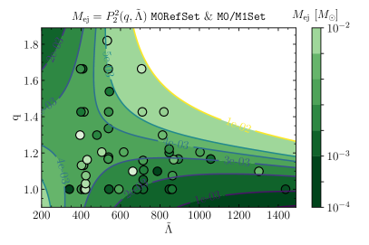
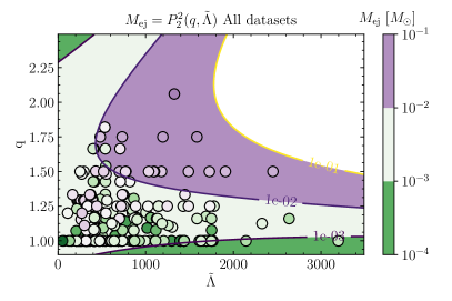
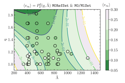
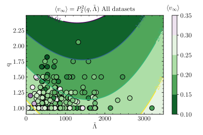
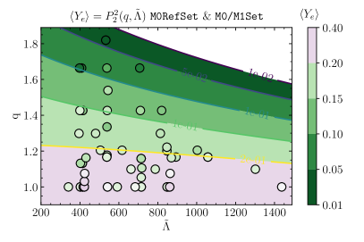
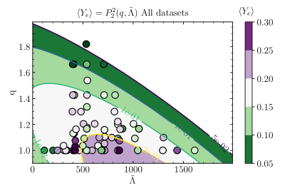
Figure 7: Comparsion between ejecta parameters informed by the fit (colored contours), and the simulation ejecta data (colored markers) for $P_{2}^{2}(q,\tilde{\Lambda})$ fitting model calibrated with advanced-physics datasets, M0RefSet and M0/M1Set, (left column of panels) and with all available datasets (right column of panels). The plot shows that for some physical quantities, such as ejecta electron fraction and velocity, the leading trends in data appear to be captured by the $P_{2}^{2}(q,\tilde{\Lambda})$ calibrated with datasets with advanced physics. When all datasets are considered, however, the limitations of the smooth polynomial fitting function becomes apparent as it is not able to fit the non-smooth data well.

III.5 Application of the polynomial fit

Overall, comparing the performance of different fitting formulae to the ejecta properties, we find that the $P_{2}^{2}(q,\tilde{\Lambda})$ gives a comparatively better fit when all simulation data from all datasets are considered. When only the M0RefSet and M0/M1Set are considered, however, the ejecta mass is slightly better fitted by non-polynomial fitting formula, Eq. (8). The implicit inclusion of mass-ratio allows the $P_{2}^{2}(q,\tilde{\Lambda})$ to capture leading trends in the behaviour of $\langle v_{\infty}\rangle$, $\langle Y_{e}\rangle$ and $\theta_{\mathrm{R}MS}$. For its calibration we suggest datasets with the most advanced physics i.e., M0/M1Set and M0RefSet. A caution must be exercised when using datasets computed with different physics input and at various resolutions, as in certain cases (e.g., $M_{\mathrm{e}j}$), the systematics introduced by these differences might obscure the leading trends in data. This conclusion is supported by the analysis of the statistical behaviour of data from different datasets and further corroborated by the analysis of the individual datasets (see Appendix B). In addition to the quantitative and qualitative assessments of the fit performance via SSR, $\chi^{2}_{\nu}$-statistics and residual plots, we consider a direct application of the, $P_{2}^{2}(q,\tilde{\Lambda})$ and compare it to the data used for calibration in Fig. 7. The plot shows that the behaviour of the fitting formula depends sensibly on the choice of datasets used for calibration, and the predictive power of the fit reduces when datasets with different physics (the difference in contour shapes between left and right column of subplots) and numerical setups are employed. The ejecta properties, especially, mass, velocity and electron fraction depend strongly on the neutrino treatment scheme and larger number of high resolution NR simulations with advanced treatment of neutrino emission and absorption is required to further constrain the statistics of ejecta properties.

IV Remnant disk

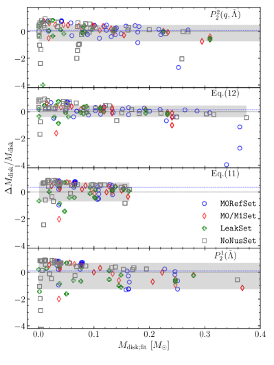
Figure 8: Relative differences between data and the fits of the disk mass. The calibration was performed for $\log_{10}(M_{\mathrm{d}isk})$ using simulations from all datasets. Different panels show polynomial fits in $\tilde{\Lambda}$ and $(q,\tilde{\Lambda})$, fitting formulae Eq. (7) and Eq. (8). The best fitting model is characterized by the lowest value of $\chi_{\nu}^{2}$. Best fitting coefficients are given in the tables in Appendix A. Here $\Delta M_{\mathrm{d}isk}=M_{\mathrm{d}isk}-M^{\mathrm{f}it}_{\mathrm{d}isk}$. The fitting procedure here was based in minimizing residuals instead of $\chi_{\nu}^{2}$ as otherwise, the error measure adapted, Eq. (3), would lead to the fit underestimating most of datasets used.

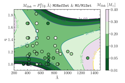
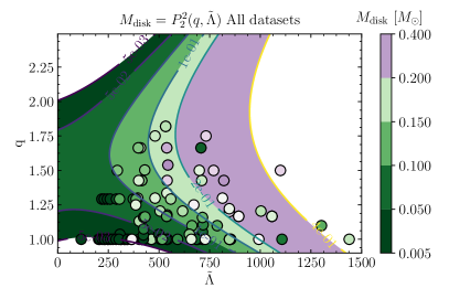
Figure 9: Same as Fig. 7 but for the disk mass. The plot shows that at low values of $q$ and $\tilde{\Lambda}$ the fit is able to capture the leading trends in data. However, in the region where there are fewer data preset, at high $q$ and $\tilde{\Lambda}$, the fit becomes increasingly less accurate (see text).

Table 3: Sum of squared residuals for different fit models for the final disk mass, $\log_{10}(M_{\mathrm{d}isk})$.

datasets	Mean	Eq. (11)	Eq. (12)	$P_{2}^{1}(\tilde{\Lambda})$	$P_{2}^{2}(q,\tilde{\Lambda})$
M0RefSet	15.11	13.28	9.96	13.95	8.81
& M0/M1Set	17.03	14.42	11.58	15.24	10.70
& LeakSet	54.02	32.56	17.65	29.72	19.56
& NoNusSet	80.47	45.71	30.06	44.04	26.73

The disk mass at the end of the simulation of models of M0RefSet varies from $0.01M_{\odot}$ to $0.3M_{\odot}$. Within the restricted parameter space the mean value of the disk mass, $\overline{M_{\mathrm{d}isk}}$, for models of the M0RefSet is $(0.12\pm 0.05)M_{\odot}$ and it decreases only slightly when models from M0/M1Set, LeakSet are added, to $(0.11\pm 0.04)M_{\odot}$. Notably, large variations in the mean value are observed when the parameter space is enlarged to include very asymmetric and promptly collapsing models. However, there is not enough models for the comparison. While this might suggest that the disk mass depends weakly on the physical setup of simulations, the large uncertainties in data and the fundamental difference between the disk around a neutron star and a black hole must be taken into consideration. In particular, we stress that the disk mass is estimated in different ways in the different datasets. In Dietrich et al. (2015, 2017) the disk is estimated only for BNS forming BH, at approximately ${\approx}1$ ms after collapse and computing the rest mass outside the apparent horizon (AH). In Sekiguchi et al. (2016), the disk mass is extracted at ${\approx}30$ ms outside the AH. In Radice et al. (2018a), the disk mass is computed as the baryonic mass outside the AH at BH formation, while for NS remnants the criterion $\rho<10^{13}$ g cm^-3 is used. In Kiuchi et al. (2019) for both BH and NS outcome the $\rho<10^{13}$ g cm^-3 criterion is used and time of the extraction is not specified. In Vincent et al. (2020) the density criterion is the same, however the simulations are significantly shorter (${\sim 7.5}$ ms) than in other works. Overall, we estimate that these differences can amount to a systematic factor of a few.

As fitting formulae we consider the polynomials Eqs (5) and (6), and the formula provided in Radice et al. (2018a):

Similarly to the mass of dynamical ejecta, the disk mass varies by up to an order of magnitude for, in some cases, very similar values of $q$ and $\tilde{\Lambda}$. In order to simplify the fitting procedure and reproduce both, high and low mass tails, we consider the $\log_{10}(M_{\mathrm{d}isk})$. Notably, the Eqs. (11)-(12) are segmented, and include constant parts. For clarity we write the equations in the form used for fitting, that read

$$\begin{split}\log_{10}\left(\frac{M_{\mathrm{disk}}}{M_{\odot}}\right)_{\mathrm{f}it}&\\ =\text{max}\Big{\{}-3.0,\,\log_{10}\Big{(}\alpha&+\beta\tanh\Big{(}\frac{\tilde{\Lambda}-\gamma}{\delta}\Big{)}\Big{)}\Big{\}}\,,\end{split}$$ (11)

and the fitting formula provided in Krüger and Foucart (2020):

$$\begin{split}\log_{10}\left(\frac{M_{\mathrm{disk}}}{M_{\odot}}\right)_{\mathrm{f}it}&\\ =\log_{10}(M_{A})+\text{max}\Big{\{}-3.30,\,&\log_{10}\Big{(}(\alpha C_{A}+\beta)^{\gamma}\Big{)}\Big{)}\Big{\}}\,.\end{split}$$ (12)

The exact from of polynomials, $P_{2}^{1}(\tilde{\Lambda})$ and $P_{2}^{2}(q,\tilde{\Lambda})$, used in this section than reads,

$$\log_{10}\left(P_{2}^{1}(\tilde{\Lambda})\right) =\log_{10}\Big{(}b_{0}+b_{1}\tilde{\Lambda}+b_{2}\tilde{\Lambda}^{2}\Big{)},$$

$$\log_{10}\left(P_{2}^{2}(q,\tilde{\Lambda})\right) =\log_{10}\Big{(}b_{0}+b_{1}q+b_{2}\tilde{\Lambda}+b_{3}q^{2}$$

$$+b_{4}q\tilde{\Lambda}+b_{5}\tilde{\Lambda}^{2}\Big{)}\,.$$

As before we opt here for the minimization of residuals in the fitting procedure. We rank the fitting formulae performance based on the SSR, augmenting the dicsusion with $\chi^{2}_{\nu}$, computed using the error measure (3).

The coefficients of the polynomial regressions are reported in Tab. 6; the fit coefficients for Eq. (11) and Eq. (12) are reported in Tab. 7. The SSR for these fits are reported in Tab. 3. As for those for the dynamical ejecta, the formulae in Eq. (11) and Eq. (12) give ill-conditioned fits. Notably, we find that depending on the initial guess for coefficients the Eq. (12) may develop singularities when data from all datasets is fitted and no limitations are imposed upon the coefficients. However, such non-smooth fitting functions may allow to capture the complex behavior in data, not reproduced by $P_{2}^{1}(\tilde{\Lambda})$ and $P_{2}^{2}(q,\tilde{\Lambda})$

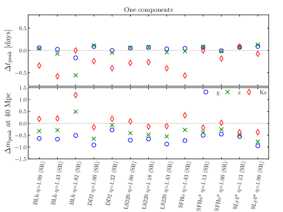
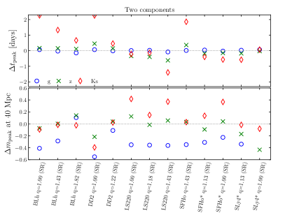
Figure 10: Comparison between one component light curves (left panel) and two components light curves (right panel) in $g$, $z$ and $K_{s}$ bands using direct NR input or the fitting formulae for the dynamical ejecta and disk mass. The $y-$axis displays the difference between the peak time (top panel), $\Delta t_{\mathrm{p}eak}=t_{\mathrm{p}eak;NR}-t_{\mathrm{p}eak;fit}$, and peak magnitude, $\Delta m_{\mathrm{p}eak}=m_{\mathrm{p}eak;NR}-m_{\mathrm{p}eak;fit}$, (bottom panel); the $x-$axis shows selected BNS models of M0RefSet. The fits employed here are the polynomials in $(q,\tilde{\Lambda})$ used with the best fitting coefficients, calibrated to M0/M1Set (that includes M0RefSet). The plot shows that the light curves generated with the dynamical ejecta fits (one component) tend to underestimate the peak times and magnitudes of NR-informed light curves, especially in the $K_{s}$ band. In case of dynamical ejecta and disk wind (two components) light curves, the peak time is less constrained ($\pm 2$ days) in the $K_{s}$ band, but the peak magnitudes is predicted more accurately $\pm 0.5$ mag.

Fitting the data of M0RefSet and combined M0RefSet dataset and M0/M1Set we observe that the $P_{2}^{2}(q,\tilde{\Lambda})$ consistently shows the lowest SSR and $\chi^{2}_{\nu}{}$. Notably, the Eq. (12) gives only slightly higher values in both cases. When all models from all datasets are considered, we again observe that the $P_{2}^{2}(q,\tilde{\Lambda})$ is statistically preferred with Eq. (12) being the close second. The observed similarity in fitting formulae performance further suggests that indeed mass-ratio and $\tilde{\Lambda}$ allow to capture the main trends in the disk mass data.

When performing the calibration of Eq. (12) and Eq. (11) with standard least-square method we observed that the result of the calibration depends strongly on the initial guesses for the coefficients. This behavior makes the use of these fitting formulae difficult from the point of view of the reproducible of result. We also note that Eqs. (11)-(12) include constant “floor values”. The physical motivation behind these constants is not very clear and while they might help to constrain the fit behaviour at known limits of the parameter space, e.g.,, at $\Lambda\rightarrow 0$, their applicability for all datasets may not be optimal. The $P_{2}^{2}(q,\tilde{\Lambda})$ fitting formula is free from aforementioned issues and allows for stable and reproducible fits.

In Fig. 8 we show the relative differences between the data and the values given by the fitting models. Here the relative performance of the fits can be inferred from the $67\%$ confidence level bar. We observe that the Eq. (11) cannot reproduce the high disk masses found in asymmetric binaries of M0RefSet. Meanwhile other fitting formulae can reproduce both the low and the large disk masses with varying degree of success. Notably, the fit with Eq (12) displays the smallest residuals, i.e., with the narrowest $67\%$ confidence level bar. The second best fit here is $P_{2}^{2}(q,\tilde{\Lambda})$. The reason why the $\chi^{2}_{\nu}$ for the Eq. (12) is larger than that for $P_{2}^{2}(q,\tilde{\Lambda})$ (see Tab. 3) lies in the error measure, Eq. (3), that is used only in $\chi^{2}_{\nu}$ calculation. Thus, while the fit with lowest $\chi^{2}_{\nu}$ provides a better fit for lower disk masses (with tighter errors), the Eq. (12) gives a fit with overall smaller residuals.

We show the performance of the $P_{2}^{2}(q,\tilde{\Lambda})$ fitting formula in the $q$-$\tilde{\Lambda}$ space in Fig. 9. The plot shows that certain main trends in data, e.g., higher disk mass in low-$q$, low-$\tilde{\Lambda}$ simulations, are reproduced by the fit calibrated with either combined M0RefSet and M0/M1Set or all datasets. However, being a smooth function, the $P_{2}^{2}(q,\tilde{\Lambda})$, cannot capture the rapid oscillations in data.

Overall, the statistical analysis shows that the value of the disk mass is subjected to large uncertainties, that include systematic and method-of-computation uncertainties. The leading trends in the data appears to be captured by the fitting formulae that include mass-ratio and reduced tidal deformability. This result is generally supported by the datasets separate statistical analysis (see Appendix B). As a simple polynomial in terms of mass ration and the reduced tidal deformability shows similar or better residuals and $\chi^{2}_{\nu}$, compared to other fitting formulae available in the literate literature and formulated in terms of other binary parameters, we conclude that the former two quantities describe the leading trends in data. The analysis of all datasets individually generally confirms this conclusion, further suggesting that both $P_{2}^{2}(q,\tilde{\Lambda})$ and Eq. (12) perform similarly well (see Appendix B).

V Discussion

In this paper we considered numerical relativity datasets available in the literature for the dynamical ejecta properties and the remnant disk mass from binary neutron star mergers. We performed a simple statistical analysis of the ejecta parameters that highlighted that the ejecta parameters are subjected to large systematic uncertainties, partially due to different treatment of neutrinos, in addition to the EOS formulations. We also compared different fitting formulae for the ejecta properties and disk mass and found that fitting formulae that include the reduced tidal parameter and mass ratio can relatively well reproduce the leading trends in certain datasets with more uniform physics input. In particular, low order polynomials in these quantities provide a simple description of the data available and also favorably compare to the other options in terms of sum of squared residuals when only models of M0RefSet are considered as well or models from all datasets. Large values of SSR and $\chi^{2}_{\nu}{}$ as well as wild oscillations of fitting coefficients for a given quantity between calibrations (see App. A) further indicate the limitations on the ability of the set of all simulations to preserve physical information. This calls for more detailed studies of error estimates in simulations containing the necessary physics. Additionally, a larger sample of simulations with parameters more uniformly distributed is required as the current set available in the literature is rather limited in terms of mass and mass-ratio, and mostly concentrated around binaries with fiducial $1.4{\mathrm{M}_{\odot}}$ NS. Nonetheless, since these fitting formulas are widely used for multimesseneger analyses, we propose the use of these polynomial models instead of other fitting formulae presented in the literature (and also considered in this work) because most of these formulae lead to ill-conditioned fits. Specifically, we recommend the Eq. (6) calibrated with datasets with the most advanced physics input, i.e., M0/M1Set and M0RefSet (highlighted rows in Tab. 4 and Tab. 6) We empathize that the application of the fitting formulae, especially polynomials, should be limited to the parameter space where they have been calibrated. Additionally, while our analysis suggests that for the currently available data, the second order polynomials in $q$ and $\tilde{\Lambda}$ perform comparatively well, higher-order formulae might be necessary to capture the true physics of mergers. We leave their exploration to future works when more simulation data becomes available.

When all data from all available datasets are considered, the fitting formulae with the best statistical performance among those considered are able to reproduce the dynamical ejecta velocity typically to ${\sim}50\%$, with the $68\%$ significance range being $\Delta v_{\infty}/v_{\infty}\in(-0.4,0.2)$. The electron fraction is reproduced with an accuracy of ${\sim}0.1$. The ejecta RMS half opening angle about the orbital plane is reproduced with an accuracy of ${\sim}10$ deg. The ejecta and disk masses, however, are rather uncertain having $(-0.8,0.2)$ and $(-0.4,0.2)$ $68\%$ significance ranges respectively. The smooth fitting formulae can reproduce these quantities to a factor of ${\sim}2$.

The main conclusion of this work is that the currently available data on the ejecta properties and disk masses from binary neutron star mergers contains large systematic uncertainties. Different treatments of EOS and neutrino transport, as well as different resolutions, and methods of calculation of ejecta and disk properties lead to large systematic differences between various datasets. As neutrino re-absorption is a crucial component for reliable estimates of the dynamical ejecta mass, e.g. Wanajo et al. (2014); Sekiguchi et al. (2015); Perego et al. (2017); Foucart et al. (2018), it is of paramount importance to enlarge the M0/M1Set and refine the statistics of ejecta properties. Additionally, different methodologies used to extract and compute these quantities contribute to the uncertainties. Simulations of sequences of binaries at different chirp masses could also be useful to identify new trends in the data that cannot be currently explored. The statistical analysis that we have performed is further subjected to biases as the data in different datasets span different ranges in parameter space of the binary. Considerably larger sets of simulations that cover the parameter space more uniformly are need to alleviate these biases.

Fitting formulae to the ejecta properties and disk mass are commonly used to study sources of the gravitational waves and electromagnetic counterparts. However, caution ought to be exercised when applying the fitting formulae presented here to infer the source parameters from observations.

As an example, we discuss the impact of using our recommended, $P_{2}^{2}(q,\tilde{\Lambda})$, fitting formula for the computation of synthetic kilonova light curves as opposed to the direct numerical relativity input. We use the semi-analytic model of Ref. Perego et al. (2017) with one or two kilonova components, i.e., the dynamical ejecta and the disk wind. We consider a set of selected BNS models from the M0RefSet with 5 different EOS and several mass rations between $q=1.00$ and $q=1.82$. From the $P_{2}^{2}(q,\tilde{\Lambda})$ we estimate the dynamical ejecta mass and velocity and angle separating the low opacity polar part and high opacity part about the plane of the binary, using the $\theta_{\mathrm{R}MS}$ as a separation angle. We invoke the ejecta mass-averaged RMS half opening angle to separate the low-altitude high opacity part and the low-opacity polar part. This allows us to include the change in ejecta geometry with binary parameters. For the secular ejecta mass we assume it to be $40\%$ of the disk mass, evaluated from the best fitting formula. The opacities, heating rates and extrinsic parameters are kept fixed in the comparison.

The results are collected in Fig. 10, where we show peak times and peak magnitudes for the $g$, $z$, and $K_{s}$ filters. In the one component case (left panels), we find that the peak times are reproduced on average within ${\sim}0.2$ days in the $g$ an $z$ bands, and within ${\sim}0.5$ days in $K_{s}$ band. The latter is systematically underestimated. The highly asymmetric binary $q=1.8$ and BLh EOS shows overall the largest deviations. Peak magnitudes in the three bands computed with the fitting formulae differ by ${\sim}0.5$ mag from the NR informed ones, reaching ${\sim}1$ mag in the $g$ band. In the two component case (right panels) the peak times in the $K_{s}$ band based on the best fitting formulae are more uncertain and amount to ${\sim}2$ days. The peak magnitude show deviations of ${\sim}\pm 0.5$ mag in $z$ and $K_{s}$ bands. The reason why the peak magnitudes are more uncertain in the one component case lies in the complex geometry that are inherited in kilonova models from the numerical relativity data, but is not sufficiency well captured by the single parameter, mass-averaged RMS half opening angle, considered here. While the precise details and origin of these differences can be related to the specific light curve model employed here, this example indicates the minimum systematic variation is to be expected in the light curve predictions when using our recommended fitting formula.

Appendix A Tables with fitting coefficients

This appendix summarizes all fit coefficients. Dynamical ejecta coefficients can be found in Tab. 4 and Tab. 5 for the polynomials and fitting formulae respectively. Disk coefficients can be found in Tab 6 and Tab. 7 for the polynomials and fitting formulae respectively. The coefficients of the recommended fitting formulae, as discussed in the conclusion, are highlighted in the tables. Importantly, the range of the binary parameters of the datasets used for calibration ought to be taken into account when the fitting formulae are used. The corresponding ranges are discussed in Sec.II.

Table 4: Dynamical ejecta properties: coefficients for polynomial regression of various quantities. Results for both first order and second order polynomials are reported $P_{2}^{1}(\tilde{\Lambda})$ and $P_{2}^{2}(q,\tilde{\Lambda})$ The recommended calibration for $P_{2}^{2}(q,\Lambda)$ is highlighted.

Quantity	Datasets	$b_{0}$	$b_{1}$	$b_{2}$	$b_{3}$	$b_{4}$	$b_{5}$	$\chi^{2}_{\nu}$
$\log_{10}(M_{\mathrm{e}j})$	M0RefSet	$-3.49$	$3.51\times 10^{-3}$	$-3.01\times 10^{-6}$				1.9
	& M0/M1Set	$-2.40$	$-7.11\times 10^{-5}$	$-1.60\times 10^{-7}$				18.8
	& LeakSet	$-3.37$	$1.85\times 10^{-3}$	$-1.21\times 10^{-6}$				14.3
	& NoNusSet	$-2.53$	$-2.03\times 10^{-5}$	$-6.74\times 10^{-9}$				46.0
$v_{\infty}$ [c]	M0RefSet	$4.28\times 10^{-1}$	$-8.46\times 10^{-4}$	$6.42\times 10^{-7}$				2.9
	& M0/M1Set	$3.37\times 10^{-1}$	$-4.70\times 10^{-4}$	$3.16\times 10^{-7}$				3.2
	& LeakSet	$2.75\times 10^{-1}$	$-2.36\times 10^{-4}$	$1.39\times 10^{-7}$				6.2
	& NoNusSet	$2.50\times 10^{-1}$	$-6.66\times 10^{-5}$	$2.15\times 10^{-8}$				7.6
$Y_{e}$	M0RefSet	$3.26\times 10^{-1}$	$-6.16\times 10^{-4}$	$5.70\times 10^{-7}$				42.7
	& M0/M1Set	$1.98\times 10^{-1}$	$-3.05\times 10^{-5}$	$4.64\times 10^{-8}$				38.3
	& LeakSet	$1.45\times 10^{-1}$	$1.09\times 10^{-4}$	$-6.89\times 10^{-8}$				36.0
$\langle\theta_{\mathrm{R}MS}\rangle$ [deg]	M0RefSet	$3.95\times 10^{+1}$	$-4.96\times 10^{-2}$	$5.00\times 10^{-5}$				21.2
	& M0/M1Set	$2.41\times 10^{1}$	$7.21\times 10^{-3}$	$2.28\times 10^{-6}$				18.3
	& LeakSet	$1.44\times 10^{1}$	$3.42\times 10^{-2}$	$-1.81\times 10^{-5}$				14.1
$\log_{10}(M_{\mathrm{e}j})$	M0RefSet	$0.436$	$-2.75$	$-6.18\times 10^{-3}$	$2.75\times 10^{-1}$	$4.78\times 10^{-3}$	$3.96\times 10^{-7}$	1.2
	& M0/M1Set	$-1.32$	$-3.82\times 10^{-1}$	$-4.47\times 10^{-3}$	$-3.39\times 10^{-1}$	$3.21\times 10^{-3}$	$4.31\times 10^{-7}$	20.8
	& LeakSet	$-6.96$	$5.26$	$7.84\times 10^{-4}$	$-1.71$	$5.69\times 10^{-4}$	$-9.09\times 10^{-7}$	7.9
	& NoNusSet	$-6.01$	$4.91$	$-1.24\times 10^{-3}$	$-1.57$	$1.00\times 10^{-3}$	$2.77\times 10^{-8}$	17.9
$v_{\infty}$ [c]	M0RefSet	$6.10\times 10^{-1}$	$-1.12\times 10^{-1}$	$-1.04\times 10^{-3}$	$-6.56\times 10^{-2}$	$3.56\times 10^{-4}$	$4.25\times 10^{-7}$	0.9
	& M0/M1Set	$5.94\times 10^{-1}$	$-1.48\times 10^{-1}$	$-8.62\times 10^{-4}$	$-5.02\times 10^{-2}$	$3.25\times 10^{-4}$	$3.16\times 10^{-7}$	1.6
	& LeakSet	$2.55\times 10^{-1}$	$1.88\times 10^{-1}$	$-4.44\times 10^{-4}$	$-1.46\times 10^{-1}$	$1.87\times 10^{-4}$	$1.38\times 10^{-7}$	5.3
	& NoNusSet	$3.46\times 10^{-1}$	$-8.11\times 10^{-2}$	$-8.11\times 10^{-5}$	$-3.67\times 10^{-3}$	$8.89\times 10^{-6}$	$1.99\times 10^{-8}$	7.0
$Y_{e}$	M0RefSet	$-3.49\times 10^{-2}$	$3.01\times 10^{-1}$	$5.55\times 10^{-4}$	$-1.52\times 10^{-1}$	$-2.06\times 10^{-4}$	$-2.44\times 10^{-7}$	8.7
	& M0/M1Set	$2.55\times 10^{-1}$	$3.83\times 10^{-2}$	$2.36\times 10^{-4}$	$-6.66\times 10^{-2}$	$-1.92\times 10^{-4}$	$-1.86\times 10^{-8}$	9.6
	& LeakSet	$-2.58\times 10^{-1}$	$6.33\times 10^{-1}$	$5.02\times 10^{-4}$	$-2.41\times 10^{-1}$	$-3.04\times 10^{-4}$	$-1.25\times 10^{-7}$	24.8
$\langle\theta_{\mathrm{R}MS}\rangle$ [deg]	M0RefSet	$-7.79\times 10^{1}$	$1.38\times 10^{2}$	$1.30\times 10^{-1}$	$-5.50\times 10^{1}$	$-3.33\times 10^{-2}$	$-7.25\times 10^{-5}$	4.4
	& M0/M1Set	$-5.61\times 10^{1}$	$1.29\times 10^{2}$	$6.88\times 10^{-2}$	$-5.27\times 10^{1}$	$-2.72\times 10^{-2}$	$-2.78\times 10^{-5}$	4.1
	& LeakSet	$-1.06\times 10^{2}$	$1.79\times 10^{2}$	$1.11\times 10^{-1}$	$-6.10\times 10^{+1}$	$-6.59\times 10^{-2}$	$-2.48\times 10^{-5}$	8.5

Table 5: Dynamical ejecta properties: coefficients for the fitting formulae discussed in the text for various datasets.

Quantity	Fit	Datasets	$\alpha$	$\beta$	$\gamma$	$\delta$	$n$	$\chi^{2}_{\nu}$
$\log_{10}(M_{\mathrm{e}j})$	Eq. (7)	M0RefSet	$9.662\times 10^{-2}$	$1.037$	$5.034$	$-8.316$	$2.432\times 10^{-1}$	1.6
		& M0/M1Set	$-1.004\times 10^{-1}$	$-4.403\times 10^{-1}$	$-6.452\times 10^{-1}$	$2.696\times 10^{-1}$	$3.222\times 10^{-1}$	6.0
		& LeakSet	$-1.067\times 10^{-1}$	$-1.651$	$2.806$	$2.784$	$3.013\times 10^{-1}$	13.6
		& NoNusSet	$9.429\times 10^{-2}$	$-7.036\times 10^{-1}$	$2.121$	$-1.026$	$5.328\times 10^{-1}$	29.9
$\log_{10}(M_{\mathrm{e}j})$	Eq. (8)	M0RefSet	$-2.361\times 10^{-3}$	$2.750\times 10^{-2}$	$-8.573\times 10^{-2}$		$1.279$	1.4
		& M0/M1Set	$-1.261\times 10^{-3}$	$1.449\times 10^{-2}$	$-4.715\times 10^{-2}$		$1.306$	5.1
		& LeakSet	$-1.153\times 10^{-3}$	$1.285\times 10^{-2}$	$-4.164\times 10^{-2}$		$1.339$	6.1
		& NoNusSet	$-3.351\times 10^{-4}$	$2.697\times 10^{-3}$	$-9.738\times 10^{-3}$		$1.729$	20.0
$v_{\infty}$ [c]	Eq. (9)	M0RefSet	$-7.242\times 10^{-1}$	$1.279$	$-1.537$			1.2
		& M0/M1Set	$-5.631\times 10^{-01}$	$1.109$	$-1.186$			2.3
		& LeakSet	$-4.007\times 10^{-1}$	$9.164\times 10^{-1}$	$-6.881\times 10^{-1}$			6.0
		& NoNusSet	$-3.627\times 10^{-1}$	$8.191\times 10^{-1}$	$-1.128$			6.8

Table 6: Disk mass: coefficients for polynomial regression of various quantities. Results for both first order and second order polynomials are reported $P_{2}^{1}(\tilde{\Lambda})$ and $P_{2}^{2}(q,\tilde{\Lambda})$ The recommended calibration for $P_{2}^{2}(q,\Lambda)$ is highlighted. Note, that here the $\log_{10}$ of the RHS of respective polynomials is considered.

Datasets	$b_{0}$	$b_{1}$	$b_{2}$	$b_{3}$	$b_{4}$	$b_{5}$	$\chi^{2}_{\nu}$
M0RefSet	$-3.62\times 10^{-1}$	$1.42\times 10^{-3}$	$-9.60\times 10^{-7}$				477.8
& M0/M1Set	$-1.76\times 10^{-1}$	$7.50\times 10^{-4}$	$-4.01\times 10^{-7}$				323.6
& LeakSet	$3.53\times 10^{-2}$	$-3.12\times 10^{-4}$	$6.88\times 10^{-7}$				37.3
& NoNusSet	$1.05\times 10^{-2}$	$-1.44\times 10^{-4}$	$4.99\times 10^{-7}$				61.0
M0RefSet	$-1.80$	$2.44$	$7.87\times 10^{-4}$	$-6.78\times 10^{-1}$	$-8.08\times 10^{-4}$	$2.80\times 10^{-7}$	8.8
& M0/M1Set	$-1.85$	$2.59$	$7.07\times 10^{-4}$	$-7.33\times 10^{-1}$	$-8.08\times 10^{-4}$	$2.75\times 10^{-7}$	26.6
& LeakSet	$-1.26$	$1.76$	$3.51\times 10^{-4}$	$-4.82\times 10^{-1}$	$-5.20\times 10^{-4}$	$3.68\times 10^{-7}$	18.9
& NoNusSet	$-5.10\times 10^{-1}$	$7.78\times 10^{-1}$	$-3.29\times 10^{-4}$	$-2.60\times 10^{-1}$	$2.33\times 10^{-4}$	$2.92\times 10^{-7}$	18.1

Table 7: Disk mass: coefficients for the fitting formulae discussed in the text for various datasets.

Fit	Datasets	$\alpha$	$\beta$	$\gamma$	$\delta$	$\chi^{2}_{\nu}$
Eq. (11)	M0RefSet	$9.958\times 10^{-2}$	$5.346\times 10^{-2}$	$4.793\times 10^{2}$	$6.106$	298.4
	& M0/M1Set	$1.026\times 10^{-1}$	$5.095\times 10^{-2}$	$4.710\times 10^{2}$	$5.351\times 10^{-1}$	203.0
	& LeakSet	$7.677\times 10^{-2}$	$8.752\times 10^{-2}$	$5.835\times 10^{2}$	$3.429\times 10^{2}$	105.1
	& NoNusSet	$7.656\times 10^{-2}$	$8.765\times 10^{-2}$	$5.840\times 10^{2}$	$3.474\times 10^{2}$	75.0
Eq. (12)	M0RefSet	$-6.852$	$1.191$	$1.346$		25.5
	& M0/M1Set	$-7.184$	$1.303$	$1.613$		55.4
	& LeakSet	$-5.217$	$0.902$	$1.090$		18.8
	& NoNusSet	$-8.963$	$1.769$	$2.841$		39.3

Appendix B Statistics for individual datasets

In this appendix we discuss the SSR and $\chi^{2}_{\nu}$ statistics of all fitting formulae dataset-vise instead of adding them up, as was done in the main text. In Tab. 8 we compare the different fits for the dynamical ejecta properties and disk mass in terms of the SSR, and in the Fig. 11 we show the residuals of the $P_{2}^{2}(q,\tilde{\Lambda})$, with different calibrations for ejecta mass and disk mass.

Regarding the ejecta mass we find that $P_{2}^{2}(q,\tilde{\Lambda})$ and Eq. (8) display the lowest SSR. While for M0RefSet and NoNusSet the $P_{2}^{2}(q,\tilde{\Lambda})$ is preferred, for the other two datasets, the Eq. (8) gives slightly lower SSR. Additionally we note that the datasets that are more uniform in their physics and method, e.g.,, M0RefSet and LeakSet display the lowest $\chi^{2}_{\nu}$. The largest $\chi^{2}_{\nu}$ is found for the M0/M1Set, that incorporates both, models with M1 and leakage+M0 neutrino schemes. Notably, (7) shows similar values of $\chi^{2}_{\nu}$ for M0/M1Set, M0RefSet and LeakSet. Fig. 11 also shows that the $P_{2}^{2}(q,\tilde{\Lambda})$ reproduces the models of M0/M1Set, LeakSet and NoNusSet less robustly than those of M0RefSet. In part this is due to the limited $\tilde{\Lambda}$ range of models of M0RefSet and fixed chirp mass, and in part it hints at the systematic uncertainties due to different phsysics setup of simulations.

For the ejecta velocity, the $P_{2}^{2}(q,\tilde{\Lambda})$ gives the lowest SSR for all datasets. Meanwhile, the largest $\chi^{2}_{\nu}$ is found for the LeakSet across all fitting formulae. This might be attributed to the systematic uncertainties that pure leakage neutrino scheme introduces for models with different outcomes, e.g.,, prompt collapse and stable remnants.

With respect to ejecta electron fraction and RMS half opening angle, $P_{2}^{2}(q,\tilde{\Lambda})$ gives significantly lower SSR than $P_{2}^{1}(\tilde{\Lambda})$ and the difference in $\chi^{2}_{\nu}$ are small. Notably, for the $\langle Y_{e}\rangle$, the $\chi^{2}_{\nu}$ is similar between the M0RefSet and M0/M1Set. This indicates the consistency in neutrino reabsorption effects on the ejecta composition in these datasets.

For the disk mass we find that the lowest SSR is given $P_{2}^{2}(q,\tilde{\Lambda})$ for all datasets. The largest $\chi^{2}_{\nu}$ is found for M0RefSet and the smallest for M0/M1Set. The reason for that is largely due to the error measure that we use to compute the $\chi^{2}_{\nu}$. For instance, if we employ the error bars for the M0RefSet individually for each model (See Tab. 1 in Nedora et al. (2021)), we obtain $\chi^{2}_{\nu}\sim 1$. However, this information is not available for other datasets and the uniform error measure, Eq. (3) was chosen for consistency. The Fig. 11 shows that indeed, the $P_{2}^{2}(q,\tilde{\Lambda})$ reproduces the data of M0/M1Set much better than of any other dataset, with lower residuals. This can be attributed to the fact that models of M0/M1Set span a more narrow range in mass ratios and does not include prompt collapse models that can lead to either massive disks in very asymmetric binaries Bernuzzi et al. (2020) or a negligible disks in equal mass but massive ones Radice et al. (2018a).

Overall, the datasets-wise statistical analysis of ejecta properties and disk mass shows the same qualitative picture reported in the main text.

Table 8: Sum of squared residuals, SSR, for different fitting models for the dynamical ejecta properties and disk mass (see descriptions of the Tab. 2 and Tab. 3). Here datasets are not added, but considered individually.

$\log_{10}(M_{\mathrm{e}j})$	Datasets	$N$	Mean	Eq. (7)	Eq. (8)	$P_{2}^{1}(\tilde{\Lambda})$	$P_{2}^{2}(q,\tilde{\Lambda})$
	M0RefSet	34	2.57	1.65	1.40	2.43	0.97
	M0/M1Set	30	5.56	3.32	4.35	5.04	4.49
	LeakSet	42	12.70	10.24	9.73	11.36	10.64
	NoNusSet	165	43.74	25.78	25.57	43.35	20.40
$\langle v_{\mathrm{e}j}\rangle$	Datasets	$N$	Mean	Eq. (9)		$P_{2}^{1}(\tilde{\Lambda})$	$P_{2}^{2}(q,\tilde{\Lambda})$
	M0RefSet	34	0.04	0.02		0.04	0.01
	M0/M1Set	27	0.04	0.03		0.03	0.02
	LeakSet	42	0.17	0.17		0.16	0.14
	NoNusSet	143	0.40	0.30		0.33	0.29
$\langle Y_{\mathrm{e}}\rangle$	Datasets	$N$	Mean			$P_{2}^{1}(\tilde{\Lambda})$	$P_{2}^{2}(q,\tilde{\Lambda})$
	M0RefSet	34	0.14			0.13	0.02
	M0/M1Set	30	0.05			0.05	0.02
	LeakSet	35	0.04			0.04	0.04
$\langle\theta_{\mathrm{R}MS}\rangle$	Datasets	$N$	Mean			$P_{2}^{1}(\tilde{\Lambda})$	$P_{2}^{2}(q,\tilde{\Lambda})$
	M0RefSet	34	2775			2631	498
	M0/M1Set	7	54			49	30
	LeakSet	35	1355			1048	843
$M_{\text{disk}}$	Dataset	$N$	Mean	Eq. (11)	Eq. (12)	$P_{2}^{1}(\tilde{\Lambda})$	$P_{2}^{2}(q,\tilde{\Lambda})$
	M0RefSet	31	15.11	13.28	9.96	13.95	8.81
	M0/M1Set	23	1.88	0.93	0.59	1.18	0.44
	LeakSet	26	28.33	14.42	6.85	6.73	6.36
	NoNusSet	39	25.66	12.08	4.24	10.37	5.14

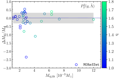
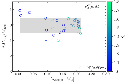
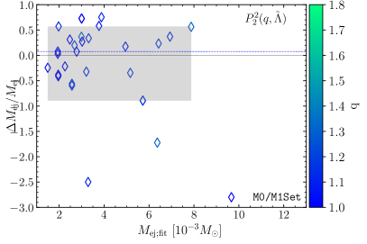
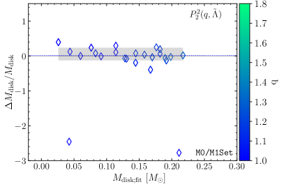
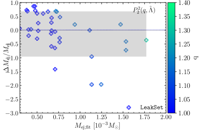
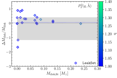
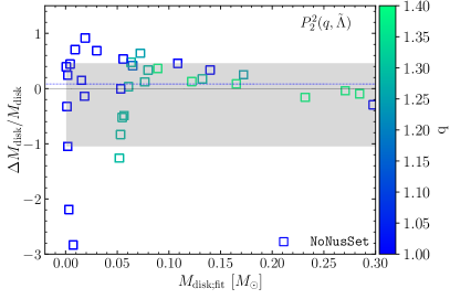
Figure 11: Comparison between the data and values obtained from the fitting formula $P_{2}^{2}(q,\tilde{\Lambda})$ for the ejecta mass (left column of plots) and disk mass (right column of plots). The plot is similar to the 2 and 8, but instead of showing the result for the combined dataset with all models, in each panel only one dataset is used to calibrate the $P_{2}^{2}(q,\tilde{\Lambda})$ fitting formula.

Appendix C Effect of the error measure on the fitting procedure results

In the main text, the comparison between different fitting formulae and their respective calibration is performed using residuals (SSR). Additionally we discuss the $\chi^{2}_{\nu}$ using the error measures found in the literature.

In this appendix we investigate how different error measures and different criteria for fitting procedure affect the result. We focus on the models of M0RefSet only, for which we have errors estimated directly from the numerical relativity (NR) simulations performed at different resolutions (See Table 1 in Nedora et al. (2021)). We also limit the analysis to the $P_{2}^{2}(q,\tilde{\Lambda})$ fitting formula. We consider three approaches: (i) minimizing the residuals, (ii) miminizing the $\chi^{2}_{\nu}$ with the default errors, discussed in the main text and (iii) minimizing $\chi^{2}_{\nu}$ with the NR-informed errors. For the (i) we compute two $\chi^{2}_{\nu}$, computed for both error measures.

For the $M_{\mathrm{e}j}$ we observe that for (i) the $\chi^{2}_{\nu}$ increases by almost $3$ orders of magnitude when employing the NR-informed errors from $1.17$ to $563.92$. Meanwhile, the difference in the quality of the fit computed with minimization of $\chi^{2}_{\nu}$ using these two error measures, i.e., (ii) and (iii), changes only slightly, as Fig. 12 shows. As expected, the extrema of $\Delta M_{\mathrm{e}j}/M_{\mathrm{e}j}$ are the lowest, $(-2.34,0.54)$ when the residuals are minimize. However, even when $\chi^{2}_{\nu}$ is minimized, the increase in extrema is not significant (with respect to the overall fit performance): $(-2.73,0.50)$ for default error measure and $(-2.60,0.51)$ for NR-informed errors.

For the $\langle v_{\infty}\rangle$, we observe no difference between the fit calibrated minimizing residuals (i) or minimizing $\chi^{2}_{\nu}$ with default error (ii), as the error measure is a constant value. However, the increase in $\chi^{2}_{\nu}$ amounts to an order of a magnitude from $0.9$ to $9.3$. When the NR-informed error is used the fit changes slightly at the lower tail of the velocity with the decrease in $\chi^{2}_{\nu}$ to $3.3$.

Similar behaviour is observed for the $\langle Y_{e}\rangle$ and $\langle\theta_{\mathrm{R}MS}\rangle$ as the error measure for these quantities are also constants.

For the $M_{\mathrm{d}isk}$ we observe the similar picture as for the $M_{\mathrm{e}j}$. For (i) the $\chi^{2}_{\nu}$ increases by ${\gtrsim}3$ orders of magnitude from $1.5$ to $192$. However, the difference in the fit quantitative performance with minimization of $\chi^{2}_{\nu}$ using the two error measures, i.e., (ii) and (iii), remains within data points’ error bars (see Fig. 12, left panel).

For a fixed $q=1$ the performance of the $P_{2}^{2}(q,\tilde{\Lambda})$ is shown in Fig. 13. We observe that the largest difference in both cases amounts to $0.25$ in $\log_{10}$ of the respective quantity. The fit computed minimizing the $\chi^{2}_{\nu}$ gives higher values across the considered range of $\tilde{\Lambda}$.

The qualitative behavior of the fits remain, however, unchanged.

That the outcome of the fit calibration depends on the choice of the error measure only when this measure is biased. Otherwise, it is equivalent to minimizing residuals, as is the case for all quantities considered except masses. Regarding the latter, while the qualitative behavior of the fit appears to be independent of the minimization technique, the quantitative difference is present. The error measures considered in the main text are motivated by the finite-resolution errors found in numerical simulations Radice et al. (2018a). However, their use for the statistical analysis of different datasets performed with different physics and numerical setups might not be optimal. This was our motivation to minimize residuals in the fitting formulae analysis in the main text. Employing a more physically and statistically motivated error measure in future analysis, when larger sample of data is available, would lead to better constrained fits.

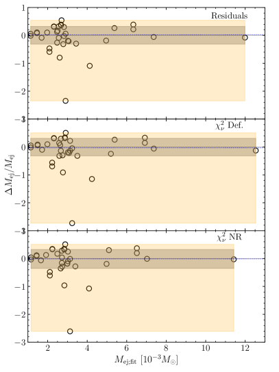
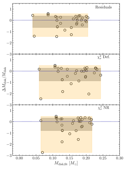
Figure 12: Effects of different calibration methods for $P_{2}^{2}(q,\tilde{\Lambda})$ fit for models of M0RefSet for the ejecta mass (left panel) and disk mass (right panel). We consider the minimization of residuals, $\chi^{2}_{\nu}$ with default error measures (Eqs. (2),(3)), and the errors estimated from multi-resolution analysis in Nedora et al. (2021). Gray / pastel shaded regions mark the $1\sigma\,(68\%)$ / $2\sigma\,(95.4\%)$ confidence intervals.

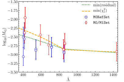
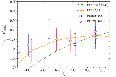
Figure 13: Visual representation of the $P_{2}^{2}(q,\tilde{\Lambda})$ fit for ejecta mass (left panel) and disk mass (right panel). The fits are calibrated with M0/M1Set and M0RefSet, however, only models with $q=1$ are plotted. The fit calibration is done either minimizing residuals or $\chi^{2}_{\nu}$. In the latter case, the default errors are used (and also plotted) namely, Eq. (2) and Eq. (3)

References

- Arcavi et al. (2017) I. Arcavi et al., Nature 551, 64 (2017), arXiv:1710.05843 [astro-ph.HE] .
- Coulter et al. (2017) D. A. Coulter et al., Science (2017), 10.1126/science.aap9811, [Science358,1556(2017)], arXiv:1710.05452 [astro-ph.HE] .
- Drout et al. (2017) M. R. Drout et al., (2017), 10.1126/science.aaq0049, arXiv:1710.05443 [astro-ph.HE] .
- Evans et al. (2017) P. A. Evans et al., (2017), 10.1126/science.aap9580, arXiv:1710.05437 [astro-ph.HE] .
- Hallinan et al. (2017) G. Hallinan et al., (2017), 10.1126/science.aap9855, arXiv:1710.05435 [astro-ph.HE] .
- Kasliwal et al. (2017) M. M. Kasliwal et al., (2017), 10.1126/science.aap9455, arXiv:1710.05436 [astro-ph.HE] .
- Nicholl et al. (2017) M. Nicholl et al., Astrophys. J. 848, L18 (2017), arXiv:1710.05456 [astro-ph.HE] .
- Smartt et al. (2017) S. J. Smartt et al., Nature (2017), 10.1038/nature24303, arXiv:1710.05841 [astro-ph.HE] .
- Soares-Santos et al. (2017) M. Soares-Santos et al. (DES), Astrophys. J. 848, L16 (2017), arXiv:1710.05459 [astro-ph.HE] .
- Tanvir et al. (2017) N. R. Tanvir et al., Astrophys. J. 848, L27 (2017), arXiv:1710.05455 [astro-ph.HE] .
- Troja et al. (2017) E. Troja et al., Nature (2017), 10.1038/nature24290, arXiv:1710.05433 [astro-ph.HE] .
- Mooley et al. (2018) K. P. Mooley, A. T. Deller, O. Gottlieb, E. Nakar, G. Hallinan, S. Bourke, D. A. Frail, A. Horesh, A. Corsi, and K. Hotokezaka, Nature 561, 355 (2018), arXiv:1806.09693 [astro-ph.HE] .
- Ruan et al. (2018) J. J. Ruan, M. Nynka, D. Haggard, V. Kalogera, and P. Evans, Astrophys. J. 853, L4 (2018), arXiv:1712.02809 [astro-ph.HE] .
- Lyman et al. (2018) J. D. Lyman et al., Nat. Astron. 2, 751 (2018), arXiv:1801.02669 [astro-ph.HE] .
- Abbott et al. (2017a) B. P. Abbott et al. (Virgo, LIGO Scientific), Astrophys. J. 850, L39 (2017a), arXiv:1710.05836 [astro-ph.HE] .
- Abbott et al. (2017b) B. P. Abbott et al. (Virgo, LIGO Scientific), Phys. Rev. Lett. 119, 141101 (2017b), arXiv:1709.09660 [gr-qc] .
- Abbott et al. (2019) B. P. Abbott et al. (LIGO Scientific, Virgo), Phys. Rev. X9, 011001 (2019), arXiv:1805.11579 [gr-qc] .
- Abbott et al. (2018) B. P. Abbott et al. (LIGO Scientific, Virgo), (2018), 10.3847/1538-4357/ab0f3d, arXiv:1810.02581 [gr-qc] .
- Lattimer and Schramm (1974) J. M. Lattimer and D. N. Schramm, Astrophys. J. Letters 192, L145 (1974).
- Symbalisty and Schramm (1982) E. Symbalisty and D. N. Schramm, Astrophys. J. Letters 22, 143 (1982).
- Li and Paczynski (1998) L.-X. Li and B. Paczynski, Astrophys.J. 507, L59 (1998), arXiv:astro-ph/9807272 [astro-ph] .
- Kulkarni (2005) S. R. Kulkarni, (2005), arXiv:astro-ph/0510256 [astro-ph] .
- Rosswog et al. (1999) S. Rosswog, M. Liebendoerfer, F. Thielemann, M. Davies, W. Benz, et al., Astron.Astrophys. 341, 499 (1999), arXiv:astro-ph/9811367 [astro-ph] .
- Rosswog (2005) S. Rosswog, Astrophys. J. 634, 1202 (2005), arXiv:astro-ph/0508138 [astro-ph] .
- Metzger et al. (2010) B. Metzger, G. Martinez-Pinedo, S. Darbha, E. Quataert, A. Arcones, et al., Mon.Not.Roy.Astron.Soc. 406, 2650 (2010), arXiv:1001.5029 [astro-ph.HE] .
- Roberts et al. (2011) L. F. Roberts, D. Kasen, W. H. Lee, and E. Ramirez-Ruiz, Astrophys.J. 736, L21 (2011), arXiv:1104.5504 [astro-ph.HE] .
- Kasen et al. (2013) D. Kasen, N. R. Badnell, and J. Barnes, Astrophys. J. 774, 25 (2013), arXiv:1303.5788 [astro-ph.HE] .
- Cowperthwaite et al. (2017) P. S. Cowperthwaite et al., Astrophys. J. 848, L17 (2017), arXiv:1710.05840 [astro-ph.HE] .
- Villar et al. (2017) V. A. Villar et al., Astrophys. J. 851, L21 (2017), arXiv:1710.11576 [astro-ph.HE] .
- Tanaka et al. (2017) M. Tanaka et al., Publ. Astron. Soc. Jap. (2017), 10.1093/pasj/psx121, arXiv:1710.05850 [astro-ph.HE] .
- Perego et al. (2017) A. Perego, D. Radice, and S. Bernuzzi, Astrophys. J. 850, L37 (2017), arXiv:1711.03982 [astro-ph.HE] .
- Kawaguchi et al. (2018) K. Kawaguchi, M. Shibata, and M. Tanaka, Astrophys. J. 865, L21 (2018), arXiv:1806.04088 [astro-ph.HE] .
- Fahlman and Fernández (2018) S. Fahlman and R. Fernández, Astrophys. J. 869, L3 (2018), arXiv:1811.08906 [astro-ph.HE] .
- Nedora et al. (2021) V. Nedora, S. Bernuzzi, D. Radice, B. Daszuta, A. Endrizzi, A. Perego, A. Prakash, M. Safarzadeh, F. Schianchi, and D. Logoteta, Astrophys. J. 906, 98 (2021), arXiv:2008.04333 [astro-ph.HE] .
- Metzger (2020) B. D. Metzger, Living Rev. Rel. 23, 1 (2020), arXiv:1910.01617 [astro-ph.HE] .
- Shibata and Hotokezaka (2019) M. Shibata and K. Hotokezaka, Ann. Rev. Nucl. Part. Sci. 69, 41 (2019), arXiv:1908.02350 [astro-ph.HE] .
- Radice et al. (2020) D. Radice, S. Bernuzzi, and A. Perego, Ann. Rev. Nucl. Part. Sci. 70 (2020), 10.1146/annurev-nucl-013120-114541, arXiv:2002.03863 [astro-ph.HE] .
- Bernuzzi (2020) S. Bernuzzi, Gen. Rel. Grav. 52, 108 (2020), arXiv:2004.06419 [astro-ph.HE] .
- Hotokezaka et al. (2013a) K. Hotokezaka, K. Kiuchi, K. Kyutoku, T. Muranushi, Y.-i. Sekiguchi, et al., Phys.Rev. D88, 044026 (2013a), arXiv:1307.5888 [astro-ph.HE] .
- Bauswein et al. (2013) A. Bauswein, S. Goriely, and H.-T. Janka, Astrophys.J. 773, 78 (2013), arXiv:1302.6530 [astro-ph.SR] .
- Wanajo et al. (2014) S. Wanajo, Y. Sekiguchi, N. Nishimura, K. Kiuchi, K. Kyutoku, and M. Shibata, Astrophys. J. 789, L39 (2014), arXiv:1402.7317 [astro-ph.SR] .
- Sekiguchi et al. (2015) Y. Sekiguchi, K. Kiuchi, K. Kyutoku, and M. Shibata, Phys.Rev. D91, 064059 (2015), arXiv:1502.06660 [astro-ph.HE] .
- Radice et al. (2016) D. Radice, F. Galeazzi, J. Lippuner, L. F. Roberts, C. D. Ott, and L. Rezzolla, Mon. Not. Roy. Astron. Soc. 460, 3255 (2016), arXiv:1601.02426 [astro-ph.HE] .
- Sekiguchi et al. (2016) Y. Sekiguchi, K. Kiuchi, K. Kyutoku, M. Shibata, and K. Taniguchi, Phys. Rev. D93, 124046 (2016), arXiv:1603.01918 [astro-ph.HE] .
- Vincent et al. (2020) T. Vincent, F. Foucart, M. D. Duez, R. Haas, L. E. Kidder, H. P. Pfeiffer, and M. A. Scheel, Phys. Rev. D101, 044053 (2020), arXiv:1908.00655 [gr-qc] .
- Dessart et al. (2009) L. Dessart, C. Ott, A. Burrows, S. Rosswog, and E. Livne, Astrophys.J. 690, 1681 (2009), arXiv:0806.4380 [astro-ph] .
- Fernández et al. (2015) R. Fernández, E. Quataert, J. Schwab, D. Kasen, and S. Rosswog, Mon. Not. Roy. Astron. Soc. 449, 390 (2015), arXiv:1412.5588 [astro-ph.HE] .
- Perego et al. (2014) A. Perego, S. Rosswog, R. Cabezon, O. Korobkin, R. Kaeppeli, et al., Mon.Not.Roy.Astron.Soc. 443, 3134 (2014), arXiv:1405.6730 [astro-ph.HE] .
- Just et al. (2015) O. Just, A. Bauswein, R. A. Pulpillo, S. Goriely, and H. T. Janka, Mon. Not. Roy. Astron. Soc. 448, 541 (2015), arXiv:1406.2687 [astro-ph.SR] .
- Kasen et al. (2015) D. Kasen, R. Fernández, and B. Metzger, Mon. Not. Roy. Astron. Soc. 450, 1777 (2015), arXiv:1411.3726 [astro-ph.HE] .
- Metzger and Fernández (2014) B. D. Metzger and R. Fernández, Mon.Not.Roy.Astron.Soc. 441, 3444 (2014), arXiv:1402.4803 [astro-ph.HE] .
- Martin et al. (2015) D. Martin, A. Perego, A. Arcones, F.-K. Thielemann, O. Korobkin, and S. Rosswog, Astrophys. J. 813, 2 (2015), arXiv:1506.05048 [astro-ph.SR] .
- Wu et al. (2016) M.-R. Wu, R. Fernández, G. Martínez-Pinedo, and B. D. Metzger, Mon. Not. Roy. Astron. Soc. 463, 2323 (2016), arXiv:1607.05290 [astro-ph.HE] .
- Siegel and Metzger (2017) D. M. Siegel and B. D. Metzger, Phys. Rev. Lett. 119, 231102 (2017), arXiv:1705.05473 [astro-ph.HE] .
- Fujibayashi et al. (2018) S. Fujibayashi, K. Kiuchi, N. Nishimura, Y. Sekiguchi, and M. Shibata, Astrophys. J. 860, 64 (2018), arXiv:1711.02093 [astro-ph.HE] .
- Metzger et al. (2018) B. D. Metzger, T. A. Thompson, and E. Quataert, Astrophys. J. 856, 101 (2018), arXiv:1801.04286 [astro-ph.HE] .
- Fernández et al. (2019) R. Fernández, A. Tchekhovskoy, E. Quataert, F. Foucart, and D. Kasen, Mon. Not. Roy. Astron. Soc. 482, 3373 (2019), arXiv:1808.00461 [astro-ph.HE] .
- Miller et al. (2019) J. M. Miller, B. R. Ryan, J. C. Dolence, A. Burrows, C. J. Fontes, C. L. Fryer, O. Korobkin, J. Lippuner, M. R. Mumpower, and R. T. Wollaeger, Phys. Rev. D100, 023008 (2019), arXiv:1905.07477 [astro-ph.HE] .
- Hotokezaka et al. (2013b) K. Hotokezaka, K. Kiuchi, K. Kyutoku, H. Okawa, Y.-i. Sekiguchi, et al., Phys.Rev. D87, 024001 (2013b), arXiv:1212.0905 [astro-ph.HE] .
- Dietrich et al. (2015) T. Dietrich, S. Bernuzzi, M. Ujevic, and B. Brügmann, Phys. Rev. D91, 124041 (2015), arXiv:1504.01266 [gr-qc] .
- Palenzuela et al. (2015) C. Palenzuela, S. L. Liebling, D. Neilsen, L. Lehner, O. L. Caballero, E. O’Connor, and M. Anderson, Phys. Rev. D92, 044045 (2015), arXiv:1505.01607 [gr-qc] .
- Bernuzzi et al. (2016) S. Bernuzzi, D. Radice, C. D. Ott, L. F. Roberts, P. Moesta, and F. Galeazzi, Phys. Rev. D94, 024023 (2016), arXiv:1512.06397 [gr-qc] .
- Lehner et al. (2016) L. Lehner, S. L. Liebling, C. Palenzuela, O. L. Caballero, E. O’Connor, M. Anderson, and D. Neilsen, Class. Quant. Grav. 33, 184002 (2016), arXiv:1603.00501 [gr-qc] .
- Radice et al. (2018a) D. Radice, A. Perego, K. Hotokezaka, S. A. Fromm, S. Bernuzzi, and L. F. Roberts, Astrophys. J. 869, 130 (2018a), arXiv:1809.11161 [astro-ph.HE] .
- Perego et al. (2019) A. Perego, S. Bernuzzi, and D. Radice, Eur. Phys. J. A55, 124 (2019), arXiv:1903.07898 [gr-qc] .
- Kiuchi et al. (2019) K. Kiuchi, K. Kyutoku, M. Shibata, and K. Taniguchi, Astrophys. J. 876, L31 (2019), arXiv:1903.01466 [astro-ph.HE] .
- Endrizzi et al. (2020) A. Endrizzi, A. Perego, F. M. Fabbri, L. Branca, D. Radice, S. Bernuzzi, B. Giacomazzo, F. Pederiva, and A. Lovato, Eur. Phys. J. A 56, 15 (2020), arXiv:1908.04952 [astro-ph.HE] .
- Bernuzzi et al. (2020) S. Bernuzzi et al., Mon. Not. Roy. Astron. Soc. (2020), 10.1093/mnras/staa1860, arXiv:2003.06015 [astro-ph.HE] .
- Dietrich and Ujevic (2017) T. Dietrich and M. Ujevic, Class. Quant. Grav. 34, 105014 (2017), arXiv:1612.03665 [gr-qc] .
- Krüger and Foucart (2020) C. J. Krüger and F. Foucart, Phys. Rev. D 101, 103002 (2020), arXiv:2002.07728 [astro-ph.HE] .
- Radice et al. (2018b) D. Radice, A. Perego, F. Zappa, and S. Bernuzzi, Astrophys. J. 852, L29 (2018b), arXiv:1711.03647 [astro-ph.HE] .
- Coughlin et al. (2019) M. W. Coughlin, T. Dietrich, B. Margalit, and B. D. Metzger, Mon. Not. Roy. Astron. Soc. 489, L91 (2019), arXiv:1812.04803 [astro-ph.HE] .
- Coughlin et al. (2020) M. W. Coughlin, T. Dietrich, S. Antier, M. Almualla, S. Anand, M. Bulla, F. Foucart, N. Guessoum, K. Hotokezaka, V. Kumar, G. Raaijmakers, and S. Nissanke, Mon. Not. Roy. Astron. Soc. 497, 1181 (2020), arXiv:2006.14756 [astro-ph.HE] .
- Bonetti et al. (2019) M. Bonetti, A. Perego, M. Dotti, and G. Cescutti, Mon. Not. Roy. Astron. Soc. 490, 296 (2019), arXiv:1905.12016 [astro-ph.HE] .
- Nedora et al. (2019) V. Nedora, S. Bernuzzi, D. Radice, A. Perego, A. Endrizzi, and N. Ortiz, Astrophys. J. 886, L30 (2019), arXiv:1907.04872 [astro-ph.HE] .
- Nedora et al. (2020) V. Nedora, F. Schianchi, S. Bernuzzi, D. Radice, B. Daszuta, A. Endrizzi, P. Aviral, A. Perego, and F. Zappa, “Mapping dynamical ejecta and disk masses from numerical relativity simulations of neutron star mergers,” (2020).
- Dietrich et al. (2017) T. Dietrich, M. Ujevic, W. Tichy, S. Bernuzzi, and B. Brügmann, Phys. Rev. D95, 024029 (2017), arXiv:1607.06636 [gr-qc] .
- Damour and Nagar (2009) T. Damour and A. Nagar, Phys. Rev. D80, 084035 (2009), arXiv:0906.0096 [gr-qc] .
- Favata (2014) M. Favata, Phys.Rev.Lett. 112, 101101 (2014), arXiv:1310.8288 [gr-qc] .
- Siegel (2019) D. M. Siegel, Eur. Phys. J. A 55, 203 (2019), arXiv:1901.09044 [astro-ph.HE] .
- Foucart et al. (2016a) F. Foucart, E. O’Connor, L. Roberts, L. E. Kidder, H. P. Pfeiffer, and M. A. Scheel, Phys. Rev. D94, 123016 (2016a), arXiv:1607.07450 [astro-ph.HE] .
- Foucart et al. (2018) F. Foucart, M. D. Duez, L. E. Kidder, R. Nguyen, H. P. Pfeiffer, and M. A. Scheel, Phys. Rev. D98, 063007 (2018), arXiv:1806.02349 [astro-ph.HE] .
- Rezzolla and Zanotti (2013) L. Rezzolla and O. Zanotti, Relativistic Hydrodynamics (Oxford University Press, Oxford, 2013).
- Foucart et al. (2016b) F. Foucart, R. Haas, M. D. Duez, E. O’Connor, C. D. Ott, L. Roberts, L. E. Kidder, J. Lippuner, H. P. Pfeiffer, and M. A. Scheel, Phys. Rev. D93, 044019 (2016b), arXiv:1510.06398 [astro-ph.HE] .
- Kawaguchi et al. (2016) K. Kawaguchi, K. Kyutoku, M. Shibata, and M. Tanaka, Astrophys. J. 825, 52 (2016), arXiv:1601.07711 [astro-ph.HE] .