On the accuracy and precision of numerical waveforms: Effect of waveform extraction methodology

Abstract

We present a new set of 95 numerical relativity simulations of non-precessing binary black holes (BBHs). The simulations sample comprehensively both black-hole spins up to spin magnitude of 0.9, and cover mass ratios 1 to 3. The simulations cover on average 24 inspiral orbits, plus merger and ringdown, with low initial orbital eccentricities $e<10^{-4}$. A subset of the simulations extends the coverage of non-spinning BBHs up to mass ratio $q=10$. Gravitational waveforms at asymptotic infinity are computed with two independent techniques: extrapolation and Cauchy characteristic extraction. An error analysis based on noise-weighted inner products is performed. We find that numerical truncation error, error due to gravitational wave extraction, and errors due to the Fourier transformation of signals with finite length of the numerical waveforms are of similar magnitude, with gravitational wave extraction errors dominating at noise-weighted mismatches of $\sim 3\times 10^{-4}$. This set of waveforms will serve to validate and improve aligned-spin waveform models for gravitational wave science.

1 Introduction

The second-generation Advanced Laser Interferometric Gravitational-wave Observatories (LIGO) commenced scientific observation, and are expected to reach their design sensitivity by 2019 [1]. The first direct detection of gravitational waves (GW150914) [2] ushers us into the exciting era of gravitational-wave astronomy. In the coming years, LIGO will be joined by additional gravitational-wave observatories around the world: the Virgo Observatory [3] is expected to begin observations soon, a kilometer-scale interferometric detector is under construction in Japan [4], and a further instrument is planned in India [5].

Coalescing compact object binaries, where each partner can be a black hole or a neutron star, are among the primary science targets of these observatories, and gravitational waves (GWs) from non-eccentric compact object binaries will be searched for with matched filtering [6]. Furthermore, inference of the physical parameters of the source of a GW candidate—like masses and spins—proceeds by comparing the measured gravitational waveform with the theoretically expected waveforms (see e.g. [7]). Therefore, both GW detection and parameter estimation rely on accurate waveform models.

Compact object binaries formed from binary stars are expected to circularize during their GW driven inspiral [8, 9], making it important to model quasi-circular binaries. For stellar-mass binary black holes (BBHs), the sensitivity band of ground-based GW detectors may encompass the last hundreds of orbits, merger and ringdown, depending on the total mass of the binary and the low-frequency sensitivity of the detector. Therefore, full inspiral-merger-ringdown waveform models are needed. Of particular importance are aligned-spin, quasi-circular BBH waveforms, as the recent and planned GW searches employ aligned-spin filter templates [10, 11].

Analytical and numerical modeling of aligned spin BBH systems have been vigorously pursued, resulting in the SEOBNRv1/2 waveform families [12, 13, 14] and the PhenomB/C/D waveform families [15, 16, 17]. Numerical relativity (NR) provides reference waveforms for the late inspiral and merger, against which the analytical waveform models are fitted. Specifically, higher order post-Newtonian coefficients—affecting the inspiral phase—are tuned to improve agreement between the analytical models and NR. Modeling of the plunge and merger is guided entirely by NR, and NR also yields the amplitudes and phasing of the various ringdown modes. The two black holes observed by LIGO in September 2015 were found to be 36 and 29 solar masses [18], with the gravitational wave signal being dominated by the merger part and only about 10 preceeding GW cycles in band [2]. Numerical relativity calibrated waveform models were central to the detection and analyis of this event [2, 18, 19].

The difficulty and high computational cost of performing numerical simulations of BBHs restrict the number of available simulations and the BBH parameters being studied. Difficulty and cost increase both with mass ratio and with the magnitude of the black hole spins. While some simulations push mass-ratio [20] and spin boundaries [21, 22], numerical waveform catalogs most densely cover near equal mass binaries with moderate spin [23, 24, 25, 26, 27].

This paper presents a new set of 95 numerical simulations of non-precessing BBH systems, of which 84 have aligned spins and 11 are non-spinning. The new aligned-spin simulations target low-eccentricity binaries at mass ratios $q\!=\!1,2,3$ and nearly uniformly cover the entire spin-spin plane, up to spin magnitudes of 0.9. The new non-spinning simulations uniformly cover the range of mass ratios up to $q\!=\!10$. These new simulations are comparatively long, and, on average, cover the last 24 orbits of inspiral, merger, and ringdown. This large number of simulated orbits results in a comparatively low initial orbital frequency, so that the simulations cover the Advanced LIGO frequency spectrum  for total masses $M\gtrsim 50M_{\odot}$. In this mass regime, the simulations can be used without additional post-processing steps such as hybridization to post-Newtonian waveforms [24] and the attendant uncertainties arising from post-Newtonian errors [34].

We compute gravitational waveforms at asymptotic infinity with two different methods: with polynomial extrapolation [35, 36, 37] of Regge-Wheeler-Zerilli [38, 39, 40, 41] waveforms extracted at finite radius, and with Cauchy characteristic extraction [42, 43, 44]. Comparison of the resulting asymptotic waveforms allows a study of waveform extraction errors across the parameter space of aligned spin BBHs, extending the study of Ref. [45].

Restricting our analysis to $M\gtrsim 50M_{\odot}$, we analyze numerical truncation error, waveform extraction uncertainties, and the impact of the finite length of the numerical waveforms. When expressed in terms of noise-weighted inner products, the median accuracy of these new numerical waveforms corresponds to overlaps better than 0.9997, i.e., mismatches $<\!3\times 10^{-4}$. The largest contribution to the error budget is uncertainty due to the gravitational-wave extraction method of the NR waveforms. Numerical truncation error and the error in computing noise-weighted inner products of the finite-length waveforms are smaller by a factor of $\sim 2$. The new simulations provide a uniform dataset to validate existing waveform models for aligned spin binaries and to construct improved waveform models.

The remainder of this paper is organized as follows. Section 2 describes the choice of numerical parameters studied here and summarizes our numerical techniques. Section 3 describes our error analysis. We close with a discussion in Sec. 4.

2 Numerical Waveforms

2.1 Choice of parameters

The numerical simulations that we perform consist of 95 different non-precessing configurations. Of these, 11 are non-spinning with mass ratios $q=m_{1}/m_{2}=2.5,\,3.5,\,4.5,\,5.5,\,6.5,\,7,\,7.5,\,8.5,\,9,\,9.5,\,10$, where $m_{i},i=1,2$ denote the individual black hole masses, with $m_{1}$ being the more massive black hole. These mass ratios supplement the existing non-spinning simulations in the SXS waveform catalog [26] to achieve a set of non-spinning waveforms for all mass ratios from $q=1$ to $q=10$ in increments of $\Delta q=0.5$ (see also [46]).

The remaining 84 configurations have $q=1$, 2, or 3, with black hole spins either aligned or anti-aligned with the orbital angular momentum. We parameterize the spin by its projection onto the direction of the orbital angular momentum, i.e.,

$$\chi_{i}:=\frac{\vec{S}_{i}\cdot\hat{L}}{m_{i}^{2}},$$ (1)

where $\vec{S}_{i}$ denotes each hole’s angular momentum vector and $\hat{L}$ the direction of the orbital angular momentum. Our simulations have spin magnitudes as high as $|\chi_{i}|=0.9$. Of these, 22 have only one hole that is spinning, 32 have both holes spinning with equal spin magnitudes, and 30 have both holes spinning with unequal spin magnitudes. For moderate spin magnitudes ($|\chi_{i}|\leq 0.8$ for q=1, and $|\chi_{i}|\leq 0.6$ for $q=2,3$) we use the spin values planned during the NRAR project [27]. We extend this set of configurations with additional runs at spin magnitudes up to 0.9 for equal-mass configurations, and up to 0.85 for mass ratios $q=2$ and $q=3$. The configurations sample various values of the effective spin parameter [47] $\chi_{\rm eff}=S_{\rm eff}/M^{2}$, where

$$\vec{S}_{\rm eff}=\left(1+\frac{75}{113}\frac{m_{2}}{m_{1}}\right)\vec{S}_{1}+\left(1+\frac{75}{113}\frac{m_{1}}{m_{2}}\right)\vec{S}_{2},$$ (2)

and $M=m_{1}+m_{2}$ denotes the total mass. The leading order post-Newtonian spin-contributions to the GW phase and amplitude depend only on $\chi_{\rm eff}$. Past studies [47, 48] found that $\chi_{\rm eff}$ provides a single-spin approximation superior to a mass-weighted average of the two spins. To facilitate future studies on the usefulness of $\chi_{\rm eff}$ for waveform modeling, our set of 95 BBH simulations contains BBH configurations with differing spins, but the same effective spin.

The parameter space coverage of our spinning simulations is shown in Figure 1, where the dashed lines indicate select contours of constant $\chi_{\rm eff}$.

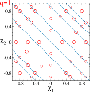
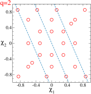
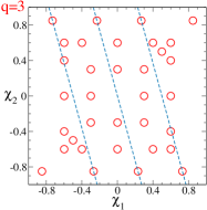
Figure 1: The parameters of the spinning BBH simulations presented here. Mass ratio $q=1$ admits the exchange symmetry $\chi_{1}\leftrightarrow\chi_{2}$; we denote by small circles configurations that are obtained by exploiting this symmetry.

For mass ratios $q=2,3$, $\chi_{1}$ is the spin carried by the more massive black hole. The blue dashed lines indicate select lines of constant $\chi_{\rm eff}$; see equation (2).

2.2 Numerical methods

Our simulations are performed with the Spectral Einstein Code (SpEC) [49]. Quasi-equilibrium initial data are constructed in the extended conformal thin-sandwich formalism [50, 51], using the pseudo-spectral elliptic solver detailed in [52]. For configurations with spins less than $\chi=0.5$, we make the simplifying choices of conformal flatness and maximal slicing. For higher spins, we superpose Kerr-Schild metrics for our free data [53].

For evolutions, we use a computational grid extending from inner excision boundaries, located slightly inside the apparent horizons, to a large outer boundary. We use a first-order representation of the generalized harmonic system [54, 55, 56, 57], with a damped-harmonic gauge condition [58]. The initial orbital eccentricity is reduced to $e\leq 10^{-4}$ with the iterative procedure of [59, 60, 61]. During the evolutions, the pure-outflow excision boundaries are dynamically adjusted to conform to the shapes of the apparent horizons [62, 58, 63]. Interdomain boundary conditions are enforced with a penalty method [64, 65], while constraint-preserving outgoing-wave boundary conditions are imposed at the outer boundary [66, 67, 68]. In addition, the evolution grid is adaptively refined [69] based on the truncation error of each evolved field, the truncation error of the apparent horizon finders, and the local size of constraint violations. After merger, we transition to a grid that only has one excision boundary [62, 63]. Our evolutions here use three resolutions, which we refer to, from low to high, as N3, N4, and N5.

The simulations cover inspiral, merger, and ringdown, with between 18 and 32 inspiral orbits, and an average of 24 orbits.

2.3 Waveform Extraction

Of interest to the gravitational-wave observatories are the asymptotic gravitational waveforms, as they are located $\mathcal{O}(10^{19}\,M)$ from the source binaries. SpEC solves Einstein’s equations on a foliation of spatial hypersurfaces, which extend to the outer boundary of the computational domain. This boundary is typically placed at $\mathcal{O}(10^{3}\,M)$ from the black holes, only a few gravitational wavelengths away from the binary. We apply two distinct techniques to compute the gravitational waveform at asymptotic infinity from the data provided by the Cauchy evolution, namely polynomial extrapolation of gravitational waveforms extracted at finite extraction radii, as well as Cauchy characteristic extraction (CCE). We shall now summarize each of these techniques in turn.

Gravitational wave extrapolation [35, 45] begins with choosing a set of coordinate spheres with radii $\{R_{j}\}$ (typically 24, extending from $\sim 100M$ to near the outer boundary). On these extraction spheres, the following quantities are computed as functions of time: (i) the gravitational wave strain $h_{l,m}$ with the Regge-Wheeler-Zerilli (RWZ) formalism [38, 39, 40, 41]; (ii) the areal radius $R_{ar,j}=\sqrt{A_{j}/4\pi}$, where the surface area of the coordinate sphere $A_{j}$ is computed through integration using the full spatial metric; and (iii) the average of the time-time-component of the space-time metric, $g^{tt}$. A retarded time variable $t_{\mathrm{ret}}$ is constructed as

$$t_{\mathrm{ret}}=t_{\mathrm{corr}}-r_{*},$$ (3)

where

$$\ t_{\mathrm{corr}}=\int_{0}^{t}\mathrm{d}t^{\prime}\sqrt{\frac{-1/g^{tt}}{1-2M_{\mathrm{ADM}}/r_{ar}}},$$ (4)

and

$$r_{*}=r_{ar}+2M_{\mathrm{ADM}}\log\left(\frac{r_{ar}}{2M_{\mathrm{ADM}}}-1\right),$$ (5)

with $M_{\mathrm{ADM}}$ denoting the Arnowitt-Deser-Misner (ADM) mass, which is computed from the initial data set [52]. Since the extrapolation of slowly varying functions is less susceptible to numerical errors in intermediate steps, we extrapolate the complex amplitude $A^{l,m}$ and phase $\phi^{l,m}$ of the spherical harmonic modes $h_{l,m}$, defined as

$$R_{ar,j}Mh_{l,m}(t_{\mathrm{ret}},R_{ar,j})=A^{l,m}(t_{\mathrm{ret}},R_{ar,j})\mathrm{e}^{{\rm i}\phi^{l,m}(t_{\mathrm{ret}},R_{ar,j})}.$$ (6)

Next, we expand the amplitude and phase of all finite radii waveforms in powers of $(\lambda/r_{ar})$ [36], where $\lambda$ is the gravitational wavelength of the $(l=m=2)$ multipole, as

$$A^{l,m}(t_{\mathrm{ret},i},R_{ar,j})=\displaystyle\sum\limits_{k=0}^{n}A^{l,m}_{k}(t_{\mathrm{ret},i},R_{ar,j})\left(\frac{2}{m}\right)^{k}\left(\frac{\lambda}{r_{ar}}\right)^{k},$$ (7)

$$\phi^{l,m}(t_{\mathrm{ret},i},R_{ar,j})=\displaystyle\sum\limits_{k=0}^{n}\phi^{l,m}_{k}(t_{\mathrm{ret},i},R_{ar,j})\left(\frac{2}{m}\right)^{k}\left(\frac{\lambda}{r_{ar}}\right)^{k}.$$ (8)

For the non-oscillatory $m=0$ modes, we extrapolate $h_{l,0}$ directly. The choice of the number of terms to keep before truncating the above expansion, i.e., of $n$, is governed by the gravitational wavelength and truncation error level. If $n$ is too low, crucial higher-order terms will be missed, while if it is too high, over-fitting to noise can lead to diverging polynomials. We examine the errors propagated in the asymptotic waveform due to the truncation of the above expansion in detail for all our simulations in Sec. 3.3.

Having the expansions Eqs. (7) and (8), the $k=0$ terms for both amplitude and phase give the asymptotic GW strain $(r/M)h_{lm}$.

The choices of the radial and time coordinates are important, and are made with the primary consideration of having rapid convergence for the expansion in Eqs. (7) and (8). For a detailed discussion of the various choices made in this procedure, we refer the reader to [35, 45].

A second approach to compute gravitational waveforms at asymptotic infinity is Cauchy characteristic extraction (CCE). This approach solves the full Einstein equations on null hypersurfaces extending from an inner world-tube radius $R_{\Gamma}$ directly to future null infinity $(\mathcal{I}^{+})$. We use the PITTNull characteristic code [42, 43, 70, 71, 72, 44] developed within the Cactus framework [73]. PITTNull solves Einstein’s field equations in the Bondi-Sachs framework [74, 75, 72], in which the metric is given by

$$\mathrm{d}s^{2} = -\left(e^{2\beta}(1+rW)-r^{2}h_{AB}U^{A}U^{B}\right)\mathrm{d}u^{2}$$

$$- 2e^{2\beta}\mathrm{d}u\mathrm{d}r-2r^{2}h_{AB}U^{B}\mathrm{d}u\mathrm{d}y^{A}+r^{2}h_{AB}\mathrm{d}y^{A}\mathrm{d}y^{B},$$

where the retarded time $u=t-r$, $y^{A,B}$ are the two angular coordinates, $\beta$ and $U^{A}$ are the lapse function and shift vector, and $h_{AB}$ is the conformal 2-metric associated with the angular variables. The radial coordinate is compactified to bring $\mathcal{I}^{+}$ into the computational domain. The field equations are written in terms of complex spin-weighted scalar forms of the vector and tensor fields, $J\equiv q^{A}q^{B}h_{AB}$ and $U\equiv q_{A}U^{A}$, where $q^{A}$ is a complex dyad associated with the unit 2-sphere metric that satisfies $q^{A}q_{A}=0$, $q^{A}\bar{q}_{A}=2$, and $q^{A}=\frac{1}{2}(q^{A}\bar{q}^{B}+\bar{q}^{A}q^{B})q_{B}$. An important feature of this formalism is that the field equations can be written as evolution and constraint equations that can be solved one at a time, e.g. see Eq. (2.3)–(2.8) of [76] (which first appeared in [77]). Once we have the field J at the initial null hypersurface $u=u_{0}$, we can integrate Eq. (2.3) of [76] to obtain $\beta$, and subsequently Eq. (2.4)–(2.7) to obtain the other unknowns. Finally, Eq. (2.8) of [76] gives $\partial_{u}J$, which is integrated to obtain $J$ at the next $u=\mathrm{constant}$ null hypersurface.

The initial data for the characteristic evolution is specified on a worldtube $\Gamma$, which is a time succession of spheres of constant coordinate radius $R_{\Gamma}$. A set of outgoing null vectors is constructed on $\Gamma$ to induce the null foliation. The 4-metric data on $\Gamma$ from the Cauchy grid is converted to the null coordinate system by a two step process. First, the 4-metric is converted from a Cartesian to an affine null coordinate system in which the angular metric components are available. Then it is converted to the Bondi characteristic coordinates $(u,r,y^{A},y^{B})$, using the angular metric to get the areal radius $r$. In addition, we also need $J$ on the initial null hypersurface, $u=u_{0}$. For an astrophysical inspiraling binary, this initial data $J$ is determined by the preceding inspiral. Since this inspiral is not known, different choices for estimating $J|_{u=u_{0}}$ can be made [45]. Since the data supplied on the initial null hypersurface does not necessarily agree with that from the Cauchy evolution for $R>R_{\Gamma}$, this leads to an uncertainty that is propagated in the final waveform at $\mathcal{I}^{+}$. By comparing asymptotic waveforms computed at different worldtubes, this uncertainty is measured in Sec. 3.3. At $\mathcal{I}^{+}$, the Bondi News function and the Newman-Penrose scalar are computed and transformed to an inertial frame, from which we obtain gauge invariant waveform multipoles $\Psi_{4}^{l,m}$. We obtain the gravitational wave strain $h_{l,m}$ by a double time-integration of $\Psi_{4}^{l,m}$ using the fixed-frequency integration method of Reisswig & Pollney [78], setting the cut-off frequency used by the algorithm to $\omega_{0}=0.005/M$, i.e. smaller than any physically expected frequency.

Extrapolation and CCE have been carefully compared with each other in Ref. [45] for non-spinning BBHs of mass ratios $q=1$ and $q=6$. We will perform comparisons for aligned spin binaries.

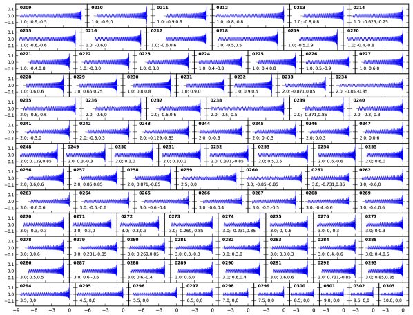
Figure 2: Waveforms computed by CCE plotted as a function of time in units of 1000M. Plotted are gravitational wave strains $rh/M$ emitted in a sky direction in the orbital plane of each simulation. All modes through $l=8$ are summed over, except the non-oscillatory $m=0$ modes. The waveforms are labeled by their SXS catalog numbers in bold, and the BBH parameters ${q,\chi_{1},\chi_{2}}$.

Figure 2 illustrates all the waveforms in the catalog, which will be made publicly available on the SXS website [79]. To highlight features at unequal masses, this figure shows the waveforms emitted in the equatorial plane, summing over all $(l,m)$ modes up to $l=8$, but excluding the non-oscillatory $m=0$ modes because they cannot be reliably integrated to obtain a $h_{l0}$ free of long-term secular drifts.

The waveforms are $5000$–$10000$ M in length, $\sim 20\%$ of which is used up by waveform conditioning steps (described in Sec. 3.1). Due to their finite length, the waveforms will cover the entire detector sensitivity band only when each configuration is above a certain minimum mass $M_{\mathrm{min}}$ [80, 81]. We calculate $M_{\mathrm{min}}$ by imposing the condition that the GW frequency of the $(2,2)$ mode, at the instant where waveform conditioning ends, is $15$ Hz, that is

$$M_{\mathrm{min}}=\frac{c^{3}}{G}\frac{\hat{\Omega}(t_{\mathrm{e}}^{\mathrm{Cond}})}{2\pi}\frac{1}{f_{\mathrm{low}}},$$ (10)

where $t^{\mathrm{e}}_{\mathrm{Cond}}$ is the end time of waveform conditioning window, $\hat{\Omega}=Mf_{\mathrm{GW}}$ is the dimensionless GW frequency, and $f_{\mathrm{low}}=15$ Hz (as discussed in Sec. 3). Therefore, the minimum mass for which we can apply these numerical waveforms directly to Advanced LIGO searches will depend on the details of waveform conditioning procedure. For our preferred middle-long tapering window, the $q\!=\!1$ binaries have $M_{\rm min}$ in the range $[49.6,75.3]M_{\odot}$, the $q\!=\!2$ binaries have $M_{\rm min}\in[51.1,80.9]M_{\odot}$, and the $q\!=\!3$ binaries have $M_{\rm min}\in[58.6,87.9]M_{\odot}$. For the high-mass-ratio systems, $q=3.5\ldots 10$, $M_{\rm min}\in[49.6,127.9]M_{\odot}$. Below, we will analyse total masses $M\in[M_{\rm min},M_{\rm max}]$. We choose $M_{\rm max}$ to be somewhat larger than the largest $M_{\rm min}$, namely $M_{\rm max}=140M_{\odot}$. We note that template based searches are currently performed up to a binary total mass of $100M_{\odot}$ [10]; choosing $M_{\mathrm{max}}=140M_{\odot}$ gives a buffer, should template based searches be used for more massive binaries in the future.

3 Error Analysis

Gravitational-wave searches for compact binaries with Advanced LIGO and Virgo observatories involve matched-filtering detector data using a set (or bank) of modeled waveforms as filter templates. Therefore, the accuracy of filter templates is critical to extracting scientific information from GW observations. In this work, we aim to assess the accuracy of the numerical waveforms shown in Fig. 2 by analyzing different sources of numerical errors. In the absence of knowledge of true waveforms, we vary parameter(s) associated with each of the investigated error sources and use the agreement between corresponding NR waveforms as proxies for their agreement with the true waveforms, i.e. their accuracy.

In the context of matched-filtering searches, the agreement between any two waveforms $h_{1}$ and $h_{2}$ is measured by their noise-weighted overlap $\mathcal{O}$:

$$\mathcal{O}(h_{1},h_{2})=\max_{\phi_{0},t_{0}}\frac{\langle h_{1}(\phi_{0},t_{0}),h_{2}\rangle}{\sqrt{\langle h_{1},h_{1}\rangle\,\langle h_{2},h_{2}\rangle}},$$ (11)

where $\phi_{0}$ and $t_{0}$ are the constant phase and time shifts applied to maximize the agreement between the waveforms, which eliminates the degrees of freedom corresponding to the unknown initial time and phase of the source binary. The inner product $\langle\cdot,\cdot\rangle$, which is the core of the matched-filter, is defined as

$$\langle h_{1},h_{2}\rangle=4\mathrm{Re}\int^{f_{\mathrm{high}}}_{f_{\mathrm{low}}}\frac{\tilde{h}_{1}(f)\tilde{h}_{2}^{*}(f)}{S_{n}(f)}\mathrm{d}f.$$ (12)

Here, $\tilde{h}(f)$ denotes the Fourier transform of the real-valued gravitational waveform $h(t)$, ^∗ denotes complex conjugation, and $S_{n}(f)$ is the one-sided power spectral density of the detector noise. Throughout this paper, we use the zero-detuning high-power (ZERO_DET_HIGH_P) noise curve estimate for Advanced LIGO, and fix the lower frequency cutoff to $f_{\mathrm{low}}=15$ Hz. The upper frequency cutoff is the Nyquist frequency corresponding to the waveform sample rate. Since the waveforms we consider here have frequency content only up to $\sim 1$ kHz, the Nyquist-Shannon sampling theorem says that a sample rate of $2048-4096$ Hz would capture all their physical content. However, a higher sampling rate is needed to control discretization errors when maximizing overlaps over arbitrary time shifts [24]. We employ sampling rates sufficient to ensure that the discretization errors in overlaps stay around $10^{-5}-10^{-4}$. We find $8192$Hz to be sufficient for cases where CCE or EOB waveforms were used, while $16384$ Hz was required for extrapolated waveforms. We also note that we use the dominant $(l,m)=(2,\pm 2)$ multipoles of the gravitational waveform, ignoring the effect of sub-dominant multipoles in this work. Because overlaps tend to cluster near unity, it is often more convenient to use the mismatch between waveforms $\mathcal{M}$ instead, which is defined as

$$\mathcal{M}(h_{1},h_{2})\equiv 1-\mathcal{O}(h_{1},h_{2}).$$ (13)

We now proceed and measure various sources of errors in terms of mismatches.

3.1 Waveform conditioning

Low mass BBH systems spend hundreds of orbits in the LIGO sensitivity band. Therefore, the capability of generating long waveforms is necessary for LIGO detection searches. However, due to the computational expense of numerical relativity, it is difficult to generate long waveforms. While it is possible to generate a small number of very long waveforms [82], the average length of the simulations considered here is approximately 24 orbits to ensure a broad coverage of parameter space.

$\sigma_{\mathrm{start}}$	$t_{1}$	$t_{2}$
start1	$100M$	$500M$
start2	$100M$	$1000M$
start3	$100M$	$2000M$
$\sigma_{\mathrm{end}}$	$t_{3}$	$t_{4}$
end1	$t_{1\%}$	$t_{1\%}+50M$
end2	$t_{10\%}$	$t_{10\%}+100M$

Window	$\sigma_{\mathrm{start}}$	$\sigma_{\mathrm{end}}$
A	start1	end1
B	start2	end1
C	start2	end2
D	start3	end1
E	start3	end2

Table 1: Windowing functions used in this study. The left table gives the different start- and stop-intervals that are utilized, and the right table indicates the combinations of start- and stop-intervals. $M$ is the total mass of the system and $t_{k\%}$ is the time at which the amplitude decays to $k\%$ of its maximum after merger. Figure 3 shows plots of an NR waveform that has been windowed with the combinations given in the right table.

Throughout this study, we only consider total masses large enough such that the numerical waveforms start at a frequency greater than $f_{\rm low}=15$Hz. Nevertheless, there are two sources of noise that contribute to the overall error of the finite-length NR waveforms: First, undesired initial gravitational radiation that is emitted when the initial data relaxes to a steady state [83, 84]. It manifests itself as spurious high-frequency gravitational waves that are emitted during the early numerical evolution, until it relaxes into a quasi-equilibrium state. Second, Gibbs oscillations arise when one Fourier transforms a non-smooth time series, where discontinuous features in the time series (or its derivative) are spread out across a substantial frequency range in the Fourier transform. Furthermore, for numerical simulations, $h(t)$ often tends to a negligibly small, but non-zero value. To mitigate these effects, we apply the Planck-taper window function [85] $\sigma_{T}(t)$ to the waveforms, which tapers both the start and the end of the numerical data. That is, we multiply each numerical waveform $h(t)$ by $\sigma(t)$, where

$$\sigma(t)=\cases{0,&$\quad\;\;\;\,t<t_{1}$,\\ \sigma_{\rm start}(t),&$t_{1}\leq t<t_{2}$,\\ 1,&$t_{2}\leq t<t_{3}$,\\ \sigma_{\rm end}(t),&$t_{3}\leq t<t_{4}$,\\ 0,&$t_{4}\leq t$,\\ }$$ (14)

where $\sigma_{\mathrm{start}}$ is the segment that smoothly increases from 0 to 1 between $t_{1}$ and $t_{2}$, and $\sigma_{\mathrm{end}}$ is the segment that smoothly decreases from 1 to 0 between $t_{3}$ and $t_{4}$:

$$\sigma_{\mathrm{start}}(t) =\left[\exp\left(\frac{t_{2}-t_{1}}{t-t_{1}}+\frac{t_{2}-t_{1}}{t-t_{2}}\right)+1\right]^{-1},$$ (15a)

$$\sigma_{\mathrm{end}}(t) =\left[\exp\left(\frac{t_{3}-t_{4}}{t-t_{3}}+\frac{t_{3}-t_{4}}{t-t_{4}}\right)+1\right]^{-1}.$$ (15b)

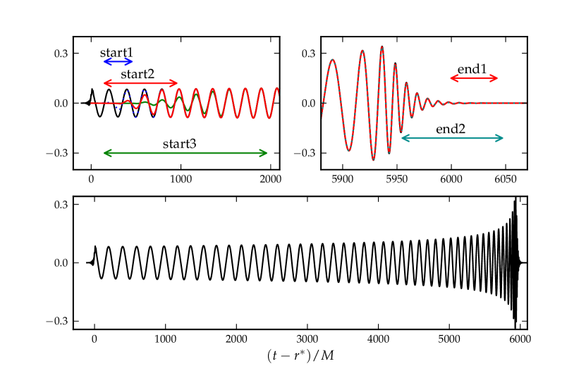
Figure 3: Window function applied to an NR waveform ($q=2$, $\chi_{1}=0.871$, and $\chi_{2}=-0.850$), where the widths of $\sigma_{\mathrm{start}}$ and $\sigma_{\mathrm{end}}$ are given in Table 1. The top left and right panels show the beginning and end of the waveform, respectively, while the bottom panel is the full, unwindowed waveform. The unwindowed waveform is labeled in black, while the coloured lines correspond to the different windowing options as designated by the labeled arrows. The start and end options labeled in red represent the options that are chosen for our preferred window function, B.

We first investigate the impact of Gibbs oscillations on finite-length waveforms in the absence of other numerical errors. For each of the BBH parameters shown in Fig. 1 and for a total mass such that the NR waveform starts at 15 Hz, we construct a long, analytical waveform using the SEOBNRv2 waveform model [12] that has a fixed length of 1000 gravitational-wave cycles. The SEOBNRv2 waveforms can be constructed with negligible computational cost compared to the cost of constructing NR simulations. We manually truncate each one of these long EOB waveforms to the duration of the corresponding NR simulation by discarding the early inspiral. The truncated EOB waveforms now serve as proxies for the finite-length NR waveforms. We subsequently apply tapering windows to the truncated waveforms. We explore five variations of the Planck-taper window function, where we control the width of $\sigma_{\mathrm{start}}$ and $\sigma_{\mathrm{end}}$ by varying $t_{1}$, $t_{2}$, $t_{3}$, and $t_{4}$. Our choices are given in Table 1 and are illustrated in Figure 3.

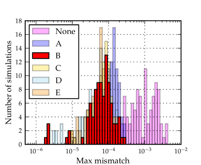
Figure 4: Histogram of maximum mismatches between long, analytic waveforms and finite-length, windowed analytic waveforms. The level of error introduced when finite-length waveforms are used is around 0.2%. Windowed waveforms, however, decrease the error by an order of magnitude. Results strongly indicate that conditioning the waveforms minimizes this length error.

We first determine how closely the truncated EOB waveforms agree with the ‘long’ EOB waveforms. For each configuration, the five truncated, windowed waveforms and the one truncated, non-windowed waveform are compared to the long waveform by computing their mismatches over the mass range $[M_{\mathrm{min}},M_{\mathrm{max}}]$; see equation (10). The maximum mismatch $\mathcal{M}=1-\mathcal{O}(h_{\mathrm{long}},h_{\mathrm{NR\;length,X}})$ is calculated for each window function (out of A–E and non-windowed options), and the procedure is repeated for all configurations.

Results are given in Figure 4. All waveforms considered here start at a frequency below $f_{\rm low}$. Mismatches between non-windowed long and truncated waveforms are between $2\times 10^{-4}$ and $5\times 10^{-3}$ due to spectral leakage of the short waveform’s abrupt turn-on into the sensitivity band $f>f_{\rm low}$, cf. Equation 13. Windowing the truncated waveform reduces the mismatch by almost an order of magnitude. We establish that windowing is important, even for clean data that does not have additional numerical artefacts. For the clean waveforms considered here, it is found that the more aggressive window functions B–E perform better than None or A.

None of our blending functions allows the overlap between the truncated and the long EOB waveform to be larger than $\sim 0.9998$, despite all windowing being applied to the waveform before $f_{\rm low}$, and despite the truncated and the long EOB waveforms being identical after windowing.

Numerical waveforms are short (compared to analytic waveforms) by computational necessity, and below, we will establish that numerical waveform modeling errors result in mismatches $<0.1\%$ when comparing such short waveforms. However, if much longer numerical waveforms are available, Fig. 4 suggests that the current NR waveforms would show mismatches of $\sim 10^{-4}$ relative to the longer ones.

3.2 Numerical truncation error

We begin our error analysis of the numerical simulations by first considering numerical truncation error. The NR simulations are performed at three numerical resolutions (denoted as N3, N4, and N5, with N5 being the highest), and the gravitational waveforms are extracted using either polynomial extrapolation or CCE. To assess numerical truncation error, we fix the GW extraction method, and compare runs at different numerical resolutions.

The NR waveforms are windowed by the five variations of the Planck-taper window function that are described in Table 1. We calculate overlaps as above, comparing waveforms generated at different numerical resolutions, but using the same window function: $\mathcal{O}(h_{i\mathrm{,X}},h_{j\mathrm{,X}})$, for numerical resolutions $i,j=\in\{\mathrm{N3,N4,N5}\}$ and window function X. As before, the mismatches are calculated over a total mass range of $[M_{\mathrm{min}},M_{\mathrm{max}}]$, and the maximum mismatch over the mass range is calculated. For the extrapolation method, we fix the extrapolation order parameter to be $n=3$, and for CCE, we fix the extraction radius to be the outermost radius, as these parameters are determined to yield the most accurate NR waveforms, as discussed in Section 3.3.

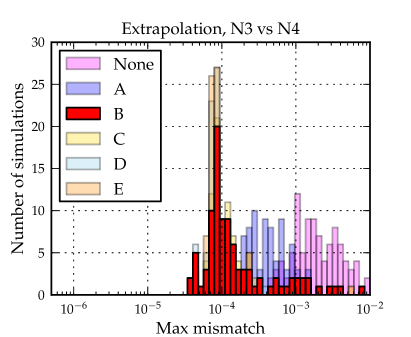
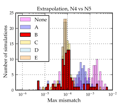
Figure 5: Histograms of mismatches representing numerical truncation error of the extrapolated waveforms. The left panel shows the mass-maximized mismatches between the low and medium numerical resolutions, N3 vs N4, while the right panel shows the maximum mismatches between the medium and high numerical resolutions, N4 vs N5.

Owing to the large number of configurations considered here, the resulting mismatches are histogrammed. Figure 5 shows the numerical truncation error results for extrapolated waveforms. Both the N3 vs N4 and N4 vs N5 comparisons (the left and right panels, respectively) show significantly smaller mismatches when windowing is applied. The window function A uses the short start1 window, cf Fig. 3 and Table 1. Figure 5 illustrates that increasing the length of the start-window to start2 in window function B reduces the overlaps further. Additional lengthening of start2 in window function D, however, does not lead to extra reduction of the mismatch. These findings indicate the presence of substantial resolution-dependent initial transients in the waveforms during the start2 interval, $t\leq 1000M$. These transients have decayed away at the end of the start2 interval, so lengthening to the start3 interval does not affect the mismatch substantially. The end-window does not noticeably impact the mismatches (compare B vs C, or D vs E).

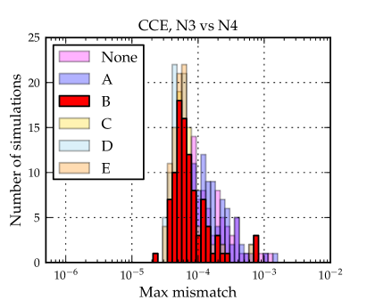
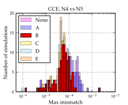
Figure 6: Histograms of the maximum numerical truncation mismatches of the CCE waveforms. The left panel shows the maximum mismatches between the low and medium numerical resolutions, N3 vs N4, while the right panel shows the maximum mismatches between the medium and high numerical resolutions, N4 vs N5.

The numerical truncation error study for the CCE waveforms are repeated, and the results are shown in Figure 6. Comparing Figs. 5 and 6, one notices that the CCE waveforms exhibit lower mismatches than the extrapolated waveforms, in the absence of windowing (None) and for a short start-window (A). Furthermore, the CCE waveforms have fewer outliers at large mismatch than the extrapolated waveforms. These findings can be explained by a smaller amount of high-frequency features in the first $\sim 500M$ of the CCE waveforms. Broadening the window function to B reduces the mismatches of the CCE waveforms to $\sim 10^{-4}$, indicating the presence of initial transients even in the CCE waveforms. Once enough windowing is applied to remove initial transients (window function B or higher), the N3 vs N4 and N4 vs N5 mismatches for CCE and for extrapolated waveforms are similar at $\sim 10^{-4}$. We attribute these residual mismatches of $\sim 10^{-4}$ to genuine differences between the numerical simulations at different resolution (e.g., a difference in the orbital phasing). We therefore conclude that the numerical truncation error corresponds to mismatches of $\sim 10^{-4}$, comparable to the impact of the finite length of the NR waveforms, cf. Fig. 4.

Figures 5 and 6 show clear advantages of a window function at least as invasive as B. The more invasive window functions (C–E) do not exhibit further improvements in Figs. 4–6. Window function B offers therefore the best compromise between needed filtering while leaving the largest portion of the waveforms intact. We will use B throughout the remaining studies in this paper.

3.3 Waveform extraction error

The 3+1 NR simulations presented here have a finite outer boundary radius, and extracted gravitational waves are subject to gauge effects. Moreover, each GW extraction technique has intrinsic parameters that also determine the output: the extrapolation order for GW extrapolation, and the location of the world tube $R_{\Gamma}$ for CCE. Each waveform in our set of simulations is extracted by two different techniques, and we investigate the waveform extraction errors of the extrapolated waveforms and of the CCE waveforms.

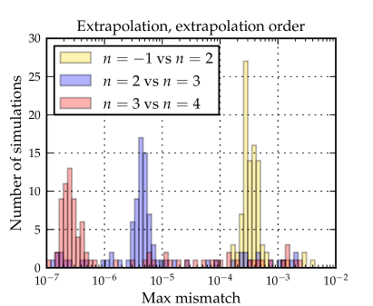
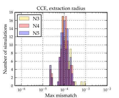
Figure 7: Histogram of maximum mismatches for the intrinsic parameters of each gravitational extraction method. All waveforms were windowed using window function B. Left: Comparison of different GW extrapolation orders $n$ using high-resolution N5 simulations, where $n=-1$ denotes the waveform at the outermost extraction radius without extrapolation. Right: Comparison between CCE waveforms extracted at two different world tubes $R_{\Gamma}$, for all numerical resolutions.

We begin by investigating each GW extraction method separately. For the extrapolation method, the intrinsic parameter is the extrapolation order $n$ in Eqs. 7 and 8. In past studies, it has been found that low $n$ extrapolated waveforms are accurate during the inspiral stage, while high $n$ extrapolated waveforms are accurate during merger [45]. Using the high-resolution (N5) simulations, we extrapolate the RWZ waveforms with different extrapolation order $n$. Windowing each extrapolated waveform with window function B, we compute overlaps between waveforms extrapolated with different order. As before, we compute these overlaps for total mass in the range $[M_{\rm min},M_{\rm max}]$ and take the minimal overlap (i.e. the maximal mismatch). The obtained mismatches are histogrammed and shown in the left panel of Fig. 7. It is found that the errors decrease significantly as the waveforms are extrapolated to higher orders, indicating robust and rapid convergence of the extrapolation procedure with $n$, at least in the integrated sense that is relevant to LIGO. This analysis demonstrates that GW extrapolation converges to a well-determined waveform as $n$ becomes large. However, it is not guaranteed that it converges to a waveform that is correct to within the very small mismatches shown in the left panel of Fig. 7. Assumptions that are common to all extrapolation orders $n$ will influence the extrapolated waveform independent of $n$. Examples of such assumptions are averaging of $g^{tt}$, or the choice of retarded time, cf. Eqs. (3)–(5). The impact of these choices can be estimated through comparison with a different technique to compute asymptotic waveforms, namely, CCE.

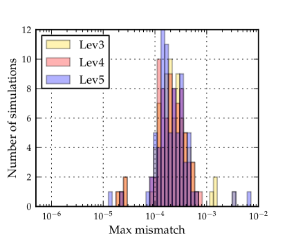
Figure 8: Histogram of overlaps comparing CCE at largest worldtube radius and extrapolation at order $n=3$. Window B is applied to all waveforms, and the different numerical resolutions are denoted by colour. All three numerical resolutions have errors converging at around 0.02%.

CCE also has intrinsic parameters, namely, radius $R_{\Gamma}$ of CCE initial worldtube and the time step of CCE evolution. We performed CCE for two different worldtube radii, $R_{\Gamma}\sim 450M$ and $R_{\Gamma}\sim 350M$ (the precise radii differ for each configuration). For $M_{\rm min}<M<M_{\rm max}$, we compute the mismatches between the resulting CCE waveforms (using window function B), and for each configuration, the largest mismatch in the considered mass range is found. The right panel of Figure 7 shows that the error between the outermost extraction radius and the second outermost extraction radius is $~{}10^{-4}$. The mismatches are independent of the numerical resolution, indicating that the differences between the CCE waveforms obtained at the two different $R_{\Gamma}$ are numerically resolved.

To investigate the importance of the CCE time-step, a few CCE waveforms are computed at smaller CCE time-step. The CCE time-step error is found to be always an order of magnitude smaller than the world-tube radius error shown in the right panel of Fig. 7.

Finally, we compare the two GW extraction methods with each other. We consider NR waveforms, windowed with B, calculated at the highest numerical resolution, N5. The CCE waveforms are calculated from the outermost worldtube, and the extrapolated waveforms are calculated at extrapolation order $n=3$. Figure 8 shows the maximum mismatches between the CCE and extrapolated waveforms for all NR simulations in the set. The mismatches are $\sim 3\times 10^{-4}$ and are larger than the extrapolation-internal and CCE-internal estimates of Fig. 7. The slight increase in mismatches could be caused by systematic effects when the asymptotic waveforms are computed using either technique, and are not captured by the convergence tests of Fig. 7. The mismatches shown in Fig. 8 are independent of the numerical resolution, enforcing our interpretation that the differences are due to systematic effects inside the GW extraction methods. Nevertheless, the degree of similarity between extrapolated and CCE waveforms indicates the high quality of both techniques.

4 Discussion

In this paper, we present a new set of 95 non-precessing binary black hole simulations performed with SpEC. The 84 simulations with spinning black holes explore the $\chi_{1}$–$\chi_{2}$ plane for mass ratios $q=1,2,3$. The remaining 11 non-spinning simulations fill in mass ratios that have not been simulated with SpEC before [61, 26, 62] to achieve a covering of $q\!=\!1$ to $q\!=\!10$ in steps of $0.5$. The simulations cover approximately 24 orbits and have orbital eccentricities of $e\leq 10^{-4}$. All simulations are performed at three different resolutions, and the gravitational wave strain at asymptotic infinity is computed with two complementary methods, extrapolation [35, 36, 37] of Regge-Wheeler-Zerilli waveforms [38, 39, 40, 41] extracted at finite radii, and Cauchy characteristic extraction (CCE)  [42, 43, 44, 45].

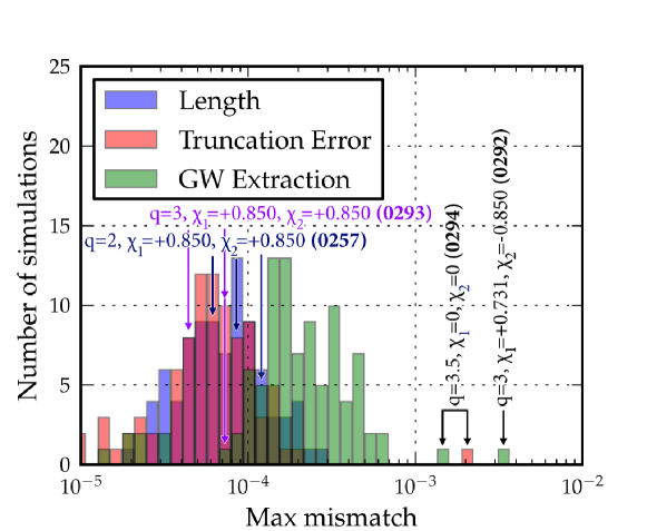
Figure 9: Summary of the main results. Error due to gravitational wave extraction method is slightly dominant over other numerical errors. Labeled are the outliers and BBH systems with large black-hole spins, with their SXS catalog numbers in bold.

Advanced LIGO is searching for gravitational waves of aligned-spin BBH systems during its early observing runs. For BBHs in particular, the late-inspiral, merger and ringdown phases comprise a major portion of the detectable signal [33]. Semi-analytic models of aligned-spin BBHs have been vigorously developed during the past years, resulting in the SEOBNR models [13, 12] and phenomenological models PhenomB/C/D [15, 16, 17]. These models are broadly based on extensions of the perturbative post-Newtonian theory, and extensively rely on fully general-relativistic numerical simulations of BBHs for calibration. The new numerical waveforms presented here cover the spin-spin space for both aligned and anti-aligned systems up to dimensionless spins of $0.9$. These new waveforms can serve to independently validate existing search templates (which have been calibrated only in a subset of the parameter space populated by the new simulations) to investigate systematic effects relevant to parameter estimation [7] and to calibrate improved waveform models. In addition, the parameters estimated GW150914 are encompassed in this new set of numerical waveforms [18].

To aid these tasks, we perform an error analysis of the new waveforms in terms of noise-weighted inner products, as appropriate for data-analysis applications. The following sources of error are considered: (a) the finite length and numerical artifacts in the early part of the NR waveforms, which cause spectral leakage and additional high-frequency features when transformed to the frequency domain; (b) numerical truncation error; and (c) errors from GW extraction, i.e. details of the procedure used to compute asymptotic waveforms from the Cauchy evolution. To ensure that the waveforms always cover the entire Advanced LIGO frequency spectrum, we perform our error analysis for a total mass range $[M_{\rm min},M_{\rm max}]$. $M_{\rm min}$ is determined independently for each NR simulation such that, even for the most intrusive windowing considered, the usable part of the NR waveform covers all frequencies above the low-frequency cutoff $f_{\rm low}$. We choose $M_{\rm max}=140M_{\odot}$, and $f_{\rm low}=15$Hz .

To estimate the impact of the finite length of the NR waveforms, we generate a set of long, analytic waveforms and truncate them to lengths comparable to the NR waveforms. Within the mass range $[M_{\rm min},M_{\rm max}]$ (i.e. at masses such that the truncated waveforms start below $f_{\rm low}$), we compute overlaps between long and truncated waveforms, and find mismatches of $\sim 2\times 10^{-3}$. When windowing the truncated waveforms (such that the window ends below $f_{\rm low}$), these mismatches drop to $\sim 2\times 10^{-4}$. This value is interpreted as a lower limit of how well inner products involving finite-length waveforms can be evaluated.

Each simulation is performed at three resolutions, denoted as N3, N4, and N5. The numerical truncation error is analyzed by calculating the mismatches between waveforms at different numerical resolutions. The mismatches substantially decrease from no windowing, over to a small start-window A, and then to a medium-duration start-window B, but no further decrease of mismatch is found when the start-window is lengthened to D. Details of different windowing configurations can be found in Sec. 3.1. The reduction in mismatch is substantially stronger than the finite-length waveform test based on analytical waveforms, indicating that the NR waveforms have unphysical radiation content during the first $\sim 1000M$ of the evolution, arising from the relaxation of the initial data to a quasi-equilibrium state [83]. When window function B is applied, those numerical artifacts are removed, and the residual mismatches of $\sim 0.01\%$ correspond to the numerical truncation error. We note that the mismatch computed between low and medium resolution (N3 vs N4), and between medium and high numerical resolution (N4 vs N5) is comparable, cf. the left and right panels of Figs. 5 and 6. This lack of clear convergence might arise from the use of adaptive-mesh-refinement [69], which causes resolution changes at different times for the different resolutions. The numerical truncation error mismatches are smaller than the GW extraction errors shown in Fig. 8, and therefore, are not the dominant source of waveform uncertainty.

Finally, we studied the errors arising from GW extraction and computation of the asymptotic waveforms at future null infinity. Extrapolation of finite-radius RWZ strain converges uniformly with extrapolation order $n$, cf. Fig. 7. However, extrapolation seems to be susceptible to features in the data arising from different numerical resolution, which is indicated by the tail of outliers with mismatch $\gtrsim 0.03\%$ in Fig. 5. In contrast, for CCE waveforms, the outliers at large mismatch are absent in Fig. 8, indicating that CCE more robustly generates similar asymptotic waveforms in the presence of numerical truncation error. Unfortunately, the CCE waveforms show a stronger dependence on the radius of the CCE worldtube $R_{\Gamma}$, as seen in the right panel of Fig. 7. The CCE errors in the right panel of Fig. 7 are independent of numerical resolution (N3 vs N4 vs N5) of the underlying Cauchy evolution. This implies that the mismatches shown in this figure are actually dominated by the choice of CCE worldtube, and indeed, the impact of numerical truncation error is smaller by a factor of $\sim 2$, cf. Fig. 6.

The three principal sources of error—finite length, truncation error, and GW extraction error—are summarized and contrasted with each other in Figure 9. The three sources of error are comparable in magnitude, with GW extraction error, measured as the difference between CCE and extrapolated waveforms, being slightly more dominant. The second largest source of error arises from numerical truncation, and finite length is smallest of these three error sources.

As summarized by Fig. 9, we expect the windowed NR waveforms presented here to agree with the true, infinitely long inspiral waveform to a mismatch better than $0.02\%$ for the considered mass range $[M_{\rm min},M_{\rm max}]$ when evaluated for Advanced LIGO design sensitivity. To place this into context, we note that detection template banks are usually constructed to accept a fitting factor of 0.97 or a mismatch of $3\%$ between templates and possible signals. Our NR waveforms are significantly more accurate, and as a result, they can be used to validate waveform models for BBH detection searches. A conservative accuracy requirement for parameter estimation is given in Ref. [87]: the waveform model is sufficiently accurate for parameter estimation on a signal with signal-to-noise ratio $\rho$ if the waveform uncertainty $\delta h$ satisfies

$$\frac{\langle\delta h,\delta h\rangle}{\langle h,h\rangle}<\frac{1}{\rho^{2}}.$$ (15p)

By Taylor-expansion, one can show that $1-{\cal O}(h,h+\delta h)=\frac{\langle\delta h,\delta h\rangle}{2\langle h,h\rangle}$. Therefore, Eq. (15p) implies that waveform errors $\delta h$ should be irrelevant for parameter estimation of signals that satisfy

$$1-{\cal O}(h,h+\delta h)<\frac{1}{2\rho^{2}}.$$ (15q)

That means that a mismatch of $3\times 10^{-4}$ is acceptable for signals with SNRs $\rho\lesssim 40$.

To substantially improve the uncertainty of the numerical waveforms, one would have to improve on all three sources of error considered here. The numerical simulations would have to be longer to mitigate the finite-length errors. Alternatively, one would have to mitigate the impact of the abrupt turn-on of the finite-length waveforms to a better degree than possible with windowing. One strategy for doing so is the construction of hybrid waveforms [24, 25], where a post-Newtonian inspiral waveform is smoothly attached to the first few clean GW cycles of the NR waveform. Truncation error can be addressed by using higher numerical resolution. It is less clear how to improve the GW extraction error; presumably, CCE errors decay with CCE worldtube radius $R_{\Gamma}$, so a larger radius $R_{\Gamma}$ might reduce the CCE uncertainties. Alternatively, one can consider using Cauchy characteristic matching, where information from the characteristic code is injected back into the 3+1 Cauchy evolution through the outer boundary. All of these solutions require an increase in computational cost and the wall-clock time to perform the simulations and GW extraction.

References

- [1] Aasi J et al. (LIGO Scientific Collaboration) 2015 Class. Quantum Grav. 32 074001 (Preprint 1411.4547)
- [2] Abbott B P et al. (Virgo, LIGO Scientific) 2016 Phys. Rev. Lett. 116 061102 (Preprint 1602.03837)
- [3] Acernese F, Agathos M, Agatsuma K, Aisa D, Allemandou N, Allocca A, Amarni J, Astone P, Balestri G, Ballardin G, Barone F, Baronick J P, Barsuglia M, Basti A, Basti F, Bauer T S, Bavigadda V, Bejger M, Beker M G, Belczynski C, Bersanetti D, Bertolini A, Bitossi M, Bizouard M A, Bloemen S, Blom M, Boer M, Bogaert G, Bondi D, Bondu F, Bonelli L, Bonnand R, Boschi V, Bosi L, Bouedo T, Bradaschia C, Branchesi M, Briant T, Brillet A, Brisson V, Bulik T, Bulten H J, Buskulic D, Buy C, Cagnoli G, Calloni E, Campeggi C, Canuel B, Carbognani F, Cavalier F, Cavalieri R, Cella G, Cesarini E, Chassande-Mottin E, Chincarini A, Chiummo A, Chua S, Cleva F, Coccia E, Cohadon P F, Colla A, Colombini M, Conte A, Coulon J P, Cuoco E, Dalmaz A, D’Antonio S, Dattilo V, Davier M, Day R, Debreczeni G, Degallaix J, Deléglise S, Pozzo W D, Dereli H, Rosa R D, Fiore L D, Lieto A D, Virgilio A D, Doets M, Dolique V, Drago M, Ducrot M, Endrőczi G, Fafone V, Farinon S, Ferrante I, Ferrini F, Fidecaro F, Fiori I, Flaminio R, Fournier J D, Franco S, Frasca S, Frasconi F, Gammaitoni L, Garufi F, Gaspard M, Gatto A, Gemme G, Gendre B, Genin E, Gennai A, Ghosh S, Giacobone L, Giazotto A, Gouaty R, Granata M, Greco G, Groot P, Guidi G M, Harms J, Heidmann A, Heitmann H, Hello P, Hemming G, Hennes E, Hofman D, Jaranowski P, Jonker R J G, Kasprzack M, Kéfélian F, Kowalska I, Kraan M, Królak A, Kutynia A, Lazzaro C, Leonardi M, Leroy N, Letendre N, Li T G F, Lieunard B, Lorenzini M, Loriette V, Losurdo G, Magazzù C, Majorana E, Maksimovic I, Malvezzi V, Man N, Mangano V, Mantovani M, Marchesoni F, Marion F, Marque J, Martelli F, Martellini L, Masserot A, Meacher D, Meidam J, Mezzani F, Michel C, Milano L, Minenkov Y, Moggi A, Mohan M, Montani M, Morgado N, Mours B, Mul F, Nagy M F, Nardecchia I, Naticchioni L, Nelemans G, Neri I, Neri M, Nocera F, Pacaud E, Palomba C, Paoletti F, Paoli A, Pasqualetti A, Passaquieti R, Passuello D, Perciballi M, Petit S, Pichot M, Piergiovanni F, Pillant G, Piluso A, Pinard L, Poggiani R, Prijatelj M, Prodi G A, Punturo M, Puppo P, Rabeling D S, Rácz I, Rapagnani P, Razzano M, Re V, Regimbau T, Ricci F, Robinet F, Rocchi A, Rolland L, Romano R, Rosińska D, Ruggi P, Saracco E, Sassolas B, Schimmel F, Sentenac D, Sequino V, Shah S, Siellez K, Straniero N, Swinkels B, Tacca M, Tonelli M, Travasso F, Turconi M, Vajente G, van Bakel N, van Beuzekom M, van den Brand J F J, Broeck C V D, van der Sluys M V, van Heijningen J, Vasúth M, Vedovato G, Veitch J, Verkindt D, Vetrano F, Viceré A, Vinet J Y, Visser G, Vocca H, Ward R, Was M, Wei L W, Yvert M, żny A Z and Zendri J P (VIRGO) 2015 Class. Quantum Grav. 32 024001 (Preprint 1408.3978)
- [4] Aso Y, Michimura Y, Somiya K, Ando M, Miyakawa O, Sekiguchi T, Tatsumi D and Yamamoto H (The KAGRA Collaboration) 2013 Phys. Rev. D 88(4) 043007 (Preprint 1306.6747) URL http://link.aps.org/doi/10.1103/PhysRevD.88.043007
- [5] Unnikrishnan C S 2013 International Journal of Modern Physics D 22 1341010
- [6] Finn L S 1992 Phys. Rev. D 46 5236
- [7] Veitch J, Raymond V, Farr B, Farr W, Graff P, Vitale S, Aylott B, Blackburn K, Christensen N, Coughlin M, Del Pozzo W, Feroz F, Gair J, Haster C J, Kalogera V, Littenberg T, Mandel I, O’Shaughnessy R, Pitkin M, Rodriguez C, Röver C, Sidery T, Smith R, Van Der Sluys M, Vecchio A, Vousden W and Wade L 2015 Phys. Rev. D 91(4) 042003 URL http://link.aps.org/doi/10.1103/PhysRevD.91.042003
- [8] Peters P C and Mathews J 1963 Phys. Rev. 131 435–440 URL http://link.aps.org/abstract/PR/v131/p435
- [9] Peters P C 1964 Phys. Rev. 136 B1224–B1232 URL http://link.aps.org/abstract/PR/v136/pB1224
- [10] Abbott B P et al. (LIGO Scientific Collaboration, Virgo Collaboration) 2016 Submitted to to PRD (Preprint 1602.03839)
- [11] Usman S A et al. 2015 (Preprint 1508.02357)
- [12] Taracchini A, Buonanno A, Pan Y, Hinderer T, Boyle M, Hemberger D A, Kidder L E, Lovelace G, Mroue A H, Pfeiffer H P, Scheel M A, Szilagyi B, Taylor N W and Zenginoglu A 2014 Phys. Rev. D 89 (R) 061502 (Preprint 1311.2544)
- [13] Taracchini A, Pan Y, Buonanno A, Barausse E, Boyle M, Chu T, Lovelace G, Pfeiffer H P and Scheel M A 2012 Phys. Rev. D 86 024011 (Preprint 1202.0790)
- [14] Pan Y, Buonanno A, Buchman L T, Chu T, Kidder L E, Pfeiffer H P and Scheel M A 2010 Phys. Rev. D 81 084041 (Preprint 0912.3466)
- [15] Ajith P, Hannam M, Husa S, Chen Y, Bruegmann B, Dorband N, Mueller D, Ohme F, Pollney D, Reisswig C, Santamaria L and Seiler J 2011 Phys. Rev. Lett. 106 241101 (Preprint 0909.2867)
- [16] Santamaría L, Ohme F, Ajith P, Brügmann B, Dorband N, Hannam M, Husa S, Mösta P, Pollney D, Reisswig C, Robinson E L, Seiler J and Krishnan B 2010 Phys. Rev. D 82 064016 (Preprint 1005.3306)
- [17] Khan S, Husa S, Hannam M, Ohme F, Pürrer M, Forteza X J and Bohé A 2015 (Preprint 1508.07253)
- [18] Abbott B P et al. (LIGO Scientific Collaboration, Virgo Collaboration) 2016 (Preprint 1602.03840)
- [19] Abbott B P et al. (LIGO Scientific Collaboration, Virgo Collaboration) 2016 (Preprint 1602.03841)
- [20] Lousto C O and Zlochower Y 2011 Phys. Rev. Lett. 106(4) 041101 URL http://link.aps.org/doi/10.1103/PhysRevLett.106.041101
- [21] Lovelace G et al. 2015 Class. Quantum Grav. 32 065007 (Preprint 1411.7297)
- [22] Scheel M A, Giesler M, Hemberger D A, Lovelace G, Kuper K, Boyle M, Szilágyi B and Kidder L E 2015 Class. Quantum Grav. 32 105009 (Preprint 1412.1803)
- [23] Aylott B, Baker J G, Boggs W D, Boyle M, Brady P R et al. 2009 Class. Quantum Grav. 26 165008 (Preprint 0901.4399)
- [24] Ajith P, Boyle M, Brown D A, Brugmann B, Buchman L T et al. 2012 Class. Quantum Grav. 29 124001
- [25] Ajith P, Boyle M, Brown D A, Brugmann B, Buchman L T et al. 2013 Class. Quantum Grav. 30 199401 URL http://stacks.iop.org/0264-9381/29/i=12/a=124001
- [26] Mroue A H, Scheel M A, Szilagyi B, Pfeiffer H P, Boyle M, Hemberger D A, Kidder L E, Lovelace G, Ossokine S, Taylor N W, Zenginoglu A, Buchman L T, Chu T, Foley E, Giesler M, Owen R and Teukolsky S A 2013 Phys. Rev. Lett. 111 241104 (Preprint 1304.6077)
- [27] Hinder I et al. (The NRAR Collaboration) 2014 Class. Quantum Grav. 31 025012 (Preprint 1307.5307)
- [28] Waldman S J 2011 The advanced ligo gravitational wave detector Tech. Rep. LIGO-P0900115-v2 LIGO Project
- [29] Harry I, Nitz A, Brown D A, Lundgren A, Ochsner E et al. 2014 Phys. Rev. D 89 024010 (Preprint 1307.3562)
- [30] Ajith P, Fotopoulos N, Privitera S, Neunzert A and Weinstein A J 2014 Phys. Rev. D 89 084041 (Preprint 1210.6666)
- [31] Brown D A, Harry I, Lundgren A and Nitz A H 2012 Phys. Rev. D 86 084017 (Preprint 1207.6406)
- [32] Nitz A H, Lundgren A, Brown D A, Ochsner E, Keppel D and Harry I W 2013 ArXiv:1307.1757 (Preprint 1307.1757)
- [33] Brown D A, Kumar P and Nitz A H 2013 Phys. Rev. D 87 082004 (Preprint 1211.6184)
- [34] MacDonald I, Mroué A H, Pfeiffer H P, Boyle M, Kidder L E, Scheel M A, Szilágyi B and Taylor N W 2013 Phys. Rev. D 87 024009 (Preprint 1210.3007)
- [35] Boyle M and Mroué A H 2009 Phys. Rev. D 80 124045–14 (Preprint 0905.3177) URL http://link.aps.org/abstract/PRD/v80/e124045
- [36] Boyle M O 2008 Accurate gravitational waveforms from binary black-hole systems Ph.D. thesis California Institute of Technology URL http://etd.caltech.edu/etd/available/etd-01122009-143851/
- [37] Boyle M 2013 Phys. Rev. D 87 104006 URL http://link.aps.org/doi/10.1103/PhysRevD.87.104006
- [38] Regge T and Wheeler J A 1957 Phys. Rev. 108 1063–1069
- [39] Zerilli F J 1970 Phys. Rev. Lett. 24 737–738
- [40] Sarbach O and Tiglio M 2001 Phys. Rev. D 64 084016 URL http://link.aps.org/abstract/PRD/v64/e084016
- [41] Rinne O, Buchman L T, Scheel M A and Pfeiffer H P 2009 Class. Quantum Grav. 26 075009
- [42] Bishop N T, Gómez R, Lehner L and Winicour J 1996 Phys. Rev. D 54 6153–6165 (Preprint 0706.1319) URL http://link.aps.org/abstract/PRD/v54/p6153
- [43] Bishop N T, Gómez R, Isaacson R A, Lehner L, Szilágyi B and Winicour J 1998 Cauchy-characteristic matching Black Holes, Gravitational Radiation and the Universe ed Iyer B R and Bhawal B (Dordrecht: Kluwer) chap 24 (Preprint gr-qc/9801070)
- [44] Babiuc M C, Szilágyi B, Winicour J and Zlochower Y 2011 Phys. Rev. D 84(4) 044057 (Preprint 1011.4223) URL http://link.aps.org/doi/10.1103/PhysRevD.84.044057
- [45] Taylor N W, Boyle M, Reisswig C, Scheel M A, Chu T, Kidder L E and Szilágyi B 2013 Phys. Rev. D 88(12) 124010 (Preprint 1309.3605) URL http://link.aps.org/doi/10.1103/PhysRevD.88.124010
- [46] Blackman J, Field S E, Galley C R, Szilágyi B, Scheel M A, Tiglio M and Hemberger D A 2015 Phys. Rev. Lett. 115 121102 (Preprint 1502.07758)
- [47] Ajith P 2011 Phys. Rev. D 84 084037 (Preprint 1107.1267)
- [48] Pürrer M, Hannam M, Ajith P and Husa S 2013 Phys. Rev. D 88 064007 (Preprint 1306.2320)
- [49] http://www.black-holes.org/SpEC.html
- [50] Yo H J, Cook J N, Shapiro S L and Baumgarte T W 2004 Phys. Rev. D 70 084033 erratum: [PhysRevD.70.089904]
- [51] Cook G B and Pfeiffer H P 2004 Phys. Rev. D 70 104016
- [52] Pfeiffer H P, Kidder L E, Scheel M A and Teukolsky S A 2003 Comput. Phys. Commun. 152 253–273 (Preprint gr-qc/0202096)
- [53] Lovelace G, Owen R, Pfeiffer H P and Chu T 2008 Phys. Rev. D 78 084017
- [54] Friedrich H 1985 Commun. Math. Phys. 100 525–543 URL http://www.springerlink.com/content/w602g633428x8365
- [55] Garfinkle D 2002 Phys. Rev. D 65 044029
- [56] Pretorius F 2005 Class. Quantum Grav. 22 425–451 URL http://stacks.iop.org/0264-9381/22/425
- [57] Lindblom L, Scheel M A, Kidder L E, Owen R and Rinne O 2006 Class. Quantum Grav. 23 S447–S462 (Preprint gr-qc/0512093v3)
- [58] Szilágyi B, Lindblom L and Scheel M A 2009 Phys. Rev. D 80 124010 (Preprint 0909.3557)
- [59] Mroué A H and Pfeiffer H P 2012 (Preprint 1210.2958)
- [60] Buonanno A, Kidder L E, Mroué A H, Pfeiffer H P and Taracchini A 2011 Phys. Rev. D 83 104034 (Preprint 1012.1549)
- [61] Buchman L T, Pfeiffer H P, Scheel M A and Szilágyi B 2012 Phys. Rev. D 86 084033 (Preprint 1206.3015)
- [62] M A Scheel, M Boyle, T Chu, L E Kidder, K D Matthews and H P Pfeiffer 2009 Phys. Rev. D 79 024003 (Preprint arXiv:gr-qc/0810.1767)
- [63] Hemberger D A, Scheel M A, Kidder L E, Szilágyi B, Lovelace G, Taylor N W and Teukolsky S A 2013 Class. Quantum Grav. 30 115001 (Preprint 1211.6079) URL http://stacks.iop.org/0264-9381/30/i=11/a=115001
- [64] Gottlieb D and Hesthaven J S 2001 J. Comput. Appl. Math. 128 83–131 ISSN 0377-0427 URL http://dx.doi.org/10.1016/S0377-0427(00)00510-0
- [65] Hesthaven J S 2000 Appl. Num. Math. 33 23–41
- [66] Lindblom L, Scheel M A, Kidder L E, Owen R and Rinne O 2006 Class. Quantum Grav. 23 447 (Preprint gr-qc/0512093)
- [67] Rinne O 2006 Class. Quantum Grav. 23 6275–6300 URL http://stacks.iop.org/0264-9381/23/6275
- [68] Rinne O, Lindblom L and Scheel M A 2007 Class. Quantum Grav. 24 4053–4078 URL http://stacks.iop.org/0264-9381/24/4053
- [69] Szilágyi B 2014 Int. J. Mod. Phys. D 23 1430014 (Preprint 1405.3693)
- [70] Babiuc M C, Bishop N T, Szilágyi B and Winicour J 2009 Phys. Rev. D 79 084011 (Preprint 0808.0861)
- [71] Bishop N T, Gomez R, Lehner L, Maharaj M and Winicour J 1997 Phys. Rev. D56 6298–6309 (Preprint qr-qc/9708065)
- [72] Winicour J 1998 Living Rev. Rel. 1 5 (Preprint gr-qc/0102085)
- [73] The Cactus Computational Toolkit http://www.cactuscode.org
- [74] Bondi H, van der Burg M G J and Metzner A W K 1962 Proc. R. Soc. Lond. A 269 21–52
- [75] Sachs R K 1962 Proc. R. Soc. Lond. A 270 103–126 ISSN 00804630 URL http://www.jstor.org/stable/2416200
- [76] Handmer C J, Szilágyi B and Winicour J (Preprint 1502.06987)
- [77] Winicour J 1983 J. Math. Phys. 1193
- [78] Reisswig C and Pollney D 2011 Class. Quantum Grav. 28 195015 (Preprint 1006.1632)
- [79] http://www.black-holes.org/waveforms
- [80] Harry G M (LIGO Scientific Collaboration) 2010 Class. Quantum Grav. 27 084006
- [81] Shoemaker D (LIGO Collaboration) 2010 Advanced LIGO anticipated sensitivity curves LIGO Document T0900288-v3 URL https://dcc.ligo.org/cgi-bin/DocDB/ShowDocument?docid=2974
- [82] Szilagyi B, Blackman J, Buonanno A, Taracchini A, Pfeiffer H P et al. 2015 Phys. Rev. Lett. 115 031102 (Preprint 1502.04953)
- [83] Lovelace G 2009 Class. Quantum Grav. 26 114002
- [84] Sperhake U, Brügmann B, Gonzalez J, Hannam M and Husa S 2007 Head-on collisions of different initial data Proceedings of the eleventh Marcel Grossmann Meeting (Preprint 0705.2035v1)
- [85] McKechan D, Robinson C and Sathyaprakash B 2010 Class. Quantum Grav. 27 084020 (Preprint 1003.2939)
- [86] Boyle M 2016 Phys. Rev. D 93(8) 084031 URL http://link.aps.org/doi/10.1103/PhysRevD.93.084031
- [87] Lindblom L, Owen B J and Brown D A 2008 Phys. Rev. D 78 124020 (Preprint 0809.3844)
- [88] Loken C, Gruner D, Groer L, Peltier R, Bunn N, Craig M, Henriques T, Dempsey J, Yu C H, Chen J, Dursi L J, Chong J, Northrup S, Pinto J, Knecht N and Zon R V 2010 J. Phys.: Conf. Ser. 256 012026