Effective interpretations of a diphoton excess

Abstract

We discuss some consistency tests that must be passed for a successful explanation of a diphoton excess at larger mass scales, generated by a scalar or pseudoscalar state, possibly of a composite nature, decaying to two photons. Scalar states at mass scales above the electroweak scale decaying significantly into photon final states generically lead to modifications of Standard Model Higgs phenomenology. We characterise this effect using the formalism of Effective Field Theory (EFT) and study the modification of the effective couplings to photons and gluons of the Higgs. The modification of Higgs phenomenology comes about in a variety of ways. For scalar $0^{+}$ states, a component of the Higgs and the heavy boson can mix. Lower energy phenomenology gives a limit on the mixing angle, which gets generated at one loop in any theory explaining the diphoton excess. Even if the mixing angle is set to zero, we demonstrate that a relation exists between lower energy Higgs data and a massive scalar decaying to diphoton final states. If the new boson is a pseudoscalar, we note that if it is composite, it is generic to have an excited scalar partner that can mix with a component of the Higgs, which has a stronger coupling to photons. In the case of a pseudoscalar, we also characterize how lower energy Higgs phenomenology is directly modified using EFT, even without assuming a scalar partner of the pseudoscalar state. We find that naturalness concerns can be accommodated, and that pseudoscalar models are more protected from lower energy constraints.

1 Introduction

The global data set reported by LEP, the Tevatron, LHC and a host of low-energy experiments is consistent with the Standard Model (SM) of particle physics. With the discovery of a $0^{+}$ scalar ($h$) consistent in its properties with the scalar $0^{+}$ component of the SM Higgs doublet ($H$), any extension of the SM that aims to explain new phenomena is constrained by an even larger bevy of lower energy tests. With the initial reporting of run II data at $\sqrt{s}\cong 13\,{\rm TeV}$, lower energy tests now include the properties of the "Higgs pole" measurements, fixed to $m_{h}\cong 125\,{\rm GeV}$, measured at $\sqrt{s}\cong 7,8\,{\rm TeV}$ in run I. In this paper, we discuss a set of consistency conditions for scalars with mass scales $m_{s}\gg m_{h}$ that generate a significant decay to diphoton final states, arising from these lower energy measurements. We will assume that the 125 GeV scalar is approximately the SM Higgs boson and study the perturbation of its properties using the Standard Model Effective Field Theory (SMEFT) formalism. The modification of the SM Higgs properties comes about in a variety of ways. For example, a component of the SM Higgs can mix with a new $0^{+}$ scalar or higher-mass resonances. The constraints we derive on the mixing from the experimentally established Higgs couplings must be respected by any models with new scalars that can mix significantly with the Higgs. Other constraints, not directly tied to mixing, are also present when studying low-energy phenomenology. We characterize these matching effects using the SMEFT.

Our motivation is the report of a slight excess of diphoton events in the ATLAS and CMS data ATLAS-CONF-2015-081 ; CMS-PAS-EXO-15-004 at $\sim 750$ GeV. This excess might be, and arguably most likely is, a statistical fluctuation ATLAS-CONF-2015-081 ; CMS-PAS-EXO-15-004 ; LEE . However, the possibility that this excess is generated by new physics has received a lot of attention. Many authors have considered models in which the hypothesized scalar is composite, due to the need for it to couple to gluons or photons despite it being neutral. It is interesting to consider what effects such a state could have on the observed properties of the Higgs boson. Mixing of $h$ with any new states that decay to diphotons will introduce a shift in the expected branching ratio for $h\to\gamma\gamma$. With the measurements of run I, it is known that any such perturbation cannot greatly alter the observed branching ratio, which is $B(h\to\gamma\gamma)\cong 2\times 10^{-3}$. Numerous higher dimensional operators at lower scales have also been probed at LHC in run I, and in Electroweak Precision Data (EWPD) studies. We study the consequences of a diphoton excess at $\sim 750$ GeV in a wide class of models arising from consistency with these lower energy tests.

The purpose of this paper is to further develop these consistency tests and to apply them to generic models that could explain the putative excess. Although some of the constraints we will derive can be satisfied by choosing parameters such that the scalar-h mixing angle is sufficiently small in some models, it is interesting to ask whether such values are natural or if they require fine tuning. This issue is sharpened by the fact that the mixing of interest is necessarily generated by the same operators that are assumed to exist for the purpose of explaining the diphoton events. Other (weaker) constraints we derive are not related to the scalar-h mixing angle at all, but still must be respected.

On the other hand, pseudoscalar states are forbidden by parity from mixing with $h$. However, we will argue that pseudoscalar states in the spectrum of a strongly confining sector are likely to be accompanied by scalar states, with an even stronger (effective) coupling to photons, on fairly general grounds, leading to indirect constraints on sectors with composite pseudoscalars as the lightest states. Further, we characterize how pseudoscalar states still lead to modified properties of the SM Higgs in lower energy experiments using the formalism of the SMEFT. The conditions we develop provide a challenge to the construction of consistent strongly interacting models for the diphoton excess.

1.1 Properties of the diphoton excess at $\sim 750{\rm GeV}$

The properties of the $\sim 750$ $\rm GeV$ diphoton excess have been reported in detail by the experimental collaborations ATLAS-CONF-2015-081 ; CMS-PAS-EXO-15-004 . In brief summary, the excess at $\sim 750$ $\rm GeV$ in diphoton final states is characterised as resonant production with an approximate cross section $\sigma(pp\rightarrow S\rightarrow\gamma\,\gamma)\approx 8[fb]$. The excess in ATLAS data has a local statistical significance of $3.6\,\sigma$ and global significance of $2.0\,\sigma$, while that of CMS is at $2.6\,\sigma$, with a global significance of only $1.2\,\sigma$. The two experiments have differing preferences for the width of the resonance, with CMS preferring a narrow state relative to the experimental resolution of about 6 GeV, while the ATLAS data prefer a larger width of around $45\,{\rm GeV}$. For this reason we will formulate our consistency conditions in a manner that allows the width to be easily adjusted, to a future experimental value, that is more consistent between the experimental results.

2 Scalar models

The Landau-Yang theorem Landau:1948kw ; Yang:1950rg states that a resonance decaying to diphotons can only have spin 0 or spin 2. Here we do not consider spin 2 models, or the simultaneous production of other, undetected, states to consider other possibilities. Spin zero particles can be either scalar or pseudoscalar, and either fundamental or composite. We first focus on the scalar case.

In a fairly general class of models, the scalar field $S$ couples to gluons, photons and possibly quarks in order to explain the production and decay of $S$ into photons that give the diphoton excess. For a scalar of mass $m_{s}$ and width $\Gamma_{s}$, one can express the extra (due to $S$) contribution to the cross section times branching ratio to photons as

$$\Delta\sigma(pp\rightarrow S\rightarrow\gamma\,\gamma) = \frac{\Gamma(S\rightarrow\gamma\,\gamma)}{m_{s}\,\Gamma_{s}\,s}\left[\mathcal{C}_{gg}\,\Gamma(S\rightarrow gg)+\mathcal{C}_{\gamma\,\gamma}\,\Gamma(S\rightarrow\gamma\,\gamma)+\sum_{q}\,\mathcal{C}_{q}\,\Gamma(S\rightarrow q\,\bar{q})\right].$$ (1)

$$= 2.3{\rm\,pb}\times\frac{\Gamma(S\rightarrow\gamma\,\gamma)}{m_{s}}\sum_{i}{\cal C}_{i}\,{\rm Br}(S\to i\,i)$$

For $\sqrt{s}=13\,{\rm TeV}$ the dimensionless coefficients are approximately

$$\mathcal{C}_{i}=\{\mathcal{C}_{\gamma\gamma},\mathcal{C}_{b},\mathcal{C}_{c},\mathcal{C}_{s},\mathcal{C}_{u},\mathcal{C}_{d},\mathcal{C}_{gg}\}\simeq\{0.53,15.3,35.7,83,1054,627,2137\}.$$ (2)

For example if $\Gamma(s\rightarrow\gamma\,\gamma)\sim\Gamma(s\rightarrow gg)\sim 0.01\,m_{s}$, we find $\sigma\sim[fb]\times\mathcal{C}_{i}$. The $\cal{C}_{\gamma\gamma}$ term was recently derived in Csaki:2015vek using the equivalent photon approximation, assuming that the inverse of the impact parameter scaled to the proton radius is $r_{\star}\sim 0.13$. The latter coefficients were generated in Ref. Franceschini:2015kwy at a renormalization scale $\mu=m_{s}$ using MSTW2008 parton distribution functions (PDFs) Martin:2009iq . The parton luminosities are such that gluonic or photonic production of the state can dominate. Utilizing the quark production mechanism has been examined in Ref. Aloni:2015mxa , and found to be challenging.

We focus on the cases of production and decay through $gg\rightarrow S$ and $S\rightarrow\gamma\,\gamma$. We consider the case where the scalar field $S$ couples via the operators

$$\mathcal{L}_{int}=\frac{c_{G}\,g_{3}^{2}}{\Lambda_{g}}S\,G^{\mu\,\nu}\,G_{\mu\,\nu}+\frac{c_{B}\,g_{1}^{2}}{\Lambda_{\gamma}}S\,B^{\mu\,\nu}\,B_{\mu\,\nu}+\frac{c_{W}\,g_{2}^{2}}{\Lambda_{\gamma,2}}S\,W^{\mu\,\nu}\,W_{\mu\,\nu}.$$ (3)

Note that some notation is reused here from the SMEFT operator basis. Decays through the latter operator lead to enhanced couplings to $W^{+}W^{-}$, $ZZ$ and $Z\,\gamma$ final states, while the first two yield smaller levels of such decays. Decays to $Z\gamma$ are disfavoured by correlated searches at the mass scale $\sim 750\,{\rm GeV}$. Ref Aad:2014fha reports a $95\%$ C.L. bound on $\sigma(pp\rightarrow S\rightarrow Z(\ell^{+}\,\ell^{-})\,\gamma)$ of $\lesssim 0.3\,{\rm fb}$, whereas the expected deviation associated with the $\gamma\gamma$ excess, assuming the decay is generated by the coupling to $\rm SU(2)_{L}$ (and the $Z$ and decaying to $\ell^{+}\,\ell^{-}$), is $\sim 2\,\rm{fb}$. It is possible to tune away this tension by having both the operators $O_{B}$ and $O_{W}$ present with correlated Wilson coefficients Harigaya:2015ezk (implicitly defined in Eqn.3); however we will not further consider generating $c_{W}$ since $Z\gamma$ bounds are not the essential point of this study. The decay widths are related to the remaining dimension-five operators, introduced with the given normalization, as

$$\Gamma(S\rightarrow\gamma\,\gamma)=\frac{4\,\pi\,\alpha_{ew}^{2}\,m_{s}^{3}}{\Lambda_{\gamma}^{2}}\,c_{B}^{2},\quad\Gamma(S\rightarrow gg)=\frac{32\,\pi\,\alpha_{s}^{2}\,m_{s}^{3}}{\Lambda_{g}^{2}}\,c_{G}^{2}.$$ (4)

Using (4), we can rewrite the cross section for the diphoton excess (1) as

$$\frac{\Delta\sigma(pp\rightarrow\gamma\,\gamma)}{8[fb]}\left(\frac{\Gamma_{s}}{45\,{\rm GeV}}\right)\cong 6546\,\left(\frac{m_{s}^{2}\,c_{B}^{2}}{\Lambda_{\gamma}^{2}}\right)\,\left[\left(\frac{m_{s}^{2}\,c_{G}^{2}}{\Lambda_{g}^{2}}\right)+2.4\times 10^{-7}\,\left(\frac{m_{s}^{2}\,c_{B}^{2}}{\Lambda_{\gamma}^{2}}\right)\right].$$ (5)

The gauge couplings $\alpha_{s},\alpha_{ew}$ are evaluated at the scale $m_{s}\cong 750\,{\rm GeV}$. We note that, in the presence of the operators generated by integrating out the scalar $S$ at its mass, the running of $\alpha_{s},\alpha_{ew}$ is modified Jenkins:2013zja . The corresponding Wilson coefficients in the SMEFT can receive contributions from other unknown UV physics. Such nonresonant contributions are neglected. We also note that the running effect on the production and decay of the scalar particle is higher order in the power counting, and neglected. We run $\alpha_{s},\alpha_{ew}$ up from the scale $m_{Z}$ using SM relations, so that $\alpha_{s}(750\,{\rm GeV})\cong 0.09,$ and $\alpha_{ew}(750\,{\rm GeV})\cong 1/126.5$.

In a valid EFT expansion, one expects that $m_{s}<\Lambda_{\gamma,g}$. If we normalized the Wilson coefficients proportional to a loop factor $\sim(16\pi)^{-2}$ in the case of some weakly coupled renormalizable UV models, large Wilson coefficients are required. Extreme solutions where $c_{B}/\Lambda_{\gamma}\ll c_{G}/\Lambda_{g}$ or $c_{B}/\Lambda_{\gamma}\gg c_{G}/\Lambda_{g}$ are possible. One naturally expects $\Lambda_{g}\sim\Lambda_{\gamma}$ and $c_{B}$ and $c_{G}$ to differ only by group theory factors, in scenarios where a common mediator generates the two decays.

2.1 Integrating out $S$

Minimal scalar field models have the potential Lagrangian terms

$$\mathcal{L}_{V} = -\lambda_{SM}\left(H^{\dagger}H-\frac{1}{2}v^{2}\right)^{2}-\frac{m_{s}^{2}}{2}\,S^{2}+\frac{\kappa}{4!}\,S^{4}+\,\lambda\,\Lambda_{c}\,S\,H^{\dagger}H+\lambda_{2}\,\Lambda_{c}\,S^{3}+\lambda_{3}\,S^{2}\,(H^{\dagger}H)+\cdots$$

No unbroken discrete symmetry exists that forbids the $\lambda,\lambda_{2}$ terms, since $S$ decays. Here $\Lambda_{c}$ is the cutoff scale of the toy model effective Lagrangian, and we assume that some unknown states with a mass scale $\sim\Lambda_{c}$ generate the coupling of $S$ to photons and gluons. Due to the presence of effective dimension five terms in the Lagrangian, higher order terms are also generated in the potential suppressed by $1/\Lambda_{c}$. Since $m_{s}\gg v$, it is interesting to consider the case that $S$ decays through manifestly $\rm SU(3)\times SU(2)_{L}\times U(1)_{Y}$ invariant operators. Integrating out $S$ one obtains the effective lagrangian suitable for describing Higgs-gauge boson couplings,

$$\mathcal{L}=\mathcal{L}_{SM}+\frac{C_{HG}(m_{s})\,g_{3}^{2}}{\Lambda^{2}}H^{\dagger}\,H\,G^{\mu\,\nu}\,G_{\mu\,\nu}+\frac{C_{HB}(m_{s})\,g_{1}^{2}}{\Lambda^{2}}H^{\dagger}\,H\,B^{\mu\,\nu}\,B_{\mu\,\nu},$$ (6)

where

$$\frac{C_{HG}(m_{s})}{\Lambda^{2}}=\frac{c_{G}\,\lambda}{m_{s}^{2}}\,\frac{\Lambda_{c}}{\Lambda_{g}},\quad\frac{C_{HB}(m_{s})}{\Lambda^{2}}=\frac{c_{B}\,\lambda}{m_{s}^{2}}\,\frac{\Lambda_{c}}{\Lambda_{\gamma}}.$$ (7)

At lower scales $\mu$, the Wilson coefficients are then, in a leading log approximation, (only retaining the Yukawa couplings $Y_{t},Y_{b}$) Jenkins:2013zja ; Jenkins:2013wua ; Alonso:2013hga ; Alonso:2014zka

$$C_{HG}(\mu) = \left(1-\log\left[\frac{{m_{s}}}{\mu}\right]\,\frac{12\,\lambda+2\,N_{c}\,((\sqrt{2}M_{t})^{2}+(\sqrt{2}M_{b})^{2})/v^{2}-6\,g_{1}^{2}y_{h}^{2}-9\,g_{2}^{2}/2}{16\pi^{2}}\right)C_{HG}(m_{s}),$$

$$C_{HB}(\mu) = \left(1-\log\left[\frac{{m_{s}}}{\mu}\right]\,\frac{12\,\lambda+2\,N_{c}\,((\sqrt{2}M_{t})^{2}+(\sqrt{2}M_{b})^{2})/v^{2}+2y_{h}^{2}g_{1}^{2}-9\,g_{2}^{2}/2}{16\pi^{2}}\right)C_{HB}(m_{s}),$$

$$C_{uH}(\mu) = -\frac{\sqrt{2}M_{t}}{v}\,\frac{2\,g_{3}^{4}}{\pi^{2}}\,\log\left[\frac{{m_{s}}}{\mu}\right]\,C_{HG}(m_{s})-\frac{\sqrt{2}M_{t}}{v}\frac{3(y_{h}^{2}+2y_{q}y_{u})}{4\pi^{2}}g_{1}^{4}\log\left[\frac{{m_{s}}}{\mu}\right]C_{HB}(m_{s}),$$

$$C_{dH}(\mu) = -\frac{\sqrt{2}M_{b}}{v}\,\frac{2\,g_{3}^{4}}{\pi^{2}}\,\log\left[\frac{{m_{s}}}{\mu}\right]\,C_{HG}(m_{s})-\frac{\sqrt{2}M_{b}}{v}\frac{3(y_{h}^{2}+2y_{q}y_{d})}{4\pi^{2}}g_{1}^{4}\log\left[\frac{{m_{s}}}{\mu}\right]C_{HB}(m_{s}),$$

$$C_{uG}(\mu) = \frac{\sqrt{2}M_{t}}{4\,\pi^{2}\,v}g_{3}^{3}\,\log\left[\frac{{m_{s}}}{\mu}\right]C_{HG}(m_{s}),$$

$$C_{uB}(\mu) = \frac{\sqrt{2}M_{t}}{16\,\pi^{2}\,v}(2g_{1}^{3}\,(y_{q}+y_{u}))\,\log\left[\frac{{m_{s}}}{\mu}\right]\,C_{HB}(m_{s}),$$

$$C_{dG}(\mu) = \frac{\sqrt{2}M_{b}}{4\,\pi^{2}\,v}g_{3}^{3}\,\,\log\left[\frac{{m_{s}}}{\mu}\right]\,C_{HG}(m_{s}),$$

$$C_{dB}(\mu) = \frac{\sqrt{2}M_{b}}{16\,\pi^{2}\,v}(2g_{1}^{3}\,(y_{q}+y_{d}))\,\log\left[\frac{{m_{s}}}{\mu}\right]\,C_{HB}(m_{s}),$$

$$C_{HWB}(\mu) = -\frac{4g_{1}^{3}g_{2}y_{h}}{16\pi^{2}}\log\left[\frac{{m_{s}}}{\mu}\right]C_{HB}(m_{s}),$$ (8)

with $y_{h}=1/2,y_{q}=1/6,y_{u}=2/3,y_{d}=-1/3$ being the hypercharges of the indicated particles. Here the $O_{uH},O_{dH},O_{eH},O_{uG}$, $O_{dG},O_{uB}$, $O_{dB},O_{HWB},O_{H}$ operators are defined as in Ref.Grzadkowski:2010es . The Higgs potential is also changed in a nontrivial fashion

$$\delta\lambda_{SM}(\mu) = -\frac{3m_{h}^{2}}{4\pi^{2}}\,g_{1}^{4}\,y_{h}^{2}\,\log\left[\frac{{m_{s}}}{\mu}\right]\,C_{HB}(m_{s}),$$ (9)

$$C_{H}(\mu) = -\frac{3}{\pi^{2}}\,\lambda\left(g_{1}^{4}\,y_{h}^{2}\right)\,\log\left[\frac{{m_{s}}}{\mu}\right]\,C_{HB}(m_{s})+\left(\frac{3}{\pi^{2}}g_{1}^{6}\,y_{h}^{4}+\frac{3}{4\,\pi^{2}}g_{1}^{4}\,g_{2}^{2}\,y_{h}^{2}\right)\,\log\left[\frac{{m_{s}}}{\mu}\right]\,C_{HB}(m_{s}).$$

Here $\delta\lambda_{SM}$ is the modification of the running of the Higgs self-coupling relative to how it runs in the SM, below the scale $m_{s}$. It is interesting to note that these one-loop effects would have a nontrivial implication for the running and shape of the potential, if the diphoton excess was substantiated. We will resist drawing conclusions about the fate of the universe due to this observation. The modified potential will redefine the effective Higgs vacuum expectation value, but in an unobservable fashion in current experiments. For the particular case of Higgs physics, to get a sense of the impact on lower energy phenomenology, we note

$$C_{HG}(m_{h}) \cong 0.94\,C_{HG}(m_{s}),$$ (10)

$$C_{HB}(m_{h}) \cong 0.94\,C_{HB}(m_{s}),$$ (11)

$$C_{uH}(m_{h}) \cong -0.46\,C_{HG}(m_{s})-0.0011\,C_{HB}(m_{s}),$$ (12)

$$C_{dH}(m_{h}) \cong -0.011\,C_{HG}(m_{s})-7.85\times 10^{-6}\,C_{HB}(m_{s}),$$ (13)

$$C_{uG}(m_{h}) \cong 0.054\,C_{HG}(m_{s}),$$ (14)

$$C_{dG}(m_{h}) \cong 0.0013\,C_{HG}(m_{s}),$$ (15)

$$C_{uB}(m_{h}) \cong 8.8\times 10^{-4}\,C_{HB}(m_{s}),$$ (16)

$$C_{dB}(m_{h}) \cong -4.4\times 10^{-6}\,C_{HB}(m_{s}),$$ (17)

$$C_{HWB}(m_{h}) \cong -6.9\times 10^{-4}\,C_{HB}(m_{s}).$$ (18)

Flavour indices have been suppressed, due to the scenario considered. There is a (up-down quark) flavour non-universal effect. Note the large effect on the top Yukawa coupling at the low scale. The (assumed) SM Higgs field at 125 GeV coupling to the top gets modified as

$$\kappa_{t}-1=\frac{v^{2}}{\sqrt{2}\,\Lambda^{2}}\left(0.46\,C_{HG}(m_{s})+0.0011\,C_{HB}(m_{s})\right).$$ (19)

Similarly one finds a modification for the coupling of the $h\,Z\,Z$ interaction of the form

$$(0.94s_{\theta}^{2})\,\sqrt{2}\,v\,h\,Z^{\mu\,\nu}\,Z_{\mu\,\nu}\,C_{HB}(m_{s})$$ (20)

with $s_{\theta}^{2}$ referring to the Weinberg angle. The correction to the angle due to $C_{HWB}$ for this term is higher order. This correction leads to an effective modification of $\kappa_{Z}$. Taking into account the typical offshellness in the decays $h\rightarrow Z\,Z^{\star}$ into fermion final states Contino:2013kra , one finds

$$\kappa_{Z}-1\cong 0.2\,\frac{m_{w}^{2}}{\Lambda^{2}}C_{HB}(m_{s}).$$ (21)

The effects on $\kappa_{Z}$, $\kappa_{t}$ are in general subdominant in the minimal scenario considered and can be neglected. In general, a scalar singlet of the form considered above is well isolated from inducing large low-energy effects.

As states of mass scale $\Lambda_{c}$ generate the $c_{B}$ operator at the scale $\Lambda_{\gamma}$, it is necessary that they are charged under $U(1)_{Y}$. One expects a large number of operators to be generated at the scale $\Lambda_{c}$, with contributions to operators that include SM states that are charged under $U(1)_{Y}$, at least at the two-loop level. In this case, the detailed impact on low-energy phenomenology can differ from the minimal case sketched here. When the Wilson coefficient of $S\,H^{\dagger}\,H$ is suppressed, two-loop effects can be comparable, or dominant, over the effects that we study in detail. One also expects one-loop contributions to the operators $O_{HG},O_{HB}$ on general grounds. Our analysis assumes that such direct matching contributions are small enough to be neglected. The couplings of the states that generate $C_{G,B}$ to the SM Higgs are unknown and can be small.

2.2 Generating the $S\,H^{\dagger}\,H$ operator

On general grounds one expects the coupling of the scalar state to be sizable with $H^{\dagger}\,H$, and for the scalar to have a sizable self-coupling term $S^{3}$. These operators are relevant. Of course, pure naturalness expectations for scalar sectors are under pressure due to the measured Higgs mass. Assuming $\lambda\,\Lambda_{c}\sim[\rm TeV]$ the induced Higgs mass value is not strongly perturbed as $\Delta m_{h}^{2}\sim[\rm TeV]^{2}/8\pi^{2}$, so considering separations of scales where $\lambda\,\Lambda_{c}>m_{s}$ by an order one factor does not introduce significant extra tuning to the Higgs sector.

As we will characterize in more detail below, the scenario where $\lambda\,\lambda_{c}$ is a value proximate to the cutoff scale, is problematic. At scales below $m_{s}$, the presence of the $S\,H^{\dagger}\,H$ operator leads to the higher dimensional operators $O_{HB},O_{HG}$ in the SMEFT. If it is assumed that $\lambda\,\lambda_{c}$ is somehow suppressed, or fixed to zero, quantum corrections regenerate this mixing due to the interactions assumed above, to explain the excess in Eqn.3. The mixing between $S$ and $h$ due to $c_{B}$ is generated by the one-loop diagram shown in Fig.1 a. This gives a Naive Dimensional Analysis (NDA) Manohar:1983md estimate of the coefficient of $S\,H^{\dagger}\,H$ of the form

$$\lambda\,\Lambda_{c}\gtrsim\frac{g_{1}^{4}\,m_{s}^{2}}{32\,\pi^{2}}\,\frac{c_{B}(m_{s})}{\Lambda_{\gamma}},$$ (22)

when the bare and loop induced terms of the Wilson coefficient of the operator $SH^{\dagger}\,H$ are not canceled against one another, at the scale $\mu=m_{s}$.

Figure 1: Diagrams generating the mixing of $S$ and $H$ at one loop due to the couplings required for $gg\rightarrow S$ and $S\rightarrow\gamma\,\gamma$, illustrated with the insertion of a box.

The generation of $S\,H^{\dagger}\,H$ due to $c_{G}$ is a two-loop effect. A typical diagram is given in Fig.1 b. The divergence in the diagram leading to the mixing is approximately

$$\sim{\rm Tr}\left[T_{A}T_{A}\right]y_{t}^{2}g_{3}^{2}\frac{m_{s}^{2}\,c_{G}}{(16\pi^{2})^{2}\epsilon\Lambda_{g}},$$ (23)

in dimensional regularization in $d=4-2\epsilon$ dimensions. The colour factors enhance the magnitude of the diagram, as expected. The $\epsilon$ poles cancel in the matching onto the lower energy theory. However, we utilize the corresponding finite terms generated from the logarithmic dependence linked to the divergence in this diagram as an NDA-inspired estimate of the size of the Wilson coefficient of the $SH^{\dagger}\,H$ operator. We give the exact result for the pole of the sum of the diagrams of this form in the Appendix.

2.3 Direct matching contributions to the $O_{HB}$, $O_{HG}$ operators

There are also other direct one-loop contributions to the Wilson coefficients of the SMEFT operators shown in Fig.2 a,b. Fig.2 a depends on an unknown scalar coupling in the potential – $\lambda_{3}$, but does not require the operator $SH^{\dagger}\,H$ to generate an effective low scale $C_{HB}$,$C_{HG}$. Consider calculating Fig.2 a in dimensional regularization. The matching coefficient onto the SMEFT then receives a contribution from the finite parts of the on shell diagrams in the full and effective theories (in this case the SMEFT), while dropping the $1/\epsilon$ poles. We have calculated the diagrams in Fig.2 (see the Appendix); a simple 1-loop estimate of the NDA minimum for the SMEFT operator’s Wilson coefficients is adequate for our bounds. We require that

$$|\frac{C_{HB}}{\Lambda^{2}}| \gtrsim \frac{\left(\lambda_{3}+y^{2}_{h}\,g_{1}^{2}\right)g_{1}^{2}\,c_{B}^{2}}{4\pi^{2}\,\Lambda_{\gamma}^{2}},$$ (24)

$$|\frac{C_{HG}}{\Lambda^{2}}| \gtrsim \frac{\lambda_{3}\,g_{3}^{2}\,c_{G}^{2}}{4\,\pi^{2}\,\Lambda_{g}^{2}}.$$ (25)

The contributions to $C_{HB}$ depend on different combinations of unknown parameters in the UV theory. They are expected to not be simultaneously tuned to be small in "natural" scenarios. The $C_{HG}$ contribution only proceeds through the scalar quartic interaction. Interestingly, Fig. 2a,b do not vanish in the case of pseudoscalar effective operators; we will return to this point in Section 3.

Figure 2: Direct matching diagrams to $O_{HB}$,$O_{HG}$ at one loop due to the couplings required for $gg\rightarrow S$ and $S\rightarrow\gamma\,\gamma$, illustrated with the insertion of a box. Note that these diagrams are also generated by two insertions of the operators with $\tilde{B}_{\mu\,\nu}B^{\mu\,\nu}$ and $\tilde{G}_{\mu\,\nu}G^{\mu\,\nu}$. These operators are present in the pseudoscalar case. We discuss this case in Section 3. Note that a box diagram contribution of this form is not shown as it vanishes due to Lorentz index interchange symmetry.

2.4 Constraints from Electroweak Precision Data

In Berthier:2015gja , a global fit in the SMEFT has been performed incorporating data from PEP, PETRA, TRISTAN, SpS, Tevatron, SLAC, LEPI and LEPII. Bounds on a number of Wilson coefficients have been obtained and theoretical errors in the SM as well as in the SMEFT have been studied and included, which leads to a relaxation of these bounds. Among these Wilson coefficients one ($C_{HWB}$ - also known as the $S$ parameter) is of particular interest as it is generated by $C_{HB}$ by its running from the higher energy scale $\sim m_{s}$ Hagiwara:1992eh ; Alam:1997nk ; Grojean:2013kd . All other Wilson coefficients not generated by the running of $C_{HB}$ and $C_{HG}$ are set to zero in the fit, allowing us using the same data as in Berthier:2015gja , to put constraints on $C_{HWB}$ at a low-energy scale $m_{Z}$. This can be translated into bounds on $C_{HB}$ at $m_{s}$ using the RGE for $C_{HWB}$ for which we take $C_{HWB}(m_{s})\simeq 0$. The other Wilson coefficients are not exactly zero in any realistic model, but are assumed subdominant. We introduce a theoretical error for the SMEFT to take this into account consistently.

We give the best fit value $\tilde{C}_{HWB}^{min}(m_{Z})\pm\sigma$ with $\tilde{C}_{HWB}=100C_{HWB}$ as well as resulting bounds on $C_{HB}(m_{s})$ for a SMEFT error $=\{0\%,0.5\%,1\%\}$ in Tab. 1. Using the RGE of $C_{HWB}$, $C_{HB}(m_{s})=C_{HB}^{min}(m_{s})\pm\sigma^{{}^{\prime}}$ with $C_{HB}^{min}(m_{s})=-C_{HWB}^{min}(m_{Z})/K$, $\sigma^{{}^{\prime}}=\sigma/K$ and $K$ given by

$$K=\frac{4g_{1}^{3}g_{2}y_{h}}{16\pi^{2}}\log\left[\frac{m_{s}}{m_{Z}}\right].$$ (26)

SMEFT error	$0\%$	$0.5\%$	$1\%$
$\tilde{C}_{HWB}(m_{Z})v^{2}/\Lambda^{2}$	$-0.0097\pm 0.018$	$0.024\pm 0.028$	$0.018\pm 0.030$
$C_{HB}(m_{s})v^{2}/\Lambda^{2}$	$0.12\pm 0.23$	$-0.29\pm 0.35$	$-0.23\pm 0.37$

Table 1: Bounds on $\tilde{C}_{HWB}(m_{Z})v^{2}/\Lambda^{2}$ and the resulting bounds on $C_{HB}(m_{s})v^{2}/\Lambda^{2}$ for a SMEFT error = $\{0\%,0.5\%,1\%\}.$

Neglecting the running of $C_{HB}$ between the energy scales $m_{s}$ and $m_{h}$, we can use the EWPD to extract bounds on $\kappa_{\gamma}$. We quote the bounds obtained on $\kappa_{\gamma}$ in Tab. 2 which are very weak.

SMEFT error	$0\%$	$0.5\%$	$1\%$
$\kappa_{\gamma}-1$	$+12\pm 23$	$-29\pm 34$	$-22\pm 37$

Table 2: Bounds on $\kappa_{\gamma}$ from EWPD for a SMEFT error = { 0 %, 0.5 %, 1 %} in this minimal scenario.

2.5 Constraints from run I Higgs data

The operators $O_{HB}$ and $O_{HG}$ map to the $\kappa_{g}$ and $\kappa_{\gamma}$ parameters as

$$\kappa_{g}=1-\frac{16\,\pi^{2}v^{2}\,C_{HG}(m_{h})}{\Lambda^{2}\,I_{g}},\quad\quad\kappa_{\gamma}=1-\frac{16\,\pi^{2}v^{2}\,C_{HB}(m_{h})}{\Lambda^{2}\,I_{\gamma}}.$$ (27)

Here we are using notation consistent with Ref.Manohar:2006gz . As the $\kappa$ couplings are defined with respect to rescaling the best SM predictions, we retain the NLO QCD correction in the heavy top limit in the expressions $I_{g},I_{\gamma}$ quoted in Ref.Manohar:2006gz . We neglect a correction due to known NLO EW terms that are included in the scaled out SM value experimentally. This introduces an error on the order of $\alpha_{ew}/4\,\pi\,v^{2}/\Lambda^{2}$. We use $I_{g}\simeq 0.38,I_{\gamma}\simeq-1.6$, retaining only the top quark contribution to the loop functions for the fermions.

In the minimal predictive scenario considered so far, the modified top coupling $\kappa_{t}$ is related to $\kappa_{\gamma}$ and $\kappa_{g}$ as

$$\kappa_{t}-1=-\frac{v^{2}}{\sqrt{2}}\left(0.46\,\frac{(\kappa_{g}-1)I_{g}}{16\,\pi^{2}}+0.0011\,\frac{(\kappa_{\gamma}-1)\,I_{\gamma}}{16\,\pi^{2}}\right).$$ (28)

so that it is justified to neglect $\kappa_{t}$ as sub-leading and consider the constraints from global Higgs data analyses in just the $(\kappa_{g},\kappa_{\gamma})$ space. So far our discussion has been general.

2.5.1 Mixing Domination

The tension with the measurements of $\kappa_{g},\kappa_{\gamma}$ reported for the 125 GeV scalar, when mixing is assumed to dominate the contribution to the low-energy phenomenology through the operator $S\,H^{\dagger}\,H$, can be characterized by the parameter $\mathcal{O}$ defined as

$$\mathcal{O}=\frac{\Delta\sigma(pp\rightarrow S\rightarrow\gamma\,\gamma)}{8[fb]}\left(\frac{\Gamma_{s}}{45\,{\rm GeV}}\right)\left(\frac{\lambda\,\Lambda_{c}}{N\times 750\,{\rm GeV}}\right)^{4},$$ (29)

which is expected to be order one. Here $N$ is a factor for the separation of the cutoff scale and $m_{s}$. By definition $\Lambda_{c}\gtrsim m_{s}$, and we take $N=3$ below. The measured excess leads to the constraint on $\kappa_{g},\kappa_{\gamma}$

$$\mathcal{O}\simeq 0.0005\,\left(\kappa_{\gamma}-1\right)^{2}\left[\left(\kappa_{g}-1\right)^{2}+4.2\times 10^{-6}\,\left(\kappa_{\gamma}-1\right)^{2}\right].$$ (30)

The deviations $|\kappa_{g}-1|,|\kappa_{\gamma}-1|$ are constrained to be $\lesssim 0.25$ at $95\%$ C.L ATLAS-CONF-2015-044 . We illustrate this relation in Fig.3.

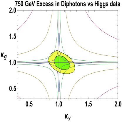
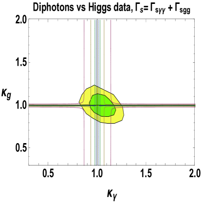
Figure 3: An illustration of the tension between Higgs data and the diphoton excess in minimal scalar models. The curves in the left hand plot are values of $\lambda\Lambda_{c}/N\times 750\,{\rm GeV}=\{0.1,0.05,0.02,0.01\}$ coming in from the outermost curve in Eqn.30. The right hand plot shows $\lambda\Lambda_{c}/N\times 750\,{\rm GeV}=\{0.1,0.05,0.02,0.01\}$ in the case that the width is reproduced by just the gluonic and photon production and decay, given by Eqn.31. In both figures, the curves are overlaid on the $68\%$ and $95\%$ CL curves from the run I Atlas-CMS Higgs combination, fitting only to $\kappa_{g},\kappa_{\gamma}$ ATLAS-CONF-2015-044 .

This conflict can be relaxed in a linear fashion if the excess decreases from its reference value of $8[fb]$ or the width decreases from its reference value of $45\,{\rm GeV}$. However, the inconsistency for order one mixing angles is at the level of four orders of magnitude. The coupling of $S$ to $H^{\dagger}\,H$ that scales as a fourth power must be suppressed from "natural" values to restore consistency with run I data. By the same token, the suppression does not have to be dramatic. An order of magnitude to the fourth power in suppression makes the scenario consistent, considering the experimental uncertainties on the small excess at $750\,{\rm GeV}$. Two orders of magnitude suppression in the coupling of coupling of $S$ to $H^{\dagger}\,H$ restores good agreement with low-energy Higgs data, and such a suppression is not strongly challenged by naturalness concerns.

2.5.2 Reproducing the Width

If we further fix the condition that $\Gamma_{s}=\Gamma(s\rightarrow\gamma\,\gamma)+\Gamma(s\rightarrow gg)$, we derive the constraint equation to reproduce the excess

$$\frac{\Delta\sigma\left(pp\to S\to\gamma\gamma\right)}{8[fb]}\left(\frac{\lambda\Lambda_{c}}{Nm_{s}}\right)^{2}=0.06\,N^{2}\,\left(\kappa_{\gamma}-1\right)^{2}\frac{\left(\kappa_{g}-1\right)^{2}+4.2\times 10^{-6}\left(\kappa_{\gamma}-1\right)^{2}}{\left(\kappa_{g}-1\right)^{2}+0.017\left(\kappa_{\gamma}-1\right)^{2}}$$ (31)

The effects of this condition are shown in Fig.3. Note that reducing the width in this case quickly allows consistency with lower energy data, by making the coupling required to reproduce the excess smaller.

2.5.3 Matching Domination

As we have stressed, the Wilson coefficients $C_{HB}$ and $C_{HG}$ also receive contributions independent of the mixing angle. As these matching coefficients are generated by loops involving two insertions of the new scalar’s coupling to SM field strengths, they lead to a relation between the measured excess and Higgs data which scales as just a square rather than a fourth power.

In the limit where these matching contributions are the only contribution to the shifts in the Higgs couplings and $\lambda_{3}\gg\frac{y_{h}^{2}\,g_{1}^{2}}{2}$, we can express the signal rate as

$$\frac{\Delta\sigma(pp\rightarrow S\rightarrow\gamma\,\gamma)}{8[fb]}\left(\frac{\Gamma_{s}}{45\,{\rm GeV}}\right)=\frac{1.7\times 10^{5}}{\lambda_{3}^{2}}\left(\kappa_{\gamma}-1\right)\left(\left(\kappa_{g}-1\right)+1.5\times 10^{-4}\left(\kappa_{\gamma}-1\right)\right).$$

These matching contributions to the Higgs observables are not significantly constrained by the run I Higgs data.

3 Consistency of pseudoscalar models with lower energy data

A $J^{P}=0^{-}$ pseudoscalar boson interpretation of the $S$ particle related to the diphoton excess would not lead to direct mix with the $J^{P}=0^{+}$ Higgs boson. This further protects this model from related low-energy phenomenology constraints. At the one-loop level such interactions still generate $H^{\dagger}HB^{\mu\,\nu}\,B_{\mu\,\nu}$ through the diagrams shown in Fig.2. We have calculated these contributions and found them to be identical to the scalar case; therefore, the discussion in Section 2.5.3 applies in full to pseudoscalar models. This leaves models which employ a fundamental pseudoscalar to explain the diphoton excess largely unconstrained.

However, the constraints on mixing discussed above still apply to a heavy sector with such a state, which generally arise when the pseudoscalar being considered is a bound state of new strong dynamics. To elaborate on this point concretely, we utilize the models discussed in Ref. Harigaya:2015ezk . Consider a minimal "hidden pion" model of a pseudoscalar given in Ref. Harigaya:2015ezk , which also introduces heavy vector-like hidden quarks at the scale $\Lambda_{c}$, and a new $SU(N)$ gauge group. This leads to the effective interactions of the "hidden pion" $\phi$

$$\mathcal{L}_{\phi}=c_{\tilde{G}}^{\phi}\,\frac{\phi}{f}\,G^{\mu\,\nu}\,\tilde{G}_{\mu\,\nu}+c_{\tilde{B}}^{\phi}\,\frac{\phi}{f}\,B^{\mu\,\nu}\,\tilde{B}_{\mu\,\nu}$$ (33)

with $\tilde{G}_{\mu\,\nu}=\frac{1}{2}\epsilon_{\mu\,\nu\,\sigma\,\rho}G^{\sigma\,\rho}$, and for this model

$$c_{\tilde{G}}^{\phi}=-\frac{N\,g_{3}^{2}}{32\,\sqrt{6}\,\pi^{2}},\quad\,\quad c_{\tilde{B}}^{\phi}=-\frac{9\,(a^{2}-b^{2})\,N\,g_{1}^{2}}{80\,\sqrt{6}\,\pi^{2}},$$ (34)

where $a,b$ are the hypercharges of the constituent particles. In this case the decay to diphotons is considered as analogous to that of the neutral pion, where the decay is calculable and due to the chiral anomaly. Accompanying new scalar mesons of the new confining interactions are generically expected. These scalars will be bounded by the mixing constraints determined in the previous sections. The QCD example is the very wide $\sigma$ meson, which decays dominantly as $\sigma\rightarrow\pi\,\pi$, but does have a known decay into $\gamma\,\gamma$. We can develop a very rough understanding of the relationship between the couplings of a composite pseudoscalar to photons and those of a corresponding scalar on the basis of the constituent dynamics; one expects that the corresponding couplings are related by

$$\frac{c_{\tilde{B}}^{S}}{c_{\tilde{B}}^{\phi}}\sim\frac{a^{2}+b^{2}}{a^{2}-b^{2}}\,\frac{\Psi^{s}(0)}{\Psi^{\phi}(0)}$$ (35)

Figure 4: Anomaly diagrams for $\phi$ and $s$.

here $\Psi^{s}(0)$ and $\Psi^{\phi}(0)$ are the wavefunctions at the origin of the bound states. This is expected if the constituents mediating the coupling to two photons are identical, leading to the same loop function for two mesons. This corresponds to considering a scalar with identical flavor quantum numbers as the pseudoscalar. In the pseudoscalar case there is an insertion of $\gamma^{5}$ in the diagram leading to the difference between squared hypercharges, while in the scalar case a unit matrix sums the squared charges, see Fig.4.

There is no reason to expect $\Psi^{s}(0)\ll\Psi^{\phi}(0)$ in general. The same reasoning applies to decays to $gg$. Mixing bounds then apply to the new scalar. Although $m_{s}$ can exceed $m_{\phi}$, the typical separation expected is $m_{s}/m_{\phi}\lesssim 4\,\pi$.

4 Conclusions

We have examined the consistency of run I Higgs data and a putative diphoton excess at 750 GeV, considering scalar and pseudoscalar states that have an impact on lower energy phenomenology using the SMEFT formalism. We find that large mixings of a 750 GeV state (i.e. Wilson coefficients of the relevant operator $SH^{\dagger}\,H$ proximate to the cutoff scale) are challenged by these concerns, and have examined the corresponding naturalness bounds on the radiatively generated Wilson coefficient, due to the interactions required to produce the excess in diphotons. In general, we find that once a loop suppression of this Wilson coefficient is introduced, scalar models can be viable, and pseudoscalar models are more protected from dangerous low-energy effects. One-loop matchings due to the pseudoscalar interactions do generate the operator $O_{HB}=H^{\dagger}\,H\,B^{\mu\,\nu}\,B_{\mu\,\nu}$. The diphoton excess is not strongly challenged by consistency with lower energy data we have considered, in the simple scenarios we have examined.

Appendix A One-loop Results

Fig.2a gives the one-loop contribution to the Wilson coefficient $C_{HB}$ matching condition

$$\frac{\Delta^{a}\,C_{HB}(m_{s})\,g_{1}^{2}}{\Lambda^{2}}=\frac{\lambda_{3}}{4\,\pi^{2}}\left[\frac{5}{2}-\frac{\pi}{\sqrt{3}}\right]\,\frac{g_{1}^{4}\,c_{B}^{2}}{\Lambda_{\gamma}^{2}},$$ (36)

while Fig.2b gives the contribution

$$\frac{\Delta^{a}\,C_{HB}(m_{s})\,g_{1}^{2}}{\Lambda^{2}}=\frac{1}{4\,\pi^{2}}\left[-\frac{5}{2}+\frac{\pi^{2}}{12}\right]\,\frac{g_{1}^{6}\,y_{h}^{2}\,c_{B}^{2}}{\Lambda_{\gamma}^{2}},$$ (37)

when calculating the unbroken phase of $\rm SU(2)_{L}\times U(1)_{Y}$ to simplify the matching. Note we take the real part of the amplitude in the matching as the Wilson coefficient of the Hermitian operators are real. Fig.2b vanishes for $C_{HG}$ while Fig.1a is the obvious modification of the quoted result for this operator.

B The total photoproduction cross section

Recent estimates of the combined inelastic-inelastic, elastic-inelastic and elastic-elastic photoproduction Fichet:2015vvy ; Fichet:2016pvq ; Csaki:2016raa give a corrected $C_{\gamma\gamma}=78.3$, which is significantly higher than the estimate reported in Csaki:2015vek (and initially used in this paper) for only the elastic production mechanism. Here we give the formulae arising from this total photoproduction. Utilizing this new coefficient, Equation 5 now reads

$$\frac{\Delta\sigma(pp\rightarrow S\rightarrow\gamma\,\gamma)}{8[fb]}\left(\frac{\Gamma_{s}}{45\,{\rm GeV}}\right)\cong 6546\,\left(\frac{m_{s}^{2}\,c_{B}^{2}}{\Lambda_{\gamma}^{2}}\right)\,\left[\left(\frac{m_{s}^{2}\,c_{G}^{2}}{\Lambda_{g}^{2}}\right)+3.5\times 10^{-5}\,\left(\frac{m_{s}^{2}\,c_{B}^{2}}{\Lambda_{\gamma}^{2}}\right)\right],$$ (38)

and Eqn. 30-31 are $\mathcal{O}\simeq 0.0005\,\left(\kappa_{\gamma}-1\right)^{2}\left[\left(\kappa_{g}-1\right)^{2}+6.2\times 10^{-4}\,\left(\kappa_{\gamma}-1\right)^{2}\right]$

$$\frac{\Delta\sigma\left(pp\to S\to\gamma\gamma\right)}{8[fb]}\left(\frac{\lambda\Lambda_{c}}{Nm_{s}}\right)^{2} = 0.06\,N^{2}\,\left(\kappa_{\gamma}-1\right)^{2}\frac{\left(\kappa_{g}-1\right)^{2}+6.2\times 10^{-4}\left(\kappa_{\gamma}-1\right)^{2}}{\left(\kappa_{g}-1\right)^{2}+0.017\left(\kappa_{\gamma}-1\right)^{2}},$$

$$\frac{\Delta\sigma(pp\rightarrow S\rightarrow\gamma\,\gamma)}{8[fb]}\left(\frac{\Gamma_{s}}{45\,{\rm GeV}}\right) = \frac{1.7\times 10^{5}}{\lambda_{3}^{2}}\left(\kappa_{\gamma}-1\right)\left(\left(\kappa_{g}-1\right)+2.2\times 10^{-2}\left(\kappa_{\gamma}-1\right)\right).$$

The resulting modified bounds are illustrated in Fig.6.

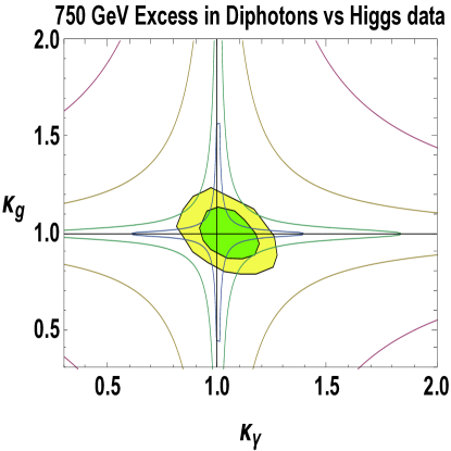
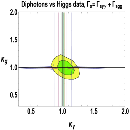
Figure 5: Same as Figure 3, except for the total photoproduction cross section number in the Appendix. The curves in the left hand plot are again values of $\lambda\Lambda_{c}/N\times 750\,{\rm GeV}=\{0.1,0.05,0.02,0.01\}$ coming in from the outermost curve in Eqn.30. The right hand plot shows $\lambda\Lambda_{c}/N\times 750\,{\rm GeV}=\{0.1,0.05,0.02,0.01\}$. In both figures, the curves are overlaid on the $68\%$ and $95\%$ CL curves from the run I Atlas-CMS Higgs combination, fitting only to $\kappa_{g},\kappa_{\gamma}$ ATLAS-CONF-2015-044 .

References

- (1) Search for resonances decaying to photon pairs in 3.2 fb-1 of collisions at = 13 TeV with the ATLAS detector, Tech. Rep. ATLAS-CONF-2015-081, CERN, Geneva, Dec, 2015.
- (2) CMS Collaboration Collaboration, Search for new physics in high mass diphoton events in proton-proton collisions at 13TeV, Tech. Rep. CMS-PAS-EXO-15-004, CERN, Geneva, 2015.
- (3) K. Cranmer, Testing look-elsewhere effect from combining two searches for the same particle using Gaussian Processes, https://github.com/cranmer/look-elsewhere-2d/blob/master/two-experiment-lee.ipynb.
- (4) L. D. Landau, On the angular momentum of a system of two photons, Dokl. Akad. Nauk Ser. Fiz. 60 (1948), no. 2 207–209.
- (5) C.-N. Yang, Selection Rules for the Dematerialization of a Particle Into Two Photons, Phys. Rev. 77 (1950) 242–245.
- (6) C. Csaki, J. Hubisz, and J. Terning, The Minimal Model of a Diphoton Resonance: Production without Gluon Couplings, arXiv:1512.05776.
- (7) S. Fichet, G. von Gersdorff, and C. Royon, Scattering Light by Light at 750 GeV at the LHC, arXiv:1512.05751.
- (8) R. Franceschini, G. F. Giudice, J. F. Kamenik, M. McCullough, A. Pomarol, R. Rattazzi, M. Redi, F. Riva, A. Strumia, and R. Torre, What is the gamma gamma resonance at 750 GeV?, arXiv:1512.04933.
- (9) A. D. Martin, W. J. Stirling, R. S. Thorne, and G. Watt, Parton distributions for the LHC, Eur. Phys. J. C63 (2009) 189–285, [arXiv:0901.0002].
- (10) D. Aloni, K. Blum, A. Dery, A. Efrati, and Y. Nir, On a possible large width 750 GeV diphoton resonance at ATLAS and CMS, arXiv:1512.05778.
- (11) ATLAS Collaboration, G. Aad et al., Search for new resonances in and final states in collisions at TeV with the ATLAS detector, Phys. Lett. B738 (2014) 428–447, [arXiv:1407.8150].
- (12) K. Harigaya and Y. Nomura, Composite Models for the 750 GeV Diphoton Excess, arXiv:1512.04850.
- (13) E. E. Jenkins, A. V. Manohar, and M. Trott, Renormalization Group Evolution of the Standard Model Dimension Six Operators I: Formalism and lambda Dependence, JHEP 1310 (2013) 087, [arXiv:1308.2627].
- (14) E. E. Jenkins, A. V. Manohar, and M. Trott, Renormalization Group Evolution of the Standard Model Dimension Six Operators II: Yukawa Dependence, JHEP 1401 (2014) 035, [arXiv:1310.4838].
- (15) R. Alonso, E. E. Jenkins, A. V. Manohar, and M. Trott, Renormalization Group Evolution of the Standard Model Dimension Six Operators III: Gauge Coupling Dependence and Phenomenology, JHEP 1404 (2014) 159, [arXiv:1312.2014].
- (16) R. Alonso, H.-M. Chang, E. E. Jenkins, A. V. Manohar, and B. Shotwell, Renormalization group evolution of dimension-six baryon number violating operators, Phys.Lett. B734 (2014) 302–307, [arXiv:1405.0486].
- (17) B. Grzadkowski, M. Iskrzynski, M. Misiak, and J. Rosiek, Dimension-Six Terms in the Standard Model Lagrangian, JHEP 1010 (2010) 085, [arXiv:1008.4884].
- (18) R. Contino, M. Ghezzi, C. Grojean, M. Muhlleitner, and M. Spira, Effective Lagrangian for a light Higgs-like scalar, arXiv:1303.3876.
- (19) A. Falkowski, O. Slone, and T. Volansky, Phenomenology of a 750 GeV Singlet, arXiv:1512.05777.
- (20) A. Manohar and H. Georgi, Chiral Quarks and the Nonrelativistic Quark Model, Nucl.Phys. B234 (1984) 189.
- (21) A. V. Manohar, Deep inelastic scattering as x —> 1 using soft collinear effective theory, Phys. Rev. D68 (2003) 114019, [hep-ph/0309176].
- (22) L. Berthier and M. Trott, Consistent constraints on the Standard Model Effective Field Theory, arXiv:1508.05060.
- (23) K. Hagiwara, S. Ishihara, R. Szalapski, and D. Zeppenfeld, Low-energy constraints on electroweak three gauge boson couplings, Phys.Lett. B283 (1992) 353–359.
- (24) S. Alam, S. Dawson, and R. Szalapski, Low-energy constraints on new physics revisited, Phys.Rev. D57 (1998) 1577–1590, [hep-ph/9706542].
- (25) C. Grojean, E. E. Jenkins, A. V. Manohar, and M. Trott, Renormalization Group Scaling of Higgs Operators and Decay , arXiv:1301.2588.
- (26) A. V. Manohar and M. B. Wise, Modifications to the properties of the Higgs boson, Phys.Lett. B636 (2006) 107–113, [hep-ph/0601212].
- (27) Measurements of the Higgs boson production and decay rates and constraints on its couplings from a combined ATLAS and CMS analysis of the LHC pp collision data at = 7 and 8 TeV, Tech. Rep. ATLAS-CONF-2015-044, CERN, Geneva, Sep, 2015.
- (28) A. Alves, A. G. Dias, and K. Sinha, The 750 GeV -cion: Where else should we look for it?, arXiv:1512.06091.
- (29) Y. Bai, J. Berger, and R. Lu, A 750 GeV Dark Pion: Cousin of a Dark G-parity-odd WIMP, arXiv:1512.05779.
- (30) P. Agrawal, J. Fan, B. Heidenreich, M. Reece, and M. Strassler, Experimental Considerations Motivated by the Diphoton Excess at the LHC, arXiv:1512.05775.
- (31) A. Ahmed, B. M. Dillon, B. Grzadkowski, J. F. Gunion, and Y. Jiang, Higgs-radion interpretation of 750 GeV di-photon excess at the LHC, arXiv:1512.05771.
- (32) J. Chakrabortty, A. Choudhury, P. Ghosh, S. Mondal, and T. Srivastava, Di-photon resonance around 750 GeV: shedding light on the theory underneath, arXiv:1512.05767.
- (33) L. Bian, N. Chen, D. Liu, and J. Shu, A hidden confining world on the 750 GeV diphoton excess, arXiv:1512.05759.
- (34) D. Curtin and C. B. Verhaaren, Quirky Explanations for the Diphoton Excess, arXiv:1512.05753.
- (35) W. Chao, R. Huo, and J.-H. Yu, The Minimal Scalar-Stealth Top Interpretation of the Diphoton Excess, arXiv:1512.05738.
- (36) S. V. Demidov and D. S. Gorbunov, On sgoldstino interpretation of the diphoton excess, arXiv:1512.05723.
- (37) J. M. No, V. Sanz, and J. Setford, See-Saw Composite Higgses at the LHC: Linking Naturalness to the GeV Di-Photon Resonance, arXiv:1512.05700.
- (38) D. Becirevic, E. Bertuzzo, O. Sumensari, and R. Z. Funchal, Can the new resonance at LHC be a CP-Odd Higgs boson?, arXiv:1512.05623.
- (39) P. Cox, A. D. Medina, T. S. Ray, and A. Spray, Diphoton Excess at 750 GeV from a Radion in the Bulk-Higgs Scenario, arXiv:1512.05618.
- (40) R. Martinez, F. Ochoa, and C. F. Sierra, Diphoton decay for a GeV scalar boson in an model, arXiv:1512.05617.
- (41) A. Kobakhidze, F. Wang, L. Wu, J. M. Yang, and M. Zhang, LHC 750 GeV diphoton resonance explained as a heavy scalar in top-seesaw model, arXiv:1512.05585.
- (42) S. Matsuzaki and K. Yamawaki, 750 GeV Diphoton Signal from One-Family Walking Technipion, arXiv:1512.05564.
- (43) Q.-H. Cao, Y. Liu, K.-P. Xie, B. Yan, and D.-M. Zhang, A Boost Test of Anomalous Diphoton Resonance at the LHC, arXiv:1512.05542.
- (44) B. Dutta, Y. Gao, T. Ghosh, I. Gogoladze, and T. Li, Interpretation of the diphoton excess at CMS and ATLAS, arXiv:1512.05439.
- (45) C. Petersson and R. Torre, The 750 GeV diphoton excess from the goldstino superpartner, arXiv:1512.05333.
- (46) E. Molinaro, F. Sannino, and N. Vignaroli, Minimal Composite Dynamics versus Axion Origin of the Diphoton excess, arXiv:1512.05334.
- (47) R. S. Gupta, S. J ger, Y. Kats, G. Perez, and E. Stamou, Interpreting a 750 GeV Diphoton Resonance, arXiv:1512.05332.
- (48) B. Bellazzini, R. Franceschini, F. Sala, and J. Serra, Goldstones in Diphotons, arXiv:1512.05330.
- (49) M. Low, A. Tesi, and L.-T. Wang, A pseudoscalar decaying to photon pairs in the early LHC run 2 data, arXiv:1512.05328.
- (50) J. Ellis, S. A. R. Ellis, J. Quevillon, V. Sanz, and T. You, On the Interpretation of a Possible GeV Particle Decaying into , arXiv:1512.05327.
- (51) S. D. McDermott, P. Meade, and H. Ramani, Singlet Scalar Resonances and the Diphoton Excess, arXiv:1512.05326.
- (52) T. Higaki, K. S. Jeong, N. Kitajima, and F. Takahashi, The QCD Axion from Aligned Axions and Diphoton Excess, arXiv:1512.05295.
- (53) S. Di Chiara, L. Marzola, and M. Raidal, First interpretation of the 750 GeV di-photon resonance at the LHC, arXiv:1512.04939.
- (54) A. Pilaftsis, Diphoton Signatures from Heavy Axion Decays at LHC, arXiv:1512.04931.
- (55) D. Buttazzo, A. Greljo, and D. Marzocca, Knocking on New Physics’ door with a Scalar Resonance, arXiv:1512.04929.
- (56) S. Knapen, T. Melia, M. Papucci, and K. Zurek, Rays of light from the LHC, arXiv:1512.04928.
- (57) Y. Nakai, R. Sato, and K. Tobioka, Footprints of New Strong Dynamics via Anomaly, arXiv:1512.04924.
- (58) A. Angelescu, A. Djouadi, and G. Moreau, Scenarii for interpretations of the LHC diphoton excess: two Higgs doublets and vector-like quarks and leptons, arXiv:1512.04921.
- (59) M. Backovic, A. Mariotti, and D. Redigolo, Di-photon excess illuminates Dark Matter, arXiv:1512.04917.
- (60) Y. Mambrini, G. Arcadi, and A. Djouadi, The LHC diphoton resonance and dark matter, arXiv:1512.04913.
- (61) S. Fichet, G. von Gersdorff, and C. Royon, Measuring the diphoton coupling of a 750 GeV resonance, arXiv:1601.01712.
- (62) C. Csaki, J. Hubisz, S. Lombardo, and J. Terning, Gluon vs. Photon Production of a 750 GeV Diphoton Resonance, arXiv:1601.00638.