Testing the validity of the single-spin approximation in inspiral-merger-ringdown waveforms
Abstract
Gravitational-wave signals from black-hole binaries with non-precessing spins are described by four parameters – each black hole’s mass and spin. It has been shown that the dominant spin effects can be modeled by a single spin parameter, leading to the development of several three-parameter waveform models. Previous studies indicate that these models should be adequate for gravitational-wave detection. In this paper we focus on the systematic biases that would result from using them to estimate binary parameters, and consider a one-parameter family of configurations at one choice of mass ratio and effective single spin. We find that for low-mass binaries within that family of configurations, where the observable waveform is dominated by the inspiral, the systematic bias in all physical parameters is smaller than the parameter uncertainty due to degeneracies between the mass ratio and the spins, at least up to signal-to-noise ratios (SNRs) of 50. For higher-mass binaries, where the merger and ringdown make a greater contribution to the observed signal, the bias in the mass ratio is comparable to its uncertainty at SNRs of only 30, and the bias in the measurement of the total spin is larger than the uncertainty defined by the 90% confidence region even at an SNR of only 10. Although this bias may be mitigated in future models by a better choice of single-effective-spin parameter, these results suggest that it may be possible to accurately measure both black-hole spins in intermediate-mass binaries.
pacs:
04.25.Dg, 04.25.Nx, 04.30.Db, 04.30.TvI Introduction
The inspiral and merger of black-hole and neutron-star binaries are the most promising sources for the first direct detection of gravitational waves (GWs) with the Advanced LIGO (aLIGO) and Virgo (AdV) detectors Harry et al. (2010); Acernese et al. (2009); Abadie et al. (2010a), and are expected to provide a wealth of astrophysical information (see, e.g., Sathyaprakash and Schutz (2009)). The optimal technique to locate their signals in the detector data is to cross-correlate the data against a large bank of theoretical signal templates. A search across the full parameter space of component masses, spins, sky locations, orientations and the distance is computationally extremely challenging. Partly for this reason searches in data from the initial LIGO and Virgo detectors Aasi et al. (2013a); Abadie et al. (2012, 2011, 2010b) focussed on binaries with non-spinning components, for which a two-dimensional template bank suffices, greatly reducing the computational cost. The two dimensions are defined by combinations of the component masses, and the effects of the sky-location, orientation and distance on the signal observed by a single detector can be absorbed into an overall amplitude scale factor.
Such simplifications are not possible for generic spinning binaries, where the components’ spins cause precession of the orbital plane and of the spins themselves, leading to far more complex GW signals. However, if we consider only spins aligned/anti-aligned to the binary’s orbital angular momentum, then the only spin effects are on the inspiral rate and the signal amplitude – the basic waveform structure is unchanged from the non-spinning case. Including the aligned/anti-aligned spin effects in the waveform templates makes it possible to detect a much larger volume of the binary parameter space, including in some cases a significant fraction of precessing binaries Ajith et al. (2011); Ajith (2011); Brown et al. (2012). It is also possible that non-precessing-binary models can be used as the basis for constructing generic waveform models Schmidt et al. (2012); Pekowsky et al. (2013). Note that this study analyzes only the modes of the gravitational wave signal.
The inclusion of the (non-precessing) black-hole spins doubles the dimensionality of the search parameter space over non-spinning searches. However, studies of inspiral dynamics using post-Newtonian expansions, and of merger and ringdown with numerical solutions of Einstein’s equations, show that the dominant spin effects can be modeled with a single parameter Ajith et al. (2011); Ajith (2011); Santamaria et al. (2010). This has motivated the development of waveform models parametrized by only the binary’s mass ratio and effective total spin (the binary’s total mass appears as a simple overall scale factor) Vaishnav et al. (2007); Reisswig et al. (2009); Ajith et al. (2011); Ajith (2011); Santamaria et al. (2010). Also, recent work on implementing non-precessing-spin template banks has exploited the partial degeneracy between the two spins Brown et al. (2012); Ajith et al. (2012a).
The use of a single effective spin parameter is also motivated by the high computational cost of fully general relativistic numerical simulations. Work to date on phenomenological waveform models suggests that we require at least four simulations in each direction of parameter space that we wish to model. A model of the full seven-dimensional parameter space of generic binary waveforms would require simulations, which are not feasible before the commissioning of aLIGO and AdV Ajith et al. (2007, 2008); Ajith (2008); Ajith et al. (2011); Santamaria et al. (2010); Hannam and Hawke (2011). The most ambitious study to date includes “only” 200 waveforms, at moderate mass ratios and black-hole spins Mroue et al. (2013). It is therefore important that we exploit any degeneracies that reduce the dimensionality of the parameter space that we must model.
While single-effective-spin models are believed to capture the phenomenology of non-precessing-binary signals with sufficient fidelity for GW detection, little is known about how well they would perform if used to estimate the source parameters following a detection. The single-spin approximation is only valid in the leading-order post-Newtonian spin terms (although it holds to higher order when both masses are equal, and for extreme mass ratios, where the influence of the smaller black hole’s spin is negligible), and does not hold through merger, where the appropriate single spin becomes the total spin angular momentum of the two black holes Buonanno et al. (2008); Rezzolla et al. (2008a); Tichy and Marronetti (2008); Lousto et al. (2010). If we use a single-effective-spin waveform model for parameter estimation, what will be the bias in the measurement of the black-hole masses, and of the spin parameter itself? Obviously, if we approximate the two black-hole spins with a single spin, then we cannot use this model to measure the individual black-hole spins; on the other hand, if a single spin parameter models the dominant spin effects, then both spins will be difficult to measure even if we did use a double-spin model. We will return to this point later.
In this paper we explore the parameter biases due to the use of a single-effective-spin model. Since we expect the single-effective-spin approximation to become less valid for higher mass ratios, we consider a set of configurations at the highest mass ratio of the numerical simulations that were used to calibrate current phenomenological models, 1:4 Ajith et al. (2011); Santamaria et al. (2010). The computational cost of numerical simulations precludes an exhaustive study, so we focus on one value of the effective spin parameter, . (Here and are the masses, and and are the Kerr parameters of the black holes). We produce a set of five simulations with differing values of the individual black-hole spins ( and ), but with the same value of . From the numerical-relativity waveforms we construct hybrid PN-NR waveforms, which are in turn compared against one of the phenomenological models, “IMRPhenomC” (see Sec. II.2 for a more detailed description of the waveform model). By identifying the IMRPhenomC waveform that agrees best with each hybrid, we estimate the parameter biases due to the use of a single-effective-spin model.
There are a number of issues that make it difficult to draw conclusions from this procedure. The results will be skewed by artifacts in the construction of the particular waveform model that we use (the details of the phenomenological ansatz, the coverage of the parameter space by numerical waveforms, and the accuracy of the waveforms), which may swamp the errors due to the single-effective-spin approximation. Previous studies have shown that the main source of uncertainty in hybrid PN-NR waveforms is in the PN regime Hannam et al. (2010); MacDonald et al. (2011); Boyle (2011); Ohme et al. (2011), and as such our results will depend on the PN approximant we use in our hybrids, and on the hybridization frequency. We discuss these issues further, and the steps we have taken to mitigate them, in Sec. V.
The layout of the paper is as follows. We summarize the single-spin approximation, waveforms models and our numerical waveforms in Secs. II and III. In Sec. IV we make a preliminary study of biases in the inspiral regime, where we can compare single- and double-spin PN models using the same PN approximant, and do not have to concern ourselves with issues of hybridization or phenomenological modeling. In addition to quantifying the parameter biases due to the single-effective-spin approximation for low-mass binaries (for mass-ratio 1:4 and moderate spins), this section also provides context and contrast to the full inspiral-merger-ringdown results, which are in Sec. V.
II Preliminaries
II.1 The single-spin approximation
We consider black-hole binaries where the spins are aligned or anti-aligned with the orbital angular momentum. Then the spins and the angular momentum do not precess, which leads to a considerable simplification of the GW signal over generic configurations. These aligned-spin waveforms are parametrized by the black-hole masses and spins.
A single effective spin parameter has been used in the construction of the non-precessing phenomenological inspiral-merger-ringdown (IMR) models presented in Refs. Ajith et al. (2011); Santamaria et al. (2010). These models parametrize the waveforms by their mass , symmetric mass ratio , and the effective spin parameter . They incorporate a PN description of the inspiral, while the merger and ringdown regimes are tuned using the results of numerical simulations. A recent study Ajith (2011) has addressed how well a related “reduced spin” parameter motivated by PN theory works for inspiral searches. This PN model has been shown to be sufficiently accurate for GW searches (“effectual”), and to agree well with the full two-spin waveforms (“faithful”) when either the spins or the masses are equal.
In constructing the PN reduced-spin parameter, we note that all spin effects can be described by two parameters and , which remain constant throughout the evolution. The dimensionless spin parameters are defined as , where is the spin of black hole . The leading order spin term due to spin-orbit coupling appearing at 1.5PN order in the amplitude and the phase can be represented by a single “reduced spin” parameter (see e.g. Ajith (2011); Poisson and Will (1995))
| (1) |
where and .
In contrast, the “effective spin” parameter used in the phenomenological models for black-hole binaries with non-precessing spins Ajith et al. (2011); Santamaria et al. (2010) is defined as a simple mass-weighted linear combination of the spins
| (2) |
For equal masses both spin parameters are a function of the symmetric combination of the spins only. The only difference is an overall factor. For unequal masses both spin parameters depend on the symmetric and anti-symmetric spin combinations. The difference between the spin parameters depends linearly on and therefore goes to zero for infinite mass-ratio.
Historically, the non-precessing phenomenological IMR models to date have used the effective spin parameter defined in Eq. (2) due to its simple form. While this choice was sufficient to build effectual non-precessing waveform models, we will present evidence that suggests that is a better choice and should be used for future models.
II.2 Phenomenological single-spin models
We can quantify the agreement between families of waveforms with the same value of or , but in order to estimate the parameter bias that would result from the single-spin approximation, individual waveforms are not sufficient; we require a waveform family. In this study we compare our PN/NR hybrids with the phenomenological model for black-hole binaries with non-precessing spins presented in Ref. Santamaria et al. (2010). For consistency with the labeling used within the LIGO-Virgo Collaboration LAL we refer to this model as “IMRPhenomC”. (“IMRPhenomA” refers to a model of nonspinning binaries Ajith et al. (2007, 2008); Ajith (2008), and “IMRPhenomB” to an earlier model of non-precessing binaries Ajith et al. (2011); we choose to use “IMRPhenomC” because it incorporates higher-order PN information in the inspiral phasing, but also make cross-checks against the IMRPhenomB model.)
The model waveforms are parametrized by their total mass , symmetric mass ratio , and the effective total spin parameter defined in Eq. (2). The waveform is represented in the Fourier domain as . The amplitude and phase are modeled separately. The IMRPhenomC amplitude is constructed from two parts: a PN inspiral amplitude with the addition of a higher order frequency term, and a ringdown portion, both of which are fit to the model hybrids. For the inspiral portion of the phase IMRPhenomC uses the complete TaylorF2 Sathyaprakash and Dhurandhar (1991); Cutler and Flanagan (1994a); Droz et al. (1999); Ajith et al. (2012b) PN inspiral phasing (up to 3.5PN order, although the spin terms are complete only up to 2.5PN). Only the late inspiral/merger phase is fitted in a narrow frequency range to numerical simulations, while the ringdown waveform is obtained from analytically derived quasi-normal mode expressions for the frequency and attached continuously to the merger phase. For both the amplitude and the phase smooth -window functions are used to connect the individual parts.
The model is a power series in the frequency , and the coefficients in the model are written as polynomials in the two physical parameters and (the total mass is an overall scale factor), and it is the coefficients of these polynomials that are then calibrated to hybrids of PN and NR waveforms. There are 45 free parameters in IMRPhenomC, although the final model is a function of only . The hybrids used to construct IMRPhenomC were produced in the frequency domain, using TaylorF2 for the PN part and a rather broad fitting window . The construction of frequency-domain PN/NR hybrids is discussed in more detail in Sec. III.1.
II.3 Matches, fitting factors and confidence regions
We quantify the agreement between two waveforms, and , with the standard inner product weighted by the power spectral density of a detector Cutler and Flanagan (1994b), called the overlap
| (3) |
The inner product is calculated in terms of the frequency-domain waveforms . The frequency range in which the detector is deemed sensitive is . Let be the normalized frequency-domain waveform. The match between two normalized waveforms is then defined as their inner product, maximized over time and phase shifts of the waveform,
| (4) |
Given a signal waveform with physical parameters and a template with physical parameters we define the fitting factor
| (5) |
Instead of the fitting factor we will often quote the fully optimized mismatch
| (6) |
The match quantifies the physical agreement between two waveforms (since the time of arrival and overall phase of the waveform do not change the underlying physics of the binary). The fitting factor is a measure of how well a matched-filter search with a given waveform family can perform in detecting a particular signal; a fitting factor greater than 0.965 indicates that no more than 10% of signals will be lost in a search. It does not tell us, however, how well the parameters of the best-match template will agree with the true source parameters of the signal.
A PN-NR hybrid binary waveform that has been produced for a given total mass can be trivially rescaled to a different mass. Therefore, the match between two such waveforms can be optimized over the total mass. The phenomenological model “IMRPhenomC” used in this study depends in addition on the symmetric mass-ratio and the effective spin , which allows us to compute fitting factors by optimizing matches over .
In this paper we compare PN-NR hybrids signals with “IMRPhenomC” with reference to the expected sensitivity of the Advanced LIGO detector Abbott et al. (2009); Shoemaker (2009); Harry and the LIGO Scientific Collaboration (2010). Early science runs are expected around 2015 Aasi et al. (2013b). At its optimum sensitivity several years later, the anticipated sensitivity is given by the “zero-detuned high-power” noise curve The LIGO Scientific Collaboration (2009). We use a linear interpolation of this expected PSD and choose Hz, and kHz.
For PN matches we choose the upper frequency of the overlap integral as the frequency of the innermost stable circular orbit (ISCO) of a test particle around a Schwarzschild black hole , where just as in Ajith (2011). The Schwarzschild ISCO is an arbitrary point at which to terminate the PN waveform, but it corresponds to the choice commonly made in detector searches Babak et al. (2013).
The model parameters for the waveform that best matches the signal correspond to the parameters that are most likely to be recovered in a GW measurement. We are also interested in the range of parameters that would be recovered in 90% of observations at a given SNR, i.e., the 90% confidence region for that SNR, which illustrates the statistical uncertainty in the measurement.
At high SNRs the confidence region can be estimated by Fisher-matrix methods Finn and Chernoff (1993); Cutler and Flanagan (1994a); Poisson and Will (1995); Arun et al. (2005), while in general one should construct the full posterior probability distribution function van der Sluys et al. (2008a, b); Veitch and Vecchio (2010); Feroz et al. (2009); Aasi et al. (2013c). The latter is computationally very expensive, but Ref Baird et al. (2013) shows that it is possible to produce a good approximation to the correct confidence region by computing matches between the model waveform with the physical parameters of the signal, and model waveforms with a range of neighboring parameters. All neighbouring waveforms that have a match greater than some threshold are within the 90% confidence region. The threshold for a given SNR assuming a 3-dimensional parameter space is Baird et al. (2013)
| (7) |
where are arbitrary waveform parameters (in this case , , and or ), and are the correct parameters, and are the model waveforms.
We have computed fitting factors and the associated best parameters with two different methods. The Nelder-Mead Amoeba Nelder and Mead (1965) simplex method has been used to compute fitting factors for a range of masses (see Sec. V.2). For selected masses we have computed confidence regions by sampling the matches on a suitably fine grid in space. The latter computation is a lot more expensive, but more reliable — in some cases the amoeba calculation can be trapped in a local minimum, especially when the confidence region in question is not simply connected. At low masses and high SNRs confidence regions can be very elongated filaments and a transformation to rotate and squash the region into a more compact form is then helpful to keep the computation within a reasonable cost. This is related to the alternative parameter-space coordinates that are being used in placing waveforms in search template banks Ohme et al. (2013); Tanaka and Tagoshi (2000); Brown et al. (2012); Pai and Arun (2013).
III Numerical waveforms
To fully test the single-spin approximation across the binary parameter space, we would need to perform, for each of a wide range of choices of and (or , a series of simulations for choices of different black-hole spins that correspond to the same value of (). In doing so, we would have produced enough simulations to construct a complete two-spin waveform model — but the high computational cost of doing so is one of the motivations for producing a single-effective-spin model in the first place!
We expect the single-effective-spin approximation to become less accurate as the binary mass ratio increases, and so in this study we focus on the largest mass ratio that was considered in the numerical simulations used to calibrate current phenomenological models Ajith et al. (2011); Santamaria et al. (2010), . We choose an effective total spin of ; this is a relatively large total effective spin for which we can also choose a wide range of individual black-hole spins.
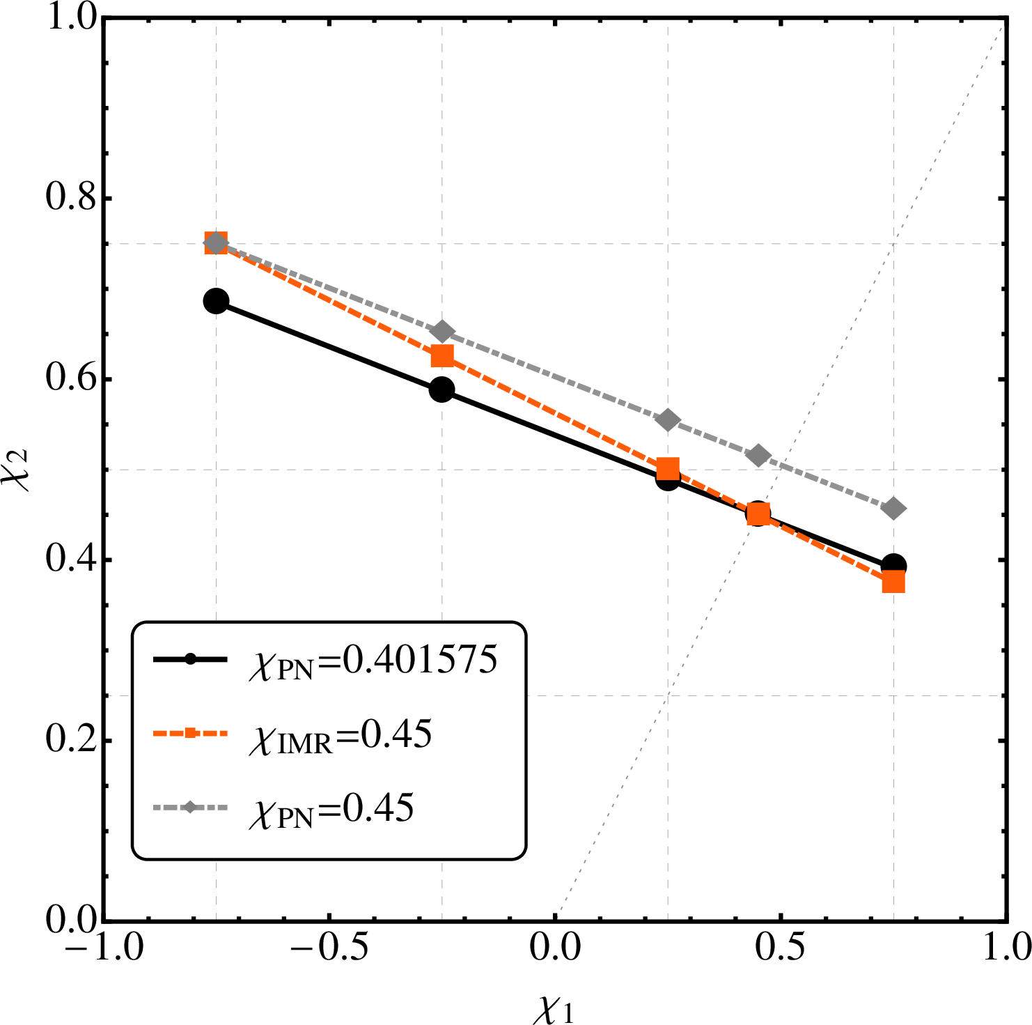
In our simulations we set the total mass and using the convention have and . We then have . With our choice of we let (the spin of the smaller BH), vary between -0.75 and +0.75. (Due to the large junk-radiation content in Bowen-York initial data for highly spinning binaries, we do not consider spins higher than 0.75.) Along this line of in the plane we pick configurations for . In addition we also add the configuration with equal spins . The latter configuration is important since IMRPhenomC Santamaria et al. (2010) assumes equal spins for its PN part. Our chosen configurations are summarized in table 1 (also see Fig. 1).
| Run | Cycles | |||||||
|---|---|---|---|---|---|---|---|---|
| 1 | -0.75 | 0.75 | 44.4 | 29 | 10.739 | 0.0003 | 0.966 | 0.84 |
| 2 | -0.25 | 0.625 | 38.5 | 28 | 10.782 | 0.0006 | 0.969 | 0.79 |
| 3 | 0.25 | 0.5 | 38.5 | 28 | 10.831 | 0.0007 | 0.971 | 0.74 |
| 4 | 0.45 | 0.45 | 38.5 | 28 | 10.853 | 0.0027 | 0.973 | 0.72 |
| 5 | 0.75 | 0.375 | 44.4 | 28 | 10.889 | 0.0014 | 0.972 | 0.68 |
The numerical simulations were performed with the BAM code Brügmann et al. (2008); Husa et al. (2008), which evolves black-hole-binary puncture initial data Brandt and Brügmann (1997); Bowen and York (1980) (generated using a pseudo-spectral elliptic solver Ansorg et al. (2004)), and evolves them with the -variant of the moving-puncture Campanelli et al. (2006); Baker et al. (2006); Hannam et al. (2007) version of the BSSN Shibata and Nakamura (1995); Baumgarte and Shapiro (1999) formulation of the 3+1 Einstein evolution equations. Spatial finite-difference derivatives are sixth-order accurate in the bulk Husa et al. (2008), Kreiss-Oliger dissipation terms converge at fifth order, and a fourth-order Runge-Kutta algorithm is used for the time evolution. The gravitational waves emitted by the binary are calculated from the Newman-Penrose scalar , and the details of our implementation of this procedure are given in Brügmann et al. (2008).
The basic grid setup for this study is based on a setup used for a convergence series of , simulations. In general, the mass-ratio has the most significant impact on choosing a grid setup, since the apparent horizons (AH) of the black holes must be resolved by the finest grid level. We have found that choosing the size of the innermost box about a factor the size of the AH of the smaller BH leads to good accuracy. Since the spin of the smaller BH varies in the five configurations considered in this study, the individual grid setup is tuned differently for each simulation. We found that sufficient accuracy could be achieved by using a minimum of 16 buffer zones (rather than the formal requirement of 32) between mesh-refinement boxes. The Courant factor has been reduced to (from in our previous work) to curb the contribution of time-integration error to the overall NR error. A detailed study of the accuracy of these simulations, and the effects of the errors due to both the spatial finite-differencing and the timestepping, will be presented in a forthcoming paper Husa et al. (2013).
We have performed two iterations of the eccentricity reduction method detailed in Ref. Pürrer et al. (2012) for each of the configurations. The final eccentricities are below 0.0015. The numerical waveforms are obtained by extracting the mode of at .
While we have not performed convergence tests for the NR waveforms, we expect that the results are robust because we have used a “safe” grid setup that has led to accurate results for related aligned-spin configurations with q=4 and . In Sec. V.2 we show how the numerical resolution affects fitting factors and biases of the waveform with IMRPhenomC, and find that it does not affect our overall results.
III.1 Construction and accuracy of PN-NR hybrid waveforms
The NR waveforms we have computed for this study do not cover the full aLIGO sensitivity band for lower-mass binaries. Therefore we need to hybridize the NR waveform with a PN approximant. Different choices are possible for constructing such PN-NR hybrids (see Ref. Ajith et al. (2012b) for a summary). We wish to compare our IMR hybrids with the IMRPhenomC model, in which the inspiral is modeled by the TaylorF2 frequency-domain PN approximant. In order to minimize effects arising from differing PN approximants, we choose to create hybrids with TaylorF2.
We use a frequency domain hybridization method as described in Santamaria et al. (2010). We include the NR waveform data from the time immediately after the passage of the burst of initial junk radiation, up to the point where the ringdown is dominated by numerical noise, and apply a Planck tapering window McKechan et al. (2010) of width M at the start of the dataset. The waveform is further padded with zeroes before computing the FFT to increase the frequency resolution. The NR strain is calculated in the Fourier domain as . The matching procedure aligns and by a least squares fit over a fitting interval , which we discuss in more detail below. We then determine the matching frequency at which the NR and PN phases coincide by a root-finding algorithm. The PN and NR amplitudes are aligned separately without any freedom to adjust parameters.
After having settled on an approximant and choice of hybridization method we can still choose the frequency region over which the hybridization is performed. Intuitively it makes sense to hybridize at as low a frequency as possible so as to extract as much useful information from the NR data as we can, and to minimize errors in the PN approximant, which increase with GW frequency. It also stands to reason that the matching interval should not be too narrow as the fit would then be prone to pick up spurious oscillations in the NR data. For the hybrids considered in this study we have chosen an interval length of and a matching frequency of about . This results in a relative matching width of and is consistent with the choice advocated in Ref. MacDonald et al. (2011).
One accessible measure to gauge the quality of a hybrid are the parameter errors given by the least squares fit. At first glance a high quality fit appears to be very desirable. However, the PN model used in the fit gives a worse approximation of the NR phase as we go to higher frequencies and thus small standard errors in the fitting parameters do not necessarily imply that the hybrid will be very faithful.
In a practical sense it is useful to think of the difference between hybrids with varying hybridization regions (assuming reasonable comparison interval, i.e. not unreasonably high frequencies) as a way of quantifying the error in the hybrid caused by the PN and NR data. We would like to know how such variations in the hybrid construction manifest themselves in biases and uncertainties. In Sec. V.2 we verify that our results are robust with respect to hybridization artifacts.
IV Results for PN single-effective-spin models
A single-effective-spin PN model has recently Ajith (2011) been shown to be an effective search template (i.e., fitting factors ) as well as “faithful” to two-spin signals (i.e., non-optimized matches are also ), when either the spins or the masses are equal. Here we address the question of biases and uncertainties incurred by the single-effective-spin approximation. While there is a preferred “reduced-spin” parameter in the PN regime, we also generalize the model used in Ref. Ajith (2011) to arbitrary definitions of an effective spin parameter and compare with a model built from , the effective spin parameter used by current phenomenological waveform models.
The construction of a single-effective-spin model is straightforward. We choose one based on the TaylorF2 approximant. The model is based on the mapping , where is an arbitrary effective spin parameter. To build the model an inverse of this mapping is needed which requires a relation between and . We choose to use only the symmetric part of the input spins (i.e., setting ) and define the frequency domain single spin model strain as
| (8) |
With this definition the model represents equal spin configurations exactly. For the choice this model is identical to the one defined in Ref. Ajith (2011).
We choose the following mass-ratio configurations for the comparison of single spin PN models (see Fig. 1). For the model we select the same cases along (orange, dashed) as used for NR simulations. The configurations for the model are chosen along a line (black solid), rather than (gray, dot-dashed). The reason is that intersects at the equal spin configuration, for which both models are exact. For and the symmetric combination of the spins vanishes and thus at this point. The largest deviation between the spin parameters happens at the largest positive spin of the smaller BH and is about .
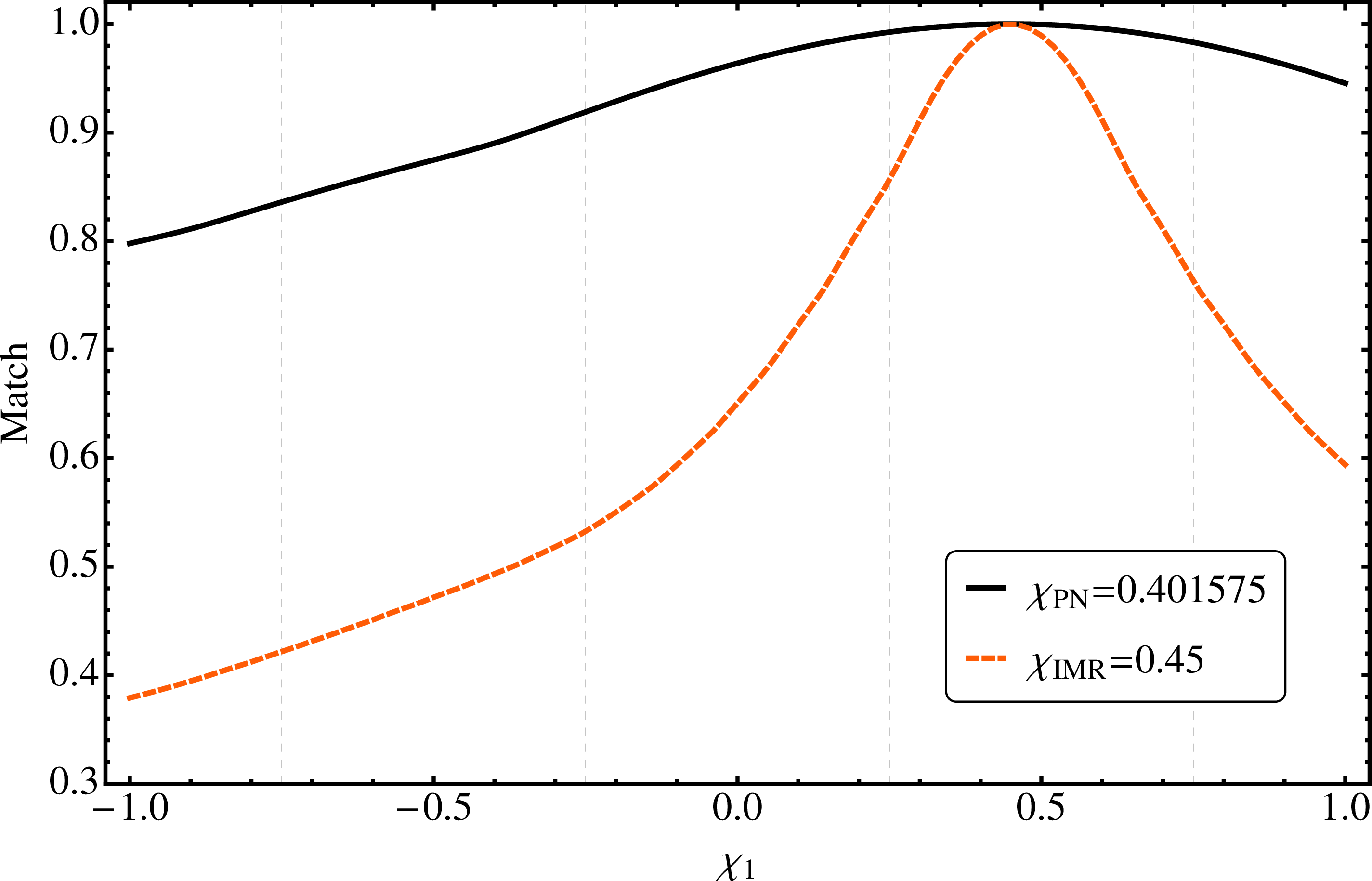
It is well known that is the (almost) optimal single-effective-spin parameter in the PN regime (this combination appears explicitly in the leading-order spin-orbit coupling) Ajith (2011); Poisson and Will (1995). The superiority of over is illustrated in Fig. 2 by how quickly matches between a single spin model (based on either or ) and TaylorF2 signals (again at constant or , respectively) degrade when one moves away from the point , where the models are exact, along a line of the respective .
As an example we compute fully optimized matches (fitting factors) and parameter biases for TayorF2 signal waveforms chosen as above with each of the single spin models for a system mass of . To quantify the statistical uncertainty we also calculate confidence regions in the 3-dimensional space of model parameters .
From an astrophysical point of view, a compact binary with could correspond to an actual NS-BH binary with component masses . The NS would be expected to have very small spin which is contrary to some of the configurations chosen here. However, our goal is to compare how well the single spin approximation works in the PN and IMR regimes (see Sec. V.2) and therefore we choose the same range of spin values for both PN and IMR models.
The results are summarized in Tabs. 2 and 3. The fully optimized mismatches (see Eq. (6)) have been computed from confidence regions at SNR 50 which will be discussed later. We have performed a least-squares fit to the elongated direction of the filament-like confidence regions and subsequently carried out a local minimization starting from the best match found along the curve fit. Although the knowledge of the confidence regions is not needed to compute fitting factors this method leads to more reliable results than simpler optimization methods.
We define biases as , where is one of the model parameters . Note that in tabs. 2 and 3 we have dropped the subscript PN/IMR in the relative bias of the spin parameters. For ease of comparison we also give the absolute bias in the spin.
| Case | Mismatch | ||||
|---|---|---|---|---|---|
| (-0.75, 0.685104) | |||||
| (-0.25, 0.587144) | |||||
| (0.25, 0.489184) | |||||
| (0.45, 0.45) | |||||
| (0.75, 0.391224) |
| Case | Mismatch | ||||
|---|---|---|---|---|---|
| (-0.75, 0.75) | |||||
| (-0.25, 0.625) | |||||
| (0.25, 0.5) | |||||
| (0.45, 0.45) | 0 | ||||
| (0.75, 0.375) |
The fitting factors for both single-effective-spin models are very high, with the fully optimized mismatch below . The models are exact at the equal-spin configuration and therefore the true parameters are recovered. As we move away from the equal-spin configuration the mismatch becomes larger and the parameter biases increase. The bias in the chirp mass is overall very small, below , consistent with standard results. This is expected since the leading factor in the PN phase evolution for non-precessing binaries is proportional to , which is dominated by the chirp mass Finn and Chernoff (1993); Arun et al. (2005); Baird et al. (2013). In contrast, there is considerable bias in the spin parameter and symmetric mass-ratio for the very unequal spin configurations. For the -model the modulus of the biases in and increases to about for the configuration with , which is the farthest from the equal-spin case. The biases are worse for the -model and reach about for the configuration. The absolute spin bias is at most for , while it rises to twice that value for .
We know from PN theory that provides a better single-effective-spin approximation at low masses, but these results quantify the difference in parameter biases in using either or . The bias resulting from the use of is up to twice as large as that due to using a model parametrized by .
At first glance, the results in Tabs. 2 and 3 suggest that the single-effective-spin approximation is entirely inappropriate for parameter estimation: the uncertainty in the mass ratio and the spin parameter can be as high as %, even if we use the approximation. This in turn suggests that, if a single-effective-spin approximation behaves poorly, then we may be able to accurately resolve the individual black-hole spins with a complete two-spin model. Before making this conclusion, we should consider the statistical uncertainty in the parameter measurement for likely aLIGO and AdV SNRs.
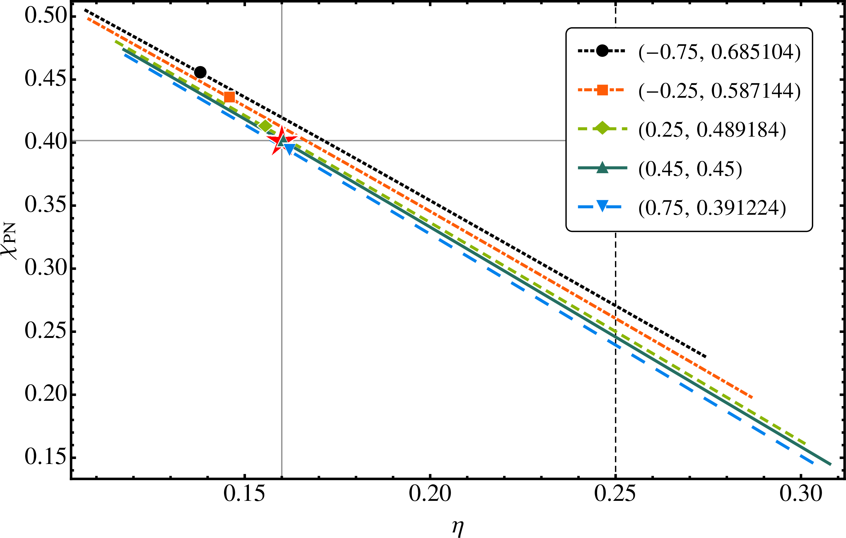
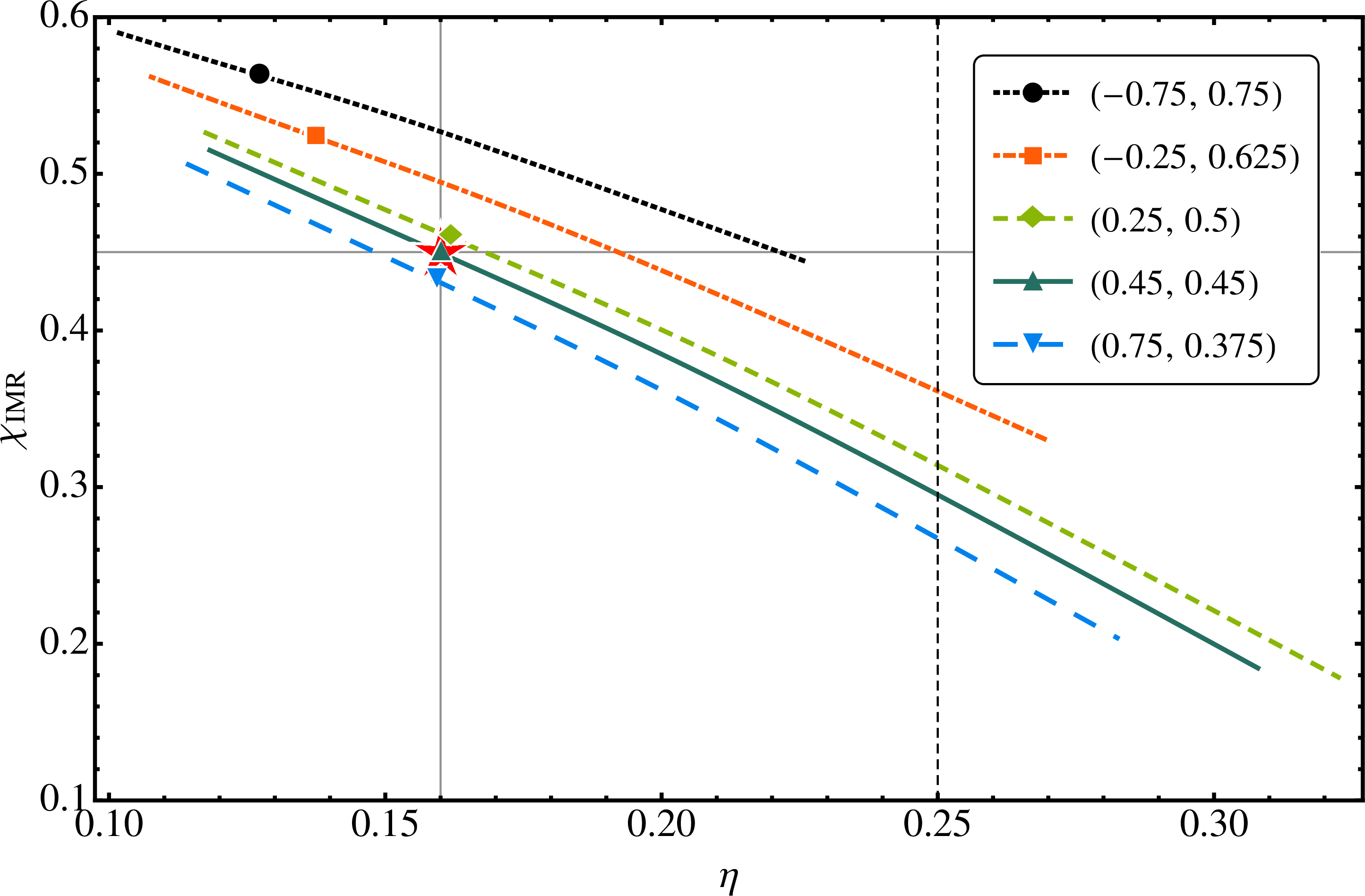
The non-detection of signals in first-generation detectors suggests that events with SNRs higher than 30 will be rare in second-generation detectors Lindblom et al. (2008). This should be borne in mind when we consider Fig. 3, which shows the 90% confidence regions (see Eq. (7)) for a much higher SNR of 50. The confidence regions correspond to a binary, and show results for both single-effective-spin PN models. We project the 3-dimensional confidence regions in onto the symmetric mass-ratio and effective spin . The optimal parameters are denoted by colored symbols, while the true parameters are shown by red stars. At this mass and high SNR the confidence regions are very elongated filaments and we choose to depict them by a curve fit through center of the regions. The regions shown for the equal-spin configuration (solid dark green) are the confidence regions in the proper sense as the signal is exactly represented by the models at this point. For the waveforms that do not lie in the model subspaces the confidence regions are computed with the model waveform that has the best match with the given signal. The very large uncertainty given by the extent of the confidence regions in Fig. 3 is due to the (approximate) degeneracy between mass-ratio and spin Cutler and Flanagan (1994a); Poisson and Will (1995); Baird et al. (2013); Hannam et al. (2013). One can see from the leading order spin-orbit term that it is possible to mimic the effect of spin by modifying the mass-ratio at constant chirp mass.
The uncertainties for the model are about and . For the model the uncertainties are comparable, but a bit larger, roughly and . For both models the confidence regions extend into the region of unphysical . If we project the confidence regions onto the plane of component masses all configurations lie on top of a line of constant chirp mass . For both models the configurations range from an equal-mass binary with total mass up to a mass-ratio binary with total mass , as opposed to the true parameters . These results are consistent with those shown in Ref. Hannam et al. (2013), and illustrate the point made in that work, that we would not be able to determine if such a source was a binary containing two black holes, or a black hole and a neutron star.
We can quantify the additional uncertainty introduced by the single spin approximation with a given parameter or by comparing the “spread” in between the recovered parameters with the extent of the model confidence region in the direction. For the -model we find a spread vs a spread of for the model. The extent of the equal-spin confidence regions in is roughly for and for . For both models at the chosen mass of the statistical uncertainties dwarf the spread in the biases, even at this high SNR of 50. In addition, note that all of the recovered parameters for the model are within the statistical error bars of the “true” parameters.
These results demonstrate that, while the systematic parameter biases from the single-effective-spin models may appear large, they are in fact much smaller than the statistical errors, even at high SNR. We conclude, then, that the reduced-spin model presented in Ref. Ajith (2011) is likely to be sufficient for parameter estimation of low-mass signals from aLIGO and AdV.
V Results for IMR waveforms
V.1 Matches between IMR waveforms
We now consider the family of PN-NR hybrid waveforms summarized in Tab. 1.
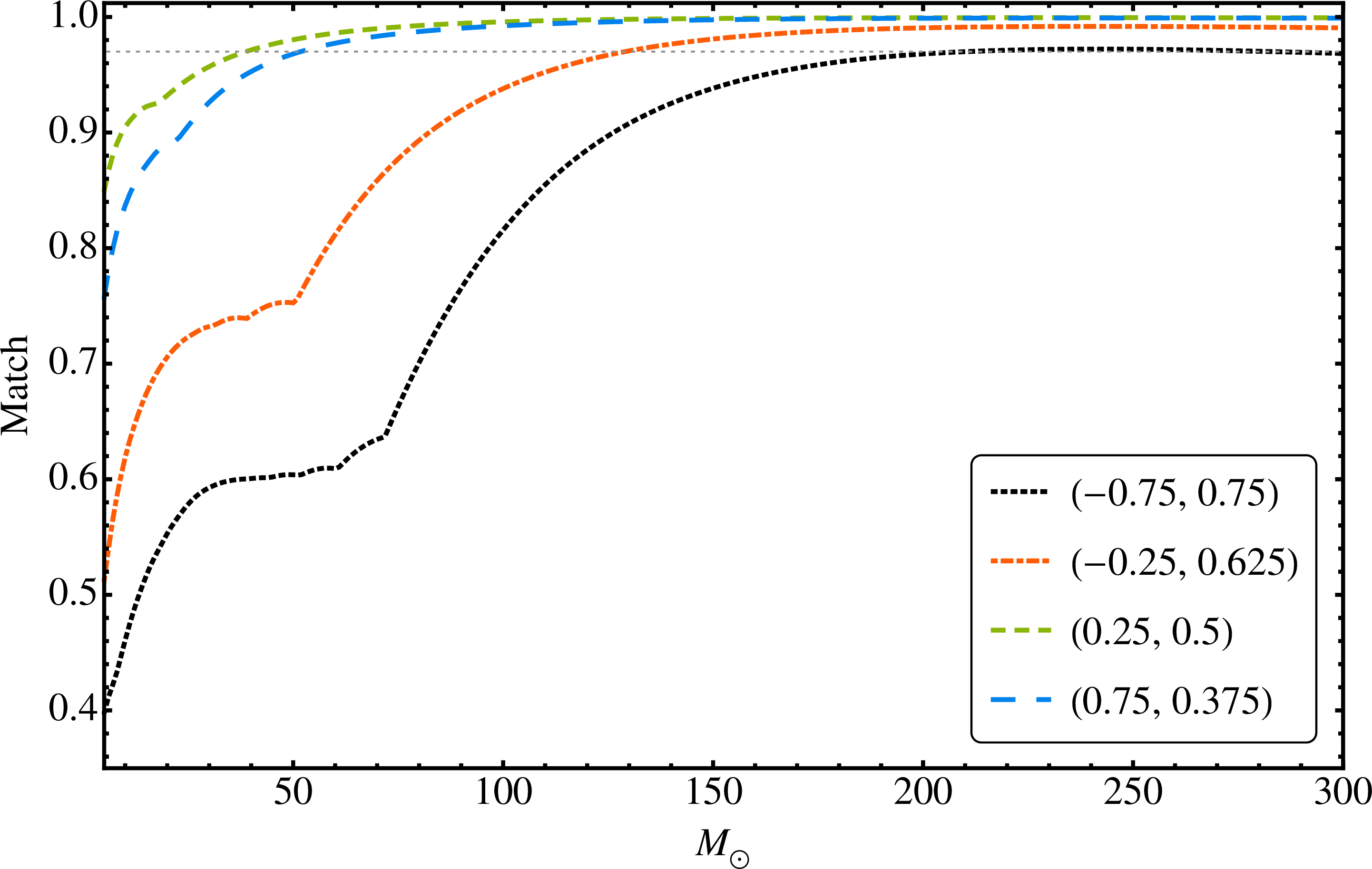
In Fig. 4 we show matches between the TaylorF2 frequency-domain hybrid (see Sec. III.1) of the reference case, with each of the other configurations listed in Tab. 1. As we would expect, the further away the individual spins are from the fiducial waveform the worse the matches become.
The degradation of the matches for low masses is expected due to the use of the parameter; the configurations used in this study lie along a line of . The configuration corresponds to . Fig. 1 shows how these lines diverge. Those configurations for which the spread between these lines is the largest (i.e., those that are the farthest away from the fiducial configuration) are therefore expected to have the worst match. In fact, for low masses, the matches between these IMR waveforms are very close to the PN matches computed at in Fig. 2, as expected.
Around hybridization artifacts lead to a visible kink in the matches. Note that these are not artifacts of the hybridization procedure itself, but rather a result of the disagreement between the TaylorF2 and fully general relativistic NR waveforms at the matching frequency; these artifacts could be made arbitrarily small if we produced NR waveforms of sufficient length to match to PN at arbitrarily low frequencies. Previous studies of NR waveform length requirement (in particular Ref. Ohme et al. (2011)), and the estimates of statistical uncertainties in this study, suggest that the measurement errors due to these effects do not have a significant impact on the scientific information that can be extracted from aLIGO and AdV GW observations.
As we go to higher masses the matches improve considerably, which indicates that in the merger regime performs well. Beyond the matches drop off as we move away from the fiducial configuration due to the different final spin and thus different ringdown frequency of the remnant BHs.
It is very likely that the matches between waveforms along a line of constant would be far higher even through the merger and ringdown. Again, our results are consistent with our expectation from PN theory that future phenomenological models should be parametrized by .
V.2 Biases and uncertainties against IMRPhenomC
As with the TaylorF2 reduced-spin PN model in Sec. IV, we now wish to study the parameter biases due to the use of the single-effective-spin in full inspiral-merger-ringdown waveform models. For this purpose we will compare our family of constant PN-NR hybrids against one of the current phenomenological IMR models, IMRPhenomC. Our goal is complicated by a number of factors. One class of error sources in our analysis is the accuracy of the hybrid waveforms: this will depend on the accuracy of the NR waveforms, on the frequency at which they are hybridized to PN waveforms, and the accuracy of the PN approximant that was used. These errors are mitigated by choosing the same PN approximant, TaylorF2, as was used for the inspiral part of IMRPhenomC. The two other sources of uncertainty (hybridization frequency and NR-waveform accuracy), can be quantified, and we will show (in Figs. 12 and 13) that they do not affect our conclusions.
A more serious source of error is in the IMRPhenomC model itself. This model was calibrated to NR waveforms up to mass ratio 1:4, but not spinning-binary waveforms at that mass ratio. The hybrids that we compare with the model are therefore at the very edge of the region of parameter space over which the model was calibrated. In addition, IMRPhenomC (and all current phenomenological models in general) were designed with detection in mind, and not as a tool for parameter estimation. There are certainly errors in how well IMRPhenomC represents the hybrid waveforms from which it was built, i.e. modeling errors, as well as hybridization artifacts due to the waveform length, and errors in the NR simulations that were used. From these combined error sources we expect a bias in the parameters that we estimate using this model, which will be nontrivially combined with the errors due to the use of the single-effective-spin approximation, which are the biases we wish to measure in this study. The other error sources can be reduced in future phenomenological models, while the bias due to the single-effective-spin approximation will be inherent in all such models.
Despite these complications, we are able to draw a number of important conclusions from our results, which we discuss in this section.
The first point to emphasize is that, despite all of the shortcomings outlined above, the IMRPhenomC model achieves its main purpose as a search template family. We show fully optimized mismatches with IMRPhenomC in Fig. 5. All of them are below . This confirms the effectualness of IMRPhenomC in this region of the parameter space, and the suitability of the model for aligned-spin GW searches. Let us contrast these results of IMRPhenomC with its predecessor IMRPheomB: Due to its simpler PN part IMRPhenomB is only effectual for masses for the configurations considered here.
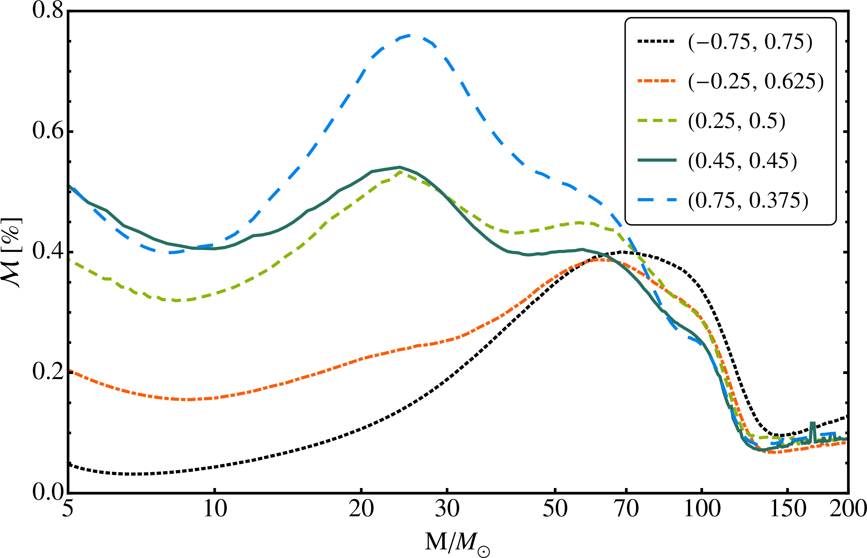
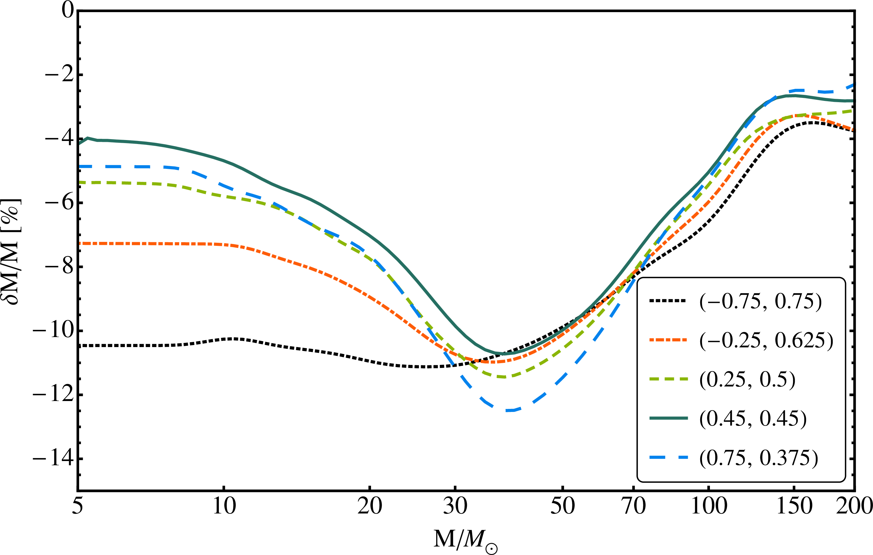
Biases of the total binary mass, as a function of the total mass of the signal, are shown in Fig. 6. This figure illustrates well the complications that were discussed above in our comparisons with IMRPhenomC. The reference waveform has spins , and should be identical to the waveform in the model. The bias in the total mass for this case is therefore most likely due to modeling artifacts in IMRPhenomC. If we are to assess the bias due only to the use of the single-effective-spin approximation, then we must look at the spread of the parameters away from the (solid) line in the figure. We then see that the spread in the total mass can be as high as 5% at low masses (due in most part, once again, to the parametrization by instead of ) and no more than 2% at intermediate masses. At high masses the spread in the total mass is around 1%.
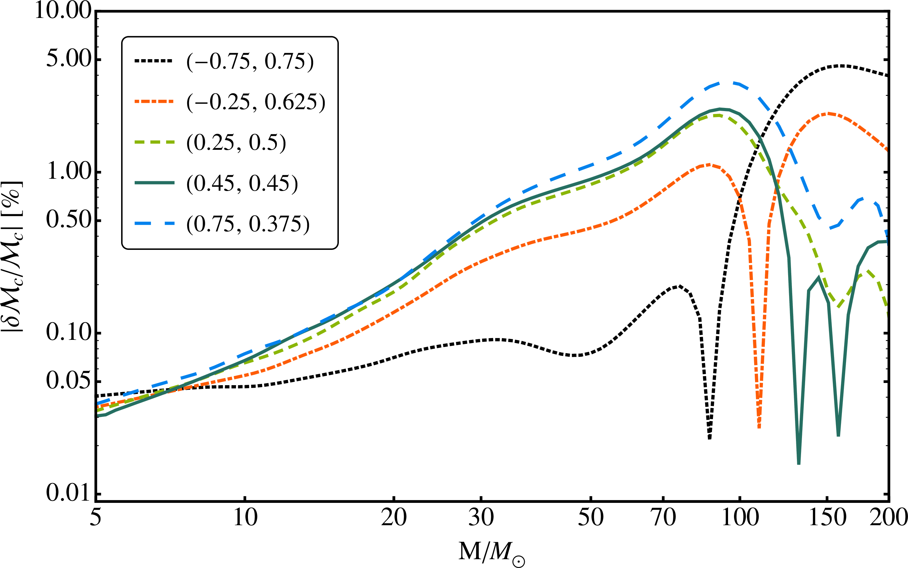
The bias in the chirp mass is shown in Fig. 7. For inspiral signals, we expect to be able to measure the chirp mass extremely accurately, because it is the leading-order PN contribution; that is the motivation for the definition of the chirp mass. And indeed the bias in the chip mass is below 0.1% for masses below 10 . However, the chirp mass has little significance during merger and ringdown, and the chirp-mass bias increases for higher-mass binaries; the fractional error in the chirp mass is comparable to (and in some cases larger than) that in the total mass above 50 . Note that the dips in the curves in the figure are due to the use of a logarithmic scale; these are points where changes sign.
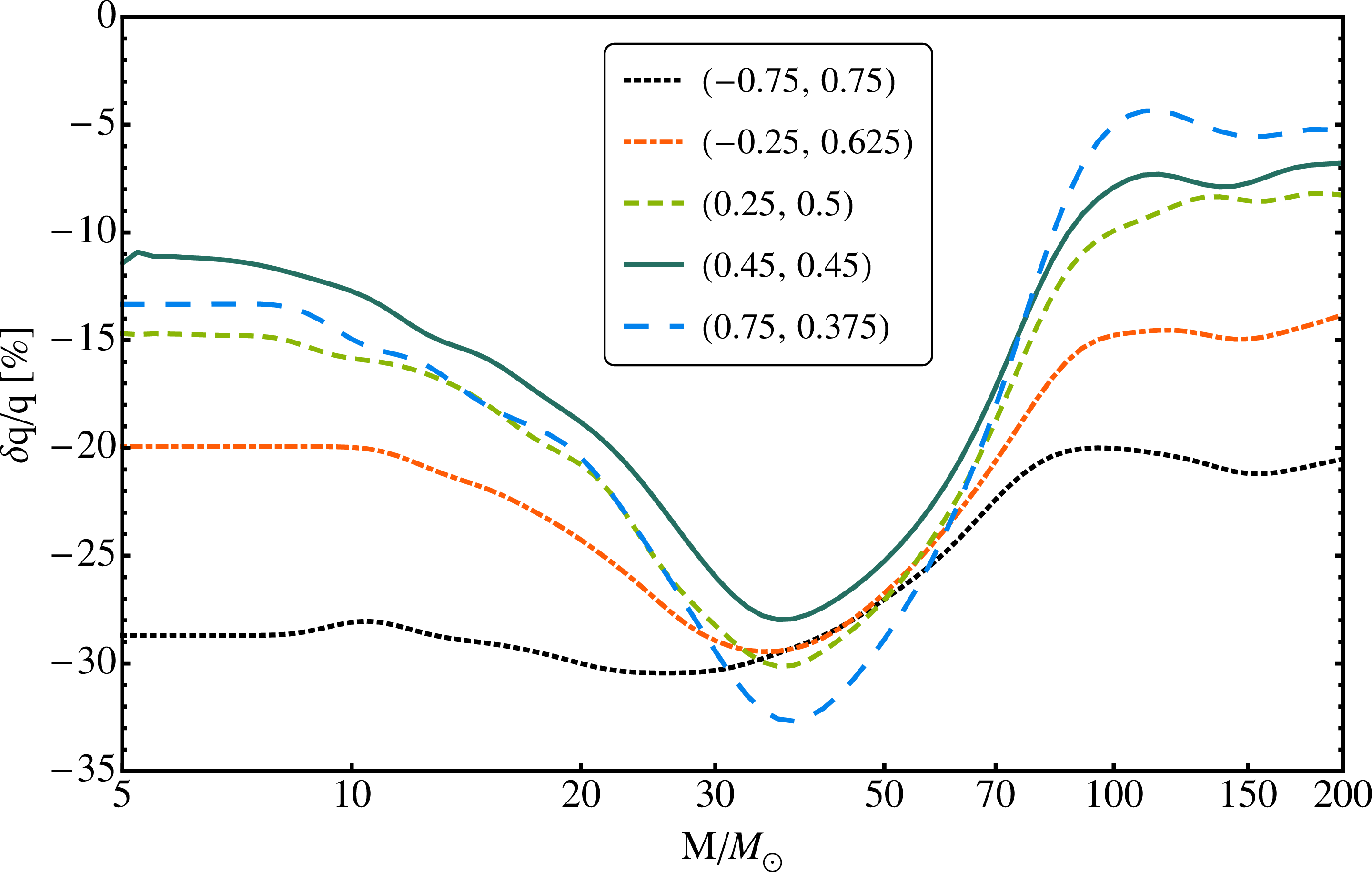
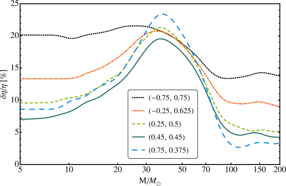
The biases in mass ratio and the symmetric mass-ratio are shown in Fig. 8. Once again, to interpret these figures in terms of the bias due to the single-effective-spin approximation, we should consider the spread of values around the lines. We see for the mass ratio, the spread in values is around 20% for high-mass systems. (At low masses, the results are again exaggerated by the use of the parameter.)
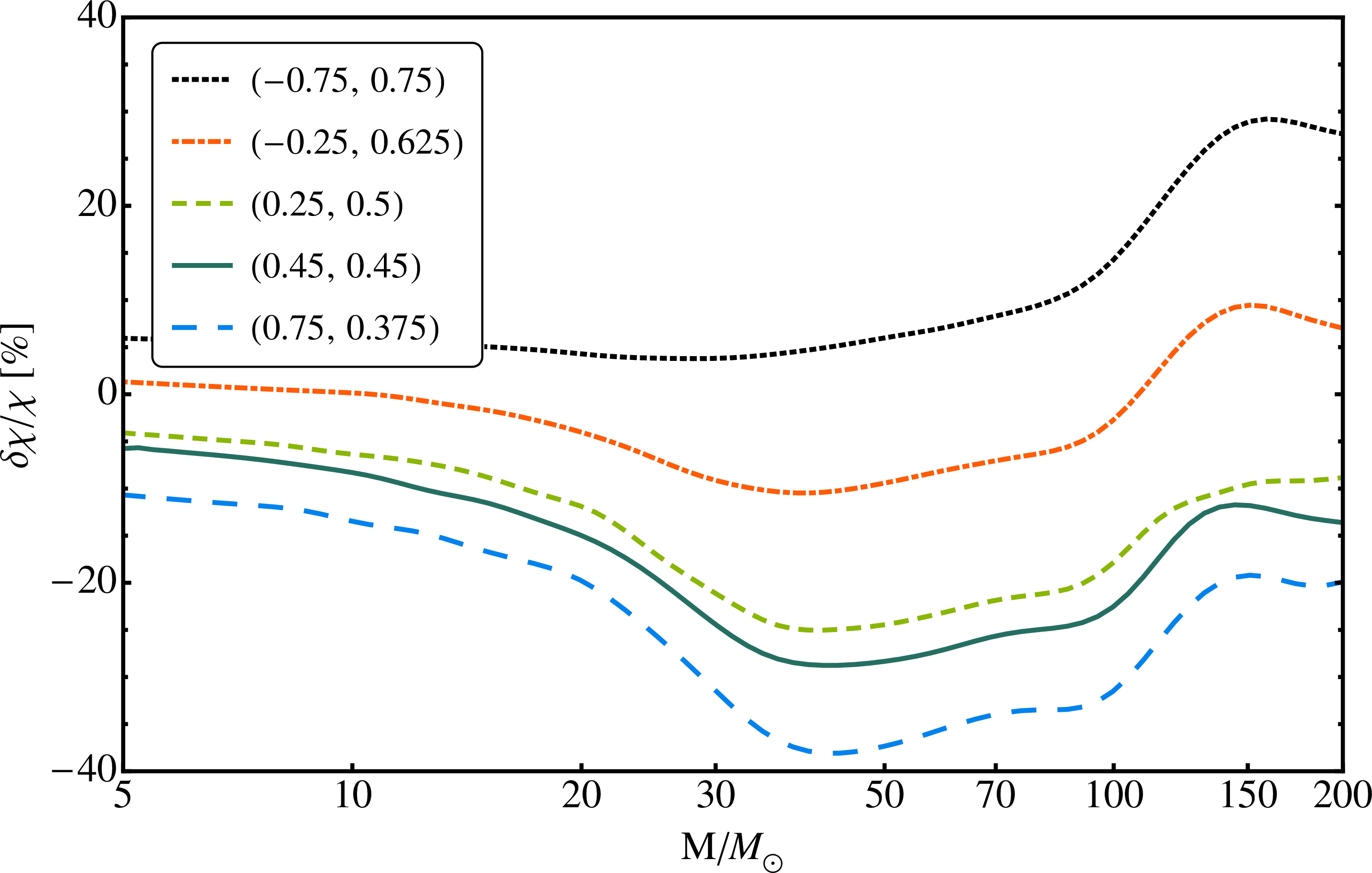
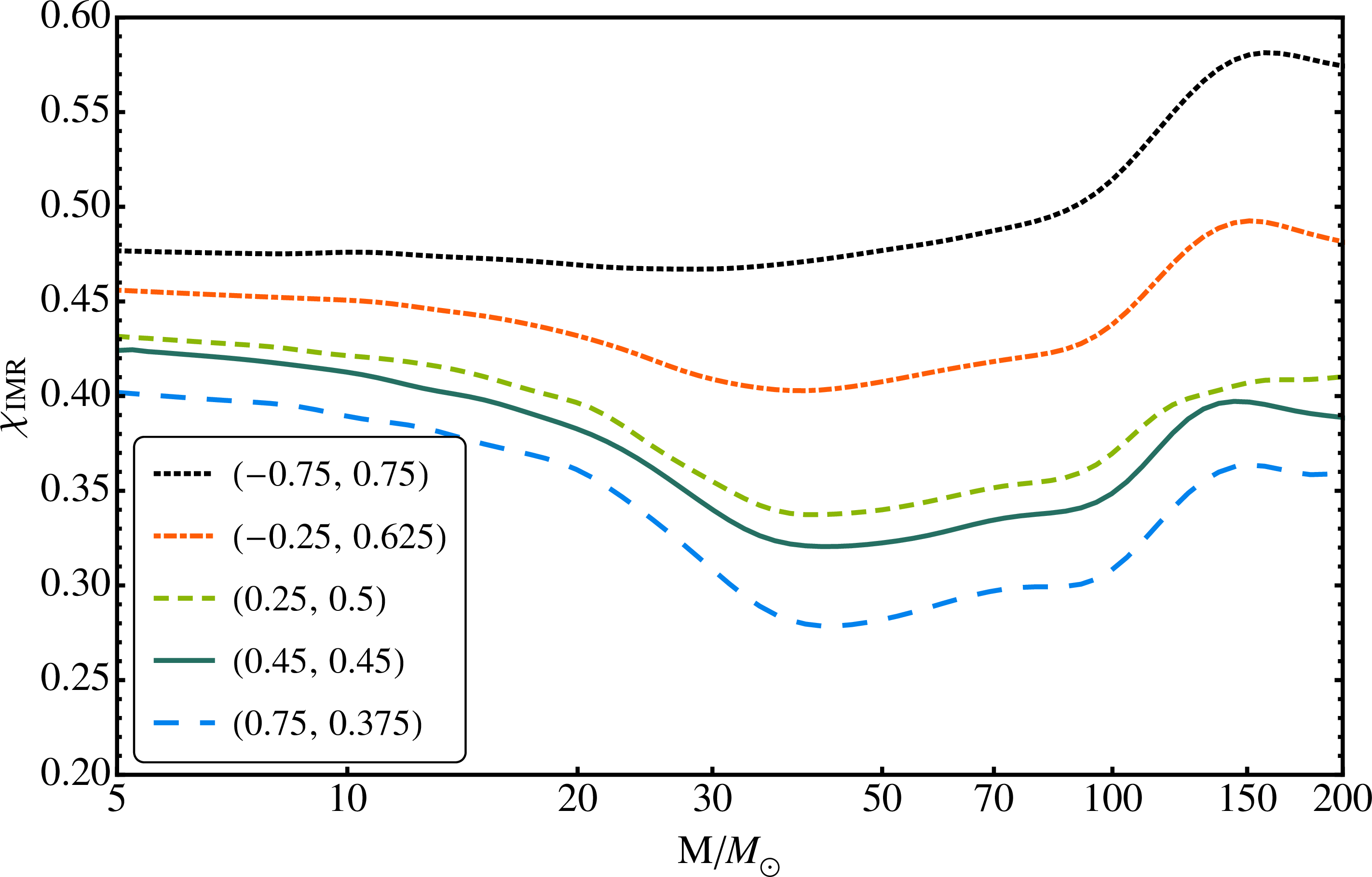
The biases in the spin parameter and the recovered spin values themselves are shown in Fig. 9. At low masses it makes sense to compare the results with the findings of Sec. IV where we studied single spin PN models. The PN model using is the relevant one to compare with. The biases are in general consistent between our PN and IMR studies: very low in , of similar magnitude in and . The spread in the biases is a little smaller, about for the IMR results, as opposed to for PN. The difference in the PN and IMR confidence regions, even at low masses, was also noted in Ref. Hannam et al. (2013), and will be studied further in future work.
| Case | Mismatch | recovered | |||
|---|---|---|---|---|---|
| (-0.75,0.75) | |||||
| (-0.25,0.625) | |||||
| (0.25,0.5) | |||||
| (0.45,0.45) | |||||
| (0.75,0.375) |
As in the PN study in Sec. IV, the spread in biases needs to be put into context with the statistical uncertainty in the parameter measurements. For comparison, Fig. 10 shows the confidence regions (see Eq. (7)) for a 50 binary and table 4 summarizes the biases at this mass. While the extent of the confidence regions is much more confined than was the case for the PN models, the regions are still elongated in a diagonal direction in and and illustrate the degeneracy between mass-ratio and spin Baird et al. (2013). We see that the uncertainty in the masses is in general larger than the spread in the parameter biases. For example, the spread in values at 50 was 5%, while the statistical uncertainty in the mass ratio at SNR 30 is 10% (see Fig. 10). We can conclude, then, that the single-effective-spin approximation does not adversely affect estimation of the black-hole masses at likely advanced-detector SNRs.
| Mass | |||
| Spread in biases | 0.11 | 0.22 | 0.2 |
| Extent of CR in SNR 10 | 0.16 | 0.22 | 0.41 |
| Extent of CR in SNR 20 | 0.07 | 0.1 | 0.2 |
| Comparable SNR | 13 | 10 | 20 |
The situation is quite different for the spin parameter. At 50 , the recovered spin parameter has a spread of , while the statistical uncertainty in becomes comparable at SNR 10. For higher SNRs the spread in the spin bias dominates.
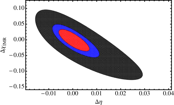
We focus on the bias in in Tab. 5. We concentrate on the spread of the biases and therefore ignore the offset in the average bias of the IMR configurations from the true value, due to the model not being faithful in this region of the parameter space. The spread of recovered parameter values gives us an indication of the additional uncertainties introduced by the single-effective-spin approximation. We find that the single spin approximation is valid for to SNR 10 for masses and up to SNR 20 for . Results for IMRPhenomB lead to comparable conclusions.
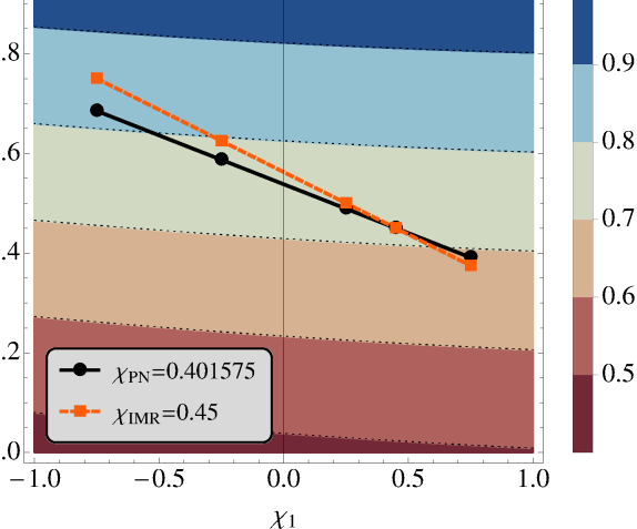
We have noted in Sec. V.1 that the waveform from the ringdown of the final black hole will be characterized by the final spin, and not by either or . We illustrate this point in Fig. 11, where we overlay the curves of constant and on the contours of constant final spin, which can be predicted by a number of formulas in the literature Tichy and Marronetti (2008); Barausse and Rezzolla (2009); Rezzolla et al. (2008b); Buonanno et al. (2008); Lousto et al. (2010). The results of the various final-spin formulas agree to within a few percent with our numerical results for the final spins (see Tab. 1) with the largest disagreement at the (-0.75,0.75) configuration. We see that configurations with the same value of either spin parameter during inspiral can lead to a black hole with a wide range of final spins, depending on the individual spins of the progenitor black holes. (In Tab. 1 we see that final spins for our family of numerical simulations ranges from 0.68 up to 0.84.)
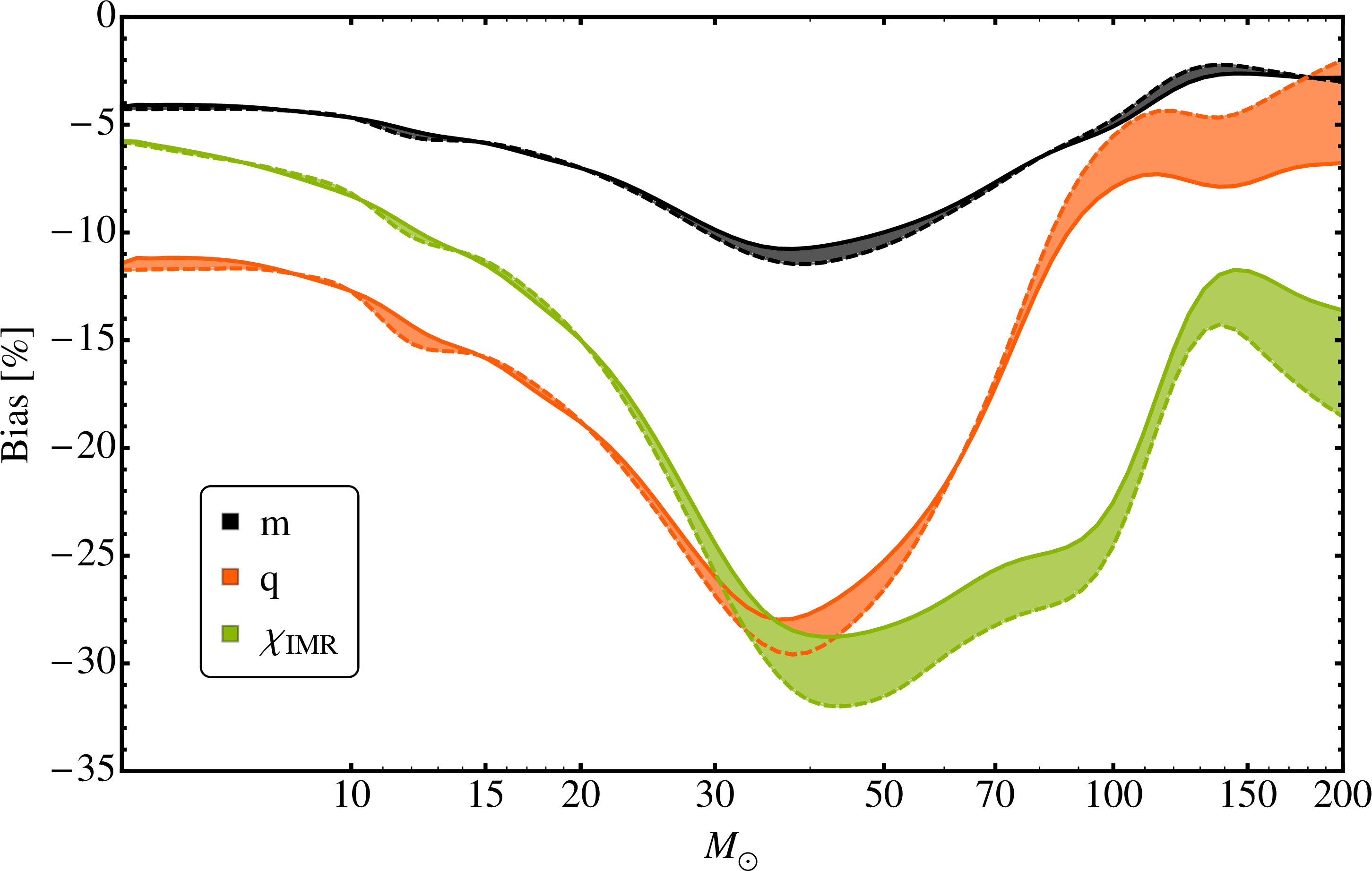
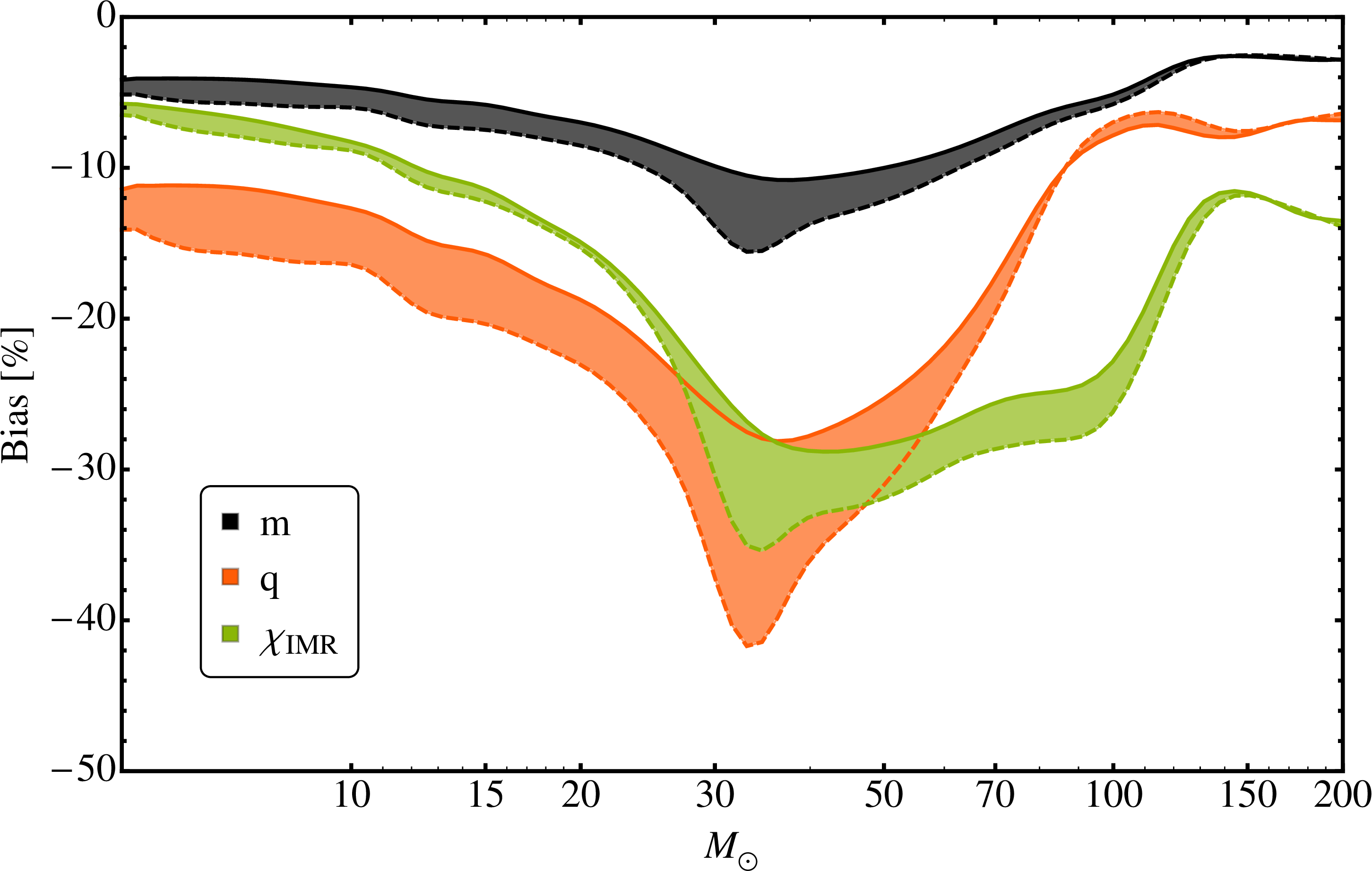
Finally, we verify that our results are not qualitatively changed by errors in the numerical-relativity waveforms or artifacts due to the choice of hybridization frequency. Fig. 12 compares the variation in biases caused by changing the resolution of the numerical waveform used to construct the hybrid, while Fig. 13 shows the effect of changing the hybridization frequency. Changing the NR resolution only manifests itself at higher masses (both hybrids have been constructed at comparable matching frequencies ), whereas changing the hybrid parameter affects predominantly low to medium masses. While this is not an in-depth error analysis, it gives an indication of how sensitive our results are to these two sources of errors that we can control. It is clear from the figures that neither of these error sources appears to be a serious issue in most cases, but does warrant further study in the future.
VI Conclusions
Several non-precessing-binary waveform models make use of the observation that the effects of the black-hole spins on the inspiral rate can be approximated by a single effective spin parameter, either in the case of a reduced-spin inspiral model Ajith (2011), or for phenomenological inspiral-merger-ringdown models Ajith et al. (2011); Santamaria et al. (2010). (The two parameters are defined in Eqns. (1) and (2).) These models were developed primarily for use in template banks for gravitational-wave searches, but they have also been used for parameter estimation Aasi et al. (2013c). We have investigated the systematic bias in parameter measurement due to the use of these single-effective-spin approximations.
Our primary goal has been to explore the parameter bias from phenomenological waveform models, and for this purpose we focussed on a family of numerical-relativity simulations of binaries with mass ratio 1:4, and all with (but with different values of individual spins). Fig. 4 shows that the noise-weighted inner product (match) between these waveforms is in general larger than 0.97 for masses greater than 200 , but the match degrades significantly at lower masses. We note that if we had parameterized these waveforms instead by a constant value of , then their matches would be much better at low masses, since we know that the waveforms are partially degenerate in in the low-frequency (post-Newtonian) regime.
In assessing systematic parameter biases, we first consider the inspiral regime, and study two related families of post-Newtonian waveforms, one with and the other (again, with varying individual spins). Here we find that, for signal-to-noise ratios below 50 (and we expect most observations in aLIGO and AdV to be below 30), the statistical uncertainty in the measurement of both the masses and the spin () is significantly larger than the parameter bias incurred by using the single-effective-spin-approximation model to estimate the parameters. This result is discussed in detail in Sec. IV, and summarized here in the upper panel of Fig. 14. Although limited to only one point in the parameter space, this result suggests that the reduced-spin inspiral model is sufficiently accurate for parameter estimation from GW observations in aLIGO and AdV.
We then consider the hybrid PN-NR inspiral-merger-ringdown waveforms (with constant ), and compare them against the IMRPhenomC model. Our first observation is that, while the IMRPhenomC model performs well for detection purposes, with all fitting factors 0.99 (see Fig. 5), artifacts in the construction of the waveform model cause a significant systematic bias even for the equal-spin waveform that should be reproduced by the model with . This problem can be removed in future by producing a model calibrated against NR waveforms across a larger volume of parameter space, and such work is already underway. The bias we observe at low masses (see Figs. 6, 8, and 9) is consistent with our choice of as our single-effective-spin parameter, and suggests that future phenomenological models should be parameterized instead with .
Our main observation from these results is that at intermediate masses (around 50 ) the spread in recovered spin values is far larger than the statistical uncertainty in , even at an SNR of 10, which is close to the detection threshold. This can be seen in Figs. 9 and 10, and is summarized here in the lower panel of Fig. 14, which shows the deviation in the parameter measurement from the value obtained for the reference waveform.
The small parameter bias due to the single-effective-spin approximation at low masses implies that the approximation holds well at these masses, and therefore that it will be difficult to measure the component spins in low-mass binaries. This is the unfortunate corollary of the validity of the single-effective-spin approximation: GW searches can be more efficient, but parameter estimation is less accurate.
Since we observe large parameter biases at intermediate masses, this implies that in these cases we may be able to measure the individual spins. It is quite likely that there is a strong degeneracy between the two spins and the mass ratio at all stages in the binary’s evolution, but if we observe a waveform in which the early part (the inspiral) is characterized by , and the late part (the ringdown) is characterized by the final spin, then it is likely that to describe the full waveform we require knowledge of both black-hole spins. If this is the case, then it follows that accurate measurements of both spins may be possible. This is an interesting topic for further work.
This study analyzes only the modes of the gravitational wave signal. The amplitude of higher order modes is sensitive to the mass-ratio, and thus could serve to break degeneracies between and in parameter estimation. However, it should be borne in mind that at the mass-ratios that this model is calibrated at the higher modes are all much weaker than the 22-mode and at the low SNRs considered here we do not expect our results to change appreciably.
Do these results imply that we should construct a two-spin non-precessing model? Not necessarily. A single-effective-spin model is sufficient for detection, and, following detection, if the source is a black-hole-binary with total mass 50 , then we could perform addition simulations with varying individual black-hole spins, and produce a localized model for parameter estimation purposes. We note that although it is possible to produce sufficient waveforms to cover the non-precessing-binary parameter space in time for the commissioning of aLIGO and AdV, a higher priority may be to produce models that approximately cover the full precessing-binary parameter space, for which it would be more efficient to model the spins parallel to the orbital angular momentum by only a single parameter.
Further work is needed to verify the spread of the parameter biases in the spin in the IMR waveforms, using updated phenomenological waveform models, and studies across a larger volume of the parameter space. In assessing our ability to measure either an effective single spin parameter, or both black-hole spins, we also need to quantify the influence of harmonics beyond the dominant modes.
VII Acknowledgements
We thank S. Fairhurst, F. Ohme, H. Pfeiffer, S. Khan, B. Sathyaprakash, and P. Schmidt for useful discussions and comments. M. Hannam was supported Science and Technology Facilities Council grants ST/H008438/1 and ST/I001085/1. S. Husa was supported by grant FPA-2007-60220 from the Spanish Ministry of Science and the Spanish MICINN’s Consolider-Ingenio 2010 Programme under grant MultiDark CSD2009-00064. M. Pürrer thanks Caltech and the Universitat de les Illes Balears (UIB) for hospitality. BAM simulations were carried out at Advanced Research Computing (ARCCA) at Cardiff, and as part of the European PRACE petascale computing initiative on the clusters Hermit, Curie and SuperMUC.
References
- Harry et al. (2010) G. M. Harry et al. (LIGO Scientific Collaboration), Class.Quant.Grav. 27, 084006 (2010).
- Acernese et al. (2009) F. Acernese et al. (The Virgo Collaboration), Advanced Virgo Baseline Design (2009), [Virgo Techincal Document VIR-0027A-09].
- Abadie et al. (2010a) J. Abadie et al. (LIGO Scientific), Class. Quant. Grav. 27, 173001 (2010a), eprint 1003.2480.
- Sathyaprakash and Schutz (2009) B. Sathyaprakash and B. Schutz, Living Rev.Rel. 12, 2 (2009), eprint http://www.livingreviews.org/lrr-2009-2.
- Aasi et al. (2013a) J. Aasi et al. (LIGO Scientific Collaboration, Virgo Collaboration), Phys. Rev. D 87, 022002, 022002 (2013a), eprint 1209.6533.
- Abadie et al. (2012) J. Abadie et al. (LIGO Collaboration, Virgo Collaboration), Phys.Rev. D85, 082002 (2012), eprint 1111.7314.
- Abadie et al. (2011) J. Abadie et al. (LIGO Scientific Collaboration, Virgo Collaboration), Phys.Rev. D83, 122005 (2011), eprint 1102.3781.
- Abadie et al. (2010b) J. Abadie et al. (LIGO Scientific Collaboration, Virgo Collaboration), Phys.Rev. D82, 102001 (2010b), eprint 1005.4655.
- Ajith et al. (2011) P. Ajith, M. Hannam, S. Husa, Y. Chen, B. Bruegmann, et al., Phys.Rev.Lett. 106, 241101 (2011), eprint 0909.2867.
- Ajith (2011) P. Ajith, Phys.Rev. D84, 084037 (2011), eprint 1107.1267.
- Brown et al. (2012) D. A. Brown, I. Harry, A. Lundgren, and A. H. Nitz, Phys.Rev. D86, 084017 (2012), eprint 1207.6406.
- Schmidt et al. (2012) P. Schmidt, M. Hannam, and S. Husa, Phys.Rev. D86, 104063 (2012), eprint 1207.3088.
- Pekowsky et al. (2013) L. Pekowsky, R. O’Shaughnessy, J. Healy, and D. Shoemaker (2013), eprint 1304.3176.
- Santamaria et al. (2010) L. Santamaria et al., Phys. Rev. D82, 064016 (2010), eprint 1005.3306.
- Vaishnav et al. (2007) B. Vaishnav, I. Hinder, F. Herrmann, and D. Shoemaker, Phys. Rev. D76, 084020 (2007), eprint 0705.3829.
- Reisswig et al. (2009) C. Reisswig et al., Phys. Rev. D80, 124026 (2009), eprint 0907.0462.
- Ajith et al. (2012a) P. Ajith, N. Fotopoulos, S. Privitera, A. Neunzert, and A. Weinstein (2012a), eprint 1210.6666.
- Ajith et al. (2007) P. Ajith et al., Class. Quant. Grav. 24, S689 (2007), eprint 0704.3764.
- Ajith et al. (2008) P. Ajith et al., Phys. Rev. D77, 104017 (2008), eprint 0710.2335.
- Ajith (2008) P. Ajith, Class. Quant. Grav. 25, 114033 (2008), eprint 0712.0343.
- Hannam and Hawke (2011) M. Hannam and I. Hawke, Gen.Rel.Grav. 43, 465 (2011), eprint 0908.3139.
- Mroue et al. (2013) A. H. Mroue, M. A. Scheel, B. Szilagyi, H. P. Pfeiffer, M. Boyle, et al. (2013), eprint 1304.6077.
- Buonanno et al. (2008) A. Buonanno, L. E. Kidder, and L. Lehner, Phys. Rev. D77, 026004 (2008).
- Rezzolla et al. (2008a) L. Rezzolla et al., Astrophys. J. 674, L29 (2008a), eprint 0710.3345.
- Tichy and Marronetti (2008) W. Tichy and P. Marronetti, Phys.Rev. D78, 081501 (2008), eprint 0807.2985.
- Lousto et al. (2010) C. O. Lousto, M. Campanelli, and Y. Zlochower, Class. Quant. Grav. 27, 114006 (2010), eprint 0904.3541.
- Hannam et al. (2010) M. Hannam, S. Husa, F. Ohme, and P. Ajith, Phys.Rev. D82, 124052 (2010), eprint 1008.2961.
- MacDonald et al. (2011) I. MacDonald, S. Nissanke, H. P. Pfeiffer, and H. P. Pfeiffer, Class.Quant.Grav. 28, 134002 (2011), eprint 1102.5128.
- Boyle (2011) M. Boyle, Phys.Rev. D84, 064013 (2011), eprint 1103.5088.
- Ohme et al. (2011) F. Ohme, M. Hannam, and S. Husa, Phys.Rev. D84, 064029 (2011), eprint 1107.0996.
- Poisson and Will (1995) E. Poisson and C. M. Will, Phys.Rev. D52, 848 (1995), eprint gr-qc/9502040.
- (32) LSC algorithm library (LAL), URL http://www.lsc-group.phys.uwm.edu/lal.
- Sathyaprakash and Dhurandhar (1991) B. Sathyaprakash and S. Dhurandhar, Phys.Rev. D44, 3819 (1991).
- Cutler and Flanagan (1994a) C. Cutler and E. E. Flanagan, Phys.Rev. D49, 2658 (1994a).
- Droz et al. (1999) S. Droz, D. J. Knapp, E. Poisson, and B. J. Owen, Phys. Rev. D 59, 124016 (1999), eprint gr-qc/9901076.
- Ajith et al. (2012b) P. Ajith, M. Boyle, D. A. Brown, B. Brugmann, L. T. Buchman, et al., Class.Quant.Grav. 29, 124001 (2012b), eprint 1201.5319.
- Cutler and Flanagan (1994b) C. Cutler and E. E. Flanagan, Phys. Rev. D 49, 2658 (1994b).
- Abbott et al. (2009) B. Abbott et al. (LIGO Scientific), Rept. Prog. Phys. 72, 076901 (2009), eprint 0711.3041.
- Shoemaker (2009) D. Shoemaker (the Advanced LIGO Team), Advanced LIGO Reference Design (2009), [LIGO-M060056].
- Harry and the LIGO Scientific Collaboration (2010) G. M. Harry and the LIGO Scientific Collaboration, Class. Quant. Grav. 27, 084006 (2010).
- Aasi et al. (2013b) J. Aasi et al. (LIGO Scientific Collaboration, Virgo Collaboration) (2013b), eprint 1304.0670.
- The LIGO Scientific Collaboration (2009) The LIGO Scientific Collaboration, Tech. Rep. LIGO-T0900288-v3, LIGO Project (2009), URL https://dcc.ligo.org/DocDB/0002/T0900288/003/AdvLIGO%20noise%20curves.pdf.
- Babak et al. (2013) S. Babak, R. Biswas, P. Brady, D. Brown, K. Cannon, et al., Phys.Rev. D87, 024033 (2013), eprint 1208.3491.
- Finn and Chernoff (1993) L. S. Finn and D. F. Chernoff, Phys.Rev. D47, 2198 (1993), eprint gr-qc/9301003.
- Arun et al. (2005) K. Arun, B. R. Iyer, B. Sathyaprakash, and P. A. Sundararajan, Phys.Rev. D71, 084008 (2005).
- van der Sluys et al. (2008a) M. van der Sluys et al., Classical and Quantum Gravity 25, 184011 (2008a), eprint 0805.1689.
- van der Sluys et al. (2008b) M. V. van der Sluys et al., The Astrophysical Journal Letters 688, L61 (2008b), eprint 0710.1897.
- Veitch and Vecchio (2010) J. Veitch and A. Vecchio, Phys. Rev. D 81, 062003 (2010), eprint 0911.3820.
- Feroz et al. (2009) F. Feroz, M. P. Hobson, and M. Bridges, Monthly Notices of the Royal Astronomical Society 398, 1601 (2009), eprint 0809.3437.
- Aasi et al. (2013c) J. Aasi et al. (LIGO Collaboration, Virgo Collaboration) (2013c), eprint 1304.1775.
- Baird et al. (2013) E. Baird, S. Fairhurst, M. Hannam, and P. Murphy, Phys.Rev. D87, 024035 (2013), eprint 1211.0546.
- Nelder and Mead (1965) J. Nelder and R. Mead, Comput.J. 7, 308 (1965).
- Ohme et al. (2013) F. Ohme, A. B. Nielsen, D. Keppel, and A. Lundgren (2013), eprint 1304.7017.
- Tanaka and Tagoshi (2000) T. Tanaka and H. Tagoshi, Phys.Rev. D62, 082001 (2000), eprint gr-qc/0001090.
- Pai and Arun (2013) A. Pai and K. Arun, Class.Quant.Grav. 30, 025011 (2013), eprint 1207.1943.
- Pürrer et al. (2012) M. Pürrer, S. Husa, and M. Hannam, Phys.Rev. D85, 124051 (2012), eprint 1203.4258.
- Brügmann et al. (2008) B. Brügmann et al., Phys. Rev. D77, 024027 (2008), eprint gr-qc/0610128.
- Husa et al. (2008) S. Husa, J. A. González, M. Hannam, B. Brügmann, and U. Sperhake, Class. Quant. Grav. 25, 105006 (2008), eprint 0706.0740.
- Brandt and Brügmann (1997) S. Brandt and B. Brügmann, Phys. Rev. Lett. 78, 3606 (1997), eprint gr-qc/9703066.
- Bowen and York (1980) J. M. Bowen and J. W. York, Jr., Phys. Rev. D21, 2047 (1980).
- Ansorg et al. (2004) M. Ansorg, B. Brügmann, and W. Tichy, Phys. Rev. D70, 064011 (2004), eprint gr-qc/0404056.
- Campanelli et al. (2006) M. Campanelli, C. O. Lousto, P. Marronetti, and Y. Zlochower, Phys. Rev. Lett. 96, 111101 (2006), eprint gr-qc/0511048.
- Baker et al. (2006) J. G. Baker, J. Centrella, D.-I. Choi, M. Koppitz, and J. van Meter, Phys. Rev. Lett. 96, 111102 (2006), eprint gr-qc/0511103.
- Hannam et al. (2007) M. Hannam, S. Husa, D. Pollney, B. Brügmann, and N. Ó Murchadha, Phys. Rev. Lett. 99, 241102 (2007), eprint gr-qc/0606099.
- Shibata and Nakamura (1995) M. Shibata and T. Nakamura, Phys. Rev. D52, 5428 (1995).
- Baumgarte and Shapiro (1999) T. W. Baumgarte and S. L. Shapiro, Phys. Rev. D59, 024007 (1999), eprint gr-qc/9810065.
- Husa et al. (2013) S. Husa et al. (2013), in preparation.
- McKechan et al. (2010) D. McKechan, C. Robinson, and B. Sathyaprakash, Class.Quant.Grav. 27, 084020 (2010), eprint 1003.2939.
- Lindblom et al. (2008) L. Lindblom, B. J. Owen, and D. A. Brown, Phys. Rev. D78, 124020 (2008), eprint 0809.3844.
- Hannam et al. (2013) M. Hannam, D. A. Brown, S. Fairhurst, C. L. Fryer, and I. W. Harry, Astrophys.J. 766, L14 (2013), eprint 1301.5616.
- Barausse and Rezzolla (2009) E. Barausse and L. Rezzolla, Astrophys.J. 704, L40 (2009), eprint 0904.2577.
- Rezzolla et al. (2008b) L. Rezzolla, E. Barausse, E. N. Dorband, D. Pollney, C. Reisswig, J. Seiler, and S. Husa, Phys. Rev. D78, 044002 (2008b), eprint 0712.3541.