Numerical relativity simulations of the neutron star merger GW190425: microphysics and mass ratio effects

Abstract

GW190425 was the second gravitational wave (GW) signal compatible with a binary neutron star (BNS) merger detected by the Advanced LIGO and Advanced Virgo detectors. Since no electromagnetic counterpart was identified, whether the associated kilonova was too dim or the localisation area too broad is still an open question. We simulate 28 BNS mergers with the chirp mass of GW190425 and mass ratio $1\leq q\leq 1.67$, using numerical-relativity simulations with finite-temperature, composition dependent equation of state (EOS) and neutrino radiation. The energy emitted in GWs is $\lesssim 0.083\mathrm{\,M_{\odot}}c^{2}$ with peak luminosity of $1.1$ - $2.4\times~{}10^{58}/(1+q)^{2}{\mathrm{erg~{}s^{-1}}}$. Dynamical ejecta and disc mass range between $5\times~{}10^{-6}$ - $10^{-3}$ and $10^{-5}$ - $0.1~{}\mathrm{\,M_{\odot}}$, respectively. Asymmetric mergers, especially with stiff EOS, unbind more matter and form heavier discs compared to equal mass binaries. The angular momentum of the disc is $8$ - $10\mathrm{\,M_{\odot}}~{}GM_{\mathrm{disc}}/c$ over three orders of magnitude in $M_{\mathrm{disc}}$. While the nucleosynthesis shows no peculiarity, the simulated kilonovae are relatively dim compared with GW170817. For distances compatible with GW190425, AB magnitudes are always dimmer than $\sim 20~{}{\mathrm{mag}}$ for the $B$, $r$ and $K$ bands, with brighter kilonovae associated to more asymmetric binaries and stiffer EOS. We suggest that, even assuming a good coverage of GW190425’s sky location, the kilonova could hardly have been detected by present wide-field surveys and no firm constraints on the binary parameters or EOS can be argued from the lack of the detection.

1 Introduction

The advent of the network of terrestrial gravitational wave (GW) detectors formed by Advanced LIGO (Aasi et al., 2015) and Advanced Virgo (Acernese et al., 2015), recently joined also by KAGRA (Aso et al., 2013; Akutsu et al., 2019), has opened the era of GW astronomy. At the end of the third observing run, the GW emission resulting from the late inspiral or from the merger of two black holes, one BH and a neutron star (NS), or two NSs have all been observed (Abbott et al., 2019b, 2021c, 2021a).

So far, two GW signals compatible with the inspiral of a BNS system were reported : GW170817 (Abbott et al., 2017a) and GW190425 (Abbott et al., 2020). GW170817 was interpreted as the merger of a BNS system with a chirp mass $\mathcal{M}_{\mathrm{c}hirp}=(1.186\pm 0.001)\mathrm{\,M_{\odot}}$. The masses of the individual stars were $M_{A}=(1.46^{+0.12}_{-0.10})\mathrm{\,M_{\odot}}$ and $M_{B}=(1.27^{+0.09}_{-0.09})\mathrm{\,M_{\odot}}$, at 90 per cent credible level, resulting in a total mass in the range $2.72-2.76\mathrm{\,M_{\odot}}$ (Abbott et al., 2017a, 2019a). The total mass of such a system is thus well within the expected range of Galactic BNS systems, as resulting from electromagnetic (EM) observations of pulsars in BNS systems (see e.g. Özel & Freire, 2016). The NS nature of the colliding objects was further corroborated by the detection of several EM counterparts originated from a galaxy located at 40Mpc from us, including a short gamma-ray burst and its afterglow, a kilonova, and possibly the non-thermal emission produced by the high speed tail of the dynamical ejecta expelled in the merger (see e.g. Radice, 2020; Margutti & Chornock, 2021, and references therein). The possibility of detecting GW170817 counterparts crucially depended on the availability of three detectors, which drastically reduced the sky localisation area to 16 deg² (Abbott et al., 2017a, b, 2021c).

GW190425 represented a significantly different event with respect to GW170817 in many aspects (Abbott et al., 2020, 2021a). The rest-frame chirp mass was $(1.44\,\pm\,0.02)\;{\mathrm{M}_{\odot}}$, while the NS mass ranges were $M_{A}=(2.0^{+0.6}_{-0.3})\mathrm{\,M_{\odot}}$ and $M_{B}=(1.4^{+0.3}_{-0.3})\mathrm{\,M_{\odot}}$, at 90 per cent credible level, resulting in a total mass in the range $3.3-3.7\mathrm{\,M_{\odot}}$. Such a high total mass qualifies GW190425 as a possible outlier in the Galactic BNS system distribution (Abbott et al., 2020, 2021b). During the passage of the GW signal, the Livingston LIGO detector was offline and Virgo was unable to contribute to the measure because of the small signal-to-noise ratio (2.5) resulting from the large inferred distance ($D\approx 70-250$ Mpc). The effective presence of only one GW detector did not allow a good sky localisation ($\sim 10^{4}~{}{\mathrm{d}eg}^{2}$). Despite an intense followup campaign within the first days after the gravitational wave (GW) detection, no firm identification of EM counterparts was possible so far (see e.g. Coughlin et al., 2019; Steeghs et al., 2019). In particular, the GROWTH and GRANDMA collaborations performed dedicated follow-up campaigns. GROWTH made use of the Zwicky Transient Facility (ZTF) and the Palomar Gattini-IR telescopes. The ZTF system covered 21 per cent of the probability integrated skymap and achieved a depth of 21 AB magnitudes in the $g$- and $r$-bands, while Palomar Gattini-IR covered 19 per cent of the probability integrated skymap in $J$-band to a depth of 15.5 mag (Coughlin et al., 2019). With 9 of its 21 heterogeneous telescopes, the GRANDMA network imaged 70 galaxies covering $\lesssim 2$ per cent of the probability integrated skymap, attaining a depth of 17-23 AB magnitudes depending on the telescope (Antier et al., 2020). In absence of an optical or infrared counterpart, Apertif-WSRT searched for afterglow radio emission in a $9.5~{}{\mathrm{d}eg}^{2}$ region of the high probability skymap (Boersma et al., 2021). Despite the reduced fraction of the covered skymap, the apparent lack of EM counterparts and the unusually high total mass of the binary leave open questions both on the origin of the system and on the remnant properties.

Numerical modelling of BNS mergers is a necessary step to properly interpret results, address open questions, and extract the largest amount of information from available data, even from the potential lack of detections. In particular, simulations of the inspiral, merger and early merger aftermath allow to extract the GW signal, the properties of the so-called dynamical ejecta, and the properties of the merger remnant (see e.g. Baiotti & Rezzolla, 2017; Shibata & Hotokezaka, 2019; Radice et al., 2020; Bernuzzi, 2020, for recent reviews). GW170817 was the privileged target of several simulation campaigns in numerical relativity (see e.g. Nedora et al., 2021b). Recently, an independent study on GW190425 in numerical relativity has been proposed in Dudi et al. (2021) (hereafter Dudi et. al.). The authors set up 36 BNS simulations targeted to GW190425 considering four mass ratios and three nuclear EOS at different resolutions. They used cold EOS with a density dependent composition fixed by neutrino-less beta-equilibrium conditions, and with thermal effects included by an effective $\Gamma$-law. Dudi et. al. compute kilonova light curves employing a wavelength-dependent radiative transfer code (Kawaguchi et al., 2020), for which the post-merger ejecta composition is fixed for all components. They concluded that, assuming an effective coverage of the event localisation region in the GROWTH follow-up campaign, the lack of kilonova detection suggests that GW190425 is incompatible with a face-on, unequal BNS merger with more than 20 per cent of mass difference between the two NSs. In all other cases (soft EOS, edge-on and more distant mergers, or more symmetric binaries) the lack of detection is still compatible with a fainter kilonova signal.

Several other works focused on GW190425 have recently appeared. For example Han et al. (2020) and Kyutoku et al. (2020) investigated the possibility that GW190425 originated from a BH-NS merger by studying the corresponding GW and kilonova signal, respectively. In Raaijmakers et al. (2021) and Barbieri et al. (2021) kilonova light curves for GW190425 were computed under the assumption that the originating event was a BH-NS or a BNS merger. In both cases, the properties of the ejecta powering the kilonova signal were computed using fitting formulae derived from broad simulation samples, while the kilonova signals were computed using models with different levels of sophistication. In Barbieri et al. (2021), the BNS fitting formulae were taken from Radice et al. (2018b) and from the appendix of Barbieri et al. (2021). The NS masses were chosen to be compatible with the GW190425 chirp mass, while the two employed NS EOS were compatible with present nuclear and astrophysical constraints. Additionally, using the same model, they also computed light curves directly using GW190425 posteriors (Abbott et al., 2020). They concluded that a light BH in GW190425 would have produced a brighter kilonova emission compared to BNS case, allowing to distinguish the nature of the binary. However also in the BNS case, the merger could have produced kilonovae bright enough to have been possibly detected by ZTF, especially for stiff EOS and for more asymmetric systems. In Raaijmakers et al. (2021), only the posteriors from GW190425 (Abbott et al., 2020) and the EOS obtained from GW170817 analysis (Abbott et al., 2018) were used as input for the BNS fitting formulae from Krüger & Foucart (2020) and Foucart et al. (2017). Based on the obtained ejecta and disc properties, kilonova light curves were computed using the semi-analytic model from Hotokezaka & Nakar (2019). The latter adopts the radioactive heating rate fit from Korobkin et al. (2012) and assumes a spherical symmetry for the ejecta geometry. Additionally, tests using the same kilonova model but fitting formulae from Radice et al. (2018b); Barbieri et al. (2021); Dietrich et al. (2021) were also performed. Despite these works, several open questions regarding GW190425 still remain. For example, how robust are the results obtained in numerical relativity for GW190425-like events? And, in particular, what is the impact of input physics that was so far neglected in GW190425-targeted simulations, including finite temperature, composition dependent EOS, and neutrino radiation? What are the detailed properties of the dynamical ejecta expelled in these events and how do they depend on the binary properties and on the NS EOS? Is there a characteristic nucleosynthesis signature in these ejecta? Based on these results, what can we infer from the missing detection of electromagnetic counterparts for GW190425?

To answer these questions, we setup 28 simulations in numerical relativity targeted to GW190425 with finite temperature, composition dependent NS EOS, and with neutrino radiation. We investigate the binary evolution up to the first $\approx 10$ ms after merger. We extract both remnant and dynamical ejecta properties, to give credible answers to some of the above questions. In particular, we use the detailed outcome of our simulations to compute nucleosynthesis yields and to set up kilonova models. We found that, for a distance compatible with GW190425, only in the case of a very stiff EOS and a very asymmetric binary the resulting kilonova could have been bright enough to be observed by the ZTF facility. This suggests that the possible lack of kilonova counterpart for GW190425 provides much weaker constraints than previously thought.

The paper is structured as follows: after a brief recap of the numerical setup and of the simulations properties in Sec. 2, we resume the qualitative behaviour of the merger dynamics in Sec. 3.1 and analyse the GW energetics in Sec. 3.2. The quantitative description of the remnant is reported in Sec. 3.3, while we discuss the main properties of the dynamical ejecta in Sec. 3.4. In Sec. 4.1 and Sec. 4.2 we describe the output from the nucleosynthesis process and its related kilonova signal. We compare our results with the one discussed in the literature in Sec. 5. We summarise our results in the conclusions in Sec. 6.

Table 1: NS initial properties grouped by EOS. From left to right: EOS, maximum TOV mass $M_{\mathrm{T}OV}^{\mathrm{m}ax}$, maximum TOV compactness $C_{\mathrm{T}OV}^{\mathrm{m}ax}$, NS masses $M_{\mathrm{A}},M_{\mathrm{B}}$, total gravitational mass $M$, BNS mass ratio $q\equiv M_{\mathrm{A}}/M_{\mathrm{B}}$, compactness of the two NSs $C_{\mathrm{A}}$, $C_{\mathrm{B}}$, tidal deformability of the BNS $\tilde{\Lambda}$ defined in Eq. (1), the coefficient $k_{2}^{\mathrm{L}}$ defined in equation 4 of Zappa et al. (2018), Eq. (2), the initial GW frequency $f_{\mathrm{G}W}(0)$, the total ADM mass of the system $M_{\mathrm{A}DM}$ and the initial ADM angular momentum $J_{\mathrm{A}DM}$.

EOS	$M_{\text{TOV}}^{\text{max}}$	$C_{\text{TOV}}^{\text{max}}$	$M_{\mathrm{A}}$	$M_{\mathrm{B}}$	$M$	$q$	$C_{\mathrm{A}}$	$C_{\mathrm{B}}$	$\tilde{\Lambda}$	$\kappa_{2}^{\mathrm{L}}$	$f_{\text{GW}}(0)$	$M_{\mathrm{A}DM}$	$J_{\mathrm{A}DM}$
	$[\mathrm{\,M_{\odot}}]$		$[\mathrm{\,M_{\odot}}]$	$[\mathrm{\,M_{\odot}}]$	$[\mathrm{\,M_{\odot}}]$						$[\text{Hz}]$	$[\mathrm{\,M_{\odot}}]$	$[\mathrm{\,M_{\odot}}^{2}]$
BLh	$2.103$	$0.299$	$1.654$	$1.654$	3.308	$1.0$	0.201	0.201	$129.525$	194.3	$608$	$3.272$	10.23
BLh	$2.103$	$0.299$	$1.750$	$1.557$	3.307	$1.12$	0.215	0.187	$133.008$	198.6	$603$	$3.271$	10.19
BLh	$2.103$	$0.299$	$1.795$	$1.527$	3.322	$1.18$	0.222	0.183	$131.172$	195.0	$609$	$3.284$	10.23
BLh	$2.103$	$0.299$	$1.914$	$1.437$	3.351	$1.33$	0.242	0.172	$134.612$	196.8	$611$	$3.313$	10.24
DD2	$2.420$	$0.300$	$1.654$	$1.654$	3.308	$1.0$	0.184	0.184	$257.963$	386.9	$608$	$3.270$	10.23
DD2	$2.420$	$0.300$	$1.795$	$1.527$	3.322	$1.18$	0.200	0.170	$256.534$	382.8	$609$	$3.285$	10.24
DD2	$2.420$	$0.300$	$1.914$	$1.437$	3.351	$1.33$	0.214	0.160	$254.057$	375.1	$611$	$3.312$	10.24
DD2	$2.420$	$0.300$	$2.149$	$1.289$	3.438	$1.67$	0.244	0.144	$247.763$	354.8	$616$	$3.400$	10.25
SFHo	$2.059$	$0.294$	$1.654$	$1.654$	3.308	1.0	0.209	0.209	$101.708$	152.6	$608$	3.275	10.25
SFHo	$2.059$	$0.294$	$1.795$	$1.527$	3.322	$1.18$	0.230	0.191	$102.689$	152.7	$609$	$3.290$	10.26
SFHo	$2.059$	$0.294$	$1.914$	$1.437$	3.351	$1.33$	0.251	0.179	$104.653$	153.0	$611$	$3.320$	10.28
SLy4	$2.055$	$0.303$	$1.654$	$1.654$	3.308	$1.0$	0.212	0.212	89.251	133.9	$608$	$3.271$	10.23
SLy4	$2.055$	$0.303$	$1.795$	$1.527$	3.322	$1.18$	0.234	0.194	90.538	134.6	$609$	$3.285$	10.24
SLy4	$2.055$	$0.303$	$1.914$	$1.437$	3.351	$1.33$	0.256	0.181	93.140	136.0	$611$	$3.314$	10.25

2 Methods and Models

2.1 Binary merger calculations

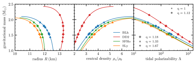
Figure 1: TOV sequences for the NS EOS used in this work. Left panel: gravitational mass versus radius. Central panel: gravitational mass versus central density normalised to the nuclear saturation density, $\rho_{0}=2.67\times 10^{14}\;{\mathrm{g}}~{}{\mathrm{c}m}^{-3}$. Right panel: gravitational mass versus tidal polarizability $\Lambda$. The different markers refer to the different mass ratios of the binaries evolved in the simulations.

We evolve BNS systems in full general relativity (GR) through 3+1 numerical relativity simulations encompassing the latest orbits, the merger and the early post-merger phase. The spacetime metric is evolved with the Z4c formulation of Einstein’s equations (Bernuzzi & Hilditch, 2010; Hilditch et al., 2013) using the CTGamma code (Pollney et al., 2011; Reisswig et al., 2013a), developed within the EinsteinToolkit framework (Loffler et al., 2012; Brandt et al., 2021). We use the WhiskyTHC code (Radice & Rezzolla, 2012; Radice et al., 2014), implemented within the Cactus (Goodale et al., 2003; Schnetter et al., 2007) framework to solve the GR hydrodynamic equations. WhiskyTHC evolves the proton and neutron number density equations, in addition to the relativistic version of the momentum and energy conservation equations, written in conservative form. To properly resolve the NS structure and merger dynamics, and at the same time track the evolution of the ejecta on a large enough domain, we employ a mesh refinement (Schnetter et al., 2004; Reisswig et al., 2013b) consisting in seven nested grids characterised by a 1:2 linear scaling between consecutive grids, with the most refined level covering the two NSs during the inspiral and the central remnant after merger. We characterise each simulation by the resolution of the innermost grid, $h$, and in particular $h\approx 246\;{\mathrm{m}}$ for low resolution (LR) and $h\approx 185\;\mathrm{m}$ for standard resolution (SR) runs. Once the symmetry along the $z=0$ plane is taken into account, the simulated space is a cube of side $3024\;\mathrm{k}m$. For further details on the numerical setup we refer to Radice et al. (2018b). Thanks to the use of a puncture gauge, the spacetime evolution can handle the formation of a singularity within the computational domain (Thierfelder et al., 2011; Dietrich & Bernuzzi, 2015). The apparent horizon (AH) can possibly be detected by the AHFinderDirect thorn (Thornburg, 2004) of the EinsteinToolkit, from which the BH properties can be extracted.

In all simulations we include compositional and energy changes due to the emission and absorption of neutrinos of all flavours. In particular, a grey leakage scheme (Ruffert et al., 1996; Neilsen et al., 2014; Galeazzi et al., 2013) is used to model the net neutrino emission rates both from optically thick regions, where neutrinos are expected to form a diffusing gas in thermal and weak equilibrium with matter, and optically thin regions. Neutrinos are then transported by an M0 scheme (Radice et al., 2018b) through optically thin regions, where the reabsorption of streaming electron flavours (anti)neutrinos can happen in addition to local emission.

We use four finite-temperature, composition-dependent EOS compatible with current astrophysical (Cromartie et al., 2019; Miller et al., 2019; Riley et al., 2019) and nuclear (Capano et al., 2020; Jiang et al., 2020) constraints: BLh (Bombaci & Logoteta, 2018; Logoteta et al., 2021), HS(DD2) (Typel et al., 2010; Hempel & Schaffner-Bielich, 2010), SFHo (Steiner et al., 2013) and SRO(SLy4) (Douchin & Haensel, 2001; Schneider et al., 2017). In the following, we will refer to the second and fourth ones simply as DD2 and SLy4. All these EOS include neutrons, protons, nuclei, electrons, positrons, and photons as relevant thermodynamics degrees of freedom, and assume baryon matter in nuclear statistical equilibrium. The BLh EOS Logoteta et al. (2021) is an extension of the zero-temperature BL EOS Bombaci & Logoteta (2018) that includes finite-temperature effects and arbitrary particle composition. It was obtained within the finite-temperature version of the Brueckner–Bethe–Goldstone quantum many-body theory in the Brueckner–Hartree–Fock approximation. The underlying two-body and three-body interactions have been derived in chiral perturbation theory taking into account the effect of nucleon-nucleon and nucleon-nucleon-nucleon interactions. DD2 and SFHo were computed in the framework of relativistic mean field theories. The two EOS differ because of the different parameterizations and coupling constants for modelling the mean-field nuclear interactions. The transition to inhomogeneous nuclear matter was done using an excluded volume approach. The SLy4 used in the present work is the finite temperature extension of the Skyrme effective nuclear interactions introduced in Douchin & Haensel (2001). The SLy4 EOS reproduces well empirical saturation properties of nuclear matter as well as several observables deduced from the mass of finite nuclei. In Fig. 1 we show the mass-radius, the mass-central density and the mass-quadrupolar tidal polarizability relations computed for the equilibrium NS sequences for the different EOS used in this work. The quadrupolar tidal polarizability is computed as $\Lambda=(2/3)k_{2}C^{-5}$, where $k_{2}$ is the dimensionless quadrupolar Love numbers (Damour, 1983; Hinderer, 2008), and $C$ the stellar compactness $C=GM/(c^{2}R)$. The SLy EOS produces the most compact NSs, while NSs modelled with the DD2 EOS have the largest radii around 13km for $1\mathrm{\,M_{\odot}}\lesssim M\lesssim 2.1\mathrm{\,M_{\odot}}$.

Initial data for our simulations are constructed using the pseudo spectral elliptic solver Lorene (Gourgoulhon et al., 2001), using the EOS slice at the lowest available temperature and assuming neutrino-less beta-equilibrium. All simulations are initialised as irrotational binaries on quasicirular orbits of coordinate radius $45\;{\mathrm{k}m}$. The residual initial eccentricity, estimated following Kyutoku et al. (2014), is between 0.02 and 0.06 for all models.

We set up and analyse a total of 28 simulations, 14 at SR and 14 at LR. In Table 1 we report a summary of all initial parameters characterising our simulations, in particular: the values of the individual stellar masses $M_{A,B}$ with $M_{A}>M_{B}$, the total gravitational mass $M$, the mass ratio $q\equiv M_{A}/M_{B}>1$, the total ADM mass and angular momentum of the system $M_{\mathrm{A}DM}$ and $J_{\mathrm{A}DM}$, the stellar compactness $C_{i}$ for $i=A,B$, the the tidal deformability of the binary, $\tilde{\Lambda}$, defined as:

$$\tilde{\Lambda}=\frac{16}{13}\frac{(M_{A}+12M_{B})M_{A}^{4}}{M^{5}}\,\Lambda_{A}+A\leftrightarrow B\,,$$ (1)

and the coefficients $k_{2}^{\mathrm{L}}$ as defined in equation 4 of Zappa et al. (2018), namely:

$$\kappa_{2}^{L}=6\left[\frac{(3M_{B}+M_{A})M_{A}^{4}}{M^{5}}\Lambda_{A}+A\leftrightarrow B\right]\,,$$ (2)

where the notation $(A\leftrightarrow B)$ indicates a second term identical to the first except that the indices $A$ and $B$ are exchanged. We also report the GW initial frequency $f_{\mathrm{G}W}(0)$ measured in Hertz. All BNS parameters are compatible with the ones inferred from the GW signal GW190425 (Abbott et al., 2020) using both the low- and high-spin priors, except for the ones characterised by $q=1.33$ and $q=1.67$, which are compatible only with high-spin prior.

To better characterise the binaries used in this work and their properties in relation to the different EOS, in Fig. 1 we also highlight the properties of the NSs initially forming the binaries evolved by our simulations. Note that the initial conditions span a broad range of central densities, from $2.2\rho_{0}$ to $6.0\rho_{0}$ (in terms of the nuclear saturation density $\rho_{0}=2.67\times 10^{14}\;{\mathrm{g}}~{}{\mathrm{c}m}^{-3}$) depending on the EOS and mass ratio. For the more asymmetric binaries, the central density of the heaviest NS is roughly $1.5$ times larger than the one of the lightest NS, while in the equal mass case the two identical NSs have a central density $\sim 1.2$ times larger than the one of the lightest NS in our sample. The single star tidal polarizability varies between two orders of magnitudes and, again, to asymmetric BNS corresponds two NSs with rather different tidal polarizability: a more compact and less deformable NS along with a larger and more deformable one. Interestingly, $\tilde{\Lambda}$ varies only by a few percents within the same EOS, while it changes by almost a factor of three between the SLy4 and the DD2 EOS.

2.2 GWs and remnant properties

We analyse the GW signal of the BNS mergers as extracted at a coordinate radius of $\approx 591\;\mathrm{k}m$ from the BNS centre of mass for all the simulations in the present work. We simulate the last 3 to 4 orbits before merger. The latter is defined as the moment in retarded time at which the amplitude of the $l=m=2$ mode of the GW waveform reaches its maximum. The short inspiral phase and the prompt collapse of the remnant to a BH do not permit to test in detail inspiral-merger-post-merger waveform models. Instead, we focus on the characterisation of the GW emission during the inspiral, merger and post-merger phases through integrated and peak quantities. In particular, we define the rescaled total energy radiated in GWs, $e_{\mathrm{G}W}^{\mathrm{t}ot}$, and the rescaled angular momentum of the remnant, $j_{\mathrm{r}em}$, as:

$$e_{\mathrm{G}W}^{\mathrm{t}ot}=\frac{(M-M_{\mathrm{A}DM})c^{2}+E_{\mathrm{G}W}^{\mathrm{r}ad}}{\nu Mc^{2}}\,,$$ (3)

and

$$j_{\mathrm{r}em}=\frac{J_{\mathrm{A}DM}-J_{\mathrm{G}W}^{\mathrm{r}ad}}{\nu GM^{2}/c}\,,$$ (4)

where $E_{\mathrm{G}W}^{\mathrm{r}ad}$ and $J_{\mathrm{G}W}^{\mathrm{r}ad}$ are the energy and angular momentum radiated in GWs during the whole simulation, and $\nu$ is the symmetric mass-ratio, $\nu=M_{A}M_{B}/M^{2}$.

Our remnants are characterised by the presence of a central BH surrounded by an accretion disc. We extract the properties of both from our simulations. In particular, we define the disc as the portion of the remnant outside the apparent horizon whose rest mass density is smaller than $10^{13}\ {{\mathrm{g}}~{}{\mathrm{c}m}^{-3}}$, (see e.g. Shibata et al., 2017). Moreover, we express the mass of the BH as

$$M_{\mathrm{B}H}^{2}=M_{\mathrm{i}rr}^{2}+\left(\frac{cJ_{\mathrm{B}H}}{2GM_{\mathrm{i}rr}}\right)^{2}\,,$$ (5)

where $M_{\mathrm{B}H}$ and $J_{\mathrm{B}H}$ are the gravitational mass and spin of the BH, respectively, while $M_{\mathrm{i}rr}$ is the irreducible BH mass:

$$M_{\mathrm{i}rr}=\frac{c^{2}}{G}\sqrt{\frac{A_{\mathrm{H}}}{16\pi}}\,,$$ (6)

with $A_{\mathrm{H}}$ the AH area. For a Kerr-BH, the irreducible mass is a non-decreasing quantity and it coincides with the gravitational mass for non rotating BHs. In analogy with the Kerr solution, we define the dimensionless spin parameter as $a_{\mathrm{B}H}\equiv(cJ_{\mathrm{B}H})/(GM_{\mathrm{B}H}^{2})$. The AH finder is able to give an estimate of such quantities by locating the AH of the singularity, albeit it is not guaranteed that it does locate the AH with sufficient accuracy. This issue can clearly have an impact on the estimated BH properties. We compare the gravitational mass provided by the AH finder with the expected BH mass

$$M_{\mathrm{B}H}^{\text{exp}}=M_{\text{ADM}}-M_{\mathrm{d}isc}-E_{\mathrm{G}W}^{\mathrm{r}ad}/c^{2}\,,$$ (7)

where $E_{\mathrm{G}W}^{\mathrm{r}ad}$ is the total energy radiated in GWs. In the above expression, we have neglected the ejecta mass and for the disc we have considered only the rest-mass energy. Similarly, for the spin parameter we compute the expected value as:

$$a_{\mathrm{B}H}^{\mathrm{e}xp}=\frac{cJ_{\mathrm{B}H}^{\mathrm{e}xp}}{G\left(M_{\mathrm{B}H}^{\mathrm{e}xp}\right)^{2}}=\frac{c(J_{{\mathrm{A}DM}}-J_{\mathrm{G}W}^{\mathrm{r}ad}-J_{\mathrm{d}isc})}{G\left(M_{\mathrm{B}H}^{\mathrm{e}xp}\right)^{2}}\,,$$ (8)

where $J_{\mathrm{G}W}^{\mathrm{r}ad}$ is the angular momentum radiated in GWs and $J_{\mathrm{d}isc}$ is the angular momentum of the surrounding disc.

2.3 Ejecta and nucleosynthesis calculations

From each simulation we consider the dynamical ejecta as the matter that becomes unbound within the end of the simulation on the basis of the geodesic criterion, i.e., when $|u_{t}|\geq c$, where $u_{t}$ is the time-component of the four-velocity. The properties of the ejecta are determined as matter crosses a spherical detector of coordinate radius $r_{\mathrm{E}}=200G\mathrm{\,M_{\odot}}/c^{2}\approx 294\ \textrm{km}$, discretised in $N_{\theta}=51$ polar and $N_{\phi}=93$ azimuthal uniform angular bins. For the unbound matter, the speed reached at infinity is computed as $v_{\infty}=c\sqrt{1-(c/u_{t})^{2}}$.

The distribution of nuclei within the expanding ejecta is computed using the same approach and the same input data as the ones reported in Perego et al. (2022), that we briefly summarise in the following. We note that a similar approach was already used in Radice et al. (2016, 2018b); Nedora et al. (2021b), but with different input data. To obtain time-dependent yield abundances we employ SkyNet (Lippuner & Roberts, 2017), a publicly available nuclear network which computes the nucleosynthesis depending on the evolution of a given Lagrangian fluid element. We evolve several trajectories with different initial parameters, with the aim of modelling the long-term expansion of the unbound matter measured in the simulations at the detector. All the trajectories start in nuclear statistical equilibrium (NSE) from an initial temperature of $T_{0}=6.0$ GK. The corresponding initial density, $\rho_{0}\equiv\rho(s,Y_{e},T=6\,\textrm{GK})$, is determined by the NSE solver implemented in SkyNet depending on the initial values of the electron fraction $Y_{e}$ and of the specific entropy $s$. The subsequent evolution of the density is set by the expansion time-scale $\tau$, first as an exponentially decaying phase and then as a homologous expansion:

$$\rho(t)=\begin{cases}\makebox[56.9055pt]{$\rho_{0}\,e^{-t/\tau}$\hfill}\textrm{if}\ t\leq 3\tau\,,\\ \makebox[56.9055pt]{$\rho_{0}\bigg{(}\dfrac{3\tau}{et}\bigg{)}^{3}$\hfill}\textrm{if}\ t>3\tau\,.\end{cases}$$ (9)

Parametric nucleosynthesis calculations are repeated for a set of fluid elements characterised by different values of $s$, $\tau$ and $Y_{e}$, ranging on a $26\times 18\times 25$ regular grid that spans the typical conditions characterising the ejecta in compact binary mergers, i.e., $1.5\leq s\ [k_{B}\ \text{baryon}^{-1}]\leq 300$, $0.5\leq\tau\ \text{[ms]}\leq 200$ and $0.01\leq Y_{e}\leq 0.48$, approximately logarithmic in the two former parameters while linear in the latter. To compute the nucleosynthetic yields in the ejecta we take the convolution of the output given by SkyNet with the distribution of the ejecta properties extracted from the numerical simulation at $r_{\mathrm{E}}$. While $s$ and $Y_{e}$ are directly extracted from the numerical simulation, $\tau$ is computed following the procedure described in Radice et al. (2016, 2018b).

2.4 Kilonova light curves calculations

In order to compute kilonova light curves from the outcome of our simulations, we employ the multi-component anisotropic framework presented in Perego et al. (2017). In this framework, axial symmetry and symmetry with respect to the BNS orbital plane are assumed, while the polar angle $\theta$ is discretised in $N_{\theta}=30$ angular bins equally spaced in $\cos{\theta}$. The kilonova emission is then computed in a ray-by-ray fashion by summing up the photon fluxes coming from each angular slice, properly projected along the line of sight of an observer located at a polar angle $\theta_{\mathrm{v}iew}$. Inside each slice, a 1D kilonova model is used. The latter depends on the mass and (root mean square) speed of the ejecta, as well as on an effective grey opacity $\kappa$. Inside each ray, several ejecta components are considered, resulting from the expulsion of matter operated by different mechanisms, acting on different time-scales and providing distinct ejecta properties. The total luminosity is found by summing over the contributions of the different ejecta components, assuming that the energy emitted by the innermost ones is quickly reprocessed and emitted by the outermost component.

Differently from the model originally implemented in Perego et al. (2017) and later employed, for example, in Radice et al. (2018b); Radice et al. (2018a); Breschi et al. (2021); Barbieri et al. (2020, 2019, 2021), here we adopt a new semi-analytical 1D kilonova model for each angular slice that we present in the following. The model assumes a spherically symmetric and optically thick outflow with a constant average grey opacity. The outflow expands with an homologous expansion law, i.e., the density of each fluid element decreases as $t^{-3}$ while its expansion speed stays constant, starting from a few hours after merger. The kilonova emission is calculated as the combination of two contributions, one emitted at the photosphere and one coming from the optically thin layers above it. The contribution coming from the photosphere is computed starting from the semi-analytic formula for the luminosity originally proposed by Wollaeger et al. (2018) and derived from a solution of the radiative transfer equation in the diffusion approximation (Pinto & Eastman, 2000). This formula was further validated in Wu et al. (2021), where it showed a very reasonable agreement with results provided by the radiation hydrodynamics code SNEC. While the original model assumes that the whole ejecta are in optically thick conditions, an increasing fraction of it resides outside of the photosphere, becoming optically thin to thermal radiation. For this reason, the outcome of this computation is rescaled by a factor $M_{\mathrm{thick}}/M_{\mathrm{ej}}$, where $M_{\mathrm{thick}}$ is the mass of the optically thick part of the ejecta, defined as the region enclosed by the photosphere. The photospheric radius $R_{\mathrm{ph}}(t)$ is found analytically by imposing the condition $\tau_{\gamma}(R_{\mathrm{ph}})=2/3$, where $\tau_{\gamma}$ is the optical depth of the material, and by using the homologous density profile as in Wollaeger et al. (2018):

$$\rho(t,x)=\rho_{0}\left(\frac{t_{0}}{t}\right)^{3}\left(1-x^{2}\right)^{3},$$ (10)

where $\rho_{0}$ is the density at the initial time $t_{0}$ and $x=v/v_{\mathrm{m}ax}$ is the dimensionless radial variable. The photospheric temperature $T_{\mathrm{ph}}(t)$ is computed from the photospheric luminosity and radius using the Stefan-Boltzmann law. A temperature floor of $2000$ $K$ for $T_{\mathrm{ph}}(t)$ is applied in order to account for electron-ion recombination in the expanding ejecta. When $T_{\mathrm{ph}}(t)$ reaches the temperature floor, $R_{\mathrm{ph}}(t)$ is redefined using again the Stefan-Boltzmann law. Furthermore a Planckian black body spectrum is assumed at the photosphere.

The contribution to the luminosity from the thin part of the ejecta is computed by partitioning the latter into equal mass shells and by assuming that each shell with temperature $T$ emits its radioactive decay energy assuming local thermodynamics equilibrium. To characterise the temperature of the thin part of the ejecta, we adopt a temperature profile similar to the one derived in Wollaeger et al. (2018) under the assumption of radiation dominated, homologous expansion: $T(t,x)=T_{0}(x)\left(t_{\mathrm{t}r}(x)/t\right)$, where $T_{0}(x)$ is the temperature of the photosphere as it transits through the shell centred in $x$ at the time $t_{\mathrm{t}r}(x)$. The bolometric luminosity contribution from the thin region is computed by multiplying the mass of each shell by the specific heating rate.

For the nuclear heating rates powering the kilonova emission, we employ the analytic fitting formula first presented in Wu et al. (2021) and based on the results from the nucleosynthesis calculations reported in Perego et al. (2022): $\dot{\epsilon}_{\mathrm{r}}(t)=At^{-\alpha}$, where $A$ and $\alpha$ are fit parameters. The latter are interpolated from tabulated values on the same $(Y_{e},s,\tau)$ grid used for the nucleosynthesis calculations (see Sec. 2.3). A constant thermalisation efficiency $\epsilon_{\mathrm{th}}=0.5$ is employed for the thick region of the ejecta, while we construct a thermalisation efficiency profile for the thin part starting from the analytic fitting formula proposed in Barnes et al. (2016). The expression for the thermalisation efficiency profile reads:

$$\epsilon_{\mathrm{th}}(t,x)=0.36\left[\exp(-aX)+\frac{\ln(1+2bX^{d})}{2bX^{d}}\right]\,,\\$$ (11)

where $a$, $b$ and $d$ are the fitting parameters reported in Barnes et al. (2016) and interpolated from tabulated values on a grid spanning the intervals $1\times 10^{-3}M_{\odot}<M_{\mathrm{ej}}<5\times 10^{-2}M_{\odot}$ and $0.1c<v_{\mathrm{ej}}<0.3c$. In the original formulation of Barnes et al. (2016), obtained assuming $\rho(t)=\rho_{0}(t/t_{0})^{3}$, $X(t,x)=t$. Due to the use in our model of the density profile Eq. (10), we adopt $X(t,x)=t/(1-x^{2})$, instead. In this work, we consider two ejecta components: a dynamical ejecta and a disc ejecta component, both symmetric with respect to the equatorial plane and to the polar axis. Following the same procedure described in Sec. 2.3, we directly extract from the simulations the profiles of the properties of the dynamical component, namely the distributions of the ejecta mass, of the root mean square velocity at infinity, of the average electron fraction, average entropy and average density at the extraction radius, as a function of the polar angle $\theta$, averaged over the azimuthal angle $\phi$. The opacity $\kappa$ is computed by interpolating the results of the atomic calculations performed in Tanaka et al. (2020) for a wide range of the electron fraction $0.01\leq Y_{e}\leq 0.50$. Additionally, inspired by disc simulations of Wu et al. (2016), Lippuner et al. (2017), Siegel & Metzger (2017), Fernández et al. (2019), Fahlman & Fernández (2022), we assume that a fraction between $\sim 20$ and $\sim 40$ per cent of the disc mass inferred from our simulations (see Sec. 3.3) is ejected in the form of a viscosity-driven wind. We model the mass of this disc wind as uniformly distributed in $\theta$, as we do not expect preferential latitudes for the ejection. Moreover, for the disc ejecta we assume a root mean square velocity of $0.06c$, a uniform opacity of $5$ ${\mathrm{c}m^{2}~{}g^{-1}}$, an average entropy of $20$ $k_{\mathrm{B}}~{}{\mathrm{b}aryon^{-1}}$ and an expansion time-scale of $30$ ms. We stress that our kilonova model relies on a large number of assumptions and simplifications which limit its accuracy. However, for the parameters that are not directly fixed by our simulations, we chose representative values in broad agreement with what obtained by fitting AT2017gfo data with the original kilonova model (Perego et al., 2017).

3 Results

3.1 Merger Dynamics

All simulations in our sample follow a qualitative common evolution pattern with quantitative differences, mainly due to the different tidal deformability provided by the EOS and BNS mass ratios. All simulations result in the prompt collapse of the central part of the remnant into a BH. In this context, we say that a BNS simulation has resulted in a prompt collapse if the minimum of the lapse function inside the computational domain decreases monotonically immediately after merger without showing core bounces. We define the moment of formation of the BH as the time at which the lapse function drops below $0.2$. In all simulations presented here the BH forms within a fraction of a ms after the merger ($t_{\mathrm{B}H}<0.47~{}{\mathrm{m}s}$, see Table 2).

Tidal forces deform the NSs during the inspiral, especially the lighter and less compact one. This effect is more pronounced for BNS with stiffer EOS, providing, for the same gravitational mass, a less compact NS. The subsequent merger dynamics is able to unbind matter from the tidal tails on a few dynamical time-scales. The neutron-rich matter ballistically expelled during this phase from the tidal tails has low entropy and can have large enough velocity to escape the potential barrier, contributing to the dynamical ejecta. The otherwise gravitationally bound matter forms a disc with toroidal shape around the forming BH. BNS models characterised by a stiffer EOS expel more matter, such that more dynamical ejecta and larger discs are found, as discussed in detail below.

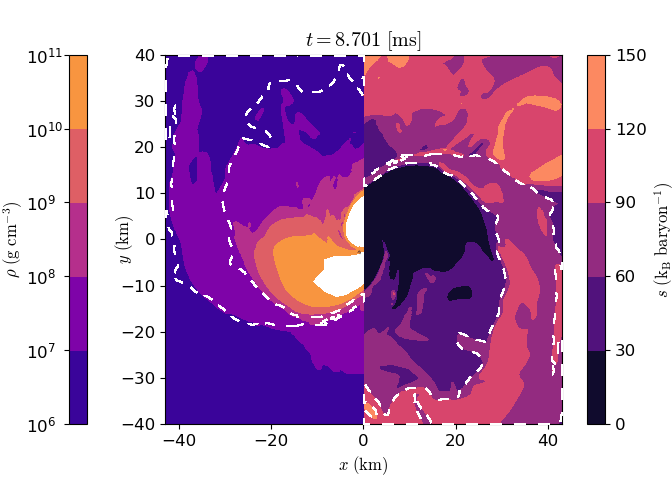
Figure 2: Snapshot of the rest mass density (left) and the entropy per baryon (right) taken at $\sim 0.3~{}{\mathrm{m}s}$ after BH formation across the orbital plane for the equal mass BNS merger SR simulation with the SFHo EOS. Matter inside the dashed contour with entropy $90-120~{}{\mathrm{k}}_{\mathrm{B}}~{}{\mathrm{b}aryon}^{-1}$ and densities $<10^{8}~{}{\mathrm{g}}~{}{\mathrm{c}m}^{-3}$ comes from the rotationally non-symmetric central object, expelled from the contact surface of the two stars. Since equal mass binaries eject few $10^{-5}~{}\mathrm{\,M_{\odot}}$, this shocked matter have a prominent role in the median properties of the ejecta.

During the few fractions of ms that precede BH formation, a small amount of very high-entropy matter coming from the NS contact interface is expelled, see Fig. 2. This extremely shocked matter is characterised by higher entropy and electron fraction than the ones that characterise matter expelled by tidal forces. This small component with entropy of $90-120~{}\mathrm{k_{B}}~{}\mathrm{baryon^{-1}}$ is responsible of the bimodal distribution of the entropy shown in Fig. 7. Its unbound component contributes to the dynamical ejecta, while the bound mass contributes to the disc formation, spanning in both cases a broader polar angle than the bound and unbound matter of tidal origin. The resulting disc, ejecta and the central BH will be the focus of Sec. 3.3 and Sec. 3.4.

3.2 Gravitational-Wave Luminosity

Table 2: For each simulation the table reports the rescaled angular momentum of the remnant, $j_{\mathrm{r}em}$; the rescaled total energy radiated in GWs, $e_{\mathrm{G}W}^{\mathrm{t}ot}$; the BH expected mass (spin), $M_{\mathrm{B}H}^{\mathrm{e}xp}$ ($a_{\mathrm{B}H}^{\mathrm{e}xp}$) as defined in Eq. (7) (Eq. (8)); the BH mass (spin) as detected from the AH finder, $M_{\mathrm{B}H}$ ($a_{\mathrm{B}H}$), together with the related average on a sample time, $\langle M_{\mathrm{H}B}\rangle$ ($\langle a_{\mathrm{B}H}\rangle$). We report values from the SR simulations and the error inside brackets estimated as the absolute semi-difference between the SR and LR values. Uncertainties refers to the least significant digit(s).

EOS	$q$	AH finder	$t_{\mathrm{B}H}-t_{\mathrm{m}rg}$	$j_{\mathrm{r}em}$	$e_{\mathrm{G}W}^{\mathrm{t}ot}$	$L_{\mathrm{p}eak}$	$M_{\mathrm{B}H}^{\mathrm{e}xp}$	$M_{\mathrm{B}H}$	$\langle M_{\mathrm{B}H}\rangle$	$a_{\mathrm{B}H}^{\mathrm{e}xp}$	$a_{\mathrm{B}H}$	$\langle a_{\mathrm{B}H}\rangle$
			(ms)			$10^{55}~{}[{\mathrm{e}rg}~{}{\mathrm{s}}^{-1}]$	$[M_{\odot}]$	$[M_{\odot}]$	$[M_{\odot}]$
BLh	1.0	✓	0.185 (2)	2.994 (8)	0.099 (1)	8.23 (13)	3.2259 (2)	3.2349 (2)	3.245 (2)	0.788 (2)	0.7860 (1)	0.801 (2)
BLh	1.12	✓	0.209 (2)	3.012 (8)	0.097 (1)	7.75 (22)	3.2250 (5)	3.2330 ($<10^{-1}$)	3.245 (2)	0.789 (2)	0.7865 (3)	0.802 (2)
BLh	1.18	✓	0.209 (30)	3.020 (6)	0.098 (1)	7.19 (9)	3.2411 (18)	3.2458 (4)	3.259 (2)	0.789 (2)	0.7866 (1)	0.803 (3)
BLh	1.33	✓	0.221 (8)	3.067 (6)	0.090 (1)	5.53 (8)	3.2559 (2)	3.2573 (6)	3.273 (1)	0.780 (5)	0.7779 ($<10^{-1}$)	0.796 (3)
DD2	1.0	✗	0.422 (10)	3.122 (9)	0.092 (2)	5.46 (18)	3.2210	-	-	0.826	-	-
DD2	1.18	✗	0.445 (6)	3.117 (6)	0.091 (1)	4.96 (12)	3.2298	-	-	0.820	-	-
DD2	1.33	✗	0.469 (41)	3.149 (2)	0.0877 (2)	4.06 (3)	3.2315	-	-	0.780	-	-
DD2	1.67	✗	0.374 (2)	3.204 (3)	0.077 (3)	2.89 (4)	-	-	-	-	-	-
SFHo	1.0	✓	0.138 (2)	2.953 (14)	0.102 (1)	9.98 (22)	3.223 (1)	3.25	3.26	0.778 (1)	0.774	0.79
SFHo	1.18	✓	0.138 (18)	2.976 (8)	0.097 (1)	8.86 (17)	3.240 (1)	3.27	3.28	0.776 (2)	0.775	0.79
SFHo	1.33	✓	0.126 (8)	3.066 (17)	0.0872 (4)	7.32 (16)	3.268	3.29	3.29	0.783	0.770	0.79
SLy4	1.0	✗	0.138 (18)	3.031 (6)	0.105 (1)	10.90 (32)	3.2167 (1)	-	-	0.801 (2)	-	-
SLy4	1.18	✗	0.114 (14)	3.010 (12)	0.103 (1)	9.67 (23)	3.2323 (6)	-	-	0.791 (3)	-	-
SLy4	1.33	✗	0.114 (2)	3.043 (9)	0.097 (1)	7.97 (7)	-	-	-	-	-	-

In the left columns of Table 2, we report GW data (i.e., $j_{\mathrm{r}em}$, $e_{\mathrm{G}W}^{\mathrm{t}ot}$, and $L_{\mathrm{p}eak}$ ) as extracted from our GW190425-like BNS simulations. We first test the quasi-universal relation between $e_{\mathrm{G}W}^{\mathrm{t}ot}$ and $j_{\mathrm{r}em}$ given in Zappa et al. (2018): $e_{\mathrm{f}it}^{\mathrm{t}ot}(j_{\mathrm{r}em})=c_{2}j_{\mathrm{r}em}^{2}+c_{1}j_{\mathrm{r}em}+c_{0}$, with $c_{0}=0.95$, $c_{1}=-0.44$ and $c_{2}=0.053$ . These coefficients were fitted over a dataset containing more than 200 BNS merger simulations performed with the BAM (Brügmann et al., 2008) and THC codes. The BNS simulations were grouped in four categories according to the fate of the remnant: prompt collapse to a BH, short-lived hypermassive NS, supramassive NS and stable NS. This simple quadratic polynomial in $j_{\mathrm{r}em}$ was very effective in relating the angular momentum of the remnant with the total radiated energy in the whole dataset, despite the different fates of the remnants, nuclear EOS, and intrinsic BNS parameters. Moreover, the ranges $j_{\mathrm{r}em}\in[2.944,3.204]$ and $e_{\mathrm{G}W}^{\mathrm{t}ot}\in[0.077,0.105]$ are compatible with the respective ranges presented in Zappa et al. (2018) for the case of BNS resulting in a prompt collapse. We notice that the absolute value of the relative error $\left|e_{\mathrm{f}it}^{\mathrm{t}ot}-e_{\mathrm{G}W}^{\mathrm{t}ot}\right|/e_{\mathrm{G}W}^{\mathrm{t}ot}$ $\lesssim\mathcal{O}(0.1)$ is in accordance with the residuals plotted in figure 4 of Zappa et al. (2018). Additionally, we remark that $e_{\mathrm{G}W}^{\mathrm{t}ot}<e_{\mathrm{G}W}^{\mathrm{f}it}$, also in accordance with the behaviour of the prompt-collapse simulations in Zappa et al. (2018). To further test the quality of the fit results with respect to the uncertainties of numerical origin we compute the ratio between the residuals and the estimated total error due to resolution uncertainties, $\sqrt{{\delta e_{\mathrm{G}W}^{\mathrm{t}ot}}^{2}+\delta{e_{\mathrm{f}it}^{\mathrm{t}ot}}^{2}}$, where $\delta e_{\mathrm{f}it}^{\mathrm{t}ot}=\sqrt{4c_{2}^{2}j_{\mathrm{r}em}^{2}+c_{1}^{2}}~{}\delta j_{\mathrm{r}em}$. The uncertainties of numerical origin, $\delta j_{\mathrm{r}em}$ and $\delta e_{\mathrm{G}W}^{\mathrm{t}ot}$, are computed as the absolute value of the semi-difference between SR and LR results. The typical values are $\lesssim 1$, indicating that the numerical error accounts for a significant fraction of the observed discrepancy. Finally we emphasise that the rescaled GW peak luminosity, $(q/\nu)^{2}\,L_{\mathrm{p}eak}$, and $\kappa_{2}^{L}$ coefficient span the same range of the prompt collapse BNSs reported in figure 2 of Zappa et al. (2018), i.e., $[1.11,2.36]\times 10^{58}~{}{\mathrm{e}rg}~{}{\mathrm{s}}^{-1}$ and $[134,387]$, respectively. We recall that $\kappa_{2}^{L}$ is the coefficient that parametrises the leading effect of tides on the GW emission from a BNS merger in the post-Newtonian expansion, Eq. (2).

3.3 Remnant Properties

Remnants in our simulations are characterised by a light accretion disc surrounding a spinning BH formed $\lesssim 0.5~{}\mathrm{m}s$ after the merger. In the following we present the properties of both as extracted from our simulations.

3.3.1 Accretion disc

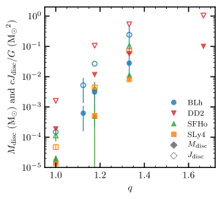
Figure 3: Disc mass (filled markers) and angular momentum (empty markers) at $4-7$ ms after merger for SR simulations. Mass and angular momentum increase with the mass ratio. The trends suggest a link between mass and angular momentum since $cJ_{\mathrm{d}isc}/G\sim(8-10)M_{\odot}\,M_{\mathrm{d}isc}$. Errors are estimated as $|{\mathrm{S}R}-{\mathrm{L}R}|$ when the LR is available.

During the last few orbits, the disc starts to form because of the tidal interaction between the two stars. In high-mass binaries resulting in prompt BH formation, the tidal interaction that occurs before and at merger is the major source of the disc. A few ms after merger the disc mass and angular momentum reach a quasi-steady phase, and slowly decrease until the end of the simulation.

In Fig. 3, we report the mass (filled markers) and angular momentum (unfilled markers) of the discs once they have reached their quasi-steady phase (i.e. $\sim 5-7$ ms after merger), computed as the integral of mass and angular momentum densities extracted from our simulations. The masses (angular momenta) span a broad range from $\sim 10^{-5}\mathrm{\,M_{\odot}}$ to $0.1\mathrm{\,M_{\odot}}$ $(10^{-4}\;-\;1\;\mathrm{\,M_{\odot}}^{2})$ depending on the BNS parameters. Both the disc mass and angular momentum increase as a function of the mass ratio $q$. We find that the increase is more pronounced for stiffer EOS, where the tidal interaction is more efficient due to the larger $\tilde{\Lambda}$. For example, considering the trend for fixed $q=1.33$, the DD2 simulation ($\tilde{\Lambda}=254$) leads to the formation of a disc twice more massive than the one formed in the BLh simulation ($\tilde{\Lambda}=135$) and roughly six times more massive than those in the SFHo ($\tilde{\Lambda}=105$) and SLy4 ($\tilde{\Lambda}=93$) simulations. The errors on the disc mass, estimated when both resolutions are available as the absolute semi-difference between the SR and LR are in the range 25-40 per cent for very light discs and get smaller ($\sim 3$ per cent) as the disc mass increases above $10^{-3}\mathrm{\,M_{\odot}}$. Resolution effects are higher for the BLh simulation with $q=1.18$, for which the disc mass of the LR simulation is $\sim 14$ times larger than the SR one. Despite efforts, we did not find the origin of such difference.

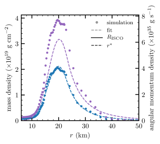
Figure 4: Disc’s radial density (blue points, left $y$-axis) and radial angular momentum density (purple points, right $y$-axis) for the BNS with BLh EOS and $q=1.33$. The blue dashed line is $\sigma(r)$ fitted on the numerical data, while the purple dashed line is the corresponding Keplerian angular momentum density. The vertical dashed line is the boundary between the Gaussian and the power-law $r^{*}$ in Eq. (12). The vertical solid line is $R_{\mathrm{I}SCO}$.

Fig. 3 suggests a correlation between the mass and the angular momentum of the disc, i.e., $J_{\mathrm{d}isc}\sim(8-10)M_{\odot}\,GM_{\mathrm{d}isc}/c$, possibly independent from the EOS and mass ratio. Stated differently, the mean specific angular momentum of the disc is (roughly) constant: $J_{\mathrm{d}isc}/M_{\mathrm{d}isc}\sim(8-10)M_{\odot}\,G/c$.

To provide a possible explanation, we consider the radial density distributions, $\sigma(r)=\int d\phi dz~{}\rho(r,\phi,z)$, as obtained from our numerical simulations, and we approximate it with a Gaussian peak smoothly connected to a radial power-law:

$$\sigma(r)=\begin{cases}b\exp\left(-\dfrac{(r-r_{\mathrm{p}eak})^{2}}{2s^{2}}\right)&0\leq r\leq r^{*}\\ \sigma_{0}\left(\dfrac{r}{r^{*}}\right)^{-\alpha}&r>r^{*}\end{cases}$$ (12)

where $b$, $r_{\mathrm{p}eak}$, $s$ and $\alpha$ are fitted against the actual radial density distribution in our simulations, while $\sigma_{0}$ and $r^{*}$ are fixed requiring $\sigma(r)$ to be differentiable in $r^{*}$. The parameter values and the quality of the fit are described in Appendix A. Additionally, we assume a Keplerian angular velocity profile, $\omega_{\mathrm{k}ep}(r)=\sqrt{GM_{\mathrm{B}H}/r^{3}}$, inside the disc. The mass and angular momentum of the resulting Keplerian disc are:

$$M_{\mathrm{d}isc}^{\mathrm{k}ep}=\int_{0}^{\infty}r\sigma(r){\mathrm{d}}r, J_{\mathrm{d}isc}^{\mathrm{k}ep}=\int_{0}^{\infty}r^{3}\sigma(r)\,\omega_{\mathrm{k}ep}(r){\mathrm{d}}r.$$ (13)

In Fig. 4, we show the result of the fit for $\sigma(r)$ (blue dashed line) on the numerical one (blue dots) for the simulation with the BLh EOS and $q=1.33$. We also show the radial angular momentum density from the numerical simulation (purple points) and the corresponding Keplerian analogue computed from Eq. (13) with the fitted $\sigma(r)$ (purple dashed line). We found that $J_{\mathrm{d}isc}^{\mathrm{k}ep}\lesssim J_{\mathrm{d}isc}$, usually within $30$ per cent over more than two orders of magnitudes in $J_{\mathrm{d}isc}$. We excluded the discs of equal mass BNS from this analysis since they are very light and $40-100$ per cent of their mass is inside the innermost stable circular orbit (ISCO) predicted according to the BH properties. Such discs will be accreted by the BH on the viscous timescale. Given Eqs. (12)-(13), the ratio between $J_{\mathrm{d}isc}^{\mathrm{k}ep}$ and $M_{\mathrm{d}isc}^{\mathrm{k}ep}$ can be written as (see Appendix A for a derivation):

$$\frac{J^{\mathrm{k}ep}_{\mathrm{d}isc}}{M^{\mathrm{k}ep}_{\mathrm{d}isc}}=\left(\eta\,\frac{\alpha-2}{\alpha-5/2}\sqrt{\frac{M_{\mathrm{B}H}}{\mathrm{\,M_{\odot}}}\frac{2r^{*}}{R^{\mathrm{S}ch}_{\odot}}}\right)~{}\frac{G\mathrm{\,M_{\odot}}}{c}\,,$$ (14)

where $\eta$ is defined as in Eq. (23) and varies between 0.78 and 0.90 with average $0.83$ in our numerical simulations, $R_{\odot}^{\mathrm{S}ch}$ is the Schwarzschild radius of the Sun, $r^{*}$ is such that $21{\mathrm{k}m}\lesssim r^{*}\lesssim 40{\mathrm{k}m}$, while $M_{\mathrm{B}H}\approx 3.21-3.26\mathrm{\,M_{\odot}}$ (see Sec. 3.3.2). The parameter which is subject to more significant variation is $\alpha\in[4.0,13.9]$ whose average is $7.5$ (see Appendix A for the values of $\alpha$ and $r^{*}$). Inserting these ranges of values in Eq. (14), one obtains $J^{\mathrm{k}ep}_{\mathrm{d}isc}/M^{\mathrm{k}ep}_{\mathrm{d}isc}\sim 6-9~{}\mathrm{\,M_{\odot}}$ with average of $7.3~{}\mathrm{\,M_{\odot}}$, in agreement within $\approx 83$ per cent with the average $\langle J_{\mathrm{d}isc}/M_{\mathrm{d}isc}\rangle=8.8~{}\mathrm{\,M_{\odot}}$ obtained by our numerical simulations.

3.3.2 Black hole

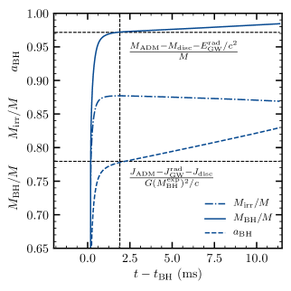
Figure 5: Evolution of the normalised BH irreducible mass $M_{\mathrm{i}rr}/M$, gravitational mass $M_{\mathrm{B}H}/M$ and dimensionless spin parameter $a_{\mathrm{B}H}$ for a SR simulation based on the BLh EOS with $q=1.33$. Horizontal dashed lines represent the expected values for the gravitational mass $(M_{\mathrm{A}DM}-E_{\mathrm{G}W}^{\mathrm{r}ad}-M_{\mathrm{d}isc})/M$ and the spin parameter $(J_{\mathrm{A}DM}-J_{\mathrm{G}W}^{\mathrm{r}ad}-J_{\mathrm{d}isc})/(M_{\mathrm{B}H}^{\mathrm{e}xp})^{2}$. Vertical dashed lines indicate the time at which the irreducible mass starts to decrease and the corresponding value on the plotted line.

In Fig. 5 we report the BH irreducible and gravitational masses, and the dimensionless spin parameter as a function of time after the BH formation for the BLh simulation at SR with $q=1.33$. We see that all the three quantities increase abruptly as the AH finder detects the apparent horizon. The horizontal dashed lines indicate the expected values $M^{\mathrm{e}xp}_{\mathrm{B}H}$ and $a^{\mathrm{e}xp}_{\mathrm{B}H}$, while the vertical dashed line indicates the time at which the irreducible mass reaches its maximum value (a few ms after the BH formation). Although $M_{\mathrm{i}rr}$ is expected to remain constant or to increase, we find that after having reached the maximum it starts to slowly decrease. We attribute this behaviour to numerical and discretisation errors in tracing the AH location. While the AH shrinks, $M_{\mathrm{B}H}$ and $a_{\mathrm{B}H}$ continue to increase without reaching saturation. Matter accretion from the disc is not sufficient to explain this growth. The rise of $M_{\mathrm{B}H}$ after the maximum of $M_{\mathrm{i}rr}$ is due to the continuous increase of the BH spin, which is an artefact of our simulations. Due to these uncertainties, we decide to focus on the gravitational mass and spin parameter of the BH at the moment when the irreducible mass is maximum.

In Table 2 we report the gravitational mass $M_{\mathrm{B}H}$ and the spin parameter $a_{\mathrm{B}H}$ of the BH computed on the basis of the latter definition. To give more conservative values of the BH properties, we report also the time averages of the BH mass, $\langle M_{\mathrm{B}H}\rangle$, and spin parameter, $\langle a_{\mathrm{B}H}\rangle$, over the first $7~{}\mathrm{m}s$ after the time at which $M_{\mathrm{i}rr}$ is maximum. We report the available data obtained by SR simulations and we estimate the uncertainties (when available) as the semi-difference with respect to the data from the corresponding LR simulations when available. In the case of simulations employing the BLh or SFHo EOS, the AH is resolved by the AH finder and the BH properties can be analysed with appropriate accuracy. More quantitatively, $M_{\mathrm{B}H}$ and $a_{\mathrm{B}H}$ differ from the respective expected values less than 1 per cent. On the other hand, the AH finder was unable to detect the AH for the simulations employing the DD2 or SLy4 EOS. In these cases we decided not to report the corresponding values in Table 2.

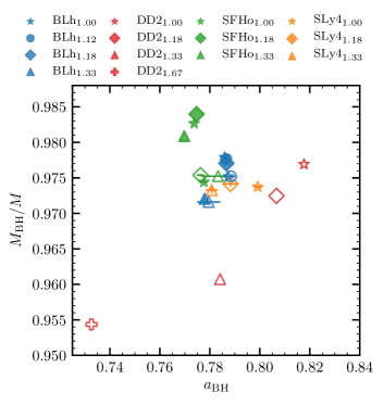
Figure 6: $M_{\mathrm{B}H}/M$ and dimensionless spin parameter $a_{{\mathrm{B}H}}$ distribution for the SR simulations of this work. Filled markers represent the values computed by the AH finder, while empty markers represent the expected ones. Errors are computed as the absolute semi-difference between SR and LR when available. For the filled markers errors are smaller than the symbol size.

Regarding the dependence of the BH properties on the initial binary parameters, the final outcome depends mostly on two effects. On one hand, energy and angular momentum are extracted from the central object via the ejection of matter and the formation of a remnant disc. On the other hand, GWs carry energy and angular momentum away. Both these effects reduce at the same time $M_{\mathrm{B}H}$ and $J_{\mathrm{B}H}$. Since $J_{\mathrm{d}isc}\approx 10~{}\mathrm{\,M_{\odot}}~{}G/c~{}M_{\mathrm{d}isc}$, the formation of a massive disc is particularly efficient in reducing the BH angular momentum, and ultimately also the spin parameter since the variation of $a_{\mathrm{B}H}^{\mathrm{e}xp}$ due to the disc formation only becomes $\left.\delta a_{\mathrm{B}H}^{\mathrm{e}xp}\right|_{\mathrm{d}isc}\approx(2a_{\mathrm{B}H}^{\mathrm{e}xp}-10\mathrm{\,M_{\odot}}/M_{\mathrm{B}H}^{\mathrm{e}xp})\delta M_{\mathrm{d}isc}/M_{\mathrm{B}H}^{\mathrm{e}xp}\sim-0.468~{}\delta M_{\mathrm{d}isc}/(\mathrm{\,M_{\odot}})$. As visible in Fig. 6, (quasi) equal mass binary simulations employing the DD2 EOS have the largest spin parameters, since their symmetric character produces a smaller disc mass, while their larger $\kappa_{2}^{\mathrm{L}}$ implies a lower GW emission. However, very asymmetric binaries employing the same EOS produce massive discs reducing efficiently both $M_{\mathrm{B}H}$ and $a_{\mathrm{B}H}$. A similar, but less significant effect, is also observed for simulations employing the BLh and SFHo EOS. For simulations employing the SLy EOS (whose discs are usually the lightest), $a_{\mathrm{B}H}$ decreases with $q$, while $M_{\mathrm{B}H}/M$ stays roughly constant. Focusing on the (quasi-)equal mass simulations using the BLh, SFHo or SLy4 EOS, the removal of mass and angular momentum through the disc formation becomes subdominant, while the dominant process is the GW emission. More symmetric binaries modelled with the SLy4 EOS (corresponding to lower values of $\kappa_{2}^{\mathrm{L}}$), have indeed the smallest BH masses.

3.4 Dynamical Ejecta

Table 3: Dynamical ejecta properties for each simulation. $M_{\mathrm{e}j}$ is the total mass of the ejecta; $\theta_{\mathrm{e}j}^{\mathrm{S}D}$ and $\phi_{\mathrm{e}j}^{\mathrm{S}D}$ are the mass-weighted standard deviation of the polar and azimuthal angle, respectively; $v_{\infty}^{\mathrm{m}ed}$, $Y_{e}^{\mathrm{m}ed}$ and $s_{\mathrm{e}j}^{\mathrm{m}ed}$ are the median values of the electron fraction, speed and entropy distributions. The last column is the ratio $X_{s}\equiv M_{\mathrm{e}j}^{\mathrm{s}hocked}/M_{\mathrm{e}j}$, where the shocked and tidal ejecta are defined as the components with entropy respectively above and below the threshold of $10\ k_{\mathrm{B}}~{}{\mathrm{b}aryon}^{-1}$. The subscript and superscript numbers indicate the 15 and 75 percentile around the median of the respective quantity.

EOS	$q$	Resolution	$M_{\mathrm{e}j}$ $[10^{-4}{\mathrm{M}_{\odot}}]$	$\theta_{\mathrm{e}j}^{\mathrm{S}D}$	$\phi_{\mathrm{e}j}^{\mathrm{S}D}$	$v_{\infty}^{\mathrm{m}ed}$ $[c]$	$Y_{e}^{\mathrm{m}ed}$	$s_{\mathrm{e}j}^{\mathrm{m}ed}$ $[k_{\mathrm{B}}~{}{\mathrm{b}aryon}^{-1}]$	$X_{s}$
BLh	1.0	SR LR	0.002 0.023	- -	- -	- -	- -	- -	- -
BLh	1.12	SR LR	0.039 0.090	- -	- -	- -	- -	- -	- -
BLh	1.18	SR LR	0.164 0.182	21.3 23.3	82.0 89.8	$0.24^{\tiny{+0.08}}_{\tiny{-0.12}}$ $0.21^{\tiny{+0.07}}_{\tiny{-0.10}}$	$0.21^{\tiny{+0.07}}_{\tiny{-0.08}}$ $0.25^{\tiny{+0.04}}_{\tiny{-0.07}}$	$18.1^{\tiny{+39.4}}_{\tiny{-11.6}}$ $41.2^{\tiny{+55.4}}_{\tiny{-31.5}}$	0.78 0.94
BLh	1.33	SR LR	0.508 0.959	18.2 20.7	74.0 78.6	$0.27^{\tiny{+0.10}}_{\tiny{-0.14}}$ $0.29^{\tiny{+0.10}}_{\tiny{-0.15}}$	$0.17^{\tiny{+0.9}}_{\tiny{-0.5}}$ $0.16^{\tiny{+0.14}}_{\tiny{-0.5}}$	$9.71^{\tiny{+17.4}}_{\tiny{-4.21}}$ $12.3^{\tiny{+22.0}}_{\tiny{-6.87}}$	0.61 0.63
DD2	1.0	SR LR	0.586 0.416	26.3 23.8	95.1 92.1	$0.28^{\tiny{+0.09}}_{\tiny{-0.12}}$ $0.32^{\tiny{+0.06}}_{\tiny{-0.08}}$	$0.27^{\tiny{+0.04}}_{\tiny{-0.06}}$ $0.29^{\tiny{+0.03}}_{\tiny{-0.05}}$	$33.2^{\tiny{+38.8}}_{\tiny{-18.3}}$ $47.1^{\tiny{+42.4}}_{\tiny{-31.4}}$	1.00 1.00
DD2	1.18	SR LR	7.16 9.67	21.4 18.1	122 87.3	$0.27^{\tiny{+0.10}}_{\tiny{-0.14}}$ $0.27^{\tiny{+0.11}}_{\tiny{-0.15}}$	$0.17^{\tiny{+0.05}}_{\tiny{-0.06}}$ $0.19^{\tiny{+0.06}}_{\tiny{-0.08}}$	$10.28^{\tiny{+7.18}}_{\tiny{-4.12}}$ $9.36^{\tiny{+5.42}}_{\tiny{-3.80}}$	0.57 0.63
DD2	1.33	SR LR	4.00 3.94	17.3 21.7	76.6 80.7	$0.23^{\tiny{+0.08}}_{\tiny{-0.11}}$ $0.19^{\tiny{+0.10}}_{\tiny{-0.11}}$	$0.15^{\tiny{+0.05}}_{\tiny{-0.05}}$ $0.13^{\tiny{+0.8}}_{\tiny{-0.05}}$	$9.38^{\tiny{+3.64}}_{\tiny{-3.66}}$ $9.34^{\tiny{+5.15}}_{\tiny{-3.29}}$	0.65 0.52
DD2	1.67	SR LR	4.05 6.20	11.1 13.0	103 95.8	$0.20^{\tiny{+0.14}}_{\tiny{-0.14}}$ $0.13^{\tiny{+0.13}}_{\tiny{-0.8}}$	$0.10^{\tiny{+0.03}}_{\tiny{-0.07}}$ $0.06^{\tiny{+0.08}}_{\tiny{-0.03}}$	$5.66^{\tiny{+4.27}}_{\tiny{-1.87}}$ $6.15^{\tiny{+3.70}}_{\tiny{-3.33}}$	0.29 0.37
SFHo	1.0	SR LR	0.023 0.033	- -	- -	- -	- -	- -	- -
SFHo	1.18	SR LR	0.071 0.151	- 24.5	- 90.6	- $0.22^{\tiny{+0.07}}_{\tiny{-0.10}}$	- $0.26^{\tiny{+0.03}}_{\tiny{-0.04}}$	- $72.3^{\tiny{+51.3}}_{\tiny{-53.1}}$	- 0.97
SFHo	1.33	SR LR	0.603 1.87	12.7 13.1	68.8 85.0	$0.26^{\tiny{+0.10}}_{\tiny{-0.13}}$ $0.32^{\tiny{+0.10}}_{\tiny{-0.16}}$	$0.13^{\tiny{+0.04}}_{\tiny{-0.06}}$ $0.13^{\tiny{+0.05}}_{\tiny{-0.05}}$	$7.55^{\tiny{+4.97}}_{\tiny{-3.30}}$ $6.45^{\tiny{+5.08}}_{\tiny{-2.50}}$	0.37 0.32
SLy4	1.0	SR LR	0.030 0.024	- -	- -	- -	- -	- -	- -
SLy4	1.18	SR LR	0.055 0.114	- 21.4	- 79.5	- $0.22^{\tiny{+0.10}}_{\tiny{-0.10}}$	- $0.24^{\tiny{+0.05}}_{\tiny{-0.06}}$	- $38.1^{\tiny{+97.5}}_{\tiny{-31.4}}$	- 0.79
SLy4	1.33	SR LR	2.29 1.12	9.0 14.6	71.5 70.8	$0.40^{\tiny{+0.12}}_{\tiny{-0.20}}$ $0.30^{\tiny{+0.10}}_{\tiny{-0.14}}$	$0.10^{\tiny{+0.03}}_{\tiny{-0.02}}$ $0.12^{\tiny{+0.09}}_{\tiny{-0.5}}$	$5.48^{\tiny{+1.82}}_{\tiny{-3.15}}$ $7.40^{\tiny{+8.42}}_{\tiny{-4.44}}$	0.22 0.49

In Table 3, we present the properties of the dynamical ejecta as extracted from our simulations, namely the mass of the ejecta, $M_{\mathrm{e}j}$; the standard deviation (SD) of the polar ($\theta\in[0^{\circ},180^{\circ}]$) and azimuthal ($\phi\in[0^{\circ},360^{\circ}]$, see Appendix C for more details on its calculation) angular distributions, $\theta_{\mathrm{e}j}^{\mathrm{S}D}$ and $\phi_{\mathrm{e}j}^{\mathrm{S}D}$, respectively; the median of the distribution of the velocity at infinity, $v_{\infty}^{\mathrm{m}ed}$, of the electron fraction, $Y_{e}^{\mathrm{m}ed}$, and of the entropy per baryon, $s_{\mathrm{e}j}^{\mathrm{m}ed}$. The last column refers to the fraction of shocked ejecta $X_{s}$, defined as the fraction of the ejecta whose entropy is larger than $10\,k_{\mathrm{B}}~{}{\mathrm{b}aryon^{-1}}$. We report the values for both SR and LR simulations accompanied by the 15-75 percentile range around the median computed from the respective mass-weighted histogram. We do not report the ejecta properties when $M_{\mathrm{e}j}<10^{-5}\mathrm{\,M_{\odot}}$, since the properties of such a small amount of ejected matter cannot be trusted due to numerical uncertainties. Additionally, in Fig. 7, we present mass histograms of the $v_{\infty}$, $Y_{e}$, $s_{\mathrm{e}j}$ and $\theta_{\mathrm{e}j}$ distributions for simulations at SR for which $M_{\mathrm{e}j}\geq 10^{-5}\mathrm{\,M_{\odot}}$. The vertical solid (dashed) lines represent the medians (average) of the ejecta properties for the $q=1.33$ cases, taken as representative case. While the difference between mean and median is small or even negligible for the velocity and the electron fraction, a significant difference is clear in the entropy distribution.

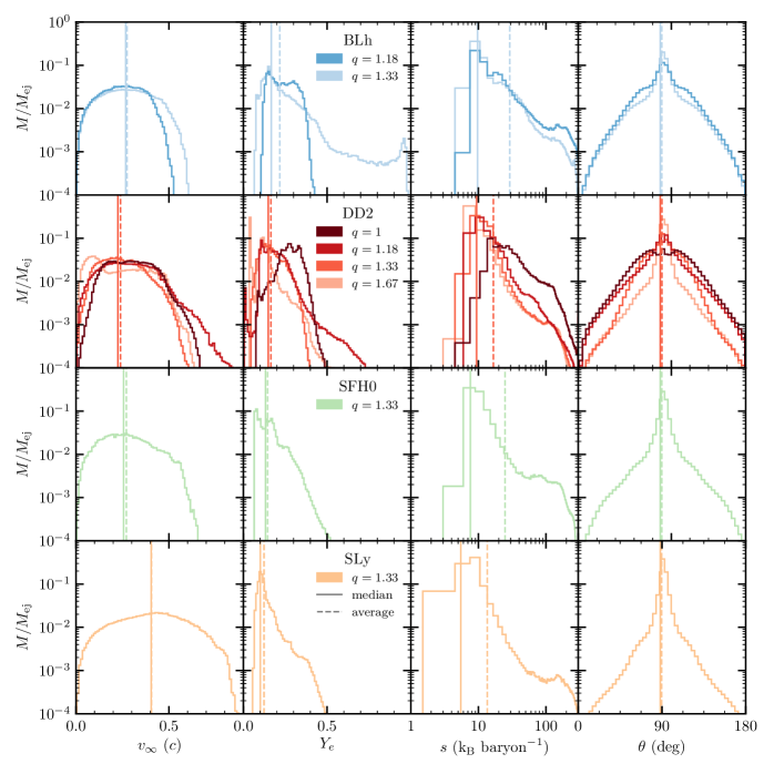
Figure 7: Histograms of the dynamical ejecta. From the first to the last column: velocity at infinity $v_{\infty}$, electron fraction $Y_{e}$, entropy per baryon $s$ and polar angle $\theta_{\mathrm{e}j}$. Each row represents a different EOS. From the first to the last line: BLh, DD2, SFHo, SLy4. As a representative case, we represent the median and the average values of all quantities for the $q=1.33$ cases as vertical solid and dashed lines, respectively. The high $Y_{e}$ tail in the BLh, $q=1.33$ case is not robust due to the finite size of the EOS tables not extending above $Y_{e}=0.6$.

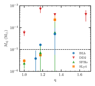
Figure 8: Dynamical ejecta mass as a function of the mass ratio $q$ of the binary. Different symbols denote numerical simulations with different EOS. Simulations with $M_{\mathrm{e}j}<10^{-6}\;\mathrm{\,M_{\odot}}$ have been excluded, while only ejecta with $M_{\mathrm{e}j}>10^{-5}\;\mathrm{\,M_{\odot}}$ is trusted due to numerical uncertainties. Errors are computed as the absolute difference between SR and LR values.

The ejecta mass ranges from values smaller than $10^{-5}\mathrm{\,M_{\odot}}$ up to $\sim 6\times 10^{-4}\mathrm{\,M_{\odot}}$, increasing with the mass ratio $q$ and the stiffness of the EOS, as visible in Fig. 8. For asymmetric systems ($q\neq 1$) and stiffer EOS, the tidal interaction is more efficient in deforming the secondary NS and the resulting merger dynamics is more effective in expelling matter from its tidal tails (see e.g. Hotokezaka et al., 2013; Bauswein et al., 2013; Sekiguchi et al., 2015; Rosswog, 2015; Lehner et al., 2016; Dietrich et al., 2017; Bernuzzi et al., 2020). Simulations employing the DD2 EOS exhibit a deviation from this trend at higher mass ratios ($q=1.33,\,1.67$), for which the value of the ejecta mass saturates or even tends to decrease, similarly to what found in Dudi et al. (2021) (see Sec. 5). We speculate that the ejection process at high $q$’s is more sensitive to usually subdominant effects, including the detailed behaviour of the NS radius and of $\tilde{\Lambda}$, see Fig. 1 and Table 1. For the latter quantity, for high-$q$ BNSs, models employing the DD2 show a decreasing $\tilde{\Lambda}$ (see Table 1). It suggest that for asymmetric enough BNS ($q\gtrsim 1.2$ in our case), if an additional increase of the asymmetry is not accompanied by and increase of $\tilde{\Lambda}$, the ejecta mass can saturate or even decrease. More simulations at higher resolutions are needed to confirm the robustness of this trend.

The SD of the geometrical angles gives an indication of the spatial distribution of the ejected matter. We find that the ejecta spread over the whole space, but it is mostly concentrated close to the equator, with an opening angle $2\theta_{\mathrm{e}j}^{\mathrm{S}D}$ that varies across the range $18^{\circ}-54^{\circ}$, depending on the binary properties and where higher values correspond to more symmetric binaries. This can be understood since the tidal interaction tends to distribute matter along the orbital plane. The SD of the azimuthal angle $\phi_{\mathrm{e}j}^{\mathrm{S}D}$ is related to the rotational symmetry of the dynamical ejecta around the orbital axis. For a mass distribution uniform in $\phi$ and centred in $180^{\circ}$ with symmetric support on $2\alpha\in[0,360^{\circ}]$, we expect a SD of $\phi_{\mathrm{e}j}^{\mathrm{S}D}=(\sqrt{3}/3)~{}\alpha\approx 52^{\circ}(\alpha/90^{\circ})$. The values of $\phi_{\mathrm{e}j}^{\mathrm{S}D}$ obtained in our simulations range within $65^{\circ}-96^{\circ}$ and are compatible with a uniform distribution centred in $180^{\circ}$ with support on $\sim 225^{\circ}-360^{\circ}$ respectively, where higher values correspond to equal-mass systems. This indicates that the dynamical ejecta expelled by symmetric binaries is distributed over the whole azimuthal angle, while the anisotropy increases with $q$ (see e.g. Bovard et al., 2017; Radice et al., 2018b; Bernuzzi et al., 2020).

The distribution of the radial velocity at infinity has $v_{\infty}^{\mathrm{m}ed}$ ranging from $\sim 0.2\,c$ to $\sim 0.4\,c$, with fast tails reaching $\sim 0.6-0.9\,c$ for the highest mass ratios. The median of the electron fraction distribution is always smaller than $0.3$ and is lower for higher mass ratios: tidal interaction ejects cold neutron rich material only marginally subject to composition reprocessing from positron and neutrino captures (e.g. Wanajo et al., 2014; Sekiguchi et al., 2015; Perego et al., 2017; Martin et al., 2018). Finally, the entropy per baryon has a distribution with a marked peak at relatively low entropy, between $\sim 5\;k_{\mathrm{B}}~{}{\mathrm{b}aryon}^{-1}$ and $\sim 20\;k_{\mathrm{B}}~{}{\mathrm{b}aryon}^{-1}$, and a slow decrease towards higher entropy, with medians that in the SR cases range between $\sim 5\;k_{\mathrm{B}}~{}{\mathrm{b}aryon}^{-1}$ and $\sim 18\;k_{\mathrm{B}}~{}{\mathrm{b}aryon}^{-1}$ (with the only exception of the $q=1$ simulation employing the DD2 EOS, and more often $\lesssim 10~{}k_{\mathrm{B}}~{}{\mathrm{b}aryon}^{-1}$). All the entropy distributions show a second peak around $s_{\mathrm{e}j}\sim 120\;k_{\mathrm{B}}~{}{\mathrm{b}aryon}^{-1}$ whose relative importance decreasing with $q$ and with the stiffness of the EOS, ranging approximately between $10^{-2}$ and $10^{-3}$. This high-entropy component reflects the presence of a shocked fraction of the ejecta coming from the collisional interface of the two NSs (see Sec. 3.1 and Fig. 2). We expect this component to be present also in BNS mergers characterised by lower total masses (and often not resulting in a prompt collapse), in which the total amount of ejected matter is typically larger than what found in our simulations. The compositional properties of the dynamical ejecta show distributions comparable to what studied in Most et al. (2021) for the case of an irrotational binary, with similar fast-tail, high ye and high entropy components.

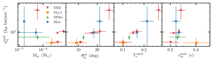
Figure 9: Correlation of the ejecta mass $M_{ej}$, standard deviation of the polar angle $\theta_{\mathrm{e}j}^{\mathrm{S}D}$, median of the electron fraction $Y_{e}^{\mathrm{m}ed}$ and median of the velocity at infinity $v_{\infty}^{\mathrm{m}ed}$ with the median of the entropy $s_{\mathrm{e}j}^{\mathrm{m}ed}$. Uncertainties are estimated as the absolute difference between SR and LR simulations, while SR values are used to represent the points. The simulations with higher mass ratios have higher values of the ejected mass.

In the analysis outlined above, we have found that many properties of the ejected matter correlate with $q$ and with the EOS stiffness. We now explicitly explore correlations among the different ejecta properties. In Fig. 9, we show $M_{\mathrm{e}j}$, $Y_{e}^{\mathrm{m}ed}$ and $\theta_{\mathrm{e}j}^{\mathrm{S}D}$ as a function of $s_{\mathrm{e}j}^{\mathrm{m}ed}$ for each BNS simulation producing more than $10^{-5}\mathrm{\,M_{\odot}}$ of dynamical ejecta. We recall that lower $s_{\mathrm{e}j}^{\mathrm{m}ed}$ correspond to higher values of $q$. In the left panel we observe that $M_{\mathrm{e}j}$ is larger for lower values of $s_{\mathrm{e}j}^{\mathrm{m}ed}$ and it is usually greater for stiffer EOS. In the two middle panels, we observe that both $\theta_{\mathrm{e}j}^{\mathrm{S}D}$ and $Y_{e}^{\mathrm{m}ed}$ increase almost linearly with the logarithm of the median of the entropy distribution. This confirms that the tidal interaction tends to distribute cold, low-entropy ejecta along the orbital plane. Only for simulations in which the shock-heated component is relevant (i.e., symmetric or nearly symmetric BNSs), the angular distribution of the ejecta departs significantly from the orbital plane, indicating that shocked matter spreads more over the solid angle. Similar results were found also for unequal-mass binaries that do not collapse promptly into a black hole. (see e.g. Bauswein et al., 2013; Lehner et al., 2016; Dietrich et al., 2017; Radice et al., 2018b; Bernuzzi et al., 2020; Nedora et al., 2021a). In the right panel, we study the correlations between the median of the entropy and the median of the velocity at infinity. In our simulations $v_{\infty}^{\mathrm{m}ed}$ decrease with $s_{\mathrm{e}j}^{\mathrm{m}ed}$, indicating that higher mass ratios result in faster ejecta, contrary to what usually found in relation to systems characterised by smaller total masses. This could be indeed a peculiar property of very massive BNSs.

4 Nucleosynthesis and kilonova

4.1 Nucleosynthesis

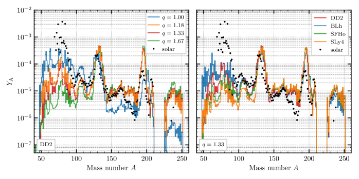
Figure 10: Nucleosynthesis pattern at $t=30$ years after the merger as a function of the mass number $A$. Left: comparison between relative abundances from simulations employing the DD2 EOS. Right: comparison between relative abundances from NR simulations with mass ratio $q=1.33$. Black dots represent the Solar $r$-process abundances, taken from Prantzos et al. (2020). To guide the comparison, the Solar residuals are scaled in order to reproduce at $A=130$ the abundance of the simulation with $q=1.33$ and the DD2 EOS.

Using the procedure outlined in Sec. 2.3, we compute nucleosynthesis yields for the dynamical ejecta of all our GW190425 targeted simulations. In Fig. 10, we present nucleosynthesis yields for a subset of representative simulations at $t=30$ years after merger, superimposed to the Solar residual $r$-process abundances taken from Prantzos et al. (2020) as a useful point of reference. To guide the comparison between the different models, the Solar residuals are scaled in order to reproduce the abundance of the simulation with $q=1.33$ and the DD2 EOS at $A=130$.

Unequal-mass merger simulations employing the DD2 EOS (left panel) robustly produce elements between the second and the third $r$-process peak, without showing any substantial difference between the various mass ratios. Relative abundances are comparable to the Solar residuals with a significant excess in the third peak height with respect to the height of the second peak, and a significant production of translead nuclei. On the other hand, $A\lesssim 120$ nuclei are systematically underproduced. A weak dependence on the value of the mass ratio is visible, with more asymmetric mergers producing on average a larger amount of heavy nuclei. These behaviours are expected given the prompt collapse of the central remnant into a BH, the tidal character of the ejection mechanism and the consequent absence of a significant high-$Y_{e}$ tail in the dynamical ejecta above a critical value $Y_{e}\gtrsim 0.22$ (e.g. Lippuner & Roberts, 2015; Radice et al., 2016), that is associated with the production of less than 10 per cent of the mass fraction of heavy nuclei above the second peak through an incomplete $r$-process.

The situation changes significantly when considering the DD2 equal-mass case (blue line). In fact, the relative abundances of heavy $r$-process nuclei ($A\gtrsim 130$ and even more for $A\gtrsim 140$) are less significant with respect to the unequal mass cases, while around the first peak the $q=1$ pattern is the largest and the closest one to the Solar abundances. This is consistent with the fact that, despite having a small total mass, the bulk of the ejecta $Y_{e}$ distribution for the equal-mass case lies within the interval $0.20-0.40$ (see Fig. 7).

The right panel of Fig. 10 shows, instead, the comparison between simulations characterised by the same mass ratio, namely $q=1.33$, but different EOS. Since the mass ratio differs significantly from 1, the nucleosynthesis outcome is in all cases similar to what described for unequal-mass merger simulations in the comparison between the DD2 simulations. All the curves are quite close to each other except around the first peak, where the spread between the various distributions becomes more evident and sensitive to the nuclear EOS, with the largest (smallest) relative values for the abundances obtained for the BLh (SLy4) EOS. Usually (and especially for equal or nearly equal mergers that do not promptly collapse to a BH), the synthesis of light $r$-process elements within BNS ejecta should be favoured by soft EOS, since the higher temperatures achieved in the shock-heated ejecta component leptonise matter in a more efficient way. However, we notice that for $A\lesssim 120$ the relative production of light $r$-process elements does not follow exactly this trend. This is because, for such asymmetric binaries promptly collapsing to BHs, the dynamical ejection of matter is usually dominated by the cold, neutron-rich tidal component. However a small, but non-negligible fraction of the dynamical ejecta comes from the contact surface of the colliding NSs and is characterised by relatively high entropies (see the $X_{\mathrm{s}}$ column in Table 3). The corresponding larger peak temperatures produce a tail in the $Y_{e}$ distribution above $\approx 0.22$. These ejecta are likely present in all BNS mergers, but their relatively low amount make them more relevant only in the case of mergers characterised by a very small dynamical ejecta mass. Moreover, these ejecta can more likely escape in the case of stiffer EOS, characterised by larger radii and less deep gravitational well.

We conclude that the nucleosynthesis patterns show a mild variability, depending on the mass ratios and EOS. However, they are comparable with the ones obtained by BNS merger simulations of lighter binary systems and do not show peculiar behaviours (see e.g. Wanajo et al., 2014; Just et al., 2015; Radice et al., 2018b; Bovard et al., 2017; Nedora et al., 2021b). Nevertheless, we point out that the nucleosynthesis yields obtained exhibit different features with respect to the Solar residuals, for example in the position and shape of the second and third $r$-process peaks. The fine structure of the abundance pattern in this region is indeed affected by the particular choice of the nuclear input data made for the nucleosynthesis calculations, like for example the nuclear mass model, the different fission channels considered (spontaneous, neutron-induced, $\beta$-delayed etc.) or the fission fragment distribution employed (see e.g. Eichler et al., 2015; de Jesús Mendoza-Temis et al., 2015; Goriely, 2015). However, since we do not expect dynamical ejecta from high-mass BNS mergers to represent the dominant contribution to the $r$-process enrichment in the Universe, possible discrepancies with the solar pattern are not an issue. In addition, one should also remember that, even for high mass BNS mergers, the nucleosynthesis from the disc ejecta is expected to dominate the dynamical ejecta one.

4.2 Kilonovae

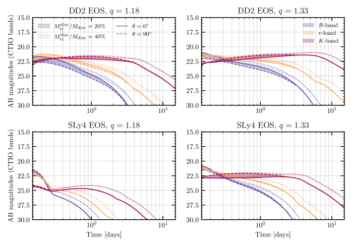
Figure 11: AB magnitudes in the blue, red and IR bands of CTIO telescope as a function of time. We report the results for the DD2 and SLy4 EOS and for a binary mass ratio of $q=1.18$ and $q=1.33$ at standard resolution. The uncertainty in the source inclination angle (varying between $0^{\circ}-90^{\circ}$) is represented using solid lines for $\theta=0^{\circ}$ and dotted lines for $\theta=90^{\circ}$, with intermediate values enclosed by the above lines. The source distance is set to $130~{}{\mathrm{M}pc}$.In each panel, the darker and lighter areas refer to two different scenarios in which $20\%$ and $40\%$ of the disc mass is expelled, respectively.

Using the model described in Sec. 2.4, we compute synthetic kilonova light curves for each of the SR models presented in this work for which the mass of the dynamical ejecta is larger than $10^{-5}\mathrm{\,M_{\odot}}$. In Fig. 11, we present the evolution of the AB magnitudes in three representative bands ($B$-, $r$-, and $K$-band), for two EOS (the stiff DD2 and the soft SLy4) and two mass ratios ($q=1.18$ and $q=1.33$). In general, kilonova magnitudes depend both on the distance and on the viewing angle. Regarding the former, the wide range of distances compatible with GW190425 ($D=70-250$ Mpc) implies a possible uncertainty of $\sim 3$ magnitudes, with lower magnitudes corresponding to shorter distances. On the other hand, the inclination angle is almost unconstrained by the GW190425 signal. Due to the degeneracy between viewing angle and distance, viewing angles close to the polar axis ($\theta_{\mathrm{v}iew}\sim 0^{\circ}$) are more compatible with larger distances, while shorter distances would imply edge-on configurations ($\theta_{\mathrm{v}iew}\sim 90^{\circ}$). In Fig. 11, we set $D=130~{}{\mathrm{M}pc}$ while we explore all possible viewing angles, $\theta_{\mathrm{v}iew}\in[0^{\circ},90^{\circ}]$. The amount of ejecta and their composition are the most relevant parameters in shaping kilonova light curves. In general, since GW190425-like events are expected to eject a relatively small amount of mass, the resulting kilonovae are predicted to be relatively dim and fast-evolving, compared for example with GW170817-like events. More specifically, in Fig. 11 we observe that the kilonova associated to the simulation employing the DD2 EOS and with $q=1.33$ is brighter and lasts longer with respect to both the simulation employing the same EOS but with $q=1.18$, and the simulation with the same mass ratio but employing the SLy4 EOS, for all bands. This mostly reflects the difference in the amount of ejecta between the different models, see Sec. 3.3 and Sec. 3.4, with greater mass ejection resulting in brighter peak luminosities due to the stronger availability of nuclear fuel required for the kilonova emission.

Differences in the viewing angle affect the light curves at times shorter than a couple of days, while our results are insensitive to the specific viewing angle at later times. This can be explained by considering that the slower and significantly more massive disc wind component, eventually powering the kilonova at late times ($t\gtrsim 1$ day), is assumed to be isotropic in our model. Conversely, within the first days after merger, the dynamical ejecta component plays a relevant role. The angular distribution of its mass and composition are thus reflected in the band magnitude evolution. In particular, we obtain brighter light curves in the visual bands at angles closer to the pole ($\theta\sim 0\degr$), where matter with a higher initial $Y_{e}$ (and thus lower opacity) can be found. Conversely, the emission in the IR band is typically brighter close to the equatorial plane ($\theta\sim 90^{\circ}$), where the most neutron-rich (and thus more opaque) matter is concentrated, with respect to higher latitudes. Since for each of our SR models the disc wind ejecta component is determinant in generating the kilonova emission, we test our results sensitivity with respect to its mass. In particular, we notice that the increase in the fraction of ejected disc mass from a plausible $20\%$ to an optimistic $40\%$ results in an overall gain in brightness of $\sim 1$ magnitude for all bands at late times, when the disc ejecta component becomes dominant. We also test the sensitivity of light curves on the disc ejecta mass and composition angular distributions. We consider a density distribution $\rho_{\mathrm{w}ind}(\theta)\propto\sin{\theta}$ as alternative to the isotropic case and an opacity distribution shaped as a step function with $k=1$ ${\mathrm{c}m^{2}~{}g^{-1}}$ for $\theta<45^{\circ}$ and $k=10$ ${\mathrm{c}m^{2}~{}g^{-1}}$ for $\theta>45^{\circ}$. While such modifications on the opacity can vary the final bolometric light curves up to a factor of a few, the different mass distribution results in a model dependence on the viewing angle also at late times. More specifically, since the wind density gradually increases towards the equator, the magnitudes decrease accordingly for all bands, and we obtain the brightest emission for $\theta_{\mathrm{v}iew}\sim 90^{\circ}$, $\sim 1$ magnitude below the polar one. Despite the non-negligible dependences, these tests place our uncertainty in the luminosity due to the disc parameters well below the one due to the source distance and viewing angle.

For simulations with $q=1.33$, providing a prominent tidal low-$Y_{e}$ ejecta component, the infrared $K$-band lasts several days and nearly always dominates over bluer bands, due to the prevailing presence of lanthanides-rich material synthesised through a strong $r$-process both in the dynamical and in the disc wind ejecta. On the other hand, in the case of the simulation with $q=1.18$ and the SLy4 EOS, the considerably lower ejecta mass with a broader $Y_{e}$ distribution results in lower material opacities and slightly brighter blue band light curves at early times.

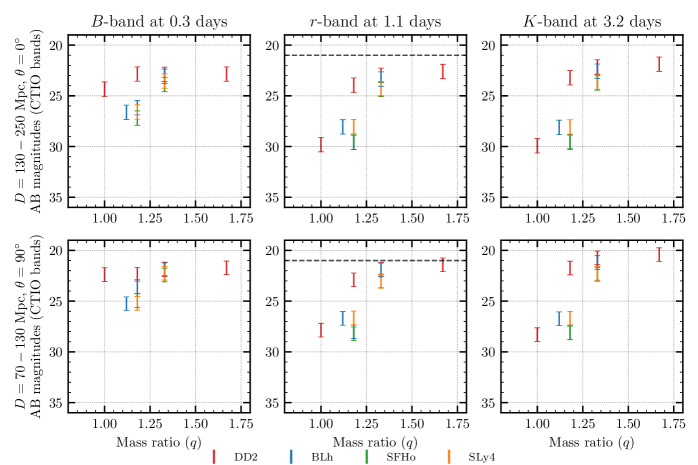
Figure 12: AB magnitudes in the blue, red and IR bands of CTIO telescope at fixed characteristic times as a function of the binary mass ratio $q$. The kilonova is obtained assuming an ejection of $20\%$ of the disc mass. Results are colour-coded to indicate different EOS. Only standard resolution simulations are shown. Two cases for the source distance and inclination angle are reported, with the error bars representing the uncertainty in the source distance. The dashed horizontal line represents the upper limit for GW190425 obtained with the ZTF by the GROWTH collaboration for the $r$ and $g$-band (Coughlin et al., 2019).

‘

Due to the evolution of the photospheric temperature, the $B$-band magnitude is the first to peak, within the very first few hours, promptly followed by the $r$-band magnitude, dominating within the first half-day after merger, while the infrared band peaks much later in time, possibly on a time-scale of days. While the precise peak times and magnitudes vary depending on the specific simulation, the presence of common trends in the light curve behaviour allow us to identify characteristic time-scales for each band in which the latter typically dominates over or is comparable to the others. In Fig. 12, we present the values of the AB magnitudes in the same three bands as in Fig. 11 at three corresponding characteristic times for each available simulation, namely at 0.3 days, 1.1 days and 3.2 days for the $B$, $r$ and $K$ band, respectively. Since we want now to address the possible detectability of GW190425, two possible ranges for the source distance and inclination angle are considered in order to account for the large degeneracy in the estimation of these parameters for GW190425 (see also Dudi et al., 2021, for a similar choice). Regardless of the specific band, magnitudes tend to decrease with the increase of the mass ratio, leading to emissions up to $\sim 8$ magnitudes brighter, moving from equal-mass to strongly asymmetric mergers. Likewise, the stiffest EOS corresponds to luminosities which can be as bright as $\sim 6$ magnitudes below the same results obtained using softer EOS. Exceptions to these trends can be directly traced back to already emerged distinctive mass ejections. For example, the simulation employing the BLh EOS and a mass ratio of $q=1.12$ returns brighter red and infrared luminosities with respect to the simulation employing the same EOS but with $q=1.18$: this is due to the fact that in the first instance the computed disc mass is greater, leading to a more massive disc wind (which dominates over the dynamical component). Based on our analysis, from Fig. 12 it is clear that almost none of our models can be fully ruled out by the ZTF upper limits to the kilonova of GW190425 (shown as a dashed horizontal line), meaning that current data cannot help further constraining the model parameters. This leaves open the question as to whether the detection of events like GW190425 can shed light on the source properties, and hints to the necessity of determining the sky localisation with high accuracy for these events, to employ deeper observations in order to resolve such EM counterparts.

5 Discussion

In this section, we compare the results of our work with recent publications about the modelling of GW190425 and of its EM counterparts, in particular with results reported in Dudi et al. (2021); Raaijmakers et al. (2021); Barbieri et al. (2021).

During the preparation of this work, Dudi et. al. published an independent study on GW190425 in NR. They used the BAM code, a NR code which was shown to produce results consistent with WhiskyTHC (see e.g. Dietrich et al., 2018). They considered four mass ratios, ranging from 1 to 1.43, and for each of them they employed three cold, beta-equilibrated EOS: the piecewise-polytropic EOS MPA1 (Read et al., 2009), a piecewise-polytropic representation of the tabulated DD2 EOS at the lowest available temperature, and the softer APR4 EOS (Akmal et al., 1998). Each model was run at three different resolutions, with our SR being intermediate between their worst and middle resolution. Similarly to what we found in our simulations, all the BNS models presented by Dudi et. al. result in a prompt collapse. Regarding the properties of the remnant, the two works predict a comparable range for $M_{\mathrm{B}H}/M$, while we notice that the dimensionless spin parameter obtained by Dudi et. al. is systematically lower than the one obtained by our simulations by several percents, corresponding to $\Delta a_{\mathrm{B}H}\sim 0.05$, when comparing simulations characterised by similar mass ratios and EOS. Both analyses agree in predicting more massive discs when considering more asymmetric binaries and stiffer EOS. In particular, the disc results for the DD2 EOS share the same trend with respect to $q$, both on a qualitative and quantitative level. Moving to the comparison of the dynamical ejecta, we first notice that the amount of matter obtained for the MPA1 and APR4 EOS by Dudi et. al. increases as the binary becomes more asymmetric, similarly to what observed in our BLh, SFHo and SLy4 simulations. Similarly, the amount of ejecta from the DD2 simulations first increases then decreases with $q$ in both analyses. However, while in the former cases the amount of ejecta are comparable among them, the values obtained for the DD2 EOS differ significantly, with the ejecta reported in Dudi et. al. larger by $\sim$ one order of magnitude. According to the reported values, uncertainties due to different resolutions seem to account only for a fraction of this discrepancy and higher resolution seems to result in smaller ejecta masses. A potentially relevant source of discrepancy could be the different microphysical input. In addition to a more accurate temperature treatment, the presence of neutrino radiation can influence the dynamical ejecta, since simulations accounting for neutrino emission show systematically smaller dynamical ejecta masses (see e.g. Nedora et al., 2022), due to the emission of neutrinos occurring during the ejection process.

The different amount of ejecta obtained employing the DD2 EOS is directly reflected in the kilonova light curves, where for a similar mass ratio the $r$-band magnitudes reported in Dudi et. al. are systematically brighter. In particular, while for edge-on views the results are in good agreement, for a viewing angle close to the polar axis we find up to $\sim 5$ magnitudes of difference between light curves corresponding to the same binary configurations. On the one hand, this may reflect the substantially different mass and composition distributions resulting from the NR models. On the other hand, we also stress that the models employed for the light curves computation are significantly different: as opposed to our semi-analytic model described in Sec. 2.4, Dudi et. al. employ a more advanced wavelength-dependent radiative transfer approach (Kawaguchi et al., 2020), for which the post-merger ejecta composition is fixed for all components. Additionally, our kilonova model decomposes the solid angle in radial slices. While this approach is reasonable for ejecta expelled over the entire solid angle, it could be inadequate for ejecta expelled only close to the equator for which it tends to underestimate magnitudes up to a few since it neglects possible lateral effects (Kawaguchi et al., 2016; Kawaguchi et al., 2018; Barbieri et al., 2019; Bernuzzi et al., 2020). Keeping in mind the above differences for the GW190425 event and working under the assumption that the location of the source was covered by ZTF, Dudi et. al. disfavored a higher number of models with respect to this work, i.e., the ones employing DD2 or MPA1 EOS with a high mass ratio and a source configuration similar to that used in the top panels of Fig. 12. On the contrary, our results imply that only the model employing the DD2 EOS with the highest mass ratio and a source distance close to $D\sim 70$ Mpc (corresponding to a edge-on view) would be disfavoured (as visible in the bottom panels of Fig. 12).

Raaijmakers et al. (2021) studied the expected photometric light curves of BNS mergers with masses in the range compatible with the posteriors of GW190425. We recall that, due to the spherical symmetry of the employed kilonova model, it was not possible to investigate the light curve dependence on the viewing angle, even if selected tests with the multidimensional POSSIS code were performed (Bulla, 2019). By fixing the source distance to $130$ Mpc, we find that the spread in the magnitudes generated by the different NR models considered in this work is comparable to the comprehensive results displayed in Raaijmakers et al. (2021), which span $\sim 4$ magnitudes at times shorter than $\sim 1$ day. In the same time period, our light curves are generally dimmer with respect to those computed in Raaijmakers et al. (2021), with an average difference of $\sim 3$ magnitudes. A plausible source of this systematic discrepancy lies in the different ways in which the ejecta and disc masses were computed. In our case, they are the outcome of BNS merger simulations, while in Raaijmakers et al. (2021) they are estimated on the basis of the fitting formulae for the mass of the dynamical ejecta and of the disc proposed in Krüger & Foucart (2020, equations 4 and 6), and for the average dynamical ejecta speed proposed in Foucart et al. (2017). These formulae take as input parameters the compactness and the masses of the binary components. We compare the outcome of these fitting formulae with our numerical results in Appendix B. We found significant differences in the ejected mass and in the expansion speed, and less severe disagreement for the disc mass, which is consistent with the numerical data when errors are taken in consideration. In particular, the mass of the ejecta predicted by the fitting formulae is $\sim 10-100$ higher than in our simulations. Our comparison reveals how NR fitting formulae can become inaccurate when used far from their calibration regime.

Finally, we compare the light curves computed in this work with those obtained in Barbieri et al. (2021) for BNS systems, and, as in the case of Raaijmakers et al. (2021), we find typically lower peak luminosities. Since also Barbieri et al. (2021) used fitting formulae to predict the ejecta properties (see Appendix B for a more detailed discussion), we argue that disc and ejecta masses larger by one or even two orders of magnitudes can account for the observed differences. In addition, our results employing the DD2 EOS are significantly more sensitive to the binary configuration, as peak luminosities in the $r$-band and at IR frequencies vary by $\lesssim 7$ magnitudes for a mass ratio varying between $1\leq q\lesssim 1.7$, while in Barbieri et al. (2021) the same bands exhibit a variation of $\sim 3.5$ magnitudes for a mass ratio between $1\lesssim q\lesssim 2$. Also in this case, at least a part of these differences is possibly due to disc later irradiation, which is expected to occur in very asymmetric system, which was taken into account by Barbieri et al. (2021).

Both in Raaijmakers et al. (2021) and Barbieri et al. (2021), the overall brighter kilonovae allow the identification of some binary configurations potentially detectable by the ZTF within the first few days from merger, in addition to a major portion of the BHNS configurations considered in those works. In particular, in Barbieri et al. (2021) several configurations employing the DD2 EOS and the APR4 EOS can be ruled out by the GW190425 EM follow-up. Conversely, here almost all the our BNS simulations employing the DD2 EOS and the totality of those employing softer EOS produce kilonovae which are not detectable by ZTF in a GW190425-like event at a comparable distance.

6 Conclusions

In this work, we investigated in detail the outcome of BNS merger simulations targeted to GW190425 with detailed microphysics. We set up 28 simulations with finite temperature, composition dependent NS EOS, and neutrino radiation. For each simulation we extracted remnant and dynamical ejecta properties, and we computed in post-processing nucleosynthesis yields and kilonova light curves. Using 4 EOS compatible with present constraints and considering a broad range of mass ratios, we aimed at giving an accurate description of GW190425-like BNS mergers and answering a number of questions, including: what can we expect from future detection of this kind of events in terms of remnant, dynamical ejecta, nucleosynthesis signature and kilonova light curves? Despite the wide sky localisation of GW190425, can the lack of an EM counterpart give constraints on the EOS and/or the binary parameters?

We found that such BNS mergers, characterised by an unusual high total mass of $3.4~{}\mathrm{\,M_{\odot}}$ and a chirp mass of $1.44\mathrm{\,M_{\odot}}$, prompt collapse to a light black hole of $\sim 3.2~{}\mathrm{\,M_{\odot}}$ with a dimensionless spin parameter that ranges from 0.73 to 0.83, surrounded by a light disc formed by tidal interactions. Asymmetric BNS mergers with stiffer EOS have more massive remnant disc, ranging from $10^{-5}~{}\mathrm{\,M_{\odot}}$ for equal mass binaries with soft EOS, to $0.1~{}\mathrm{\,M_{\odot}}$ for the most asymmetric BNS in our sample.

During the late inspiral and merger, previous to the collapse, the simulated binaries expel a small amount of matter in the form of dynamical ejecta. The high compactness is responsible for less deformable NSs while the prompt collapse inhibits the production of shock-heated ejecta. This explains the lower values of ejected mass compared to what previously found for BNS whose chirp mass is closer to what is observed in the Galactic BNS population and in GW170817. Since tidal interactions are the main cause of dynamical ejection, we found that asymmetric BNS mergers with a stiff EOS are able to unbind up to $\sim 10^{-3}~{}\mathrm{\,M_{\odot}}$ of ejecta, while equal mass BNS with a soft EOS only eject $\lesssim 5\times 10^{-6}~{}\mathrm{\,M_{\odot}}$ of matter. Also the properties mostly depend on the mass ratio and on the EOS of the BNS merger. Dynamical ejecta spread all over the space but it is mainly concentrated along the orbital plane in an opening angle which goes from $54^{\circ}$ for symmetric BNS to $18^{\circ}$ for the more asymmetric BNS in our sample. We also discuss the distributions of electron fraction, velocity at infinity and entropy of the dynamical ejecta and their trends with the binary parameters.

In all the considered simulations, the resulting $r$-process nucleosynthesis pattern does not show peculiar behaviours and reflects directly the properties of the matter outflow. For ejecta dominated by cold, neutron-rich matter, we noticed a remarkably robust production of heavy elements between the second and the third $r$-process peaks, as opposed to the less significant one of lighter elements. The latter is however more sensitive to the binary parameters. In fact, around the first peak the nucleosynthesis pattern changes depending on the EOS considered (even if not with a clear trend) and increases with decreasing mass ratio, but always on a lower level with respect to the Solar residuals.

For the kilonova, we found that narrow-band light curves in the $B$- and $r$- bands peak within the first few hours after the merger with a rapid subsequent decline, while the emission at IR frequencies lasts several days. Assuming a distance of 70-130 Mpc or 130-250 Mpc, compatible with what was inferred for GW190425, and combined with a edge-on or face-on inclination, respectively, the peak magnitude in every band is not brighter than $\sim 20$ magnitudes, as opposed to the case of kilonovae resulting from BNS more compatible with the Galactic BNS population or with GW170817. As such, we conclude that it could be difficult to observe such a transient at the distances inferred for GW190425 with present wide-field surveys, unless a good sky localisation allows for deeper and localised searches. This can be traced back to the low mass of the dynamical ejecta and of the disc remnant. Only a BNS with a particularly stiff EOS, a high mass ratio and a source distance around $\sim 70$ Mpc would have been detected by the ZTF facility according to our findings. This would favour a BH-NS merger in the case of a kilonova detection resulting from a compact binary merger similar to GW190425 by ZTF.

Future follow-up campaigns will be joined by Vera Rubin (LSST) observatory. In spite of the relatively small field of view ($\sim 10~{}{\mathrm{d}eg}^{2}$) compared to ZTF, the short read-out time, the all-sky reference and a sensitivity of $24.7-27.5$ AB magnitudes in the $r$-band will permit Vera Rubin to be a powerful resource to detect faint kilonovae (Andreoni et al., 2021). Vera Rubin is potentially able to detect kilonova signals from some of the simulated BNS mergers. For a kilonova at a distance of $130-250~{}{\mathrm{M}pc}$, a kilonova signal would be detectable for BNS mergers with $q>1.33$ and, in the case of a very stiff EOS (as DD2) for the BNS with $q=1.18$. In addition, for smaller distances, i.e. $70-130{\mathrm{M}pc}$, also kilonovae resulting from slightly asymmetric BNS mergers could be observable. Finally, for a distance comparable to the one of GW170817, all the simulated kilonovae could be potentially detected. However, despite the increased sensitivity, Vera Rubin’s field of view will cover efficiently up to $200~{}{\mathrm{d}eg}^{2}$, far less than the confidence region of GW190425. Thus, a better sky localisation will be crucial.

We compared our results with recent works that aim to predict the remnant and ejecta properties, as well as the kilonova light curves of GW190425. We find overall similar qualitative trends, but with some quantitative differences. In the case of Dudi et. al., who explored a comparable set of simulations in numerical relativity, trends in the ejecta masses and disc masses are very similar, with a better quantitative agreement for the latter than for the former. We speculate that these differences could be due to the different microphysical setups (both polytropic EOS and the lack of neutrino radiation tend to overestimate the dynamical ejecta) as well as resolution effects. All these uncertainties could be even amplified in this case due to the small amount of ejecta, that makes their identification and tracking inside the computational domain more challenging. Raaijmakers et al. (2021) and Barbieri et al. (2021) computed kilonova light curves for GW190425-like events and they found kilonova transients systematically brighter than ours. A plausible source of discrepancy could be the use of existing fitting formulae to predict the dynamical ejecta and the disc mass. Indeed the peculiarity of GW190425 slip to the predictions given by the formulae presented in previous works (Foucart et al., 2017; Nedora et al., 2022; Barbieri et al., 2019; Radice et al., 2018b) that we took into exam. Fitted on large sample of numerical simulations of BNS mergers with parameters however different from the ones of GW190425, they usually predict an enhancement of the dynamical ejecta and of the disc mass with respect to our simulations, with observable consequences on the kilonova. This result underlines the difficulty in providing fitting formulae for the ejecta properties valid over a broad range of binary parameters and even outside of the fitting range. This could indeed strongly affect their effectiveness.

The detection of GW190425 demonstrated that, in addition to the sample of BNS mergers whose properties are close to the ones observed in the current population of Galactic BNS systems, there could be a population of GW-loud events characterised by larger chirp masses. Their modelling is less developed and their properties (including the smaller ejecta and disc masses) are possibly more challenging to study. Our work represents a step forward in the direction of better characterising such systems. Considering the GW190425 follow-up campaign, we conclude that, even assuming that the sky coverage was enough and the binary was a BNS system, no strong constraints on the BNS parameters nor on the EOS can be inferred by the lack of EM signal. Only the corner case of very stiff EOS and extreme mass ratios could be possibly excluded. Future observations of EM counterparts by wide-field surveys, such as ZTF or Paolmar Gattini-IR telescope, for such a population outsider will be non trivial, unless the merger distance decreases to $\lesssim 40$ Mpc. However, large uncertainties still remain. We mostly quantified errors due to finite resolutions, but we expect possibly larger uncertainties due to systematics and modelling limitations. Further works in the modelling of both BNS mergers and their EM counterparts is required to properly assess these limitations.

Data availability

Data generated for this study will be made available upon reasonable request to the corresponding authors.

Appendix A Details of the keplerian model

To deduce Eq. (14) we define

$$M_{\mathrm{d}isc}^{\mathrm{k}ep}\equiv M_{\mathrm{d}isc}^{\mathrm{G}}+M_{\mathrm{d}isc}^{\alpha}~{}, J_{\mathrm{d}isc}^{\mathrm{k}ep}\equiv J_{\mathrm{d}isc}^{\mathrm{G}}+J_{\mathrm{d}isc}^{\alpha}~{},$$ (15)

where the superscript G and $\alpha$ indicate the Gaussian and power-law parts of the Keplerian disc in Eq. (12) and Eq. (13):

$$M_{\mathrm{d}isc}^{\mathrm{G}}\equiv\int_{R_{\mathrm{I}SCO}}^{r^{*}}r\sigma(r){\mathrm{d}}r~{}, M_{\mathrm{d}isc}^{\mathrm{\alpha}}\equiv\int_{r^{*}}^{r_{\mathrm{m}ax}}r\sigma(r){\mathrm{d}}r~{},$$ (16)

and similar for the angular momentum. We can solve the integration:

$$M_{\mathrm{d}isc}^{\mathrm{G}} =bs^{2}\left[\sqrt{\frac{\pi}{2}}\frac{r_{\mathrm{p}eak}}{s}{\mathrm{e}rf}\left(\frac{r-r_{\mathrm{p}eak}}{\sqrt{2}s}\right)-\exp\left(-\frac{(r-r_{\mathrm{p}eak})^{2}}{2s^{2}}\right)\right]_{R_{\mathrm{I}SCO}}^{r*}~{},$$ (17)

$$M_{\mathrm{d}isc}^{\alpha} =\frac{\sigma_{0}}{\alpha-2}\left(1-\frac{(r^{*})^{\alpha-2}}{r_{\mathrm{m}ax}^{\alpha-2}}\right)(r^{*})^{2}~{},$$ (18)

$$J_{\mathrm{d}isc}^{\mathrm{G}} =\sqrt{\frac{1}{2}GM_{\mathrm{B}H}r_{\mathrm{p}eak}^{3}(bs)^{2}}\sum_{k=0}^{\infty}\binom{3/2}{k}\left(\frac{\sqrt{2}s}{r_{\mathrm{p}eak}}\right)^{k}$$ (19)

$$~{}\times\left.\Gamma\left(\frac{k+1}{2},~{}\frac{(r-r_{\mathrm{p}eak})^{2}}{2s^{2}}\right)\right|_{R_{\mathrm{I}SCO}}^{r^{*}}~{},$$ (20)

$$J_{\mathrm{d}isc}^{\alpha} =\frac{\sigma_{0}\sqrt{GM_{\mathrm{B}H}}}{\alpha-5/2}\left(1-\frac{(r^{*})^{\alpha-5/2}}{r_{\mathrm{m}ax}^{\alpha-5/2}}\right)(r^{*})^{5/2}~{},$$ (21)

where ${\mathrm{e}rf}(x)\equiv(2/\sqrt{\pi})\int_{0}^{x}e^{-t}~{}{\mathrm{d}}t$ is the error function and $\Gamma(a,x)\equiv\int_{x}^{\infty}t^{a-1}e^{-t}dt~{}$ the incomplete gamma function. One can write:

$$\frac{J^{\mathrm{k}ep}_{\mathrm{d}isc}}{M^{\mathrm{k}ep}_{\mathrm{d}isc}}=\eta\frac{J^{\alpha}_{\mathrm{d}isc}}{M^{\alpha}_{\mathrm{d}isc}}~{},$$ (22)

where

$$\eta=\frac{1+J^{\mathrm{G}}_{\mathrm{d}isc}/J^{\alpha}_{\mathrm{d}isc}}{1+M^{\mathrm{G}}_{\mathrm{d}isc}/M^{\alpha}_{\mathrm{d}isc}}~{}.$$ (23)

Assuming $r^{*}\ll r^{\mathrm{m}ax}$ (with an error $\lesssim 1$ per cent) we arrive at

$$\frac{J^{\mathrm{k}ep}_{\mathrm{d}isc}}{M^{\mathrm{k}ep}_{\mathrm{d}isc}}=\eta\frac{\alpha-2}{\alpha-5/2}\sqrt{GM_{\mathrm{B}H}r^{*}}~{}.$$ (24)

As showed in Fig. 4, the model tends to underestimate the radial angular momentum density, especially for $r<r^{*}$.

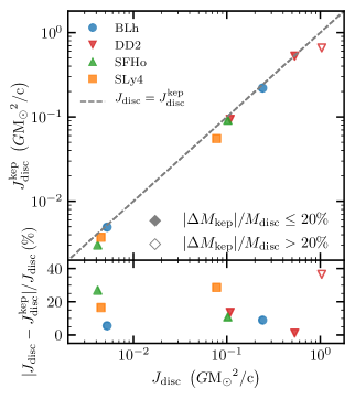
Figure 13: Top: Comparison between the disc angular momentum outside the ISCO from numerical simulations, $J_{\mathrm{d}isc}$, and the one obtained by constructing a Keplerian disc whose radial density profile was fitted over the numerical results using Eq. (12), $J_{\mathrm{d}isc}^{\mathrm{k}ep}$. Bottom: Relative difference between the two values. Unfilled markers represent discs for which the Keplerian mass differs from the numerical one by more than 20 per cent.

To better quantify this difference, in Fig. 13 we compare the angular momentum of the discs from our simulations at SR with the corresponding Keplerian analogue,Eq. (13). With the exception of DD2 EOS with $q=1.67$, the discrepancy is $<$30 per cent.

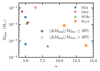
Figure 14: Power-law exponent, $\alpha$, for each disc in our numerical simulation sample, as a function of the disc mass, $M_{\mathrm{d}isc}$. Unfilled markers represent discs for which the mass inside the Keplerian disc differs from the numerical one by more than $0.2$. Massive discs have a shallower decline corresponding to smaller values of $\alpha^{\prime}s$.

In Fig. 14, we show the power-law exponent $\alpha$, obtained by fitting Eq. (13) over the numerical data as a function of $M^{\mathrm{n}um}_{\mathrm{d}isc}$. Unfilled markers represent discs for which the mass of the Keplerian disc differs from the actual one by more than $0.2$. The exponent $\alpha$ changes considerably within our sample, from 4 up to 14, and more massive discs ($M_{\mathrm{d}isc}>10^{-2}\mathrm{\,M_{\odot}}$) have a shallower decline, characterised by $4.0\lesssim\alpha\lesssim 5.4$.

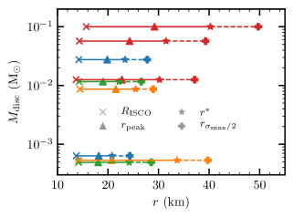
Figure 15: Fitted values of $R_{\mathrm{I}SCO}$, $r_{\mathrm{p}eak}$ and $r^{*}$ as defined in Eq. (12) for the discs reported in 13 except the simulation with error on the mass above 0.2. Solid lines represent the radius spanned by the Gaussian, while dashed lines represent the power decay branch of $\sigma(r)$ up to the radius $r_{\sigma_{\mathrm{m}ax}/2}$ at which the value of the density is half of its maximum.

The relevant parameters for the radial distributions of simulations at SR are summarised in Fig. 15. The radius of the ISCO $R_{\mathrm{I}SCO}$ (crosses), of the density peak $r_{\mathrm{p}eak}$ (up-triangles), of the junction between the Gaussian and the power decay $r^{*}$ (stars) and of the half density peak $r_{\sigma_{\mathrm{m}ax}/2}$ span a small range, indicating similar radial density distributions despite the mass spans almost 3 order of magnitude. $R_{\mathrm{I}SCO}$ is found at $13-16~{}{\mathrm{k}m}$ from the centre, while the density peak is around $17-29~{}{\mathrm{k}m}$.

Appendix B Comparison with the fitting formulae used to compute GW190425 kilonova light curves

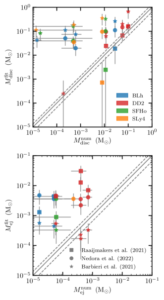
Figure 16: Top: Comparison of the disc masses obtained from our numerical simulations and from the fitting formulae used in Raaijmakers et al. (2021) (originally, from Krüger & Foucart (2020)) and in Barbieri et al. (2021). Bottom: Comparison of the dynamical ejecta masses obtained from our numerical simulations and from the fitting formulae used in Raaijmakers et al. (2021) (originally, from Krüger & Foucart (2020)) and in Barbieri et al. (2021) (originally from Radice et al. (2018b)). Fitting formulae from Nedora et al. (2022) are also reported. The error bars on the vertical (horizontal) axis are estimated as the 50 per cent of the predicted value (absolute difference between the SR and LR values). For the BNS in our sample with $M_{\mathrm{d}isk}^{\mathrm{n}um}\lesssim 10^{-3}~{}\mathrm{\,M_{\odot}}$ ($M_{\mathrm{d}isk}^{\mathrm{n}um}\lesssim 10^{-4}~{}\mathrm{\,M_{\odot}}$), the formulae from Krüger & Foucart (2020) (Nedora et al., 2022) result in nonphysical values for the disc mass.

In this appendix, we test the fitting formulae for the ejecta and disc properties used in Raaijmakers et al. (2021) and Barbieri et al. (2021) in the parameter range of GW190425 to predict the associated kilonova light curves. Some of these formulae were originally proposed in Foucart et al. (2017), Krüger & Foucart (2020), Radice et al. (2018b) (see also Dietrich & Ujevic (2017)). Additionally, we include in the comparison fitting formulae from Nedora et al. (2022) in the form of their equation 6, i.e., a second-order polynomial in the mass ratio and tidal deformability. In particular, we use coefficients fitted on the dataset RefM0Set & M0/M1Set, i.e., on a set of simulations including neutrino emission and absorption, and microphysical EOSs. We stress that we examine the different formulae in an unexplored parameter region since the binary systems within the calibration dataset are overall lighter and involve more deformable objects than those in our simulations.

In Fig. 16, we compare the disc (top) and ejecta (bottom) masses predicted by the various fitting formulae with the ones obtained by our simulations. The uncertainties in the fitted values are $50$ per cent of the estimated value, summed to a floor value of $5\times 10^{-4}\mathrm{\,M_{\odot}}$ for the disc mass and $5\times 10^{-5}\mathrm{\,M_{\odot}}$ for the ejecta mass. The bisector is the “agreement line", while the dashed lines represent the $35$ per cent deviation from the exact prediction. For the mass of the dynamical ejecta only simulations with $M_{\mathrm{e}j}>10^{-5}\mathrm{\,M_{\odot}}$ have been taken into account.

In most of the cases, the fitting formulae significantly overestimate both the mass of the disc and the mass of the dynamical ejecta, and sometimes even predict opposite trends with respect to the binary parameters. Only in the case of the disc masses predicted by Krüger & Foucart (2020) (used in Raaijmakers et al., 2021) and of the ejecta masses by Radice et al. (2018b) (used in Barbieri et al., 2021) there is a partial agreement, at least within the estimated uncertainties.

The estimates of Nedora et al. (2022) is rather insensitive to the detailed binary parameters, giving rather similar ejecta mass and disc mass for each binary configuration.

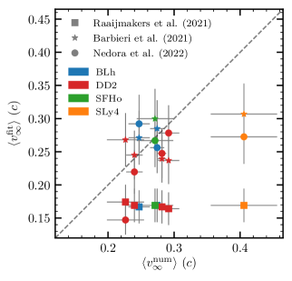
Figure 17: Comparison of the mass-weighted average velocity of the dynamical ejecta as obtained in our simulations and from the fitting formulae employed in the kilonova calculations of Raaijmakers et al. (2021) and Barbieri et al. (2021), taken from Foucart et al. (2017) and Radice et al. (2018b), respectively. Results from the fitting formulae from Nedora et al. (2022) are also reported. The (symmetric) uncertainties on the vertical axis are conservatively estimated as the 30 per cent of the values obtained from the fitting formulae. Error bars on the horizontal axis are estimated as the difference between the values inferred from the SR and LR simulations.

Another physical input needed in kilonova light curves calculations is the velocity at which ejected matter is expelled from the binary system. In Fig. 17, we show the mass-weighted average asymptotic velocity of the dynamical ejecta obtained from our numerical simulations and from the fitting formulae presented in Radice et al. (2018b); Foucart et al. (2017); Nedora et al. (2022). Only simulations with $M_{\mathrm{e}j}>10^{-5}\mathrm{\,M_{\odot}}$ have been taken into account. We assume a conservative uncertainty of the 30 per cent on the values obtained from the fitting formulae. We observe that the formulae from Radice et al. (2018b) and Nedora et al. (2022) work reasonably well for outflow speed with $\langle v_{\infty}^{\mathrm{n}um}\rangle$ in the range $0.24-0.30\,c$, while they underestimate the average velocity in the simulation with the fastest ejecta. The fitting formula from Foucart et al. (2017) used in Raaijmakers et al. (2021) to make predictions on the kilonova from the GW190425 event, but originally tailored for the dynamical ejecta of BHNS systems, predicts a very similar average velocity for all the binaries, that is systematically smaller than the outcome of the simulations. This is because the expression assumes that the average velocity of the ejecta is given by a constant value of $\sim 0.15$ plus a linear correction in the mass ratio, which is tiny in the case of BNS systems ($q\sim 1-2$).

Appendix C Standard deviation of the azimuthal angle

The azimuthal angle of the dynamical ejecta distribution $\phi_{\mathrm{e}j}$ has a $2\pi$-rotational symmetry. So its mass weighted SD $\phi_{\mathrm{e}j}^{\mathrm{S}D}$ depends on an arbitrary chosen reference. For each angular bin $\phi_{i}$ of normalised weight $w_{i}$ of the ejecta distribution we define the periodic shift $S_{\delta}(\phi_{i})$ as:

$$S_{\delta}(\phi_{i}):=\begin{cases}\phi_{i}+\delta&{\mathrm{i}f}\;\phi_{i}<2\pi-\delta~{},\\ \phi_{i}+\delta-2\pi&{\mathrm{i}f}\;\phi_{i}\geq 2\pi-\delta~{}.\\ \end{cases}$$ (25)

Let’s indicate with $S_{\delta}(\phi_{\mathrm{e}j})$ the distribution obtained after the shift of awl the $\phi_{i}$.The average $\langle\phi_{\mathrm{e}j}\rangle_{\delta}\equiv\langle S_{\delta}(\phi_{\mathrm{e}j})\rangle$ is then

$$\langle\phi_{\mathrm{e}j}\rangle_{\delta}=\langle\phi_{\mathrm{e}j}\rangle_{0}+\delta-2\pi W_{\delta}\,,$$ (26)

where $W_{\delta}$ is the total weight of the bins $\phi_{i}\geq 2\pi-\delta$,

$$W_{\delta}=\sum_{\phi_{i}\geq 2\pi-\delta}w_{i}\leq 1\,.$$ (27)

We choose $\delta=\delta^{*}$ such that $\langle\phi_{\mathrm{e}j}\rangle_{\delta}$ is centred in the half of the interval, i.e in $\pi$ :

$$\delta^{*}-2\pi W_{\delta^{*}}=\pi-\langle\phi_{\mathrm{e}j}\rangle_{0}\,.$$ (28)

The root mean square (RMS) of $\phi_{\mathrm{e}j}$ after the shift $S_{\delta}$ is

$$\begin{split}{\mathrm{R}MS}_{\delta}(\phi_{\mathrm{e}j})=\bigg{[}&{\mathrm{R}MS}_{0}(\phi_{\mathrm{e}j})^{2}+2\delta\langle\phi_{\mathrm{e}j}\rangle_{0}+\delta^{2}+\\ &+4\pi\left((\pi-\delta)W_{\delta}-\overline{\langle\phi_{\mathrm{e}j}\rangle}_{\delta}\right)\bigg{]}^{1/2}\,,\end{split}$$ (29)

where ${\mathrm{R}MS}_{0}(\phi_{\mathrm{e}j})$ and $\langle\phi_{\mathrm{e}j}\rangle_{0}$ are the unshifted RMS and average of $\phi$ and $\overline{\langle\phi_{\mathrm{e}j}\rangle}_{\delta}$ is the average of the bins $\phi_{i}\geq 2\pi-\delta$,

$$\overline{\langle\phi_{\mathrm{e}j}\rangle}_{\delta}=\sum_{\phi_{i}\geq 2\pi-\delta}w_{i}\phi_{i}\,.$$ (30)

Finally, the SD with respect to the new average $\langle\phi_{\mathrm{e}j}\rangle_{\delta}$ is

$$\begin{split}\sigma_{\delta}(\phi_{\mathrm{e}j})&=\sqrt{\sum_{i}w_{i}(S_{\delta}(\phi_{i})-\langle\phi_{\mathrm{e}j}\rangle_{\delta})^{2}}\\ &=\sqrt{{\mathrm{R}MS}_{\delta}(\phi_{\mathrm{e}j})^{2}-\langle\phi_{\mathrm{e}j}\rangle_{\delta}^{2}}\,.\end{split}$$ (31)

References

- Aasi et al. (2015) Aasi J., et al., 2015, Class. Quant. Grav., 32, 074001
- Abbott et al. (2017a) Abbott B. P., et al., 2017a, Phys. Rev. Lett., 119, 161101
- Abbott et al. (2017b) Abbott B. P., et al., 2017b, Astrophys. J., 848, L12
- Abbott et al. (2018) Abbott B. P., et al., 2018, Phys. Rev. Lett., 121, 161101
- Abbott et al. (2019a) Abbott B. P., et al., 2019a, Phys. Rev., X9, 011001
- Abbott et al. (2019b) Abbott B. P., et al., 2019b, Phys. Rev., X9, 031040
- Abbott et al. (2020) Abbott B., et al., 2020, Astrophys. J. Lett., 892, L3
- Abbott et al. (2021a) Abbott R., et al., 2021a
- Abbott et al. (2021b) Abbott R., et al., 2021b
- Abbott et al. (2021c) Abbott R., et al., 2021c, Phys. Rev. X, 11, 021053
- Acernese et al. (2015) Acernese F., et al., 2015, Class. Quant. Grav., 32, 024001
- Akmal et al. (1998) Akmal A., Pandharipande V. R., Ravenhall D. G., 1998, Phys. Rev., C58, 1804
- Akutsu et al. (2019) Akutsu T., et al., 2019, Nature Astron., 3, 35
- Andreoni et al. (2021) Andreoni I., et al., 2021
- Antier et al. (2020) Antier S., et al., 2020, Mon. Not. Roy. Astron. Soc., 497, 5518
- Aso et al. (2013) Aso Y., Michimura Y., Somiya K., Ando M., Miyakawa O., Sekiguchi T., Tatsumi D., Yamamoto H., 2013, Phys. Rev. D, 88, 043007
- Baiotti & Rezzolla (2017) Baiotti L., Rezzolla L., 2017, Rept. Prog. Phys., 80, 096901
- Barbieri et al. (2019) Barbieri C., Salafia O. S., Perego A., Colpi M., Ghirlanda G., 2019, Astron. Astrophys., 625, A152
- Barbieri et al. (2020) Barbieri C., Salafia O. S., Perego A., Colpi M., Ghirlanda G., 2020, Eur. Phys. J., A56, 8
- Barbieri et al. (2021) Barbieri C., Salafia O. S., Colpi M., Ghirlanda G., Perego A., 2021, Astron. Astrophys., 654, A12
- Barnes et al. (2016) Barnes J., Kasen D., Wu M.-R., Martinez-Pinedo G., 2016, Astrophys. J., 829, 110
- Bauswein et al. (2013) Bauswein A., Goriely S., Janka H.-T., 2013, Astrophys.J., 773, 78
- Bernuzzi (2020) Bernuzzi S., 2020, Gen. Rel. Grav., 52, 108
- Bernuzzi & Hilditch (2010) Bernuzzi S., Hilditch D., 2010, Phys. Rev., D81, 084003
- Bernuzzi et al. (2020) Bernuzzi S., et al., 2020, Mon. Not. Roy. Astron. Soc.
- Boersma et al. (2021) Boersma O., et al., 2021, Astron. Astrophys., 650, A131
- Bombaci & Logoteta (2018) Bombaci I., Logoteta D., 2018, Astron. Astrophys., 609, A128
- Bovard et al. (2017) Bovard L., Martin D., Guercilena F., Arcones A., Rezzolla L., Korobkin O., 2017, Phys. Rev., D96, 124005
- Brandt et al. (2021) Brandt S. R., et al., 2021, The Einstein Toolkit, doi:10.5281/zenodo.5770803, https://doi.org/10.5281/zenodo.5770803
- Breschi et al. (2021) Breschi M., Perego A., Bernuzzi S., Del Pozzo W., Nedora V., Radice D., Vescovi D., 2021, Mon. Not. Roy. Astron. Soc., 505, 1661
- Brügmann et al. (2008) Brügmann B., Gonzalez J. A., Hannam M., Husa S., Sperhake U., et al., 2008, Phys.Rev., D77, 024027
- Bulla (2019) Bulla M., 2019, Mon. Not. Roy. Astron. Soc., 489, 5037
- Capano et al. (2020) Capano C. D., et al., 2020, Nature Astron., 4, 625
- Coughlin et al. (2019) Coughlin M. W., et al., 2019, Astrophys. J. Lett., 885, L19
- Cromartie et al. (2019) Cromartie H. T., et al., 2019, Nat. Astron., 4, 72
- Damour (1983) Damour T., 1983, in Deruelle N., Piran T., eds, Gravitational Radiation. North-Holland, Amsterdam, pp 59–144
- Dietrich & Bernuzzi (2015) Dietrich T., Bernuzzi S., 2015, Phys.Rev., D91, 044039
- Dietrich & Ujevic (2017) Dietrich T., Ujevic M., 2017, Class. Quant. Grav., 34, 105014
- Dietrich et al. (2017) Dietrich T., Ujevic M., Tichy W., Bernuzzi S., Brügmann B., 2017, Phys. Rev., D95, 024029
- Dietrich et al. (2018) Dietrich T., et al., 2018, Class. Quant. Grav., 35, 24LT01
- Dietrich et al. (2021) Dietrich T., Hinderer T., Samajdar A., 2021, Gen. Rel. Grav., 53, 27
- Douchin & Haensel (2001) Douchin F., Haensel P., 2001, Astron. Astrophys., 380, 151
- Dudi et al. (2021) Dudi R., et al., 2021
- Eichler et al. (2015) Eichler M., et al., 2015, Astrophys. J., 808, 30
- Fahlman & Fernández (2022) Fahlman S., Fernández R., 2022, Mon. Not. Roy. Astron. Soc., 513, 2689
- Fernández et al. (2019) Fernández R., Tchekhovskoy A., Quataert E., Foucart F., Kasen D., 2019, Mon. Not. Roy. Astron. Soc., 482, 3373
- Foucart et al. (2017) Foucart F., et al., 2017, Class. Quant. Grav., 34, 044002
- Galeazzi et al. (2013) Galeazzi F., Kastaun W., Rezzolla L., Font J. A., 2013, Phys.Rev., D88, 064009
- Goodale et al. (2003) Goodale T., Allen G., Lanfermann G., Massó J., Radke T., Seidel E., Shalf J., 2003, in Vector and Parallel Processing – VECPAR’2002, 5th International Conference, Lecture Notes in Computer Science. Springer, Berlin
- Goriely (2015) Goriely S., 2015, Eur. Phys. J. A, 51, 22
- Gourgoulhon et al. (2001) Gourgoulhon E., Grandclement P., Taniguchi K., Marck J.-A., Bonazzola S., 2001, Phys.Rev., D63, 064029
- Han et al. (2020) Han M.-Z., Tang S.-P., Hu Y.-M., Li Y.-J., Jiang J.-L., Jin Z.-P., Fan Y.-Z., Wei D.-M., 2020, Astrophys. J., 891, L5
- Hempel & Schaffner-Bielich (2010) Hempel M., Schaffner-Bielich J., 2010, Nucl. Phys., A837, 210
- Hilditch et al. (2013) Hilditch D., Bernuzzi S., Thierfelder M., Cao Z., Tichy W., Bruegmann B., 2013, Phys. Rev., D88, 084057
- Hinderer (2008) Hinderer T., 2008, Astrophys.J., 677, 1216
- Hotokezaka & Nakar (2019) Hotokezaka K., Nakar E., 2019, ] 10.3847/1538-4357/ab6a98
- Hotokezaka et al. (2013) Hotokezaka K., Kiuchi K., Kyutoku K., Okawa H., Sekiguchi Y.-i., et al., 2013, Phys.Rev., D87, 024001
- Jiang et al. (2020) Jiang J.-L., Tang S.-P., Wang Y.-Z., Fan Y.-Z., Wei D.-M., 2020, Astrophys. J., 892, 1
- Just et al. (2015) Just O., Bauswein A., Pulpillo R. A., Goriely S., Janka H. T., 2015, Mon. Not. Roy. Astron. Soc., 448, 541
- Kawaguchi et al. (2016) Kawaguchi K., Kyutoku K., Shibata M., Tanaka M., 2016, Astrophys. J., 825, 52
- Kawaguchi et al. (2018) Kawaguchi K., Shibata M., Tanaka M., 2018, Astrophys. J., 865, L21
- Kawaguchi et al. (2020) Kawaguchi K., Shibata M., Tanaka M., 2020, Astrophys. J., 889, 171
- Korobkin et al. (2012) Korobkin O., Rosswog S., Arcones A., Winteler C., 2012, Mon. Not. Roy. Astron. Soc., 426, 1940
- Krüger & Foucart (2020) Krüger C. J., Foucart F., 2020, Phys. Rev. D, 101, 103002
- Kyutoku et al. (2014) Kyutoku K., Shibata M., Taniguchi K., 2014, Phys. Rev., D90, 064006
- Kyutoku et al. (2020) Kyutoku K., Fujibayashi S., Hayashi K., Kawaguchi K., Kiuchi K., Shibata M., Tanaka M., 2020, Astrophys. J., 890, L4
- Lehner et al. (2016) Lehner L., Liebling S. L., Palenzuela C., Caballero O. L., O’Connor E., Anderson M., Neilsen D., 2016, Class. Quant. Grav., 33, 184002
- Lippuner & Roberts (2015) Lippuner J., Roberts L. F., 2015, Astrophys. J., 815, 82
- Lippuner & Roberts (2017) Lippuner J., Roberts L. F., 2017, Astrophys. J. Suppl., 233, 18
- Lippuner et al. (2017) Lippuner J., Fernández R., Roberts L. F., Foucart F., Kasen D., Metzger B. D., Ott C. D., 2017, Mon. Not. Roy. Astron. Soc., 472, 904
- Loffler et al. (2012) Loffler F., et al., 2012, Class. Quant. Grav., 29, 115001
- Logoteta et al. (2021) Logoteta D., Perego A., Bombaci I., 2021, Astron. Astrophys., 646, A55
- Margutti & Chornock (2021) Margutti R., Chornock R., 2021, Ann. Rev. Astron. Astrophys., 59, 155
- Martin et al. (2018) Martin D., Perego A., Kastaun W., Arcones A., 2018, Class. Quant. Grav., 35, 034001
- Miller et al. (2019) Miller M. C., et al., 2019, Astrophys. J., 887, L24
- Most et al. (2021) Most E. R., Papenfort L. J., Tootle S., Rezzolla L., 2021, Astrophys. J., 912, 80
- Nedora et al. (2021a) Nedora V., Radice D., Bernuzzi S., Perego A., Daszuta B., Endrizzi A., Prakash A., Schianchi F., 2021a, preprint (ArXiv:2104.04537)
- Nedora et al. (2021b) Nedora V., et al., 2021b, Astrophys. J., 906, 98
- Nedora et al. (2022) Nedora V., et al., 2022, Class. Quant. Grav., 39, 015008
- Neilsen et al. (2014) Neilsen D., Liebling S. L., Anderson M., Lehner L., O’Connor E., et al., 2014, Phys.Rev., D89, 104029
- Perego et al. (2017) Perego A., Radice D., Bernuzzi S., 2017, Astrophys. J., 850, L37
- Perego et al. (2022) Perego A., et al., 2022, Astrophys. J., 925, 22
- Pinto & Eastman (2000) Pinto P. A., Eastman R. G., 2000, Astrophys. J., 530, 744
- Pollney et al. (2011) Pollney D., Reisswig C., Schnetter E., Dorband N., Diener P., 2011, Phys. Rev., D83, 044045
- Prantzos et al. (2020) Prantzos N., Abia C., Cristallo S., Limongi M., Chieffi A., 2020, mnras, 491, 1832
- Raaijmakers et al. (2021) Raaijmakers G., et al., 2021, Astrophys. J., 922, 269
- Radice (2020) Radice D., 2020, Symmetry, 12, 1249
- Radice & Rezzolla (2012) Radice D., Rezzolla L., 2012, Astron. Astrophys., 547, A26
- Radice et al. (2014) Radice D., Rezzolla L., Galeazzi F., 2014, Mon.Not.Roy.Astron.Soc., 437, L46
- Radice et al. (2016) Radice D., Galeazzi F., Lippuner J., Roberts L. F., Ott C. D., Rezzolla L., 2016, Mon. Not. Roy. Astron. Soc., 460, 3255
- Radice et al. (2018a) Radice D., Perego A., Bernuzzi S., Zhang B., 2018a, Mon. Not. Roy. Astron. Soc., 481, 3670
- Radice et al. (2018b) Radice D., Perego A., Hotokezaka K., Fromm S. A., Bernuzzi S., Roberts L. F., 2018b, Astrophys. J., 869, 130
- Radice et al. (2020) Radice D., Bernuzzi S., Perego A., 2020, Ann. Rev. Nucl. Part. Sci., 70
- Read et al. (2009) Read J. S., Lackey B. D., Owen B. J., Friedman J. L., 2009, Phys. Rev., D79, 124032
- Reisswig et al. (2013a) Reisswig C., Ott C., Abdikamalov E., Haas R., Mösta P., et al., 2013a, Phys.Rev.Lett., 111, 151101
- Reisswig et al. (2013b) Reisswig C., Haas R., Ott C. D., Abdikamalov E., Mösta P., Pollney D., Schnetter E., 2013b, Phys. Rev., D87, 064023
- Riley et al. (2019) Riley T. E., et al., 2019, Astrophys. J., 887, L21
- Rosswog (2015) Rosswog S., 2015, Int.J.Mod.Phys., D24, 1530012
- Ruffert et al. (1996) Ruffert M. H., Janka H. T., Schäfer G., 1996, Astron. Astrophys., 311, 532
- Schneider et al. (2017) Schneider A. S., Roberts L. F., Ott C. D., 2017, Phys. Rev., C96, 065802
- Schnetter et al. (2004) Schnetter E., Hawley S. H., Hawke I., 2004, Class.Quant.Grav., 21, 1465
- Schnetter et al. (2007) Schnetter E., Ott C. D., Allen G., Diener P., Goodale T., Radke T., Seidel E., Shalf J., 2007
- Sekiguchi et al. (2015) Sekiguchi Y., Kiuchi K., Kyutoku K., Shibata M., 2015, Phys.Rev., D91, 064059
- Shibata & Hotokezaka (2019) Shibata M., Hotokezaka K., 2019, Ann. Rev. Nucl. Part. Sci., 69, 41
- Shibata et al. (2017) Shibata M., Fujibayashi S., Hotokezaka K., Kiuchi K., Kyutoku K., Sekiguchi Y., Tanaka M., 2017, Phys. Rev., D96, 123012
- Siegel & Metzger (2017) Siegel D. M., Metzger B. D., 2017, Phys. Rev. Lett., 119, 231102
- Steeghs et al. (2019) Steeghs D., et al., 2019, GRB Coordinates Network, 24224, 1
- Steiner et al. (2013) Steiner A. W., Hempel M., Fischer T., 2013, Astrophys. J., 774, 17
- Tanaka et al. (2020) Tanaka M., Kato D., Gaigalas G., Kawaguchi K., 2020, Mon. Not. Roy. Astron. Soc., 496, 1369
- Thierfelder et al. (2011) Thierfelder M., Bernuzzi S., Hilditch D., Brügmann B., Rezzolla L., 2011, Phys.Rev., D83, 064022
- Thornburg (2004) Thornburg J., 2004, Class. Quant. Grav., 21, 743
- Typel et al. (2010) Typel S., Ropke G., Klahn T., Blaschke D., Wolter H. H., 2010, Phys. Rev., C81, 015803
- Wanajo et al. (2014) Wanajo S., Sekiguchi Y., Nishimura N., Kiuchi K., Kyutoku K., Shibata M., 2014, Astrophys. J., 789, L39
- Wollaeger et al. (2018) Wollaeger R. T., et al., 2018, Mon. Not. Roy. Astron. Soc., 478, 3298
- Wu et al. (2016) Wu M.-R., Fernández R., Martínez-Pinedo G., Metzger B. D., 2016, Mon. Not. Roy. Astron. Soc., 463, 2323
- Wu et al. (2021) Wu Z., Ricigliano G., Kashyap R., Perego A., Radice D., 2021
- Zappa et al. (2018) Zappa F., Bernuzzi S., Radice D., Perego A., Dietrich T., 2018, Phys. Rev. Lett., 120, 111101
- de Jesús Mendoza-Temis et al. (2015) de Jesús Mendoza-Temis J., Wu M.-R., Martinez-Pinedo G., Langanke K., Bauswein A., Janka H.-T., 2015, Phys. Rev., C92, 055805
- Özel & Freire (2016) Özel F., Freire P., 2016, Ann. Rev. Astron. Astrophys., 54, 401