A Multipolar Effective One Body Model for Non-Spinning Black Hole Binaries

Abstract

We introduce TEOBiResumMultipoles, a nonspinning inspiral-merger-ringdown waveform model built within the effective one body (EOB) framework that includes gravitational waveform modes beyond the dominant quadrupole $(\ell,|m|)=(2,2)$. The model incorporates: (i) an improved Padé resummation of the factorized waveform amplitudes $\rho_{\ell m}^{\rm orb}$ entering the EOB-resummed waveform where the 3PN, mass-ratio dependent, terms are hybridized with test-mass limit terms up to 6PN relative order for most of the multipoles up to $\ell=6$ included; (ii) an improved determination of the effective 5PN function $a_{6}^{c}(\nu)$ entering the EOB interaction potential done using the most recent, error-controlled, nonspinning numerical relativity (NR) waveforms from the Simulating eXtreme Spacetimes (SXS) collaboration; and (iii) a NR-informed phenomenological description of the multipolar ringdown. Such representation stems from 19 NR waveforms with mass ratios up to $m_{1}/m_{2}=18$ as well as test-mass waveform data, although it does not incorporate mode-mixing effects. The NR-completed higher modes through merger and ringdown considered here are: $(\ell,|m|)=\{(2,1),(3,3),(3,2),(3,1),(4,4),(4,3),(4,2),(4,1),(5,5)\}$. For simplicity, the other subdominant modes, up to $\ell=8$, are approximated by the corresponding, purely analytical, factorized and resummed EOB waveform. To attempt an estimate of (some of) the underlying analytic uncertainties of the model, we also contrast the effect of the 6PN-hybrid Padé-resummed $\rho_{\ell m}$’s with the standard $3^{+2}$ PN, Taylor-expanded, ones used in previous EOB works. The maximum unfaithfulness $\bar{F}$ against the SXS waveforms including all NR-completed modes up to $\ell=m=5$ is always $\lesssim 2$% for binaries with total mass $M$ as $50M_{\odot}\leq M\lesssim 200M_{\odot}$. The Padé-resummed multipolar EOB model for nonspinning binaries discussed here defines the foundations of a multipolar EOB waveform model for spin-aligned binaries that will be introduced in a companion paper.

I Introduction

The recent observation made by LIGO Aasi et al. (2015) and Virgo Acernese et al. (2015) of gravitational wave signals (GWs) from eleven coalescing compact binaries marked the beginning of the era of gravitational wave astronomy. Of these detections, ten have been associated to binary black holes (BBH) Abbott et al. (2016a, b, 2017a, 2017b, 2017c, 2018a) as well as the detection of a coalescing binary neutron star (BNS) Abbott et al. (2017d).

One of the standard tools in modelled GW data analysis is matched filtering, implicitly demanding high-fidelity, low-bias waveform models. Search pipelines can detect GW signals from binary black holes by cross-correlation of the data against theoretical waveform templates for the expected signal. Bayesian parameter estimation allows us to infer the source properties of the binary by comparing the data against our analytical waveform families. Null tests of General Relativity (GR) are often predicated on the comparison of the data to the faithful representations of GR given by our waveform models. It is therefore vital that our waveform models are accurate and incorporate as much physics as possible. A deficiency in many waveform families to date has been that they only model the leading quadrupole $(\ell=2,m=2)$ mode of gravitational radiation. For weak signal to noise ratio (SNR) observations or for binaries where intrinsic asymmetries are suppressed, i.e. comparable mass ratios and near equal spin configurations, this may be sufficient. This simplification was sufficiently accurate for detecting the binary black hole sources observed during the first two LIGO - Virgo observing runs (O1 and O2), with no compelling evidence for higher modes seen in the parameter estimation  Abbott et al. (2017e, 2018a).

However, with the sensitivity of Advanced LIGO and Virgo ever increasing, systematic errors will start to dominate statistical errors leading to potentially large biases in our parameter estimation O’Shaughnessy et al. (2014); Varma and Ajith (2017) and could degrade the performance of our search pipelines Capano et al. (2014); Calderón Bustillo et al. (2017); Harry et al. (2018). Specifically, this could be the case for binaries that have high inclination angles or where there are stronger intrinsic asymmetries, such as one BH being more massive than the other or large unequal spin effects. Similarly, at large inclinations, the modeling of gravitational wave modes beyond the dominant mode becomes increasingly important as higher modes are geometrically suppressed in the face-on/off limit.

A key result in GR is the no-hair theorem, in which the quasi-normal-modes (QNMs) of an isolated BH in GR may only depend on the BH’s mass $M_{\rm BH}$, angular momentum $J_{\rm BH}$ or charge $Q$. In vacuum, testing the no-hair theorem requires us to identify at least two QNMs in the ringdown, necessitating accurate higher-mode waveforms for binary black holes. Recent studies on such black hole spectroscopy have demonstrated the feasibility of performing such tests of general relativity Dreyer et al. (2004); Berti et al. (2006); Kamaretsos et al. (2012a); Gossan et al. (2012); Kamaretsos et al. (2012b); Meidam et al. (2014); London et al. (2014); Berti et al. (2016); Cardoso and Gualtieri (2016); Yang et al. (2017); Brito et al. (2018); Carullo et al. (2018).

Within the effective-one-body (EOB) approach, the first model including higher-order modes in the nonspinning case was presented in Ref. Pan et al. (2011), now known as EOBNRv2HM, followed by Ref. Damour et al. (2013), that employed different EOB dynamics. More recently Ref. Cotesta et al. (2018) improved the EOBNRv2HM model, generalizing it to the case of spin-aligned BBHs. This model is called SEOBNRv4HM and it is currently the only available EOB model with higher harmonics. In the IMRPhenom family of waveform models, Mehta et al. (2017) presented a non-spinning model calibrated against NR and London et al. (2018) used approximate analytical relations to construct an uncalibrated higher mode model for spin-aligned BBHs.

In this paper we follow up on the work of Ref. Damour et al. (2013). To do so, we improve the nonspinning sector of TEOBResumS Nagar et al. (2018) by completing the EOB-resummed multipolar waveform through merger and ringdown with all subdominant multipoles up to $\ell=m=5$ included. This result crucially relies on an improved representation of the merger-ringdown waveform that builds upon the post-merger analytical description of Refs. Damour and Nagar (2014a); Del Pozzo and Nagar (2017) that is informed by suitable fits of a few ($19$) Numerical Relativity (NR) nonspinning waveforms. Comparable-mass NR data are also complemented by the test-mass waveform data of Harms et al. (2014). Our important conceptual finding is that, once that the NR information is represented analytically, the procedure to match the post-merger waveform to the inspiral EOB waveform is precisely the same for all multipoles, without any special ad-hoc tuning and/or calibration for each mode. Moreover, we also improve the dynamical sector of the model, by augmenting the multipolar waveform amplitudes with test-particle information and/or Padé resumming them. This in turn needs a new determination of the effective coefficient $a_{6}^{c}$ that enters the EOB interaction potential at 5th post-Newtonian (PN) order and is informed by NR simulations. The nonspinning dynamics presented here will then be used for the generalization of the multipolar waveform model to the spin-aligned case, that will be presented in a separate publication.

A complementary approach was presented in Borhanian et al. (2019), which studies the structure of the multipolar waveform throughout the transition from the perturbative inspiral regime to the highly non-perturbative merger using a combination of post-Newtonian theory and numerical relativity data. There it is shown that the dependencies of the dominant modes amplitudes on the symmetric mass ratio and binary spin, to leading order in post-Newtonian theory, agree remarkably well with those from numerical relativity even in a regime in which this approximation should have broken down.

This paper is organized as follows: In Sec. II we recall the phenomenology due to the presence of higher waveform modes. Section III discusses in detail all the building blocks of the nonspinning EOB model, with special emphasis on the analytical structure of the waveform multipoles; Section IV focuses on how the EOB dynamics is informed by NR simulations through the determination of $a_{6}^{c}$, highlighting the differences with respect to previous work; Section V illustrates in high detail the construction of the merger and postmerger multipolar waveform model, reporting all the NR-informed fits needed, while the phasing accuracy of the model is assessed in Sec. VII, either via standard time-domain phasing comparisons or via unfaithfulnesses analyses. Our concluding remarks are reported in Sec. VIII. Unless stated otherwise, we use geometrized units with $G=c=1$ and the following notation: $M\equiv m_{1}+m_{2}$, $\mu\equiv m_{1}m_{2}/M$, $\nu\equiv\mu/M$ with the convention that the mass ratio is $q\equiv m_{1}/m_{2}\geq 1$.

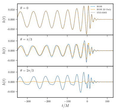
Figure 1: Illustrating the effect of higher multipoles. Comparison of $h(t)$ between the EOB model and SXS:0303, a non-spinning binary of mass ratio $q=10$.

II Waveform phenomenology due to higher-order modes

The time-domain complex gravitational wave strain can be written in terms of the spin weighted spherical harmonics as

$$h_{+}(\theta,\varphi;t)-{\rm i}h_{\times}(\theta,\varphi;t)$$

$$\qquad\quad=\dfrac{GM}{{\cal D}_{L}c^{2}}\displaystyle\sum_{\ell=2}^{\infty}\displaystyle\sum_{m=-\ell}^{\ell}\,\,h_{\ell m}(t)_{-2}Y_{\ell m}(\theta,\varphi)\ ,$$ (1)

where $\{\theta,\varphi\}$ are the spherical angles in a coordinate system with the z-axis aligned along the orbital angular momentum and ${D_{L}}$ the luminosity distance from the source. The spherical harmonic modes $h_{\ell m}(t)$ are functions of the intrinsic parameters of the system with the angular dependence of the emitted gravitational radiation being governed by the spin weighted spherical harmonic basis functions. The gravitational wave strain measured by a detector will therefore be highly dependent on the sky location and inclination of the binary with respect to the observer, as the spherical harmonics effectively act as a geometric factor contributing to the relative strength of the higher modes. For face-on/face-off binaries ($\theta\sim 0$), the dominant contribution to the signal is from the quadrupolar ($\ell=2$, $m=\pm 2$) mode, as shown in the top panel of Figure 1. However, for more generic orientations, the higher modes can be of a comparable order of magnitude to the $(2,2)$ mode with the relative contribution of the higher modes depending on the underlying symmetries of the binary. This can be seen in the bottom two panels of Fig. 1. We can cleary see that the pure quadrupolar waveforms fails to capture the morphology of the signal for generic orientations. An additional simplification can be made for non-precessing binaries as there will also be a reflection symmetry about the orbital plane such that $h_{\ell m}=(-1)^{\ell}\,h_{\ell-m}^{\ast}$. This means that we can restrict our discussion to modes with $m>0$ and can use the above relation in order to reconstruct the negative $m$ modes.

III Nonspinning effective one body model

The dynamics of the multipolar EOB model we discuss here stems from a slightly modified version of the nonspinning sector of TEOBResumS Nagar et al. (2018). The analytical modifications mainly regard the radiation reaction sector, where we incorporate more analytical information than previously used in Nagar et al. (2018). In addition, due to the availability of NR waveforms from the SXS collaboration with a smaller overall error budget, it was possible to improve the model by re-informing the effective 5PN parameter $a_{6}^{c}$. For self-consistency, we detail all the various building blocks of the model, highlighting the core changes with respect to Nagar et al. (2018).

III.1 Hamiltonian

The conservative dynamics of two bodies of masses $m_{1}$ and $m_{2}$ is described by a Hamiltonian $H_{\rm{EOB}}(Q^{i},P_{i})$ in terms of the relative motion of the binary, where $R=|Q^{i}|$ is the binary separation in EOB coordinates. The Hamiltonian will depend on two radial functions $A(R)$ and $B(R)$, where $A(R)$ is the EOB radial potential. In the above notation, the EOB Hamiltonian is given by

$$\hat{H}_{\rm{EOB}}\equiv\frac{H_{\rm{EOB}}}{\mu}=\frac{1}{\nu}\sqrt{1+2\nu\left(\hat{H}_{\rm{eff}}-1\right)},$$ (2)

where the usual effective EOB Hamiltonian is

$$\hat{H}_{\rm{eff}} =\sqrt{p^{2}_{r_{\ast}}+A(r,\nu)\left(1+\frac{p_{\varphi}^{2}}{r^{2}}+\mathcal{Q}_{4}\right)},$$ (3)

with $\mathcal{Q}_{4}=2\nu(4-3\nu)p^{4}_{r_{\ast}}$ taken at 3PN accuracy Damour et al. (2000). Here, $\{r,p_{r_{\ast}},\varphi,p_{\varphi}\}$ are the usual dimensionless EOB phase space variables in polar coordinates Damour and Nagar (2014b) and we have replaced the conjugate momentum $p_{r}$ by the tortoise rescaled variable $p_{r_{\ast}}=(A/B)^{1/2}\,p_{r}$, where $r_{\ast}=\int dr(A/B)^{1/2}$. We restrict our attention to orbits confined to the equatorial plane, $\theta=\pi/2$. The dimensionless EOB phase space variables are related to the dimensionful variables $(R,P_{R},\varphi,P_{\varphi})$ by

$$r=\frac{R}{GM},\;p_{r_{\ast}}=\frac{P_{R_{\ast}}}{\mu},\;p_{\varphi}=\frac{P_{\varphi}}{\mu GM},\;t=\frac{T}{GM}.$$ (4)

Hamilton’s equations naturally follow from the above expressions and can be explicitly written as

$$\frac{d\varphi}{dt} =\Omega=\frac{\partial\hat{H}_{\rm EOB}}{\partial p_{\varphi}},$$ (5)

$$\frac{dr}{dt} =\left(\frac{A}{B}\right)^{1/2}\,\frac{\partial\hat{H}_{\rm EOB}}{\partial p_{r_{\ast}}},$$ (6)

$$\frac{dp_{\varphi}}{dt} =\hat{\mathcal{F}}_{\varphi},$$ (7)

$$\frac{dp_{r_{\ast}}}{dt} =-\left(\frac{A}{B}\right)^{1/2}\frac{\partial\hat{H}_{\rm EOB}}{\partial r}.$$ (8)

where $\hat{\mathcal{F}}_{\varphi}=\mathcal{F}_{\varphi}/\mu$ is a radiation reaction term and $\mathcal{F}_{r_{\ast}}$ is explicitly put to zero. It incorporates all multipoles, up to $\ell=8$, in special resummed form Damour et al. (2009) as detailed in Sec. III.2 below. Note that although the effect of gravitational wave absorption through the black hole horizons is small in the non-spinning case Bernuzzi et al. (2012), it is explicitly included in the model following Refs. Nagar and Akcay (2012); Bernuzzi et al. (2012).

The EOB radial potential $A(r)$ is taken with the full 4PN-accurate analytical information augmented by the 5PN logarithmic term Damour (2010); Blanchet et al. (2010); Barausse et al. (2012); Bini and Damour (2013); Damour and Nagar (2014a), as

$$A^{\rm{PN}}_{\rm{orb}}(u)=1-2u+2\nu u^{3}+\nu a_{4}u^{4}+\nu\bigg{[}a^{c}_{5}(\nu)\\ +a^{\rm{log}}_{5}\ln u\bigg{]}u^{5}+\nu\bigg{[}a^{c}_{6}(\nu)+a^{\rm{log}}_{6}\ln u\bigg{]}u^{6},$$ (9)

where $u\equiv 1/r$. The 4PN and 5PN logarithmic coefficients read

$$a^{\log}_{5} =\frac{64}{5},$$ (10)

$$a^{\log}_{6}(\nu) =-\frac{7004}{105}-\frac{144}{5}\nu,$$ (11)

while the 4PN coefficient, $a^{c}_{5}(\nu)$, is Bini and Damour (2013):

$$a^{c}_{5}(\nu) =a^{c0}_{5}+\nu a^{c1}_{5},$$ (12)

$$a^{c0}_{5} =-\frac{4237}{60}+\frac{2275}{512}\pi^{2}+\frac{256}{5}\ln 2+\frac{128}{5}\gamma_{E},$$ (13)

$$a^{c1}_{5} =-\frac{221}{6}+\frac{41}{32}\pi^{2},$$ (14)

where $\gamma_{E}$ is the Euler constant. The 5PN coefficient $a_{6}^{c}(\nu)$ is analytically known just at linear order in $\nu$ Barausse et al. (2012); the other coefficient $a_{6}^{c}(\nu)$ is here seen as an effective PN parameter that is determined, as usual, by phasing comparison with NR simulations. Before doing so, the PN-expanded radial potential $A(u)$ is Padé resummed as

$$A(u;\nu;a^{c}_{6}) =P^{1}_{5}\left[A^{\rm{PN}}_{\rm{orb}}(u)\right],$$ (15)

The other potential entering the Hamiltonian, $B(r)$, is instead taken at 3PN accuracy and is incorporated, as usual, by means of the function $D\equiv A\,B$ that is resummed by its $P^{0}_{3}$ version that reads

$$D(u) =\frac{1}{1+6\nu u^{2}+2(26-3\nu)\nu u^{3}}.$$ (16)

III.2 Resummed waveform and radiation reaction:
two different multipolar EOB models

The structure of the EOB waveform in the nonspinning case is nowadays standard Damour et al. (2009). The strain multipoles $h_{\ell m}$ are written in factorized and resummed form as

$$h_{{\ell m}}=h_{{\ell m}}^{(N,\epsilon)}\hat{S}^{(\epsilon)}_{\rm eff}\hat{h}_{{\ell m}}^{\rm tail}(y)\left[\rho^{\rm orb}_{\ell m}(x)\right]^{\ell}\hat{h}_{\ell m}^{\rm NQC},$$ (17)

where $\epsilon=(0,1)$ denotes the parity of $\ell+m$, $\hat{h}_{\ell m}^{(N,\epsilon)}$ is the Newtonian (or leading-order) contribution to each mode, $\hat{S}_{\rm eff}^{(\epsilon)}$ the effective source of the field, $\hat{h}_{\ell m}^{\rm tail}(y)$ the tail factor Damour and Nagar (2007); Damour et al. (2009), $\rho^{\rm orb}_{\ell m}$ the residual amplitude corrections and $\hat{h}_{\ell m}^{\rm NQC}$ the next-to-quasi-circular (NQC) correction factor, that will be discussed in Sec. III.4 below. The superscript “orb” stands for orbital and we explicitly write it here to ensure that our notation is consistent with that used in other work. The tail factor is written as

$$\hat{h}_{\ell m}^{\rm tail}(y)\equiv T_{\ell m}(y)e^{\rm i\delta_{\ell m}(y)},$$ (18)

where $y\equiv v_{\Omega}^{2}\equiv\Omega^{2/3}$ and the $\delta_{\ell m}(y)$ are the residual phase corrections that incorporate several test-particle limit terms and are resummed using Padé approximants following Ref. Damour et al. (2013).

The general form of the Newtonian prefactor of the circularized waveform is

$$h_{\ell m}^{(N,\epsilon)}=\nu c_{\l+\epsilon}(\nu)n_{\ell m}^{(\epsilon)}x^{(\ell+\epsilon)/2}Y^{(\ell-\epsilon,-m)}(\pi/2,\varphi),$$ (19)

where $Y(\pi/2,\varphi)$ are the scalar spherical harmonics, $n_{\ell m}^{(\epsilon)}$ are parity-dependent constants given in Eqs. (5)-(6) of Ref. Damour et al. (2009), while $c_{\l+\epsilon}(\nu)$ encode the leading-order $\nu$ dependence. For circularized binaries, $x\equiv v_{\Omega}^{2}$ is the frequency parameter. However, as pointed out long ago Damour and Gopakumar (2006); Damour and Nagar (2007), the $\ell=m=2$ waveform amplitude during the plunge is better represented by relaxing the Newtonian Kepler’s constraint and using $x=v_{\varphi}^{2}\equiv(r_{\omega}\Omega)^{2}$ with $r_{\omega}\equiv r\psi^{1/3}$, where $\psi$ is a suitably defined function such that $v_{\varphi}$ and $r_{\omega}$ satisfy Kepler’s law $1=\Omega^{2}r_{\omega}^{3}$ during the adiabatic inspiral. In the remainder of this section, we shall assume that the circular variable $x$ is always replaced by $v_{\varphi}^{2}$, since this is used in our EOB implementation of the radiation reaction. We shall however introduce exceptions to this rule when discussing the Newtonian multipolar prefactors in Sec. III.3 below.

The $\rho_{\ell m}^{\rm orb}$ functions implemented in v1.0 of TEOBResumS Nagar et al. (2018, 2019); Akcay et al. (2019) are taken following the original prescription of Refs. Damour et al. (2009); Damour and Nagar (2009), i.e. as truncated PN series at $3^{+2}$ PN order of the form $\rho_{\ell m}=1+c_{1}^{\ell m}x+c_{2}^{\ell m}x^{2}+\dots$. Here, $3^{+2}$ PN accuracy denotes that the 3PN-accurate, full $\nu$-dependent, waveform information has been augmented by test-mass terms such that the PN-order of the PN-expanded (nonresummed) flux is globally 5PN. In practice, this means that $\rho_{22}(x)$ is given by a fifth-order polynomial in $x$, i.e. $\rho_{22}(x)=1+c_{1}^{22}(\nu)x+c_{2}^{22}(\nu)x^{2}+c_{3}^{22}(\nu)x^{3}+c_{4}^{22}x^{4}+c_{5}^{22}x^{5}$, where we have explicitly highlighted the $\nu$ dependent terms, while the subdominant $\rho_{\ell m}$’s are polynomials of progressively lower order so as to be compatible with global 5PN accuracy, once multiplied by the corresponding Newtonian prefactors. In recent years, the analytical knowledge of the test-particle waveform and fluxes has been pushed to much higher PN orders Fujita (2015), notably up to 22PN in the nonspinning case Fujita (2012). It is therefore meaningful to revise and possibly improve the current choices implemented in TEOBResumS. This was explored by means of a new factorization and resummation paradigm applied to spinning waveform amplitudes introduced in Nagar and Shah (2016) and recently improved in Messina et al. (2018). The basic idea behind this approach is to (i) factorize the orbital (nonspinning) part from the spin-dependent one, so that each $\rho_{\ell m}(x)$ function is written as the product $\rho_{{\ell m}}\equiv\rho_{\ell m}^{\rm orb}\hat{\rho}_{\ell m}^{\rm S}$, where each function is of the form $1+\dots$, and (ii) to properly resum each factor. For example, in Ref. Messina et al. (2018) it was proposed to use Padé approximants for the orbital factor $\rho_{{\ell m}}^{\rm orb}$, while $\hat{\rho}^{S}_{\ell m}$ was replaced by its inverse-Taylor representation, as suggested in Nagar and Shah (2016). In particular, focusing on the test-mass limit, Ref. Messina et al. (2018) pointed out that keeping each $\rho_{\ell m}$ at 6PN order (i.e. as sixth-order polynomials) yields, after the resummation strategy described above, an excellent agreement between the analytical, resummed, residual amplitudes and the exact ones up to the light-ring, even for a quasi-extremal Kerr black hole. As a consequence, we here discuss two different treatments of the orbital $\rho_{\ell m}^{\rm orb}(x)$ that will yield two separate EOB models.

• Fully resummed waveform model. In this case, we follow the recipe of Ref. Messina et al. (2018) by first hybridizing the 3PN, $\nu$-dependent, terms in the $\rho_{\ell m}$’s with test-particle terms so that the functions are globally 6PN accurate. Then, each hybridized $\rho_{\ell m}$ is Padé resummed according to the choices of approximants listed in Table I of Messina et al. (2018). This allows us to construct an EOB model whose multipolar waveform amplitudes, and thus also the radiation reaction, are consistent with the choice of the resummed amplitudes in the large-mass ratio limit. Essentially the same choices will also be retained in the spinning case, though the factorization paradigm is applied to only the $m=\text{odd}$ multipoles up to $\ell=5$. Keeping then the nomenclature of Nagar and Shah (2016); Messina et al. (2018) for consistency, we shall address this waveform model as TEOBiResumSMultipoles, where the i prefix refers to the fact that, whenever applied, the spin-dependent factors in the waveform are resummed by taking their inverse Taylor expansions.

• Improved Taylor-expanded waveform model. In this implementation, we use the usual Taylor-expanded expression of the $\rho_{\ell m}^{\rm orb}$ at $3^{+}2$ PN order, with the only exception being $\rho_{44}^{\rm orb}$, which also incorporates the (relative) 5PN test-particle coefficient. More precisely, this function reads

  $$\rho_{44}^{\rm orb}(x) =1+c_{1}^{44}(\nu)x+c_{2}^{\rm 44}(\nu)x^{2}$$ (20)

  $$+c^{44}_{3}x^{3}+c^{44}_{4}x^{4}+c^{44}_{5}x^{5},$$

  where the coefficient

  $$c_{5}^{44} \equiv-\dfrac{17154485653213713419357}{568432724020761600000}$$

  $$+\dfrac{22324502267}{3815311500}{\rm eulerlog}_{4}(x)$$ (21)

  is omitted in the current version of the TEOBResumS model. We have, however, verified that including this term is useful to improve the agreement between the $(4,4)$ analytical and numerical waveform amplitudes up to merger. In addition to this, another key difference with respect to TEOBResumS relates to the approximation of the second time derivative of the radial separation (which enters the NQC factors) and a more demanding determination (with respect to NR uncertainties) of the effective 5PN parameters $a_{6}^{c}$. Though these choices will not be ported to the spinning case, they allow us to define a self-consistent, multipolar, EOB model for non-spinning binaries that we denote EOBResumMultipoles⁺.

The differences in the analytical representation of the $\rho_{\ell m}^{\rm orb}$’s reflect in two different determinations of the function $a_{6}^{c}(\nu)$ by NR/EOB phasing comparisons. We shall address this issue in Sec. IV below, by relying on SXS waveforms with reduced phase uncertainty that were not available at the time of Ref. Nagar et al. (2016).

III.3 Newtonian prefactors in the waveform

As mentioned above, the standard procedure to improve the behavior of the Newtonian prefactor of the circularized waveform during the plunge is to replace $x\to v_{\varphi}^{2}$ multipole by multipole. However, such simple choice makes the amplitude of some multipoles too small towards merger with respect to the corresponding NR one. This in turn makes the standard NQC factor (that will be detailed below) unable to correctly modify the bare EOB multipole. In fact, one experimentally finds that the NQC amplitude correction factor is particularly efficient when the peak of the purely analytical EOB waveform amplitude is larger than the NR one. To implement this condition efficiently, we then act as follows. Instead of completely replacing $v_{\Omega}$ with $v_{\varphi}$, we just replace some of the powers entering the Newtonian prefactor, with a choice that depends on the multipole. The aim of such pragmatic choice is essentially to mimic the effect of the missing noncircular terms in the specific multipole, and help the action of the NR-informed NQC factor. In practice we found that the following choices best recover NR amplitudes:

$$h_{22}^{(N,0)} =-8\sqrt{\dfrac{\pi}{5}}\nu\,v_{\varphi}^{2}e^{-2{\rm i}\varphi},$$ (22)

$$h_{21}^{(N,1)} =-\dfrac{8{\rm i}}{3}\sqrt{\dfrac{\pi}{5}}\nu\sqrt{1-4\nu}\,v_{\varphi}^{3}e^{-{\rm i}\varphi},$$ (23)

$$h_{33}^{(N,0)} =3{\rm i}\sqrt{\dfrac{6\pi}{7}}\nu\sqrt{1-4\nu}\,v_{\varphi}v_{\Omega}^{2}e^{-3{\rm i}\varphi},$$ (24)

$$h_{32}^{(N,1)} =\dfrac{8}{3}\sqrt{\dfrac{\pi}{7}}\nu(1-3\nu)\,v_{\varphi}^{2}v_{\Omega}^{2}e^{-2{\rm i}\varphi},$$ (25)

$$h_{31}^{(N,0)} =-\dfrac{{\rm i}}{3}\sqrt{\dfrac{2\pi}{35}}\nu\sqrt{1-4\nu}v_{\Omega}^{3}e^{-{\rm i}\varphi},$$ (26)

$$h_{44}^{(N,0)} =-\dfrac{64}{9}\sqrt{\dfrac{\pi}{7}}\nu(1-3\nu)\,v_{\varphi}^{2}v_{\Omega}^{2}e^{-4{\rm i}\varphi},$$ (27)

$$h_{43}^{(N,1)} -\dfrac{9{\rm i}}{5}\sqrt{\dfrac{2\pi}{7}}\nu(2\nu-1)\sqrt{1-4\nu}\,v_{\varphi}^{2}v_{\Omega}^{3}e^{-3{\rm i}\varphi},$$ (28)

$$h_{42}^{(N,0)} =\dfrac{8\sqrt{\pi}}{63}\nu(1-3\nu)\,v_{\varphi}v_{\Omega}^{3}e^{-2{\rm i}\varphi},$$ (29)

$$h_{41}^{(N,1)} =\dfrac{{\rm i}}{105}\sqrt{2\pi}\nu(2\nu-1)\sqrt{1-4\nu}\,v_{\Omega}^{5}e^{-{\rm i}\varphi},$$ (30)

$$h_{55}^{(N,0)} =\dfrac{125{\rm i}}{12}\sqrt{\dfrac{5\pi}{66}}\nu(2\nu-1)\sqrt{1-4\nu}v_{\Omega}^{4}v_{\varphi}e^{-5{\rm i}\varphi}.$$ (31)

The other Newtonian prefactors in the EOB waveform are obtained replacing $x=v_{\varphi}^{2}$ in Eq. (19). Note however that, to reduce to the minimum the modifications with respect to the standard version of TEOBResumS, we only modified the Newtonian prefactor that enters the waveform, while keeping untouched the corresponding quantity in the flux. In addition, as in previous work, the NQC correction factor is applied only to the $(2,2)$ flux and not to the other modes. This is done for simplicity, although, for consistency, the flux should be modified consistently with the waveform. Previous work Damour et al. (2013) explored the effect of incorporating also the $(2,1)$ and $(3,3)$ NQC corrections in the radiation reaction. The result of this choice was the need of determining new values of the parameters entering the EOB interaction potential, i.e. new values of $a_{6}^{c}$. Given the effective character of this quantity, we do not think, at this stage, that it is worth increasing the complexity of the model. If the need arises (e.g. to increase the consistency between the NR and EOB fluxes up to merger), it will be straightforward to modify the model so as to take this into account.

III.4 Next-to-Quasi-Circular waveform corrections

Let us turn now to the discussion of the NQC correction factor to the multipolar wavefoms $\hat{h}_{\ell m}^{\rm NQC}$. For each $(\ell,m)$, it reads

$$\hat{h}_{\ell m}^{\mathrm{NQC}}=\left(1+a_{1}^{\ell m}n^{\ell m}_{1}+a_{2}^{\ell m}n^{\ell m}_{2}\right)e^{{\rm i}\left(b_{1}^{\ell m}n^{\ell m}_{3}+b_{2}^{\ell m}n^{\ell m}_{4}\right)},$$ (32)

where each multipole is characterized by 4 parameters $\left(a_{1}^{\ell m},a_{2}^{\ell m},b_{1}^{\ell m},b_{2}^{\ell m}\right)$ and four functions $(n_{1}^{\ell m},n_{2}^{\ell m},n_{3}^{\ell m},n_{4}^{\ell m})$ that explicitly depend on the radial momentum and on the radial acceleration. The choice of these functions can, in principle, depend on the multipole. We implement a few modifications with respect to previous EOB works. Let us see this in detail.

For the $\ell=m=2$ mode, the NQC functions read Damour and Nagar (2014b)

$$n^{22}_{1} =\left(\frac{p_{r_{\star}}}{r\Omega}\right)^{2},$$ (33)

$$n^{22}_{2} =\frac{\underline{\ddot{r}}^{(0)}}{r\Omega^{2}},$$ (34)

$$n^{22}_{3} =\frac{p_{r_{\star}}}{r\Omega},$$ (35)

$$n^{22}_{4} =(r\Omega)p_{r_{*}}\ .$$ (36)

Here $\underline{\ddot{r}}^{(0)}$ is an approximation to $\ddot{r}^{(0)}$, the second time-derivative of the radial separation along the conservative dynamics, that is obtained by neglecting the contributions proportional to the radiation reaction $\mathcal{F}_{\varphi}$ Damour and Nagar (2014b). This quantity reads

$$\ddot{r}^{(0)}=\dot{p}_{r_{*}}\dfrac{\partial\dot{r}}{\partial{p_{r_{*}}}}+\dot{r}\partial_{r}\dot{r},$$ (37)

and the additional approximation we do is to neglect the second term $\dot{r}\partial_{r}\dot{r}$, so to define

$$\underline{\ddot{r}}^{(0)}\equiv\dot{p}_{r_{*}}\dfrac{\partial\dot{r}}{\partial{p_{r_{*}}}}.$$ (38)

The reason for doing so is that this new function has a milder growth towards merger than the complete one and was found to be more robust in the spinning case .

For the $\ell=2$, $m=1$ mode, one pragmatically finds that a slightly different basis delivers a more controllable behavior of the correcting factor, that reads

$$n_{1}^{21} =n_{1}^{22},$$ (39)

$$n_{2}^{21} =n_{1}^{21}\Omega^{2/3},$$ (40)

$$n_{3}^{21} =n_{3}^{22},$$ (41)

$$n_{4}^{21} =n_{3}^{21}\Omega^{2/3}.$$ (42)

For all other modes with $\ell\geq 3$, one simply uses

$$n_{1}^{{\ell m}} =n_{1}^{22},$$ (43)

$$n_{2}^{{\ell m}} =n_{2}^{22},$$ (44)

$$n_{3}^{{\ell m}} =n_{3}^{22},$$ (45)

$$n_{4}^{\ell m} =n_{3}^{22}\Omega^{2/3}.$$ (46)

The determination of the parameters $(a_{1}^{\ell m},a_{2}^{\ell m},b_{1}^{\ell m},b_{2}^{\ell m})$ is achieved by matching the NQC-modified waveform multipole to the corresponding NR one at a specified, $\nu$-dependent-time, precisely by imposing there a $C^{2}$ contact condition between the EOB and NR the amplitudes and frequencies Damour et al. (2013); Damour and Nagar (2014b). The determination of the NQC parameters relies on the need of connecting the EOB time axis with the NR time axis, in correspondence to the point where the waveform information needed to determine the NQC is extracted from the NR multipolar waveform. The important point on the EOB time axis is defined by the peak of the orbital frequency $\Omega$. For the $\ell=m=2$ mode, the NQC determination time is chosen as

$$t^{\rm EOB}_{\rm NQC}\equiv t^{\rm peak}_{\Omega}-\Delta t_{\rm NQC}$$ (47)

with $\Delta t_{\rm NQC}=1$, which is identified $2$ dimensionless time units after the peak of the $(\ell,m)=(2,2)$ mode:

$$t^{\rm EOB}_{\rm NQC}\leftrightarrow t^{\rm NR}_{\rm NQC}\equiv t^{\rm NR}_{A_{22}^{\rm max}}+2.$$ (48)

This prescription was elaborated and tested in previous works Damour et al. (2013); Nagar et al. (2016, 2017, 2018) and then we give it here without additional explanations. As a consequence, we proceed in the same way for the other modes. More precisely, for each multipole the NQC extraction point is taken to be $2$ dimensionless time units after the peak of the corresponding multipole, that is

$$t^{\rm NR}_{\rm NQC-{\ell m}}\equiv t^{\rm NR}_{A_{\ell m}^{\rm max}}+2.$$ (49)

Finally, on the EOB time-axis one has to locate the peak of each multipole with respect to the peak of the $\ell=m=2$ mode, that is

$$t^{\rm EOB}_{A_{22}^{\rm max}}\equiv t_{\rm NQC}^{\rm EOB}-2,$$ (50)

while the peaks of the other modes on the EOB time axes are located at

$$t^{\rm EOB}_{A_{\ell m}^{\rm max}}\equiv t^{\rm EOB}_{A_{22}^{\rm max}}+\Delta t_{\ell m}^{\rm NR},$$ (51)

where

$$\Delta t_{\ell m}^{\rm NR}\equiv t^{\rm peak}_{{\ell m}}-t_{22}^{\rm peak}$$ (52)

are the delays of the peak of the subdominant modes with respect to the peak of the $\ell=m=2$ mode, that can be accurately fitted from NR simulation data, see Eqs. (91) and (92) below. The NQC parameters are determined by imposing the following conditions between the EOB multipoles and the corresponding NR values

$$A^{\rm EOB}_{\ell m}\left(t^{\rm EOB}_{\rm NQC}+\Delta t_{\ell m}^{\rm NR}\right) =A^{\rm NR}_{\ell m}\left(t^{\rm NR}_{\rm NQC-{\ell m}}\right),$$ (53)

$$\dot{A}^{\rm EOB}_{\ell m}\left(t^{\rm EOB}_{\rm NQC,}+\Delta t_{\ell m}^{\rm NR}\right) =\dot{A}^{\rm NR}_{\ell m}\left(t^{\rm NR}_{\rm NQC-{\ell m}}\right),$$ (54)

$$\omega^{\rm EOB}_{\ell m}\left(t^{\rm EOB}_{\rm NQC}+\Delta t_{\ell m}^{\rm NR}\right) =\omega^{\rm NR}_{\ell m}\left(t^{\rm NR}_{\rm NQC-{\ell m}}\right),$$ (55)

$$\dot{\omega}^{\rm EOB}_{\ell m}\left(t^{\rm EOB}_{\rm NQC}+\Delta t_{\ell m}^{\rm NR}\right) =\dot{\omega}^{\rm NR}_{\ell m}\left(t^{\rm NR}_{\rm NQC-{\ell m}}\right).$$ (56)

This set of equations is solved for $\left\{a_{1}^{\ell m},a_{2}^{{\ell m}},b_{1}^{{\ell m}},b_{2}^{{\ell m}}\right\}$. As the coefficients $a_{j}^{\ell m}$ only affect the modulus of the waveform, they will implicitly affect the computation of radiation reaction force, modifying the EOB dynamics. In order to enforce consistency of the radiation reaction terms, the NQC parameters are iteratively determined until convergence at a given tolerance is reached. Typically this method requires on the order of 3 iterations before an acceptable level of convergence is achieved. Note that in this procedure the only arbitrariness is in having fixed $\Delta t_{\rm NQC}=1$ in Eq. (47) above. This is inspired by the time-delay between the the peak of the orbital frequency and the peak of the $\ell=m=2$ waveform, that is $\simeq 2.56$ (see Fig. 4 of Ref. Damour et al. (2013)) so that the same structure is approximately preserved also in the comparable mass case.

IV NR-informing the EOB dynamics: $a_{6}^{c}(\nu)$

We proceed now with a new determination of $a_{6}^{c}$. To do so, we only used SXS waveforms that have the smallest nominal uncertainty. Part of these dataset was not publicly available at the time of Ref. Nagar et al. (2016). Particularly useful to this aim are datasets SXS:BBH:0169, SXS:BBH:0259, SXS:BBH:0297 and SXS:BBH:0302, that have a rather small numerical phase uncertainty at merger, estimated taking the difference between the two highest resolutions, see Table 1. The final outcome of this analysis is that the current, NR-informed, espression for $a_{6}^{c}(\nu)$ used in TEOBResumS

$$a_{6}^{c}(\nu)=3097.3\nu^{2}-1330.6\nu+81.38,$$ (57)

that was obtained in Ref. Nagar et al. (2016) and never changed since then, will be replaced by two different analytical expressions, one for each choice of waveform amplitude resummation. Each choice of $a_{6}^{c}(\nu)$ will define a different, multipolar, EOB model. Of the several nonspinning waveform at our disposal, only the $7$ listed in Table 1 are needed to do so. The last column of the table lists the nominal phase uncertainty at merger of each dataset. This number corresponds to the phase difference between the highest and second highest resolutions evaluated at the merger time of the highest resolution waveform.

Table 1: Determination of $a_{6}^{c}$. Best values of $a_{6}^{c}$ to obtain a EOB/NR dephasing at merger of the order of the nominal numerical error, $\delta\phi^{\rm NR}_{\rm mrg}$, with the two choices of radiation reaction (Padé resummed or improved Taylor-expanded). These values are then fitted in one case with Eq. (58) and in the other by Eq. (64). The differences between the two effective representations of $a_{6}^{c}(\nu)$ are illustrated in Fig. 2.

ID	$q$	$a^{6}_{c}$ [Padé]	$a^{6}_{c}$ [Taylor]	$\delta\phi^{\rm NR}_{\rm mrg}$ [rad]
SXS:BBH:0002	1.00	$-42$	$-47$	$-0.063$
SXS:BBH:0007	1.50	$-47$	$-52$	$-0.0186$
SXS:BBH:0169	2.00	$-59$	$-63$	$-0.0271$
SXS:BBH:0259	2.50	$-54$	$-58$	$-0.0080$
SXS:BBH:0030	3.00	$-52$	$-57$	$-0.0870$
SXS:BBH:0297	6.50	$-27$	$-36$	$-0.053$
SXS:BBH:0298	7.00	$-26$	$\dots$	$-0.0775$
SXS:BBH:0302	9.50	$-17$	$-25$	$+0.0206$

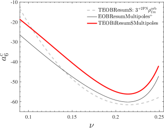
Figure 2: Effective 5PN function $a_{6}^{c}(\nu)$ entering the EOB interaction potential. The previous TEOBResumS function (dashed, grey line) determined in Ref. Nagar et al. (2016) is contrasted with the two new determinations of $a_{6}^{c}$ corresponding to the TEOBiResumMultipoles or to the EOBResumMultipoles⁺ choices. The difference is due to changes in the radiation reaction as well as to the reduced nominal error bars of the NR data used.

IV.0.1 TEOBiResumMultipoles

The best values of $a_{6}^{c}$ determined by EOB/NR phasing comparison are listed in the third column of Table 1. To fit them properly we use the following rational function

$$a_{6}^{c}=n_{0}\dfrac{1+n_{1}\nu+n_{2}\nu^{2}+n_{3}\nu^{3}}{1+d_{1}\nu},$$ (58)

where the parameters are determined to be

$$n_{0} =\;\;\;5.9951,$$ (59)

$$n_{1} =-34.4844,$$ (60)

$$n_{2} =-79.2997,$$ (61)

$$n_{3} =\;\;\;713.4451,$$ (62)

$$d_{1} =-3.167.$$ (63)

IV.0.2 EOBResumMultipoles⁺

With the $3^{+2}$ PN accurate, PN-expanded, version of the $\rho_{\ell m}$’s, the best values of $a_{6}^{c}$ yielding an EOB/NR phase difference compatible with the NR uncertainty are listed in the fourth column of Table 1. These numbers can be accurately fitted with a rational function of the form

$$a_{6}^{c}=n_{0}\dfrac{1+n_{1}\nu+n_{2}\nu^{2}}{1+d_{1}\nu},$$ (64)

where

$$n_{0} =\;\;\;9.3583,$$ (65)

$$n_{1} =-47.4566,$$ (66)

$$n_{2} =\;\;\;162.4461,$$ (67)

$$d_{1} =-3.425.$$ (68)

Table 2: Properties of the 19 non-spinning NR SXS waveforms used to inform the postpeak waveform fits that complete the EOB multipolar waveform. From left to right, the columns report: the identification number; the SXS classification name; the mass ratio $q\equiv m_{1}/m_{2}\geq 1$; the symmetric mass ratio $\nu$; the number of orbits between $t=0$ and the time when a common event horizon is formed; the orbital eccentricity $\epsilon$ determined at relaxed measurement time; the $\ell=m=2$ phase-difference $\delta\phi^{\rm NR}_{\rm mrg}$ between the highest and second highest resolution accumulated between $t=600M$ and the peak amplitude of the highest resolution data; the highest resolution available ${\rm Lev_{h}}$ and the second-highest resolution available ${\rm Lev_{l}}$.

#	name	$q$	$\nu$	$\#$ orbits	$\epsilon\left[10^{-3}\right]$	$\delta\phi^{\rm NR}_{\rm mrg}\left[{\rm rad}\right]$	${\rm Lev_{h}}$	${\rm Lev_{l}}$
$1$	SXS:BBH:0180	$1$	$0.2500$	$28.1825$	$0.0514$	$-0.4247$	Lev4	Lev3
$2$	SXS:BBH:0007	$1.5$	$0.2400$	$29.0922$	$0.4200$	$-0.0186$	Lev6	Lev5
$3$	SXS:BBH:0169	$2$	$0.2222$	$15.6805$	$0.1200$	$-0.0271$	Lev5	Lev4
$4$	SXS:BBH:0259	$2.5$	$0.2041$	$28.5625$	$0.0590$	$-0.0080$	Lev5	Lev4
$5$	SXS:BBH:0030	$3$	$0.1875$	$18.2228$	$2.0100$	$-0.0870$	Lev5	Lev4
$6$	SXS:BBH:0167	$4$	$0.1600$	$15.5908$	$0.0990$	$-0.5165$	Lev5	Lev3
$7$	SXS:BBH:0295	$4.5$	$0.1488$	$27.8067$	$0.0520$	$+0.2397$	Lev5	Lev4
$8$	SXS:BBH:0056	$5$	$0.1389$	$28.8102$	$0.4900$	$+0.4391$	Lev5	Lev4
$9$	SXS:BBH:0296	$5.5$	$0.1302$	$27.9335$	$0.0520$	$+0.4427$	Lev5	Lev4
$10$	SXS:BBH:0166	$6$	$0.1224$	$21.5589$	$0.0440$	…	Lev5	…
$11$	SXS:BBH:0297	$6.5$	$0.1156$	$19.7111$	$0.0640$	$-0.0543$	Lev5	Lev4
$12$	SXS:BBH:0298	$7$	$0.1094$	$19.6757$	$0.0610$	$-0.0775$	Lev5	Lev4
$13$	SXS:BBH:0299	$7.5$	$0.1038$	$20.0941$	$0.0590$	$-0.0498$	Lev5	Lev4
$14$	SXS:BBH:0063	$8$	$0.0988$	$25.8255$	$0.2800$	$+1.0094$	Lev5	Lev4
$15$	SXS:BBH:0300	$8.5$	$0.0942$	$18.6953$	$0.0570$	$-0.0804$	Lev5	Lev4
$16$	SXS:BBH:0301	$9$	$0.0900$	$18.9274$	$0.0550$	$-0.1641$	Lev5	Lev4
$17$	SXS:BBH:0302	$9.5$	$0.0862$	$19.1169$	$0.0600$	$+0.0206$	Lev5	Lev4
$18$	SXS:BBH:0185	$9.99$	$0.0827$	$24.9067$	$0.3055$	$+0.3714$	Lev3	Lev2
$19$	SXS:BBH:0303	$10$	$0.0826$	$19.2666$	$0.0510$	$+0.2955$	Lev5	Lev4

Note that in this case a function with only 4 parameters is sufficient and we didn’t use the $q=7$ data. Figure 2 illustrates the differences between the NR-informed function $a_{6}^{c}(\nu)$ of Eq. 57 from Ref. Nagar et al. (2016), implemented in TEOBResumS, and the two new ones (58)-(64). Two things are noticeable: (i) the need to comply with the rather small error bars in the NR data forces $a_{6}^{c}(\nu)$ to be essentially linear as $\nu\to 0$. Such qualitative behavior is consistent with the analytical expectation, though the $\nu=0$ numerical values obtained from the fits are not. In fact, in one case the limit is $\simeq 6$ and in the other is $\simeq 9$, both very different from the value of $a_{6}^{c}(0)$ known analytically from gravitational self-force (GSF) calculations Barausse et al. (2012); Bini and Damour (2014), $a_{6}^{c}(0)\simeq-134.072$ (see Eq. (67a) of Bini and Damour (2014)). This difference is not surprising seen that (i) our $a_{6}^{c}$ is an effective parameter that enters a Padé approximant and (ii) that it does depend (as we showed) on the analytical choices made to construct the radiation reaction and on the details of the NQC correction factors . Clearly, seen the effective nature of $a_{6}^{c}(\nu)$, the nonspinning models that we are constructing are not expected to give a faithful representation of the true physics for large mass-ratio binaries (e.g. extreme-mass-ratio inspirals) because of the lack of the correct linear-in-$\nu$ analytical information in the interaction potential. Evidently, this is not a conceptual issue, since, in principle, high-order analytical information could be incorporated in the $A$ function that could then be resummed accordingly. A dedicated investigation is needed to assess whether such GSF-augmented $A$ function would improve the agreement with NR data as is or it (still) would need to be additionally informed by some other effective parameter, e.g. like the 5PN coefficient in the $A$ potential proportional to $\nu^{2}$. As a positive final note, we shall check below that our NR-informed determinations of $a_{6}^{c}(\nu)$ are still sufficiently valid for $\nu\simeq 0.0499$ ($q=18$), as they yield an excellent EOB/NR waveform agreement with a (relatively short) $q=18$ NR waveform obtained with the BAM code.

V Multipolar ringdown waveform

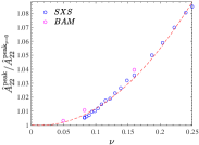
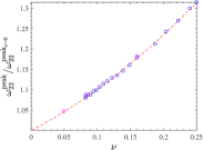
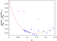
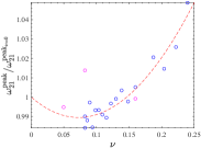
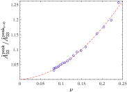
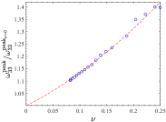
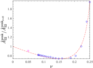
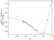
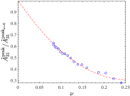
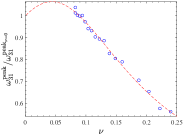
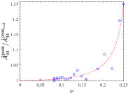
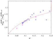
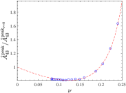
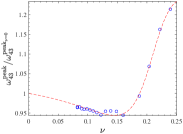
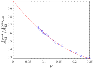
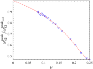
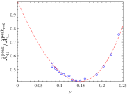
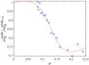
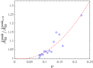
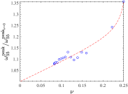
Figure 3: Comparison of orbital fits of peak amplitude and frequency versus SXS and BAM data for the multipoles $\ell\leq 4$, $1\leq m\leq 4$, and $(\ell,m)=(5,5)$.

Table 3: Parameters for the fit of the peak amplitude and frequency of all multipoles up to $\ell=m=5$. From left to right, the columns report: the multipolar indices; the values of the amplitude and frequency in the test-particle limit, $(\hat{A}^{0}_{\ell m},\omega^{0}_{\ell m})$; the amplitude fit coefficients $(n_{i}^{A_{\ell m}},d_{i}^{A_{\ell m}})$ and the frequency fit coefficients $(n_{i}^{\omega_{\ell m}},d_{i}^{\omega_{\ell m}})$ for the functions $(\hat{\hat{A}}_{\ell m},\hat{\omega}_{\ell m})$ defined in Eqs. (85)-(86) and fitted using the rational function template of Eq. (87). Note that since all $d_{2}^{A_{\ell m}}$ values are found to be equal to zero we do not explicitly report them in the table.

$\ell$	$m$	$\hat{A}^{0}_{\ell m}$	$\omega^{0}_{{\ell m}}$	$n_{1}^{A_{\ell m}}$	$n_{2}^{A_{\ell m}}$	$d_{1}^{A_{\ell m}}$	${n}_{1}^{\omega_{\ell m}}$	${n}_{2}^{\omega_{\ell m}}$	${d}_{1}^{\omega_{\ell m}}$	$d_{2}^{\omega_{\ell m}}$
2	2	$0.295896$	$0.273356$	$-0.041285$	$1.5971$	…	$0.84074$	$1.6976$	…	…
	1	$0.106935$	$0.290672$	$9.0912$	$3.9331$	$11.108$	$-0.060432$	$1.9995$	$0.23248$	…
3	3	$0.051670$	$0.454622$	$0.098379$	$3.8179$	…	$1.1054$	$2.2957$	…	…
	2	$0.018168$	$0.451817$	$-6.142$	$11.372$	$-3.6448$	$-9.0214$	$21.078$	$-8.6636$	$19.493$
	1	$0.005694$	$0.411755$	$-5.49$	$10.915$	…	…	$7.5362$	$-2.7555$	$38.572$
4	4	$0.014579$	$0.635415$	$-3.6757$	$0.32156$	$-3.6784$	$3.2876$	$-29.122$	$1.696$	$-22.761$
	3	$0.004962$	$0.636870$	$-5.7791$	$12.589$	$-3.3039$	$-9.0124$	$22.011$	$-8.732$	$20.518$
	2	$0.001656$	$0.626030$	$-4.7096$	$7.3253$	…	$-7.0558$	$12.738$	$-6.0595$	$9.3389$
	1	$0.000487$	$0.552201$	$-8.4449$	$26.825$	$-1.2565$	$-10.876$	$37.904$	$-11.194$	$42.77$
5	5	$0.005227$	$0.818117$	$-0.29628$	$6.4207$	…	$-2.8918$	$-3.2012$	$-3.773$	…

V.1 Overview of the analytical model

The description of the ringdown is based on the model introduced in Ref. Damour and Nagar (2014a) based on a suitable fit of NR waveform data. The original model was improved in Refs. Nagar et al. (2018); Del Pozzo and Nagar (2017) and also adopted, with some modifications, in Ref. Bohé et al. (2017); Cotesta et al. (2018). The idea of Ref. Damour and Nagar (2014a) is to first (i) factorize in the waveform the contribution of the fundamental quasi-normal mode and then (ii) to fit the remaining, time-dependent, complex factor. Here we generalize this procedure, precisely as it was introduced in Damour and Nagar (2014a), to all modes up to $\ell=m=5$. In particular, for each $(\ell,m)$ the fit is done from the peak of each mode. To ease the notation, we define

$$h(\tau)\equiv h_{\ell m}(\tau)\quad\text{with}\quad\tau\geq 0\ ,$$ (69)

where $\tau\equiv(t-t^{\rm peak}_{\ell m})/M_{\rm BH}$, and $M_{\rm BH}$ is the mass of the final BH, computed from the fits of Jiménez-Forteza et al. (2017). In the following we assume that each quantity carries indices ${\ell m}$, that we do not write explictly except when it is needed to avoid confusion. Defining the complex frequency of the fundamental QNM as $\sigma_{1}\equiv\alpha_{1}+{\rm i}\omega_{1}$, the QNM-factorized waveform $\bar{h}(\tau)$ is defined by

$$h\left(\tau\right)=e^{-\sigma_{1}\tau-{\rm i}\phi_{0}}\bar{h}\left(\tau\right).$$ (70)

This is then separated into phase and amplitude as

$$\bar{h}(\tau)=A_{\bar{h}}(\tau)e^{{\rm i}\phi_{\bar{h}}(\tau)},$$ (71)

that are separately fitted using the following ansätze

$$A_{\bar{h}}(\tau)= c_{1}^{A}\tanh\left(c_{2}^{A}\tau+c_{3}^{A}\right)+c_{4}^{A},$$ (72)

$$\phi_{\bar{h}}(\tau)= -c_{1}^{\phi}\mathrm{ln}\left(\frac{1+c_{3}^{\phi}e^{-c_{2}^{\phi}\tau}+c_{4}^{\phi}e^{-2c_{2}^{\phi}\tau}}{1+c_{3}^{\phi}+c_{4}^{\phi}}\right).$$ (73)

However, not all of the coefficients will be free parameters, as we impose five additional constraints so that the fit incorporates the physically correct behavior both at $\tau=0$ and and at late times Damour and Nagar (2014a). Imposing these conditions yields

$$c_{2}^{A}= \frac{1}{2}\alpha_{21},$$ (74)

$$c_{4}^{A}= \hat{A}^{\rm peak}-c_{1}^{A}\tanh\left(c_{3}^{A}\right),$$ (75)

$$c_{1}^{A}= \hat{A}^{\rm peak}\alpha_{1}\frac{\cosh^{2}\left(c_{3}^{A}\right)}{c_{2}^{A}},$$ (76)

$$c_{1}^{\phi}= \Delta\omega\frac{1+c_{3}^{\phi}+c_{4}^{\phi}}{c_{2}^{\phi}\left(c_{3}^{\phi}+2c_{4}^{\phi}\right)},$$ (77)

$$c_{2}^{\phi}= \alpha_{21},$$ (78)

with $\Delta\omega=\omega_{1}-M_{\rm BH}\omega^{\rm peak}$, $\hat{A}^{\rm peak}$ is the value of the multipole amplitude at its peak, as defined in Eq. (84) below (with the $\ell,m$ dependence explicit), and $\alpha_{21}\equiv\alpha_{2}-\alpha_{1}$, i.e. the difference between the inverse damping times of the first overtone ($\alpha_{2}$) and of the fundamental mode $(\alpha_{1})$. The three remaining parameters, $\left(c_{3}^{A},c_{3}^{\phi},c_{4}^{\phi}\right)$, that are the only genuine free parameters of the model, are then fitted directly for any NR dataset. We then define two kind of fits: (i) we address as primary the fit of $(c_{3}^{A},c_{3}^{\phi},c_{4}^{\phi})$ for a given SXS dataset; (ii) we then call as global interpolating fit the one of the coefficients above performed all over the available NR datasets. Let us highlight a few points.

1. For each mode, one needs accurate fits of the amplitude and frequency at the peak of each multipole. Capturing these numbers properly is crucial to accurately reproduce the global post-peak evolution of frequency and amplitude.

2. The QNM information can be fitted with extreme precision against the dimensionless spin $\hat{a}_{f}$ of the final BH. In practice $\hat{a}_{f}$ is determined from the fit presented in Jiménez-Forteza et al. (2017).

3. The effective post-merger parameters $(c_{3}^{A},c_{3}^{\phi},c_{4}^{\phi})$ are very sensitive to noise in the NR waveform and thus extreme precision is not advisable. On the other hand they only sub-dominantly impact the waveform.

4. The primary fitting template given in Eq. (72) does not have enough analytical flexibility to accurately fit the waveform amplitude in the extreme-mass-ratio limit and will have to be changed in order to fully extend the validity of the model to that regime.

V.2 Numerical Relativity Data

We use 19 SXS waveforms Mroue et al. (2013); Chu et al. (2016); Blackman et al. (2015); SXS , summarized in Table 2, and a single test-particle waveform to perform the fits. The details of the waveform generation of the latter and further details can be found here Harms et al. (2014); Nagar and Shah (2016). Several quantities characterizing the waveforms are detailed in Table 2. Most of these are defined in the main text or can be extracted from the ${\tt metadata.txt}$ available online SXS . The only additional quantity that is routinely used to conservatively assess the accuracy of the waveform is the accumulated phase difference between the highest and second-highest resolution up to the peak of the $\ell=m=2$ waveform, that corresponds to the merger of the two objects. The waveforms cover the range $1\leq q\leq 10$, corresponding to $0.08\lesssim\nu\lesssim 0.25$. The waveforms are between $15.5$ and $29.1$ cycles long and have eccentricities never exceeding $\epsilon\approx 2.1\times 10^{-3}$. For most waveforms, $|\delta\phi^{\rm NR}_{\rm mrg}|\lesssim 0.5~{}{\rm rad}$ with the exception of SXS:BBH:0063 which reaches $\delta\phi^{\rm NR}_{\rm mrg}\approx 1~{}{\rm rad}$ which is still an exceptable margin of error.

V.3 Fits: waveform peak frequency and amplitude.

Table 4: Fit coefficients of the postpeak functions $(c_{3}^{A_{\ell m}},c_{3}^{\phi_{\ell m}},c_{4}^{\phi_{\ell m}})$ entering Eqs. (72)-(73). Note the rather special functional form needed for $c_{3}^{A_{32}}$ and $c_{3}^{A_{44}}$, that is necessary to properly account for nearly equal-mass data. In addition, the fits of some multipoles are discontinuous, the interface between the branches being at mass ratios $q=2.5$ or $q=10$. Such mass ratios correspond to the values $\nu=10/49$ and $\nu=10/121$ that appear in the argument of the $\theta$ functions.

$\ell$	$m$	$c_{3}^{A_{\ell m}}$	$c_{3}^{\phi_{\ell m}}$	$c_{4}^{\phi_{\ell m}}$
2	2	$-0.56187+0.75497\nu$	$\frac{4.4414-63.107\nu+296.64\nu^{2}}{1-13.299\nu+69.129\nu^{2}}$	$\frac{7.1508-109.47\nu}{1+556.34\nu+287.42\nu^{2}}$
2	1	$\frac{0.23882-2.2982\nu+5.7022\nu^{2}}{1-7.7463\nu+27.266\nu^{2}}$	$\frac{2.6269-37.677\nu+181.61\nu^{2}}{1-16.082\nu+89.836\nu^{2}}$	$\frac{4.355-53.763\nu+188.06\nu^{2}}{1-18.427\nu+147.16\nu^{2}}$
3	3	$-0.39337+0.93118\nu$	$3.1017-6.5849\nu$	$\frac{3.4521-24.153\nu+53.029\nu^{2}}{1+3.1413\nu}$
3	2	$\frac{0.1877-3.0017\nu+19.501\nu^{2}}{1-1.8199\nu}-e^{-703.67(\nu-2/9)^{2}}$	$\frac{0.90944-1.8924\nu+3.6848\nu^{2}}{1-8.9739\nu+21.024\nu^{2}}$	$\frac{2.3038-50.79\nu+334.41\nu^{2}}{1-18.326\nu+99.54\nu^{2}}$
3	1	$\frac{3.5042-55.171\nu+217\nu^{2}}{1-15.749\nu+605.17\nu^{3}}$	$\frac{-6.1719+29.617\nu+254.24\nu^{2}}{1-1.5435\nu}\theta\left(\nu-\frac{10}{121}\right)$	$3.6485+5.4536\nu$
			$\;\;\;\;\;\;-2.2784\ \theta\left(\frac{10}{121}-\nu\right)$
4	4	$-0.25808+0.84605\nu+1.2376e^{-6054.7(\nu-10/49)^{2}}$	$\frac{2.3328-9.4841\nu+19.719\nu^{2}}{1-2.904\nu}$	$0.94564+3.2761\nu$
4	3	$\frac{-0.02833+2.8738\nu-31.503\nu^{2}+93.513\nu^{3}}{1-10.051\nu+156.14\nu^{3}}$	$\frac{2.284-23.817\nu+70.952\nu^{2}}{1-10.909\nu+30.723\nu^{2}}$	$\frac{2.4966-6.2043\nu}{1-252.47\nu^{4}}$
4	2	$\frac{0.27143-2.2629\nu+4.6249\nu^{2}}{1-7.6762\nu+15.117\nu^{2}}$	$\frac{2.2065-17.629\nu+65.372\nu^{2}}{1-4.7744\nu+3.1876\nu^{2}}$	Eq. (88)
4	1	$11.47+10.936\nu$	$(-6.0286+46.632\nu)\theta\left(\nu-\frac{10}{121}\right)$	$1.6629+11.497\nu$
			$\;\;\;\;\;\;-2.1747\ \theta\left(\frac{10}{121}-\nu\right)$
5	5	$\frac{-0.19751+3.607\nu-14.898\nu^{2}}{1-20.046\nu+108.42\nu^{2}}$	$0.83326+10.945\nu$	$\frac{0.45082-9.5961\nu+52.88\nu^{2}}{1-19.808\nu+99.078\nu^{2}}$

Let us turn now to discussing the fits of amplitude and frequency at each multipole peak. For consistency with previous work, we shall use from now on the Regge-Wheeler-Zerilli normalized Nagar and Rezzolla (2005) strain waveform

$$\Psi_{\ell m}\equiv h_{\ell m}/\sqrt{(\ell+2)(\ell+1)\ell(\ell-1)},$$ (79)

so that the multipolar waveform is separated in amplitude and phase as

$$\Psi_{\ell m}=A_{\ell m}e^{-{\rm i}\phi_{\ell m}},$$ (80)

and the frequency is $\omega_{\ell m}=\dot{\phi}_{\ell m}$. We then define $t^{\rm peak}_{\ell m}$ as the time where each $A_{{\ell m}}$ peaks, i.e. $\dot{A}_{\ell m}(t_{\rm peak})=0$ and then we measure the values of amplitude and frequency at $t_{\rm peak}$, $(A_{\ell m}^{\rm peak},\omega_{\ell m}^{\rm peak})$. We hence define

$$\omega_{\ell m}^{\rm peak} \equiv\omega_{\ell m}(t)|_{t=t_{\ell m}^{\rm peak}},$$ (81)

$$A^{\rm peak}_{\ell m} \equiv A_{\ell m}(t)|_{t=t_{\ell m}^{\rm peak}}.$$ (82)

To build analytical fits of $(A_{\ell m}^{\rm peak},\omega_{\ell m}^{\rm peak})$ we proceed as follows. First, we factor out from the peak values the leading-order $\nu$ behavior. This is given by the function

$$c_{\ell+\epsilon}(\nu)=X_{2}^{\ell+\epsilon-1}+(-)^{\ell+\epsilon}X_{1}^{\ell+\epsilon-1}$$ (83)

and we define

$$\hat{A}_{{\ell m}}\equiv A_{\ell m}/c_{\ell+\epsilon}(\nu)\ .$$ (84)

As a second step, we also factor out the the test-particle values $(\hat{A}_{\ell m}^{0},\omega_{\ell m}^{0})$, that are known with high accuracy (see Table 3 of Ref. Harms et al. (2014)). In pratice, the quantities to be fitted are $(\hat{\hat{A}}^{\rm peak}_{\ell m},\hat{\omega}_{\ell m}^{\rm peak})$ defined as

$$A^{\rm peak}_{\ell m} =c_{\ell+\epsilon}(\nu)\hat{A}^{\rm 0}_{\ell m}\hat{\hat{A}}^{\rm peak}_{\ell m},$$ (85)

$$\omega^{\rm peak}_{\ell m} =\omega^{\rm 0}_{\ell m}\hat{\omega}^{\rm peak}_{\ell m}.$$ (86)

Figure 3 illustrates the behavior of the NR quantities $(\hat{\hat{A}}_{\ell m},\hat{\omega}_{\ell m})$ versus $\nu$. Whenever possible, we show together SXS and BAM datapoints to illustrate the consistency between results obtained with very different computational infrastructures. One finds that the datapoints can be easily fitted with a rational function with the general form

$$f_{\ell m}=\frac{1+n_{1}^{f_{\ell m}}\nu+n_{2}^{f_{\ell m}}\nu^{2}}{1+d_{1}^{f_{\ell m}}\nu+d_{2}^{f_{\ell m}}\nu^{2}},$$ (87)

where $f_{\ell m}$ is either $\hat{\hat{A}}_{\ell m}^{\rm peak}$ or $\hat{\omega}_{\ell m}^{\rm peak}$. The fit coefficients are listed in Table 3. All fits have been done with fitnlm of MATLAB. The coefficients were set to zero by default if fitnlm returned a significant p-value, i.e. $\gtrapprox 0.3$.

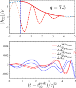
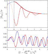
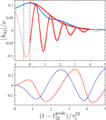
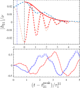
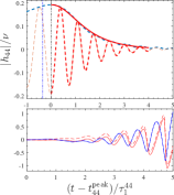
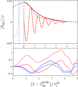
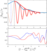
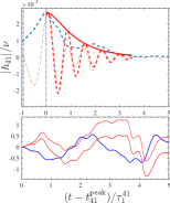
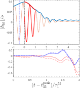
Figure 4: Performance of the primary postpeak fit and and of the global interpolating fit on dataset SXS:BBH:0299 with mass ratio $q=7.5$. We here consider the modes $(\ell,m)=(2,2),(2,1),(3,3),(3,2),(3,1),(4,4),(4,3),(4,2),(4,1)$ and $(5,5)$. The panel of each mode is divided into two subpanels. In the top one, the tick-red lines represent the waveform (amplitude, solid, and real part, dashed) obtained evaluating the primary fit of the parameters of Eqs. (72)-(73). By contrast, the thin orange line is the real part of the NR waveform, while the corresponding modulus is depicted as a blue, dashed, thick line. The vertical line in black marks $t_{\rm peak}^{{\ell m}}$, while the blue one is $t_{22}^{\rm peak}$. For each mode, the time $t-t_{{\ell m}}^{\rm peak}$ is expressed in units of $\tau_{1}^{{\ell m}}\equiv 1/\alpha_{1}^{{\ell m}}$, the damping time of the corresponding $(\ell,m)$ fundamental QNM. In the bottom subpanel we show the phase difference between the NR and the fit for the phase (red online) and the fractional amplitude difference (blue online). The differences with the primary fit are shown as solid lines, while those with the the global, interpolating, fit as dashed lines. One sees a more than acceptable consistency between the performances of the two fits.

V.4 Fits: postpeak waveform and ringdown

As mentioned above, for the postpeak multipolar waveform we adopt a 2-step fitting procedure: (i) for each NR dataset considered, we perform a primary fit, to determine the parameters $(c_{3}^{A_{\ell m}},c_{3}^{\phi_{\ell m}},c_{4}^{\phi_{\ell m}})$ that describe the postpeak behavior for each NR waveform at our disposal; then (ii) these parameters are fitted versus $\nu$ to get the global interpolating fits. The $\ell=m=2$ postpeak fits are informed using all the 19 datasets in Table 2. By contrast, only subsamples are used for the higher modes, depending on the accuracy of the corresponding waveform. More precisely we use the following datasets (numbering follows Table 2):$\{2-16,18,19\}$ for $(2,1)$; $\{2-19\}$ for $(3,3)$; $\{1-15,17,18\}$ for $(3,2)$; $\{2-11,13,14,17,18\}$ for $(3,1)$; $\{1-11,13,15-19\}$ for $(4,4)$; $\{2-9,13-19\}$ for $(4,3)$; $\{1-8,10-14,17-18\}$ for $(4,2)$ and $\{3,6,9-19\}$ for $(5,5)$. For each $(\ell,m)$, the primary fit is always performed over a time interval $\Delta\tau_{\ell m}$. We choose $\Delta\tau_{\ell m}=4\tau^{\ell m}_{1}=4/\alpha^{\ell m}_{1}$ for $\ell=m=2$ as well as for all other multipoles (except $\ell=m=5$) for datesets $\{10-19\}$ (corresponding to $q\geq 6$). For datasets $\{1-9\}$(corresponding to $q\leq 5.5$) and for the $\ell=m=5$ mode all over, we use $\Delta\tau_{\ell m}=\tau^{\ell m}_{1}$. This choice was partly driven by data-quality issues and partly by the presence of mode mixing (see bottom, right panel of Fig. 4 as an example of the data-quality issues in the $(5,5)$ mode). The performances of both the primary and global fits are illustrated in Fig. 4, that refers to the illustrative dataset SXS:BBH:0299, with $q=7.5$. For this specific comparison we are plotting $h_{\ell m}/\nu$ instead of $\Psi_{\ell m}$. For convenience, for each $(\ell,m)$, time is expressed using the variable $(t-t_{\ell m}^{\rm peak})/\tau_{1}^{\ell m}$. As mentioned above, the rightmost, bottom, panel of the figure illustrates how the numerical noise shows up already at $t-t_{55}^{\rm peak}\approx\tau^{55}_{1}$. The temporal interval where the primary fit is performed is highlighted with the thick-red lines (solid for the modulus, dashed for the real part) in the top part of each panel. The fact that our post-peak templates lacks, by design, of the possibility of accommodating any type of mode mixing results apparent from inspecting the figure (especially the amplitude and phase differences, that are displayed in the bottom part of each panel). For example, it is well known that the ringdown part of the $(2,1)$ modes is mostly represented by a superposition of the fundamental modes with $\sigma^{\pm}_{1}=\alpha^{21}_{1}\pm{\rm i}\omega^{21}_{1}$; similarly, the $(3,2)$ multipole incorporates both the $\ell=2$, $m=2$ and $\ell=3$, $m=2$ QNMs frequencies of the final black hole [similar considerations hold for $(3,1)$, $(4,3)$ and $(4,2)$] because the waveform is expanded in spin-weighted spherical harmonics and not along the basis of the spheroidal harmonics that is naturally associated to the finally formed black hole. The lack of modelization of this effect is responsible of the fact that, for these modes, the fit residuals show a constant-amplitude oscillation, instead of being (essentially) flat as they are supposed to be in the case of the $\ell=m$ modes, where the effect of mode mixing is usually largely suppressed (though it may increase with the mass ratio, see Ref. Bernuzzi and Nagar (2010)). Note however that the corresponding plots are still showing oscillations that grow with time. This effect mostly comes from numerical noise that gets amplified by the radius-extrapolation procedure. We also need to highlight that in the bottom part of each panel we show both the residuals with the primary fits (solid lines) and with the global interpolating fits (dashed lines). The plot proves, on average, a more than acceptable consistency and reliability of the global interpolating fit. In conclusion, the postmerger template we are using here gives a simple and effective, although certainly physically incomplete, representation of the actual physics. We shall assess below the influence of this approximation on standard measures of merit.

Table 5: Parameters of the fitting function given by Eq. (89) used to fit the QNM parameters entering the phenomenological description of the postmerger waveform. We list here the fundamental QNM frequency $\omega^{\ell m}_{1}$ and (inverse) damping time $\alpha_{1}^{\ell m}$ as well as the difference $\alpha_{21}^{\ell m}=\alpha^{\ell m}_{2}-\alpha^{\ell m}_{1}$.

${Y^{\prime}}$	$\ell$	$m$	${Y^{\prime}}_{0}$	$b^{Y^{\prime}}_{1}$	$b^{Y^{\prime}}_{2}$	$b^{Y^{\prime}}_{3}$	$c^{Y^{\prime}}_{1}$	$c^{Y^{\prime}}_{2}$	$c^{Y^{\prime}}_{3}$
$\omega_{1}^{\ell m}$	2	2	$0.373672$	$-1.5367$	$0.5503$	…	$-1.8700$	$0.9848$	$-0.10943$
		1	$0.373672$	$-0.79546$	$-0.1908$	$0.11460$	$-0.96337$	$-0.1495$	$0.19522$
	3	3	$0.599443$	$-1.84922$	$0.9294$	$-0.07613$	$-2.18719$	$1.4903$	$-0.3014$
	3	2	$0.599443$	$-0.251$	$-0.891$	$0.2706$	$-0.475$	$-0.911$	$+0.4609$
	3	1	$0.599443$	$-0.70941$	$-0.16975$	$0.08559$	$-0.82174$	$-0.16792$	$0.14524$
	4	4	$0.809178$	$-1.83156$	$0.9016$	$-0.06579$	$-2.17745$	$1.4753$	$-0.2961$
	4	3	$0.809178$	$-1.8397$	$0.9616$	$-0.11339$	$-2.0979$	$1.3701$	$-0.2675$
	4	2	$0.0941640$	$-1.44152$	$0.0542$	$0.39020$	$-1.43312$	$0.1167$	$0.32253$
		1	$0.0941640$	$1.1018882$	$-0.88643$	$-0.78266$	$1.1065495$	$-0.80961$	$-0.68905$
$\alpha_{1}^{\ell m}$	2	2	$0.08896$	$-1.90036$	$0.86200$	$0.0384893$	$-1.87933$	$0.88062$	…
		1	$0.0889623$	$-1.31253$	$-0.21033$	$0.52502$	$-1.30041$	$-0.1566$	$0.46204$
	3	3	$0.0927030$	$-1.8310$	$0.7568$	$0.0745$	$-1.8098$	$0.7926$	$0.0196$
		2	$0.0927030$	$-1.58277$	$0.2783$	$0.30503$	$-1.56797$	$0.3290$	$0.24155$
		1	$0.0927030$	$-1.2345$	$-0.30447$	$0.5446$	$-1.2263$	$-0.24223$	$0.47738$
	4	4	$0.0941640$	$-1.8662$	$0.8248$	$0.0417$	$-1.8514$	$0.8736$	$-0.0198$
		3	$0.0941640$	$-1.7177$	$0.5320$	$0.1860$	$-1.7065$	$0.5876$	$0.120939$
		2	$0.190170$	$-1.38840$	…	$0.39333$	$-1.37584$	$0.0600017$	$0.32632$
		1	$0.190170$	$1.0590157$	$-0.8650630$	$-0.75222$	$1.0654880$	$-0.7830051$	$-0.65814$
$\alpha_{21}^{\ell m}$	2	2	$0.184953$	$-1.89397$	$0.88126$	$0.0130256$	$-1.83901$	$0.84162$	…
		1	$0.184952$	$-1.1329$	$-0.3520$	$0.4924$	$-1.10334$	$-0.3037$	$0.4262$
	3	3	$0.188595$	$-1.8011$	$0.7046$	$0.0968$	$-1.7653$	$0.7176$	$0.0504$
		2	$0.188595$	$-1.5212$	$0.1563$	$0.3652$	$-1.4968$	$0.1968$	$0.3021$
		1	$0.188595$	$-1.035$	$-0.3816$	$0.4486$	$-1.023$	$-0.3170$	$0.3898$
	4	4	$0.190170$	$-1.8546$	$0.8041$	$0.0507$	$-1.8315$	$0.8391$	$-0.0051$
		3	$0.190170$	$-1.6860$	$0.4724$	$0.2139$	$-1.6684$	$0.5198$	$0.1508$
		2	$0.809178$	$-0.6644$	$-0.3357$	$0.1425$	$-0.8366$	$-0.2921$	$0.2254$
		1	$0.809178$	$-0.68647$	$-0.1852590$	$0.0934997$	$-0.77272$	$-0.1986852$	$0.1485093$

Table 6: The fit parameters to analytically represent the time lag between the peak of the $(\ell,m)$ waveform multipole and the peak of the $(2,2)$ mode, Eq. (90). The coefficients refer to the functional form of Eqs. (91)-(92).

$\ell$	$m$	$\Delta t^{\rm 0}_{\ell m}$	$n_{1}^{\Delta t_{{\ell m}}}$	$n_{2}^{\Delta t_{\ell m}}$	${d}_{1}^{\Delta t_{\ell m}}$	$d_{2}^{\Delta t_{\ell m}}$
2	1	$11.7900$	$-3.764$	$6.9051$	…	…
3	3	$3.49238$	$-0.11298$	$5.0056$	…	…
3	2	$9.22687$	$-11.398$	$33.244$	$-8.1976$	$19.537$
3	1	$12.9338$	…	$-25.615$	$0.88803$	$16.292$
4	4	$5.28280$	$-8.4686$	$18.006$	$-6.7964$	$11.368$
4	3	$9.59669$	$-11.345$	$38.813$	$-7.5049$	$22.399$
4	2	$11.9225$	$-3.8284$	$-12.399$	…	…
4	1	$13.1116$	$-9.6225$	$38.451$	$-7.7998$	$32.405$
5	5	$6.561811$	$-12.198$	$40.327$	$-11.501$	$39.431$

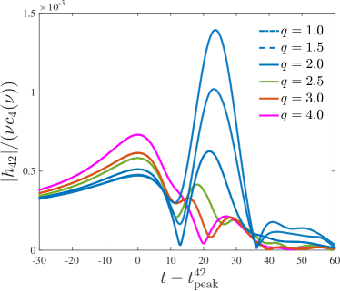
Figure 5: NR data for $q=7.5$: behavior of the post-peak amplitude for $(4,2)$, with a large secondary peak due to mode-mixing.

The fits of $(c_{3}^{A_{\ell m}},c_{3}^{\phi_{\ell m}},c_{4}^{\phi_{\ell m}})$ were obtained using the function fitnlm of MATLAB. The functional form of the fitting function was adapted multipole by multipole, so to have enough flexibility to reduce as much as possible the differences in phase and amplitude, without, however, overfitting the data. We mostly use rational functions that are explicitly listed in Table 4. Inspecting the table, one notes that the derivatives with respect to $\nu$ of $c_{3}^{\phi_{31}}$ and of $c_{3}^{\phi_{41}}$ are discontinuous at $\nu=10/121$ (corresponding to $q=10$). Similarly, the derivative with respect to $\nu$ for $c_{4}^{\phi_{42}}$ turns out to be discontinuous at both $\nu=10/49$ (i.e. $q=2.5$) and at $\nu=3/16$ (i.e. $q=3$) as it turned out convenient to have it represented by the following piece-wise function

$$\!\!\!\frac{132.56-1155.5\nu+2516.8\nu^{2}}{1-3.8231\nu} \qquad\text{if}\quad q\leq 2.5,$$

$$\!\!\!-554.18\nu+120.23 \qquad\text{if}\quad 2.5<q<3,$$ (88)

$$\!\!\!\frac{-0.58736+16.401\nu}{1-4.5202\nu} \qquad\text{if}\quad q\geq 3.$$

The need of such functional representation is related to our approximation of neglecting mode-mixing effects, whose impact depends on the mass ratio. Indeed, one finds (see the illustrative Fig. 5) that the qualitative features of the $(4,2)$ multipole in the range $1\leq q\leq 2.5$ are peculiar: the postmerger waveform amplitude has a double-peaked structure due to mode-mixing, and in this range of mass ratios the amplitude of the second peak is larger than that of the first one. The lowering of the second peak is rather abrupt with the mass ratio and occurs somewhere in the interval $2<q<2.5$, where we do not have additional NR simulations. Although such feature is nothing more than an artifact related to having expressed the waveform in the basis of spherical harmonics (instead of the natural spheroidal one), it is just approximately represented by our, rather simplified, fit.

We also need fits of the QNMs quantities $(\omega^{\ell m}_{1},\alpha^{\ell m}_{1})$ and $\alpha_{21}^{\ell m}\equiv\alpha_{2}^{\ell m}-\alpha_{1}^{\ell m}$ for all multipoles considered. Each of these parameters is represented as a function of the dimensionless spin of the final black hole, $\hat{a}_{f}$, that reads

$${Y^{\prime}}_{\ell m}\left(\hat{a}_{f}\right)={Y^{\prime}}_{0}\,\frac{1+b_{1}^{Y^{\prime}}\hat{a}_{f}+b_{2}^{Y^{\prime}}\hat{a}_{f}^{2}+b_{3}^{Y^{\prime}}\hat{a}_{f}^{3}}{1+c_{1}^{Y^{\prime}}\hat{a}_{f}+c_{2}^{Y^{\prime}}\hat{a}_{f}^{2}+c_{3}^{Y^{\prime}}\hat{a}_{f}^{3}}.$$ (89)

The values of $(\alpha^{\ell m}_{1},\omega_{1}^{\ell m},\alpha_{21}^{\ell m})$ to be fitted were obtained as follows: first, we computed the value of the final spin $\hat{a}_{f}$ using the NR-informed fit presented in Jiménez-Forteza et al. (2017); then, we interpolated the tables of Ref. Berti et al. (2006). The coefficients of the fits above are collected in Table 5. All fits were done with fitnlm of MATLAB and coefficients have been set to zero explicitly if the p-value was significant.

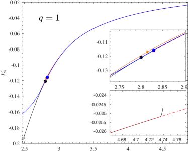
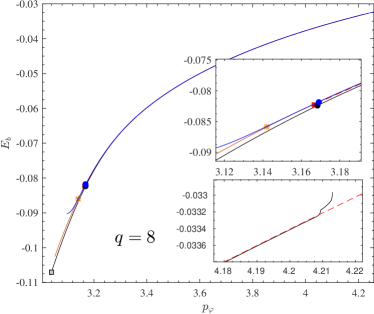
Figure 6: Energetics: comparison between three different EOB models and the SXS NR data computed in Ref. Nagar et al. (2016) for two different binary configurations with mass ratio $q=1$ and $q=8$. Blue line: TEOBiResumMultipoles; Red (dashed) line: the TEOBResumS model of Ref. Nagar et al. (2016) with $a_{6}^{c}(\nu)$ given by Eq. (57); Orange line: SEOBNRv4; black line, NR curve. The filled markers indicate the merger points. The figure highlights the consistency between the two avatars of the TEOBResumS model. Note that the discrepancy between SEOBNRv4 and the NR curve is much larger than the numerical uncertainty on the curve Damour et al. (2012); Nagar et al. (2016).

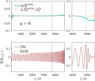
Figure 7: Illustrative EOB/NR time-domain comparison for $q=6$ (corresponding to SXS:BBH:0166) using TEOBiResumMultipoles. Top row: phase difference and relative amplitude differences. Bottom row: comparison between the real part of the waveform.

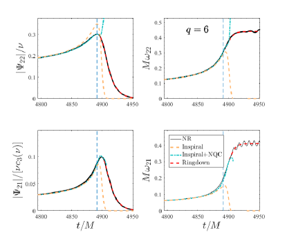
Figure 8: Mass ratio $q=6$, SXS:BBH:0166. Complement to the phasing comparison of Fig. 7: frequency and amplitude for $(2,2)$ (top) and $(2,1)$ (bottom) multipoles obtained with TEOBiResumMultipoles. Orange (dashed) lines: purely analytical EOB waveform ($\hat{h}_{{\ell m}}^{\rm NQC}=1$). Blue lines: NQC-improved waveform with NQC parameters determined by matching to a single NR waveform point. Red lines: postpeak-ringdown part. Vertical line: location of the peak of the $(2,2)$ mode. Mode-mixing is not incorporated in the analytical ringdown description, so the EOB frequency for the $(2,1)$ mode saturates to the plateau and, differently from the numerical one, does not exhibit any oscillation. Note the rather accurate representation of the frequency and amplitude already achievable, essentially up to merger, using the purely analytical (non-NQC corrected), EOB waveform.

The last step required to complete the postmerger model is to extract, from the NR simulations, the time lag, as a function of $\nu$, between the peak of each multipolar mode and the $(2,2)$ one, i.e.

$$\Delta t_{\ell m}^{\rm NR}=t_{\ell m}^{\rm peak}-t_{22}^{\rm peak}.$$ (90)

To represent this as function of $\nu$, as usual we factor out the test-particle values $\Delta t_{\ell m}^{0}$ (see Table 3 of Ref. Harms et al. (2014)), as

$$\Delta t_{\ell m}^{\rm NR}=\Delta t^{0}_{\ell m}\hat{\Delta}t_{\ell m},$$ (91)

and fit the correction $\hat{\Delta}t_{\ell m}$ versus $\nu$. The fits are done with the following, general, functional form

$$\hat{\Delta}t_{\ell m}=\frac{1+n_{1}^{\Delta t_{\ell m}}\nu+n_{2}^{\Delta t_{\ell m}}\nu^{2}}{1+d^{\Delta t_{\ell m}}_{1}\nu+d^{\Delta t_{\ell m}}_{2}\nu^{2}}.$$ (92)

The coefficients of the fits, together with the values of $\Delta t_{\ell m}^{0}$, are listed in Table 6. The fits have been done with fitnlm of MATLAB. Coefficients have been set to zero explicitly if the p-value was significant.

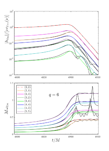
Figure 9: Mass ratio $q=6$, SXS:BBH:0166 dataset (black lines). EOB/NR comparison between amplitudes $|h_{\ell m}(t)|$ (top panel) and frequencies $\omega_{\ell m}(t)$ (bottom panel). For readability, here the modes have been normalized by $\nu c_{\ell+\epsilon}(\nu)$.

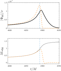
Figure 10: Mass ratio $q=6$, SXS:BBH:0166. Performance of the bare EOB waveform amplitude and frequency (without NQC factor and post-peak description), orange, dashed lines, for the subdominant $\ell=5$ multipoles and for $\ell=m=6$. The solid, black, lines are the NR multipoles. The vertical line in each panel marks the location of the $\ell=m=2$ waveform peak, i.e. the merger. It is remarkable the EOB/NR good agreement between frequencies up to the merger points, especially for the multipoles with the largest values of $m$.

VI Energetics

Now that we have discussed all the building blocks of our nonspinning waveform model(s), let us turn to discussing its performance towards all the available NR data. To simplify the discussion, we focus only on TEOBiResumMultipoles, as it will serve, in a forthcoming study, as baseline for constructing a multipolar waveform model for spin-aligned binaries. In this section, we briefly discuss the energetics of the model. We do this by means of the gauge-invariant relation between the binding energy and angular momentum computed both from NR data and in TEOBiResumMultipoles. This analysis was extensively done already for previous versions of our EOB model Damour et al. (2012); Nagar et al. (2016) and more recently also for the SEOBNRv4 model Ossokine et al. (2018). As an illustrative example, we focus Fig. 6 on the case of two mass ratios, $q=1$ and $q=8$, where $E_{b}\equiv(E-M)/\mu$ is the binding energy per unit mass. For the EOB case, one has $E\equiv\mu\hat{H}_{\rm EOB}$ computed along the EOB dynamics. The NR curves (black online) are precisely those obtained in Ref. Nagar et al. (2016), to which we refer the reader for additional details. The curves obtained with TEOBiResumMultipoles are shown in blue, while those of the EOB model of  Nagar et al. (2016) (i.e., TEOBResumS as in Ref. Nagar et al. (2018)) in red. The figure illustrates the excellent mutual consistency between the two models despite the modifications in the radiation reaction and in the determination of $a_{6}^{c}(\nu)$. The location of the merger is indicated by the markers, of the same color of the corresponding line. Note that the TEOBiResumMultipoles curves are extended also after the merger, but should not be trusted there, as they are obtained from the pure relative dynamics augmented with the NQC factor that is not trustable after the NQC point. Moreover, the ringdown losses are not included in these curves. The correct extension of the EOB $E_{b}(p_{\varphi})$ curve beyond merger requires these details to be taken into account and is postponed to future work. Finally, in the same figure we also show, as orange lines, the $E_{b}(p_{\varphi})$ curves obtained from SEOBNRv4 Bohé et al. (2017). Note that, despite this model being publicly available through the LIGO LALSuite LIGO Scientific Collaboration (2018) library, the corresponding code is not giving, by default, the evolution of the dynamics. Similarly to Ossokine et al. (2018), we modified the code in function XLALSimIMRSpinAlignedEOBModes, contained in LALSimIMRSpinAlignedEOB.c, in order to have access to this information. In particular we were able to obtain an additional output file, containing the full dynamics $(t,r,\varphi,p_{r_{*}},p_{\varphi},M\Omega,E)$, when calling lalsim-inspiral from command line. Then, exploiting the waveform generated by lalsim-inspiral itself, we computed the waveform amplitude, identified the merger time $t_{\rm mrg}$ corresponding to the amplitude peak, and finally found $E_{b}^{\rm mrg}\equiv E_{b}(t_{\rm mrg})$ and $p_{\varphi}^{\rm mrg}=p_{\varphi}(t_{\rm mrg})$. The changes made to LALSuite’s source code, together with the data needed to reproduce Fig. 6, are publicly available at Gamba . Inspecting the top and bottom panel of Fig. 6, and in particular the insets, we conclude that: (i) for $q=1$, SEOBNRv4 seems to overestimate the binding energy during the late stages of the dynamics up to merger of about $1\%$. Note that, although this looks like an acceptably small number, it is actually larger than the numerical uncertainty on the curve Damour et al. (2012); Nagar et al. (2016). By contrast, (ii) when $q=8$ the various curves look more consistent among themselves, although the SEOBNRv4 prediction of the merger values is significantly different from either the NR or the TEOBResumS/TEOBiResumMultipoles values. We postpone to future investigations a detailed understanding of the origin of these features of SEOBNRv4.

VII Phasing analysis

VII.1 Time-domain phasing analysis

Let us move now to assessing the quality of the multipolar waveform. We do so by looking at the usual EOB/NR phase differences as well as at comparisons between frequency and amplitudes for the various multipoles. As for the case of energetics discussed above, we focus only on waveforms generated by TEOBiResumMultipoles. Aim of this section is to demonstrate the following points: (i) the rather remarkable agreement between frequency and amplitude, for all multipoles, that can be accomplished already with the bare EOB waveform, even without the NQC correction factors; (ii) the (rather small) effect brought by NQC corrections, that is more important on the amplitude than on the frequency; (iii) the fact that the transition to the ringdown (or postpeak) phase can be done consistently multipole by multipole, in the sense that the same procedure can be applied on each mode once the relevant NR information is taken into account and properly represented; (iv) accurate description of the postpeak-ringdown phase that is robust and reliable, though still without mode mixing. We highlight this by selecting a specific EOB/NR comparison done for $q=6$, that corresponds to SXS:BBH:0166.

Figure 11: Unfaithfulness between the TEOBiResumMultipoles model and SXS:0303, a binary of mass ratio $q=10$, assuming a total mass of $M=100M_{\odot}$ using the Advanced LIGO and Virgo design sensitivity PSD (zerodethp). The left plot shows the unfaithfulness between EOB and NR using a subset of the most prominent modes: $\{22,21,33,44,55\}$. The right plot shows the degredation in the unfaithfulness from using just the dominant 22-mode in the model. As expected, the unfaithfulness degrades as we approach edge-on systems where the relative contribution of higher modes becomes more pronounced.

Figure 7 illustrates the (rather good) time-domain phasing agreement between the $\ell=m=2$ EOB and NR modes. From Table 2 we see that this dataset was simulated at one single resolution from the SXS collaboration, so that a specific estimate of its error bar at merger is not possible. We may however imagine that it is of the order of the $q=6.5$ simulation, that has approximately the same number of orbits and that starts at approximately the same frequency ($M\omega_{0}\simeq 0.020$), i.e. $\sim-0.05$ rad at merger. This value is compatible with the EOB-NR phase difference at merger that is found in Fig. 7. The vertical dash-dotted lines mark the frequency region during the inspiral where the alignment is done by minimizing the phase difference between two given frequencies Damour and Nagar (2008). This figure is complemented by Fig. 8, that illustrates the behavior of EOB and NR amplitudes and frequencies for both the $(2,2)$ mode (top row) and the $(2,1)$ mode (bottom row). The main role of this comparison is to state clearly the performance of the purely analytical, EOB-resummed, waveform and pinpoint the role of the NQC correction factor. Each panel of the figure reports four curves: (i) the NR waveform multipole (black); (ii) the analytical EOB waveform (orange); (iii) the NQC corrected EOB waveform (light-blue); and (iv) finally the full EOBNR waveform completed by the ringdown phase (red), although only the latter appears separated from the other curves. The impact of the NQC correction factor to the frequency is rather minimal for the $(2,2)$ mode. By contrast, it is more important for the $(2,1)$ mode, since it is able to “rise” the dashed orange line so to be on top of the black one. As mentioned above, it is worth noticing that the blue curves are obtained precisely with the same procedure for both the $(2,2)$ and $(2,1)$ mode. To do so, for each mode one needs from NR only the knowledge of four numbers, the values of $(A_{\ell m},\dot{A}_{\ell m},\omega_{\ell m},\dot{\omega}_{\ell m})$ at the NQC extraction point, Eq. (49). In addition, for $(2,1)$ one also necessitates of $\Delta t^{\rm NR}_{21}$, that allows one to locate the postpeak phase of the (2,1) mode at the correct place on the EOB time-axis. By correct place we mean that the EOB post-peak phase correctly alignes on the NR one thanks to the correct analytical representation of $\Delta t^{\rm NR}_{21}$ extracted from NR data: no additional tuning is needed here and everything falls in place automatically. Precisely the same approach can be followed for all other modes, as illustrated for a few of them in Fig. 9, for the amplitudes of $h_{\ell m}=\sqrt{(\ell+2)(\ell+1)\ell(\ell-1)}\Psi_{\ell m}$ (top panel) and the frequencies (bottom). To ease the comparison of all amplitudes on the same scale, they are shown normalized by $\nu c_{\ell+\epsilon}(\nu)$ on a logarithmic scale. The details of the effect of the NQC correction factor are shown in Fig. 17 in Appendix A. In addition, as a proof of the robustness of the procedure, it is possible to complete with peak and postpeak also the $(4,1)$ and $(5,5)$ modes, that are also explicitly diplayed in Fig. 18 of Appendix A. Although these modes are generally considered to be of small importance, we believe that it is quite remarkable that the matching procedure originally designed for the $(2,2)$ waveform can be applied to them too without any additional conceptual input. For simplicity, we have decided to not implement the details of the peak and post-peak structures in all other subdominant modes beyond $\ell=m=5$. Still, Fig. 10 highlights that the EOB/NR frequency agreement is already rather good (and in fact comparable to what found for lower modes, see Appendix A), especially for the more circularized mode, essentially up to merger. If the need comes, we expect it will be relatively straightforward to complete also these modes with the corresponding peak and postpeak behavior informed by NR simulations.

Finally, Fig. 12 illustrates the robustness of the model up to mass ratio $q=18$, with a phasing agreement that is of the order of the accumulated numerical uncertainty typical of these simulations. We remind the reader that we didn’t use this dataset to inform $a_{6}^{c}(\nu)$, though we did use it to improve the behavior of the ringdown part of the waveform.

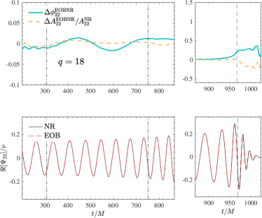
Figure 12: Phasing comparison for $q=18$: comparison between TEOBiResumMultipoles and the corresponding NR waveform data obtained with the BAM code. The two waveforms are highly compatible even if this dataset was not used to inform $a_{6}^{c}(\nu)$. Note the effect of the (rather small) eccentricity that shows up as an oscillation in the phase difference (top panel).

VII.2 Unfaithfulness

The second comparison we discuss is that of the EOB/NR unfaithfulness. Given $h_{i}$ a waveform and $\tilde{h}_{i}(f)$ its Fourier transform, we define the following weighted scalar product between two waveforms

$$\left\langle h_{1}|h_{2}\right\rangle=4\,\operatorname{Re}\int^{f_{h}}_{f_{l}}\frac{\tilde{h}_{1}^{*}(f)\;\tilde{h}_{2}(f)}{S_{n}(f)}\;df,$$ (93)

where $S_{n}(f)$ is the power spectral density (PSD) of the detector. The unfaithfulness $\bar{{F}}$ can then be defined via the inner product between normalised ($\hat{h}=h/\sqrt{\langle h|h\rangle}$) waveforms maximised over time and phase shifts

$$\bar{{F}}(h_{1},h_{2}) =1-F=1-\max\limits_{t_{0},\phi_{0}}\,\langle\hat{h}_{1}|\hat{h}_{2}\rangle.$$ (94)

Note that the maximization over time and phase shifts has no physical significance, corresponding to a change in the merger time and initial phase of the binary. In our analysis, we use the zero-detuned high-power (zdethp) power spectrum Abbott et al. (2018b); Shoemaker as a representative PSD for aLIGO at design sensitivity. As the NR waveforms are of finite length, we use a lower cutoff frequency of $f_{l}={\rm{min}}\,(20,f_{\rm{NR}})$ Hz and an upper cut-off frequency of $f_{h}=2048$Hz.

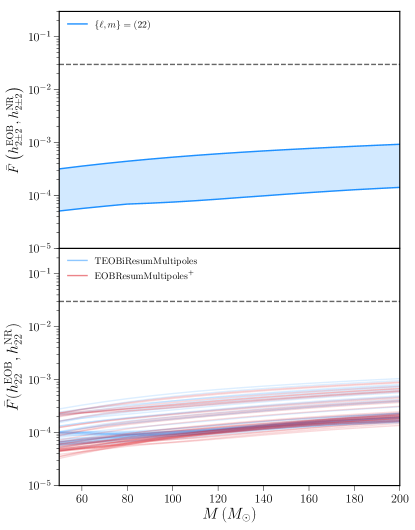
Figure 13: Top panel: Unfaithfulness between SXS simulations and TEOBiResumMultipoles for mass ratios $q\in[2,10]$. Note that we use the zero-detuned high power Advanced LIGO design sensitivity PSD and assume a face-on configuration. We restrict the analysis to the dominant $(2,2)$ mode, demonstrating the baseline performance of the model when neglecting higher order modes. The model is everywhere below $10^{-3}$ for $M\lesssim 200M_{\odot}$. Bottom panel: comparison between TEOBiResumMultipoles and EOBResumMultipoles⁺. The two models, that are relying on different determinations of $a_{6}^{c}(\nu)$ induced by different resummation choices in the radiation reaction, are practically equivalent.

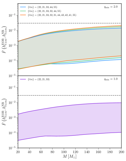
Figure 14: Unfaithfulness between TEOBiResumMultipoles and SXS simulations for mass ratios using the zero-detuned high power Advanced LIGO design sensitivity PSD. We show the minimum and maximum unfaithfulness over all angles $(\theta,\varphi)$, demonstrating that the worst case performance is always below $3$% for binaries with a total mass $M\lesssim 200M_{\odot}$. Even though TEOBiResumMultipoles neglects mode-mixing, we do not find a significant degradation in performance when considering $(3,2)$ mode (red curves) or all modes up to $\ell=4$ and the $(5,5)$ mode (green curve). In the top panel, we restrict the analysis to $q\geq 2$ due to the issues highlighted in the text. In the bottom panel, where we neglect the $(4,4)$ mode, we find excellent agreement with NR down to $q=1$.

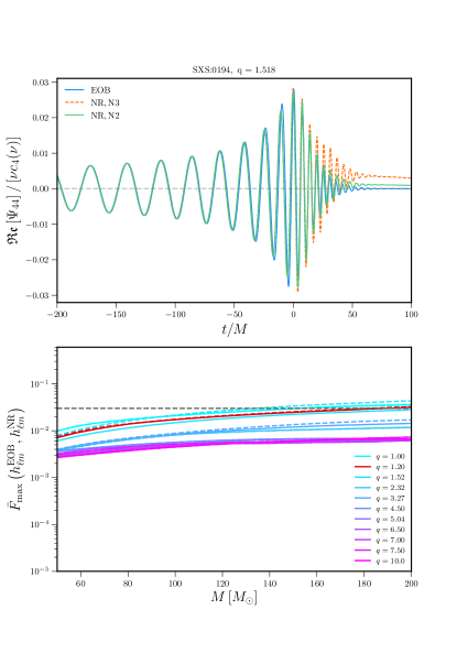
Figure 15: Top panel: systematic effects show up in the $\ell=m=4$ mode of SXS:BBH:0194 when extrapolated with the standard choice $N=3$. Bottom panel: Unfaithfulness against selected SXS simulations using $N=3$ extrapolated waveforms (dashed) and $N=2$ extrapolated waveforms (solid). As the mass ratio increases, the difference between the two extrapolation orders becomes negligible.

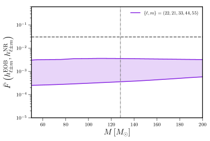
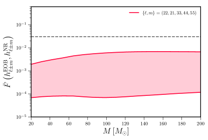
Figure 16: Minimum and maximum unfaithfulness for TEOBiResumMultipoles model against a BAM $q=18$ waveform Husa et al. (2016) (top panel) and an SXS $q=6$ simulation (bottom panel). In the top panel, the dot-dashed line shows the minimum mass for which the entire NR waveform is in band. The EOB/NR performance for $q=6$ is comparable to (though slightly better than) SEOBNRv4HM, for the same SXS dataset, as deducible by comparison with Fig. 16 of Ref. Cotesta et al. (2018).

In Fig. 11 we illustrate the performance gain obtained by TEOBiResumMultipoles with higher modes included when comparing to SXS:BBH:0303, a high mass ratio $q=10$ binary. As one may expect, using only the $(2,2)$-mode in constructing the strain results in an unfaithfulness against the NR waveforms that is degraded by at least two orders of magnitude. This can be seen in the right panel of Fig. 11. The baseline performance of the dominant $(2,2)$ mode is everywhere below $10^{-3}$ for $M\lesssim 200M_{\odot}$, as one sees in the top-panel of Fig. 13. The same figure, in the bottom panel, illustrates the excellent consistency between TEOBiResumMultipoles and EOBResumMultipoles⁺, although the two models differ both in the description of the radiation reaction and in the determination of $a_{6}^{c}(\nu)$. When considering higher modes, we have verified that, for $\ell\geq 3$, the mode-by-mode EOB/NR unfaithfulness is slightly, but nonnegligibly, smaller for TEOBiResumMultipoles than for EOBResumMultipoles⁺, so that we will not discuss this latter any further. Including several higher order modes in TEOBiResumMultipoles, we found that the EOB/NR unfaithfulness is everywhere below $3\%$ for binaries up to $M<200M_{\odot}$, as demonstrated in Fig. 14. Note however that we focus here on $q\in[2,10]$. The range $1\leq q\leq 2$ has some issues that we discuss below. However, when neglecting the $(4,4)$ mode, the model performance is in excellent agreement with NR down to $q=1$, as seen in the bottom panel of Fig. 14. When taking into account the $(3,2)$ mode, the most prominent mode affected by mode-mixing Berti and Klein (2014), we find that the performance of the model only slightly degrades across the whole parameter space and the unfaithfulness robustly remains below $3$% for binaries up to $\lesssim 200M_{\odot}$.

We investigated the origin of the behavior of $\bar{F}$ for large masses. We discovered that it does not come from inaccuracies in the analytical description of the ringdown (e.g. the lack of mode mixing effects) but rather from the amplification of some NR numerical noise present in the ringdown due to the extrapolation of the waveforms. We recall in this respect, that in the SpEC code the waveforms are extracted at finite radius and then extrapolated to infinite distance using polynomials in the inverse power of the extraction radius. The highest power of this polynomial is labeled as $N$. In the SXS catalog, data extrapolated with different values of $N$ are provided. It is well known that non-optimal values of $N$ may introduce unphysical features and thus such extrapolation process can be quite delicate Boyle and Mroue (2009). Investigating the various datasets present in the SXS catalog for each configuration, we have found that such amplification of the late-time NR noise shows up only for some nearly-equal-mass configuration when the (standard) extrapolation order $N=3$ is used. We recall that the SXS collaboration advises catalog users to employ low values of $N$ if one is interested in studying the ringdown and large values of $N$ if one is more focused on the inspiral. Here, we use the $N=3$ extrapolation order as a reasonable compromise for the whole waveform, although, as mentioned above, we use the $N=2$ extrapolation order to obtain the post-merger fits as the NR data is typically cleaner. This phenomenon is illustrated in the top panel of Fig. 15, for SXS:BBH:0194. One sees that the $N=3$ extrapolation introduces an unphysical offset during the ringdown that is reduced, though not completely eliminated, when using an $N=2$ extrapolation order. Such systematic effect also shows up in the unfaithfulness, which is shown in the bottom panel of the Fig. 15 for several mass ratios. The dashed lines correspond to using $N=3$ data, while the solid lines are for the $N=2$ data. It is also interesting to note that the differences between extrapolation orders becomes progressively negligible as the mass ratio increases. In Fig. 16, we compare TEOBiResumMultipoles against a non-spinning $q=18$ BAM simulation, finding excellent agreement against the model. In the bottom panel of the same figure we also show the same comparison for the $q=6$ SXS dataset. An analogous comparison is also displayed in Fig. 16 of Cotesta et al. (2018) for the SEOBNRv4HM model, that incorporates the same number of subdominant modes considered in this figure. We find that the performance of TEOBiResumMultipoles on this particular SXS dataset is comparable to that of SEOBNRv4HM, though slightly better especially for low masses. To ease this comparison, in this case we used $20M_{\odot}$ as lower-mass boundary. Our analysis illustrates that the EOB/NR $\bar{F}$ comparison may be slightly misleading, and TEOBiResumMultipoles delivers a faithful representation of the multipolar waveform also for nearly-equal-mass binaries.

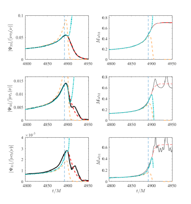
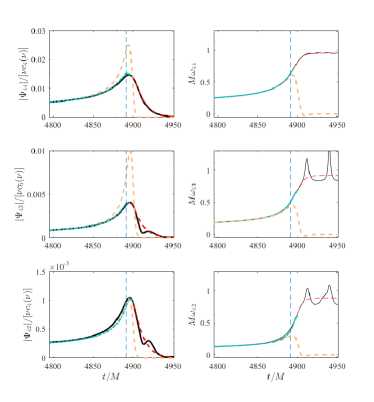
Figure 17: Mass ratio $q=6$, SXS:BBH:0166. Frequency and amplitude comparison, $\ell=3$ and $\ell=4$ multipoles. Black line: NR data. Orange (dashed) lines: bare EOB waveform. Blue lines: NQC-modified waveform; red line: postmerger-ringdown part. The vertical, dashed, line marks the merger location. Note that mode-mixing is not incorporated in the analytical ringdown description.

Figure 18: Mass ratio $q=6$, SXS:BBH:0166. EOB/NR comparison for $(4,1)$ mode (left) and $(5,5)$ mode (right). Although the $(4,1)$ numerical frequency is rather noisy, it shows a good qualitative agreement with the analytical EOB prediction. In addition, the EOB and NR $(5,5)$ frequencies are remarkably close during the full transition from inspiral to plunge, merger and ringdown. For both modes, the NQC-corrected analytical amplitude close to merger tends to be larger then, though consistent with, the NR one.

VIII Conclusions

We have presented TEOBiResumMultipoles, a new, NR-informed, EOB model for nonspinning black hole binaries that incorporates higher multipolar waveform modes. The multipoles are complete through merger and ringdown up to $\ell=m=5$ included. The additional waveform modes up to $\ell=8$ (including $\ell=5$, $|m|<5$) are also included but they rely on the, purely analytical, EOB-resummed waveform. In practical terms, this means that the corresponding EOB GW frequency $\omega_{\ell m}^{\rm EOB}$ smoothly goes to zero after merger and does not saturate to the plateau corresponding to the QNM excitation. Up to the merger point, it generally delivers an excellent approximation to the multipolar NR frequency $\omega_{{\ell m}}^{\rm NR}$. Our main findings can be summarized as follows:

• At a purely analytical level, the major novelty introduced here is that the $\nu$-dependent terms entering the factorized waveform amplitudes $\rho_{\ell m}$ are hybridized with test-particle information up to (relative) 6PN order (i.e. each $\rho_{\ell m}$ is given by a 6-th order polynomial in some squared velocity variable). As a second step, such polynomials are additionally resummed using Padé approximants consistent with test-particle limit results Messina et al. (2018). This approach improves the robustness of the waveform amplitude across the parameter space, improves the stability of the NQC corrections and bridges the gap, at least for what concerns the waveform and radiation reaction effects, with the test-particle limit Nagar and Shah (2016); Messina et al. (2018).

• Each multipolar mode up to $\ell=m=5$ is completed through merger and ringdown by means of the NQC correction factor and NR-informed post-merger behavior. The transition between the inspiral-merger phase and the post-merger ringdown can be easily, and naturally, performed just after the peak of each multipole, at the NQC determination point.

• To have each separate EOB waveform multipole (both the amplitude and phase) correct around its own amplitude peak requires five functions of $\nu$ that are determined using NR simulations: $\left\{\Delta t_{\ell m}^{\rm NR},A_{\ell m}^{\rm NQC},\dot{A}_{\ell m}^{\rm NQC},\omega_{\ell m}^{\rm NQC},\dot{\omega}_{\ell m}^{\rm NQC}\right\}$. This allows us to properly determine the NQC correction factor multipole by multipole. This is a crucial piece of information that must be added to the purely analytical description of each waveform multipole in order to correctly represent the very latest stages of the evolution, $\sim 50M$ before the peak. It is remarkable that such a straightforward procedure is so efficient in improving, multipole by multipole, the circularized EOB waveform. This is also the case for the $m=1$ mode, where the impact of the radial-momentum dependent terms can be particularly large. Note, however, that this approach only works in conjunction with the structure of the Newtonian (multipolar) prefactors, that should be effectively modified by relaxing, in a specific multipole dependent way, Newton’s Kepler’s constraint during the plunge. This allows one to ease the action of the NQC factors.

• In order to gauge some of the analytical uncertainty associated to the choices made in constructing a NR-informed EOB model, we have contrasted the effect of two different choices of radiation reaction. This corresponds to two different and independent determinations of $a_{6}^{c}(\nu)$ obtained through an EOB/NR phasing comparison. Eventually, we conclude that the choice made for TEOBiResumMultipoles, that relies on Padé resummed waveform amplitudes, is more accurate and robust, especially in view of its use in a forthcoming spin-aligned multipolar waveform model.

• We have performed an extensive investigation of the EOB/NR unfaithfulness varying both the mass ratio and the viewing direction of the waveform. The global multipolar model was found to yield an unfaithfulness always $<3$% for binaries of $50\leq M\leq 200M_{\odot}$. We could clearly probe that such degradation of the EOB/NR performance, that occurs for large masses and only for some specific region of the parameter space with $1\lesssim q\lesssim 2$, is mainly due to uncertainties in the NR higher modes that may be amplified due to, for example, the extrapolation procedures. By contrast, one has also to remark that $\bar{F}$ comfortably remains below (or around) $1\%$ up to total mass of the order of $100M_{\odot}$.

• For the first time, we have provided an EOB-based description of the $(3,2)$ and $(4,3)$ waveform modes through merger and ringdown, although we did so neglecting mode mixing effects. We found that such approximation does not seem to especially degrade the performance of the model.

The TEOBiResumMultipoles model presented here will be made publicly available as a stand-alone $C$-implementation (notably complemented by the fast post-adiabatic approximation for the inspiral Nagar and Rettegno (2019)) as well as within the LIGO LALSuite library.

Appendix A Detailed amplitude and frequency EOB/NR comparisons for higher modes

This Appendix collects some complementary information behind the global view plot of Fig. 9. Figures 17 and 18 show EOB/NR amplitude amplitude frequency comparisons for the illustrative case SXS:BBH:0166, with $q=6$ for the $\ell=3$, $\ell=4$ and $\ell=m=5$ modes. As above, the dashed vertical line identifies the merger point. In general, the bare EOB frequency (orange, dashed line) gives a reliable representation of the NR one essentially up to merger for the $\ell=m$ modes. Similarly, the NQC correction factor is able to efficiently bridge the gap with the postpeak (ringdown) part for all multipoles, even the $(3,2)$ and $(4,3)$, although our model just averages on the postpeak behavior due to mode-mixing effects. The proof of the robustness of the ringdown-matching procedure is evident also in an (essentially) irrelevant mode like the $(4,1)$, where the analytic model is able to accurately interpolate in a region where NR data are rather noisy.

Appendix B Interpolating fit for the NQC extraction point

This Appendix lists the fits of waveform amplitude and frequency values extracted at the special NQC point on the NR time axis. These fits are then used to determine the parameters $(a_{1}^{\ell m},a_{2}^{\ell m},b_{1}^{\ell m},b_{2}^{\ell m})$ entering the multipolar NQC correction factors of Eq. (32). We focus here on the fits for all modes with the exception of the $(2,1)$ one that is separately treated in Sec. B.1 below due to the special behavior in the test-particle limit. For each mode, the NQC point is located $2M$ on the right of the peak location. We fit the NR waveform data (amplitude, frequency and first time derivatives) extracted there with a factorized template of the form

$$Y^{\rm NQC}_{\ell m}=Y^{0}_{\ell m}\;\hat{\hat{Y}}^{\rm NQC}_{\ell m},$$ (95)

where $Y^{0}_{\ell m}$ refers to the test-particle limit value and $\hat{\hat{Y}}^{\rm NQC}_{\ell m}$ captures the remaining $\nu$-dependence. The latter is modeled with a rational function or polynomial up to second order in $\nu$, in both denominator and numerator. The reader should note that the amplitude is not fitted directly, but rather we use the quantity $\hat{A}^{{\rm NQC}}_{\ell m}\equiv A^{\rm NQC}_{\ell m}/|c_{\ell+\epsilon}(\nu)|$. The parameter of the fits are reported in the Table 7.

B.1 $(\ell,m)=(2,1)$ mode

The values of frequency and amplitude at the $(2,1)$ NQC extraction point $t_{21}^{\rm NQC}$ are directly fitted with linear and quadratic polynomials in $\nu$, and the factorization of the test-particle values is omitted. The reason for doing so is the peculiar (well-known) behavior of the frequency in the test-particle limit, that is illustrated in Fig. 19. One sees that the frequency $M\omega_{21}$ starts to oscillate after the peak of the $(2,1)$ mode. These oscillations are due to the interference of negative and positive QNMs Nagar et al. (2007); Damour and Nagar (2007); Bernuzzi and Nagar (2010). Because this phenomenon shows up at $t^{\rm NQC}_{21}$, factoring out the test-particle behavior is no longer beneficiary to the fit quality, at least with the sample of NR data currently at our disposal. The $(2,1)$ fits are listed in the second row of Table 7.

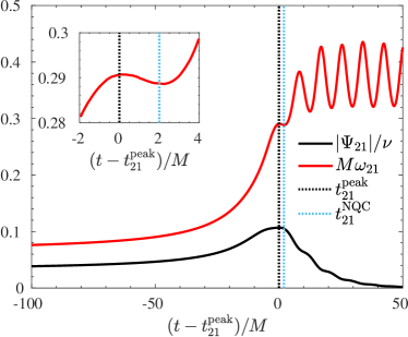
Figure 19: The amplitude $|\Psi_{21}|/\nu$ and frequency $M\omega_{21}$ of the $(2,1)$ mode in the extreme-mass-ratio limit for a BBH coalescence in the large mass ratio limit. The waveform is obtained using a Regge-Wheeler-Zerilli perturbative approach, where a test-mass inspirals and plunges over a Schwarzschild black hole. The frequency $M\omega_{21}$(red) starts to oscillate after the peak because of the interference between negative and positive frequency QNMs Nagar et al. (2007); Damour and Nagar (2007); Bernuzzi and Nagar (2010). The inset zooms on $M\omega_{21}$ at the peak of the $(2,1)$ mode.

Table 7: The fits of the NQC functioning points $\{\hat{A}^{{\rm NQC}}_{\ell m},\dot{A}^{{\rm NQC}}_{\ell m}/\nu,\omega^{\rm NQC}_{\ell m},\dot{\omega}^{\rm NQC}_{\ell m}\}$. The fits are given explicitly. The fits are done after the factorization defined in eq. (95). For all multipoles the factorization of the test-particle limit $Y^{0}_{\ell m}$ is highlighted explicitly in the third and fifth column of the table. The exception to this is the $(2,1)$ mode for which the test-particle behavior has not been factorized (see Sec. B.1). $\hat{\hat{Y}}^{\rm NQC}_{\ell m}$ is fitted for all multipoles with at most quadratic polynomials or rational functions in $\nu$. The reader should note that $A^{{\rm NQC}}_{\ell m}=|c_{\ell+\epsilon}(\nu)|\hat{A}^{{\rm NQC}}_{\ell m}$.

		$\hat{A}^{{\rm NQC}}_{\ell m}$		$\omega^{\rm NQC}_{\ell m}$
2	2	$0.294773$	$\left(1-0.051898\nu+1.5886\nu^{2}\right)$	$0.285588$	$\left(1+0.92487\nu+1.7206\nu^{2}\right)$
2	1	$0.097671-0.0014424\nu$		$0.29622+0.048182\nu+0.37472\nu^{2}$
3	3	$0.0512928$	$\left(1+0.09537\nu+3.7217\nu^{2}\right)$	$0.476647$	$\left(1+1.1008\nu+2.84\nu^{2}\right)$
3	2	$0.0178914$	$\left(\frac{1-6.1472\nu+11.435\nu^{2}}{1-3.6362\nu}\right)$	$0.482635$	$\left(\frac{1-9.1403\nu+21.399\nu^{2}}{1-8.8647\nu+20.185\nu^{2}}\right)$
3	1	$0.00520201$	$\left(1-4.9441\nu+8.9339\nu^{2}\right)$	$0.485186$	$\left(1-0.4421\nu-6.8184\nu^{2}\right)$
4	4	$0.0144330$	$\left(\frac{1-3.7335\nu-0.2895\nu^{2}}{1-3.7298\nu}\right)$	$0.665507$	$\left(1+0.95802\nu\right)$
4	3	$0.00487784$	$\left(\frac{1-5.7951\nu+12.833\nu^{2}}{1-3.2681\nu}\right)$	$0.673274$	$\left(\frac{1-9.2007\nu+22.161\nu^{2}}{1-9.026\nu+21.238\nu^{2}}\right)$
4	2	$0.00161809$	$\left(1-4.6975\nu+7.3437\nu^{2}\right)$	$0.663076$	$\left(1-0.086381\nu-8.5978\nu^{2}\right)$
4	1	$0.00043987$	$\left(\frac{1-8.4975\nu+27.31\nu^{2}}{1-1.2002\nu}\right)$	$0.735051$	$\left(\frac{1-8.3628\nu+20.529\nu^{2}}{1-7.4883\nu+18.695\nu^{2}}\right)$
5	5	$0.00516272$	$\left(1-0.38892\nu+6.7413\nu^{2}\right)$	$0.855016$	$\left(\frac{1-2.8461\nu-3.7163\nu^{2}}{1-3.8378\nu}\right)$
		$\dot{A}^{{\rm NQC}}_{\ell m}/\nu$		$\dot{\omega}^{\rm NQC}_{\ell m}$
2	2	$-0.00119366$	$\left(1+3.0125\nu-2.1792\nu^{2}\right)$	$0.00628027$	$\left(1+2.5374\nu+3.9341\nu^{2}\right)$
2	1	$\left(-0.0011119+0.0042824\nu\right)/\left(1-3.0565\nu\right)$		$0.0020157+0.049725\nu$
3	3	$-0.00039568$	$\left(1+1.0985\nu-13.458\nu^{2}\right)$	$0.0110394$	$\left(1+2.1358\nu+4.1544\nu^{2}\right)$
3	2	$-0.00026840$	$\left(\frac{1-8.4869\nu+18.736\nu^{2}}{1-5.7457\nu+7.9581\nu^{2}}\right)$	$0.0141756$	$\left(\frac{1-10.831\nu+37.969\nu^{2}}{1-12.954\nu+51.155\nu^{2}}\right)$
3	1	$-0.00043382$	$\left(\frac{1-9.0479\nu+23.054\nu^{2}}{1+88.626\nu^{2}}\right)$	$0.0673118$	$\left(\frac{1+13.318\nu}{1+70.552\nu}\right)$
4	4	$-0.00015129$	$\left(1-2.206\nu+2.0191\nu^{2}\right)$	$0.0147878$	$\left(\frac{1-3.4516\nu+4.8703\nu^{2}}{1-5.7616\nu+11.286\nu^{2}}\right)$
4	3	$-0.00008468$	$\left(1-4.1848\nu+4.2192\nu^{2}\right)$	$0.0172836$	$\left(\frac{1-19.234\nu+105.04\nu^{2}}{1-19.837\nu+107.76\nu^{2}}\right)$
4	2	$-0.00004223$	$\left(\frac{1-5.1172\nu+5.4408\nu^{2}}{+6.1593\nu}\right)$	$0.0213781$	$\left(\frac{1-6.2629\nu+10.1\nu^{2}}{1-8.4232\nu+21.204\nu^{2}}\right)$
4	1	$-0.00001827$	$\left(1-2.8242\nu-3.1871\nu^{2}\right)$	$0.0739078$	$\left(1+0.99186\nu-19.435\nu^{2}\right)$
5	5	$-0.00006580$	$\left(1-1.8592\nu\right)$	$0.0178326$	$\left(1+2.4606\nu\right)$

References

- Aasi et al. (2015) J. Aasi et al. (LIGO Scientific), Class. Quant. Grav. 32, 074001 (2015), arXiv:1411.4547 [gr-qc] .
- Acernese et al. (2015) F. Acernese et al. (VIRGO), Class. Quant. Grav. 32, 024001 (2015), arXiv:1408.3978 [gr-qc] .
- Abbott et al. (2016a) B. P. Abbott et al. (Virgo, LIGO Scientific), Phys. Rev. Lett. 116, 061102 (2016a), arXiv:1602.03837 [gr-qc] .
- Abbott et al. (2016b) B. P. Abbott et al. (Virgo, LIGO Scientific), Phys. Rev. Lett. 116, 241103 (2016b), arXiv:1606.04855 [gr-qc] .
- Abbott et al. (2017a) B. P. Abbott et al. (VIRGO, LIGO Scientific), Phys. Rev. Lett. 118, 221101 (2017a), arXiv:1706.01812 [gr-qc] .
- Abbott et al. (2017b) B. P. Abbott et al. (Virgo, LIGO Scientific), Astrophys. J. 851, L35 (2017b), arXiv:1711.05578 [astro-ph.HE] .
- Abbott et al. (2017c) B. P. Abbott et al. (Virgo, LIGO Scientific), Phys. Rev. Lett. 119, 141101 (2017c), arXiv:1709.09660 [gr-qc] .
- Abbott et al. (2018a) B. P. Abbott et al. (LIGO Scientific, Virgo), (2018a), arXiv:1811.12907 [astro-ph.HE] .
- Abbott et al. (2017d) B. P. Abbott et al. (Virgo, LIGO Scientific), Phys. Rev. Lett. 119, 161101 (2017d), arXiv:1710.05832 [gr-qc] .
- Abbott et al. (2017e) B. P. Abbott et al. (Virgo, LIGO Scientific), Class. Quant. Grav. 34, 104002 (2017e), arXiv:1611.07531 [gr-qc] .
- O’Shaughnessy et al. (2014) R. O’Shaughnessy, B. Farr, E. Ochsner, H.-S. Cho, V. Raymond, C. Kim, and C.-H. Lee, Phys. Rev. D89, 102005 (2014), arXiv:1403.0544 [gr-qc] .
- Varma and Ajith (2017) V. Varma and P. Ajith, Phys. Rev. D96, 124024 (2017), arXiv:1612.05608 [gr-qc] .
- Capano et al. (2014) C. Capano, Y. Pan, and A. Buonanno, Phys. Rev. D89, 102003 (2014), arXiv:1311.1286 [gr-qc] .
- Calderón Bustillo et al. (2017) J. Calderón Bustillo, P. Laguna, and D. Shoemaker, Phys. Rev. D95, 104038 (2017), arXiv:1612.02340 [gr-qc] .
- Harry et al. (2018) I. Harry, J. Calderón Bustillo, and A. Nitz, Phys. Rev. D97, 023004 (2018), arXiv:1709.09181 [gr-qc] .
- Dreyer et al. (2004) O. Dreyer, B. J. Kelly, B. Krishnan, L. S. Finn, D. Garrison, and R. Lopez-Aleman, Class. Quant. Grav. 21, 787 (2004), arXiv:gr-qc/0309007 [gr-qc] .
- Berti et al. (2006) E. Berti, V. Cardoso, and C. M. Will, Phys. Rev. D73, 064030 (2006), arXiv:gr-qc/0512160 .
- Kamaretsos et al. (2012a) I. Kamaretsos, M. Hannam, S. Husa, and B. S. Sathyaprakash, Phys. Rev. D85, 024018 (2012a), arXiv:1107.0854 [gr-qc] .
- Gossan et al. (2012) S. Gossan, J. Veitch, and B. S. Sathyaprakash, Phys. Rev. D85, 124056 (2012), arXiv:1111.5819 [gr-qc] .
- Kamaretsos et al. (2012b) I. Kamaretsos, M. Hannam, and B. Sathyaprakash, Phys.Rev.Lett. 109, 141102 (2012b), arXiv:1207.0399 [gr-qc] .
- Meidam et al. (2014) J. Meidam, M. Agathos, C. Van Den Broeck, J. Veitch, and B. S. Sathyaprakash, Phys. Rev. D90, 064009 (2014), arXiv:1406.3201 [gr-qc] .
- London et al. (2014) L. London, D. Shoemaker, and J. Healy, Phys. Rev. D90, 124032 (2014), [Erratum: Phys. Rev.D94,no.6,069902(2016)], arXiv:1404.3197 [gr-qc] .
- Berti et al. (2016) E. Berti, A. Sesana, E. Barausse, V. Cardoso, and K. Belczynski, Phys. Rev. Lett. 117, 101102 (2016), arXiv:1605.09286 [gr-qc] .
- Cardoso and Gualtieri (2016) V. Cardoso and L. Gualtieri, Class. Quant. Grav. 33, 174001 (2016), arXiv:1607.03133 [gr-qc] .
- Yang et al. (2017) H. Yang, K. Yagi, J. Blackman, L. Lehner, V. Paschalidis, F. Pretorius, and N. Yunes, Phys. Rev. Lett. 118, 161101 (2017), arXiv:1701.05808 [gr-qc] .
- Brito et al. (2018) R. Brito, A. Buonanno, and V. Raymond, Phys. Rev. D98, 084038 (2018), arXiv:1805.00293 [gr-qc] .
- Carullo et al. (2018) G. Carullo et al., Phys. Rev. D98, 104020 (2018), arXiv:1805.04760 [gr-qc] .
- Pan et al. (2011) Y. Pan, A. Buonanno, M. Boyle, L. T. Buchman, L. E. Kidder, et al., Phys.Rev. D84, 124052 (2011), arXiv:1106.1021 [gr-qc] .
- Damour et al. (2013) T. Damour, A. Nagar, and S. Bernuzzi, Phys.Rev. D87, 084035 (2013), arXiv:1212.4357 [gr-qc] .
- Cotesta et al. (2018) R. Cotesta, A. Buonanno, A. Bohé, A. Taracchini, I. Hinder, and S. Ossokine, Phys. Rev. D98, 084028 (2018), arXiv:1803.10701 [gr-qc] .
- Mehta et al. (2017) A. K. Mehta, C. K. Mishra, V. Varma, and P. Ajith, Phys. Rev. D96, 124010 (2017), arXiv:1708.03501 [gr-qc] .
- London et al. (2018) L. London, S. Khan, E. Fauchon-Jones, X. J. Forteza, M. Hannam, S. Husa, C. Kalaghatgi, F. Ohme, and F. Pannarale, Phys. Rev. Lett. 120, 161102 (2018), arXiv:1708.00404 [gr-qc] .
- Nagar et al. (2018) A. Nagar et al., Phys. Rev. D98, 104052 (2018), arXiv:1806.01772 [gr-qc] .
- Damour and Nagar (2014a) T. Damour and A. Nagar, Phys.Rev. D90, 024054 (2014a), arXiv:1406.0401 [gr-qc] .
- Del Pozzo and Nagar (2017) W. Del Pozzo and A. Nagar, Phys. Rev. D95, 124034 (2017), arXiv:1606.03952 [gr-qc] .
- Harms et al. (2014) E. Harms, S. Bernuzzi, A. Nagar, and A. Zenginoglu, Class.Quant.Grav. 31, 245004 (2014), arXiv:1406.5983 [gr-qc] .
- Borhanian et al. (2019) S. Borhanian, K. G. Arun, H. P. Pfeiffer, and B. S. Sathyaprakash, (2019), arXiv:1901.08516 [gr-qc] .
- Damour et al. (2000) T. Damour, P. Jaranowski, and G. Schaefer, Phys. Rev. D62, 084011 (2000), arXiv:gr-qc/0005034 [gr-qc] .
- Damour and Nagar (2014b) T. Damour and A. Nagar, Phys.Rev. D90, 044018 (2014b), arXiv:1406.6913 [gr-qc] .
- Bini and Damour (2012) D. Bini and T. Damour, Phys.Rev. D86, 124012 (2012), arXiv:1210.2834 [gr-qc] .
- Nagar et al. (2016) A. Nagar, T. Damour, C. Reisswig, and D. Pollney, Phys. Rev. D93, 044046 (2016), arXiv:1506.08457 [gr-qc] .
- Damour et al. (2009) T. Damour, B. R. Iyer, and A. Nagar, Phys. Rev. D79, 064004 (2009), arXiv:0811.2069 [gr-qc] .
- Bernuzzi et al. (2012) S. Bernuzzi, A. Nagar, and A. Zenginoglu, Phys.Rev. D86, 104038 (2012), arXiv:1207.0769 [gr-qc] .
- Nagar and Akcay (2012) A. Nagar and S. Akcay, Phys.Rev. D85, 044025 (2012), arXiv:1112.2840 [gr-qc] .
- Damour (2010) T. Damour, Phys. Rev. D81, 024017 (2010), arXiv:0910.5533 [gr-qc] .
- Blanchet et al. (2010) L. Blanchet, S. L. Detweiler, A. Le Tiec, and B. F. Whiting, Phys.Rev. D81, 084033 (2010), arXiv:1002.0726 [gr-qc] .
- Barausse et al. (2012) E. Barausse, A. Buonanno, and A. Le Tiec, Phys.Rev. D85, 064010 (2012), arXiv:1111.5610 [gr-qc] .
- Bini and Damour (2013) D. Bini and T. Damour, Phys.Rev. D87, 121501 (2013), arXiv:1305.4884 [gr-qc] .
- Kavanagh et al. (2015) C. Kavanagh, A. C. Ottewill, and B. Wardell, Phys. Rev. D92, 084025 (2015), arXiv:1503.02334 [gr-qc] .
- Damour and Nagar (2007) T. Damour and A. Nagar, Phys. Rev. D76, 064028 (2007), arXiv:0705.2519 [gr-qc] .
- Damour and Gopakumar (2006) T. Damour and A. Gopakumar, Phys. Rev. D73, 124006 (2006), arXiv:gr-qc/0602117 .
- Nagar et al. (2019) A. Nagar, F. Messina, P. Rettegno, D. Bini, T. Damour, A. Geralico, S. Akcay, and S. Bernuzzi, Phys. Rev. D99, 044007 (2019), arXiv:1812.07923 [gr-qc] .
- Akcay et al. (2019) S. Akcay, S. Bernuzzi, F. Messina, A. Nagar, N. Ortiz, and P. Rettegno, Phys. Rev. D99, 044051 (2019), arXiv:1812.02744 [gr-qc] .
- Damour and Nagar (2009) T. Damour and A. Nagar, Phys. Rev. D79, 081503 (2009), arXiv:0902.0136 [gr-qc] .
- Fujita (2015) R. Fujita, PTEP 2015, 033E01 (2015), arXiv:1412.5689 [gr-qc] .
- Fujita (2012) R. Fujita, Prog.Theor.Phys. 128, 971 (2012), arXiv:1211.5535 [gr-qc] .
- Nagar and Shah (2016) A. Nagar and A. Shah, Phys. Rev. D94, 104017 (2016), arXiv:1606.00207 [gr-qc] .
- Messina et al. (2018) F. Messina, A. Maldarella, and A. Nagar, Phys. Rev. D97, 084016 (2018), arXiv:1801.02366 [gr-qc] .
- Nagar et al. (2017) A. Nagar, G. Riemenschneider, and G. Pratten, Phys. Rev. D96, 084045 (2017), arXiv:1703.06814 [gr-qc] .
- Bini and Damour (2014) D. Bini and T. Damour, Phys.Rev. D89, 064063 (2014), arXiv:1312.2503 [gr-qc] .
- Bohé et al. (2017) A. Bohé et al., Phys. Rev. D95, 044028 (2017), arXiv:1611.03703 [gr-qc] .
- Jiménez-Forteza et al. (2017) X. Jiménez-Forteza, D. Keitel, S. Husa, M. Hannam, S. Khan, and M. Pürrer, Phys. Rev. D95, 064024 (2017), arXiv:1611.00332 [gr-qc] .
- Mroue et al. (2013) A. H. Mroue, M. A. Scheel, B. Szilagyi, H. P. Pfeiffer, M. Boyle, et al., Phys.Rev.Lett. 111, 241104 (2013), arXiv:1304.6077 [gr-qc] .
- Chu et al. (2016) T. Chu, H. Fong, P. Kumar, H. P. Pfeiffer, M. Boyle, D. A. Hemberger, L. E. Kidder, M. A. Scheel, and B. Szilagyi, Class. Quant. Grav. 33, 165001 (2016), arXiv:1512.06800 [gr-qc] .
- Blackman et al. (2015) J. Blackman, S. E. Field, C. R. Galley, B. Szilágyi, M. A. Scheel, M. Tiglio, and D. A. Hemberger, Phys. Rev. Lett. 115, 121102 (2015), arXiv:1502.07758 [gr-qc] .
- (66) https://data.black-holes.org/waveforms/index.html, sXS Gravitational Waveform Database.
- Nagar and Rezzolla (2005) A. Nagar and L. Rezzolla, Class. Quant. Grav. 22, R167 (2005), arXiv:gr-qc/0502064 .
- Bernuzzi and Nagar (2010) S. Bernuzzi and A. Nagar, Phys. Rev. D81, 084056 (2010), arXiv:1003.0597 [gr-qc] .
- Damour et al. (2012) T. Damour, A. Nagar, D. Pollney, and C. Reisswig, Phys.Rev.Lett. 108, 131101 (2012), arXiv:1110.2938 [gr-qc] .
- Ossokine et al. (2018) S. Ossokine, T. Dietrich, E. Foley, R. Katebi, and G. Lovelace, Phys. Rev. D98, 104057 (2018), arXiv:1712.06533 [gr-qc] .
- LIGO Scientific Collaboration (2018) LIGO Scientific Collaboration, “LIGO Algorithm Library - LALSuite,” free software (GPL) (2018).
- (72) R. Gamba, https://bitbucket.org/RoxGamba/seobnrv4_hacked_ej/src/master/.
- Damour and Nagar (2008) T. Damour and A. Nagar, Phys. Rev. D77, 024043 (2008), arXiv:0711.2628 [gr-qc] .
- Abbott et al. (2018b) B. P. Abbott et al. (VIRGO, KAGRA, LIGO Scientific), Living Rev. Rel. 21, 3 (2018b), [Living Rev. Rel.19,1(2016)], arXiv:1304.0670 [gr-qc] .
- (75) D. Shoemaker, https://dcc.ligo.org/cgi-bin/DocDB/ShowDocument?docid=2974 .
- Husa et al. (2016) S. Husa, S. Khan, M. Hannam, M. Pürrer, F. Ohme, X. Jiménez Forteza, and A. Bohé, Phys. Rev. D93, 044006 (2016), arXiv:1508.07250 [gr-qc] .
- Berti and Klein (2014) E. Berti and A. Klein, Phys. Rev. D90, 064012 (2014), arXiv:1408.1860 [gr-qc] .
- Boyle and Mroue (2009) M. Boyle and A. H. Mroue, Phys. Rev. D80, 124045 (2009), arXiv:0905.3177 [gr-qc] .
- Nagar and Rettegno (2019) A. Nagar and P. Rettegno, Phys. Rev. D99, 021501 (2019), arXiv:1805.03891 [gr-qc] .
- Nagar et al. (2007) A. Nagar, T. Damour, and A. Tartaglia, Class. Quant. Grav. 24, S109 (2007), arXiv:gr-qc/0612096 .