The Einstein Toolkit: A Community Computational Infrastructure for Relativistic Astrophysics
Abstract
We describe the Einstein Toolkit, a community-driven, freely accessible computational infrastructure intended for use in numerical relativity, relativistic astrophysics, and other applications. The Toolkit, developed by a collaboration involving researchers from multiple institutions around the world, combines a core set of components needed to simulate astrophysical objects such as black holes, compact objects, and collapsing stars, as well as a full suite of analysis tools. The Einstein Toolkit is currently based on the Cactus Framework for high-performance computing and the Carpet adaptive mesh refinement driver. It implements spacetime evolution via the BSSN evolution system and general-relativistic hydrodynamics in a finite-volume discretization. The toolkit is under continuous development and contains many new code components that have been publicly released for the first time and are described in this article. We discuss the motivation behind the release of the toolkit, the philosophy underlying its development, and the goals of the project. A summary of the implemented numerical techniques is included, as are results of numerical test covering a variety of sample astrophysical problems.
pacs:
04.25.D-, 04.30.-w, 04.70.-s, 07.05.Tp, 95.75.Pq1 Introduction
Scientific progress in the field of numerical relativity has always been closely tied to the availability and ease-of-use of enabling software and computational infrastructure. This document describes the Einstein Toolkit, which provides such an infrastructure, developed openly and made available freely with grant support from the National Science Foundation.
Now is a particularly exciting time for numerical relativity and relativistic astrophysics, with major advances having been achieved in the study of astrophysical systems containing black holes (BHs) and neutron stars (NSs). The first fully general relativistic (GR) simulations of merging NS-NS binaries were reported in 1999, with further advances over the next few years [1, 2, 3, 4, 5]. However, systems containing BHs proved much more difficult to evolve numerically until 2005. That year, computational breakthroughs were made following the development of a generalized harmonic formulation [6] and then a “moving puncture” approach [7, 8] in the BSSN (Baumgarte-Shapiro-Shibata-Nakamura) formalism [9, 10] that lead to the first stable long-term evolutions of moving single and multiple BH systems. These results quickly transformed the field which was now able to effectively evolve the Einstein field equations for coalescing BH-BH binaries and other systems containing moving BHs, including merging BH-NS binaries.
These breakthroughs had direct relevance to astrophysics, and enabled exciting new results on recoil velocities from BH-BH mergers (e.g, [11, 12, 13, 14, 15, 16] and references therein), post-Newtonian (PN) and numerical waveform comparisons and waveform template generation (e.g., [17, 18, 19, 20, 21, 22, 23, 24, 25] and references therein), comparisons between numerical waveforms [26, 27], determination of the spin of the remnant BH formed in BH-BH mergers (e.g, [28, 29, 30, 31, 32, 33] and references therein), and studies of eccentric BH-BH binaries [34, 35, 36, 37, 38, 39].
Meanwhile, general relativistic magneto-hydrodynamics (GRMHD) on fixed background spacetimes has been successful in multi-dimensional settings since the mid-1990s, focusing on BH accretion processes and relativistic jet production and evolution (see [40] for a review of the numerical formalism and [41] for a review of work on disk and jet models). GRMHD coupled with curvature evolution, on the other hand, which is crucial for modeling large-scale bulk dynamics in compact binary star coalescence or single-star collapse scenarios, has started to produce astrophysically interesting results only in the past years, enabled primarily by the availability of long-term stable curvature evolution systems as well as improved GRMHD algorithms (see [40] for a review). In addition to these developments, substantial progress has been made in importing more physically motivated equations of state (EOS), including tabulated versions (e.g., [42, 43, 44]) and temperature-dependent models (e.g., [45, 46, 47]). Some codes have also begun to incorporate microphysical effects of neutrino emission and deleptonization [48, 49].
Many of the successful techniques used to evolve BH-BH binaries have proven to be equally applicable to merging NS-NS [50, 51, 52, 53, 54, 55, 56, 57, 58, 59, 60, 61, 62, 63, 64, 65, 48, 66, 67, 68] and BH-NS [69, 70, 71, 72, 73, 74, 75, 76, 77, 78, 79, 80, 81, 82, 83, 84, 39, 68] binaries (for reviews, see also [85, 86]), allowing for further investigations into the former and the first full GR simulations of the latter. All recent results use either the general harmonic formalism or the BSSN formalism in the “moving puncture” gauge. Nearly all include some form of adaptive mesh refinement, since unigrid models cannot produce accurate long-term evolutions without requiring exorbitant computational resources, though some BH-NS simulations have been performed with a pseudospectral code [70, 71, 74, 75]. Many groups’ codes now include GRMHD (used widely for NS-NS mergers, and for BH-NS mergers in [69], and some include microphysical effects as well (e.g., [71, 48, 66]).
In addition to studying binary mergers, numerical relativity is a necessary element for understanding stellar collapse and dynamical instabilities in NSs. GRHD has been used to study, among many other applications, massive stars collapsing to protoneutron stars [87, 88, 89], the collapse of rotating, hypermassive NSs to BHs in 2D and 3D (see, e.g., [90, 91, 92, 93, 94, 95, 96]), and non-axisymmetric instabilities in rapidly rotating polytropic NS models [91, 96, 97].
Simultaneously with the advances in both our physical understanding of relativistic dynamics and the numerical techniques required to study them, a set of general computational tools and libraries has been developed with the aim of providing a computational core that can enable new science, broaden the community, facilitate collaborative and interdisciplinary research, promote software reuse and take advantage of emerging petascale computers and advanced cyberinfrastructure: the Cactus computational toolkit [98]. Although the development of Cactus was driven directly from the numerical relativity community, it was developed in collaboration with computer scientists and other computational fields to facilitate the incorporation of innovations in computational theory and technology.
This success prompted usage of the Cactus computational toolkit in other areas, such as ocean forecast models [99] and chemical reaction simulations [100]. At the same time, the growing number of results in numerical relativity increased the need for commonly available utilities such as comparison and analysis tools, typically those specifically designed for astrophysical problems. Including them within the Cactus computational toolkit was not felt to fit within its rapidly expanding scope. This triggered the creation of the Einstein Toolkit [101]. Large parts of the Einstein toolkit presently do make use of the Cactus toolkit, but this is not an requirement, and other contributions are welcome, encouraged and have been accepted in the past.
2 Requirements
2.1 Scientific
While the aforementioned studies collectively represent breakthrough simulations that have significantly advanced the modeling of relativistic astrophysical systems, all simulations are presently missing one or more critical physical ingredients and are lacking the numerical precision to accurately and realistically model the large-scale and small-scale dynamics of their target systems simultaneously.
One of the aims of the Einstein Toolkit is to provide or extend some of these missing ingredients in the course of its development. Over the past three years, routines have been added to the code to allow for a wider range of initial data choices, to allow for multithreading in hydrodynamic evolutions, and to refine the Carpet adaptive mesh refinement driver. Looking forward, three possible additions to future releases are the inclusion of magnetic fields into the dynamics via an ideal MHD treatment, more physical nuclear matter equations of state (EOSs) including the ability to model finite-temperature effects, and higher-order numerical techniques. All of these are under active development, with MHD and finite-temperature evolution code already available, though not completely documented, within the public toolkit releases, and will be made available once they are thoroughly tested and validated against known results.
2.2 Academic and Social
A primary concern for research groups is securing reliable funding to support graduate students and postdoctoral researchers. This is easier to achieve if it can be shown that scientific goals can be attacked directly with fewer potential infrastructure problems, one of the goals of the Einstein Toolkit.
While the Einstein Toolkit does have a large group of users, many of them do not directly collaborate on science problems, and some compete. However, many groups agree that sharing the development of the underlying infrastructure is mutually beneficial for every group and the wider community as well. This is achieved by lifting off the research groups’ shoulders much of the otherwise necessary burden of creating such an infrastructure, while at the same time increasing the amount of code review and thus, code quality. In addition, the Einstein Toolkit provides computer scientists an ideal platform to perform state-of-the-art research, which directly benefits research in other areas of science and provides an immediate application of their research.
3 Design and Strategy
The mechanisms for the development and support of the Einstein Toolkit are designed to be open, transparent and community-driven. The complete source code, documentation and tools included in the Einstein Toolkit are distributed under open-source licenses. The Einstein Toolkit maintains a version control system (svn.einsteintoolkit.org) with open access that contains software supported by the Einstein Toolkit, the toolkit web pages, and documentation. An open wiki for documentation (docs.einsteintoollkit.org) has been established where the community can contribute either anonymously or through personal authentication. Almost all discussions about the toolkit take place on an open mail list (users@einsteintoolkit.org). The regular weekly meetings for the Einstein Toolkit are open and the community is invited to participate. Meeting minutes are recorded and publicly available as well. The Einstein Toolkit blog requires users to first request a login, but then allows for posting at will. Any user can post comments to entries already on the blog. The community makes heavy use of an issue tracking system (trac.einsteintoolkit.org), with submissions also open to the public.
Despite this open design, some actions naturally have to be restricted to a smaller group of maintainers. This is true for administrative tasks like the setup and maintenance of the services themselves, or to avoid large amounts of spam. One of the most important tasks of an Einstein Toolkit maintainer is to review and apply patches sent by users in order to ensure a high software quality level. Every substantial change or addition to the toolkit must be reviewed by another Einstein Toolkit maintainer, and is generally open for discussion on the users mailing list. This convention, though not being technically enforced, works well in practice and promotes active development.
4 Core Technologies
The Einstein Toolkit modules center around a set of core modules that provide basic functionality to create, deploy and manage a numerical simulation starting with code generation all to way to archiving of simulation results: (i) the Cactus framework “flesh” provides the underlying infrastructure to build complex simulation codes out of independently developed modules and facilities communication between these modules. (ii) the adaptive mesh refinement driver, Carpet, is build on top of Cactus and provides problem independent adaptive mesh refinement support for simulations that need to resolve physics on length scales differing by many orders of magnitude, while relieving the scientist of the need to worry about internal details of the mesh refinement driver. (iii) Kranc, which generates code in a computer language from a high-level description in Mathematica and (iv) the Simulation Factory, which provides a uniform, high-level interface to common operations, such as submission and restart of jobs, for a large number of compute clusters.
4.1 Cactus Framework
The Cactus Framework [98, 102, 103] is an open source, modular, portable programming environment for collaborative HPC computing primarily developed at Louisiana State University, which originated at the Albert Einstein Institute and also has roots at the National Center for Supercomputing Applications (see, e.g., [104, 105, 106] for historical reviews). The Cactus computational toolkit consists of general modules which provide parallel drivers, coordinates, boundary conditions, interpolators, reduction operators, and efficient I/O in different data formats. Generic interfaces make it possible to use external packages and improved modules which are made immediately available to users.
The structure of the Cactus framework is completely modular, with only a very small core (the “flesh”) which provides the interfaces between modules both at compile- and run-time. The Cactus modules (called “thorns”) may (and typically do) specify inter-module dependencies, e.g., to share or extend configuration information, common variables, or runtime parameters. Modules compiled into an executable can remain dormant at run-time. This usage of modules and a common interface between them enables researchers to 1) easily use modules written by others without the need to understand all details of their implementation and 2) write their own modules without the need to change the source code of other parts of a simulation in the (supported) programming language of their choice. The number of active modules within a typical Cactus simulation ranges from tens to hundreds and often has an extensive set of inter-module dependencies.
The Cactus Framework was developed originally by the numerical relativity community, and although it is now a general component framework that supports different application domains, its core user group continues to be comprised of numerical relativists. It is not surprising therefore, that one of the science modules provided in the Einstein Toolkit is a set of state of the art modules to simulate binary black hole mergers. All modules to simulate and analyze the data are provided out of the box. This set of modules also provides a way of testing the Einstein Toolkit modules in a production type simulation rather than synthetic test cases. Some of these modules have been developed specifically for the Einstein Toolkit while others are modules used in previous publications and have been contributed to the toolkit. In these cases the Einstein Toolkit provides documentation and best practice guidelines for the contributed modules.
4.2 Adaptive Mesh Refinement
In Cactus, infrastructure capabilities such as memory management, parallelization, time evolution, mesh refinement, and I/O are delegated to a set of special driver components. This helps separate physics code from infrastructure code; in fact, a typical physics component (implementing, e.g., the Einstein or relativistic MHD equations) does not contain any code or subroutine calls having to do with parallelization, time evolution, or mesh refinement. The information provided in the interface declarations of the individual components allows a highly efficient execution of the combined program.
The Einstein Toolkit offers two drivers, PUGH and Carpet. PUGH provides domains consisting of a uniform grid with Cartesian topology, and is highly scalable (up to more than 130,000 [107].) Carpet [108, 109, 110] provides multi-block methods and adaptive mesh refinement (AMR). Multi-block methods cover the domain with a set of (possibly distorted) blocks that exchange boundary information via techniques such as interpolation or penalty methods.111Although multi-block methods are supported by Carpet, the Einstein Toolkit itself does not currently contain any multi-block coordinate systems. The AMR capabilities employ the standard Berger-Oliger algorithm [111] with subcycling in time.
AMR implies that resolution in the simulation domain is dynamically adapted to the current state of the simulation, i.e., regions that require a higher resolution are covered with blocks with a finer grid (typically by a factor of two); these are called refined levels. Finer grids can be also recursively refined. At regular intervals, the resolution requirements in the simulation are re-evaluated, and the grid hierarchy is updated; this step is called regridding.
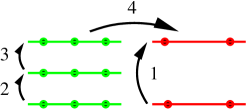
Since a finer grid spacing also requires smaller time steps for hyperbolic problems, the finer grids perform multiple time steps for each coarse grid time step, leading to a recursive time evolution pattern that is typical for Berger-Oliger AMR. If a simulation uses 11 levels, then the resolutions (both in space and time) of the the coarsest and finest levels differ by a factor of . This non-uniform time stepping leads to a certain complexity that is also handled by the Carpet driver; for example, applying boundary conditions to a fine level requires interpolation in space and time from a coarser level. Outputting the solution at a time in between coarse grid time steps also requires interpolation. These parallel interpolation operations are implemented efficiently in Carpet and are applied automatically as specified in the execution schedule, i.e. without requiring function calls in user code. Figure 1 describes some details of the Berger-Oliger time stepping algorithm; more details are described in [108].

Carpet is the main driver used today for Cactus-based astrophysical simulations. Carpet offers hybrid MPI/OpenMP parallelization and is used in production on up to several thousand cores [112, 113].
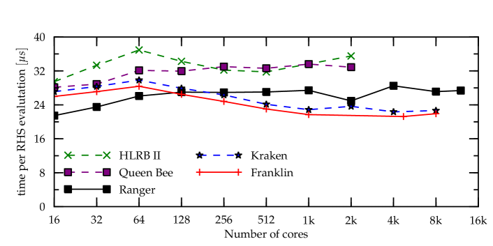
Figure 2 shows a weak scaling test of Carpet, where McLachlan (see section 5.3 below) solves the Einstein equations on a grid structure with nine levels of mesh refinement. This demonstrates excellent scalability up to more than ten thousand cores. In production simulations, smaller and more complex grid structures, serial tasks related to online data analysis and other necessary tasks reduce scalability by up to a factor of ten.
We estimate that in 2010, about 7,000 core years of computing time (45 million core hours) will have been used via Carpet by more than a dozen research groups world-wide. To date, more than 90 peer-reviewed publications and more than 15 student theses have been based on Carpet [110].
4.3 Simulation Factory
Today’s supercomputers differ significantly in their hardware configuration, available software, directory structure, queuing system, queuing policy, and many other user-visible properties. In addition, the system architectures and user interfaces offered by supercomputers are very different from those offered by laptops or workstations. This makes performing large, three-dimensional time-dependent simulations a complex, time-consuming and difficult task. However, most of these differences are only superficial, and the basic capabilities of supercomputers are very similar; most of the complexity of managing simulations lies in menial tasks that require no physical or numerical insight.
The Simulation Factory [114, 115] offers a set of abstractions for the tasks necessary to set up and successfully complete numerical simulations based on the Cactus framework. These abstractions hide tedious low-level management operations, capture “best practices” of experienced users, and create a log trail ensuring repeatable and well-documented scientific results. Using these abstractions, most operations are simplified and many types of potentially disastrous user errors are avoided, allowing different supercomputers to be used in a uniform manner.
Using the Simulation Factory, we offer a tutorial for the Einstein Toolkit [101] that teaches new users how to download, configure, build, and run full simulations of the coupled Einstein/relativistic hydrodynamics equations on a supercomputer with a few simple commands. Users need no prior knowledge about either the details of the architecture of a supercomputer nor its particular software configuration. The same exact set of SimFactory commands can be used on all other supported supercomputers to run the same simulation there.
The Simulation Factory supports and simplifies three kinds of operations:
- 1. Remote Access.
-
The actual access commands and authentication methods differ between systems, as do the user names that a person has on different systems. Some systems are not directly accessible, and one must log in to a particular “trampoline” server first. The Simulation Factory hides this complexity.
- 2. Configuring and Building.
-
Building Cactus requires certain software on the system, such as compilers, libraries, and build tools. Many systems offer different versions of these, which may be installed in non-default locations. Finding a working combination that results in efficient code is extremely tedious and requires low-level system experience. The Simulation Factory provides a machine database that enables users to store and exchange this information. In many cases, this allows people to begin to use a new machine in a very short time with just a few, simple commands.
- 3. Submitting and Managing Simulations.
-
Many simulations run for days or weeks, requiring frequent checkpointing and job re-submission because of short queue run-time limits. Simple user errors in these menial tasks can potentially destroy weeks of information. The Simulation Factory offers safe commands that encapsulate best practices that prevent many common errors and leave a log trail.
The above features make running simulations on supercomputers much safer and simpler.
4.4 Kranc
Kranc[116, 117, 118] is a Mathematica application which converts a high-level continuum description of a PDE into a highly optimized module for Cactus, suitable for running on anything from a laptop to the world’s largest HPC systems. Many codes contain a large amount of complexity, including expanded tensorial expressions, numerical methods, and the large amount of “glue” code needed for interfacing a modern HPC application with the underlying framework. Kranc absorbs this complexity, allowing the scientist to concentrate on writing only the Kranc script which describes the continuum equations.
This approach brings with it many advantages. With these complicated elements factored out, a scientist can write many different Kranc codes, all taking advantage of the features of Kranc and avoiding unnecessary or trivial but painstaking duplication. The codes might be variations on a theme, perhaps versions which use different sets of variables or formulations of the equations, or they could represent completely different physical systems. The use of a symbolic algebra package, Mathematica, enables high-level optimizations which are not performed by the compiler to be implemented in Kranc.
Any enhancements to Kranc can be automatically applied to all codes which are generated using Kranc. Existing codes have easily benefited from the following features added to Kranc after the codes themselves were written: (i) OpenMP parallelization support, necessary for efficient use of modern multi-core processors; (ii) support for multipatch domains with the Llama [119] code; (iii) automatic generation of vectorized code, where the equations are evaluated simultaneously by the processor for two grid points at the same time; and (iv) common sub-expression elimination, and various other optimization strategies.
Within the Einstein Toolkit, the Einstein evolution thorn McLachlan, as well as the wave extraction thorn WeylScal4, are both generated using Kranc, and hence support all the above features.
5 Components
The Einstein Toolkit uses the modular Cactus framework as its underlying infrastructure. A simulation within Cactus could just use one module, but in practice simulations are often composed from hundreds of components. Some of these modules provide common definitions and conventions (see section 5.1). Others provide initial data (see section 5.2), which may be evolved using the different evolution methods for vacuum and matter configurations described in sections 5.3 and 5.4, respectively. The thermodynamic properties of fluids are encoded in equations of state (see section 5.5). Finally, additional quantities which are not directly evolved are often interesting for a detailed analysis of the simulation’s results. Modules providing commonly used analysis methods are described in section 5.6.
5.1 Base Modules
Modular designs have proven to be essential for distributed development of complex software systems and require the use of well-defined interfaces. Low-level interoperability within the Einstein Toolkit is provided by the Cactus infrastructure. One example of this is the usage of one module from within another, e.g., by calling a function within another thorn independent of programming language used for both the calling and called function. Solutions for technical challenges like this can be and are provided by the underlying framework, in this case Cactus.
However, certain other standards are very hard or impossible to enforce on a technical level. Examples for these include the exact definitions of physical variables, their units, and, on a more technical level, the variable names used for the physical quantities. Even distinct simulation codes typically use very similar scheduling schemes, so conventions describing the behavior of the scheduler can help coordinate the order in which functions in different modules are called.
The Einstein Toolkit provides modules whose sole purpose is to declare commonly used variables and define their meaning and units. These conditions are not strictly enforced, but instead documented for the convenience of the user community. Three of these base modules, ADMBase, HydroBase, and TmunuBase, are described in more detail below.
In the following, we assume that the reader is familiar with the basics of numerical relativity and GR hydrodynamics, including the underlying differential geometry and tensor analysis. Detailed introductions to numerical relativity have recently been given by Alcubierre [120], Baumgarte & Shapiro [121], and Centrella et al. [122]. GR hydrodynamics has been reviewed by Font [40]. We set throughout this paper, and where appropriate.
5.1.1 ADMBase
The Einstein Toolkit provides code to evolve the Einstein equations
| (1) |
where is the Einstein tensor, describing the curvature of 4-dimensional spacetime, and is the stress-energy tensor. Relativistic spacetime evolution methods used within the Cactus framework employ different formalisms to accomplish this goal, but essentially all are based on the ADM construction [123], which makes it the natural choice of a common foundation for exchange data between modules using different formalisms. In the approach, 4-dimensional spacetime is foliated into sequences of spacelike 3-dimensional hypersurfaces (slices) connected by timelike normal vectors. The split introduces 4 gauge degrees of freedom: the lapse function that describes the advance of proper time with respect to coordinate time for a normal observer222A normal observer follows a worldline tangent to the unit normal on the 3-hypersurface. and the shift vector that describes how spatial coordinates change from one slice to the next.
According to the ADM formulation, the spacetime metric is assumed to take the form
| (2) |
where , and are the spacetime 4-metric, lapse function, shift vector, and spatial 3-metric, respectively, and we follow the standard relativistic convention where Latin letters are used to index 3-dimensional spatial quantities and Greek letters to index 4-dimensional spacetime quantities, with the index running from 0 to 3. The remaining dynamical component of the spacetime is contained in the definition of the extrinsic curvature , which is defined in terms of the time derivative of the metric after incorporating a Lie derivative with respect to the shift vector:
| (3) |
The three-metric, extrinsic curvature, lapse function, and shift vector are all declared as variables in the ADMBase module, the latter two together with their first time derivatives. The variables provided by ADMBase are:
-
•
The 3-metric tensor, : gxx, gxy, gxz,gyy, gyz, gzz
-
•
The extrinsic curvature tensor, : kxx, kxy, kxz, kyy, kyz, kzz
-
•
The lapse function, : alp
-
•
The shift vector : betax, betay, betaz
This base module also defines common parameters to manage interaction between different modules. Examples are the type of requested initial data or the used evolution method.
The type of initial data chosen for a simulation is specified by the parameters initial_data (3-metric and extrinsic curvature), initial_lapse, initial_shift. The time derivatives of the gauge variables (the lapse and shift) are set by the parameters initial_dtlapse and initial_dtshift, respectively. By default, ADMBase initializes the 3-metric and extrinsic curvature to Minkowski (i.e., , the Kronecker delta, and ), the shift to zero, and the lapse to unity. Initial data thorns override these defaults by extending the parameters.
Analogous to specifying initial data, evolution methods are chosen by the parameters evolution_method (3-metric and extrinsic curvature), lapse_evolution_method, shift_evolution_method, dtlapse_evolution_method and dtshift_evolution_method. ADMBase does not evolve the 3-metric or extrinsic curvature, and holds the lapse and shift static. Evolution thorns extend the ranges of these parameters and contain the evolution code.
The variables defined in ADMBase typically are not used for the actual evolution of the curvature. Instead, it is expected that every evolution module converts its internal representation to the form defined in ADMBase after each evolution step. This procedure enables modules which perform analysis on the spacetime variables to use the ADMBase variables without direct dependency on any of the existing curvature evolution methods.
5.1.2 HydroBase
Similar to ADMBase, the module HydroBase defines a common basis for interactions between modules of a given evolution problem, in this case relativistic hydrodynamics. HydroBase extends the Einstein Toolkit to include an interface within which magnetohydrodynamics may work. HydroBase’s main function is to store variables which are common to most if not all hydrodynamics codes solving the Euler equations, the so-called primitive variables. These are also the variables which are needed to couple to a spacetime solver, and often by analysis thorns as well. As with ADMBase, the usage of a common set of variables by different hydrodynamics codes creates the possibility of sharing parts of the code, e.g., initial data solvers or analysis routines. HydroBase also defines commonly needed parameters and schedule groups for the main functions of a hydrodynamics code.
HydroBase uses a set of conventions known as the Valencia formulation [124, 125, 126]. In particular, HydroBase defines the primitive variables (see [40] for details):
-
•
rho: rest mass density -
•
press: pressure -
•
eps: internal energy density -
•
vel[3]: contravariant fluid three velocity defined as(4) in terms of the four-velocity , lapse, and shift vector .
-
•
Y_e: electron fraction -
•
temperature: temperature -
•
entropy: specific entropy per particle -
•
Bvec[3]: contravariant magnetic field vector defined as(5) in terms of the dual to the Faraday tensor and the unit normal of the foliation of spacetime .
HydroBase also sets up scheduling blocks that organize the main functions which modules of a hydrodynamics code may need. All of those scheduling blocks are optional, but when used they simplify existing codes and make them more interoperable. HydroBase itself does not schedule routines inside most of the groups that it provides. Currently the scheduling blocks are:
-
•
Initializing the primitive variables
-
•
Converting primitive variables to conservative variables
-
•
Calculating the right hand side (RHS) in the method of lines (MoL)
-
•
Setting and updating an excision mask
-
•
Applying boundary conditions
Through these, the initiation of the primitive variables, methods to recover the conservative variables, and basic atmosphere handling can be implemented in different thorns while allowing a central access point for analysis thorns.
5.1.3 TmunuBase
In the Einstein Toolkit, we typically choose the stress energy tensor to be that of an ideal relativistic fluid,
| (6) |
where , , and are defined above, and is the relativistic specific enthalpy.
The thorn TmunuBase provides grid functions for the stress-energy tensor as well as schedule groups to manage when is calculated. In a simulation, many different thorns may contribute to the stress-energy tensor and this thorn allows them to do so without explicit interdependence. The resulting stress-energy tensor can then be used by the spacetime evolution thorn (again without explicit dependence on any matter thorns). When thorn MoL is used for time evolution this provides a high-order spacetime-matter coupling.
The grid functions provided by TmunuBase are:
-
•
The time component : eTtt
-
•
The mixed components : eTtx, eTty, eTtz
-
•
The spatial components : eTxx, eTxy, eTxz, eTyy, eTyz, eTzz
In addition, the grid scalar stress_energy_state has the value 1 if storage is provided for the stress-energy tensor and 0 if not.
Thorn ADMCoupling provides a similar (but older) interface between space-time and matter thorns. However, since it is based on an include file mechanism it is more complicated to use. We recommend all new matter thorns to use TmunuBase instead.
5.2 Initial Data
The Einstein Toolkit contains many modules used to generate initial data for GR simulations, including both vacuum and hydrodynamic configurations. These include modules used primarily for testing of various components, as well as physically motivated configurations that describe, for example, single or binary BHs and/or NSs. Many of the modules are self-contained, consisting of either all the code to generate exact initial solutions or the numerical tools required to construct solutions known semi-analytically. Others, though, require the installation of numerical software packages that are included in the toolkit as external libraries. One example is the TwoPunctures module [127] — commonly used in numerical relativity to generate BH-BH binary initial data — which makes use of the GNU Scientific Library [GSL; [128, 129]]. Several modules have also been implemented to read in data files generated by the Lorene code [130, 131].
Initial data setup is in most cases clearly separated from the evolution that follows. Typically, initial data routines provide the data in terms of the quantities defined in the Base modules (see section 5.1), and the evolution modules will later convert these quantities to forms used for the evolution. For example, an initial data module must supply , the spatial 3-metric, and , the extrinsic curvature. The conversion between the physical metric and extrinsic curvature and conformal versions of these is handled solely within evolution modules, which are responsible for calculating the conformally related three metric , the conformal factor , the conformal traceless extrinsic curvature and the trace of the extrinsic curvature , as well as initializing the BSSN variable should that be the evolution formalism chosen (see section 5.3 for definitions of these). Optionally, many initial data modules also supply values for the lapse and shift vector and in some cases their time derivatives. It is important to note, though, that many dynamical calculations run better from initial gauge choices set by ansatz rather than those derived from stationary approximations that are incompatible with the gauge evolution equations. In particular, conformal thin-sandwich initial data for binaries include solutions for the lapse and shift that are frequently replaced by simpler analytical values that lead to more circular orbits under standard “moving puncture” gauge conditions (see, e.g., [132, 72] and other works).
We turn our attention next to a brief discussion of the capabilities of the aforementioned modules as well as their implementation.
5.2.1 Simple Vacuum initial data
Vacuum spacetime tests in which the constraint equations are explicitly violated are provided by IDConstraintViolate and Exact, a set of exact spacetimes in various coordinates including Lorentz-boosted versions of traditional solutions. Vacuum gravitational wave configurations can be obtained by using either IDBrillData, providing a Brill wave spacetime [133]; or IDLinearWaves, for a spacetime containing a linear gravitational wave. Single BH configurations include IDAnalyticBH which generates various analytically known BH configurations; as well as IDAxibrillBH, IDAxiOddBrillBH, DistortedBHIVP and RotatingDBHIVP, which introduce perturbations to isolated BHs.
5.2.2 Hydrodynamics Tests
Initial data to test different parts of hydrodynamics evolution systems are provided by GRHydro_InitData. This module includes several shock tube problems that may be evolved in any of the Cartesian directions or diagonally. All of these have been widely used throughout the field to evaluate a diverse set of solvers [134]. Conservative to primitive variable conversion and vice versa are also supported, as are tests to check on the reconstruction of hydrodynamical variables at cell faces (see Sec. 5.4 for more on this). Along similar lines, the Hydro_InitExcision module sets up masks for different kinds of excised regions, which is convenient for hydrodynamics tests.
5.2.3 TwoPunctures: Binary Black Holes and extensions
A substantial fraction of the published work on the components of the Einstein toolkit involves the evolution of BH-BH binary systems. The most widely used routine to generate initial data for these is the TwoPunctures code (described originally in [127]) which solves the binary puncture equations for a pair of BHs [135]. To do so, one assumes the extrinsic curvature for each BH corresponds to the Bowen-York form [136]:
| (7) | |||||
where the sub/superscript refers to the contribution from BH ; the 3-momentum is ; the BH spin angular momentum is ; the conformal 3-metric is assumed to be flat, i.e. , and is the Cartesian normal vector relative to the position of each BH in turn. This solution automatically satisfies the momentum constraint, and the Hamiltonian constraint may be written as an elliptic equation for the conformal factor, defined by the condition or equivalently :
| (8) |
Decomposing the conformal factor into a singular analytical term and a regular term , such that
| (9) |
where and are the mass of and distance to each BH, respectively, and is defined by the equation itself, the Hamiltonian constraint may be written as
| (10) |
subject to the boundary condition as . In Cartesian coordinates, the function is infinitely differentiable everywhere except the two puncture locations. TwoPunctures resolves this problem by performing a coordinate transformation modeled on confocal elliptical/hyperbolic coordinates. This transforms the spatial domain into a finite cube with the puncture locations mapped to two parallel edges, as can be seen in figure 3. The coordinate transformation is:
| (11) |
which maps onto (the elliptical quasi-radial coordinate), (the hyperbolic quasi-latitudinal coordinate), and (the longitudinal angle). Since is smooth everywhere in the interior of the remapped domain, expansions into modes in these coordinates are spectrally convergent and thus capable of extremely high accuracy. In practice, the field is expanded into Chebyshev modes in the quasi-radial and quasi-latitudinal coordinates, and into Fourier modes around the axis connecting the two BHs. The elliptic solver uses a stabilized biconjugate gradient method to achieve rapid solutions and to avoid ill-conditioning of the spectral matrix.

5.2.4 Lorene-based binary data
The ET contains three routines that can read in publicly available data generated by the Lorene code [130, 131], though it does not currently include the capability of generating such data from scratch. For a number of reasons, such functionality is not truly required; in particular, Lorene is a serial code and to call it as an ET initial data generator saves no time. Also, it is not guaranteed to be convergent for an arbitrary set of parameters; thus the initial data routine itself may never finish its iterative steps. Instead, recommended practice is to let Lorene output data into files, and then read those into ET at the beginning of a run.
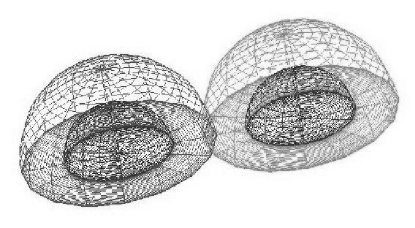
Lorene uses a multigrid spectral approach to solve the conformal thin-sandwich equations for binary initial configurations [132] and a single-grid spectral method for rotating stars. For binaries, five elliptic equations for the shift, lapse, and conformal factor are written down and the source terms are divided into pieces that are attributed to each of the two objects. Matter source terms are ideal for this split, since they are compactly supported, while extrinsic curvature source terms are spatially extended but with sufficiently rapid falloff at large radii to yield convergent solutions. Around each object, a set of nested spheroidal sub-domains (see figure 4) is constructed to extending through all of space, with the outermost domain incorporating a compactification to allow it to extend to spatial infinity. Within each of the nested sub-domains, fields are decomposed into Chebyshev modes radially and into spherical harmonics in the angular directions, with elliptic equation solving reduced to a matrix problem. The nested sub-domains need not be perfectly spherical, and indeed one may modify the outer boundaries of each to cover any convex shape. For NSs, this allows one to map the surface of a particular sub-domain to the NS surface, minimizing Gibbs error there. For BHs, excision boundary conditions are imposed at the horizon. To read a field solution describing a given quantity onto a Cactus-based grid, one must incorporate the data from each star’s domains at that point.
5.2.5 TOVSolver
The TOVSolver routine in the ET solves the standard TOV equations [138, 139] expressed using the Schwarzschild (areal) radius in the interior of a spherically symmetric star in hydrostatic equilibrium:
| (12) |
where is the energy density of the fluid, including the internal energy contribution111We note that since different application thorns may define their own local variables, the energy density is referred to as rho within TOVSolver, as the projected energy density , defined in Sec. 5.3, is within McLachlan and a few other thorns. Similar ambiguities exist for other commonly used variable names, particularly and ., is the gravitational mass inside a sphere of radius , and the logarithm of the lapse. The routine also supplies the analytically known solution in the exterior,
| (13) |
where TOV_atmosphere is a parameter used to define the density of the ambient atmosphere. Since the isotropic radius is the more commonly preferred choice to initiate dynamical calculations, the code then transforms all variables into isotropic coordinates, integrating the radius conversion formula
| (14) |
subject to the boundary condition that in the exterior,
| (15) |
handling with some care the potentially singular terms that appear at the origin.
To facilitate the construction of stars in more complicated dynamical configurations, one may also apply a uniform velocity to the NS, though this does not affect the ODE solution nor the resulting density profile.
5.3 Spacetime Curvature Evolution
The Einstein Toolkit curvature evolution code McLachlan [140, 112] is auto-generated from tensor equations via Kranc (Sec. 4.4). It implements the Einstein equations in a split as a Cauchy initial boundary value problem [141]. For this, the Baumgarte-Shapiro-Shibata-Nakamura (BSSN) conformal-tracefree reformulation [9, 10, 142] of the original Arnowitt-Deser-Misner (ADM) formalism [123] is employed. McLachlan uses fourth-order accurate finite differencing for the spacetime variables and adds a fifth-order Kreiss-Oliger dissipation term to remove high frequency noise. The evolved variables are the conformal factor , the conformal 3-metric , the trace of the extrinsic curvature, the trace free extrinsic curvature and the conformal connection functions . These are defined in terms of the standard ADM 4-metric , 3-metric , and extrinsic curvature by:
| (16) | |||||
| (17) | |||||
| (18) | |||||
| (19) | |||||
| (20) |
The evolution equations are then:
| (21) | |||||
| (22) | |||||
| (23) | |||||
| (24) | |||||
| (25) | |||||
| (26) | |||||
| (27) | |||||
| (28) | |||||
with the momentum constraint damping constant set to . The stress energy tensor is incorporated via the projections
| (29) | |||||
| (30) | |||||
| (31) |
We have introduced the notation . All quantities with a tilde involve the conformal 3-metric , which is used to raise and lower indices. In particular, and refer to the covariant derivative and the Christoffel symbols with respect to . The expression denotes the trace-free part of the expression inside the parentheses, and we define the Ricci tensor contributions as:
| (32) | |||||
| (33) |
This is a so-called -variant of BSSN. The evolved gauge variables are lapse , shift , and a quantity related to the time derivative of the shift. The gauge parameters , , , and are determined by our choice of a [143] slicing:
| (34) | |||||
| (35) |
and -driver shift condition [143]:
| (36) | |||||
| (37) | |||||
| (38) |
The expression attenuates the -driver depending on the radius as described below.
The -driver shift condition is symmetry-seeking, driving the shift to a state that renders the conformal connection functions stationary. Of course, such a stationary state cannot be achieved while the metric is evolving, but in a stationary spacetime the time evolution of the shift and thus that of the spatial coordinates will be exponentially damped. This damping time scale is set by the gauge parameter (see (38)) which has dimension (inverse time). As described in [144, 145], this time scale may need to be adapted in different regions of the domain to avoid spurious high-frequency behavior in regions that otherwise evolve only very slowly, e.g., far away from the source.
Here we use the simple damping mechanism described in (12) of [145], which is defined as:
| (41) |
with a constant defining the transition radius between the interior, where , and the exterior, where falls off as . A description of how appears in the gauge parameters may be found in (38).
5.3.1 Initial Conditions
Initial conditions for the ADM variables , , lapse , and shift are provided by the initial data routines discussed in Sec. 5.2. From these the BSSN quantities are calculated via their definitions, setting , and using cubic extrapolation for at the outer boundary. This extrapolation is necessary since the are calculated from derivatives of the metric, and one cannot use centered finite differencing stencils near the outer boundary.
The extrapolation stencils distinguish between points on the faces, edges, and corners of the grid. Points on the faces are extrapolated via stencils perpendicular to that face, while points on the edges and corners are extrapolated with stencils aligned with the average of the normals of the adjoining faces. For example, points on the edge are extrapolated in the direction, while points in the corner are extrapolated in the direction. Since several layers of boundary points have to be filled for higher order schemes (e.g., three layers for a fourth order scheme), one proceeds outwards starting from the innermost layer. Each subsequent layer is then defined via the points in the interior and the previously calculated layers.
5.3.2 Boundary Conditions
During time evolution, a Sommerfeld-type radiative boundary condition is applied to all components of the evolved BSSN variables as described in [142]. The main feature of this boundary condition is that it assumes approximate spherical symmetry of the solution, while applying the actual boundary condition on the boundary of a cubic grid where the face normals are not aligned with the radial direction. This boundary condition defines the right hand side of the BSSN state vector on the outer boundary, which is then integrated in time as well so that the boundary and interior are calculated with the same order of accuracy.
The main part of the boundary condition assumes that one has an outgoing radial wave with some speed :
| (42) |
where is any of the tensor components of evolved variables, the value at infinity, and a spherically symmetric perturbation. Both and depend on the particular variable and have to be specified. This implies the following differential equation:
| (43) |
where . The spatial derivatives are evaluated using centered finite differencing where possible, and one-sided finite differencing elsewhere. Second order stencils are used in the current implementation.
In addition to this main part, it is also necessary to account for those parts of the solution that do not behave as a pure wave, e.g., Coulomb type terms caused by infall of the coordinate lines. It is assumed that these parts decay with a certain power of the radius. This is implemented by considering the radial derivative of the source term above, and extrapolating according to this power-law decay.
Given a source term , one defines the corrected source term via
| (44) |
where is the normal vector of the corresponding boundary face. The spatial derivatives are evaluated by comparing neighboring grid points, corresponding to a second-order stencil evaluated in the middle between the two neighboring grid points. Second-order decay is assumed, hence .
As with the initial conditions above, this boundary condition is evaluated on several layers of grid points, starting from the innermost layer. Both the extrapolation and radiative boundary condition algorithms are implemented in the publicly available NewRad component of the Einstein Toolkit.
This boundary condition is only a coarse approximation of the actual decay behavior of the BSSN state vector, and it does not capture the correct behavior of the evolved variables. However, one finds that this boundary condition leads to stable evolutions if applied sufficiently far from the source. Errors introduced at the boundary (both errors in the geometry and constraint violations) propagate inwards with the speed of light [140]. Gauge changes introduced by the boundary condition, which are physically not observable, propagate faster, with a speed up to for the gauge conditions used in McLachlan.
5.4 Hydrodynamics Evolution
Hydrodynamic evolution in the Einstein Toolkit is designed so that it interacts with the metric curvature evolution through a small set of variables, allowing for maximum modularity in implementing, editing, or replacing either evolution scheme.
The primary hydrodynamics evolution routine in the Einstein Toolkit is GRHydro, a code derived from the public Whisky code [94, 146, 147, 148] designed primarily by researchers at AEI and their collaborators. It includes a high resolution shock capturing (HRSC) scheme to evolve hydrodynamic quantities, with several different reconstruction methods and Riemann solvers, as we discuss below. In such a scheme, we define a set of “conserved” hydrodynamic variables, defined in terms of the “primitive” physical variables such as mass and internal energy density, pressure, and velocity. Wherever derivatives of hydrodynamic terms appear in the evolution equations for the conserved variables, they are restricted to appear only inside divergence terms (referred to as fluxes) and never in the source terms. By calculating fluxes at cell faces, we may obtain a consistent description of the inter-cell values using reconstruction techniques that account for the fact that hydrodynamic variables are not smooth and may not be finite differenced accurately. All other source terms in the evolution equations may contain only the hydrodynamic variables themselves and the metric variables and derivatives of the latter, since the metric must formally be smooth and thus differentiable using finite differencing techniques. Summarizing these methods briefly, the following stages occur every timestep:
-
•
The primitive variables are “reconstructed” at cell faces using shock-capturing techniques, with total variation diminishing (TVD), piecewise parabolic (PPM), and essentially non-oscillatory (ENO) methods currently implemented.
-
•
A Riemann problem is solved at each cell face using an approximate solver. Currently implemented versions include HLLE (Harten-Lax-van Leer-Einfeldt), Roe, and Marquina solvers.
-
•
The conserved variables are advanced one timestep, and used to recalculate the new values of the primitive variables.
We discuss the GRHD formalism, the stages within a timestep, and the other aspects of the code below, noting that the documentation included in the released version is quite extensive and covers many of these topics in substantially more detail.
5.4.1 Ideal general relativistic hydrodynamics (GRHD)
The equations of ideal GR hydrodynamics evolved by GRHydro are derived from the local GR conservation laws of mass and energy-momentum:
| (45) |
where denotes the covariant derivative with respect to the 4-metric, and is the mass current.
The 3-velocity may be calculated in the form
| (46) |
where is the Lorentz factor. The contravariant 4-velocity is then given by:
| (47) |
and the covariant 4-velocity is:
| (48) |
The GRHydro evolution scheme is a first-order hyperbolic flux-conservative system for the conserved variables , , and , which may be defined in terms of the primitive variables , such that:
| (49) | |||||
| (50) | |||||
| (51) |
where is the determinant of . The evolution system then becomes
| (52) |
with
| (53) | |||||
Here, and are the 4-Christoffel symbols. The time integration and coupling with curvature are carried out with the Method of Lines [149]. The expressions for are calculated in GRHydro by using the definition of the extrinsic curvature to avoid any time derivatives whatsoever, as discussed in detail in the code’s documentation, following a suggestion by Mark Miller based on experience with the GR3D code.
5.4.2 Reconstruction techniques
In order to calculate fluxes at cell faces, we first must calculate function values on either side of the face. In practice, reconstructing the primitive variables yields more stable and accurate evolutions than reconstructing the conservatives. In what follows, we assume a Cartesian grid and loop over faces along each direction in turn. We define to be the value of a quantity on the left side of the face between and , where is the th point in the -direction, and the right side of the same face.
For total variation diminishing (TVD) methods, we let:
| (54) |
where is a slope-limited gradient function, typically determined by the values of and , with a variety of different forms of the slope limiter available. In practice, all try to accomplish the same task of preserving monotonicity and removing the possibility of spuriously creating local extrema. Implemented methods include minmod, superbee [150], and monotonized central [151].
The piecewise parabolic method (PPM) is a multi-step method based around a quadratic fit to nearby points interpolated to cell faces [152], for which and are generally equivalent except near shocks and local extrema. The version implemented in GRHydro includes the steepening and flattening routines described in the original PPM papers, with a simplified dissipation procedure. Essentially non-oscillatory (ENO) methods use a divided differences approach to achieve third-order accuracy via polynomial interpolation [153, 154].
Both ENO and PPM yield third-order accuracy for smooth monotonic functions, whereas TVD methods typically yield second-order accurate values. Regardless of the reconstruction scheme chosen, all of these methods reduce to first order near local extrema and shocks.
5.4.3 Riemann solvers
The Riemann problem involves the solution of the equation
| (55) |
at some point representing a discontinuity between constant states. The exact solution can be quite complicated, involving five different waves with different characteristic speeds for a hydrodynamic problem (8 for GRMHD), so GRHydro implements three different approximate solvers to promote computational efficiency. In each case, the solution takes a self-similar form , where represents the characteristic speed from the original shock location to the point in question in space and time.
The simplest method implemented is the Harten-Lax-van Leer-Einfeldt solver [155, 156] (HLL or HLLE, depending on the reference), which uses a two wave approximation to calculate the evolution along the shock front. With and the most negative and most positive wave speeds present on either side of the interface, the solution is assumed to take the form
| (56) |
with the intermediate state given by
| (57) |
The numerical flux along the interface takes the form
| (58) |
where
| (59) |
It is these flux terms that are then used to evolve the hydrodynamic quantities.
The Roe solver [157] involves linearizing the evolution system for the hydrodynamic evolution, defining the Jacobian matrix (see (55)), and working out the eigenvalues and left and right eigenvectors, and , assumed to be orthonormalized so that . Defining the characteristic variables , the characteristic equation becomes
| (60) |
with the diagonal matrix of eigenvalues. Letting represent the differences in the characteristic variables across the interface, the Roe flux is calculated as
| (61) |
where the eigenvector appearing in the summed term are evaluated for the approximate Roe average flux . The Marquina flux routines use a similar approach to the Roe method, but provide a more accurate treatment for supersonic flows (i.e., those for which the characteristic wave with is within a rarefaction zone) [158, 159].
5.4.4 Conservative to primitive conversion
In order to invert eqs. (49) – (51), solving for the primitive variables based on the values of the conservative ones, GRHydro uses a 1-dimensional Newton-Raphson approach that solves for a consistent value of the pressure. Defining the (known) undensitized conservative variables , and , as well as the auxiliary quantities and , the former of which depends on and the latter of which is known, we find that and thus
| (62) | |||||
| (63) | |||||
| (64) |
Given the new values of and , one may then find the residual between the pressure and and perform the Newton-Raphson step, so long as the values of and are known.
5.4.5 Atmospheres, boundaries, and other code details
GRHydro uses an atmosphere, or extremely-low density floor, to avoid problems involving sound speeds and conservative-to-primitive variable conversion near the edges of matter distributions. The floor density value may be chosen in either absolute (rho_abs_min) or relative (rho_rel_min) terms. The atmosphere is generally assumed to have a specified polytropic EOS, regardless of the EOS describing the rest of the matter within the simulation. Whenever the numerical evolution results in a grid cell where conservative to primitive variable conversion yields negative values of either or , the cell is reassigned to the atmosphere, with zero velocity.
At present, only flat boundary conditions are supported for hydrodynamic variables, since it is generally recommended that the outer boundaries of the simulation be placed far enough away so that all cells near the edge of the computational domain represent the atmosphere.
GRHydro has the ability to advect a set of passive scalars, referred to as “tracers”, as well as the electron fraction of a fluid, under the assumption that each tracer follows the conservation law
| (65) |
5.5 Equations of State
An equation of state connecting the primitive state variables is needed to close the system of GR hydrodynamics equations. The module EOS_Omni provides a unified general equation of state (EOS) interface and back-end for simple analytic and complex microphysical EOSs.
The polytropic EOS
| (66) |
where is the polytropic constant and is the adiabatic index, is appropriate for adiabatic (= isentropic) evolution without shocks. When using the polytropic EOS, one does not need to evolve the total fluid energy equation, since the specific internal energy is fixed to
| (67) |
Note that the adiabatic index is related to the frequently used polytropic index via .
The gamma-law EOS333For historic reasons, this EOS is referred to as the “ideal fluid” EOS in GRHydro.,
| (68) |
allows for non-adiabatic flow but still assumes fixed microphysics, which is encapsulated in the constant adiabatic index . This EOS has been used extensively in simulations of NS-NS and BH-NS mergers.
The hybrid EOS, first introduced by [160], is a 2-piecewise polytropic with a thermal component designed for the application in simple models of stellar collapse. At densities below nuclear density, a polytropic EOS with is used. To mimic the stiffening of the nuclear EOS at nuclear density, the low-density polytrope is fitted to a second polytrope with . To allow for thermal contributions to the pressure due to shock heating, a gamma-law with is used. The full EOS then reads
| (69) | |||||
In this, the total specific internal energy consists of a polytropic and a thermal contribution. In iron core collapse, the pressure below nuclear density is dominated by the pressure of relativistically degenerate electrons. For this, one sets [cgs] in the above. The thermal index is usually set to , corresponding to a mixture of relativistic () and non-relativistic () gas. Provided appropriate choices of EOS parameters (e.g., [161]), the hybrid EOS leads to qualitatively correct collapse and bounce dynamics in stellar collapse.
EOS_Omni also integrates the nuc_eos driver routine, which was first developed for the GR1D code [49] for tabulated microphysical finite-temperature EOS which assume nuclear statistical equilibrium (NSE). nuc_eos handles EOS tables in HDF5 format which contain entries for thermodynamic variables , where is the matter temperature and is the electron fraction. nuc_eos also supports calls for and carries out a Newton iteration to find . For performance reasons, nuc_eos employs simple tri-linear interpolation in thermodynamic quantities and thus requires finely spaced tables to maintain thermodynamic consistency at an acceptable level. EOS tables in the format required by nuc_eos are freely available from http://stellarcollapse.org.
5.6 Analysis
It is often beneficial and sometimes necessary to evaluate analysis quantities during the simulation rather than post-processing variable output. Beyond extracting physics, these quantities are often used as measures of how accurately the simulation is progressing. In the following, we describe the common quantities available through Einstein Toolkit modules, and how different modules approach these quantities with differing assumptions and algorithms. The most common analysis quantities provided fall broadly into several different categories, including horizons, masses and momenta, and gravitational waves. Note that several modules bridge these categories and some fall outside them, including routines to perform constraint monitoring and to compute commonly used derived spacetime quantities. The following discussion is meant as an overview of the most common tools rather than an exhaustive list of the functionality provided by the Einstein Toolkit. In most cases, the analysis modules work on the variables stored in the base modules discussed in Sec. 5.1, ADMBase, TmunuBase, and HydroBase, to be as portable as possible.
5.6.1 Horizons
When spacetimes contain a BH, localizing its horizon is necessary for describing time-dependent quasi-local measures such as its mass and spin. The Einstein Toolkit provides two modules — AHFinder and AHFinderDirect — for locating the apparent horizons (AHs) defined locally on a hypersurface. The module EHFinder is also available to search an evolved spacetime for the globally defined event horizons.
EHFinder [162] evolves a null surface backwards in time given an initial guess (e.g., the last apparent horizon) which will, in the vicinity of an event horizon, converge exponentially to its location. This must be done after a simulation has already evolved the initial data forward in time with enough 3D data written out that the full 4-metric can be recovered at each timestep.
In EHFinder, the null surface is represented by a function which is required to satisfy the null condition . In the standard numerical 3+1 form of the metric, this null condition can be expanded out into an evolution equation for as
| (70) |
where the roots are chosen to describe outgoing null geodesics. The function is chosen such that it is negative within the initial guess of the horizon and positive outside, initially set to a distance measure from the initial surface guess . There is a numerical problem with the steepening of during the evolution, so the function is regularly re-initialized during the evolution to satisfy . This is done by evolving
| (71) |
for some unphysical parameter until a steady state has been reached. As the isosurface converges exponentially to the event horizon, it is useful to evolve two such null surfaces which bracket the approximate position of the anticipated event horizon to further narrow the region containing the event horizon.
However, event horizons can only be found after the full spacetime has been evolved. It is often useful to know the positions and shapes of any BH on a given hypersurface for purposes such as excision, accretion, and local measures of its mass and spin. The Einstein Toolkit provides several algorithms of varying speed and accuracy to find marginally trapped surfaces, of which the outermost are AHs. All finders make use of the fact that null geodesics have vanishing expansion on an AH which, in the usual 3+1 quantities, can be written
| (72) |
where is the unit outgoing normal to the 2-surface.
The module AHFinder provides two algorithms for locating AHs. The minimization algorithm [163] finds the local minimum of corresponding to a surface of constant expansion , with corresponding to the AH. For time-symmetric data, the option exists to find instead the minimum of the surface area, which in this case corresponds to an AH. An alternative algorithm provided by AHFinder, the flow algorithm [164], on which EHFinder is also based. Defining a surface as a level set , and introducing an unphysical timelike parameter to parametrize the flow of towards a solution, (72) can be rewritten
| (73) |
where is a strictly positive weight, is the Laplacian of the 2D metric, and , , and are free parameters. Decomposing onto a basis of spherical harmonics, the coefficients evolve iteratively towards a solution as
| (74) |
The AHFinderDirect module [165] is a faster alternative to AHFinder. Its approach is to view (72) as an elliptic PDE for on using standard finite differencing methods. Rewriting (72) in the form
| (75) |
the expansion is evaluated on a trial surface, then iterated using a Newton-Raphson method to solve , where is the Jacobian matrix. The drawback of this method is that it is not guaranteed to give the outermost marginally trapped surface. In practice however, this limitation can be easily overcome by either a single good initial guess, or multiple less accurate initial guesses.
5.6.2 Masses and Momenta
Two distinct measures of mass and momenta are available in relativistic spacetimes. First, ADM mass and angular momentum evaluated as either surface integrals at infinity or volume integrals over entire hypersurfaces give a measure of the total energy and angular momentum in the spacetime. The module ML_ADMQuantities of the McLachlan code [166] uses the latter method, creating gridfunctions containing the integrand of the volume integrals [167]:
| (76) | |||||
| (77) |
on which the user can use the reduction functions provided by Carpet to perform the volume integral. We note that ML_ADMQuantities inherits directly from the BSSN variables stored in McLachlan rather than strictly from the base modules. As the surface terms required when converting a surface integral to a volume integral are neglected, this procedure assumes that the integrals of and over the boundaries of the computational domain vanish. The ADM mass and angular momentum can also be calculated from the variables stored in the base modules using the Extract module, as surface integrals [136]
| (78) | |||||
| (79) |
on a specified spherical surface, preferably one far from the center of the domain since these quantities are only properly defined when calculated at infinity.
There are also the quasi-local measures of mass and angular momentum, from any AHs found during the spacetime. Both AHFinderDirect and AHFinder output the corresponding mass derived from the area of the horizon .
The module QuasiLocalMeasures implements the calculation of mass and spin multipoles from the isolated and dynamical horizon formalism [168, 169], as well as a number of other proposed formulæ for quasilocal mass, linear momentum and angular momentum that have been advanced over the years [170]. Even though there are only a few rigorous proofs that establish the properties of these latter quantities, they have been demonstrated to be surprisingly helpful in numerical simulations (see, e.g., [171]), and are therefore an indispensable tool in numerical relativity. QuasiLocalMeasures takes as input a horizon surface, or any other surface that the user specifies (like a large coordinate sphere) and can calculate useful quantities such as the Weyl or Ricci scalars or the three-volume element of the horizon world tube in addition to physical observables such as mass and momenta.
Finally, the module HydroAnalysis additionally locates the (coordinate) center of mass as well as the point of maximum rest mass density of a matter field.
5.6.3 Gravitational Waves
One of the main goals of numerical relativity to date is modeling gravitational waveforms that may be used in template generation to help analyze data from the various gravitational wave detectors around the globe. The Einstein Toolkit includes modules for extracting gravitational waves via either the Moncrief formalism of a perturbation on a Schwarzschild background or the calculation of the Weyl scalar .
The module Extract uses the Moncrief formalism [172] to extract gauge-invariant wave functions and given spherical surfaces of constant coordinate radius. The spatial metric is expressed as a perturbation on Schwarzschild and expanded into a tensor basis of the Regge-Wheeler harmonics [173] described by six standard Regge-Wheeler functions . From these basis functions the gauge-invariant quantities:
| (80) | |||||
| (81) | |||||
are calculated, where and . These functions then satisfy the wave equations:
| (82) | |||||
| (83) | |||||
where . Since these functions describe the 4-metric as a perturbation on Schwarzschild, the spacetime must be approximately spherically symmetric for the output to be interpreted as first-order gauge-invariant waveforms.
For more general spacetimes, the module WeylScal4 calculates the complex Weyl scalar , which is a projection of the Weyl tensor onto components of a null tetrad. WeylScal4 uses the fiducial tetrad [174], written in 3+1 decomposed form as:
| (84) | |||||
| (85) | |||||
| (86) |
where is the unit normal to the hypersurface. The spatial vectors are created by initializing , , and , then orthonormalizing starting with and invoking a Gram-Schmidt procedure at each step to ensure the continued orthonormality of this spatial triad.
The Weyl scalar is calculated explicitly in terms of projections of the 3-Riemann tensor onto a null tetrad, such that
| (87) | |||||
For a suitably chosen tetrad, this scalar in the radiation zone is related to the strain of the gravitational waves since
| (88) |
While the waveforms generated by Extract are already decomposed on a convenient basis to separate modes, the complex quantity is provided by WeylScal4 as a complex grid function. For this quantity, and any other real or complex grid function, the module Multipole interpolates the field onto coordinate spheres of given radii and calculates the coefficients
| (89) |
of a projection onto spin-weighted spherical harmonics .
5.6.4 Object tracking
We provide a module (PunctureTracker) for tracking BH positions evolved with moving puncture techniques. It can be used with (CarpetTracker) to have the mesh refinement regions follow the BHs as they move across the grid. The BH position is stored as the centroid of a spherical surface (even though there is no surface) provided by SphericalSurface.
Since the punctures only move due to the shift advection terms in the BSSN equations, the puncture location is evolved very simply as
| (90) |
where is the puncture location and is the shift. Since the puncture location usually does not coincide with grid points, the shift is interpolated to the location of the puncture. Equation ((90)) is implemented with a simple first-order Euler scheme, accurate enough for controlling the location of the mesh refinement hierarchy.
Another class of objects which often needs to be tracked are neutron stars. Here is it usually sufficient to locate the position of the maximum density and adapt AMR resolution in these regions accordingly, coupled with the condition that this location can only move at a specifiable maximum speed.
5.6.5 Other analysis modules
The remaining analysis capabilities of the Einstein Toolkit span a variety of primarily vacuum-based functions. First, modules are provided to calculate the Hamiltonian and momentum constraints which are used to monitor how well the evolved spacetime satisfies the Einstein field equations. Two modules, ADMConstraints and ML_ADMConstraints provide these quantities. Both calculate these directly from variables stored in the base modules described in Sec. 5.1, explicitly written as:
| (91) | |||||
| (92) |
where . The difference between these modules lies in how they access the stress energy tensor , as the module ADMConstraints uses a deprecated functionality which does not require storage for .
Finally, ADMAnalysis calculates a variety of derived spacetime quantities that are often useful in post-processing such as the determinant of the 3-metric , the trace of the extrinsic curvature , the 3-Ricci tensor in Cartesian coordinates and its trace , as well as the 3-metric and extrinsic curvature converted to spherical coordinates.
5.7 Simulation Domain, Symmetries, Boundaries
5.7.1 Domains and Coordinates.
Cactus distinguishes between the physical domain, which lives in the continuum, and discrete domain, which consists of a discrete set of grid points. The physical domain is defined by its coordinate extent and is independent of the numerical resolution; in particular, the boundary of the physical domain has a width of zero (and is thus a set of measure zero). The discrete domain is defined indirectly via a discretization procedure that specifies the number of boundary points, their location with respect to the physical boundary, and either the grid spacing or the number of grid points spanning the domain. This defines the number and location of the grid points in the discrete domain. The discrete domain may have grid points outside of the physical domain, and may have a non-zero boundary width. This mechanism ensures that changes in the numerical resolution do not affect the extent of the physical domain, i.e., that the discrete domains converge to the physical domain in the limit of infinite resolution. The Einstein Toolkit provides the CoordBase thorn that facilitates the definition of the simulation domain independent of the actual evolution thorn used, allowing it to be specified at run time via parameters in the same way that parameters describing the physical system are specified. CoordBase exposes a public runtime interface that allows other thorns to query the domain description in a uniform way. This is used by Carpet to query CoordBase for the discrete grid when creating the hierarchy of grids, automatically ensuring a consistent grid description between the two thorns. Evolution thorns such as McLachlan use the domain information to decide which points are evolved and therefore require the evaluation of the right-hand-side expression, and which ones are set via boundary or symmetry conditions.
5.7.2 Symmetries and Boundary Conditions.
The Einstein Toolkit includes two thorns, Boundary and SymBase, to provide a generic interface to specify and implement boundary and symmetry conditions. The toolkit includes built-in support for a set of reflecting or rotating symmetry conditions that can be used to reduce the size of the simulation domain. These symmetries include periodicity in any of the coordinate directions (via the Periodic module), reflections across the coordinate planes (via the Reflection module), and rotational symmetries (via the RotatingSymmetry90 and RotatingSymmetry180 modules respectively) about the axis, and a continuous rotational symmetry (via the Cartoon2D thorn) [175]. Cartoon2D allows fully three dimensional codes to be used in axisymmetric problems by evolving a slice in the plane and using the rotational symmetry to populate ghost points off the plane (see Figure 5).

In applying symmetries to populate ghost zones, the transformation properties of tensorial quantities (including tensor densities and non-tensors such as Christoffel symbols) are correctly taken into account, just as they are in the interpolation routines present in Cactus. Thus, symmetries are handled transparently from the point of view of user modules (see Figure 6 for an illustration).
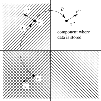
The Boundary thorn serves as a registry for available boundary conditions and provides basic scheduling to enforce all requested boundary conditions at the proper times. It also provides a basic set of boundary conditions to be used by user thorns. The “flat” boundary conditions often used for hydrodynamic variables that approach an atmosphere value fall in this category. More complicated boundary conditions are often implemented as modifications to the evolution equations and are not handled directly by Boundary. Examples are the radiative (Sommerfeld) and extrapolation boundary conditions provided by thorn NewRad.
5.7.3 Adaptive Mesh Refinement
The Einstein toolkit currently supports feature-based mesh refinement, which is based on extracting quantities such as the locations of BHs or NSs and then constructing a mesh hierarchy (stacks of refined regions) based on the locations, sizes, and speeds of these objects. This allows tracking objects as they move through the domain. One can also add or remove stacks if, for instance, the number of objects changes. Full AMR based on a local error estimate is supported by Carpet, but the Einstein Toolkit does not presently provide a suitable regridding thorn to create such a grid. If initial conditions are constructed outside of Carpet (which is often the case), then the initial mesh hierarchy has to be defined manually. In order to facilitate the description of the mesh hierarchy the Einstein toolkit provides two regridding modules in the CarpetRegrid and CarpetRegrid2 thorns. Both thorns primarily support box-in-box type refined meshes, which are well suited to current binary BH simulations in which the high-resolution regions are centered on the individual BHs. Figure 7 shows a typical set of nested boxes during the inspiral phase of a binary BH merger simulation.

CarpetRegrid provides a number of different ways to specify the refined regions, e.g., as a set of boxes centered around the origin or as an explicit list of regions that make up the grid hierarchy. Traditionally, groups using CarpetRegrid have employed auxiliary thorns that are not part of the Einstein Toolkit to create this list of boxes based on information obtained from apparent horizon tracking or other means. CarpetRegrid2 provides a user-friendly interface to define sets of nested boxes that follow BHs or other tracked objects. Object coordinates are updated by CarpetTracker, which provides a simple interface to the object trackers PunctureTracker and NSTracker (see section 5.6.4) in order to have the refined region follow the moving objects. CarpetRegrid2 contains code to handle the -symmetry provided by RotatingSymmetry180, enforcing the symmetry on the resulting grid layout (see Figure 8).
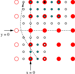
6 Examples
To demonstrate the properties of the code and its capabilities, we have used it to simulate common astrophysical configurations of interest. Given the community-oriented direction of the project, the parameter files required to launch these simulations and a host of others are included and documented in the code releases, along with the data files produced by a representative set of simulation parameters to allow for code validation and confirmation of correct code performance on new platforms and architectures. As part of the internal validation process, nightly builds are checked against a set of benchmarks to ensure that consistent results are generated with the inclusion of all new commits to the code.
The performance of the Toolkit for vacuum configurations is demonstrated through evolutions of single, rotating BHs and the merger of binary black hole configurations (sections 6.1 and 6.2, respectively). Linear oscillations about equilibrium for an isolated NS are discussed in section 6.3, and the collapse of a NS to a BH, including dynamical formation of a horizon, in section 6.4. Finally, to show a less traditional application of the code, we show its ability to perform cosmological simulations by evolving a Kasner spacetime (see section 6.5).
6.1 Spinning BH
As a first example, we perform simulations of a single distorted rotating BH. We use TwoPunctures to set up initial data for a single puncture of mass and dimensionless spin parameter . Evolution of the data is performed by McLachlan, apparent horizon finding by AHFinderDirect and gravitational wave extraction by WeylScal4 and Multipole. Additional analysis of the horizons is done by QuasiLocalMeasures. The runs were performed with fixed mesh refinement provided by Carpet, using 8 levels of refinement on a quadrant grid (symmetries provided by ReflectionSymmetry and RotatingSymmetry180). The outer boundaries were placed at . We performed runs at 3 different resolutions: the low resolution was , medium was and high was , where the numbers refer to the resolution on the finest (coarsest) grid. The runs where performed using the tapering evolution scheme in Carpet to avoid interpolation in time during prolongation. The initial data corresponds to a rotating BH perturbed by a Brill wave and, as such, has a non-zero gravitational wave content. We evolved the BH using 4th-order finite differencing from until it had settled down to a stationary state at .
Figure 9 shows the mode of extracted at , and its numerical convergence.
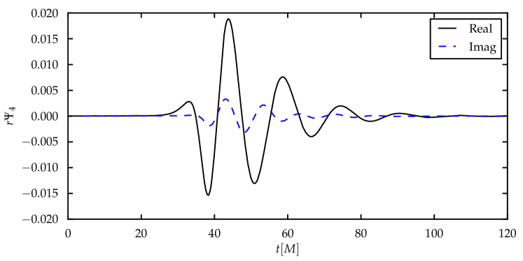
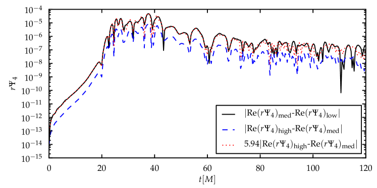
In the top plot the black (solid) curve is the real part and the blue (dashed) curve is the imaginary part of for the high resolution run. Curves from the lower resolution are indistinguishable from the high resolution curve at this scale. In the bottom plot the black (solid) curve shows the absolute value of the difference between the real part of the medium and low resolution waveforms while the blue (dashed) curve shows the absolute value of the difference between the high and medium resolution waveforms in a log-plot. The red (dotted) curve is the same as the blue (dashed) curve, except it is scaled for 4th order convergence. With the resolutions used here this factor is .
Figure 10 shows similar plots for the mode of , again extracted at .
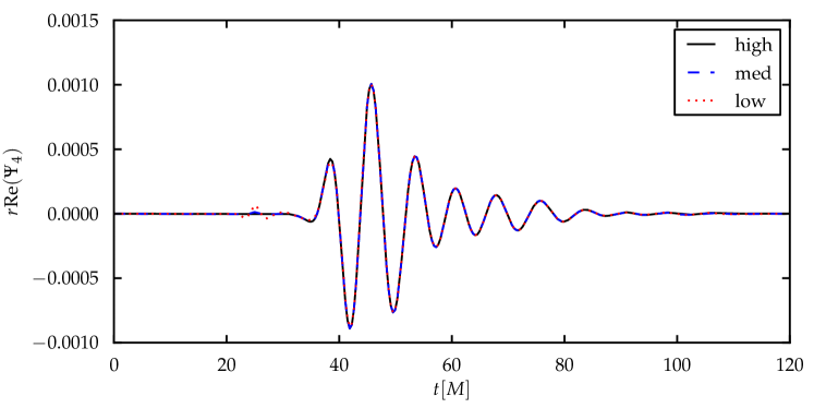
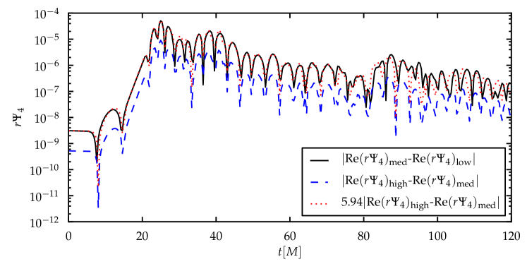
The top plot in this case shows only the real part of the extracted waveform but for all three resolutions (black solid curve is high, blue dashed curve is medium and red dotted curve is low resolution). Since the amplitude of this mode is almost a factor of 20 smaller than the mode there are actually small differences visible between resolutions in the beginning of the waveform. The bottom plot shows the convergence of the real part of the mode (compare with the bottom plot in Figure 9) and demonstrates that even though the amplitude is much smaller we still obtain close to perfect fourth-order convergence.
In addition to the modes shown in Figure 9 and 10 we note that the extracted mode is non-zero due to truncation error, but shows fourth-order convergence to zero with resolution (this mode is not present in the initial data and is not excited during the evolution). Other modes are zero to round-off due to symmetries at all resolutions.
Since there is non-trivial gravitational wave content in the initial data, the mass of the BH changes during its evolution. In figure 11, we show in the top plot the irreducible mass as calculated by AHFinderDirect as a function of time at the high (black solid curve), medium (blue dashed curve) and low (red dotted curve) resolutions.
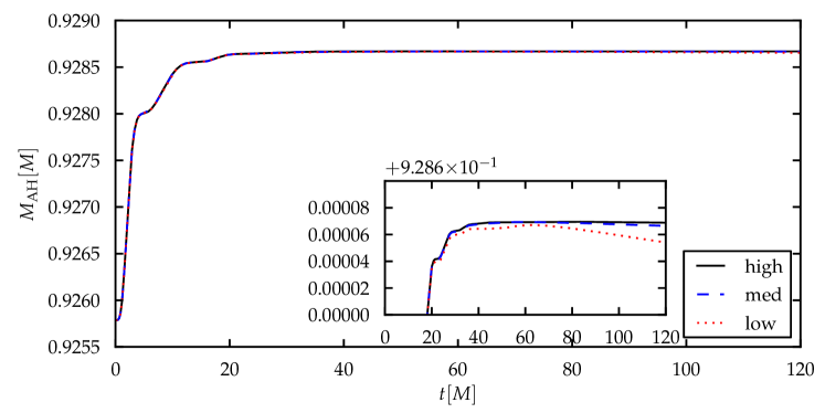
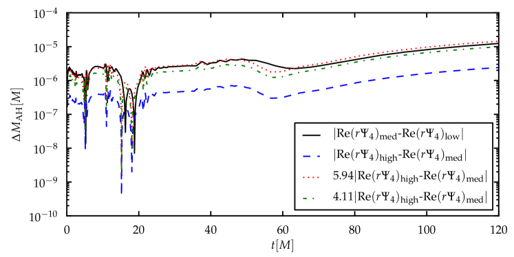
The inset shows in more detail the differences between the different resolutions. The irreducible mass increases by about 0.3% during the first of evolution and then remains constant (within numerical error) for the remainder of the evolution. The bottom plot shows the convergence of the irreducible mass by the difference between the medium and low resolutions (black solid curve), the difference between the high and medium resolutions (blue dashed curved) as well as the scaled difference between the high and medium resolutions for fourth-order (red dotted curve) and third-order (green dash-dotted curve). The convergence is almost perfectly fourth-order until , then better than fourth-order until , and finally between third-order and fourth-order for the remainder of the evolution. The lack of perfect fourth-order convergence at late times may be attributed to non-convergent errors from the puncture propagating to the horizon location at the lowest resolution.
Finally, in Figure 12 we show the total mass (top plot) and the change in the spin, , as calculated by QuasiLocalMeasures.
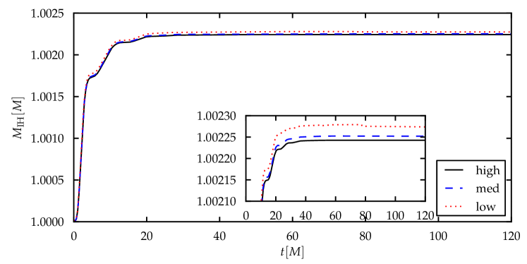
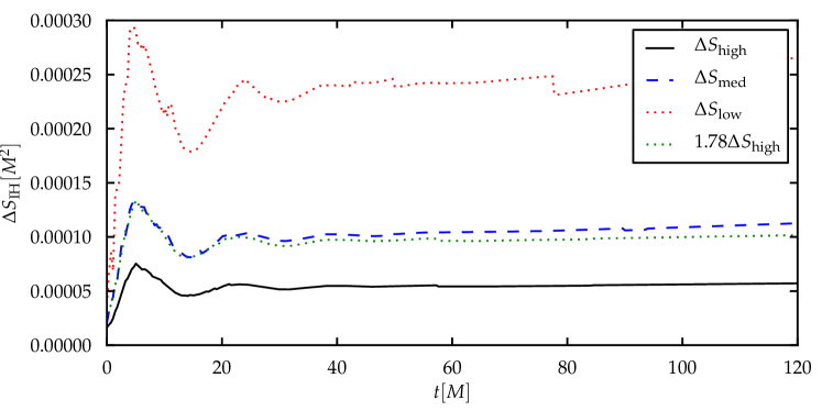
In both cases the black (solid) curve is for high, blue (dashed) for medium and red (dotted) for low resolution. Since the spacetime is axisymmetric the gravitational waves cannot radiate angular momentum. Thus any change in the spin must be due to numerical error and should converge to zero with increasing resolution. This is clearly shown in the bottom plot of Figure 12; the green (dash-dotted) curve (the high resolution result scaled by a factor of for second-order convergence to the resolution of the medium resolution) and the blue (dashed) curve are on top of each other. Since the QuasiLocalMeasures thorn uses an algorithm which is only second-order accurate overall, this is the expected result. The increase of about 0.22% in the mass of the BH is caused solely by the increase in the irreducible mass.
6.2 BH Binary
To demonstrate the performance in the code for a current problem of wide scientific interest, we have evolved a non-spinning equal-mass BH binary system. The initial data represent a binary system in a quasi-circular orbit, with an initial separation chosen to be so we may track the later inspiral, plunge, merger and ring down phases of the binary evolution. Table 1 provides more details about the initial binary parameters used to generate the initial data. The TwoPunctures module uses these initial parameters to solve (10), the elliptic Hamiltonian constraint for the regular component of the conformal factor (see section 5.2.3). The spectral solution for this example was determined by using collocation points, and, along with the Bowen-York analytic solution for the momentum constraints, represents constrained GR initial data . The evolution is performed by the McLachlan module.
| Configuration | ||||||
|---|---|---|---|---|---|---|
| QC3 | 3.0 | -3.0 | 0.0 | 0.13808 | 0.47656 | 0.984618 |
The simulation domain spans the coordinate range , where we have taken advantage of both the equatorial symmetry (implemented by the ReflectionSymmetry module) and the rotational symmetry around the -axis, which we apply at the plane using the RotatingSymmetry180 module. Carpet provides a hierarchy of refined grids centered at each puncture. Here, we used levels of refinement, where the box edge coordinate lengths are given by in units of the total binary mass, which is set to unity. Note that overlapping boxes are automatically redefined by Carpet into one unique region before the domain decomposition takes place.
Figure 13 shows the two puncture tracks throughout all phases of the binary evolution, provided by the PunctureTracker module. In the same plot we have recorded the intersection of the apparent horizon -surface with the plane every time interval during the evolution. A common horizon is first observed at . These apparent horizons were found by the AHFinderDirect module and their radius and location information stored as a -surface with spherical topology by the SphericalSurface module. The irreducible mass and dimensionless spin of the merged BH were calculated by the QuasiLocalMeasures module, and were found to be and , respectively.
Two modules are necessary to perform the waveform extraction. The first one, WeylScal4, calculates the Weyl scalar in term of the metric components and its derivatives; these were computed to be -th order accurate in this example. The second module, Multipole, interpolates the Weyl scalars onto spheres with centers and radii specified by the user, and performs a spherical harmonic multipole mode decomposition. Figure 13 shows the real and imaginary parts of the (, ) mode for extracted on a sphere centered at the origin at . The number of grid points on the sphere was set to be , which yields an angular resolution of radians, and an error of the same order, since the surface integrals were calculated by midpoint rule – a first order accurate method.
In order to evaluate the convergence of the numerical solution, we ran five simulations with different resolutions, and focus our analysis on the convergence of the phase and amplitude of the Weyl scalar . The mesh spacings adopted for the coarser grid in the AMR hierarchy for these different runs were , respectively, while the finer grid spacings can be easily found by dividing them by for the th level of mesh refinement.For this example, we set for the finest grid in the different AMR hierarchies, respectively.
Here, we consider the phase and the amplitude of the Weyl scalar at . In order to take differences between the numerical values at two different grid resolutions, we use an -th order accurate Lagrange operator to interpolate the higher-accuracy finite difference solution into the immediately coarser grid. We have experimented with -th and -th order as well, to evaluate the level of noise these interpolations could potentially introduce, but did not observe any noticeable difference and we report here on results from the higher-order option.
In Figure 14, we show the convergence of the amplitude and phase of the Weyl scalar by plotting the logarithm of the absolute value of the differences between two levels of resolution. The differences clearly converge to zero as the resolution is increased. We also indicate on both plots the time at which the gravitational wave frequency reaches . We follow a community standard, agreed to over the course of the NRAR[176] collaboration, that constrains the numerical resolution so that the accumulated phase error is not larger than radians at a gravitational wave frequency of . From the plot, we assert that the phase error between the higher and high resolutions and the one between high and medium-high resolutions satisfies this criterion, while the phase error between the medium-high and medium resolutions barely satisfies the criterion; and the one between medium and low resolutions does not. We conclude then that the three highest resolution runs do have sufficient resolution to extract waveforms for use in the construction of analytic waveform templates.
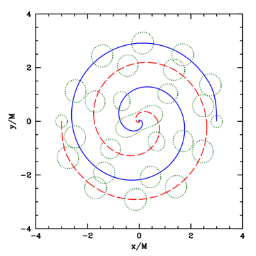
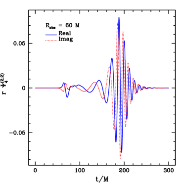
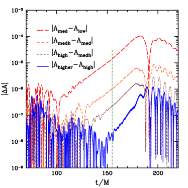
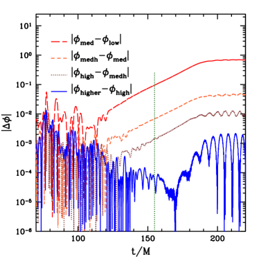
6.3 Linear oscillations of TOV stars
The examples in the previous subsections did not include the evolution of matter within a relativistic spacetime. One interesting test of a coupled matter-spacetime evolution is to measure the eigenfrequencies of a stable TOV star (see, e.g., [177, 178, 179, 180, 181]). These eigenfrequencies can be compared to values known from linear perturbation theory.
We begin our simulations with a self-gravitating fluid sphere, described by a polytropic equation of state. This one-dimensional solution is obtained by the code described in section 5.2.5, and is interpolated on the three-dimensional, computational evolution grid. This system is then evolved using the BSSN evolution system implemented in McLachlan and the hydrodynamics evolution system implemented in GRHydro.
For the test described here, we set up a stable TOV star described by a polytropic equation of state with and , and an initial central density of . This model can be taken to represent a non-rotating NS with a mass of . The computational domain is a cube of length with a base resolution of (, ) in each dimension. Four additional grids refine the region around the star centered at the origin, each doubling the resolution, with sizes of , , and , resulting in a resolution of (, ) across the entire star.
In Figure 15 we show the evolution of the central density of the star over an evolution time of (). The initial spike is due to the perturbation of the solution resulting from the interpolation onto the evolution grid. The remaining oscillations are mainly due to the interaction of the star and the artificial atmosphere and are present during the whole evolution. Given enough evolution time, the frequencies of these oscillations can be measured with satisfactory accuracy.
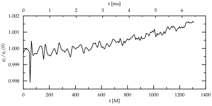
In Figure 16 we show the power spectral density (PSD) of the central density oscillations computed from a full 3D relativistic hydrodynamics simulation, compared to the corresponding frequencies as obtained with perturbative techniques (kindly provided by Kentaro Takami and computed using the method described in [182]). The PSD was computed using the entire time series of the high-resolution run, by removing the linear trend and averaging over Hanning windows overlapping half the signal length after padding the signal to five times its length. The agreement of the fundamental mode and first three overtone frequencies is clearly visible, but are limited beyond this by the finite numerical resolution. Higher overtones should be measurable with higher resolution, but at substantial computational cost.
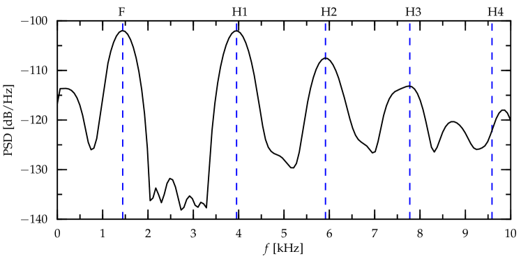
Within this test it is also interesting to study the convergence behavior of the coupled curvature and matter evolution code. One of the variables often used for this test is the Hamiltonian constraint violation. This violation vanishes for the continuum problem, but is non-zero and resolution-dependent in discrete simulations. The expected rate of convergence of the hydrodynamics code lies between and . It cannot be higher than due to the directional flux-split algorithm which is of second order. Depending on solution itself, the hydrodynamics code is only of first order in particular regions, e.g., at extrema (like the center of the star), or at the stellar surface.
Figure 17 shows the order of convergence of the Hamiltonian constraint violation, using the three highest-resolution runs, at the stellar center and a coordinate radius of which is about half way between the center and the surface. The observed convergence rate for most of the simulation time lies between and at the center, and between and at , consistent with the expected data-dependent convergence order of the underlying hydrodynamics evolution scheme.
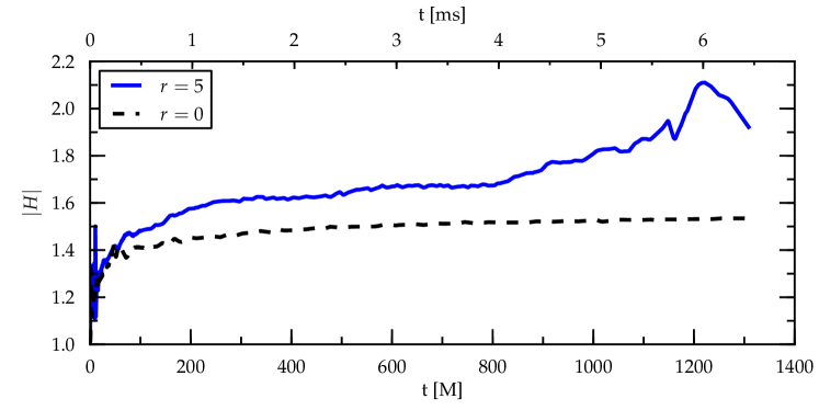
6.4 Neutron star collapse
The previous examples dealt either with preexisting BHs, either single or in a binary, or with a smooth singularity free spacetime, as in the case of the TOV star. The evolution codes in the toolkit are, however, also able to handle the dynamic formation of a singularity, that is follow a neutron star collapse into a BH. As a simple example of this process, we study the collapse of a non-rotating TOV star. We create initial data as in section 6.3 using and , , yielding a star model of gravitational mass , that is at the onset of instability. As is common in such situations (e.g., [95]), we trigger collapse by reducing the pressure support after the initial data have been constructed by lowering the polytropic constant from its initial value to . To ensure that the pressure-depleted configuration remains a solution of the Einstein constraint equations (91) in the presence of matter, we rescale the rest mass density such that the total energy density does not change:
| (93) |
Compared to the initial configuration, this rescaled star possesses a slightly higher central density and lower pressure. This change in accelerates the onset of collapse that would otherwise rely on being triggered by numerical noise, which would not be guaranteed to converge to a unique solution with increasing resolution. In order to resolve the star as well as to push the outer boundary far enough away (so that the star and the numerical outer boundary are not in causal contact during the simulation) we employ a fixed mesh refinement scheme. The outermost box has a radius of and a resolution of (, , for higher convergence levels). Around the star, centered about the origin, we stack extra boxes of approximate size for , where the resolution on each level is twice that of the surrounding level. In order to resolve the large density gradients developing during the collapse, two more levels with radii and are placed inside the star. We use the PPM reconstruction method and the HLLE Riemann solver to obtain second-order convergent results in smooth regions. Due to the presence of the density maximum at the center of the star and the non-smooth atmosphere at the edge of the star, we expect the observed convergence rate to be somewhat lower than second order, but higher than first order.
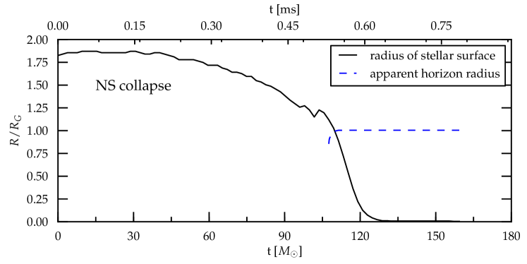
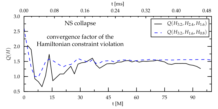
In Figure 18, we plot the approximate coordinate size of the star as well as the circumferential radius of the apparent horizon that eventually forms in the simulation. The apparent horizon is first found at approximately the time when the star’s coordinate radius approaches its Schwarzschild radius, though one needs to keep in mind that the Schwarzschild radius is a circumferential radius, whereas the meaning of the coordinate radius in our BSSN calculation is likely somewhat different. In Figure 19, we display the convergence factor obtained from
| (94) |
for the Hamiltonian constraint violation at the center of the collapsing star. Here is the Hamiltonian constraint violation (91) at the center of the star for a run with resolution . Up to the time when the apparent horizon forms, the convergence order is an expected . At later times, the singularity forming at the center of the collapsing star renders a pointwise measurement of the convergence factor at the center impossible.
6.5 Cosmology
The Einstein Toolkit is not only designed to evolve compact-object spacetimes, but also to solve the initial-value problem for spacetimes with radically different topologies and global properties. In this section, we illustrate the evolution of an initial-data set representing a constant- section of a spacetime from the Gowdy class [183, 184]. Models in this class have the line element:
| (95) |
defined on a 3-torus , , , with the functions , and to be determined by the Einstein equations. For , a coordinate transformation (plus a rescaling of the spatial coordinates) casts the line element into the form:
| (96) |
which represents the familiar Kasner spacetime for a homogeneous but anisotropically expanding universe. In the 3+1 decomposition described above, this reads:
| (97) | |||||
| (98) | |||||
| (99) | |||||
| (100) |
In Figure 20, we show the full evolution of the slice of spacetime (96), along with the associated error for a sequence of time resolutions.
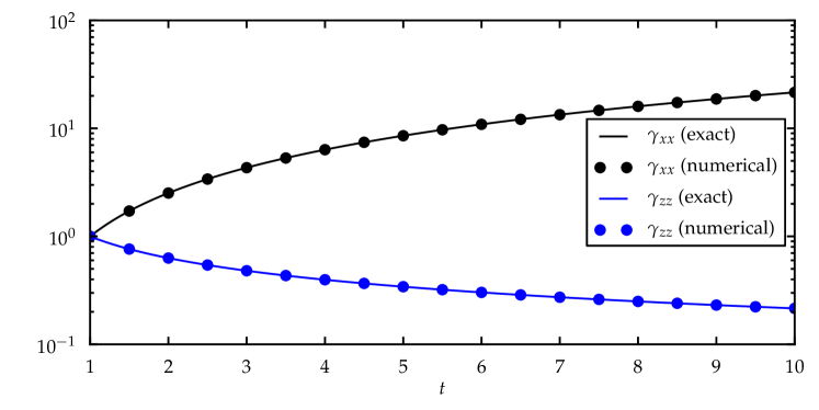
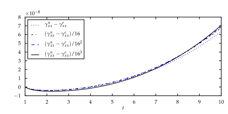
7 Conclusion and Future Work
In this article, we described the Einstein Toolkit, a collection of freely available and easy-to-use computational codes for numerical relativity and relativistic astrophysics. The code details and example results present in this article represent the state of the Einstein Toolkit in its release ET_2011_05 “Curie,” released on April 21, 2011.
The work presented here is but a snapshot of the Einstein Toolkit’s ongoing development, whose ultimate goal it is to provide an open-source set of robust baseline codes to realistically and reproducibly model the whole spectrum of relativistic astrophysical phenomena including, but not limited to, isolated black holes and neutron stars, binary black hole coalescence in vacuum and gaseous environments, double neutron star and neutron star – black hole mergers, core-collapse supernovae, and gamma-ray bursts.
For this, much future work towards including proper treatments of magnetic fields, more complex equations of state, nuclear reactions, neutrinos, and photons will be necessary and will need to be matched by improvements in infrastructure (e.g., more flexible AMR on general grids) and computing hardware for the required fully coupled 3-D, multi-scale, multi-physics simulations to become reality. These tasks, as well as the others mentioned below, are likely to occupy a great deal of the effort spent developing future versions of the Einstein Toolkit over the next few years.
Without a doubt, collapsing stars and merging BH-NS and NS-NS binaries must be simulated with GRMHD to capture the effects of magnetic fields that in many cases will alter the simulation outcome on a qualitative level and may be the driving mechanisms behind much of the observable EM signature from GRBs (e.g., [185]) and magneto-rotationally exploding core-collapse supernovae (e.g., [186]). To date, all simulations that have taken magnetic fields into account are still limited to the ideal MHD approximation, which assumes perfect conductivity. Non-ideal GRMHD schemes are just becoming available (see, e.g., [187, 188]), but have yet to be implemented widely in many branches of numerical relativity.
Most presently published 3D GR(M)HD simulations, with the exception of recent work on massive star collapse (see, e.g., [87]) and binary mergers (see, e.g., [48]), relied on simple zero-temperature descriptions of NS stellar structure, with many assuming simple polytropic forms. Such EOSs are computationally efficient, but are not necessarily a good description for matter in relativistic astrophysical systems. The inclusion of finite-temperature EOSs, derived from the microphysical descriptions of high-density matter, will lead to qualitatively different and much more astrophysically reliable results (see, e.g., [87]). In addition, most GR(M)HD studies neglect transport of neutrinos and photons and their interactions with matter. Neutrinos in particular play a crucial role in core-collapse supernovae and in the cooling of NS-NS merger remnants, thus they must not be left out when attempting to accurately model such events. Few studies have incorporated neutrino and/or photon transport and interactions in approximate ways (see, e.g., [87, 189, 48, 66]).
Besides new additions of physics modules, existing techniques require improvement. One example is the need for the gauge invariant extraction of gravitational waves from simulation spacetimes as realized by the Cauchy Characteristic Extraction (CCE) technique recently studied in [190, 112, 191]. The authors of one such CCE code [190] have agreed to make their work available to the whole community by integrating their CCE routines into the Einstein Toolkit release 2011_11 “Maxwell,” which will be described elsewhere.
A second much needed improvement of our existing methods is a transition to cell-centered AMR for GR hydrodynamic simulations, which would allow for exact flux conservation across AMR interfaces via a refluxing step that adjusts coarse and/or fine grid fluxes for consistency (e.g., [111]). This is also a prerequisite for the constrained transport method [192] for ensuring the divergence-free condition for the magnetic field in a future implementation of GRMHD within the Einstein Toolkit. Work towards cell-centered AMR, refluxing, and GRMHD is underway and will be reported in a future publication.
While AMR can increase resolution near regions of interest within the computational domain, it does not increase the convergence order of the underlying numerical methods. Simulations of BHs can easily make use of high-order numerical methods, with eighth-order convergence common at present. However, most GRMHD schemes, though they implement high-resolution shock-capturing methods, are limited to 2nd-order numerical accuracy in the hydrodynamic/MHD sector while performing curvature evolution with 4th-order accuracy or more. Higher order GRMHD schemes are used in fixed-background simulations (e.g., [193]), but still await implementation in fully dynamical simulations.
Yet another important goal is to increase the scalability of the Carpet AMR infrastructure. As we have shown, good scaling is limited to only a few thousand processes for some of the most widely used simulation scenarios. Work is in progress to eliminate this bottleneck [194]. On the other hand, a production simulation is typically composed of a large number of components, and even analysis and I/O routines have to scale well to achieve overall good performance. This is a highly non-trivial problem, since most Einstein Toolkit physics module authors are neither computer scientists nor have they had extensive training in parallel development and profiling techniques. Close collaboration with experts in these topics has been fruitful in the past and will be absolutely necessary for the optimization of Einstein Toolkit codes for execution on the upcoming generation of true petascale supercomputers on which typical compute jobs are expected to be running on 100,000 and more compute cores.
Acknowledgments
The authors wish to thank Ed Seidel whose inspiration and vision has driven work towards the Einstein Toolkit over the past 15 years. We are also grateful to the large number of people who contributed to the Einstein Toolkit via ideas, code, documentation, and testing; without these contributions, this toolkit would not exist today.
The Einstein Toolkit is directly supported by the National Science Foundation in the USA under the grant numbers 0903973/0903782/0904015 (CIGR). Related grants contribute directly and indirectly to the success of CIGR, including NSF OCI-0721915, NSF OCI-0725070, NSF OCI-0832606, NSF OCI-0905046, NSF OCI-0941653, NSF AST-0855535, NSF DMS-0820923, NASA 08-ATFP08-0093, EC-FP7 PIRG05-GA-2009-249290 and Deutsche Forschungsgemeinschaft grant SFB/Transregio 7 “Gravitational-Wave Astronomy”. Results presented in this article were obtained through computations on the Louisiana Optical Network Initiative under allocation loni_cactus05 and loni_numrel07, as well as on NSF XSEDE under allocations TG-MCA02N014, TG-PHY060027N, TG-PHY100033, at the National Energy Research Scientific Computing Center (NERSC), which is supported by the Office of Science of the US Department of Energy under contract DE-AC03-76SF00098, at the Leibniz Rechenzentrum of the Max Planck Society, and on Compute Canada resources via project cfz-411-aa.
G. Allen acknowledges that this material is based upon work supported while serving at the National Science Foundation. Any opinion, findings, and conclusions or recommendations expressed in this material are those of the authors and do not necessarily reflect the views of the National Science Foundation.
References
- [1] Shibata M and Uryu K 2000 Simulation of merging binary neutron stars in full general relativity: Gamma = two case Phys. Rev. D 61 064001
- [2] Shibata M and Uryu K 2002 Gravitational waves from the merger of binary neutron stars in a fully general relativistic simulation Prog. Theor. Phys. 107 265
- [3] Shibata M, Taniguchi K and Uryu K 2003 Merger of binary neutron stars of unequal mass in full general relativity Phys. Rev. D 68 084020
- [4] Shibata M, Taniguchi K and Uryu K 2005 Merger of binary neutron stars with realistic equations of state in full general relativity Phys. Rev. D 71 084021
- [5] Shibata M and Taniguchi K 2006 Merger of binary neutron stars to a black hole: disk mass, short gamma-ray bursts, and quasinormal mode ringing Phys. Rev. D 73 064027
- [6] Pretorius F 2005 Evolution of binary black hole spacetimes Phys. Rev. Lett. 95 121101
- [7] Campanelli M, Lousto C O, Marronetti P and Zlochower Y 2006 Accurate evolutions of orbiting black-hole binaries without excision Phys. Rev. Lett. 96 111101
- [8] Baker J G, Centrella J, Choi D I, Koppitz M and van Meter J 2006 Gravitational wave extraction from an inspiraling configuration of merging black holes Phys. Rev. Lett. 96 111102
- [9] Shibata M and Nakamura T 1995 Evolution of three-dimensional gravitational waves: Harmonic slicing case Phys. Rev. D 52 5428–5444
- [10] Baumgarte T W and Shapiro S L 1999 On the numerical integration of Einstein’s field equations Phys. Rev. D 59 024007
- [11] Baker J G, Centrella J, Choi D I, Koppitz M, van Meter J R and Miller M C 2006 Getting a kick out of numerical relativity Astrophys. J. 653 L93–L96
- [12] Campanelli M, Lousto C O, Zlochower Y and Merritt D 2007 Large merger recoils and spin flips from generic black-hole binaries Astrophys. J. 659 L5–L8
- [13] Holley-Bockelmann K, Gultekin K, Shoemaker D and Yunes N 2008 Gravitational Wave Recoil and the Retention of Intermediate Mass Black Holes Astrophys. J. 686 829–837
- [14] Pollney D, Reisswig C, Rezzolla L, Szilágyi B, Ansorg M, Deris B, Diener P, Dorband E N, Koppitz M, Nagar A and Schnetter E 2007 Recoil velocities from equal-mass binary black-hole mergers: a systematic investigation of spin-orbit aligned configurations Phys. Rev. D 76 124002
- [15] Lousto C O and Zlochower Y 2008 Further insight into gravitational recoil Phys. Rev. D 77 044028
- [16] Lousto C O and Zlochower Y 2009 Modeling gravitational recoil from precessing highly- spinning unequal-mass black-hole binaries Phys. Rev. D 79 064018
- [17] Baker J G, van Meter J R, McWilliams S T, Centrella J and Kelly B J 2007 Consistency of post-Newtonian waveforms with numerical relativity Phys. Rev. Lett. 99 181101
- [18] Husa S, Hannam M, Gonzalez J A, Sperhake U and Brügmann B 2008 Reducing eccentricity in black-hole binary evolutions with initial parameters from post-Newtonian inspiral Phys. Rev. D 77 044037
- [19] Baumgarte T, Brady P, Creighton J D E, Lehner L, Pretorius F and DeVoe R 2008 Learning about compact binary merger: The interplay between numerical relativity and gravitational-wave astronomy Phys. Rev. D 77 084009
- [20] Buonanno A, Cook G B and Pretorius F 2007 Inspiral, merger and ring-down of equal-mass black-hole binaries Phys. Rev. D 75 124018
- [21] Hannam M, Husa S, Brügmann B and Gopakumar A 2008 Comparison between numerical-relativity and post-Newtonian waveforms from spinning binaries: the orbital hang-up case Phys. Rev. D 78 104007
- [22] Gopakumar A, Hannam M, Husa S and Brügmann B 2008 Comparison between numerical relativity and a new class of post-Newtonian gravitational-wave phase evolutions: the non-spinning equal-mass case Phys. Rev. D 78 064026
- [23] Campanelli M, Lousto C O, Nakano H and Zlochower Y 2009 Comparison of Numerical and Post-Newtonian Waveforms for Generic Precessing Black-Hole Binaries Phys. Rev. D 79 084010
- [24] Buonanno A, Pan Y, Baker J G, Centrella J, Kelly B J, McWilliams S T and van Meter J R 2007 Towards faithful templates for non-spinning binary black holes using the effective-one-body approach Phys. Rev. D 76 104049
- [25] Ajith P, Babak S, Chen Y, Hewitson M, Krishnan B, Sintes A M, Whelan J T, Brügmann B, Diener P, Dorband E N, González J, Hannam M, Husa S, Pollney D, Rezzolla L, Santamaría L, Sperhake U and Thornburg J 2008 A Template bank for gravitational waveforms from coalescing binary black holes. I. Non-spinning binaries Phys. Rev. D 77 104017
- [26] Baker J G, Centrella J, Choi D I, Koppitz M and van Meter J 2006 Binary black hole merger dynamics and waveforms Phys. Rev. D 73 104002
- [27] Baker J G, Campanelli M, Pretorius F and Zlochower Y 2007 Comparisons of binary black hole merger waveforms Class. Quantum Grav. 24 S25–S31
- [28] Campanelli M, Lousto C O and Zlochower Y 2006 Gravitational radiation from spinning-black-hole binaries: The orbital hang up Phys. Rev. D 74 041501
- [29] Campanelli M, Lousto C O and Zlochower Y 2006 Spin-orbit interactions in black-hole binaries Phys. Rev. D 74 084023
- [30] Campanelli M, Lousto C O, Zlochower Y, Krishnan B and Merritt D 2007 Spin Flips and Precession in Black-Hole-Binary Mergers Phys. Rev. D 75 064030
- [31] Herrmann F, Hinder I, Shoemaker D M, Laguna P and Matzner R A 2007 Binary Black Holes: Spin Dynamics and Gravitational Recoil Phys. Rev. D 76 084032
- [32] Rezzolla L, Barausse E, Dorband E N, Pollney D, Reisswig C, Seiler J and Husa S 2008 On the final spin from the coalescence of two black holes Phys. Rev. D 78 044002
- [33] Berti E, Cardoso V, Gonzalez J A, Sperhake U and Brügmann B 2008 Multipolar analysis of spinning binaries Class. Quantum Grav. 25 114035
- [34] Pretorius F and Khurana D 2007 Black hole mergers and unstable circular orbits Class. Quantum Grav. 24 S83–S108
- [35] Sperhake U, Berti E, Cardoso V, González J A, Brügmann B and Ansorg M 2008 Eccentric binary black-hole mergers: The transition from inspiral to plunge in general relativity Phys. Rev. D 78 064069
- [36] Hinder I, Vaishnav B, Herrmann F, Shoemaker D and Laguna P 2008 Universality and Final Spin in Eccentric Binary Black Hole Inspirals Phys. Rev. D 77 081502
- [37] Grigsby J D and Cook G B 2008 Measuring eccentricity in binary black-hole initial data Phys. Rev. D 77 044011
- [38] Pfeiffer H P, Brown D A, Kidder L E, Lindblom L, Lovelace G and Scheel M A 2007 Reducing orbital eccentricity in binary black hole simulations Class. Quantum Grav. 24 S59–S82
- [39] Stephens B C, East W E and Pretorius F 2011 Eccentric Black Hole-Neutron Star Mergers Astrophys. J. 737 L5
- [40] Font J A 2008 Numerical hydrodynamics and magnetohydrodynamics in general relativity Living Reviews in Relativity 11 7
- [41] Hawley J F 2009 MHD simulations of accretion disks and jets: strengths and limitations Astrophys. Space. Sci. 320 107–114
- [42] Pandharipande V R and Ravenhall D G 1989 Hot Nuclear Matter NATO ASIB Proc. 205: Nuclear Matter and Heavy Ion Collisions ed M Soyeur, H Flocard, B Tamain, & M Porneuf pp 103–132
- [43] Douchin F and Haensel P 2001 A unified equation of state of dense matter and neutron star structure Astron. Astrophys. 380 151–167
- [44] Akmal A, Pandharipande V and Ravenhall D 1998 The Equation of state of nucleon matter and neutron star structure Phys. Rev. C 58 1804–1828
- [45] Shen H, Toki H, Oyamatsu K and Sumiyoshi K 1998 Relativistic equation of state of nuclear matter for supernova explosion Prog. Theor. Phys. 100 1013
- [46] Shen H, Toki H, Oyamatsu K and Sumiyoshi K 1998 Relativistic equation of state of nuclear matter for supernova and neutron star Nucl. Phys. A 637 435–450
- [47] Lattimer J M and Swesty F D 1991 A Generalized equation of state for hot, dense matter Nucl. Phys. A 535 331–376
- [48] Sekiguchi Y, Kiuchi K, Kyutoku K and Shibata M 2011 Gravitational waves and neutrino emission from the merger of binary neutron stars Phys. Rev. Lett. 107 051102
- [49] O’Connor E and Ott C D 2010 A New Open-Source Code for Spherically-Symmetric Stellar Collapse to Neutron Stars and Black Holes Class. Quant. Grav. 27 114103
- [50] Anderson M, Hirschmann E W, Lehner L, Liebling S L, Motl P M et al. 2008 Simulating binary neutron stars: Dynamics and gravitational waves Phys. Rev. D 77 024006
- [51] Anderson M, Hirschmann E W, Lehner L, Liebling S L, Motl P M et al. 2008 Magnetized Neutron Star Mergers and Gravitational Wave Signals Phys. Rev. Lett. 100 191101
- [52] Baiotti L, Giacomazzo B and Rezzolla L 2008 Accurate evolutions of inspiralling neutron-star binaries: prompt and delayed collapse to black hole Phys. Rev. D 78 084033
- [53] Baiotti L, Giacomazzo B and Rezzolla L 2009 Accurate evolutions of inspiralling neutron-star binaries: assessment of the truncation error Class. Quantum Grav. 26 114005
- [54] Baiotti L, Damour T, Giacomazzo B, Nagar A and Rezzolla L 2010 Analytic modelling of tidal effects in the relativistic inspiral of binary neutron stars Phys. Rev. Lett. 105 261101
- [55] Baiotti L, Damour T, Giacomazzo B, Nagar A and Rezzolla L 2011 Accurate numerical simulations of inspiralling binary neutron stars and their comparison with effective-one-body analytical models Phys. Rev. D 84 024017
- [56] Bernuzzi S, Thierfelder M and Bruegmann B 2011 Accuracy of numerical relativity waveforms from binary neutron star mergers and their comparison with post-Newtonian waveforms (Preprint arXiv:1109.3611)
- [57] Giacomazzo B, Rezzolla L and Baiotti L 2009 Can magnetic fields be detected during the inspiral of binary neutron stars? Mon. Not. Roy. Astron. Soc. 399 L164–L168
- [58] Giacomazzo B, Rezzolla L and Baiotti L 2011 Accurate evolutions of inspiralling and magnetized neutron-stars: Equal-mass binaries Phys. Rev. D 83 044014
- [59] Gold R, Bernuzzi S, Thierfelder M, Bruegmann B and Pretorius F 2011 Eccentric binary neutron star mergers (Preprint arXiv:1109.5128)
- [60] Hotokezaka K, Kyutoku K, Okawa H, Shibata M and Kiuchi K 2011 Binary Neutron Star Mergers: Dependence on the Nuclear Equation of State Phys. Rev. D 83 124008
- [61] Kiuchi K, Sekiguchi Y, Shibata M and Taniguchi K 2009 Longterm general relativistic simulation of binary neutron stars collapsing to a black hole Phys. Rev. D 80 064037
- [62] Kiuchi K, Sekiguchi Y, Shibata M and Taniguchi K 2010 Exploring binary-neutron-star-merger scenario of short-gamma-ray bursts by gravitational-wave observation Phys. Rev. Lett. 104 141101
- [63] Liu Y T, Shapiro S L, Etienne Z B and Taniguchi K 2008 General relativistic simulations of magnetized binary neutron star mergers Phys. Rev. D 78 024012
- [64] Rezzolla L, Baiotti L, Giacomazzo B, Link D and Font J A 2010 Accurate evolutions of unequal-mass neutron-star binaries: properties of the torus and short GRB engines Class. Quantum Grav. 27 114105
- [65] Rezzolla L, Giacomazzo B, Baiotti L, Granot J, Kouveliotou C and Aloy M A 2011 The missing link: Merging neutron stars naturally produce jet-like structures and can power short Gamma-Ray Bursts Astrophys. J. 732 L6
- [66] Sekiguchi Y, Kiuchi K, Kyutoku K and Shibata M 2011 Effects of hyperons in binary neutron star mergers (Preprint arXiv:1110.4442)
- [67] Thierfelder M, Bernuzzi S and Bruegmann B 2011 Numerical relativity simulations of binary neutron stars Phys. Rev. D 84 044012
- [68] Yamamoto T, Shibata M and Taniguchi K 2008 Simulating coalescing compact binaries by a new code SACRA Phys. Rev. D 78 064054
- [69] Chawla S, Anderson M, Besselman M, Lehner L, Liebling S L, Motl P M and Neilsen D 2010 Mergers of Magnetized Neutron Stars with Spinning Black Holes: Disruption, Accretion and Fallback Phys. Rev. Lett. 105 111101
- [70] Duez M D, Foucart F, Kidder L E, Pfeiffer H P, Scheel M A and Teukolsky S A 2008 Evolving black hole-neutron star binaries in general relativity using pseudospectral and finite difference methods Phys. Rev. D 78 104015
- [71] Duez M D, Foucart F, Kidder L E, Ott C D and Teukolsky S A 2010 Equation of state effects in black hole-neutron star mergers Class. Quantum Grav. 27 114106
- [72] Etienne Z B, Faber J A, Liu Y T, Shapiro S L, Taniguchi K and Baumgarte T W 2008 Fully General Relativistic Simulations of Black Hole- Neutron Star Mergers Phys. Rev. D 77 084002
- [73] Etienne Z B, Liu Y T, Shapiro S L and Baumgarte T W 2009 General relativistic simulations of black-hole-neutron-star mergers: Effects of black-hole spin Phys. Rev. D 79 044024
- [74] Foucart F, Duez M D, Kidder L E and Teukolsky S A 2011 Black hole-neutron star mergers: effects of the orientation of the black hole spin Phys. Rev. D 83 024005
- [75] Foucart F, Duez M D, Kidder L E, Scheel M A, Szilagyi B et al. 2011 Black hole-neutron star mergers for 10 solar mass black holes (Preprint arXiv:1111.1677)
- [76] Kyutoku K, Shibata M and Taniguchi K 2010 Gravitational waves from nonspinning black hole-neutron star binaries: dependence on equations of state Phys. Rev. D 82 044049
- [77] Kyutoku K, Okawa H, Shibata M and Taniguchi K 2011 Gravitational waves from spinning black hole-neutron star binaries: dependence on black hole spins and on neutron star equations of state Phys. Rev. D 84 064018
- [78] Lackey B D, Kyutoku K, Shibata M, Brady P R and Friedman J L 2011 Extracting equation of state parameters from black hole-neutron star mergers. I. Nonspinning black holes (Preprint arXiv:1109.3402)
- [79] Löffler F, Rezzolla L and Ansorg M 2006 Numerical evolutions of a black hole-neutron star system in full general relativity: Head-on collision Phys. Rev. D 74 104018
- [80] Shibata M and Uryu K 2007 Merger of black hole-neutron star binaries in full general relativity Class. Quantum Grav. 24 S125–S138
- [81] Shibata M and Uryu K 2006 Merger of black hole-neutron star binaries: Nonspinning black hole case Phys. Rev. D 74 121503
- [82] Shibata M and Taniguchi K 2008 Merger of black hole and neutron star in general relativity: Tidal disruption, torus mass, and gravitational waves Phys. Rev. D 77 084015
- [83] Shibata M, Kyutoku K, Yamamoto T and Taniguchi K 2009 Gravitational waves from black hole-neutron star binaries I: Classification of waveforms Phys. Rev. D 79 044030
- [84] Shibata M and Kyutoku K 2010 Constraining nuclear-matter equations of state by gravitational waves from black hole-neutron star binaries Prog. Theor. Phys. Suppl. 186 17–25
- [85] Faber J 2009 Status of neutron star-black hole and binary neutron star simulations Class. Quantum Grav. 26 114004
- [86] Duez M D 2010 Numerical relativity confronts compact neutron star binaries: a review and status report Class. Quantum Grav. 27 114002
- [87] Ott C D, Dimmelmeier H, Marek A, Janka H T, Hawke I, Zink B and Schnetter E 2007 3D Collapse of Rotating Stellar Iron Cores in General Relativity with Microphysics Phys. Rev. Lett. 98 261101
- [88] Ott C D, Dimmelmeier H, Marek A, Janka H T, Zink B, Hawke I and Schnetter E 2007 Rotating Collapse of Stellar Iron Cores in General Relativity Class. Quantum Grav. 24 S139–S154
- [89] Shibata M and Sekiguchi Y i 2005 Three-dimensional simulations of stellar core collapse in full general relativity: Nonaxisymmetric dynamical instabilities Phys. Rev. D 71 024014
- [90] Shibata M, Liu Y T, Shapiro S L and Stephens B C 2006 Magnetorotational collapse of massive stellar cores to neutron stars: Simulations in full general relativity Phys. Rev. D 74 104026
- [91] Shibata M, Baumgarte T W and Shapiro S L 2000 Stability and collapse of rapidly rotating, supramassive neutron stars: 3D simulations in general relativity Phys. Rev. D 61 044012
- [92] Duez M D, Liu Y T, Shapiro S L and Stephens B C 2005 Relativistic magnetohydrodynamics in dynamical spacetimes: Numerical methods and tests Phys. Rev. D 72 024028
- [93] Duez M D, Liu Y T, Shapiro S L, Shibata M and Stephens B C 2006 Collapse of magnetized hypermassive neutron stars in general relativity Phys. Rev. Lett. 96 031101
- [94] Baiotti L, Hawke I, Montero P J, Löffler F, Rezzolla L, Stergioulas N, Font J A and Seidel E 2005 Three-dimensional relativistic simulations of rotating neutron star collapse to a Kerr black hole Phys. Rev. D 71 024035
- [95] Baiotti L, Hawke I, Rezzolla L and Schnetter E 2005 Gravitational-wave emission from rotating gravitational collapse in three dimensions Phys. Rev. Lett. 94 131101
- [96] Baiotti L, De Pietri R, Manca G M and Rezzolla L 2007 Accurate simulations of the dynamical barmode instability in full General Relativity Phys. Rev. D 75 044023
- [97] Manca G M, Baiotti L, De Pietri R and Rezzolla L 2007 Dynamical non-axisymmetric instabilities in rotating relativistic stars Class. Quantum Grav. 24 S171–S186
- [98] Cactus Computational Toolkit URL http://www.cactuscode.org/
- [99] Djikstra F and van der Steen A J 2006 Integration of two ocean models within Cactus Concurrency and Computation: Practice and Experience 18 193–202
- [100] Camarda K, He Y and Bishop K 2001 A parallel chemical reaction simulation using cactus Linux Clusters: The HPC Revolution
- [101] Einstein Toolkit: Open software for relativistic astrophysics URL http://einsteintoolkit.org/
- [102] Goodale T, Allen G, Lanfermann G, Massó J, Radke T, Seidel E and Shalf J 2003 The Cactus framework and toolkit: Design and applications Vector and Parallel Processing – VECPAR’2002, 5th International Conference, Lecture Notes in Computer Science (Berlin: Springer) URL http://edoc.mpg.de/3341
- [103] Allen G, Goodale T, Lanfermann G, Radke T, Rideout D and Thornburg J 2011 Cactus Users’ Guide URL http://www.cactuscode.org/Guides/Stable/UsersGuide/UsersGuide%Stable.pdf
- [104] Anninos P et al. 1995 Three-dimensional numerical relativity: The Evolution of black holes Phys. Rev. D 52 2059–2082
- [105] Anninos P, Masso J, Seidel E, Suen W M and Tobias M 1997 Dynamics of gravitational waves in 3D: Formulations, methods, and tests Phys. Rev. D 56 842–858
- [106] Seidel E and Suen W M 1999 Numerical Relativity As A Tool For Computational Astrophysics J. Comput. Appl. Math 109 493–525
- [107] Cactus runs on 131,072 cores on Blue Gene/P at ANL URL http://cactuscode.org/media/news/BGP-131072/
- [108] Schnetter E, Hawley S H and Hawke I 2004 Evolutions in 3-D numerical relativity using fixed mesh refinement Class. Quantum Grav. 21 1465–1488
- [109] Schnetter E, Diener P, Dorband E N and Tiglio M 2006 A multi-block infrastructure for three-dimensional time-dependent numerical relativity Class. Quantum Grav. 23 S553–S578
- [110] Carpet: Adaptive Mesh Refinement for the Cactus Framework URL http://www.carpetcode.org/
- [111] Berger M J and Oliger J 1984 Adaptive Mesh Refinement for Hyperbolic Partial Differential Equations J. Comput. Phys. 53 484
- [112] Reisswig C, Ott C D, Sperhake U and Schnetter E 2011 Gravitational Wave Extraction in Simulations of Rotating Stellar Core Collapse Phys. Rev. D 83 064008
- [113] Lousto C O and Zlochower Y 2011 Orbital Evolution of Extreme-Mass-Ratio Black-Hole Binaries with Numerical Relativity Phys. Rev. Lett. 106 041101
- [114] Thomas M W and Schnetter E 2010 Simulation Factory: Taming application configuration and workflow on high-end resources (Preprint arXiv:1008.457)
- [115] SimFactory: Herding numerical simulations URL http://simfactory.org/
- [116] Husa S, Hinder I and Lechner C 2006 Kranc: a Mathematica application to generate numerical codes for tensorial evolution equations Comput. Phys. Commun. 174 983–1004
- [117] Lechner C, Alic D and Husa S 2004 From Tensor Equations to Numerical Code – Computer Algebra Tools for Numerical Relativity (Preprint arXiv:cs/0411063)
- [118] Kranc: Kranc assembles numerical code URL http://kranccode.org/
- [119] Pollney D, Reisswig C, Schnetter E, Dorband N and Diener P 2011 High accuracy binary black hole simulations with an extended wave zone Phys. Rev. D 83 044045
- [120] Alcubierre M 2008 Introduction to 3+1 Numerical Relativity (Oxford University Press)
- [121] Baumgarte T W and Shapiro S L 2010 Numerical Relativity: Solving Einstein’s Equations on the Computer (Cambridge University Press)
- [122] Centrella J, Baker J G, Kelly B J and van Meter J R 2010 Black-hole binaries, gravitational waves, and numerical relativity Rev. Mod. Phys. 82 3069–3119
- [123] Arnowitt R L, Deser S and Misner C W 2008 The dynamics of general relativity General Relativity and Gravitation 40 1997–2027
- [124] Martí J M, Ibáñez J M and Miralles J M 1991 Numerical relativistic hydrodynamics: Local characteristic approach Phys. Rev. D 43 3794–3801
- [125] Banyuls F, Font J A, Ibanez J M, Marti J M and Miralles J A 1997 Numerical 3+1 General Relativistic Hydrodynamics: A Local Characteristic Approach Astrophys. J. 476 221
- [126] Ibáñez J, Aloy M, Font J, Martí J, Miralles J and Pons J 2001 Riemann solvers in general relativistic hydrodynamics Proceedings of Godunov Methods, Theory and Applications 1999 ed Toro E (New York: Kluwer Academic/Plenum Publishers) p 485
- [127] Ansorg M, Brügmann B and Tichy W 2004 A single-domain spectral method for black hole puncture data Phys. Rev. D 70 064011
- [128] GSL: The GNU scientific library URL http://www.gnu.org/software/gsl/
- [129] Galassi M, Davies J, Theiler J, Gough B, Jungman G, Alken P, Booth M and Rossi F 2009 GNU Scientific Library Reference Manual 3rd ed (Network Theory Ltd.) ISBN 0-9546120-7-8
- [130] LORENE: Langage objet pour la relativite numerique URL http://www.lorene.obspm.fr/
- [131] Gourgoulhon E, Grandclement P, Taniguchi K, Marck J A and Bonazzola S 2001 Quasiequilibrium sequences of synchronized and irrotational binary neutron stars in general relativity. I. Method and tests Phys. Rev. D 63 064029
- [132] York Jr J W 1999 Conformal ’thin sandwich’ data for the initial-value problem of General Relativity Phys. Rev. Lett. 82 1350–1353
- [133] Brill D R 1959 On the positive definite mass of the Bondi-Weber-Wheeler time-symmetric gravitational waves Annals Phys. 7 466–483
- [134] Martí J M and Müller E 1999 Numerical hydrodynamics in special relativity Living Reviews in Relativity 2 3
- [135] Brandt S and Brügmann B 1997 Black hole punctures as initial data for general relativity Phys. Rev. Lett. 78 3606–3609
- [136] Bowen J M and York James W J 1980 Time asymmetric initial data for black holes and black hole collisions Phys. Rev. D 21 2047–2056
- [137] Grandclement P, Gourgoulhon E and Bonazzola S 2002 Binary black holes in circular orbits. II. Numerical methods and first results Phys. Rev. D 65 044021
- [138] Tolman R C 1939 Static solutions of Einstein’s field equations for spheres of fluid Phys. Rev. 55 364–373
- [139] Oppenheimer J R and Volkoff G M 1939 On Massive neutron cores Phys. Rev. 55 374–381
- [140] Brown J D, Diener P, Sarbach O, Schnetter E and Tiglio M 2009 Turduckening black holes: an analytical and computational study Phys. Rev. D 79 044023
- [141] York Jr J W 1979 Kinematics and dynamics of general relativity Sources of Gravitational Radiation ed L L Smarr pp 83–126
- [142] Alcubierre M, Brügmann B, Dramlitsch T, Font J A, Papadopoulos P, Seidel E, Stergioulas N and Takahashi R 2000 Towards a stable numerical evolution of strongly gravitating systems in general relativity: The Conformal treatments Phys. Rev. D 62 044034
- [143] Alcubierre M, Brügmann B, Diener P, Koppitz M, Pollney D, Seidel E and Takahashi R 2003 Gauge conditions for long term numerical black hole evolutions without excision Phys. Rev. D 67 084023
- [144] Muller D and Bruegmann B 2010 Toward a dynamical shift condition for unequal mass black hole binary simulations Class. Quant. Grav. 27 114008
- [145] Schnetter E 2010 Time Step Size Limitation Introduced by the BSSN Gamma Driver Class. Quantum Grav. 27 167001
- [146] Hawke I, Löffler F and Nerozzi A 2005 Excision methods for high resolution shock capturing schemes applied to general relativistic hydrodynamics Phys. Rev. D 71 104006
- [147] Baiotti L, Hawke I, Montero P J and Rezzolla L 2003 A new three-dimensional general-relativistic hydrodynamics code Mem. Soc. Ast. It. 74 S210
- [148] Whisky – relativistic hydrodynamics and magnetohydrodynamics URL http://www.whiskycode.org/
- [149] Hyman J M 1976 The method of lines solution of partial differential equations Tech. Rep. COO-3077-139 ERDA Mathematics and Computing Laboratory, Courant Institute of Mathematical Sciences, New York University
- [150] Roe P L 1986 Characteristic-based schemes for the Euler equations Ann. Rev. Fluid Mech. 18 337–365
- [151] van Leer B 1977 Towards the ultimate conservative difference scheme. III - Upstream-centered finite-difference schemes for ideal compressible flow. IV - A new approach to numerical convection J. Comp. Phys. 23 263–299
- [152] Colella P and Woodward P R 1984 The Piecewise Parabolic Method (PPM) for Gas Dynamical Simulations J. Comp. Phys. 54 174–201
- [153] Harten A, Engquist B, Osher S and Chakravarthy S R 1987 Uniformly High Order Accurate Essentially Non-oscillatory Schemes III Journal of Computational Physics 71 231–303
- [154] Shu C W 1999 High order methods for computational physics / ed Barth T J and Deconinck H A (New York: Springer) pp 439–582
- [155] Harten A, Lax P D and van Leer B 1983 On upstream differencing and godunov-type schemes for hyperbolic conservation laws SIAM review 25 35
- [156] Einfeldt B 1988 On Godunov-type methods for gas dynamics SIAM J. Numer. Anal. 25 294–318
- [157] Roe P L 1981 Approximate Riemann Solvers, Parameter Vectors, and Difference Schemes Journal of Computational Physics 43 357–372
- [158] Donat R and Marquina A 1996 Capturing Shock Reflections: An Improved Flux Formula Journal of Computational Physics 125 42–58
- [159] Aloy M, Ibanez J, Marti J and Muller E 1999 Genesis: a high resolution code for 3-D relativistic hydrodynamics Astrophys. J. Suppl. 122 151–166
- [160] Janka H T, Zwerger T and Moenchmeyer R 1993 Does artificial viscosity destroy prompt type-II supernova explosions? Astron. Astrophys. 268 360–368
- [161] Dimmelmeier H, Ott C D, Janka H T, Marek A and Mueller E 2007 Generic Gravitational Wave Signals from the Collapse of Rotating Stellar Cores Phys. Rev. Lett. 98 251101
- [162] Diener P 2003 A new general purpose event horizon finder for 3D numerical spacetimes Class. Quantum Grav. 20 4901–4918
- [163] Anninos P, Camarda K, Libson J, Mass’o J, Seidel E and Suen W M 1998 Finding apparent horizons in dynamic 3-d numerical space-times Phys. Rev. D 58 024003
- [164] Gundlach C 1998 Pseudospectral apparent horizon finders: An Efficient new algorithm Phys. Rev. D 57 863–875
- [165] Thornburg J 2004 A Fast Apparent-Horizon Finder for 3-Dimensional Cartesian Grids in Numerical Relativity Class. Quantum Grav. 21 743–766
- [166] McLachlan, a public BSSN code URL http://www.cct.lsu.edu/~eschnett/McLachlan/
- [167] Yo H J, Baumgarte T W and Shapiro S L 2002 Improved numerical stability of stationary black hole evolution calculations Phys. Rev. D 66 084026
- [168] Dreyer O, Krishnan B, Shoemaker D and Schnetter E 2003 Introduction to isolated horizons in numerical relativity Phys. Rev. D 67 024018
- [169] Schnetter E, Krishnan B and Beyer F 2006 Introduction to dynamical horizons in numerical relativity Phys. Rev. D 74 024028
- [170] Szabados L B 2004 Quasi-Local Energy-Momentum and Angular Momentum in GR: A Review Article Living Reviews in Relativity 7 4
- [171] Lovelace G, Chen Y, Cohen M, Kaplan J D, Keppel D et al. 2010 Momentum flow in black-hole binaries. II. Numerical simulations of equal-mass, head-on mergers with antiparallel spins Phys. Rev. D 82 064031
- [172] Moncrief V 1974 Gravitational perturbations of spherically symmetric systems. I. The exterior problem. Annals Phys. 88 323–342
- [173] Regge T and Wheeler J A 1957 Stability of a Schwarzschild singularity Phys. Rev. 108 1063–1069
- [174] Baker J G, Campanelli M and Lousto C O 2002 The Lazarus project: A Pragmatic approach to binary black hole evolutions Phys. Rev. D 65 044001
- [175] Alcubierre M, Brandt S, Brügmann B, Holz D, Seidel E, Takahashi R and Thornburg J 2001 Symmetry without Symmetry: Numerical Simulation of Axisymmetric Systems using Cartesian Grids Int. J. Mod. Phys. D 10 273–290
- [176] NRAR: Numerical-relativity and analytical-relativity collaboration URL https://www.ninja-project.org/doku.php?id=nrar:home
- [177] Gourgoulhon E 1991 Simple equations for general relativistic hydrodynamics in spherical symmetry applied to neutron star collapse Astron. Astrophys. 252 651–663
- [178] Romero J V, Ibanez J M A, Marti J M A and Miralles J A 1996 A New Spherically Symmetric General Relativistic Hydrodynamical Code Astrophys. J. 462 839–854
- [179] Shibata M, Baumgarte T W and Shapiro S L 1998 Stability of coalescing binary stars against gravitational collapse: Hydrodynamical simulations Phys. Rev. D 58 023002
- [180] Font J A, Goodale T, Iyer S, Miller M A, Rezzolla L, Seidel E, Stergioulas N, Suen W M and Tobias M 2002 Three-dimensional general relativistic hydrodynamics. 2. Long term dynamics of single relativistic stars Phys. Rev. D 65 084024
- [181] Shibata M 2003 Axisymmetric general relativistic hydrodynamics: Long term evolution of neutron stars and stellar collapse to neutron stars and black holes Phys. Rev. D 67 024033
- [182] Yoshida S and Eriguchi Y 2001 Quasiradial modes of rotating stars in general relativity Mon. Not. Roy. Astron. Soc. 322 389–396
- [183] Gowdy R 1971 Gravitational waves in closed universes Phys. Rev. Lett. 27 826–829
- [184] New K C, Watt K, Misner C W and Centrella J M 1998 Stable three level leapfrog integration in numerical relativity Phys. Rev. D 58 064022
- [185] Woosley S E and Bloom J S 2006 The Supernova – Gamma-Ray Burst Connection Ann. Rev. Astron. Astrophys. 44 507–556
- [186] Burrows A, Dessart L, Livne E, Ott C D and Murphy J 2007 Simulations of Magnetically-Driven Supernova and Hypernova Explosions in the Context of Rapid Rotation Astrophys. J. 664 416–434
- [187] Palenzuela C, Lehner L, Reula O and Rezzolla L 2009 Beyond ideal MHD: towards a more realistic modeling of relativistic astrophysical plasmas Mon. Not. Roy. Astron. Soc. 394 1727–1740
- [188] Del Zanna L, Zanotti O, Bucciantini N and Londrillo P 2007 ECHO: an Eulerian Conservative High Order scheme for general relativistic magnetohydrodynamics and magnetodynamics Astron. Astrophys. 473 11–30
- [189] Farris B D, Li T K, Liu Y T and Shapiro S L 2008 Relativistic Radiation Magnetohydrodynamics in Dynamical Spacetimes: Numerical Methods and Tests Phys. Rev. D 78 024023
- [190] Babiuc M C, Szilágyi B, Winicour J and Zlochower Y 2011 Characteristic extraction tool for gravitational waveforms Phys Rev. D. 84 044057
- [191] Reisswig C, Bishop N T, Pollney D and Szilágyi B 2010 Characteristic extraction in numerical relativity: binary black hole merger waveforms at null infinity Classical and Quantum Gravity 27 075014
- [192] Tóth G 2000 The Constraint in Shock-Capturing Magnetohydrodynamics Codes Journal of Computational Physics 161 605–652
- [193] Tchekhovskoy A, McKinney J C and Narayan R 2007 WHAM: A WENO-based general relativistic numerical scheme I: Hydrodynamics Mon. Not. Roy. Astron. Soc. 379 469–497
- [194] Zebrowski A, Löffler F and Schnetter E 2011 The BL-Octree: An Efficient Data Structure for Discretized Block-Based Adaptive Mesh Refinement ParCo2011: Proceeings of the 2011 International Conference on Parallel Computing (ParCo Conferences)