Semi-supervised deep learning for postmerger binary neutron star waveforms

Using machine learning to parametrize postmerger signals from binary neutron stars

Abstract

There is growing interest in the detection and characterization of gravitational waves from postmerger oscillations of binary neutron stars. These signals contain information about the nature of the remnant and the high-density and out-of-equilibrium physics of the postmerger processes, which would complement any electromagnetic signal. However, the construction of binary neutron star postmerger waveforms is much more complicated than for binary black holes: (i) there are theoretical uncertainties in the neutron-star equation of state and other aspects of the high-density physics, (ii) numerical simulations are expensive and available ones only cover a small fraction of the parameter space with limited numerical accuracy, and (iii) it is unclear how to parametrize the theoretical uncertainties and interpolate across parameter space. In this work, we describe the use of a machine-learning method called a conditional variational autoencoder (CVAE) to construct postmerger models for hyper/massive neutron star remnant signals based on numerical-relativity simulations. The CVAE provides a probabilistic model, which encodes uncertainties in the training data within a set of latent parameters. We estimate that training such a model will ultimately require $\sim 10^{4}$ waveforms. However, using synthetic training waveforms as a proof-of-principle, we show that the CVAE can be used as an accurate generative model and that it encodes the equation of state in a useful latent representation.

I Introduction

With 90 detections of gravitational waves from merging compact binaries since 2015 Abbott et al. (2019, 2021a, 2021b), including up to five involving neutron stars Abbott et al. (2017a, 2020a, 2020b, 2021c), a key goal of gravitational-wave astronomy is to maximize the scientific pay off of current and future detections. Neutron star mergers are especially interesting since they have the potential to elucidate many physical phenomena, from gravitational to nuclear physics.

There have been several proposals to combine observations from multiple events to increase the signal-to-noise ratio (SNR) of specific types of information (e.g., Meidam et al. (2014); Yang et al. (2018, 2017); Brito et al. (2018)). For instance, by analyzing different stages of a non-vacuum binary merger, one can extract the signatures of tidal effects, the rate of relaxation to equilibrium of different multipolar perturbations, the connection of a binary’s intrinsic parameters to the object formed after the merger, and potential new measurements of the Hubble constant using only gravitational waves (e.g. Messenger and Read (2012); Bustillo et al. (2020); Miao et al. (2018)). Such efforts would help reveal the equation of state (EOS) of neutron stars, probe possible deviations from General Relativity, allow for stringent tests of the final state conjecture Penrose (1969), explore the behavior of hot matter at supra-nuclear densities, and help elucidate the inner engine of gamma ray bursts Sekiguchi et al. (2011); Radice et al. (2017); Most et al. (2019); Paschalidis (2017); Ruiz et al. (2016); Dall’Osso et al. (2014).

In this work, we focus on the post-merger stage of binary neutron star (BNS) coalescence. In particular, we seek a method to extract key properties of the hyper/massive neutron star that results if a prompt collapse to a black hole is avoided. This occurs if the total mass $M$ of the system is not too high with respect to the maximum allowed mass $M_{\rm{max}}$ of a nonrotating star with the same EOS [$M_{T}\simeq(1.2-1.7)M_{\rm{max}}$], see e.g., Refs. Shibata and Hotokezaka (2019); Hotokezaka et al. (2011); Bauswein et al. (2013). The gravitational radiation from this stage, sourced by the oscillating, differentially-rotating object produced by the merger, is rich in information about the hot EOS of the system, which can be exploited, in particular, to measure the Hubble constant, guide the understanding of the central engine of intense electromagnetic outbursts, and determine the maximum mass of neutron stars.

Achieving this goal will require both knowledge of the waveform produced during this stage, as well as improved sensitivity of detectors at the high frequencies (1–4 kHz) that characterize such waveforms Miao et al. (2018); Martynov et al. (2019). A theoretical understanding of the expected waveform not only aids in detection, but is crucial for the physical interpretation of such signals. Naturally, the degree of completeness of such knowledge, together with the sensitivity of the detector, impacts the depth of the analysis that can be carried out. For instance, advanced LIGO Abbott et al. (2015) and advanced Virgo Acernese et al. (2015) reported no such signal following GW170817 Abbott et al. (2017b), consistent with theoretical expectations that it would be have been too weak to detect. Indeed, the study Abbott et al. (2017b) searched for extra power in spectrograms, but even with detailed models a sensitivity three times greater than aLIGO design would be required for the detection of the leading mode in the aftermerger gravitational-wave signal Torres-Rivas et al. (2019).

Building models for BNS postmerger signals is challenging for several reasons. First, a BNS merger is a highly nonlinear event, which can only be treated numerically. BNS merger simulations are expensive compared to those of binary black holes, since in addition to solving the Einstein equation, they must incorporate magnetohydrodynamics and microphysics. Typically, this means that BNS simulations converge at lower order in discretization length compared to vacuum simulations. The BNS merger also gives rise to small-scale features, such as turbulence, which are difficult to resolve numerically, but which can significantly affect the gravitational-wave phase and ultimate fate of the remnant. It is typical for BNS simulations to develop order one phase errors in the gravitational wave signal soon after the stars come into contact. Finally, simulations must be sufficiently long and accurate to smoothly match to perturbation theory in the early inspiral as well as capture the after-merger behavior. Consequently, the number of numerical simulations available at present from which to build a model is limited, and these simulations involve uncertainties not present in binary black hole simulations.

Any model must cover the full parameter space for BNS systems, which in principle includes all parameters for binary black holes, plus –in particular– the EOS, which for a cold neutron star gives the pressure as a function of energy density. During the inspiral the EOS manifests through the tidal deformabilities of the individual neutron stars, which can be measured through their impact on the phase evolution Flanagan and Hinderer (2008). Postmerger gravitational waves probe a hot, dense, high-mass regime complementary to the inspiral. Using numerical simulations, the dominant postmerger frequency $f_{\text{peak}}$ has been connected to the radius $R_{1.6}$ of a nonrotating star of mass 1.6 $\mathrm{M}_{\odot}$ Bauswein et al. (2012). However this relation is not exact, but rather depends weakly on the average mass of the neutron stars Rezzolla and Takami (2016) and mass ratio Lehner et al. (2016a). The signal is further complicated by the presence of secondary modes, which could contain additional EOS information. Thus, in addition to the challenges of limited numbers of simulations, and uncertainties inherent in simulations, a third challenge is to parametrize the EOS in a manner that would facilitate inference.

In this work, we address these challenges using a deep-learning technique called a conditional variational autoencoder (CVAE) Kingma and Welling (2013) to build a distributional latent-variable model for postmerger signals $h$. The basic idea is to partition the parameters characterizing the signal into two sets. The first set consists of those parameters $\theta$ that we have direct access to from simulations and that we know a priori should form part of the characterization of the system. For a postmerger signal, $\theta$ could include, e.g., the total mass and spin of the system. The second set of parameters—the latent variables $z$—includes the EOS as well as any other physics-modeling or numerical differences between simulations. It is a priori unclear how best to parametrize these properties of the system and simulations, so this task is left to the CVAE. During training we do not provide any information about latent parameters, rather the CVAE learns to use $z$ to efficiently represent differences in training waveforms $h^{(i)}$ that are not accounted for in the parameters $\theta^{(i)}$.

Through training, the CVAE learns a model $p(h|z,\theta)$ for the waveform $h$ given $z$ and $\theta$. The CVAE also learns an “encoder” model $q(z|h,\theta)$ for the latent variables $z$, conditioned on $h$ and $\theta$. Using the encoder to identify latent variables with numerical simulations, we show that $z$ encodes information about the EOS in a useful way. Given a signal, one could then perform inference jointly over $\theta$ and $z$ using $p(h|z,\theta)$ to determine the EOS and distinguish modeling uncertainties in simulations.

Existing postmerger models have been designed mostly to facilitate the extraction of ringdown spectral information, guided by the empirical $R_{1.6}$–$f_{\text{peak}}$ relation. Past works have included the use of principal component analysis Clark et al. (2016), phenomenological waveform modeling Bose et al. (2018), agnostic modeling such as BayesWave Cornish and Littenberg (2015), analytic time domain waveforms informed by numerical simulations Breschi et al. (2019), and searches for specific principal frequencies tied to the physical parameters (e.g. Bauswein and Stergioulas (2015); Hanauske et al. (2017); Lehner et al. (2016a, b); Easter et al. (2018); Bauswein and Stergioulas (2019); Bernuzzi (2020); Soultanis et al. (2021); Tsang et al. (2019); Takami et al. (2015).) A major advantage of the CVAE is that it learns automatically to connect features of the waveform to aspects of the EOS, rather than depending on fortuitous discoveries of empirical relations. In this way, it can be applied more generally, and, with sufficient training data, has the potential to discover new relations between the EOS and the waveform.

There have been several recent applications of machine learning to waveform modeling Chua et al. (2019); Khan and Green (2021); Chua et al. (2021) (see also Cuoco et al. (2021)). These approaches use neural networks to interpolate a set of training waveforms across parameter space. Since waveform generation requires forward neural-network passes, these models are fast, and they furthermore allow for rapid computation of derivatives with respect to model parameters, facilitating derivative-based inference algorithms. Our CVAE-based method generalizes these approaches to include a latent space for representing properties of the training waveforms for which a convenient parametrization may not be known in advance. We also note that CVAEs have in the past been applied to gravitational waves Gabbard et al. (2019), but to the problem of parameter estimation rather than waveform modeling.

This paper is organized as follows. In Sec. II, we outline our basic approach and introduce the CVAE. Then in Sec. III, we build a simplified CVAE model $p(h|z,M)$, depending only on the total mass and the latent variables, for postmerger waveforms using numerical data from simulations. We find that the number of available simulations is at present too small to successfully train the model, so in Sec. IV, we fit instead to artificial waveforms. By examining the latent space, we find evidence that the neutron star compactness is encoded in the latent space. We discuss the results of this study in Sec. V, and estimate that in practice 10,000 simulations will be needed to begin to successfully train a CVAE postmerger model which resembles the numerical waveforms we currently have.

II CVAE framework

Suppose we have a set of pairs $(\theta^{(i)},h^{(i)})$ arising from BNS simulations, where $h$ denotes the signal waveform, and $\theta$ denotes the binary system parameters, in particular the constituent masses (and potentially the spins, although we will not consider them here). However, the simulations have additional underlying parameters not included in $\theta$, including the EOS, discretization errors, and additional modeling choices for the matter physics, which would confound an attempt to build a distributional model $p(h|\theta)$. To capture the dependence on these additional parameters, we suppose that they can be represented by a set of latent variables $z$, and we augment our model by conditioning on these as well, i.e., $p(h|\theta,z)$.

We treat the latent variables as a priori unknown, and we do not provide them when building the model. Rather, our aim is to learn a useful latent representation (of the EOS, etc.) based on patterns in the training waveforms. To do so, we fix a suitably restrictive parameterized form for $p(h|\theta,z)$, typically a Gaussian distribution, with mean and covariance specified as outputs of a neural network (with input $(\theta,z)$). We also fix a prior $p(z)$, typically standard normal. Only by encoding information in $z$ can the marginalized distribution, now a Gaussian mixture,

$$p(h|\theta)=\int\mathrm{d}z\,p(h|\theta,z)p(z),$$ (1)

be sufficiently general to represent the training data.

Given parameterized forms for $p(h|\theta,z)$ and $p(z)$, we would like to tune the neural-network parameters to maximize the likelihood that the training outputs $\{h^{(i)}\}_{i=1}^{N}$ came from the inputs $\{\theta^{(i)}\}_{i=1}^{N}$ under the model $p(h|\theta)$, i.e., we would like to minimize the loss function,

$$L_{\text{MLL}}\equiv\mathbb{E}_{p_{\text{data}}(\theta)}\mathbb{E}_{p_{\text{data}}(h|\theta)}\left[-\log p(h|\theta)\right].$$ (2)

We use $\mathbb{E}_{p}$ to denote the expected value over some distribution $p$. However, the integral over $z$ in Eq. (1) is intractable, so this cannot be evaluated.

To obtain a tractable loss, we use the variational autoencoder framework Kingma and Welling (2013). Intuitively, the integral in Eq. (1) could be made tractable if we knew which $z$ contributes most for given $h$ and $\theta$, i.e., if we had access to $p(z|h,\theta)$. However, this density is also intractable. As an approximation, one therefore introduces an encoder distribution $q(z|h,\theta)$. Then

$$\log p(h|\theta)={} \mathbb{E}_{q(z|h,\theta)}\log p(h|\theta)$$

$$={} \mathbb{E}_{q(z|h,\theta)}\log p(h|z,\theta)-D_{\text{KL}}\left(q(z|h,\theta)\|p(z)\right)$$

$$+D_{\text{KL}}\left(q(z|h,\theta)\|p(z|h,\theta)\right).$$ (3)

This expression involves the Kullback-Leibler (KL) divergence,

$$D_{\text{KL}}(q(x)\|p(x))\equiv\mathbb{E}_{q(x)}\log\frac{q(x)}{p(x)},$$ (4)

which is nonnegative and vanishes if $q=p$. We therefore take the loss function to be

$$L \equiv\mathbb{E}_{p_{\text{data}}(h,\theta)}\left[-\mathbb{E}_{q(z|h,\theta)}\log p(h|z,\theta)\right.$$

$$\qquad\qquad\qquad\left.+D_{\text{KL}}\left(q(z|h,\theta)\|p(z)\right)\right]$$ (5)

$$=L_{\text{MLL}}+\mathbb{E}_{p_{\text{data}}(h,\theta)}D_{\text{KL}}\left(q(z|h,\theta)\|p(z|h,\theta)\right).$$ (6)

The expression in Eq. (II) is now tractable since we avoid evaluating the integral in Eq. (1). By Eq. (6), if $q(z|h,\theta)$ is identical to the posterior $p(z|h,\theta)$ then the CVAE loss function is equal to the maximum-log-likelihood loss.

The loss (II) consists of two terms. By minimizing the first term (the reconstruction loss) the CVAE attempts to reconstruct $h$ as well as possible after first being encoded by $q(z|h,\theta)$ into a latent representation, and then decoded by $p(h|z,\theta)$ into a new waveform. In this sense, the CVAE is similar to a vanilla autoencoder (see, e.g., Goodfellow et al. (2016)). The second term (the KL loss) pushes $q(z|h,\theta)$ to match the prior $p(z)$. In this way, it regularizes the model, discouraging $q(z|h,\theta)$ from memorizing the training data. See Fig. 1 for an illustration of the overall structure.

Figure 1: Diagram of a CVAE. The white circles of the image represent the neurons of the neural network, which are nonlinear functions, while the connection between the neurons are represented by the black arrows. The CVAE in the diagram is broken up into four pieces: the input, the encoder, the decoder, and the output. The information flows through the CVAE from left to right and is compressed in the latent space. At the intersection of the encoder and decoder, we have the latent space, which consists of the latent variables $z$ and the conditional variables $\theta$ where $\dim(z)<\dim(h)$. The last layer of the encoder outputs $\vec{\mu}_{q},\vec{\sigma}_{q}$ which are used to define a normal distribution $\mathcal{N}(\vec{\mu}_{q},\vec{\sigma}_{q})$. The latent layer then samples from this distribution, $z\sim q(z|h,\theta)=\mathcal{N}(\vec{\mu}_{q}(h,\theta),\vec{\sigma}_{q}(h,\theta))$. The last layer of the encoder consists the $\vec{\mu}_{q}(h,\theta)$ and $\vec{\sigma}_{q}(h,\theta)$ variables which are, respectively, used as the mean and standard deviation of the normal distribution sampled from the latent variables. These variables facilitate interpolation by forcing the latent variables to be normally distributed.

Figure 2: After the CVAE is trained, one can disregard the input and the encoder and only consider the layers after the latent space. Doing so results in a model $\vec{\mu}_{p}={\rm Dec}(\theta,z)$ where $\rm Dec$ is the decoder network.

Following standard practice, we take all distributions over the latent space to be multivariate normal of dimension $l=\dim(z)$, with diagonal covariance,

$$q(z|h,\theta) =\mathcal{N}(\vec{\mu}_{q}(h,\theta),\vec{\sigma}_{q}(h,\theta)),$$ (7)

$$p(h|z,\theta) =\mathcal{N}(\vec{\mu}_{p}(z,\theta),\vec{1}),$$ (8)

$$p(z) =\mathcal{N}(0,1)^{l}.$$ (9)

The functions $(\vec{\mu}_{q}(h,\theta),\vec{\sigma}_{q}(h,\theta))$ defining the mean and variance of the encoder are given as outputs of an encoder neural network, which takes as input $(h,\theta)$. Likewise, the decoder mean $\vec{\mu}_{p}(z,\theta)$ is given as the output of a decoder network, which takes as input $(z,\theta)$. The covariance of the decoder is fixed to the identity, and, following standard practice, the prior over $z$ is taken to be a standard multivariate normal distribution.

When written in the form (II), the loss $L$ may be evaluated, and the neural networks trained. Since $q(z|h,\theta)$ and $p(z)$ are both multivariate normal, the KL divergence can be evaluated analytically for any $(h,\theta)$. The reconstruction loss is evaluated using a single-sample Monte Carlo approximation as follows:

1. Use the encoder network to evaluate $(\vec{\mu}_{q}(h,\theta),\vec{\sigma}_{q}(h,\theta))$.

2. Sample $z\sim q(z|h,\theta)$ by first sampling $\vec{\epsilon}\sim\mathcal{N}(0,1)^{l}$ and then setting $z=\vec{\mu}_{q}(h,\theta)+\vec{\epsilon}\odot\vec{\sigma}_{q}(h,\theta)$. This is known as the reparameterization trick Kingma and Welling (2013).

3. Use the decoder network to evaluate $\vec{\mu}_{p}(z,\theta)$.

4. Evaluate the loss $-\log p(h|z,\theta)$.

The loss $L$ and its derivatives with respect to neural network parameters may then be evaluated on minibatches and minimized using a standard gradient-based stochastic optimizer (we use Adam Kingma and Ba (2017)). The reparameterization trick was used to separate out the stochastic aspect of sampling from $q(z|h,\theta)$ and enable backpropagation for calculating the derivatives.

We now comment on the relation of this procedure to standard fitting techniques for model building. If $p(h|z,\theta)$ were independent of $z$, then the reconstruction loss would no longer depend on $q(z|h,\theta)$. For the multivariate normal $p(h|\theta)$ given in Eq. (8) (now omitting $z$) this reduces (up to normalization) to the mean squared difference $\frac{1}{N}\sum_{i=1}^{N}\|\vec{h}^{(i)}-\vec{\mu}_{p}(\theta^{(i)})\|^{2}$, i.e., $\vec{\mu}_{p}(\theta)$ becomes a model for the waveform given by a standard least-squares fit to training data. (One could additionally modify the covariance of $p(h|\theta)$, to specialize the fit, e.g., by including information about detector noise properties, or to allow it to be fit as well during training.)

By allowing for dependence on the latent variables $z$, the marginalized distribution $p(h|\theta)$ can have a more complicated (non-Gaussian) structure. This is needed to build a model from simulations that depend on parameters not included in $\theta$, as these could give rise to different $h$ for the same $\theta$. In the following sections, using a toy model for BNS postmerger waveforms, we provide evidence that the latent variables can learn about the hidden variables of the training data, in this case the EOS. Given a gravitational-wave detection, by using $p(h|z,\theta)$ to perform Bayesian parameter estimation jointly over $\theta$ and $z$, one could, therefore, learn useful information about which of these parameters are preferred; see Fig. 2.

The fact that one optimizes $L$ rather than $L_{\text{MLL}}$ when training a CVAE gives rise to a possible pitfall. Notice that if the last term in Eq. (6) vanishes (i.e., if $q(z|h,\theta)$ and $p(z|h,\theta)$ are identical) then the two losses coincide. Typically, though, the form (7) of the encoder $q(z|h,\theta)$ is too restrictive to properly represent the posterior $p(z|h,\theta)$, so $L>L_{\text{MLL}}$. Another way equality can be achieved, however, is by ignoring the latent space entirely, i.e., by setting $p(h|z,\theta)=p(h|\theta)$ and $q(z|h,\theta)=p(z|h,\theta)=p(z)$. This is known as posterior collapse. In other words, optimizing $L$ rather than $L_{\text{MLL}}$ means that the use of the latent space incurs a cost. If this cost exceeds the gain in reconstruction performance achieved by using the latent variables, then the CVAE can fail to autoencode Chen et al. (2017). To mitigate this problem, one approach is to multiply the KL loss term by a factor $\beta<1$ Higgins et al. (2016), and possibly anneal this term to one during training Bowman et al. (2016). In this work, we determine experimentally a fixed value for $\beta$ that gives good performance. Other approaches include generalizing the form of the encoder distribution so that it more easily approximates the posterior Kingma et al. (2017). In Appendix B, we demonstrate these methods on a toy model where the data is a simple sum of sine waves.

III Postmerger waveform model

In this section, we apply the CVAE framework to construct a model for postmerger waveforms based on numerical relativity simulations. We build a simplified model $p(h|M,z)$, taking the parameter space to be the total mass of the system, i.e., $\theta=M$, and representing waveforms in terms of several phenomenological fit parameters. We find that the small number of available numerical relativity simulations leads to overfitting, so in the following section we assess the CVAE approach further using synthetic training data.

III.1 Training data

We obtain numerical training waveforms from the CoRe database Dietrich et al. (2018). This comprises 367 BNS waveforms, with varying component masses, spins, and equations of state, as well as different numerical resolutions and starting frequencies. (There are 163 unique choices of masses, spins, and equations of state.) From these inspiral-merger-ringdown waveforms, we extract the postmerger signal by identifying the moment in time of peak gravitational-wave amplitude, and truncating the preceding signal. Note that although the neutron stars come into contact prior to this peak, this definition of the postmerger signal is sufficient for our purposes. We drop all waveforms that exhibit prompt collapse to a black hole, requiring that the post-peak waveform lasts at least 5 ms.

The CoRe simulations have been performed at different resolutions and for varying time durations. To prepare the waveform data for the neural network, we standardize the time resolution and total time by resampling using a quadratic spline and padding with zeros at the end. We represent waveforms using 1000 time samples, with a total duration of 45 ms, which is the duration of the longest postmerger signal. Finally, for simplicity, we only take the real part of the $\ell=m=2$ component of the complex strain $h=h_{+}-ih_{\times}$, after multiplying by a phase such that the real part vanishes at the merger time, $t=0$, i.e.,  $h(t)\equiv\mathrm{Re}[e^{i\theta}h_{22}(t)]$, with $h(t=0)=0$.

When fitting the model directly to these strain data sets, we find that the zero padding leads to poor waveform reconstruction with overdamping at late times (see App. C). Instead, we find it more effective to use a compressed representation, where waveforms are expressed in terms of parameters of a phenomenological fit Bose et al. (2018),

$$h(t)={} \alpha_{1}e^{-t/\tau_{1}}\left\{\sin\left(2\pi f_{1}t\right)+\sin\left[2\pi(f_{1}-f_{1\epsilon})t\right]\right.$$

$$\qquad\qquad\left.+\sin\left[2\pi(f_{1}+f_{1\epsilon})t\right]\right\}$$

$$+\alpha_{2}e^{-t/\tau_{2}}\sin\left(2\pi f_{2}t+2\pi\gamma_{2}t^{2}\right.$$

$$\qquad\qquad\qquad\quad\left.+2\pi\xi_{2}t^{3}+\pi\beta_{2}\right).$$ (10)

Here, $f_{1\epsilon}=50$ Hz, and the parameters $\{\alpha_{1},\alpha_{2},\tau_{1},\tau_{2},f_{1},f_{2},\beta_{2},\gamma_{2},\xi_{2}\}$ are determined by least-squares fit. This model is motivated by the fact that BNS postmerger signals tend to consist of two damped sinusoids, with corrections added for improved accuracy Bose et al. (2018).

The parameterized form (III.1) is capable of representing the numerical-relativity postmerger signals with $\mathcal{M}>0.8$, where

$$\mathcal{M}(h,\tilde{h})=\frac{\langle h|\tilde{h}\rangle}{\sqrt[]{\langle h|h\rangle\langle\tilde{h}|\tilde{h}\rangle}},\quad\langle h|\tilde{h}\rangle=\int_{0}^{t_{f}}h(t)\tilde{h}^{*}(t)dt,$$ (11)

is the match between two waveforms, assuming a flat noise spectrum. We additionally restrict to those waveforms with $\mathcal{M}>0.9$. This reduces our data set to 123 waveforms. Finally, we use principle component analysis whitening to decorrelate and standardize the waveform parameters (see App. D).

We emphasize that the numerical uncertainties in the waveforms, at least at the level of the phase, are much larger than the fitting error. In Fig. 3, we show three example resolution studies of the post-merger waveforms. The curves in each panel in Fig. 3 represent the same physical system, but quickly become out of phase with each other leading to a poor match between them. Computing the match between waveforms at different resolutions by picking the post-merger part of the signal as described above and computing the match between the highest and lowest resolution simulations, we find matches in the range 0.11–0.52 for the cases shown. This is before even taking into account uncertainties regarding the EOS and other microphysics that is not included in the simulations.

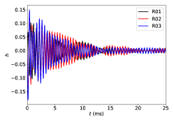
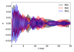
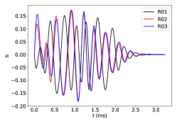
Figure 3: Post merger signal $h$ from simulations from the CoRe database performed at three different resolutions. From left to right, the panels respectively correspond to simulations with mass-ratios $q=1.0$, $0.5$, and $1.0$; total masses of $2.75M_{\odot}$, $2.88M_{\odot}$, and $2.70M_{\odot}$; and use the MS1b (left and middle) and SLy (right panel) EOSs. (They are respectively labelled BAM0070, BAM0094, and BAM0100 in the CoRe database, see Ref. Dietrich et al. (2018) for more details.) The black, red, and blue curves in each panel correspond to simulations with the same physical parameters, but with increasing numerical resolution. From left to right, computing the match between low and high resolution (medium and high resolution) for each case, we obtain, respectively, 0.11, 0.52, and 0.20 (0.12, 0.56, and 0.95).

To summarize, our training data consist of 123 $(M,h)$ pairs, where $h$ is a 9-component vector describing a postmerger signal. This discards labels for the mass ratio, spins, EOS, and numerical resolutions, but keeps that of the total mass. This omitted information, however, gives rise to differences between the waveforms, so it (along with any other differences between simulations) should be understood as latent variables. In the following subsection, we construct a CVAE to model these waveforms and characterize the latent information.

III.2 Experiments

We model $p(h|M)$ with a CVAE with latent dimension $l=4$. The encoder and decoder are fully-connected networks with rectified linear unit nonlinearities. Exploring various hyperparameter choices, we find best performance with a 2-hidden-layer encoder with $(100,50)$ units, a decoder with inverted structure, and $\beta=0.003$.

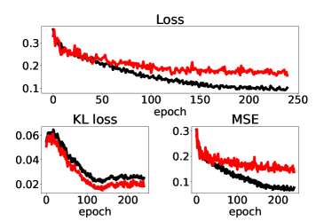
Figure 4: Training history for a CVAE trained with numerical waveforms in the representation (III.1). The upper plot shows the total loss (II), while the bottom two plots show the KL (left) and reconstruction loss (right) contributions to the total. The black and red curves correspond to the training and validation sets, respectively. The gap between training and validation sets is an indication of overfitting.

We split our dataset into training (60%) and validation (40%) sets, and train for 4000 epochs. The training history is plotted in Fig. 4. Since the validation loss is much higher than the training loss, we conclude that the CVAE is overfitting, and that the training set is too small for the network to successfully generalize to previously unseen waveforms. We have also tried methods for mitigating overfitting such as adding dropout layers. There was no significant improvements using that method.

IV Extended training set

Figure 5: The parameters in Eq. (III.1), obtained from fitting the numerical waveforms, versus compactness $\mathcal{C}$, color coded by the average mass $(\bar{M})$ of the two stars in units of solar mass. Since we do not have direct access to $\mathcal{C}$ from the simulations, here we define it be given by $f_{2}=(a_{9}+a_{10}\mathcal{C}+a_{11}\mathcal{C}^{2})(1.6\ M_{\odot}/\bar{M})$ with $a_{9}=-3.12$ kHz, $a_{10}=51.90$ kHz, and $a_{11}=-89.07$ kHz. We then fit for the parameters of $f_{1}=(a_{5}+a_{6}\mathcal{C}+a_{7}\mathcal{C}^{2}+a_{8}\mathcal{C}^{3})(1.6\ M_{\odot}/\bar{M})$ with our data. The blue curve in the $f_{1}$ plot represents the fit from Ref. Bose et al. (2018). Though this curve roughly lies within the range of the data points, we find different values for the best fit parameters for the mean of $f_{1}$. The remaining parameters, on the other hand, appear to be roughly linear in $\mathcal{C}$, with some noise. We overlay the fiducial model at a fixed $\bar{M}=1.35\ M_{\odot}$ on the numerical data: the solid red line is the mean of the data, i.e. $\vec{A}\cdot\mathcal{C}+\vec{B}$, while the shaded regions are the one standard deviation ranges. From this, we see that the fiducial model captures most of the numerical data.

The number of available numerical simulations is at present too small to properly train a CVAE to model postmerger waveforms. Nevertheless, we can assess the viability of the approach for the future by training on synthetic data. In this section, we first construct a “fiducial” waveform model $p_{\text{fid}}(h|\bar{M},\mathcal{C})$ based on the CoRe waveforms. The fiducial model depends on the average mass $\bar{M}=(M_{1}+M_{2})/2$ and the compactness $\mathcal{C}=GM/(Rc^{2})$ of the remnant neutron star. We then generate a much larger training set by sampling from this model, and we show that with this we can train the CVAE to have similar statistical properties as the fiducial model. This exercise also provides an estimate for the number of numerical waveforms needed to train a CVAE.

IV.1 Fiducial model

We now construct the fiducial model $p_{\text{fid}}(h|\bar{M},\mathcal{C})$ for postmerger waveforms $h$ given $\bar{M}$ and $\mathcal{C}$. We do not have direct access to $\mathcal{C}$ from the numerical-relativity simulations, so instead we extract it based on the dominant postmerger frequency Lehner et al. (2016a); Bose et al. (2018); Rezzolla and Takami (2016). Indeed, Ref. Bose et al. (2018) found that, for a remnant with $\bar{M}=1.6\leavevmode\nobreak\ \mathrm{M}_{\odot}$, the dominant postmerger frequencies approximately satisfy the relations,

$$f_{1} =\left(a_{5}+a_{6}\mathcal{C}+a_{7}\mathcal{C}^{2}+a_{8}\mathcal{C}^{3}\right)(1.6\ M_{\odot}/\bar{M}),$$ (12)

$$f_{2} =\left(a_{9}+a_{10}\mathcal{C}+a_{11}\mathcal{C}^{2}\right)(1.6\ M_{\odot}/\bar{M}),$$ (13)

with the numerical parameters $a_{5}=-35.17$ kHz, $a_{6}=727.99$ kHz, $a_{7}=-4858.54$ kHz, $a_{8}=10989.88$ kHz, $a_{9}=-3.12$ kHz, $a_{10}=51.90$ kHz, and $a_{11}=-89.07$ kHz. On dimensionful grounds, we have added an extra factor $1/\bar{M}$ to extend these relations to other BNS masses. We therefore take Eq. (13) as given and use it to define $\mathcal{C}$ in terms of $f_{2}$ and $\bar{M}$. After solving for $\mathcal{C}$, we plot all the parameters from fitting Eq. (III.1) to the numerical waveforms versus $\mathcal{C}$ in Fig. 5. The parameters of $f_{1}$ are then fitted to our data. We find $a_{5}=11.26$ kHz, $a_{6}=-284.83$ kHz, $a_{7}=2515.07$ kHz, and $a_{8}=-6800.26$ kHz. These values are different from the ones found in Ref. Bose et al. (2018), but as can be seen in Fig. 5, the curve defined by Bose et al. (2018) is within one standard deviation of the parameters we find.

We fit a generalized linear model for the remaining waveform parameters in terms of the compactness, i.e.,

$$\begin{pmatrix}\alpha_{1}\\ \alpha_{2}\\ \log(\tau_{1})\\ \log(\tau_{2})\\ \frac{\bar{M}}{1.6M_{\odot}}f_{1}\\ \frac{\bar{M}}{1.6M_{\odot}}f_{2}\\ \beta_{2}\\ \frac{\bar{M}^{2}}{1.6M_{\odot}}\gamma_{2}\\ \frac{\bar{M}^{3}}{1.6M_{\odot}}\xi_{2}\\ \end{pmatrix}\sim\mathcal{N}(\vec{B}+\vec{A}\mathcal{C},\Sigma),$$ (14)

where

$$\vec{A} =\begin{pmatrix}a_{1}\\ a_{2}\\ a_{3}\\ a_{4}\\ \left(a_{5}/\mathcal{C}+a_{6}+a_{7}\mathcal{C}+a_{8}\mathcal{C}^{2}\right)\\ \left(a_{9}/\mathcal{C}+a_{10}+a_{11}\mathcal{C}\right)\\ a_{12}\\ a_{13}\\ a_{14}\end{pmatrix},$$ (15)

$$\vec{B} =\begin{pmatrix}b_{1}\\ b_{2}\\ b_{3}\\ b_{4}\\ b_{5}\\ b_{6}\\ b_{7}\\ b_{8}\\ b_{9}\end{pmatrix},$$ (16)

and where $\Sigma$ is a generic covariance matrix, and $a_{i}$ and $b_{i}$ are constants which are obtained by fitting the numerical waveforms except for $\{a_{5},a_{6},a_{7},a_{8},a_{9},a_{10},a_{11}\}$, where we use the values discussed previously. We determine $\Sigma$ by first subtracting the mean of $\{\alpha_{1},\alpha_{2},\log(\tau_{1}),\log(\tau_{2}),\beta_{2},\gamma_{2},\xi_{2}\}$, and subtracting Eq. (12) and Eq. (13) for the frequencies. This method of computing $\Sigma$ is conservative in the sense that it overestimates the noise in the model. The covariance matrix can also be estimated by first removing $\vec{A}\cdot\mathcal{C}+\vec{B}$ from the data, or by simultaneously fitting for the linear dependence and covariance. However, we have checked that doing the former only reduces the magnitude of the covariance $\sim 2\%$, and does not significantly affect the results of the estimate.

Note that we took logarithms of $\tau_{1}$ and $\tau_{2}$ so as to normalize their distributions. The values of the parameters are recorded in appendix E. We add a factor of $1/\bar{M}$ in the frequencies to roughly model mass dependence of the frequency on the mass, inspired by Ref. Lehner et al. (2016a). The estimated variance in $\gamma_{2}$ and $\xi_{2}$ is large, which can lead to issues with the waveforms at late times. On dimensional grounds, we also add a factor of $1/\bar{M}^{2}$ to $\gamma_{2}$ and $1/\bar{M}^{3}$ to $\xi_{2}$.

We underline the fact that due to the stochastic nature of this model, even fixing $\bar{M}$ and $\mathcal{C}$, we will obtain different waveforms with each realization. Generating a large set of realizations of the fiducial model with these quantities fixed, we find that average match between the waveforms is $0.38$. These is similar to the values obtained when varying numerical resolutions in the simulations shown in Fig. 3, and thus representative of the large theoretical uncertainties. Furthermore, when training a CVAE on this fiducial model, we expect it to incorporate similar uncertainties: if the CVAE is well trained, then the CVAE model could recreate any of the waveforms from the fiducial model giving an average match close to $0.38$.

IV.2 Experiments

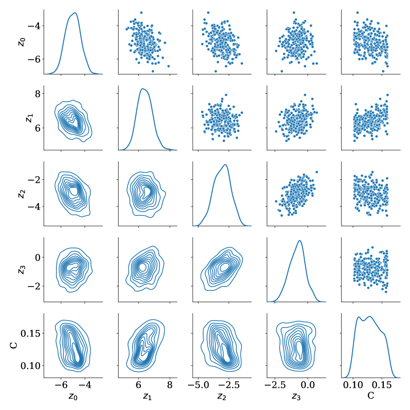
Figure 6: Pairplot of latent variables generated with data generated with the fiducial model with fixed masses and random compactness $\mathcal{C}\sim p(\mathcal{C})$. That is, we sample $h\sim p_{\text{fid}}(h|\bar{M}=1.35M_{\odot},\mathcal{C})$, then $z\sim p(z|\bar{M}=1.35M_{\odot},h)$. We can see that the CVAE is avoiding posterior collapse, which would be indicated by that data being independent of some latent variable. By looking at the compactness column one would hope to see a relationship between the compactness and the latent variables. Unfortunately the relationship is not obvious here.

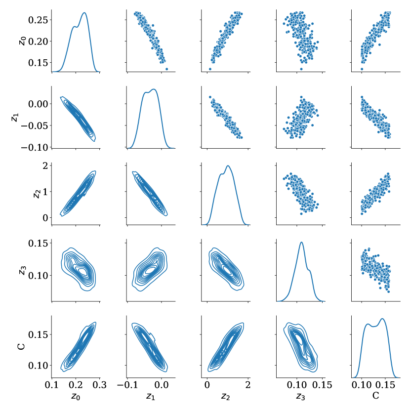
Figure 7: Similar to Fig. 6, but for the latent space of the CVAE trained on a fiducial model where the variance is reduced by half, i.e., $\Sigma\rightarrow 0.5\Sigma$. In this case, we can see that there is a roughly linear relationship between the latent variables and the compactness.

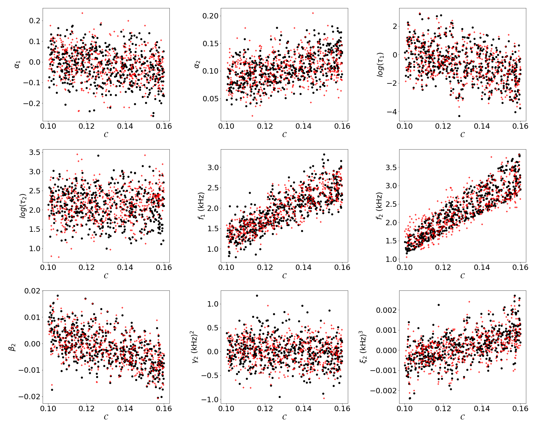
Figure 8: Parameters from the fiducial model with $1.2\ M_{\odot}<\bar{M}<1.7\ M_{\odot}$ and $\mathcal{C}\in(0.1,0.16)$ uniformly distributed (black dots), compared to the parameters recreated by the CVAE (red crosses). The recreated data is generated by inputting the fiducial model data into the CVAE. The CVAE was trained with 10,000 elements. Here we fix the value of $\beta=0.008$, which is different from the $\beta$ value used in Sec. III.2.

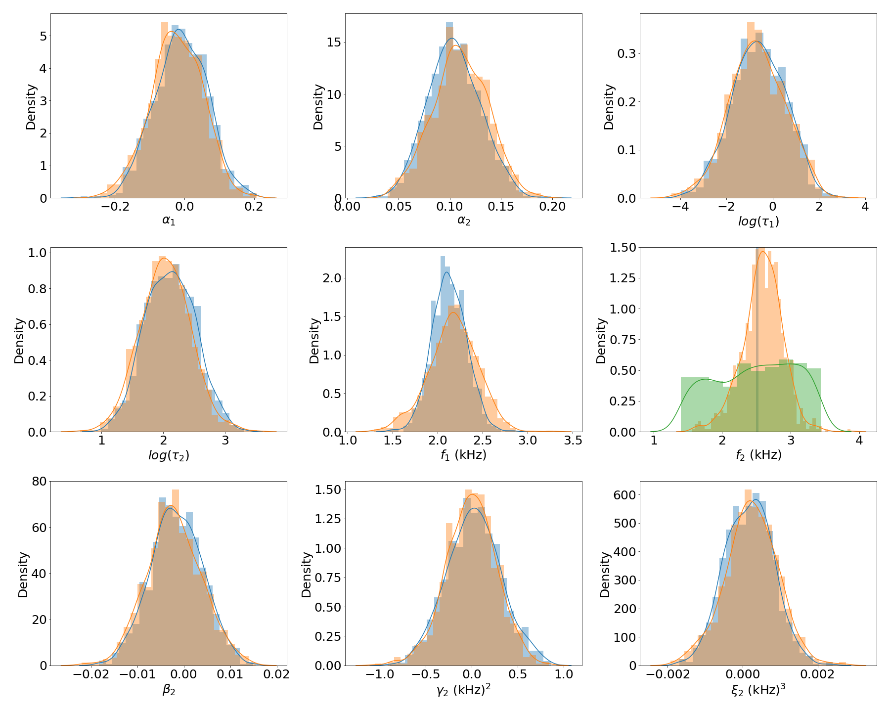
Figure 9: Probability density of fiducial model parameters (blue) and parameters recreated by the CVAE (orange) with fixed $\mathcal{C}=0.13$ and $\bar{M}=1.35\ M_{\odot}$. For the parameter $f_{2}$, there is no variance in the fiducial model when fixing $\mathcal{C}$ and $\bar{M}$, and for this figure we also show the fiducial model distribution with fixed $\bar{M}=1.35\ M_{\odot}$, but varying $\mathcal{C}$ (green). The recreated data is generated by inputting the fiducial model data into the CVAE. The CVAE was trained with 10,000 elements. Here we fix the value of $\beta=0.008$, which is different from the $\beta$ value used in Sec. III.2.

With the fiducial model, we are now able to generate artificial postmerger signals, which we take as training data for the CVAE. We first generate a dataset with 1,010,000 samples $h\sim p_{\text{fid}}(h|\bar{M},\mathcal{C})$ by randomly choosing the remnant mass, $1.2\ M_{\odot}<\bar{M}<1.7\ M_{\odot}$ and $\mathcal{C}\in(0.1,0.16)$ from uniform distributions. The dataset is then whitened and normalized. We then train CVAEs (with $l=4$) using 500, 1000, 5000, 8000, 9000, $10^{4}$, $1.5\times 10^{4}$, $10^{5}$, and $10^{6}$ elements. We set aside $10^{4}$ elements for the validation set. We train the CVAE with a batch size of 150 and use early stopping to terminate the training when the loss function becomes stagnant Goodfellow et al. (2016). Details of the CVAE architecture are provided in Appendix E.

We find that training the CVAE with a dataset with more than $10,000$ elements shows close to no signs of overfitting. The match from the input and recreated waveforms is low, with $\mathcal{M}\sim 0.27$ for the training set, and $\mathcal{M}\sim 0.24$ for the validation set. Despite the low matches, we find that the CVAE is still able to recreate the distribution of the parameters, see Fig. 8, indicating that the CVAE is functional. As noted above, given the stochastic nature of the fiducial model, which itself has $\mathcal{M}\sim 0.38$, the match is not the best metric to evaluate the performance of the CVAE.

What is more important then the average match is that the distribution of parameters reproduced by the CVAE is similar to the ones from the fiducial model. By looking at Fig. 8, we see that the recreated parameters from the CVAE (red crosses) are indeed similar to the input parameters (black dots). Furthermore, Fig. 9 shows that the CVAE learns the distributions of the parameters when fixing the fiducial model arguments $(\mathcal{C}=0.13,\bar{M}=1.35\ M_{\odot})$.

The only parameter where the distribution the CVAE recreates differs significantly from that of the fiducial model is $f_{2}$, which has no variance in the fiducial model when fixing $\mathcal{C}$ and $\bar{M}$. Though nonzero, the CVAE variance in $f_{2}$ at fixed $\mathcal{C}$ and $\bar{M}$ is still smaller than the variance of the fiducial model when only fixing $\bar{M}$ (green curve in the $f_{2}$ panel of Fig. 9). We also note that when allowing $\bar{M}$ to vary over the range 1.2 to 1.7 $M_{\odot}$, but still keeping $\mathcal{C}=0.13$, the standard deviation in $f_{2}$ for the CVAE is $\sim 15\%$ larger than when $\bar{M}$ is fixed to $1.35\ M_{\odot}$. This is roughly the increase expected from adding in quadrature the fiducial model variance in $f_{2}$ when varying $\bar{M}$.

For a given realization of the fiducial model, it is still possible to get a good match using the CVAE by searching over the latent space. We found that, for most cases, a waveform from the CVAE with $\mathcal{M}>0.90$ could be found by sampling the latent space randomly. And it would straightforward to implement a more sophisticated search algorithm for the correct latent variables which could increase this value. This indicates that the CVAE is sufficiently flexible so as to be able to recreate different realizations of the fiducial model despite the large variance in these realizations representing large theoretical uncertainties in the the training data.

We can now address the question of how the CVAE encodes information about the remnant compactness in the latent space. In Fig. 6, we plot the latent distribution of encoded waveforms $h\sim p(\bar{M},\mathcal{C})$ for fixed $\bar{M}=1.35$ $M_{\odot}$, but sampling $\mathcal{C}\sim p(\mathcal{C})$. We see that the latent variables clearly encode information, as they trace a path in the latent space rather than sampling the normal distribution. However, there is no obvious connection to the compactness $\mathcal{C}$.

To probe whether correlations between $z$ and $\mathcal{C}$ can be obtained under more idealized conditions, we train the CVAE once again, but this time based on a fiducial model with a reduced noise level. Figure 7 shows the latent space of the CVAE trained with the noise variance reduced by half, i.e., $\Sigma\rightarrow 0.5\Sigma$. We see that there is a clear correlation between the latent variables and $\mathcal{C}$. The CVAE has therefore learned about the compactness based on waveforms alone, without ever having been provided compactness information. This is evidence of the neural network learning the $\mathcal{C}-f_{2}$ relationship. While this is a simple relationship to uncover, it shows how the CVAE can expose interesting relationships in the latent space.

V Discussion

The detection of a gravitational wave signal from the post-merger oscillations of a BNS would be a major accomplishment with important consequences for our understanding of physics in extreme regimes. Given the weaker amplitude and high frequency of such a signal, a good model will be essential in making and learning from such a detection. However, our ability to build such a model is hampered by a number of theoretical uncertainties, including our lack of knowledge of the true neutron star EOS, uncertainties regarding the behavior of magnetized matter, viscosity, cooling, and other microphysical effects, and difficulties adequately resolving turbulence and other small scale effects, while still covering the allowed parameter space. Machine learning offers a way to build partially informed models with relatively few assumptions about the unknown physics. To build the CVAE, we assume that the unknown physics can be encoded in a small latent space, and that there is a way to interpolate between different theoretical models of the unknown physics. By training a neural network with samples covering not only different unknown physics (e.g. different EOSs), but also different theoretical errors (e.g. numerical resolutions used in the simulations), we can attempt to build a model that interpolates over both, and thus is sufficiently robust to be used to look for real signals. The neural network approach also easily adapts to incorporate new information as it is obtained, and does so with a low associated computational cost at training time. In this approach, the main cost lies in the amount of data that is required to train the model. In this case, training the model with $10^{6}$ elements took approximately three days on a laptop. This training time can be reduced significantly by taking advantage of GPUs.

By building CVAEs for toy model data, we showed that the CVAE is capable of learning simple waveform time series consisting of a sum of sine functions (see Appendix B). We then moved on to training the CVAE on real numerical waveforms using the CoRe database Dietrich et al. (2018), and found that the neural network is overfitting, which is unsurprising given the dearth of data to train on, and the complexity of the waveforms. Instead of training directly on the time series from the numerical waveforms, we fit a nine parameter function [Eq. (III.1)] to waveforms, and used these parameters as the training data. We combined this with some preprocessing to improve the learning outcome, but still found that we were overfitting. Given that we could not avoid overfitting with the data we had, we turned our attention to estimating how much data would be required for the CVAE to work. To perform the estimate, we built a stochastic fiducial model of the parameters to generate data to train on. We generated data using the fiducial model, trained a CVAE with four latent variables, and found that we could recreate the distribution of the parameters with $\sim 10,000$ waveforms. The particular choice of fitting function we used was chosen mainly for illustration, and other choices, for example, using a greater number of free parameters, should also work with these methods, though would presumably increase the required size of the training set.

In investigating the latent space generated by the training process, we found evidence that the latent space was encoding the hidden variables, but we were unable to obtain a clear correspondence between the main hidden variable (the neutron star compactness) and some combination of the latent variables. A readily apparent relationship does show up once the noise of the fiducial model is reduced. This suggests that in the case without reduced noise, the latent space still encodes the compactness, but in a more complicated way. This relation could perhaps be found by training a secondary neural network for this purpose. We leave further study of the latent space to future work.

In this work, we considered two ways to present the data to the neural network: the full time series, and the parameters of a model which was fit to the time series. However, these are far from the only choices. Another method which we attempted, but found poor results for, is to decompose the spectrum of the waveforms with principle component analysis Clark et al. (2016), and then train on the coefficients. We found that we needed more than 10 principle components to get a match above 0.90. The combination of large variance and needing many coefficients made the learning of the data more difficult.

It is also important to keep in mind that the estimate given in Sec. IV.2 depends heavily on the specific neural network architecture (number of layers, number of neurons per layer, etc.) that we train on. The space of neural network implementations of a CVAE is large, and the one we picked might not be the optimal one despite our search. One could envision trying to adapt tools such as autoML Jin et al. (2018), which searches over the space of neural networks, to build a CVAE optimal for the post-merger data.

From our studies, we conclude that more training data is required to train the CVAE to properly represent BNS post-merger waveforms. We estimate that $\sim 10^{4}$ waveforms are needed. Though one direction for future work would be to incorporate additional simulation waveforms catalogs (e.g. Kiuchi et al. (2020)), this is still close to two orders of magnitude more than are presently available. Further optimizations to the CVAE architecture could potentially reduce this requirement, as could improved accuracy in the simulations which would reduce the variance in the waveforms. We note that here we have attempted to incorporate truncation errors effects in a simple way by including simulations with the same parameters at multiple resolution as equal data. This could be done in a more sophisticated way by weighting higher resolutions more, or otherwise incorporating truncation error estimates, though this can be challenging in cases that lack formal convergence in the discretization scale of the simulation. Given the computational cost associated with each simulation, accumulating enough waveforms to train a neural network could be achievable, but would require a large-scale, coordinated effort from the simulation community. A properly trained CVAE could play an important role in mapping out the relationships between different variables in the space of BNS post-merger waveforms.

Appendix A Waveform model with partial information

Thanks to numerous developments in solving the equations of general relativity, the binary black hole waveform is largely known (for comparable mass ratios). The corresponding waveform models, whether they are constructed phenomenologically by matching numerical waveforms with analytical approximations, or through other methods such as the effective-one-body approach, are all determined uniquely for every set of binary parameters. On the other hand, to construct the waveform model for post-merger neutron stars, we are facing a different problem where our current knowledge is insufficient to predict an accurate waveform given the orbital parameters. This problem is likely to persist until there are significant improvements in our understanding of the neutron star EOS (which likely will come from the detections themselves) and in our modelling of the merger/post-merger process with a sufficiently complete physical prescription.

Nevertheless, although current numerical simulations do not provide the full answer, they do converge on certain features (such as the dominant peak in the post-merger spectrum). It is natural to ask how one could construct a waveform model utilizing this partial information, while taking into account the inherent uncertainties. To answer this question, we present a general framework for waveforms with partial information.

A waveform model with theoretical uncertainties can be written as $h=h({C};\mathcal{I})$. The control variables ${C}$ are the physical quantities that determine the waveform assuming perfect knowledge. In the binary case, they are the orbital parameters, which can be determined from the inspiral waveform measurement (which in general will be much louder than the post-merger signal) to a certain accuracy. The latent variables $\mathcal{I}$ encapsulate all the theoretical uncertainties and modelling errors. In the limit that a waveform model becomes completely determined without theoretical uncertainties, ${\rm dim}(\mathcal{I})=0$.

A.1 Detection

For the purpose of detection, the control variables are already constrained by the inspiral measurement. As a result, the posterior distribution of the control variables $P_{\rm in}({C})$ can be used as a prior distribution for post-merger detection. One way to quantify the statistical significance of a post-merger event detection is using the hypothesis test framework. Using the post-merger gravitational wave data stream $s$, we compare the following two hypotheses:

$$\mathcal{H}_{1}:s=h+n\,,$$

$$\mathcal{H}_{2}:s=n\,$$ (17)

where $n$ represents noise.

The significance of detection can be characterized by the Bayes factor, which is defined as

$$\mathcal{B}:=\frac{P(s|\mathcal{H}_{1})}{P(s|\mathcal{H}_{2})}\,,$$ (18)

and the evidence function $P(s|\mathcal{H}_{i})$ can be computed by

$$P(s|\mathcal{H}_{i})=\int d{C}d\mathcal{I}\mathcal{L}_{i}({C},\mathcal{I})P_{\rm in}({C})P_{\rm in}(\mathcal{I})\,,$$ (19)

where $P_{\rm in}(\mathcal{I})$ is the prior weight function for the latent variables. The likelihood function $\mathcal{L}_{i}$ is given by

$$\mathcal{L}_{1}=\frac{1}{Z_{n}}\prod_{f>0}{\rm exp}\left(-\frac{2|s-h|^{2}}{S_{n}}\right)\,,$$

$$\mathcal{L}_{2}=\frac{1}{Z_{n}}\prod_{f>0}{\rm exp}\left(-\frac{2|s|^{2}}{S_{n}}\right)\,,$$ (20)

where $S_{n}$ is the single-side spectral density of the detector, and $Z_{n}$ is a common normalization constant. The larger the Bayes factor is, the more significant the detection. According to the Jeffreys scale of interpretation of Bayes Factor Jeffreys (1961), the evidence is “very strong” if $\mathcal{B}>10$.

Even without prior knowledge of the control variables, we can still define the SNR of an event as

$${\rm SNR}:=2{\rm Max}_{{C},\mathcal{I}}\left(\int df\frac{h({C},\mathcal{I})s^{*}+h.c.}{S_{n}}\right)\,.$$ (21)

Given a threshold in SNR, it is straightforward to evaluate the average rate of detecting a false signal due to the detector noise background, which is often referred to as the false-alarm rate. This part is similar to binary black hole detection. Generally speaking, for a given false alarm rate, the threshold SNR is higher if the latent space is larger.

A.2 Parameter estimation

While we will not focus on using the model discussed in this paper for parameter estimation, here we briefly outline how such a waveform model with partial information might be used for parameter estimation. After we compute the posterior distribution of ${C}$ and $\mathcal{I}$ based on the gravitational-wave data $s$, the posterior distribution of the control variables can be obtained by marginalizing the latent variables:

$$P({C}|s)=\int d\mathcal{I}P({C},\mathcal{I}|s)\,.$$ (22)

In reality, the computational cost for constructing the posterior distribution of ${C}$ and $\mathcal{I}$ increases with the size of the latent space. Therefore, an efficient waveform model with theoretical uncertainties should minimize the size of the latent space while still being able to fit the true waveforms.

The latent space encodes information about the unknown physical parameters and so it is also possible to use the latent space to infer the unknown physical parameters. This can be accomplished if a map between the unknown physical parameters and latent space is built. In general this is not an easy task as the mapping can be quite complicated, but we have seen that this is possible in Fig. 7 with our fiducial model.

Appendix B Toy Model

As a simple demonstration of a CVAE being used as a generative model, we train a CVAE on toy data which consists of a sum of sine functions. This is motivated by the observation that the post-merger waveform seems to be dominated by a small number of main frequencies which are believed to not vary significantly in time Clark et al. (2016).

We generate $\mathcal{O}(10^{3})$ waveforms of the form

$$w=\sum_{i=1}^{3}\sin(\omega_{i}t+\phi_{i})$$ (23)

where $\phi_{i}\in[0,2\pi]$ and $\omega_{i}\in[1,4]$, $t\in[0,15]$ with a sample frequency of $1000/15$. The phase and frequencies are picked randomly from a uniform distribution. The data set is then split into a training and a testing set. We randomly pick $60\%$ of the total set for training, and the other $40\%$ as the testing set. Once the network is trained, we measure the match using Eq. 11.

We train the neural network using the frequencies as the conditional variables and let the latent space have three variables. The neural network has three encoding layers with $\{100,50,10\}$ neurons in the layers. The decoder has the same structure but inverted. The encoder and decoder have rectified linear unit functions as the activation functions, and the latent and output have linear functions as activation functions. Figure 10 is an example output of the waveform recreated by the CVAE. We found that the CVAE was easily able to recreate the waveform given sufficient amounts of data ($\sim 600$ waveforms).

Figure 10: A comparison of the waveform generated by Eq. (23) (black curve) to the one recreated by the CVAE (red curve). The waveform is produced by sampling the latent space and picking the latent variables which produce the highest match. The match is 0.95.

Figure 11: To see that the latent space learned information about the parameters $\phi_{i}$ we generate a new wave using Eq. (23) with the same $\omega_{i}$ as Fig 10 but different $\phi_{i}$. We search over our latent space to see if we can also recreate that waveform. Here we see the waveform generated by Eq. (23) (black curve) could be recreated by the CVAE (red curve).

Appendix C Fitting in time domain

In this section, we discuss the issues of training the CVAE directly on the numerical waveforms. We show that training directly on the numerical waveforms with the amount of data we have leads to overfitting.

We constructed a CVAE similar to the one in Sec. 23, where the input layer took in the time series of the numerical waveform. The training set consisted of the numerical waveforms and we augmented the dataset by adding random phases to the waveforms. Using this method we increased our dataset to 500 elements.

After training, we compute the match of the recreated waveforms, finding that the neural network was in fact capable of recreating the waveforms it trained on, but could not interpolate between different waveforms. That is, the neural network was overfitting. The overfitting can be seen in Fig. 12 where we have the history of the mean square error throughout the training. We see that the mean square error of the training and testing sets is diverging, indicating that the CVAE is learning the training set well, but is not able to interpolate. This is expected given the small amount of training data. In the following section, we will discuss methods to alleviate this problem, and provide an estimate of the amount of data required for this model to function.

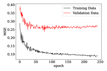
Figure 12: Training history of the CVAE with time domain numerical waveform data. The plot depicts the mean square error contribution of the loss function, that is how well can it recreate the waveform. The difference between the training data and validation data is a symptom of overfitting.

Appendix D Data preprocessing

In this section, we discuss the details of the data processing done to the data in the main text. The technique used here to preprocess the data is called data whitening; the basic idea is to center the dataset, normalize it, and remove the correlations.

Certain subsets of the parameters in the model given by Eq. (III.1) turn out to be strongly correlated. This is illustrated by the correlation matrix (Fig. 13) of the data. Intuitively, you would suspect that this would make it easier for the CVAE to reproduce the data. This turns out to not be completely true since it creates an incentive to only learn the highly correlated parameters and disregard the uncorrelated ones. This occurs since the correlated terms end up dominating the mean square term of the cost function. We also found that our data tends toward posterior collapse when the correlations are left as is.

To deal with these issues, we can use some basic data processing methods such as the whitening transform. This transformation consists of three steps: (i) centering the dataset, (ii) decorrelating the dataset, and (iii) rescaling the dataset. To center the dataset, we simply find the mean of every feature and subtract it from the dataset. This guarantees that the mean of the new dataset is 0. To decorrelate the data we find the eigenvalues $\lambda_{i}$ and eigenvectors $v_{i}$ of the covariance matrix and define $V=[v_{1},v_{2},...,v_{n}]$ where the columns are the eigenvectors. The decorrelated data $X_{\rm dec}$ is found with respect to the original data $X$ by projecting $X$ on $V$:

$$X_{\rm dec}=X\cdot V\ .$$ (24)

Finally, to rescale the data, we divide through by the eigenvalues by defining the diagonal matrix $P={\rm diag}(1/\sqrt[]{\lambda_{1}+\epsilon},1/\sqrt[]{\lambda_{2}+\epsilon},...,1/\sqrt[]{\lambda_{n}+\epsilon})$,

$$X_{\rm whiten}=X_{\rm dec}\cdot P$$ (25)

where $X_{\rm whiten}$ is the whitened data, and $\epsilon$ is a small number to deal with the cases where the eigenvalue is zero (though this does not arise for the cases we consider). Once the data is whitened, we can also tune the parameter $\beta$ in the cost function such that no posterior collapse occurs. The tuning of the parameter is done by varying the parameter over many training sessions to find the optimal value Higgins et al. (2017). After performing these steps, the correlation matrix of the transformed data will just be the identity matrix.

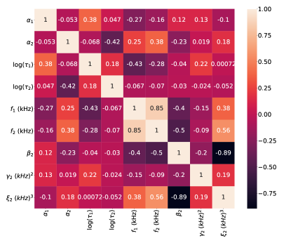
Figure 13: Normalized covariance matrix of the parameters defined in Eq. (III.1), when fitted to the numerical relativity waveforms.

Appendix E Fiducial Model and CVAE Parameters

Tables 1 and 2 give the parameters for Eq. (14) presented in Sec. IV.1 by fitting the numerical waveforms from the CoRe database Dietrich et al. (2018). The fits are found by first finding the compactness using the $f_{2}$ - $\mathcal{C}$ relation. Then we fit $f_{1}$ with the compactness to Eq. (12), and perform a linear fit to the other parameters. This gives us the vectors $\vec{A}$ and $\vec{B}$, with the specific values shown in Tables 1 and 2. We then compute the covariance matrix $\Sigma$, finding the values shown in Table 3.

$a_{1}$	$a_{2}$	$a_{3}$	$a_{4}$	$a_{5}$	$a_{6}$	$a_{7}$	$a_{8}$	$a_{9}$	$a_{10}$	$a_{11}$	$a_{12}$	$a_{13}$	$a_{14}$
-0.99	0.78	2.73	2.41	11.26	-284.83	2515.07	-6800.25	-3.12	51.90	89.07	-0.03	-2.22	0.04

Table 1: Parameters for $\vec{A}$ in the fiducial model

$b_{1}$	$b_{2}$	$b_{3}$	$b_{4}$	$b_{5}$	$b_{6}$	$b_{7}$	$b_{8}$	$b_{9}$
0.12	$3\times 10^{-4}$	2.73	2.42	0.00	0.00	0.04	0.31	$-5\times 10^{-3}$

Table 2: Parameters for $\vec{B}$ in the fiducial model

$8.23\times 10^{-3}$	$-1.54\times 10^{-4}$	$4.95\times 10^{-2}$	$2.19\times 10^{-3}$	$-4.39\times 10^{-3}$	$4.28\times 10^{-3}$	$1.08\times 10^{-4}$	$4.85\times 10^{-3}$	$-1.20\times 10^{-5}$
$-1.54\times 10^{-4}$	$1.00\times 10^{-3}$	$-3.04\times 10^{-3}$	$-6.87\times 10^{-3}$	$-8.23\times 10^{-4}$	$-3.41\times 10^{-3}$	$-7.05\times 10^{-5}$	$2.55\times 10^{-4}$	$7.06\times 10^{-6}$
$4.95\times 10^{-2}$	$-3.04\times 10^{-3}$	$2.01$	$1.28\times 10^{-1}$	$-8.74\times 10^{-2}$	$1.12\times 10^{-1}$	$-5.41\times 10^{-4}$	$1.29\times 10^{-1}$	$1.30\times 10^{-6}$
$2.19\times 10^{-3}$	$-6.87\times 10^{-3}$	$1.28\times 10^{-1}$	$2.64\times 10^{-1}$	$-3.34\times 10^{-3}$	$8.79\times 10^{-3}$	$-1.48\times 10^{-4}$	$-5.18\times 10^{-3}$	$-3.41\times 10^{-5}$
$-4.39\times 10^{-3}$	$-8.23\times 10^{-4}$	$-8.74\times 10^{-2}$	$-3.34\times 10^{-3}$	$2.92\times 10^{-2}$	$-2.66\times 10^{-15}$	$5.44\times 10^{-5}$	$-1.05\times 10^{-2}$	$-3.34\times 10^{-5}$
$4.28\times 10^{-3}$	$-3.41\times 10^{-3}$	$1.12\times 10^{-1}$	$8.79\times 10^{-3}$	$-2.66\times 10^{-15}$	$7.24\times 10^{-2}$	$1.32\times 10^{-3}$	$9.34\times 10^{-3}$	$-1.96\times 10^{-4}$
$1.08\times 10^{-4}$	$-7.05\times 10^{-5}$	$-5.41\times 10^{-4}$	$-1.48\times 10^{-4}$	$5.44\times 10^{-5}$	$1.32\times 10^{-3}$	$9.19\times 10^{-5}$	$-7.99\times 10^{-4}$	$-1.09\times 10^{-5}$
$4.85\times 10^{-3}$	$2.55\times 10^{-4}$	$1.29\times 10^{-1}$	$-5.18\times 10^{-3}$	$-1.05\times 10^{-2}$	$9.34\times 10^{-3}$	$-7.99\times 10^{-4}$	$1.75\times 10^{-1}$	$1.01\times 10^{-4}$
$-1.20\times 10^{-5}$	$7.06\times 10^{-6}$	$1.30\times 10^{-6}$	$-3.41\times 10^{-5}$	$-3.34\times 10^{-5}$	$-1.96\times 10^{-4}$	$-1.09\times 10^{-5}$	$1.01\times 10^{-4}$	$1.61\times 10^{-6}$

Table 3: Elements of the covariance matrix $\Sigma$ in the fiducial model

Finally, the details of the CVAE used in Sec. IV.2 are given in Table 4.

	Input	Layer 1	Layer 2	Latent Layer	Layer 3	Layer 4	Output
Number of Neurons	9	345	335	4	335	345	9
Activation Function	–	ReLu	ReLu	Linear	ReLu	ReLu	tanh
Type		Dense	Dense	Lambda	Dense	Dense

Table 4: Parameters for the CVAE used in Sec. IV.2. All the layers in the neural network consist of dense layers, except for the latent space where we have a lambda layer which takes the output of layer 2 as the mean and variance of a multivariate normal and outputs a sample from the multivariate normal.

References

- Abbott et al. (2019) B. P. Abbott et al. (LIGO Scientific, Virgo), Phys. Rev. X 9, 031040 (2019), arXiv:1811.12907 [astro-ph.HE] .
- Abbott et al. (2021a) R. Abbott et al. (LIGO Scientific, Virgo), Phys. Rev. X 11, 021053 (2021a), arXiv:2010.14527 [gr-qc] .
- Abbott et al. (2021b) R. Abbott et al. (LIGO Scientific, VIRGO, KAGRA), (2021b), arXiv:2111.03606 [gr-qc] .
- Abbott et al. (2017a) B. P. Abbott et al. (LIGO Scientific, Virgo), Phys. Rev. Lett. 119, 161101 (2017a), arXiv:1710.05832 [gr-qc] .
- Abbott et al. (2020a) B. P. Abbott et al. (LIGO Scientific, Virgo), Astrophys. J. Lett. 892, L3 (2020a), arXiv:2001.01761 [astro-ph.HE] .
- Abbott et al. (2020b) R. Abbott et al. (LIGO Scientific, Virgo), Astrophys. J. Lett. 896, L44 (2020b), arXiv:2006.12611 [astro-ph.HE] .
- Abbott et al. (2021c) R. Abbott et al. (LIGO Scientific, KAGRA, VIRGO), Astrophys. J. Lett. 915, L5 (2021c), arXiv:2106.15163 [astro-ph.HE] .
- Meidam et al. (2014) J. Meidam, M. Agathos, C. Van Den Broeck, J. Veitch, and B. S. Sathyaprakash, Phys. Rev. D90, 064009 (2014), arXiv:1406.3201 [gr-qc] .
- Yang et al. (2018) H. Yang, V. Paschalidis, K. Yagi, L. Lehner, F. Pretorius, and N. Yunes, Phys. Rev. D97, 024049 (2018), arXiv:1707.00207 [gr-qc] .
- Yang et al. (2017) H. Yang, K. Yagi, J. Blackman, L. Lehner, V. Paschalidis, F. Pretorius, and N. Yunes, Phys. Rev. Lett. 118, 161101 (2017), arXiv:1701.05808 [gr-qc] .
- Brito et al. (2018) R. Brito, A. Buonanno, and V. Raymond, Phys. Rev. D98, 084038 (2018), arXiv:1805.00293 [gr-qc] .
- Messenger and Read (2012) C. Messenger and J. Read, Phys. Rev. Lett. 108, 091101 (2012), arXiv:1107.5725 [gr-qc] .
- Bustillo et al. (2020) J. C. Bustillo, T. Dietrich, and P. D. Lasky, “Higher-order gravitational-wave modes will allow for percent-level measurements of hubble’s constant with single binary neutron star merger observations,” (2020), arXiv:2006.11525 [gr-qc] .
- Miao et al. (2018) H. Miao, H. Yang, and D. Martynov, Phys. Rev. D 98, 044044 (2018), arXiv:1712.07345 [gr-qc] .
- Penrose (1969) R. Penrose, Nuovo Cimento Rivista Serie 1 (1969).
- Sekiguchi et al. (2011) Y. Sekiguchi, K. Kiuchi, K. Kyutoku, and M. Shibata, Physical Review Letters 107 (2011), 10.1103/physrevlett.107.211101.
- Radice et al. (2017) D. Radice, S. Bernuzzi, W. D. Pozzo, L. F. Roberts, and C. D. Ott, The Astrophysical Journal 842, L10 (2017).
- Most et al. (2019) E. R. Most, L. J. Papenfort, V. Dexheimer, M. Hanauske, S. Schramm, H. Stöcker, and L. Rezzolla, Physical Review Letters 122 (2019), 10.1103/physrevlett.122.061101.
- Paschalidis (2017) V. Paschalidis, Classical and Quantum Gravity 34, 084002 (2017).
- Ruiz et al. (2016) M. Ruiz, R. N. Lang, V. Paschalidis, and S. L. Shapiro, The Astrophysical Journal 824, L6 (2016).
- Dall’Osso et al. (2014) S. Dall’Osso, B. Giacomazzo, R. Perna, and L. Stella, The Astrophysical Journal 798, 25 (2014).
- Shibata and Hotokezaka (2019) M. Shibata and K. Hotokezaka, Annual Review of Nuclear and Particle Science 69, 41–64 (2019).
- Hotokezaka et al. (2011) K. Hotokezaka, K. Kyutoku, H. Okawa, M. Shibata, and K. Kiuchi, Physical Review D 83 (2011), 10.1103/physrevd.83.124008.
- Bauswein et al. (2013) A. Bauswein, T. W. Baumgarte, and H.-T. Janka, Physical Review Letters 111 (2013), 10.1103/physrevlett.111.131101.
- Martynov et al. (2019) D. Martynov et al., Phys. Rev. D 99, 102004 (2019), arXiv:1901.03885 [astro-ph.IM] .
- Abbott et al. (2015) R. Abbott et al. (LIGO Scientific), Classical and Quantum Gravity 32, 074001 (2015).
- Acernese et al. (2015) F. Acernese et al. (VIRGO), Class. Quant. Grav. 32, 024001 (2015), arXiv:1408.3978 [gr-qc] .
- Abbott et al. (2017b) B. P. Abbott et al. (LIGO Scientific, Virgo), Astrophys. J. Lett. 851, L16 (2017b), arXiv:1710.09320 [astro-ph.HE] .
- Torres-Rivas et al. (2019) A. Torres-Rivas, K. Chatziioannou, A. Bauswein, and J. A. Clark, Phys. Rev. D99, 044014 (2019), arXiv:1811.08931 [gr-qc] .
- Flanagan and Hinderer (2008) E. E. Flanagan and T. Hinderer, Phys. Rev. D 77, 021502 (2008), arXiv:0709.1915 [astro-ph] .
- Bauswein et al. (2012) A. Bauswein, H. Janka, K. Hebeler, and A. Schwenk, Phys. Rev. D 86, 063001 (2012), arXiv:1204.1888 [astro-ph.SR] .
- Rezzolla and Takami (2016) L. Rezzolla and K. Takami, Physical Review D 93 (2016), 10.1103/physrevd.93.124051.
- Lehner et al. (2016a) L. Lehner, S. L. Liebling, C. Palenzuela, O. L. Caballero, E. O’Connor, M. Anderson, and D. Neilsen, Class. Quant. Grav. 33, 184002 (2016a), arXiv:1603.00501 [gr-qc] .
- Kingma and Welling (2013) D. P. Kingma and M. Welling, “Auto-encoding variational bayes,” (2013), arXiv:1312.6114 [stat.ML] .
- Clark et al. (2016) J. A. Clark, A. Bauswein, N. Stergioulas, and D. Shoemaker, Class. Quant. Grav. 33, 085003 (2016), arXiv:1509.08522 [astro-ph.HE] .
- Bose et al. (2018) S. Bose, K. Chakravarti, L. Rezzolla, B. Sathyaprakash, and K. Takami, Physical Review Letters 120 (2018), 10.1103/physrevlett.120.031102.
- Cornish and Littenberg (2015) N. J. Cornish and T. B. Littenberg, Classical and Quantum Gravity 32, 135012 (2015).
- Breschi et al. (2019) M. Breschi, S. Bernuzzi, F. Zappa, M. Agathos, A. Perego, D. Radice, and A. Nagar, Phys. Rev. D 100, 104029 (2019), arXiv:1908.11418 [gr-qc] .
- Bauswein and Stergioulas (2015) A. Bauswein and N. Stergioulas, Phys. Rev. D91, 124056 (2015), arXiv:1502.03176 [astro-ph.SR] .
- Hanauske et al. (2017) M. Hanauske, K. Takami, L. Bovard, L. Rezzolla, J. A. Font, F. Galeazzi, and H. Stöcker, Phys. Rev. D96, 043004 (2017), arXiv:1611.07152 [gr-qc] .
- Lehner et al. (2016b) L. Lehner, S. L. Liebling, C. Palenzuela, and P. M. Motl, Phys. Rev. D94, 043003 (2016b), arXiv:1605.02369 [gr-qc] .
- Easter et al. (2018) P. J. Easter, P. D. Lasky, A. R. Casey, L. Rezzolla, and K. Takami, (2018), arXiv:1811.11183 [gr-qc] .
- Bauswein and Stergioulas (2019) A. Bauswein and N. Stergioulas, (2019), arXiv:1901.06969 [gr-qc] .
- Bernuzzi (2020) S. Bernuzzi, Gen. Rel. Grav. 52, 108 (2020), arXiv:2004.06419 [astro-ph.HE] .
- Soultanis et al. (2021) T. Soultanis, A. Bauswein, and N. Stergioulas, (2021), arXiv:2111.08353 [astro-ph.HE] .
- Tsang et al. (2019) K. W. Tsang, T. Dietrich, and C. Van Den Broeck, Phys. Rev. D 100, 044047 (2019), arXiv:1907.02424 [gr-qc] .
- Takami et al. (2015) K. Takami, L. Rezzolla, and L. Baiotti, Phys. Rev. D91, 064001 (2015), arXiv:1412.3240 [gr-qc] .
- Chua et al. (2019) A. J. K. Chua, C. R. Galley, and M. Vallisneri, Phys. Rev. Lett. 122, 211101 (2019), arXiv:1811.05491 [astro-ph.IM] .
- Khan and Green (2021) S. Khan and R. Green, Phys. Rev. D 103, 064015 (2021), arXiv:2008.12932 [gr-qc] .
- Chua et al. (2021) A. J. K. Chua, M. L. Katz, N. Warburton, and S. A. Hughes, Phys. Rev. Lett. 126, 051102 (2021), arXiv:2008.06071 [gr-qc] .
- Cuoco et al. (2021) E. Cuoco et al., Mach. Learn. Sci. Tech. 2, 011002 (2021), arXiv:2005.03745 [astro-ph.HE] .
- Gabbard et al. (2019) H. Gabbard, C. Messenger, I. S. Heng, F. Tonolini, and R. Murray-Smith, (2019), arXiv:1909.06296 [astro-ph.IM] .
- Goodfellow et al. (2016) I. Goodfellow, Y. Bengio, and A. Courville, Deep Learning (MIT Press, 2016) http://www.deeplearningbook.org.
- Kingma and Ba (2017) D. P. Kingma and J. Ba, “Adam: A method for stochastic optimization,” (2017), arXiv:1412.6980 [cs.LG] .
- Chen et al. (2017) X. Chen, D. P. Kingma, T. Salimans, Y. Duan, P. Dhariwal, J. Schulman, I. Sutskever, and P. Abbeel, “Variational lossy autoencoder,” (2017), arXiv:1611.02731 [cs.LG] .
- Higgins et al. (2016) I. Higgins, L. Matthey, A. Pal, C. Burgess, X. Glorot, M. Botvinick, S. Mohamed, and A. Lerchner, (2016).
- Bowman et al. (2016) S. R. Bowman, L. Vilnis, O. Vinyals, A. M. Dai, R. Jozefowicz, and S. Bengio, “Generating sentences from a continuous space,” (2016), arXiv:1511.06349 [cs.LG] .
- Kingma et al. (2017) D. P. Kingma, T. Salimans, R. Jozefowicz, X. Chen, I. Sutskever, and M. Welling, “Improving variational inference with inverse autoregressive flow,” (2017), arXiv:1606.04934 [cs.LG] .
- Dietrich et al. (2018) T. Dietrich, D. Radice, S. Bernuzzi, F. Zappa, A. Perego, B. Brueugmann, S. V. Chaurasia, R. Dudi, W. Tichy, and M. Ujevic, “Core database of binary neutron star merger waveforms and its application in waveform development,” (2018), arXiv:1806.01625 [gr-qc] .
- Jin et al. (2018) H. Jin, Q. Song, and X. Hu, “Auto-keras: An efficient neural architecture search system,” (2018), arXiv:1806.10282 [cs.LG] .
- Kiuchi et al. (2020) K. Kiuchi, K. Kawaguchi, K. Kyutoku, Y. Sekiguchi, and M. Shibata, Phys. Rev. D 101, 084006 (2020), arXiv:1907.03790 [astro-ph.HE] .
- Jeffreys (1961) H. Jeffreys, Theory of probability (Clarendon Press, Oxford, 1961).
- Higgins et al. (2017) I. Higgins, L. Matthey, A. Pal, C. Burgess, X. Glorot, M. Botvinick, S. Mohamed, and A. Lerchner, “beta-vae: Learning basic visual concepts with a constrained variational framework,” (2017).