Characterizing the breakdown of quasi-universality in the post-merger gravitational waves from binary neutron star mergers

Abstract

The post-merger gravitational wave (GW) emission from a binary neutron star merger is expected to provide exciting new constraints on the dense-matter equation of state (EoS). Such constraints rely, by and large, on the existence of quasi-universal relations, which relate the peak frequencies of the post-merger GW spectrum to properties of the neutron star structure in a model-independent way. In this work, we report on violations of existing quasi-universal relations between the peak spectral frequency, $f_{2}$, and the stellar radius, for EoSs models with backwards-bending slopes in their mass-radius relations (such that the radius increases at high masses). The violations are extreme, with variations in $f_{2}$ of up to $\sim 600$ Hz between EoSs that predict the same radius for a 1.4 $M_{\odot}$ neutron star, but that have significantly different radii at higher masses. Quasi-universality can be restored by adding in a second parameter to the fitting formulae that depends on the slope of the mass-radius curve. We further find strong evidence that quasi-universality is better maintained for the radii of very massive stars (with masses $2~{}M_{\odot}$). Both statements imply that $f_{2}$ is mainly sensitive to the high-density EoS. Combined with observations of the binary neutron star inspiral, these generalized quasi-universal relations can be used to simultaneously infer the characteristic radius and slope of the neutron star mass-radius relation.

1 Introduction

The advent of gravitational wave (GW) astronomy has opened an exciting new era for constraining the equation of state (EoS) of ultra-dense matter. Observations of the inspiral from the first binary neutron star merger, GW170817 (Abbott et al., 2017), have already provided strong constraints on the EoS (see e.g., Baiotti 2019; Raithel 2019; Guerra Chaves & Hinderer 2019; Chatziioannou 2020 for recent reviews), and it is expected that the future detections of post-merger GWs, which will become possible with improved sensitivity of the detectors (e.g., Torres-Rivas et al. 2019), will offer further insight (Baiotti & Rezzolla, 2017; Paschalidis & Stergioulas, 2017; Bauswein & Stergioulas, 2019; Bernuzzi, 2020; Radice et al., 2020).

The post-merger GWs are emitted by oscillations of the hot, rapidly rotating, massive neutron star remnant following the merger. Numerical simulations have shown that the spectra of these post-merger GWs display distinct peaks, which are driven by various oscillation modes of the remnant and thus encode information about its stellar structure. For example, the dominant spectral peak, which we call $f_{2}$ and which is present in essentially all numerical simulations of the post-merger phase, is powered by quadrupolar oscillations of the remnant(e.g., Stergioulas et al. 2011; Takami et al. 2015; Rezzolla & Takami 2016). Many studies have shown that this $f_{2}$ spectral peak correlates strongly with the characteristic radius, $R$, of the neutron star EoS (e.g., Bauswein et al. 2012; Bauswein & Janka 2012; Takami et al. 2014; Bernuzzi et al. 2015). In one recent meta-analysis of over 100 numerical simulations, Vretinaris et al. (2020) reported a latest set of quasi-universal relations between $f_{2}$ and the radius at various masses, concluding that the correlation was strongest for the radius of a 1.6 $M_{\odot}$ star. Such quasi-universal relations provide a straightforward way of mapping the post-merger GWs to the EoS, either by direct comparison against X-ray measurements of the neutron star radius (e.g., Özel & Freire, 2016; Miller et al., 2021; Riley et al., 2021) or by enfolding the $R(f_{2})$ constraint into the Bayesian inference schemes that have been developed to constrain the EoS from mass/radius observations (e.g., Ozel et al., 2016; Steiner et al., 2016; Raithel et al., 2017; Raaijmakers et al., 2021). As such, these quasi-universal relations are a powerful and important tool for accurately interpreting the upcoming detections of post-merger GWs from a binary neutron star coalescence.

In this Letter, we report on new violations of the quasi-universal relations between $f_{2}$ and $R$, using a diverse set of EoS models which are systematically constructed to span a wide range of slopes in their mass-radius $\left(M-R\right)$ relations. It has previously been shown that the quasi-universal relations break down for EoSs with a strong, first-order phase transition (Bauswein et al., 2019), which leads to much smaller radii at high neutron star masses. In this Letter, we generalize this result and demonstrate that the standard quasi-universal relations generically break down for EoSs that predict a significantly non-vertical mass-radius slope. The violations are the most extreme for models that predict increasing radii at high masses (corresponding to a stiffening in the EoS at high densities). We find strong evidence that the quasi-universal relations need to be generalized to include the slope of the mass-radius curve as an additional parameter. Alternatively, quasi-universality can also be restored in our sample by correlating $f_{2}$ with the radius at higher masses than are typically considered ($M\sim 2~{}M_{\odot}$).

These findings imply that the post-merger GWs are mainly sensitive to the EoS at high densities. Combined with observations of the inspiral (which are goverened by lower-density physics), a complete GW event could thus constrain the EoS across a potentially wide range of densities. In more concrete terms, our findings suggest that a measurement of $f_{2}$, if supplemented with additional information from the inspiral, can be used to constrain not only the characteristic radius of a neutron star, but also the slope of the mass-radius relation.

This Letter is laid out as follows. In Sec. 2 we provide an overview of the microphysics and numerical methods used in this work. In Sec. 3 we present the results of our numerical simulations, and provide a detailed analysis of the GW peak frequencies. In Sec. 4 we discuss our findings in the context of other observations of the neutron star radius.

2 Methods

In the following, we will provide a quick summary of the EoS models and numerical methods employed in this work. For ten of the fourteen models considered in this work, we describe the nuclear composition of the neutron stars using a finite-temperature EoS framework laid out in Raithel et al. (2019) (for additional details on our implementation, see Most & Raithel 2021). In particular, the zero-temperature, $\beta$-equilibrium pressure is constructed using a piecewise polytropic parametrization with five segments (Ozel & Psaltis, 2009; Read et al., 2009; Steiner et al., 2010; Raithel et al., 2016). We extrapolate this parametric, cold EoS to finite temperatures using the $M^{*}$-model of Raithel et al. (2019), which includes the leading-order effects of degeneracy in the thermal pressure. We additionally extrapolate the EoS to arbitrary proton fractions using an approximation of the nuclear symmetry energy (Raithel et al., 2019). The low-density EoS (below 0.5 times the nuclear saturation density) is taken to be the finite-temperature SFHo EoS (Steiner et al., 2013), which we smoothly connect to our high-density parametrization using the free-energy matching procedure of Schneider et al. (2017) to ensure that the resulting EoS is thermodynamically consistent. In constructing these parametric EoSs, we use the same $M^{*}$-parameters as in Most & Raithel (2021): namely, $n_{0}=0.12$ fm^-3, $\alpha=0.8$, and $\gamma=0.6$, which are consistent with best-fit parameters for a range of commonly used tabulated EoSs (Raithel et al., 2019). For additional details on the construction of our, see Most & Raithel (2021).

In total we construct ten EoSs for this study, seven of which have been presented before (Most & Raithel, 2021). We show their mass-radius relations in Fig. 1 , color-coded throughout this work according to the parameter $R_{1.4}/R_{1.8}$, where $R_{x}$ indicates the radius of a neutron star of mass $M=xM_{\odot}$. The three new models constructed for this work correspond to the two blue curves with $R_{1.4}=13$ km, as well as the darker blue curve with $R_{1.4}=10.8$ km. We provide additional details on the three new EoS models in Appendix A.

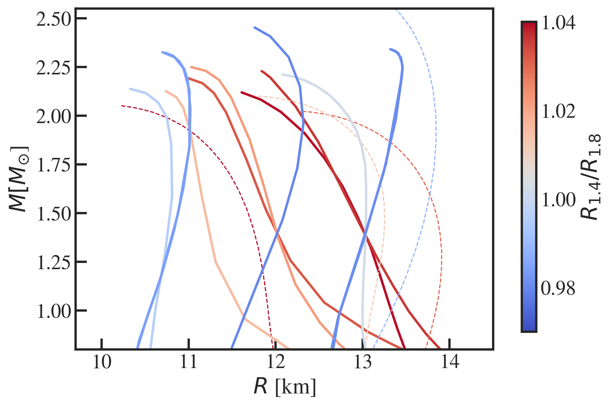
Figure 1: Mass-radius relations for the equations of state simulated in this work. The solid lines correspond to our parametric models, while the dashed line represent four commonly used finite-temperature EoS tables included in this work (in order of increasing radius, these are: SLy4, BHB$\Lambda\phi$, TMA for the red curves, and LS375 in blue). We color-code the curves according to $R_{1.4}/R_{1.8}$, where $R_{x}$ represents the radius of a star with mass $M=xM_{\odot}$. The parametric EoS sample (solid lines) is specifically constructed to sample a wide range of slopes in the mass-radius relations.

Different from previous works (e.g.,Takami et al. 2014; Vretinaris et al. 2020), our EoS sample spans a wide range of slopes in the mass-radius relation, with multiple EoSs that predict a backwards-bending mass-radius slopes. In particular, we construct families of EoSs that have an identical characteristic radius $R_{1.4}$, but that vary significantly in their radii at higher masses. This allows us, for the first time, to systematically investigate how the common set of quasi-universal relations for the post-merger GW frequency $f_{2}$ break down when the sample of EoS is significantly broadened.

In addition to these parametrically-constructed EoSs, we also simulate four existing, finite-temperature EoS tables: the nuclear EoS of Lattimer & Swesty (1991) with a bulk incompressibility of 375 MeV (“LS375”); the nuclear EoS SLy4 (Schneider et al., 2017) ; the nuclear EoS TMA (Toki et al., 1995; Hempel & Schaffner-Bielich, 2010) , and the hyperonic EoS BHB$\Lambda\phi$ (Banik et al., 2014) . With this comprehensive EoS sample, we can assess the validity of our findings for both commonly used and newly constructed EoS tables.

In order to investigate the impact of the different mass-radius slopes on the post-merger GW emission, we simulate the coalescence of a GW170817-like event for each of the fourteen EoSs in our sample. For our baseline simulations, we consider a moderate mass ratio of $q=0.85$ for a system with a total mass of $M=2.73\,M_{\odot}$. For a subset of models, we also perform simulations with the same chirp mass, but with $q=1$. For each EoS, we construct numerical initial conditions of compact binaries on quasi-circular orbits using the LORENE code (Gourgoulhon et al., 2001). We then use the Frankfurt-/IllinoisGRMHD (FIL) code (Most et al., 2019; Etienne et al., 2015) to solve the coupled Einstein-hydrodynamics system (Duez et al., 2005) using the Z4c formulation (Hilditch et al., 2013). FIL operates on top of the Einstein Toolkit infrastructure (Loffler et al., 2012; Schnetter et al., 2004). A detailed description of the numerical setup can be found in Most & Raithel (2021).

3 Results

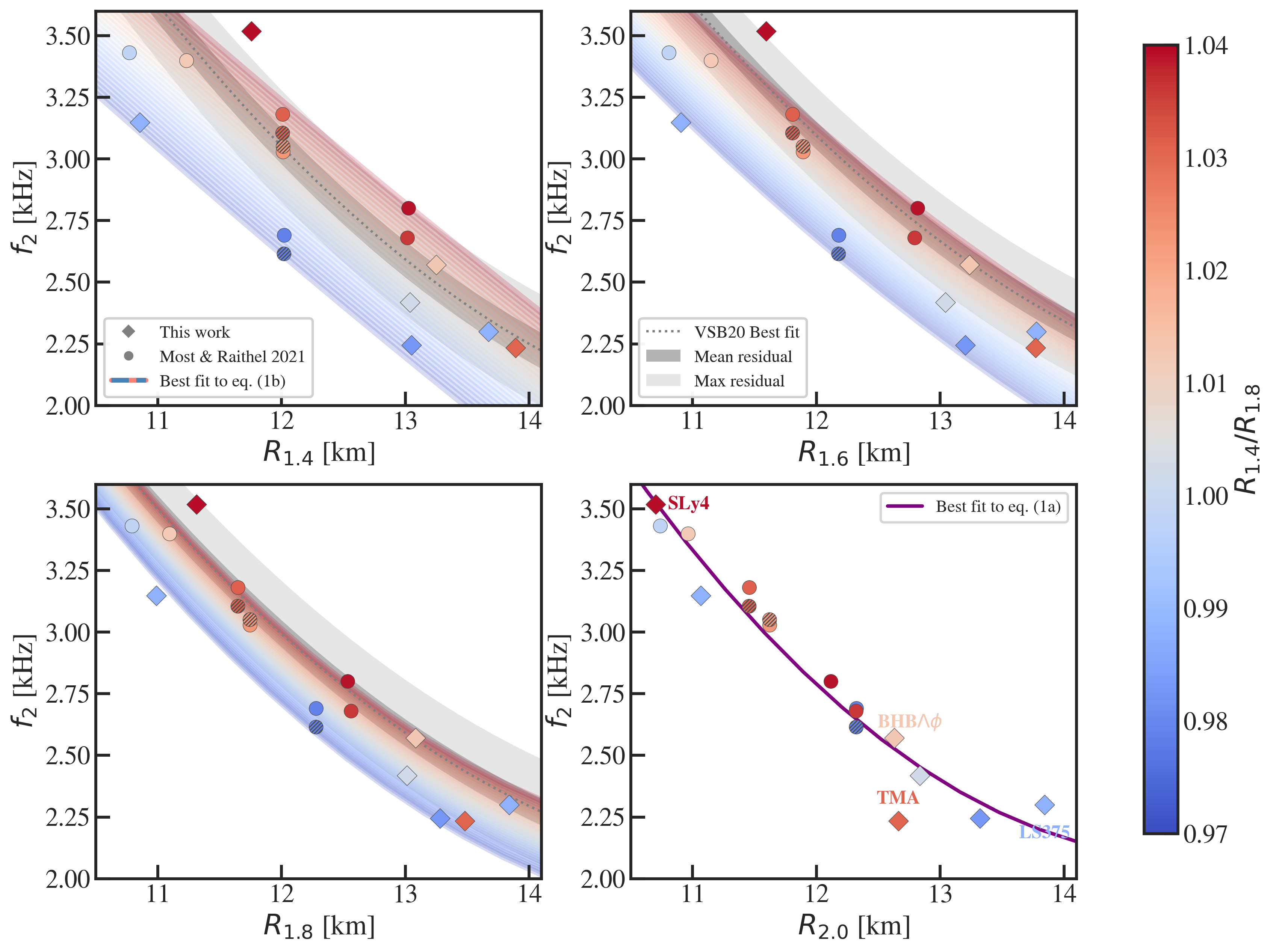
Figure 2: Peak frequency of the post-merger GW spectrum as a function of the neutron star radius at various masses. The color coding is the same as in Fig. 1. Diamonds represent results from the new simulations performed in this work, while circles correspond to results from Most & Raithel (2021). We note that the results from the four microphysical EoS tables are included in all four panels, but are only labeled in the bottom right panel for clarity. Solid-filled symbols indicate a binary mass ratio of $q=0.85$, while the hatched symbols are for $q=1$. The dotted gray lines correspond to the best-fit, quasi-universal relations reported in Vretinaris et al. (2020), with mean and maximum residuals from that work shown in the dark and light gray bands, respectively. Finally, the blue and red lines correspond to our best-fit, two-parameter quasi-universal relations (eq. 1b), with varying values of $R_{1.4}/R_{1.8}$; while the purple line corresponds to the best-fit, single-parameter relation for $f_{2}(R_{2.0})$. We find that models with $R_{1.4}/R_{1.8}<1$ (blue points) systematically violate the existing quasi-universal relations for stars of intermediate mass (top row) and instead follow a separate relation between $f_{2}$ and $R_{x}$.

In this section, we present the results of our numerical simulations. We focus exclusively on the quasi-universal behavior of the post-merger GW frequency spectrum. These are computed as outlined in Appendix C of Most & Raithel (2021). From these spectra, we identify $f_{2}$ as the frequency corresponding to the maximum power. We show $f_{2}$ as a function of the radius at various masses in Fig. 2, for each of the EoSs simulated in this work, as well as a previous set of simulations from Most & Raithel (2021).

Figure 2 also shows, for reference, the quasi-universal relations found in Vretinaris et al. (2020) between $f_{2}$ and $R_{1.4}$, $R_{1.6}$, and $R_{1.8}$. Correlations with $R_{2.0}$ were not studied in that work. The dashed gray line shows the best fit relations from Vretinaris et al. (2020), while the dark and light gray bands represent the mean and maximum residuals, respectively. Overall, we find a similar inverse correlation between $f_{2}$ and the radius at any mass, but one that is much broader than reported in Vretinaris et al. (2020). In particular, we find that a large number of our models violate the existing quasi-universal relations. For example, when considering the correlations with $R_{1.4}$ or $R_{1.6}$ (top row of Fig. 2), we find that 5-6 of the models fall outside of the previous maximum-residual error bands, and a majority fall outside of the mean-residual error band of Vretinaris et al. (2020). This violation of the quasi-universal relations is extreme, with $f_{2}$ varying by up to $\sim\,$600 Hz for models with the same characteristic $R_{1.4}$. The scatter is largest for the correlation with $R_{1.4}$, and decreases at increasing masses. Only when correlating $f_{2}$ as a function of $R_{1.8}$ do we find that most of our models fall within the previous maximum error band. However, even in this case, many of the EoSs populate the extreme lower edge of that error band.

In all three of these cases ($R_{1.4},\ R_{1.6}\,\ \text{and}\ R_{1.8}$), we find a strong trend between the degree to which the quasi-universal relations are violated and the slope of the mass-radius curve, which is here characterized by the ratio $R_{1.4}/R_{1.8}$ (for alternate definitions of the slope, see the discussion in the Appendix B). The models that most strongly violate the existing quasi-universal relations are those with $R_{1.4}/R_{1.8}<1$, which corresponds to the EoSs with a backwards-bending mass-radius relation in Fig. 1. This phenomenological $M-R$ behavior is caused by a stiffening of the EoS at high densities, such that more massive stars are characterized by steeper pressure gradients, and thus extend to larger radii. This type of behavior is consistent with the predictions, for example, of the emergence of a quarkyonic phase of matter (McLerran & Reddy, 2019). On the other hand, an EoS with significant softening at high densities (caused, e.g., by a cross-over phase transition) is characterized by a forwards-tilting $M-R$ relation, with decreasing radii at high masses. In general, we find that models with $R_{1.4}/R_{1.8}<1$ (EoSs with significant stiffening at high densities), lead to systematically lower values of $f_{2}$, while models with $R_{1.4}/R_{1.8}>1$ (EoSs with significant softening), lead to larger $f_{2}$. Indeed, the red and blue points in Fig. 2 appear to follow separate quasi-universal relationships between $f_{2}$ and $R_{x}$.

We note that the correlations for EoSs with forward-bending $M-R$ curves (red points) are still largely consistent with the existing quasi-universal relations. In the limit of extreme softening in the EoS (i.e., a first-order phase transition to a stable hybrid star), Bauswein et al. (2019) have shown that the $f_{2}$ quasi-universal relations can also be broken, and that this feature can be used to infer the presence of a phase transition from the post-merger GWs. The trend reported in that work is the same as we find in Fig. 2 – i.e., that EoSs with softening tend to have larger $f_{2}$ – but our family of EoSs with softening are less extreme (i.e., no first-order phase transitions) and thus show more modest violations in that direction.

We confirm that these trends between $f_{2}$ and the mass-radius slope are not very sensitive to the mass ratio of the binary by performing a subset of the simulations at a second mass ratio of $q=1$. These points (which correspond to the three models with $R_{1.4}=12$ km) are shown in Fig. 2 with hatched shading. We find small shifts in $f_{2}$ depending on the mass ratio, as has also been found in previous studies (e.g., Bernuzzi et al. 2015; Rezzolla & Takami 2016), but that the overall trend with $R_{1.4}/R_{1.8}$ is maintained.

In order to confirm that our results are robust to the parametric construction of the EoSs, we perform one further simulation with an approximate version of the TMA EoS, where the finite-temperature and composition-dependent dimensions of the EoS table have been replaced by the complete $M^{*}$-framework, using the TMA-specific parameters listed in Raithel et al. (2019). The peak frequency extracted with the parametric version of the EoS table is consistent with the $f_{2}$ obtained using the full table to within 20 Hz, thus confirming that the parametric thermal treatment produces reliable peak frequencies. A further comparison of $M^{*}$-parametric EoS to tabulated EoS in the context of merger simulations is presented in Raithel et al. (2022).

In addition, we find that the three microphysical EoS tables, SLy4, BHB$\Lambda\phi$, and LS375, all support the trend we have identified with the parametric EoSs. In particular, LS375 leads to a smaller-than-expected $f_{2}$, while SLy4 leads to a larger $f_{2}$ than predicted by the previous quasi-universal relations. Both of these deviations are explained by the mass-radius slopes of these EoSs. The peak frequency for BHB$\Lambda\phi$, which predicts only a small MR-slope, lies closer to the existing quasi-universal relation, also as expected. The peak frequency for TMA (the right-most red diamond in Fig. 2) is a modest outlier, which we attribute to the changing curvature of its mass-radius slope. We discuss this point further in Appendix B.

In order to quantify these trends with mass-radius slope, we fit the results shown in Fig. 2 to two different functional forms, using a standard, non-linear, least-squares fitting algorithm. The first functional form is a single-parameter relation motivated by the fits done in Vretinaris et al. (2020), which were quadratic in $R_{x}$ (where $x$ represents an arbitrary stellar mass). We also consider a two-parameter relation, which adds a linear correction term that scales with $R_{1.4}/R_{1.8}$, in order to account for the trends observed in Fig. 2. The fitting functions are thus

$$f_{2}(R_{x}) =b_{0}+b_{1}R_{x}+b_{2}R_{x}^{2}$$ (1a)

$$f_{2}(R_{x},\frac{R_{1.4}}{R_{1.8}}) =b_{0}+b_{1}R_{x}+b_{2}R_{x}^{2}+b_{3}\left(\frac{R_{1.4}}{R_{1.8}}\right),$$ (1b)

where $b_{i}~{}(i\in[0,3])$ are the fit coefficients. We note that we do not include the chirp mass as a free parameter (in contrast to Vretinaris et al. 2020) because all simulations done in this work are for a fixed $\mathcal{M}_{c}=1.186~{}M_{\odot}$. Thus, our fits can be viewed as characterizing one slice of the $f_{2}-R_{x}-\mathcal{M}_{c}$ plane that was identified in Vretinaris et al. (2020). The best-fit coefficients for eq. (1) are reported in Table 1, for various choices of $R_{x}$. To illustrate the performance of these fits, Fig. 2 additionally shows the best-fit, two-parameter relations for $R_{1.4}$ ,$R_{1.6}$ and $R_{1.8}$ with varying choices of the slope parameter (shown in the light blue-to-red shading), as well as the best-fit, single-parameter relation for $R_{2.0}$ (in purple). Finally, Table 1 also reports the adjusted coefficient of determination ($\mathcal{R}^{2}$) for each fit, the Bayesian Information Criteria (BIC), and the maximum and mean residuals.

Table 1: Fit coefficients for eqs. (1a) and (1b). All coefficients assume radii in km and $f_{2}$ in kHz. The right-most four columns contain the adjusted coefficient of determination ($\mathcal{R}^{2}$), the Bayesian information criterion, the maximum residual, and the mean residual for each fit. In this table, $R_{x}$ indicates the radius of a neutron star with mass $M=xM_{\odot}$, while $R_{\rm max}$ indicates the radius corresponding to the maximum mass configuration.

$R_{x}$	$b_{0}$	$b_{1}$	$b_{2}$	$b_{3}$	Adjusted $\mathcal{R}^{2}$	BIC	Max resid (kHz)	Mean resid (kHz)
$R_{1.4}$	1.754	0.573	-0.039	$-$	0.680	3.5	0.43	0.17
$R_{1.6}$	5.384	0.001	-0.017	$-$	0.793	-3.9	0.38	0.13
$R_{1.8}$	11.379	-0.964	0.022	$-$	0.883	-13.5	0.29	0.10
$R_{2.0}$	19.554	-2.328	0.078	$-$	0.932	-22.9	0.28	0.07
$R_{\rm max}$	21.740	-2.833	0.102	$-$	0.919	-19.9	0.22	0.09
$R_{1.4}$	0.081	-0.592	0.007	8.900	0.927	-20.2	0.21	0.08
$R_{1.6}$	5.403	-1.083	0.027	6.544	0.923	-19.3	0.21	0.08
$R_{1.8}$	12.179	-1.821	0.057	4.287	0.933	-21.7	0.20	0.07
$R_{2.0}$	19.455	-2.459	0.083	0.837	0.929	-20.6	0.30	0.07
$R_{\rm max}$	21.421	-2.871	0.104	0.504	0.913	-17.2	0.23	0.08

We turn first to the results of the single-parameter fits. The strength of the correlation between $f_{2}$ and $R_{x}$ increases significantly as we consider larger masses $x$, as expected based on the scatter seen in Fig. 2. For example, the adjusted $\mathcal{R}^{2}$ for the single-parameter fit to $R_{1.4}$ is only 0.68, but it increases to 0.93 for $R_{2.0}$. The $\Delta$BIC also shows strong evidence for each subsequently larger mass compared to the previous (e.g., $R_{1.8}$ is favored over $R_{1.6}$, etc.). The correlation is strongest for $R_{2.0}$. If we correlate instead with the radius corresponding to the maximum mass (as in, e.g., Bauswein & Janka 2012), the adjusted $\mathcal{R}^{2}$ decreases and the correlation is disfavored, compared to $R_{2.0}$.

When comparing the results of eq. (1a) and (1b) with our sample of EoSs, we find strong evidence in favor of adding this second parameter to the existing quasi-universal relations. For example, when comparing the evidence for a single-parameter fit with $R_{1.4}$ to the two-parameter fit with $R_{1.4}/R_{1.8}$, we find $\Delta$BIC$\approx 24$, indicating decisive evidence for the latter model. The results are similar for $R_{x}=R_{1.6}$ (“decisive” evidence with $\Delta$BIC=15) and $R_{1.8}$ (“strong” evidence with $\Delta$BIC=8). For the case of $R_{x}=R_{2.0}$, the correlation with the single-parameter fitting formula is already quite strong, and we do not find statistical evidence to justify the addition of a second parameter.

To summarize, we find that the existing, single-parameter quasi-universal relations all break down for EoSs with significant stiffening at high densities, i.e., with backwards-bending mass-radius relations. We find that for $R_{1.4}$, $R_{1.6}$, and $R_{1.8}$, the existing single-parameter relations are all significantly improved with the addition of a second parameter, which incorporates information about the $M-R$ slope. Indeed, by expanding the functional forms to include a second parameter ($R_{1.4}/R_{1.8}$), we are able to recover quasi-universality, as evidenced by coefficients of determination near unity. Alternatively, we are also able to better maintain quasi-universality for the correlation between $f_{2}$ and a single radius at sufficiently high masses, here for $R_{2.0}$.

The fact that quasi-universality is recovered for radii at very high masses strongly suggests that $f_{2}$ depends on the EoS at high densities. In addition, the slope of the $M-R$ relation has been shown to correlate with the pressure at $\sim 3.7\rho_{\rm sat}$ (Ozel & Psaltis, 2009), where $\rho_{\rm sat}\approx 2.7\times 10^{14}$ g/cm³ is the nuclear saturation density. Thus, by adding a slope-dependent parameter to the fitting function for $R_{x}$ at low masses, we are effectively adding in information about the high-density EoS, which also helps to restore the quasi-universality.

We note that for EoSs that predict mass-radius curves with significant curvature in their slopes, such as TMA, the choice of where to define a mass-radius slope is not always obvious. In this work, we use a definition of the slope that leads to the best goodness-of-fit statistics. We discuss alternate definitions of the slope and their (negligible) impact on our conclusions in Appendix B.

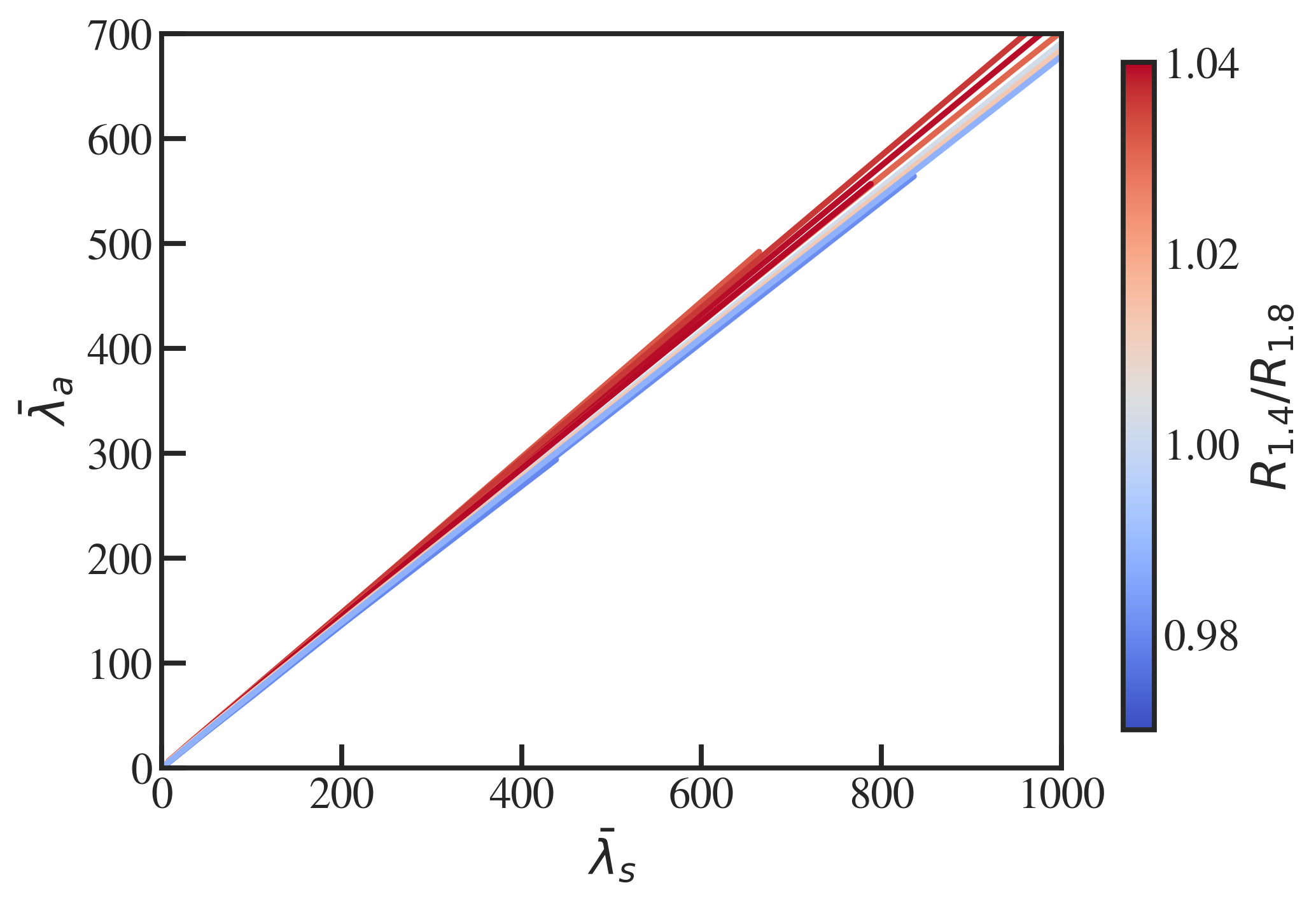
Figure 3: Binary Love relations for the symmetric $\bar{\lambda}_{s}$ and antisymmetric, $\bar{\lambda}_{a}$ tidal deformabilities of the coalescing binary with mass ratio $q=0.85$ considered in this work. Different curves correspond to the various equation of state models used, with color indicating the slope of the mass-radius curve in terms of the ratio $R_{1.4}/R_{1.8}$, where $R_{x}$ denotes the radius of a neutron star with mass $M=x\,M_{\odot}$.

4 Discussion and Conclusions

In this Letter, we have shown that the existing family of single-parameter, quasi-universal relations are insufficient to reliably infer the radius of an intermediate-mass neutron star from the post-merger GW frequencies alone. EoSs that produce backwards-bending mass-radius curves lead to systematically lower values of the post-merger peak frequencies $f_{2}$. As a result, we show that such EoSs violate existing quasi-universal relations proposed to infer neutron star radii, e.g., $R_{1.4}$, $R_{1.6}$, or $R_{1.8}$, from the post-merger frequency $f_{2}$. Moreover, we find that the EoSs that violate the existing relations form their own, separate quasi-universality class, which can be used to relate $f_{2}$ to neutron star radii for a fixed mass-radius slope (see Fig. 2). This observation motivates the extension of existing quasi-universal relations to incorporate a second parameter, related to the slope of the mass-radius curve. For the sample of EoSs explored in this Letter, we find strong statistical evidence in favor of the two-parameter, quasi-universal relations, compared to models that do not incorporate information about the mass-radius slope.

Interestingly, we find that single-parameter quasi-universality can be better maintained when considering massive neutron stars $M\simeq 2\,M_{\odot}$. Intuitively, this is consistent with the fact that the post-merger remnant itself is a massive neutron star, and thus probes higher densities than are present in the inspiral. Hence, we might reasonably expect that the peak frequencies of the post-merger GWs should correlate more strongly with parameters of the high-density EoS (this is also consistent with our findings in Most & Raithel 2021).

The better universality of the $f_{2}-R_{2.0}$ relation is of particular interest, given the recent NICER observations of the $\sim 2~{}M_{\odot}$ neutron star PSR J0740+6620, for which two recent radius inferences have been performed (Miller et al., 2021; Riley et al., 2021). Based on our findings, we expect that a future measurement of $f_{2}$ will be be able to provide robust and independent constraints on the radius of this pulsar.

If such a measurement of $R_{2.0}(f_{2})$ can be supplemented with constraints on $R_{1.4}$ from the inspiral measurement of the tidal deformability (see, e.g., Baiotti 2019; Raithel 2019; Chatziioannou 2020), then a sufficiently sensitive merger event – observed from inspiral through postmerger – could effectively be used to the trace out the entire mass-radius relation, to linear order.

Alternatively, it may also be possible to reconstruct the linearized mass-radius curve by utilizing the so-called binary Love relations of Yagi & Yunes (2016). These relations relate symmetric, $\bar{\lambda}_{s}=\frac{1}{2}\left(\bar{\lambda}_{1}+\bar{\lambda}_{2}\right)$, and antisymmetric, $\bar{\lambda}_{a}=\frac{1}{2}\left(\bar{\lambda}_{1}-\bar{\lambda}_{2}\right)$, combinations of the mass-normalized tidal deformabilities $\bar{\lambda}_{1,2}$ of the inspiralling neutron stars in an EoS-insensitive way (Yagi & Yunes, 2016). In a recent work, Tan et al. (2021) showed that these relations, previously thought to be fully universal, also receive an effective correction that is linearly proportional to the slope of the mass-radius curve. We illustrate this behavior in Fig. 3, where we show the $\bar{\lambda}_{a}-\bar{\lambda}_{s}$ correlation for the EoS and binary parameters used in this work. We can clearly see that, in line with Tan et al. (2021), there is a range of slopes separating EoSs with backwards- and forwards-bending mass-radius curves. Because the binary-Love relation also depends on the neutron star radius and mass-radius slope, but with a different dependence than our two-parameter, quasi-universal relations for $f_{2}$, combined detections of inspiral and post-merger should enable a reconstruction of the linearized mass-radius curve.

While our findings constitute strong evidence for the existence of a two-parameter, quasi-universal relation for $f_{2}(R_{x},R_{1.4}/R_{1.8}$) in our sample, future work will be necessary to further quantify this new dependency on the mass-radius slope. In particular, this will require a systematic investigation of an even larger number of EoSs with varying and non-linear mass-radius slopes, and simulations of a wide class of binary masses and mass ratios. We leave such detailed explorations to future work.

Appendix A New piecewise polytropic EoS models studied in this work

In this appendix, we provide additional details on the new piecewise polytropic EoSs constructed for this work. As described in Sec. 2, seven of the ten piecewise polytropic EoSs studied in this work were previously presented in Most & Raithel (2021), and we refer the reader to that paper for details on those models. We show the three new models, which were constructed specifically for this study, in Fig. 4. These models correspond to some of the most extreme backwards-bending mass-radius relations from Fig. 1. As can be seen in Fig. 4, the backwards-bending phenomenology is produced by a stiffening of the EoS at intermediate densities.

As was the case for the original sample of seven EoSs constructed in Most & Raithel (2021), these three new models are subject to several physical constraints. In particular, we require that each of these EoSs remain causal and thermodynamically stable, and that the maximum mass of each EoS is at least 2 $M_{\odot}$, in order to be consistent with the observation of massive pulsars (Demorest et al., 2010; Antoniadis et al., 2013; Fonseca et al., 2016; Cromartie et al., 2019). In addition, we impose a lower limit on the pressure at our first fiducial density $P(0.86~{}\rho_{\rm sat})\gtrsim 1.7\times 10^{33}\text{dyn/cm}^{2}$, which is set by the two-body potential of Argonne AV8 (Gandolfi et al., 2014).

The radii and tidal deformabilities of these EoS models are presented in Table 2. In addition, Table 2 also reports the piecewise polytropic parameters that describe each EoS. We note that all of the phenomenological EoS models used in this work comprise five piecewise polytropic segments, which are spaced log-uniformly in the density. The fixed dividing densities are located at [0.86, 1.47, 2.52, 4.32, and 7.4] $\times\rho_{\rm sat}$, where $\rho_{\rm sat}=2.7\times 10^{14}\text{g/cm}^{3}$ is the nuclear saturation density. As described in Sec. 2, the EoS is fixed at densities below $0.5\rho_{\rm sat}$ to SFHo. We list this anchoring pressure as well in Table 2 for convenience. For details on constructing piecewise polytropic EoSs using these parameters, see, e.g. Read et al. (2009); Ozel & Psaltis (2009); Raithel et al. (2016).

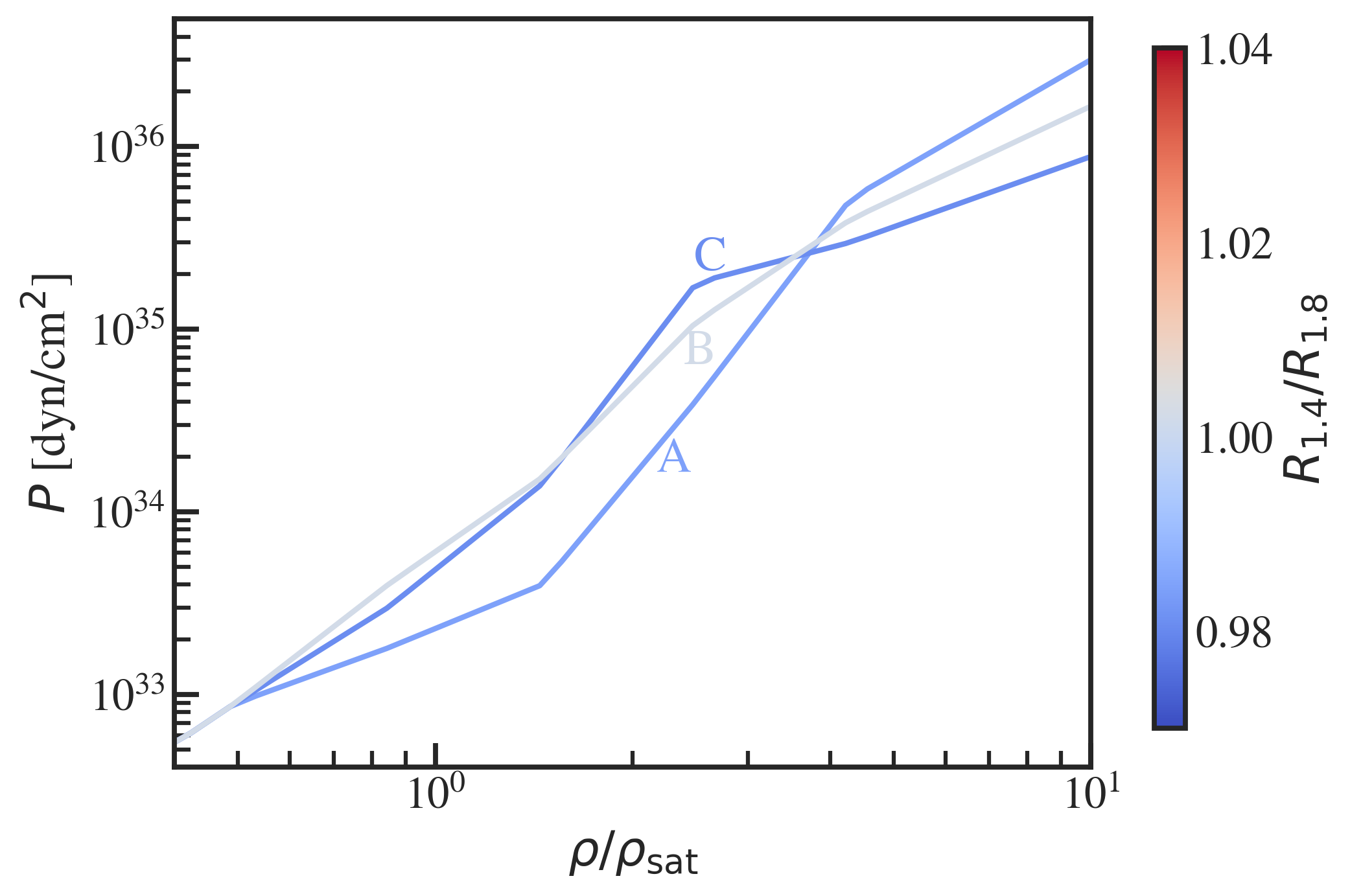
Figure 4: Pressure as a function of density for the three piecewise-polytropic EoSs newly constructed in this work. The density, $\rho$, is plotted with respect to the nuclear saturation density, $\rho_{\rm sat}=2.7\times 10^{14}\text{g/cm}^{3}$. The labels are arbitrarily assigned, for reference in Table 2.

Table 2: Parameters describing the three new piecewise, polytropic EoSs considered in this work. The first column gives the model labels from Fig. 4. The second and third columns report the radius and tidal deformability of a 1.4 $M_{\odot}$ neutron star, respectively. The remaining columns report the pressures at each fiducial density in the piecewise polytropic model. All pressures are given in units of dyn/cm².

Model	$R_{1.4}$ (km)	$\Lambda_{1.4}$	$P(0.5\rho_{\rm sat})$	$P(0.86\rho_{\rm sat})$	$P(1.47\rho_{\rm sat})$	$P(2.52\rho_{\rm sat})$	$P(4.32\rho_{\rm sat})$	$P(7.4\rho_{\rm sat})$
A	10.8	216	8.88$\times 10^{32}$	1.80$\times 10^{33}$	4.00$\times 10^{33}$	4.10$\times 10^{34}$	5.20$\times 10^{35}$	1.60$\times 10^{36}$
B	13.0	608	8.88$\times 10^{32}$	4.00$\times 10^{33}$	1.55$\times 10^{34}$	1.10$\times 10^{35}$	4.00$\times 10^{35}$	1.00$\times 10^{36}$
C	13.0	665	8.88$\times 10^{32}$	3.10$\times 10^{33}$	1.43$\times 10^{34}$	1.80$\times 10^{35}$	3.00$\times 10^{35}$	6.00$\times 10^{35}$

Appendix B Alternate definitions of the mass-radius slope

Table 3: Fit coefficients for eq. (1b) for alternate definitions of the mass-radius slope. The formatting is otherwise identical to Table 1. The results with the slope parameter $R_{1.4}/R_{1.8}$ are repeated for reference.

Slope	$R_{x}$	$b_{0}$	$b_{1}$	$b_{2}$	$b_{3}$	Adjusted $\mathcal{R}^{2}$	BIC	Max resid (kHz)	Mean resid (kHz)
	$R_{1.4}$	0.081	-0.592	0.007	8.900	0.927	-20.2	0.21	0.08
	$R_{1.6}$	5.403	-1.083	0.027	6.544	0.923	-19.3	0.21	0.08
$R_{1.4}/R_{1.8}$	$R_{1.8}$	12.179	-1.821	0.057	4.287	0.933	-21.7	0.20	0.07
	$R_{2.0}$	19.455	-2.459	0.083	0.837	0.929	-20.6	0.30	0.07
	$R_{\rm max}$	21.421	-2.871	0.104	0.504	0.913	-17.2	0.23	0.08
	$R_{1.4}$	16.073	-1.780	0.057	-0.204	0.848	-7.7	0.44	0.10
	$R_{1.6}$	16.180	-1.792	0.057	-0.148	0.874	-10.9	0.39	0.09
$\frac{\partial R}{\partial M}\biggr{\rvert}_{1.2}$	$R_{1.8}$	18.674	-2.191	0.073	-0.102	0.918	-18.1	0.28	0.08
	$R_{2.0}$	22.530	-2.848	0.100	-0.066	0.946	-25.2	0.27	0.06
	$R_{\rm max}$	23.182	-3.112	0.116	-0.070	0.937	-22.7	0.21	0.07
	$R_{1.4}$	10.058	-0.790	0.016	-0.244	0.880	-11.7	0.34	0.09
	$R_{1.6}$	12.202	-1.139	0.030	-0.177	0.889	-13.0	0.33	0.09
$\frac{\partial R}{\partial M}\biggr{\rvert}_{1.4}$	$R_{1.8}$	16.467	-1.828	0.058	-0.118	0.919	-18.4	0.25	0.08
	$R_{2.0}$	21.120	-2.606	0.090	-0.049	0.934	-21.8	0.29	0.06
	$R_{\rm max}$	22.746	-3.030	0.112	-0.057	0.923	-19.3	0.24	0.08
	$R_{1.4}$	7.552	-0.365	-0.002	-0.283	0.910	-16.6	0.23	0.08
	$R_{1.6}$	11.070	-0.944	0.022	-0.206	0.910	-16.6	0.25	0.08
$\frac{\partial R}{\partial M}\biggr{\rvert}_{1.6}$	$R_{1.8}$	16.052	-1.755	0.055	-0.133	0.925	-19.7	0.20	0.07
	$R_{2.0}$	20.285	-2.457	0.083	-0.025	0.928	-20.4	0.30	0.07
	$R_{\rm max}$	21.976	-2.880	0.105	-0.017	0.913	-17.2	0.23	0.08

In this Letter, we have shown that the existing family of single-parameter, quasi-universal relations between $f_{2}$ and the neutron star radius break down for EoSs that predict non-vertical slopes in their mass-radius relations, but that universality may be restored by adding in a second parameter that depends on the slope. In this appendix, we confirm that this conclusion is robust to different definitions of the slope, including the value of $\partial R/\partial M$ evaluated at either 1.2, 1.4, or 1.6 $M_{\odot}$. We report the statistics for these fits in Table 3.

In particular, for each of these alternate definitions of the slope, there is still strong evidence in favor of adding a second parameter to the relationship between $f_{2}$ and $R_{1.4}$,$R_{1.6}$, or $R_{1.8}$ ($\Delta$ BIC $\gtrsim$ 5, compared to the mono-parametric fits reported in Table 1). As was found in the main text, for each these definitions the evidence favoring a second parameter again decreases as $f_{2}$ is correlated with radii at increasingly large masses, such that for $f_{2}(R_{2.0})$, there is no significant evidence in favor of adding a second parameter. This confirms that the conclusions of the main Letter do not change depending on where the slope is defined.

However, in spite of these qualitatively consistent trends, the goodness of fit does change slightly depending on the definition of the slope parameter. For example, in the fit for $f_{2}(R_{1.4},R_{1.4}/R_{1.8})$ reported in the main text, the adjusted $\mathcal{R}^{2}$ was 0.927. For $f_{2}(R_{1.4},\partial R/\partial M)$, the adjusted $\mathcal{R}^{2}$ value is reduced, ranging from 0.85 to 0.91, depending on the mass at which the slope is evaluated.

We find that the sensitivity to the definition of the mass-radius slope comes primarily from a subset of models, as can be seen in Fig. 5. Figure 5 shows the same set of EoSs from Fig. 1, but now color-coded by a local (or instantaneous) slope. The models have been divided into three panels for visual clarity, with forwards-tilting MR curves in the left panel, backwards-bending models in the middle panel, and models with varying mass-radius slope in the right panel. While the majority of curves can be well represented by a single slope parameter acorss the mass range of interest, a subset of models (grouped in the right panel of Fig. 5) show some degree of curvature in their mass-radius relations. These include the finite-temperature EoSs BHB$\Lambda\phi$ and TMA, as well as two of the parametric models. As a result, the goodness-of-fit for the quasi-universal relation relating $f_{2}$ to a characteristic radius and the mass-radius slope can be sensitive to where, precisely, the slope is defined.

In summary, we find that the main conclusions of this Letter are robust to these alternate definitions of the slope. However, for broader families of EoSs, it may be necessary to revisit this definition, or even to include additional correction terms to the quasi-universal relations that describe the shape of the mass-radius relation at beyond linear order. Understanding this dependence will require additional simulations, spanning a wide range of both linear and curved mass-radius relations, which expands the dimensionality of the problem significantly. We leave such an investigation to a future study.

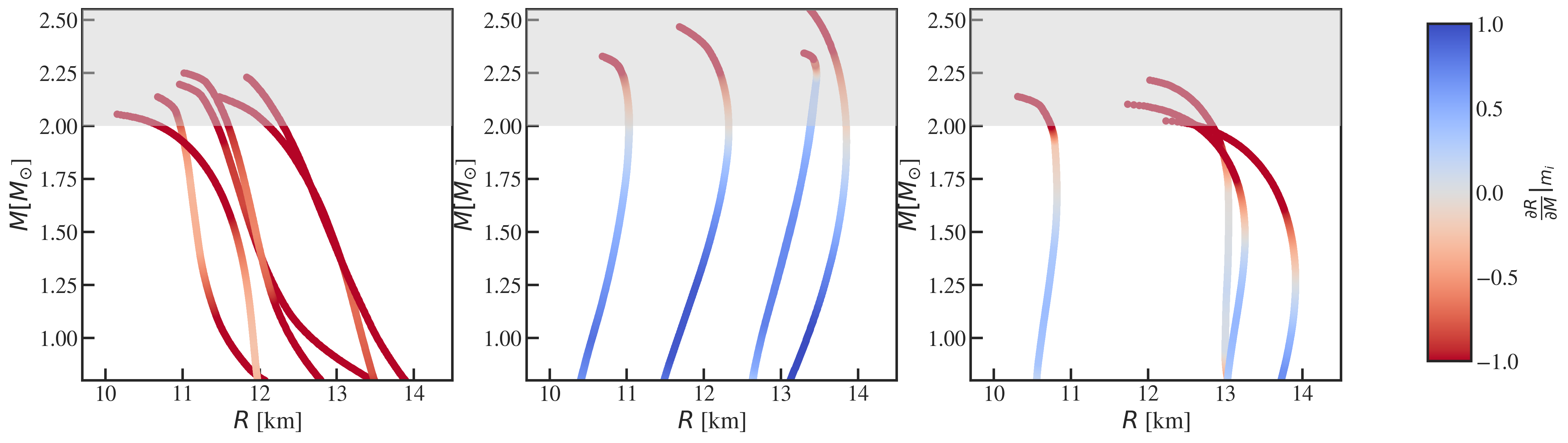
Figure 5: Mass-radius relation for the same set of EoSs shown in Fig. 1, but now color-coded according to the instantaneous slope. The models have been divided into three panels for visual clarity. Masses above 2 $M_{\odot}$ have been grayed out because the mass-radius curves of all EoSs turn-over near the maximum mass, and so the changing slope in this mass range is not especially interesting. Focusing instead then on the mass range of 1-2 $M_{\odot}$, it is clear that the majority of these curves can be well defined by a single slope parameter; however, for a subset of cases (grouped in the right-most panel), the slope is sensitive to the mass at which it is defined.

References

- Abbott et al. (2017) Abbott, B. P., et al. 2017, Phys. Rev. Lett., 119, 161101
- Antoniadis et al. (2013) Antoniadis, J., et al. 2013, Science, 340, 6131
- Baiotti (2019) Baiotti, L. 2019, Prog. Part. Nucl. Phys., 109, 103714
- Baiotti & Rezzolla (2017) Baiotti, L., & Rezzolla, L. 2017, Rept. Prog. Phys., 80, 096901
- Banik et al. (2014) Banik, S., Hempel, M., & Bandyopadhyay, D. 2014, Astrophys. J. Suppl., 214, 22
- Bauswein et al. (2019) Bauswein, A., Bastian, N.-U. F., Blaschke, D. B., et al. 2019, Phys. Rev. Lett., 122, 061102
- Bauswein & Janka (2012) Bauswein, A., & Janka, H. T. 2012, Phys. Rev. Lett., 108, 011101
- Bauswein et al. (2012) Bauswein, A., Janka, H. T., Hebeler, K., & Schwenk, A. 2012, Phys. Rev. D, 86, 063001
- Bauswein & Stergioulas (2019) Bauswein, A., & Stergioulas, N. 2019, J. Phys. G, 46, 113002
- Bernuzzi (2020) Bernuzzi, S. 2020, Gen. Rel. Grav., 52, 108
- Bernuzzi et al. (2015) Bernuzzi, S., Dietrich, T., & Nagar, A. 2015, Phys. Rev. Lett., 115, 091101
- Chatziioannou (2020) Chatziioannou, K. 2020, Gen. Rel. Grav., 52, 109
- Cromartie et al. (2019) Cromartie, H. T., et al. 2019, Nature Astron., 4, 72
- Demorest et al. (2010) Demorest, P., Pennucci, T., Ransom, S., Roberts, M., & Hessels, J. 2010, Nature, 467, 1081
- Duez et al. (2005) Duez, M. D., Liu, Y. T., Shapiro, S. L., & Stephens, B. C. 2005, Phys. Rev. D, 72, 024028
- Etienne et al. (2015) Etienne, Z. B., Paschalidis, V., Haas, R., Mösta, P., & Shapiro, S. L. 2015, Class. Quant. Grav., 32, 175009
- Fonseca et al. (2016) Fonseca, E., et al. 2016, Astrophys. J., 832, 167
- Gandolfi et al. (2014) Gandolfi, S., Carlson, J., Reddy, S., Steiner, A. W., & Wiringa, R. B. 2014, Eur. Phys. J. A, 50, 10
- Gourgoulhon et al. (2001) Gourgoulhon, E., Grandclement, P., Taniguchi, K., Marck, J.-A., & Bonazzola, S. 2001, Phys. Rev. D, 63, 064029
- Guerra Chaves & Hinderer (2019) Guerra Chaves, A., & Hinderer, T. 2019, J. Phys. G, 46, 123002
- Hempel & Schaffner-Bielich (2010) Hempel, M., & Schaffner-Bielich, J. 2010, Nucl. Phys. A, 837, 210
- Hilditch et al. (2013) Hilditch, D., Bernuzzi, S., Thierfelder, M., et al. 2013, Phys. Rev. D, 88, 084057
- Hunter (2007) Hunter, J. D. 2007, Computing in Science & Engineering, 9, 90
- Jeffreys (1961) Jeffreys, H. 1961, Theory of Probability, 3rd edn. (Oxford, England: Oxford)
- Lattimer & Swesty (1991) Lattimer, J. M., & Swesty, F. D. 1991, Nucl. Phys. A, 535, 331
- Liddle (2007) Liddle, A. R. 2007, Mon. Not. Roy. Astron. Soc., 377, L74
- Loffler et al. (2012) Loffler, F., et al. 2012, Class. Quant. Grav., 29, 115001
- McLerran & Reddy (2019) McLerran, L., & Reddy, S. 2019, Phys. Rev. Lett., 122, 122701
- Miller et al. (2021) Miller, M. C., et al. 2021, Astrophys. J. Lett., 918, L28
- Most et al. (2019) Most, E. R., Papenfort, L. J., & Rezzolla, L. 2019, Mon. Not. Roy. Astron. Soc., 490, 3588
- Most & Raithel (2021) Most, E. R., & Raithel, C. A. 2021, Phys. Rev. D, 104, 124012
- Özel & Freire (2016) Özel, F., & Freire, P. 2016, Ann. Rev. Astron. Astrophys., 54, 401
- Ozel & Psaltis (2009) Ozel, F., & Psaltis, D. 2009, Phys. Rev. D, 80, 103003
- Ozel et al. (2016) Ozel, F., Psaltis, D., Guver, T., et al. 2016, Astrophys. J., 820, 28
- Paschalidis & Stergioulas (2017) Paschalidis, V., & Stergioulas, N. 2017, Living Rev. Rel., 20, 7
- Raaijmakers et al. (2021) Raaijmakers, G., Greif, S. K., Hebeler, K., et al. 2021, Astrophys. J. Lett., 918, L29
- Radice et al. (2020) Radice, D., Bernuzzi, S., & Perego, A. 2020, Ann. Rev. Nucl. Part. Sci., 70, 95
- Raithel et al. (2022) Raithel, C., Espino, P., & Paschalidis, V. 2022, arXiv:2206.14838 [astro-ph.HE]
- Raithel (2019) Raithel, C. A. 2019, Eur. Phys. J. A, 55, 80
- Raithel et al. (2016) Raithel, C. A., Ozel, F., & Psaltis, D. 2016, Astrophys. J., 831, 44
- Raithel et al. (2017) Raithel, C. A., Özel, F., & Psaltis, D. 2017, Astrophys. J., 844, 156
- Raithel et al. (2019) Raithel, C. A., Ozel, F., & Psaltis, D. 2019, Astrophys. J., 875, 12
- Read et al. (2009) Read, J. S., Lackey, B. D., Owen, B. J., & Friedman, J. L. 2009, Phys. Rev. D, 79, 124032
- Rezzolla & Takami (2016) Rezzolla, L., & Takami, K. 2016, Phys. Rev. D, 93, 124051
- Riley et al. (2021) Riley, T. E., et al. 2021, Astrophys. J. Lett., 918, L27
- Schneider et al. (2017) Schneider, A. S., Roberts, L. F., & Ott, C. D. 2017, Phys. Rev. C, 96, 065802
- Schnetter et al. (2004) Schnetter, E., Hawley, S. H., & Hawke, I. 2004, Class. Quant. Grav., 21, 1465
- Steiner et al. (2013) Steiner, A. W., Hempel, M., & Fischer, T. 2013, Astrophys. J., 774, 17
- Steiner et al. (2010) Steiner, A. W., Lattimer, J. M., & Brown, E. F. 2010, Astrophys. J., 722, 33
- Steiner et al. (2016) —. 2016, Eur. Phys. J. A, 52, 18
- Stergioulas et al. (2011) Stergioulas, N., Bauswein, A., Zagkouris, K., & Janka, H.-T. 2011, Mon. Not. Roy. Astron. Soc., 418, 427
- Takami et al. (2014) Takami, K., Rezzolla, L., & Baiotti, L. 2014, Phys. Rev. Lett., 113, 091104
- Takami et al. (2015) —. 2015, Phys. Rev. D, 91, 064001
- Tan et al. (2021) Tan, H., Dexheimer, V., Noronha-Hostler, J., & Yunes, N. 2021, arXiv:2111.10260 [astro-ph.HE]
- Toki et al. (1995) Toki, H., Hirata, D., Sugahara, Y., Sumiyoshi, K., & Tanihata, I. 1995, Nucl. Phys. A, 588, c357
- Torres-Rivas et al. (2019) Torres-Rivas, A., Chatziioannou, K., Bauswein, A., & Clark, J. A. 2019, Phys. Rev. D, 99, 044014
- Vretinaris et al. (2020) Vretinaris, S., Stergioulas, N., & Bauswein, A. 2020, Phys. Rev. D, 101, 084039
- Waskom (2021) Waskom, M. L. 2021, Journal of Open Source Software, 6, 3021
- Yagi & Yunes (2016) Yagi, K., & Yunes, N. 2016, Class. Quant. Grav., 33, 13LT01