Impact of the nuclear symmetry energy on the post-merger phase of a binary neutron star coalescence

Abstract

The nuclear symmetry energy plays a key role in determining the equation of state of dense, neutron-rich matter, which governs the properties of both terrestrial nuclear matter as well as astrophysical neutron stars. A recent measurement of the neutron skin thickness from the PREX collaboration has lead to new constraints on the slope of the nuclear symmetry energy, $L$, which can be directly compared to inferences from gravitational-wave observations of the first binary neutron star merger inspiral, GW170817 In this paper, we explore a new regime for potentially constraining the slope, $L$, of the nuclear symmetry energy with future gravitational wave events: the post-merger phase a binary neutron star coalescence. In particular, we go beyond the inspiral phase, where imprints of the slope parameter $L$ may be inferred from measurements of the tidal deformability, to consider imprints on the post-merger dynamics, gravitational wave emission, and dynamical mass ejection. To this end, we perform a set of targeted neutron star merger simulations in full general relativity using new finite-temperature equations of state, which systematically vary $L$. We find that the post-merger dynamics and gravitational wave emission are mostly insensitive to the slope of the nuclear symmetry energy. In contrast, we find that dynamical mass ejection contains a weak imprint of $L$, with large values of $L$ leading to systematically enhanced ejecta.

I Introduction

Determining the equation of state (EoS) of dense, neutron-rich matter is a common goal in both modern nuclear physics and astrophysics. One of the key ingredients to the neutron-rich EoS is the nuclear symmetry energy, which characterizes the difference in energy between symmetric nuclear matter and pure neutron matter. The symmetry energy is often represented as a series expansion in density, with leading-order coefficients related to the value of the symmetry energy at the nuclear saturation density, $S$, and its slope, $L$, according to

$$E_{\rm sym}(n)=S+\frac{L}{3}\left(\frac{n}{n_{\rm sat}}-1\right)+\mathcal{O}\left[\left(\frac{n}{n_{\rm sat}}-1\right)\right]^{2}$$ (1)

where $n_{\rm sat}=0.16$ fm^-3 is the nuclear saturation density Piekarewicz and Centelles (2009).

A wide range of experimental efforts have placed constraints on $S$ and $L$, including from fits to nuclear masses, measurements of the giant dipole resonance and electric dipole polarizability of ²⁰⁸Pb, and observations of isospin diffusion or multifragmentation in heavy ion collisions (Tsang et al., 2012; Lattimer and Lim, 2013; Oertel et al., 2017). Recently, the Lead Radius Experiment (PREX-II) reported new constraints on the neutron radius of ²⁰⁸Pb which, when combined with results from the original PREX-I experiment Abrahamyan et al. (2012); Horowitz et al. (2012), imply a neutron skin thickness of $R_{\rm skin}^{{}^{208}\rm{Pb}}=0.283\pm 0.071$ fm Adhikari et al. (2021). From this measurement, Ref. Reed et al. (2021) constrained the slope of the symmetry energy to $L=106\pm 37$ MeV, which is larger than many previous constraints from microscopic calculations or experimental measurements Tsang et al. (2012); Lattimer and Lim (2013); Oertel et al. (2017); Li et al. (2021).

Following this new measurement of $L$, several studies have recently investigated its impact on the neutron star EoS. Neutron stars, which contain neutron-rich matter and probe densities around and above the nuclear saturation density, are an ideal laboratory for studying the symmetry energy. It has long been known that the slope of the symmetry energy correlates strongly with neutron star radius (Lattimer and Prakash (2001), see also Fig. 1). The radius in turn correlates with the neutron star tidal deformability Yagi and Yunes (2013, 2016); De et al. (2018); Raithel et al. (2018). Perhaps not surprisingly then, $L$ can also affect the gravitational wave emission during a binary neutron star inspiral (e.g., Fattoyev et al. (2014)). Measurements of these astrophysical quantities can thus, in principle, provide constraints on $L$ that are complementary to those inferred from laboratory-based experiments.

To illustrate this behavior, we show the inter-correlations between $R_{1.4}$, $\Lambda_{1.4}$, and the slope of the symmetry energy in Fig. 1, where $R_{1.4}$ and $\Lambda_{1.4}$ are the characteristic radius and tidal deformability of a 1.4 $M_{\odot}$ neutron star, respectively. Figure 1 was generated from a large sample of piecewise polytropic EoSs, which were constructed to uniformly sample the pressure at densities above half of the nuclear saturation density (see Sec. II.1 and Ref. Raithel et al. (2016) for further details). Figure 1 shows that, although $R_{1.4}$ and $\Lambda_{1.4}$ are indeed well correlated, there is significant scatter in the relationship, which depends sensitively on the value of $L$ in an approximately monotonic fashion. For example, for fixed values of $\Lambda_{1.4}\lesssim 500$, the corresponding value of $R_{1.4}$ can vary by nearly a kilometer, with $L$ likewise varying from $\lesssim 40$ MeV to more than 100 MeV. While these correlations hold for the radii of intermediate mass stars, the dependence on $L$ breaks down for higher-mass stars ($M>1.8~{}M_{\odot}$), which are governed less strongly governed by saturation physics Alam et al. (2016).

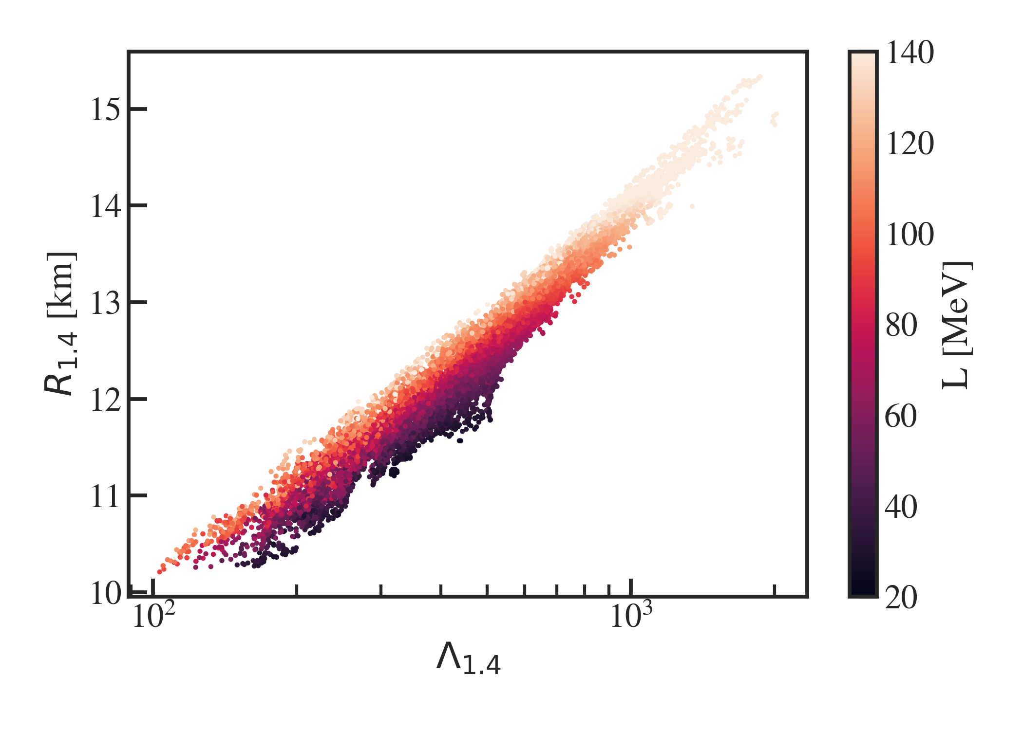
Figure 1: Correlations between $R_{1.4}$ and $\Lambda_{1.4}$ for a sample of $>10,000$ piecewise polytropic EoSs. Each EoS has five polytropic segments, spaced log-uniformly in density between 0.5 and 7.4$n_{\rm sat}$, with uniformly-drawn pressures. All EoSs support a maximum mass of at least 1.97 $M_{\odot}$. The symmetry energy slope is extracted according to eq. (6). We find that, although $R_{1.4}$ and $\Lambda_{1.4}$ are well correlated, there is a significant scatter in the trend, which depends approximately monotonically on the value of $L$.

Taking advantage of the types of correlations shown in Fig. 1, as well as correlations between $\Lambda_{1.4}$ and the higher-order symmetry energy coefficients, many studies have used the measurement of the tidal deformability from GW170817 Abbott et al. (2017a, 2019a) to derive new constraints on the nuclear symmetry energy Krastev and Li (2019); Malik et al. (2018); Carson et al. (2019); Raithel and Ozel (2019); Zhang and Li (2019); Tsang et al. (2019). For example, Ref. Raithel and Ozel (2019) demonstrated that, for a mono-parametric family of EoSs, GW170817 implies small values of $9\lesssim L\lesssim 65$ MeV. In a recent study combining astrophysical data from GW170817, NICER, and the existence of massive pulsars, together with theoretical constraints from chiral effective field theory, Ref. Essick et al. (2021) confirmed that the astrophysically-inferred slope of the symmetry energy ($L=52\begin{subarray}{c}+20\\ -18\end{subarray}$ MeV) is in mild tension with the PREX-II result. For a recent review on the status of astrophysical and laboratory constraints on the symmetry energy in light of GW170817 and the PREX-II experiment, see Li et al. (2021).

In this work, we explore a new regime for probing the nuclear symmetry energy: the post-merger phase of a binary neutron star merger. The post-merger phase probes higher densities and larger temperatures ($T>40\,\rm MeV$) than in the inspiral. As a result, astrophysical observables of the post-merger phase provide an ideal laboratory for probing the properties of hot, dense matter. For example, the gravitational waves (GWs) emitted by the post-merger remnant are expected to be a sensitive probe of the underlying cold EoS Baiotti and Rezzolla (2017); Paschalidis and Stergioulas (2017); Bauswein and Stergioulas (2019); Bernuzzi (2020); Radice et al. (2020), with additional corrections from the finite-temperature part of the EoS Bauswein et al. (2010); Raithel et al. (2021). The dynamics of the post-merger phase will also influence the quantity, velocity, and composition of the dynamical ejecta , which can in turn influence the associated kilonova, if detectable Metzger (2020); Radice et al. (2018); Kawaguchi et al. (2019); Shibata and Hotokezaka (2019). Modeling all of these effects requires accurate numerical relativity simulations of the post-merger phase that account for all relevant physical processes, including weak-interactions and finite temperature effects, see e.g. Radice et al. (2020) for a recent review.

Whereas most early studies resorted to ideal-fluid descriptions for the finite temperature part of the EoS and neglected nuclear composition entirely, many recent studies have instead made use of a limited number of publicly available EoS tables that enable self-consistent finite-temperature effects and out-of-(weak) equilibrium composition effects. One drawback of the latter approach, however, is the relatively small sample of available models, which can vary from one another in multiple nuclear parameters simultaneously, rendering systematic studies of the impact of individual nuclear parameters on merger simulations nearly impossible.

In this work, we take a third approach, enabled by a recently-developed framework for extending arbitrary cold EoSs to finite-temperatures and arbitrary compositions. The finite-temperature part of this EoS framework utilizes a Fermi Liquid Theory approach for including the leading-order effects of degeneracy, while the extrapolation to non-equilibrium compositions is based on a parametrization of the nuclear symmetry energy Raithel et al. (2019). The ability of this framework to model finite-temperature effects in neutron star merger simulations was recently explored by Ref. Raithel et al. (2021). In summary, this framework allows for the construction of new parametric, finite-temperature EoSs, which are ideally suited for systematic investigations of EoS imprints in neutron star mergers.

In particular, many previous studies have found that the post-merger GW emission or mass ejecta depend on the characteristic radius or tidal deformability of the underlying EoS Baiotti and Rezzolla (2017); Paschalidis and Stergioulas (2017); Radice et al. (2018); Bauswein and Stergioulas (2019); Shibata and Hotokezaka (2019); Bernuzzi (2020); Radice et al. (2020). These interconnected dependencies typically would make it difficult to disentangle variations in these macroscopic properties from any variations in the nuclear model, e.g., in $L$. To start to resolve this problem, in this work, we explicitly construct a set of seven new EoS models that fix $R_{1.4}$ or $\Lambda_{1.4}$, while systematically varying in $L$. In this way, we aim to disentangle the role of these macroscopic properties from the possible role of $L$ in determining the post-merger observables.

To further restrict the comparison of the EOSs to the supranuclear part, where $L$ plays a role, we construct each EoS to have an identical finite-temperature component and to follow the same tabulated EoS at densities below half of the nuclear saturation density (SFHo, Steiner et al. (2013a)). In this way, we ensure that the only difference in these new EoSs is in the cold physics at supranuclear densities, while also capturing low density effects, such as the formation of bound nuclei, by using a tabulated nuclear model.

In order to study the role of $L$ in the post-merger phase, we perform numerical simulations of binary neutron star mergers in full general relativity using each of these new EoSs. Our simulations follow the last few orbits of the binary inspiral, and continue through the merger and until $\sim$25 ms post-merger. We use these simulations to explore, in particular, the post-merger dynamics, post-merger gravitational wave emission, and dynamical mass ejection. We find that the slope $L$ of the symmetry energy does not leave clear imprints in the post-merger dynamics or GW emission, but rather find that these processes depend more sensitively on the high-density part of the EoS. In contrast, we find some first indication that the amount of dynamically ejected material correlates with the slope of the symmetry energy, with large values of $L$ leading to the production of significantly more dynamical ejecta. These links between $L$ and the ejecta may affect aspects of the electromagnetic counterpart to the merger, such as an X-ray rebrightening Hotokezaka et al. (2018), as has recently been observed for GW170817 Hajela et al. (2021); Balasubramanian et al. (2021).

The outline of the paper is as follows. We start in Sec. II.1 by describing the construction of the EoSs used in this work. We describe the numerical setup of our simulations in Sec. II.2 and the initial conditions in Sec. II.3. In Sec. III, we present the results of our merger simulations, discussing the properties of the post-merger remnant in Sec. III.1, the dynamical ejecta in Sec. III.2, and the gravitational wave content in Sec. III.3.

Unless explicitly stated, we adopt units of $c=G=k_{B}=1$.

II Methods

In the following, we give a detailed overview on the construction of the EoSs used in this work. We also briefly summarize the numerical methods and setup used to perform our simulations.

II.1 Equations of state

In order to explore the impact of $L$ on the post-merger phase of a binary neutron star coalescence, we construct a set of seven new EoS tables, which systematically vary the slope $L$ of the symmetry energy while keeping particular macroscopic properties fixed. In this section, we summarize the framework used to construct these EoSs, starting with a brief overview of our approach.

For all models, we start with an identical, finite-temperature EoS table (SFHo, Steiner et al. (2013b)), which we use to describe the matter at densities up to half the nuclear saturation density, $n_{\rm sat}$. At these low densities, the SFHo EoS table uses the statistical model of Hempel and Schaffner-Bielich (2010) to describe the non-uniform (i.e., bound) matter in nuclear statistical equilibrium, while the unbound nucleons are described by the SFHo model for relativistic mean field interactions. At densities above $0.5n_{\rm sat}$, we switch to a piecewise polytropic framework to represent the EoS of cold, dense matter in $\beta$-equilibrium. This choice provides us with maximum flexibility for exploring a wide region of the zero-temperature EoS parameter space. We then use the framework of Raithel et al. (2019) to extrapolate the cold, $\beta$-equilibrium EoS to finite temperatures and arbitrary electron fractions. Throughout this paper, we limit our consideration to neutron-proton-electron matter. Crucially, the low-density physics and the finite-temperature part of the EoSs are held constant between all models, in order to ensure a systematic comparison of the cold supranuclear regime and, hence, of $L$.

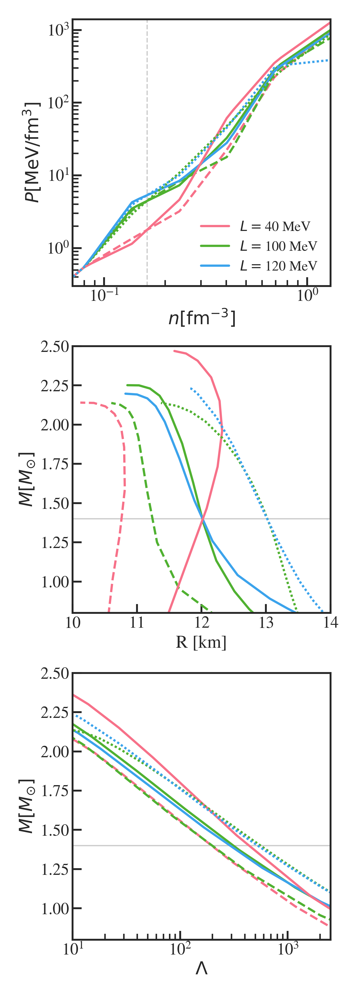
Figure 2: Equations of state included in our sample. The top panel shows the zero-temperature, $\beta$-equilibrium pressure; the middle panel shows the mass-radius relation; and the bottom panel shows the tidal deformabilities. The dashed lines indicate EoSs with $R_{1.4}\simeq 11$ km, which were constructed to have identical $\Lambda_{1.4}$=193. The solid lines correspond to EoSs with $R_{1.4}=12$ km, and the dotted lines correspond to the $R_{1.4}=13$ km EoSs.

II.1.1 Cold EoS in $\beta$-equilibrium

We model the zero-temperature, $\beta$-equilibrium EoS at densities above $0.5n_{\rm sat}$ with piecewise polytropes, as in Refs. Ozel and Psaltis (2009); Read et al. (2009); Steiner et al. (2010); Raithel et al. (2016). We use five polytropic segments, which are spaced uniformly in $\log{n}$ between 0.5 and 7.4 $n_{\rm sat}$. In order to ensure a smooth matching between the low- and high-density EoSs, we fix the polytopic pressure at $0.5n_{\rm sat}$ to that of SFHo. The pressures at the remaining fiducial densities serve as free parameters, which we vary to construct EoSs with particular values for the slope of the symmetry energy, the neutron star radius, and the neutron star tidal deformability. We require that the maximum mass of each EoS is at least $2M_{\odot}$, in order to satisfy observational constraints from massive pulsars Demorest et al. (2010); Antoniadis et al. (2013); Fonseca et al. (2016); Cromartie et al. (2019). Additionally, we require that each EoS remains causal, and we set a lower limit on the pressures at the first two fiducial densities ($P(0.86n_{\rm sat})>1.07$ MeV/fm³ and $P(1.5n_{\rm sat})>3.96$ MeV/fm³ ), which correspond to pressures obtained from the Argonne AV8 two-body potential Gandolfi et al. (2014). This provides a lower limit to the low-density pressure, under the assumption that the three-nucleon interaction is always repulsive. Because the expansion of nuclear interactions to few-body potentials breaks down at higher densities, we only impose these constraints on our first two fiducial densities. Additionally, for one EoS in our sample ($R_{1.4}=10.8$ km, $L=$40 MeV; see below), we relax the lower limit at $P(1.5n_{\rm sat})$ by 20%, in order to explore a broader region of parameter space. For additional details on the choice of these EoS constraints, see Ozel et al. (2016); Raithel et al. (2016).

Even though this parameterization is an agnostic way of describing the EoS, the polytropic pressure at $n_{\rm sat}$ still uniquely determines $L$, which we show as follows. We start with the general expression for the energy per baryon of zero-temperature nuclear matter,

$$E_{\rm nucl}(n,Y_{e},T=0)=E_{0}(n)+E_{\rm sym}(n)(1-2Y_{e})^{2}$$ (2)

where $n$ is the baryon number density, $Y_{e}$ is the electron fraction, and $E_{0}(n)$ is the energy of symmetric nuclear matter. The corresponding pressure is thus

$$P(n,Y_{e},T=0)=n^{2}\left[\frac{\partial E_{0}(n)}{\partial n}\right]+\\ n^{2}\left[\frac{\partial E_{\rm sym}(n)}{\partial n}\right](1-2Y_{e})^{2}.$$ (3)

In this derivation, we neglect the contribution of electrons, which add a $\lesssim 10$% correction into the determination of $L$ below. At the nuclear saturation density, $\partial E_{0}(n)/\partial n$ is zero by definition, and so the first term in eq. (3) vanishes. In order to simplify the second term, we use the fact that, for matter in $\beta$-equilibrium, the electron fraction is completely determined by the symmetry energy, i.e., $Y_{e,\beta}=Y_{e,\beta}(n,S,L)$, to leading-order in the symmetry energy expansion (see, e.g., Appendix A of Raithel et al., 2019). Following Raithel and Ozel (2019), we approximate the $\beta$-equilibrium neutron excess as

$$\left(1-2Y_{e,\beta}\right)^{2}=a+bu+\mathcal{O}(u^{2})$$ (4)

where $u\equiv(n/n_{\rm sat})-1$, $a=a(S)$, $b=b(S,L)$, and we have suppressed the dependencies of $Y_{e,\beta}$ on the density and symmetry energy parameters for clarity. With this approximation, we thus have $(1-2Y_{e,\beta})^{2}|_{n_{\rm sat}}\approx a$. Finally, we can further simplify eq. (3) by substituting in $L\equiv 3n_{\rm sat}\left(\partial E_{\rm sym}/\partial{n}\right)|_{n_{\rm sat}}$, which follows from the definition in eq. (1). Combining these results, the $\beta$-equilibrium pressure at $n_{\rm sat}$ is given by

$$P(n_{\rm sat},Y_{e,\beta},T=0)=\frac{an_{\rm sat}L}{3},$$ (5)

or

$$L=\frac{3P(n_{\rm sat},Y_{e,\beta},T=0)}{an_{\rm sat}}.$$ (6)

For a similar derivation, see Raithel and Ozel (2019). For the EoSs constructed in this paper, we fix $S$=32 MeV, in order to be consistent with recent theoretical and experimental constraints Li et al. (2021). Accordingly, $a(S)=0.833$ Raithel and Ozel (2019).

Using eq. (5), we vary the pressures in our piecewise polytropic model to fix $L$ to either 40, 100, or 120 MeV. These values were chosen in order to span the range of constraints from astrophysics and from the recent PREX-II measurement Li et al. (2021). Fixing $L$ effectively sets the pressures at the first two fiducial densities, which bracket $n_{\rm sat}$. We then vary the remaining pressures in the polytropic model to construct sets of EoSs that match in either $R_{1.4}$ or $\Lambda_{1.4}$. We show the resulting sample of seven EoSs in Fig. 2, along with the corresponding mass-radius and tidal deformability curves.

Approx. radius	$M_{\rm tot}[M_{\odot}]$	$q$	$L$ [MeV]	$R_{1.4}$ [km]	$R_{1.8}$ [km]	$\Lambda_{1.4}$	$\widetilde{\Lambda}$	$M_{\rm max}~{}[M_{\odot}]$
			40	10.8	10.8	193	237	2.14
R $\simeq$ 11	2.72	0.85	100	11.2	11.1	193	241	2.14
			40	12.0	12.3	425	517, 537	2.47
R = 12	2.72, 2.71	0.85, 1	100	12.0	11.9	311	394, 395	2.25
			120	12.0	11.6	287	364, 372	2.20
			100	13.0	12.5	557	699	2.14
R = 13	2.72	0.85	120	13.0	12.6	522	662	2.23

Table 1: Summary of equation of state (EoS) and binary configurations explored in this work.
Here, $M_{\rm tot}$ is the total gravitational mass at infinite separation of the binary, $q$ its mass ratio and $\tilde{\Lambda}$ its effective tidal deformability of the binary, defined as in eq. (5) of Favata (2014) . The EoS parameters are given by the slope, $L$, of the nuclear symmetry energy; the radii, $R_{1.4}$ and $R_{1.8}$, of a $1.4$ and $1.8,M_{\odot}$ neutron star (NS), respectively; the tidal deformability of $1.4\,M_{\odot}$ NS, $\Lambda_{1.4}$; and the maximum mass of a nonrotating NS, $M_{\rm max}$ .

Our final sample of EoSs contains three subsets which are designed for systematic comparison. In the first subset, we construct three EoSs that all predict $R_{1.4}=12$ km, but that span the full range of $L=40,$ 100, and 120 MeV. Because we span all three values of $L$ for this sample, these models will be the main focus of this paper. We additionally construct a set of two stiffer EoSs that predict a larger radius of $R_{1.4}=13$ km, for $L=100$ and 120 MeV. We find that it is not possible to construct a model with $R_{1.4}=13$ km and $L=40$ MeV without violating causality, within the particular polytropic framework used in this work. As a result, the $R_{1.4}=13$ km EoSs span just the larger values of $L=100$ and 120 MeV. Finally, we construct a set of softer EoSs, which were designed to match exactly in $\Lambda_{1.4}$, rather than in their radii. This allows us to study whether varying the tidal deformability, radius, or $L$ has a larger impact on the post-merger properties. For the softer set of EoSs, we focus on $L=40$ and 100 MeV, with $\Lambda_{1.4}=193$ for both cases, and $R_{1.4}=10.8$ and 11.2 km, respectively. The complete sample is shown in Fig. 2, and their characteristic properties are summarized in Table 1.

II.1.2 Extrapolation to finite temperatures and arbitrary electron fraction

The piecewise polytropic framework is used to characterize zero-temperature, $\beta$-equilibrium matter at densities above $0.5n_{\rm sat}$. However, in a neutron star merger, the post-merger temperatures can reach several tens of MeV and the electron fraction can also deviate from the initial $\beta$-equilibrium composition (e.g., Oechslin et al., 2007; Sekiguchi et al., 2011; Bernuzzi et al., 2016; Perego et al., 2019). In this section, we describe the key features of our extrapolation of the piecewise polytropes to finite temperatures and arbitrary electron fraction, which follows the framework of Ref. Raithel et al. (2019). For complete details on how the pressure and energy are calculated at fixed $n$, $T$, and $Y_{e}$, see Boxes I and II of that work.

We extrapolate to finite-temperatures using the $M^{*}$-model, which provides an approximation of the thermal pressure, including the leading-order effects of degeneracy at high densities Raithel et al. (2019). For all EoSs constructed in this paper, we use an identical set of $M^{*}$-parameters, $n_{0}$=0.12 fm^-3 and $\alpha=0.8$, which are consistent with the values inferred from a sample of nine of finite-temperature EoS tables Raithel et al. (2019).

The extrapolation from $\beta$-equilibrium to arbitrary $Y_{e}$ utilizes the leading order expansion coefficients of the symmetry energy, $S$ and $L$, as well as an additional parameter $\gamma$, which characterizes the density dependence of interactions between the particles. For all EOSs in our sample, we fix $S$=32 MeV, as described in Sec. II.1.1. The slope $L$ is set according to eq. (6), and we choose $\gamma=0.6$, which is consistent with the range of values inferred from tabulated EoSs Raithel et al. (2019).

We note that, for $n\lesssim 0.5n_{\rm sat}$, the nuclear symmetry energy framework breaks down, due to the formation of bound nuclei. This complicates the extrapolation from $\beta$-equilibrium to arbitrary $Y_{e}$, which is grounded in the symmetry energy formalism. In order to avoid these issues, we switch to the tabulated EoS SFHo at densities below $0.5n_{\rm sat}$. The matching of this low-density EoS to our high-density, finite-temperature models is performed following Schneider et al. (2017), with a transition window from $n=6.3\times 10^{-5}$ to 0.08 fm^-3 (see also Ref. Most et al. (2019a))). Additionally, across this transition window, we switch from the complete model for $E_{\rm sym}(n)$ to a decaying power-law function, with parameters that are chosen to ensure that the extrapolation to arbitrary $Y_{e}$ remains realistic across the window. For additional details, see Appendix A.

The nuclear symmetry energy expansion formalism is also expected to break down at very high densities of a few times $n_{\rm sat}$, where additional degrees of freedom may become important. We do not account for non-nucleonic degrees of freedom in this paper, and leave the exploration of such effects to future work.

Finally, we note that in addition to the pressure, energy, and sound speed (which are all calculated following Ref. Raithel et al. (2019)), the numerical evolution also requires input for the chemical potentials, which are used to model the neutrino transport (see Sec. II.2). We describe the calculation of the chemical potentials in Appendix B.

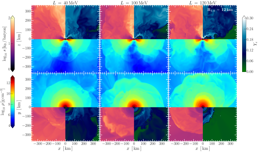
Figure 3: Two-dimensional spatial distributions of the rest-mass density $\rho$, temperature $T$, electron fraction $Y_{e}$, and entropy $s$ per baryon. Shown are meridional (top) and equatorial (bottom) views for three different values of the slope $L$ of the nuclear symmetry energy. The results shown are for the $R_{1.4}\,=\,12\,\rm km$ models with mass ratio $q=0.85$ at time $t=25\,\rm ms$ after merger.

II.2 Numerical Setup

In this work, we simulate the final orbits, merger, and post-merger phase of a binary neutron star coalescence. This requires us to model both the evolution of the fluid as well as the self-consistently coupled dynamical evolution of the space-time. For the latter, we solve the equations of general relativity using the Z4c Hilditch et al. (2013); Bernuzzi and Hilditch (2010) formulation, which is based on the Z4 formulation Bona et al. (2003), that allows for a dynamical damping of constraint violations to the Einstein field equations Gundlach et al. (2005). Following Weyhausen et al. (2012), we choose damping parameters $\kappa_{1}=0.02$ and $\kappa_{2}=0$. The gauge conditions adopt moving puncture gauges, i.e. 1+log slicing with Gamma-driver conditions (Alcubierre et al., 2003), with damping parameter $\eta=0.5$. We further find it beneficial to add an inverse radial fall-off to the damping parameters outside of a sphere of $r=500\,\rm km$, to preserve numerical stability Schnetter (2010). To damp high-frequency noise in the gravitational field sector, we add Kreiss-Oliger dissipation Babiuc et al. (2008).

On the dynamically evolved background, we solve the equations of ideal general-relativistic (magneto-)hydrodynamics (GRMHD) Duez et al. (2005); Shibata and Sekiguchi (2005), in the limit of vanishing magnetic field strength. Weak interactions are included following the leakage prescription outlined in Ruffert et al. (1996a); Rosswog and Liebendoerfer (2003), which accounts for local energy losses and composition changes due to neutrino interactions.

We solve these equations using the Frankfurt-/IllinoisGRMHD code (FIL) Most et al. (2019b, a), which is derived from the publicly available IllinoisGRMHD code ( ILGRMHD ) Etienne et al. (2015). To solve the Einstein equations, FIL provides a fourth-order accurate numerical implementation of the Z4c system using the methods outlined in Zlochower et al. (2005).
Different from ILGRMHD, FIL utilizes a fourth-order accurate conservative finite-difference algorithm based on the ECHO scheme to solve the GRMHD equations Del Zanna et al. (2007). Crucially for this work, FIL provides its own microphysics infrastructure, which can handle fully tabulated EoSs. The codes makes use of the publicly available Einstein Toolkit infrastructure (Loffler et al., 2012) and specifically the Carpet moving boxes refinement code Schnetter et al. (2004). Specifically, we set up our simulation domain to extend to an outer boundary of $3022\,\rm km$ in each direction and to consist of 8 refinement levels of doubling resolution, where the finest one covering the stars has a resolution of $262\,\rm m$. For computational efficiency, we employ reflection symmetry across the vertical $z$-direction.

II.3 Initial conditions

We model the initial irrotational neutron star binaries in quasi-circular equilibrium Gourgoulhon et al. (2001) using the LORENE code. The two neutron stars are placed at an initial separation of $45\,\rm km$ and are constructed for each of the EoSs outlined in Sec. II.1. The binary parameters are modelled after the GW170817 event Abbott et al. (2017b); Abbott et al. (2019b). In particular we adopt two mass ratios $q=\left[0.85;1.0\right]$, where the latter is only used with $R_{1.4}=12\,\rm km$ EoSs. This fixes the total mass $M$ of the system, via the chirp mass $\mathcal{M}=Mq^{3/5}/\left(1+q\right)^{6/5}=1.186\,M_{\odot}$ (Abbott et al., 2019b).

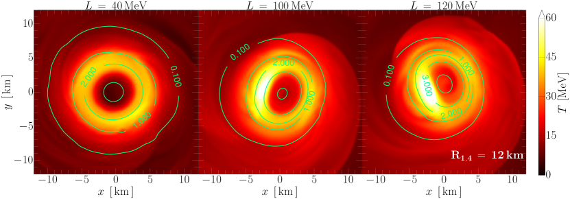
Figure 4: Temperature $T$ in the equatorial plane at $t\simeq$ $20\,\rm ms$ after merger for unequal mass $(q=0.85)$ mergers with EoSs having a characteristic radius of $R_{1.4}\,=\,12\rm km$. The green lines indicate contours of constant rest-mass density, with values labelled with respect to the nuclear saturation density. The different panels show results for varying slope parameter $L$ from 40 to 120 MeV.

III Results

We now turn to the results of our simulations, with an emphasis on the unequal mass case $(q=0.85)$, which most closely matches the masses inferred from GW170817. Starting from a description of the general dynamics and remnant properties, we will present a discussion of the mass ejecta and of the gravitational wave signals expected for various choices of the slope of the symmetry energy $L$.

Since the main goal of this paper is to determine how $L$ affects the early post-merger phase, we focus our attention on the dynamics in the first few tens of milliseconds after merger. During this time, high temperatures will be reached during merger Oechslin et al. (2007); Sekiguchi et al. (2011); Bernuzzi et al. (2016); Perego et al. (2019), post-merger bounces can drive an early mass ejection Nedora et al. (2020), and the rotating remnant will emit significant GWs. At the end of this process, the former two neutron star cores will have fused into a single core, with continued, diminishing gravitational wave emission leading to an axisymmetrization of the remnant. This newly formed massive neutron star will be hot and rapidly, differentially rotating Hanauske et al. (2017), unless strong shear viscosity is present Radice (2017); Shibata and Kiuchi (2017). This remnant will set the stage for long-term mass ejection and neutrino emission.

For all EoSs considered in this paper except one, we find that the remnants survive until the end of our simulations ($t\simeq 25$ ms post-merger). The sole exception is the EoS with $L\,=\,40\,\rm MeV$ and $R_{1.4}\,=\,10.8\,\rm km$, which collapses after $15\,\rm ms$. When comparing to this EoS, we will accordingly limit our comparisons to the first $15\,\rm ms$ post-merger. For all other EoSs, we will present results from the end of our simulations (about $25\,\rm ms$ post merger), unless otherwise specified.

In order to provide a first indication of how the post-merger remnant and early mass ejection depend on the slope of the symmetry energy, Fig. 3 shows equatorial and meridional cuts of the rest-mass density, $\rho$, specific entropy, $s$, and electron fraction, $Y_{e}$, about $25\,\rm ms$ after merger. To aid the comparison, we focus here on models with radii $R_{1.4}\,=\,12\,\rm km$. Starting out with the rest-mass density, in the equatorial plane (bottom row of Fig. 3 ) we can see clear differences in the total amount of mass ejection. The $L\,=\,120\,\rm MeV$ case shows extended shock fronts with densities $\rho<10^{10}\,\rm g\,cm^{-3}$, that are reduced in size for the $L\,=\,40\,\rm MeV$ case. Additionally, the $L\,=\,40\,\rm MeV$ profiles are much more axisymmetric than for higher values of $L$.

Looking at the electron fractions $Y_{e}$, we find that the disk and most of the ejecta are very neutron rich, i.e. $Y_{e}<0.02$ (green regions) for the large $L$ EoSs, whereas the proton fraction is slightly enhanced, $Y_{e}\simeq 0.1$, for low $L$. The electron fractions in the polar region are overall comparable between the EoSs, but are slightly more proton rich in the $L\,=\,40\,\rm MeV$, which is related to much higher shock heating, as evidenced by the enhanced specific entropies $s$ for this EoS. Specifically, we also find differences in the specific entropies reached for each of our EoSs, as shown in the pink panels of Fig. 3. We find that the merger with $L\,=\,100\rm MeV$ reaches the highest specific entropy, in both the equatorial plane and along the polar axis. However, for all values of $L$, we find that $s$ can exceed 10 $\rm{k_{B}/baryon}$, in the low-density outflows. Since $s$ is a proxy for the amount of shock heating taking place, we are led to conclude that shock heating will be important for all values of $L$, for the $R_{1.4}\,=\,12\rm km$ models in our sample. We discuss these properties of the ejecta in further detail below.

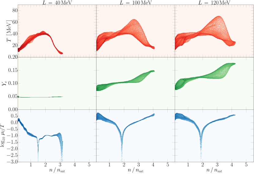
Figure 5: Temperatures $T$, electron fractions $Y_{e}$ and lepton chemical potential $\mu_{l}$ probed at different densities $n$ in the massive neutron star remnant. The densities are stated relative to saturation density $n_{\rm sat}$. The models are the same as shown in Fig. 4.

III.1 Remnant properties

We now turn to the general properties of the hypermassive neutron star remnant, and how it is impacted by differences in the slope $L$ of the nuclear symmetry energy. Since we have three different slope values available for the $R_{1.4}\,=\,12\rm km$ case (see Sec. II.1), we will mainly focus on these models in this section.

We begin by discussing the overall structure and thermodynamic conditions present in the hypermassive neutron star. Figure 4 shows the temperature and density distribution in the equatorial plane, at $\simeq 20\,\rm ms$ after merger. We can see that there are several differences between the models. Starting for the $L\,=\,40\,\rm MeV$ model (left panel), we see that after merger temperatures of about $40\,\rm MeV$ are reached in a hot ring with densities between $1-2\,n_{\rm sat}$. Surprisingly, despite starting from an initially asymmetric merger, the system has quickly circularized. This behavior will be more closely examined in Sec. III.3 in the context of the associated gravitational wave emission and the decay of the $m=1$ component. For the $L=\,100$ and $120\,\rm MeV$ cases, we instead find that the hot ring is highly asymmetric, with temperatures $>60\,\rm MeV$ being reached in parts of the hot ring. Similar to what has been found by varying the finite-temperature part of the EoS Raithel et al. (2021), we find that changes in $L$ lead to different temperatures in the colder center of the star. This suggests that, at least within some part of the parameter space, finite temperature effects might be degenerate with changes to the cold EoS, in determining the thermal profile of the remnant. Such temperature differences might be crucial when determining the microphysical conditions necessary for (bulk-) viscous effects to become important Most et al. (2021), and may also influence the local neutrino emissivity of the remnant and, as a result, the cooling and eventual neutrino irradiation of the disk.

Overall, we find that the maximum temperatures reached in the merger correlate strongly with the initial neutron star radius, as summarized in Table 2. Mergers with $R_{1.4}\,=\,11\,\rm km$ reach temperatures above $120\,\rm MeV$ at merger, whereas those with $R_{1.4}\,=\,13\,\rm km$ only reach temperatures $\lesssim 100\,\rm MeV$. This is consistent with previous findings that more compact neutron stars collide with higher impact velocities Bauswein et al. (2013), and thus would be expected to experience stronger shock heating. At late times within the massive neutron star remnant, however, the temperatures are less strongly correlated with $R_{1.4}$, as can be seen in Fig. 4, where for all EoSs with $R_{1.4}=12$ km, the maximum temperatures vary between $40\lesssim T^{\rm max}_{\rm final}\lesssim 70$ MeV. Instead, we find that the maximum temperature of the late-time remnant correlates weakly with the radii at high masses, i.e. for $M\,\geq\,1.8\,M_{\odot}$. That is, EoSs with small $R_{1.8}$ overall reach temperatures above $60\,\rm MeV$, whereas EoSs with larger ($R_{1.8}>12\,\rm km$), only reach temperatures $<50\,\rm MeV$. Therefore, it seems likely that the late-time remnant temperatures are, at least in part, governed by the high density part of the cold EoS. We list the values of $R_{1.8}$ in Table 1 for reference, while the maximum merger and late-time temperatures are summarized in Table 2.

We continue our description of the remnant temperature by studying the distribution of temperatures in terms of the densities at which they occur, again focusing on the $R_{1.4}=12$ km models. Previous studies have considered these conditions either in the general thermodynamics of the merger Perego et al. (2019); Hanauske et al. (2019) or the appearance of a hot quark-matter phase Most et al. (2020); Prakash et al. (2021). In the top row of Fig. 5, we now directly compare the thermodynamic conditions present at a given density. We can see that due to differences in the cold EoS, and hence in $L$, different densities are reached. In particular, the $L=40\,\rm MeV$ merger probes lower densities of around $3\,\rm n_{\rm sat}$, while higher values of $L$ lead to densities beyond $4\,\rm n_{\rm sat}$ being probed in the post merger. This is a direct result of the overall stiffness of these EoSs. Most strikingly, in the case of the $L\,=\,40\,\rm MeV$ EoS, the temperature distribution is very narrow, and follows an almost univariate profile with the density. On the other hand, the temperatures probed in the $L\,\geq\,100\,\rm MeV$ cases are more broadly distributed, with temperatures of up to $70\,\rm MeV$ being reached. Also in these cases, a simple mapping between $n$ and $T$ is no longer possible, as the range in temperatures can be quite broad for a given density, e.g. $30\,\rm MeV$ differences for matter at $n\simeq 3\,n_{\rm sat}$.

At the same time, we can also compare how the electron fraction of the system varies, which would be a proxy for out-of-weak-equilibrium effects. While initially the electron fraction in the inspiral will be fixed at cold $\beta$-equilibrium, at high temperatures the conditions for $\beta$-equilibrium are modified. Indeed, we can see that for the coldest case, which corresponds to $L\,=\,40\,\rm MeV$, the electron fraction is almost constant with a very narrow distribution, with $Y_{e}\simeq 0.05$. For higher values of $L$, $Y_{e}$ increases to higher densities, as expected from cold $\beta$-equilibrium, and also attains a considerable spread, as a result of the large spread in $T$ for these EoSs. Nevertheless, even for the highest values of $L$ considered here, the electron fraction remains low, $Y_{e}<0.2$.

To reinforce these observations, Fig. 4 also shows the lepton chemical potential $\mu_{l}$, which vanishes in $\beta$-equilibrium. From this, we can see that indeed out-of-equilibrium effects are likely small for the $L\,=\,40\,\rm MeV$ case, but may be significant for matter above $2\,n_{\rm sat}$ for larger L. This could have implications on the long-term thermal evolution and neutrino cooling of the remnant Fujibayashi et al. (2017, 2018).

III.2 Mass ejection

In this section we focus on the mass dynamically ejected during the merger process, see e.g. Sekiguchi et al. (2016); Lehner et al. (2016a); Bovard et al. (2017); Radice et al. (2018). Although this is in most cases only a small contribution to the overall amount of ejecta from the system Abbott et al. (2017c), the exact details typically depend on the EoS and the mass ratios used in the simulation Sekiguchi et al. (2016). Additionally, the recent observation of an X-ray rebrightening Hajela et al. (2021); Balasubramanian et al. (2021), potentially associated with the presence of relativistic fast ejecta Hotokezaka et al. (2018); Nedora et al. (2021), has resulted in a recent interest into the properties of dynamical mass ejection.

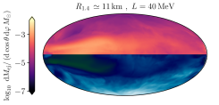
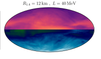
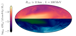
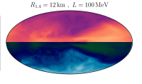
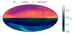
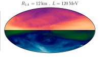
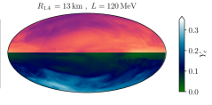
Figure 6: Time-integrated ejected mass $M_{\rm ej}$ and mass-weighted average electron fraction $Y_{e}$ projected onto a sphere at radius $r=295\,\rm km$ from the origin. The data is shown using Mollweide projection for the unequal mass models.

In this work, we extract the amount of mass ejecta on a spherical detector placed at a radial coordinate $r=295\,\rm km$ from the merger site. We record the mass flux

$$\dot{M}_{\rm ej}=\oint_{r\,=\,295\,\rm km}\sqrt{\gamma}\rho u^{i}\,{\rm d}S_{i}\,,$$ (7)

temperature $T$ and electron fraction $Y_{e}$ of the ejecta as the pass through the surface $S$. Here $\rho$ is the rest-mass density, $u^{i}$ the spatial component of the fluid four-velocity, and $\gamma$ is the determinant of the 3-metric. In order to determine whether a fluid element crossing the detector is unbound, we use the $u_{t}<-1$ criterion Bovard and Rezzolla (2017). We point out that this will slightly underestimate the amount of unbound ejecta, as it neglects the contribution of the internal energy.

We then time integrate the the mass flux to compute the amount of mass ejection ${\rm d}M_{\rm ej}/{\rm d}\Omega$ per solid angle. Additionally, we also compute the mass-weighted electron fraction as an indicator for average nuclear composition.

The resulting spatial and compositional distributions of the ejecta for the unequal mass mergers ($q=0.85$) are shown in Fig. 6 using Mollweide projection. Starting with the reference case of $R_{1.4}\,=\,12\,\rm km$, we observe the following differences between the small $L\,=\,40\,\rm MeV$ case and the $L\,>\,100\,\rm MeV$ cases. First, the $L\,=\,40\,\rm MeV$ case features a rather spatially isotropic distribution of mass ejecta. Additionally, the electron fraction reaches the highest average values in all three values of $L$, having $Y_{e}>0.25$ for large parts of the mass ejection, for the $R_{1.4}\,=\,12\,\rm km$ EoSs. With increasing slope parameter $L$, we find that the ejection becomes more equatorial, with the largest amounts of ejecta in the $L\,=\,120\,\rm MeV$ case. Consistent with the increase of equatorial ejection, which is likely tidally driven Sekiguchi et al. (2015), the electron fraction of the ejecta decreases to values below $Y_{e}<0.1$ in those regions. Overall the electron fraction reaches lower values also in polar regions for large $L$, compared to the $L\,=\,40\,\rm MeV$ cases. For unequal mass mergers, these trends are inversely correlated with $\Lambda_{1.4}$, whereas for equal masses the trend is less clear. From Fig. 2, we can see that there are strong variations in radius of the secondary star ($M_{2}=1.25\,M_{\odot}$ for the unequal mass binary). As a result, we find that for those systems, tidal effects take over that correlate more strongly with the compactness. For those mass ratios, the larger $L$ models tend to produce more equatorial ejetca, despite having smaller tidal deformabilities. Albeit somewhat counter intuitive, there have been previous examples in the literature in which tidal disruption was better captured in terms of the compactness, than with the tidal deformability Foucart et al. (2018). These results suggest that perhaps the picture is more complicated than either a single compactness or $\Lambda$ parameter can generically capture. Qualitatively, the same behaviour also applies to the $R_{1.4}\,\simeq\,11\,\rm km$ cases (Fig. 6, left column), where the $L\,=\,100\,\rm MeV$ simulation features enhanced neutron rich outflows in the equatorial plane compared with the $L\,=\,40\,\rm MeV$ case, despite the fact that these EoSs have an identical $\Lambda_{1.4}$. Finally, as we saw for the $R\,=\,12\,\rm km$ models, the ejection in the $R_{1.4}\,=\,13\,\rm km$ cases is very similar for $L$=100 MeV compared to 120 MeV.

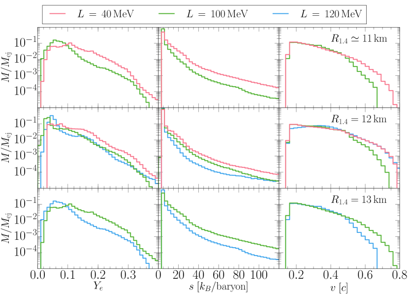
Figure 7: Histograms of the electron fraction, the average entropy per baryon, and the velocity of the dynamical mass ejecta for simulations with mass ratios $q=0.85$. The histograms refer to time integrated quantities and have been normalized to the respective amount of total mass ejection $M_{\rm ej}$. The different colours refer to simulations with different slopes $L$ of the nuclear symmetry energy, while $R_{1.4}$ denotes the radius a $1.4\,M_{\odot}$ star for each EoS.

In order to provide a more quantitative description of the mass ejection, we next consider one-dimensional histograms of the entropy per baryon, $s$ , electron fraction, $Y_{e}$, and velocity, $v$, for the dynamical ejecta. These are shown in Fig. 7. Starting with the average electron fraction we can see the overall distributions for the $R_{1.4}\,=\,12\,\rm km$ EoSs are surprisingly similar. As discussed for Fig. 6, there are differences for the lowest $Y_{e}$ bins, with large $L$ models containing slightly more mass at small $Y_{e}<0.05$, but the fall-off at large $Y_{e}$ is nearly identical for all values of $L$. This behaviour is very similar for the $R_{1.4}\,\simeq\,11\,\rm km$ cases. Interestingly, the difference between the $L\,=\,100\,\rm MeV$ and $L\,=\,120\,\rm MeV$ at intermediate electron fractions $Y_{e}>0.15$ is more pronounced for large stars with $R_{1.4}\,\simeq\,13\,\rm km$; however, these differences remain small.

Different from essentially all previous studies (see e.g. Refs. Baiotti and Rezzolla (2017); Dietrich et al. (2021); Radice et al. (2020) for a review), our EoS are specifically constructed to vary only in the high-density part, while also using the same finite-temperature model (see Sec. II.1). In all cases, the low density EoS is, however, the same. Given the large insensitivity of the results to changes in high-density physics between the models, this leads us to conjecture that the composition of the ejecta is largely determined by low density EoS, which governs the outer regions of the stars from which they are ejected.

In contrast, when considering the distribution of entropies $s$ per baryon for the mass ejecta, we find a small trend with $L$. Specifically, we find that in all cases an ordering is present, where larger $L$ slope parameters can lead to a suppression of highly shocked material with large, $s\,>\,40\,\rm k_{B}\,/\,baryon$.

Finally, we comment on the prospect for high velocity ejecta, which is especially relevant in the context of the recently observed X-ray rebrightening of GW170817 Hotokezaka et al. (2018). We find that, in all cases, high velocity tails with $v>0.6\,c$ are present, which constitute about $1\%$ of the overall mass ejecta. Different from the specific entropy $s$, no concrete ordering in terms of $L$ can be inferred from our data. For large stars (bottom row of Fig. 7), higher values of $L$ lead to a suppression of fast ejecta. On the other hand, for $R_{1.4}\,=\,12\,\rm km$ models, large and small values of $L$ produce almost identical distributions, except at very low velocities. It, therefore, seems that the dependence of fast ejecta on nuclear parameters is more complicated, as already anticipated in earlier works Metzger et al. (2015); Hajela et al. (2021); Nedora et al. (2021).

$R_{1.4}$ [km]	$q$	$L$ [MeV]	$M^{\rm dyn}_{\rm ej}\,\left[10^{-3}\,M_{\odot}\right]$	$\left<v\right>\left[c\right]$	$\left<Y_{e}\right>$	$T^{\rm max}_{\rm mer}\left[\rm MeV\right]$	$T^{\rm max}_{\rm final}\left[\rm MeV\right]$
		40	2.2	0.34	0.10	136	63
$R_{1.4}$ $\simeq$ 11	0.85	100	5.3	0.36	0.07	120	66
		40	0.6	0.30	0.12	89	40
	0.85	100	2.5	0.30	0.08	95	60
		120	6.2	0.31	0.07	85	68
$R_{1.4}$ = 12
		40	1.2	0.28	0.09	97	46
	1.0	100	0.7	0.27	0.13	106	61
		120	0.8	0.31	0.13	129	52
		100	1.9	0.28	0.09	94	50
$R_{1.4}$ = 13	0.85	120	2.1	0.28	0.08	85	46

Table 2: Summary of remnant temperatures and the mass-averaged dynamical ejecta properties. $M_{\rm ej}^{\rm dyn}$ is the total amount of dynamical ejecta, while $\left<v\right>$ and $\left<Y_{e}\right>$ are the mass-averaged velocity and electron fraction of the dynamical ejecta, respectively. $T^{\rm max}_{\rm mer}$ is the maximum temperature achieved at densities above $n_{\rm sat}$ at the time of merger and $T^{\rm max}_{\rm final}$ is the maximum temperature in the remnant ($n>n_{\rm sat}$) at the end of our simulations.

III.3 Gravitational waves

Finally, we consider the gravitational wave (GW) emission from the various EoSs in our sample. While several previous studies have used the inspiral of GW170817 to constrain $L$ (e.g., Zhang and Li, 2019; Raithel and Ozel, 2019; Tsang et al., 2019; Essick et al., 2021), the dependence of the post-merger GW signal on $L$ has never before been systematically explored. Consistent with the rest of this paper, we thus focus our analysis in this section on the post-merger GW emission. Details on the analysis methods are summarized in Appendix C.

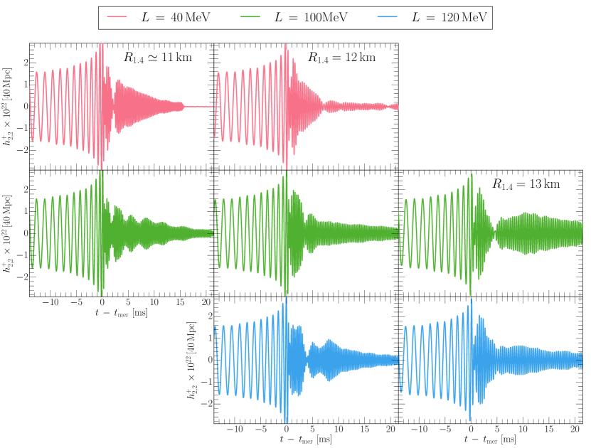
Figure 8: Gravitational wave strain for the $q=0.85$ binaries, viewed face-on at 40 Mpc. The different radii are plotted in each column, while the rows show different values of $L$. All waveforms are aligned at the time of merger. We find significant differences in the post-merger GW signals, even for EoSs with the same $R_{1.4}$.

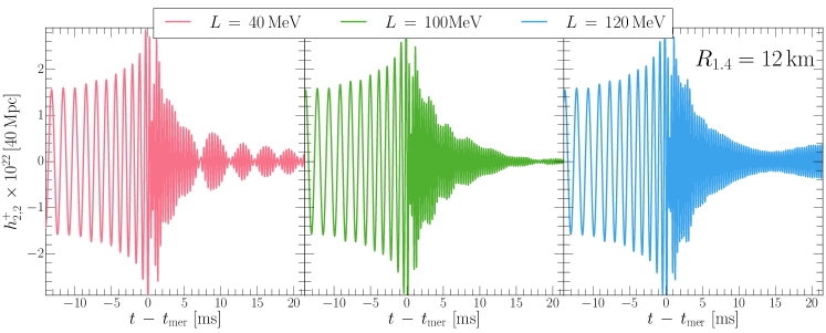
Figure 9: Same as Fig. 8, but for the equal-mass binaries.

III.3.1 Gravitational wave signals

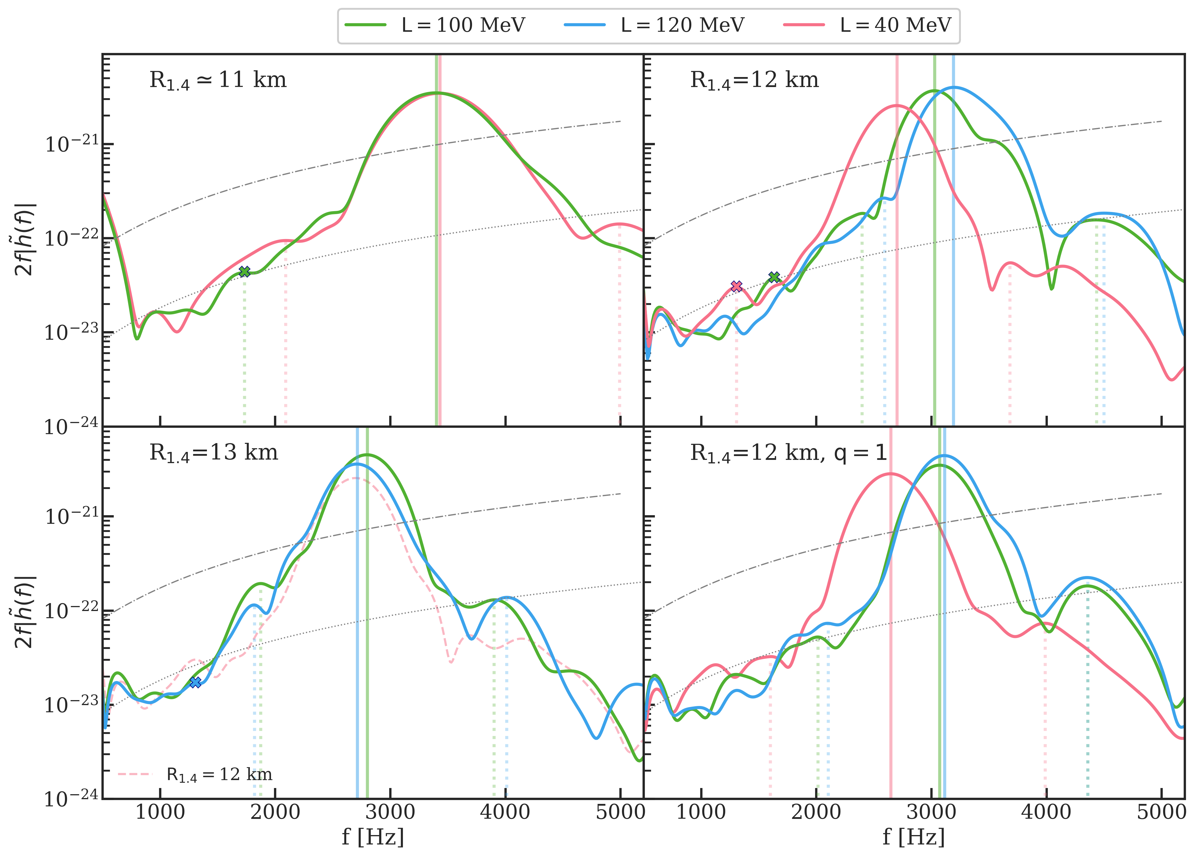
Figure 10: Characteristic strain, including all $\ell$=2, 3 modes, for a face-on merger at 40 Mpc. The top two and bottom left panels are for the $q=0.85$ binaries, while the bottom right panel corresponds to the equal-mass binary. The vertical solid line marks the dominant $f_{2}$ spectral peak, while the dotted lines indicate the location of the secondary peaks $f_{1}$ and $f_{3}$. The markers indicate the approximate location of spectral peaks associated with the $m=1$ mode, which are expected to occur at $\simeq f_{2}/2$ where present. Finally, the $R_{1.4}=12$ km, $L=40$ MeV EoS is also plotted in the lower left panel with the faded, dashed pink line, to illustrate the similarity of this spectrum with the $R_{1.4}=13$ km spectra. The gray dash-dot and dotted lines indicate the design sensitivity curves for advanced LIGO Aasi et al. (2015) and Einstein Telescope Punturo et al. (2010), respectively.

We start by showing the $\ell=m=2$ component of the plus-polarized GW strains, $h_{2,2}^{+}$, for the $q=0.85$ binaries in Fig. 8. These signals correspond to a face-on merger located at 40 Mpc. In all panels, we have aligned the signals at the time of merger, $t_{\rm mer}$, which we define as the time at which $\left|h_{+}^{2,2}\right|$ reaches a maximum. Although the EoSs are constructed with fixed radii $R_{1.4}$, their tidal deformabilities can differ significantly, see Table 1. This leads to considerable phase difference of the waveforms by the time of merger. Only the EoSs with $R_{1.4}\simeq 11$ km have equal values of $\Lambda_{1.4}$, and these resulting binaries indeed have identical inspirals.

From Fig. 8, we observe significant differences in both the amplitude and beat frequencies of the decaying post-merger GWs for the various EoSs in our sample. We find differences between EoSs both with common $R_{1.4}=12$ or 13 km, and also between EoSs with identical tidal deformabilities (corresponding to the $R_{1.4}\simeq 11$ km models, shown in the first column of Fig. 8). This suggests already that the values of $R_{1.4}$ or $\Lambda_{1.4}$ do not uniquely govern the post-merger GW emission. We also find differences in the post-merger GWs from the equal-mass binaries with $R_{1.4}$=12 km, which are shown in Fig. 9.

We explore the spectral content of these post-merger GWs in more detail by calculating their characteristic strain via eq. (22), which we show in Fig. 10, again for a face-on merger located at $40$ Mpc. The spectra in Fig. 10 show several well-defined peaks, which we highlight with vertical lines. The dominant peak, which is marked with a solid vertical line and which we call $f_{2}$, is located in each spectra at $\sim\,2800-3200$ Hz. We also find secondary peaks located to either side of $f_{2}$, which we call $f_{1}$ and $f_{3}$ and which we mark with dotted vertical lines. Finally, in a subset of the EoSs, we find a possible peak located at $\sim f_{2}/2$, which we call $f_{m=1}$ and we mark with a cross. We summarize the location of all peaks in Table 3.

We note that the $f_{2}$ spectral peak is typically associated with quadrupolar oscillations of the remnant, while the origin of the secondary peaks remains under debate Stergioulas et al. (2011); Takami et al. (2014); Baiotti and Rezzolla (2017); Paschalidis and Stergioulas (2017); Bauswein and Stergioulas (2019). We do not distinguish between the proposed origins in the present work, but rather treat the secondary peaks agnostically, reporting simply the relative alignment of the peaks for each EoS. Additionally, we note that for some EoSs in our sample, these secondary peaks are only weakly resolved, and their exact alignment should be interpreted with a grain of salt. In the following, we, therefore, focus in particular on the dominant peak, $f_{2}$, and we return to a discussion of $f_{m=1}$ in Sec. III.3.4.

In order to further quantify the differences of the gravitational waveforms in the post-merger phase, we compute detector-dependent overlap integrals, ${O}$, assuming the design sensitivity of Advanced LIGO Aasi et al. (2015) and a face-on source located at 40 Mpc (see Appendix C for details). The overlap integral is defined such that $O\lesssim 0.992$ is required to marginally distinguish two waveforms with SNR of 8 Lindblom et al. (2008); McWilliams et al. (2010). For the $R_{1.4}\simeq 11$ km EoSs, we find that the post-merger GW signals are indistinguishable ($O=0.999$). The top left panel of Fig. 10 shows that location of the dominant spectral peaks are nearly identical as well (to within $\lesssim$30 Hz). These two EoSs have similar $R_{1.4}$ and identical $\Lambda_{1.4}=193$, yet differ substantially in $L$, ranging from 40 to 100 MeV. We plan to further explore this similarity of the GW emission for these two EoSs in a follow-up paper. We note, for now, that the similarity of these spectra suggests that $L$ does not have a clear imprint on the post-merger GW signal for this EoS.

The weak dependence of the post-merger GW signal on $L$ extends to larger values of $L$ as well. From the $R_{1.4}$=13 km EoSs, which have larger, albeit more similar, values of $L=100$ and 120 MeV, we find that the post-merger GWs are only marginally distinguishable ($O=0.97$) with Advanced LIGO at design sensitivity. Additionally, the maximum difference in $f_{1}$, $f_{2}$, and $f_{3}$ for these EoSs is $\lesssim 90$ Hz, suggesting again only a weak imprint of $L$ on the post-merger signal.

In contrast, for the $R_{1.4}$=12 km EoSs, we find a large difference between the GW signals for the $L=40$ MeV EoS compared to the EoSs with either $L=100$ or 120 MeV. These differences hold for both the equal and unequal-mass binaries. For the case of the unequal mass binary, the overlap integral between the $L=40$ and 100 (120) MeV EoSs is 0.57 (0.34), while we additionally find differences of up to 490 Hz in the location of $f_{2}$ between these EoSs. The waveforms for these EoSs are thus clearly distinguishable for Advanced LIGO at design sensitivity. For the $R_{1.4}=12$ km EoSs with $L=100$ and 120 MeV, the overlap integral is still 0.88, indicating that even these signals can be distinguished with the sensitivity of Advanced LIGO. We find similar results for the equal mass binary, although for this case, the $L=100$ and 120 MeV spectra are only marginally distinguishable ($O=0.992$; see also Fig. 9).

$R_{1.4}$ [km]	$q$	$L$ [MeV]	$f_{1}$ [kHz]	$f_{2}$ [kHz]	$f_{3}$ [kHz]
		40	2.09	3.43	4.99
$R_{1.4}$ $\simeq$ 11	0.85	100	1.73	3.40	7.29
		40	1.31	2.70	3.68
	0.85	100	2.40	3.03	4.43
		120	2.59	3.19	4.50
$R_{1.4}$ = 12
		40	1.60	2.65	3.99
	1.0	100	2.02	3.07	4.36
		120	2.10	3.12	4.36
		100	1.87	2.80	3.90
$R_{1.4}$ = 13	0.85	120	1.82	2.71	4.01

Table 3: Summary of post-merger GW frequencies. See the description in the text for further details.

III.3.2 Correlation of $f_{2}$ with the high-density EoS

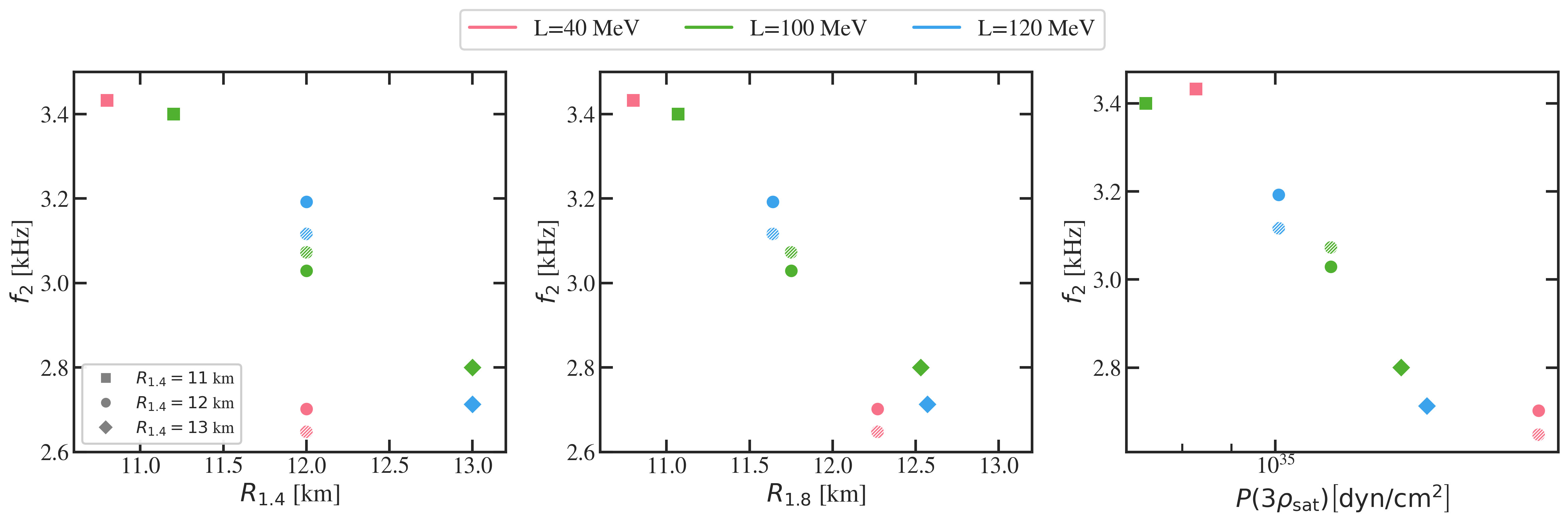
Figure 11: Correlations between the peak frequency $f_{2}$ and the radii $R_{1.4}$ and $R_{1.8}$ of $1.4\,M_{\odot}$ and $1.8\,M_{\odot}$ neutron stars, respectively. We also show correlations with the pressure $P$ at density $n=3\,n_{\rm sat}$. The different colors correspond to the value of $L$, while the different symbol shapes indicate $R_{1.4}$ for our chosen EoSs. The hatched symbols correspond to the results from the equal-mass binaries, while the solid-fill symbols correspond to the $q=0.85$ binaries. We find a significant scatter in the correlation between $f_{2}$ and $R_{1.4}$, and that $f_{2}$ instead correlates more closely with the high-density part of the EoS, parameterized here either with $R_{1.8}$ or $P_{3n_{\rm sat}}$.

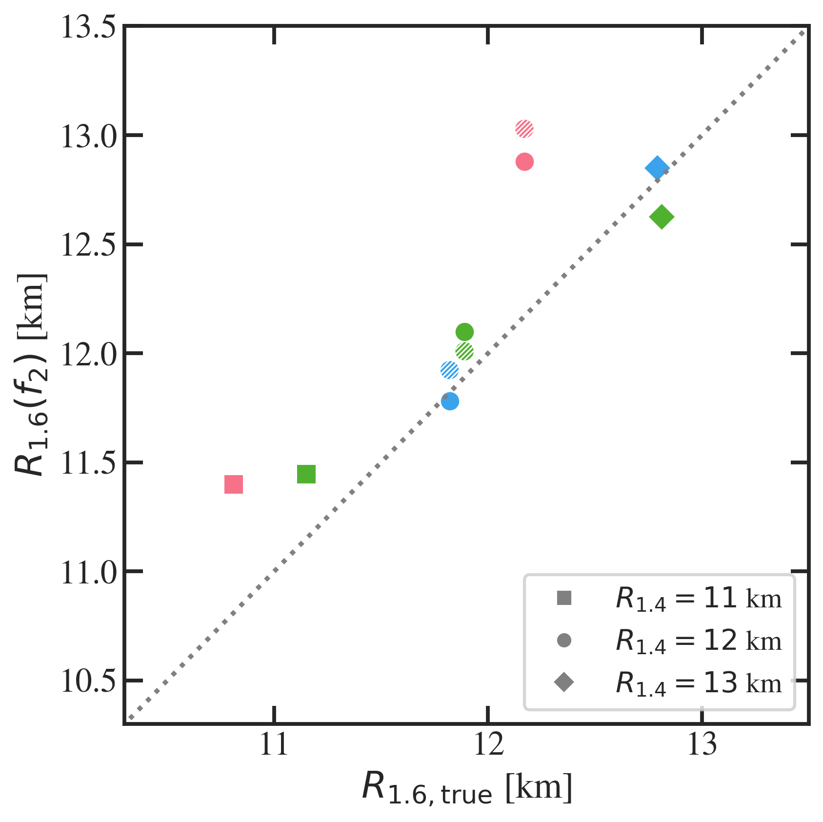
Figure 12: Inferred radius as a function of the true (inputted) radius, for each of the binaries in this work. The color scheme and symbols are as in Fig. 11. We calculate $R_{1.6}(f_{2})$ using the universal relationship from eq. (21) of Vretinaris et al. (2020). We find that using this standard fitting formula with these more extremal EoSs leads to inferred errors of up to 0.86 km in the radius for the EoSs included in this work.

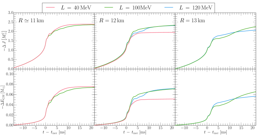
Figure 13: Gravitational wave energy ($\Delta E_{\rm GW}$) and angular momentum losses $\Delta J$ for the unequal mass mergers $q=0.85$. Different colors correspond to different slope parameters $L$.

We therefore find that, although varying $L$ leads to significantly different GW emission for the EoSs with $R_{1.4}=12$ km, there is no clear trend between $L$ and the post-merger GWs that persists for all EoSs in our sample. Instead, we find that $f_{2}$ correlates more strongly with the high-density EoS, as we show in Fig. 11. The three panels of Fig. 11 shows $f_{2}$ as a function of $R_{1.4}$, $R_{1.8}$, and the pressure at $3\times$ the nuclear saturation density, $P(3n_{\rm sat})$. We find differences of up to $\sim$500 Hz in $f_{2}$ for $R_{1.4}=12$ km. In contrast, the scatter in $f_{2}$ is substantially reduced by instead plotting against $R_{1.8}$ or $P(3n_{\rm sat})$. In other words, we find a stronger correlation between $f_{2}$ and either $R_{1.8}$ or $P(3n_{\rm sat})$, than with $R_{1.4}$. This is consistent with previous studies that have also found that $f_{2}$ correlates better with $R_{1.6}$ than with $R_{1.4}$ or even $R_{1.8}$ Bauswein et al. (2012); Vretinaris et al. (2020). We find a similar strength of correlation with $R_{1.6}$ (not shown) as with $R_{1.8}$.

While $L$ is set by the pressure at $n_{\rm sat}$ (eq. 5), the pressure near $3-4~{}n_{\rm sat}$ primarily governs the slope of the mass-radius curve Ozel and Psaltis (2009). We thus find that $f_{2}$ may, in fact, be sensitive to the slope of the mass-radius curve. While the number of simulations performed here is insufficient to provide new fitting formulae for $f_{2}(P_{3n_{\rm sat}})$, these correlations suggest that $f_{2}$ may be able to probe the higher-density part of the EoS more cleanly than it probes $R_{1.4}$.

This dependence on the high-density pressure also explains the large scatter in $f_{2}$ for the $R_{1.4}$ = 12 km EoSs. In order for an EoS to have $L\,=\,40$ MeV, the pressure at $n_{\rm sat}$ must be relative soft. For that EoS to still reach $R_{1.4}=12$ km, it must undergo a rapid stiffening of the pressure, which in turn predicts larger radii for high-mass neutron stars (as shown in Fig. 2). The $R_{1.4}$=12 km, $L=$40 MeV EoS actually has a similar high-mass radius to the $R_{1.4}$=13 km EoSs (as can be seen in Fig. 2, and in Table 1). The similarity of $R_{1.8}$ for these different EoSs results in very similar spectra, as shown in the bottom left panel of Fig. 10, where we overlay the $R_{1.4}=12$ km, $L\,=\,40\rm MeV$ spectrum (dashed, pink line) against the $R_{1.4}$=13 km spectra. We find that the $R_{1.4}=12$ km, $L\,=\,40\,\rm MeV$ EoS effectively masquerades as an $R_{1.4}=13$ km spectrum. In other words, based on the spectrum alone, one might infer that the GWs from the $R_{1.4}=12$ km, $L=$40 MeV EoS actually corresponds to a 13 km EoS, resulting in a 1 km error.

We can see this potential for error more clearly in Fig. 12, in which we plot the true (inputted) radius against the radius inferred from $f_{2}$, which is calculated using the universal relations of Ref. Vretinaris et al. (2020). We show the relationship for $R_{1.6}\left(f_{2}\right)$, which was found in that work to produce smaller residuals than $R_{1.4}\left(f_{2}\right)$ or $R_{1.8}\left(f_{2}\right)$. Indeed, we find slightly smaller residuals between the true and inferred radii when comparing with $R_{1.6}$, than with the fit formulae for $R_{1.4}$. Nonetheless, we still find errors of up to 0.86 km in the inferred radius, with the largest residual corresponding to the $R_{1.4}=12$ km, $L=40$ MeV EoS in the equal-mass configuration.

Understanding how to minimize the scatter in the relationship between $f_{2}$ and the $R$ is of critical importance if we are to achieve the long-standing goal of constraining the neutron star EoS with post-merger GWs Baiotti and Rezzolla (2017); Paschalidis and Stergioulas (2017); Bauswein and Stergioulas (2019); Bernuzzi (2020); Radice et al. (2020). For the Advanced LIGO/Virgo network operating at design sensitivity, the statistical measurement uncertainty on the radius inferred from $f_{2}$ may be as small as 100 m, for a merger at 20 Mpc  Chatziioannou et al. (2017). The error budget of such a measurement is thus likely to be dominated by the systematic uncertainty of the $f_{2}-R$ universal relationship Chatziioannou et al. (2017); Breschi et al. (2019). The number of detections required to constrain the radius to such an accuracy may also depend on the stiffness of the EoS Bose et al. (2018) and the distance of the source Haster et al. (2020). Of the models explored in this work, the largest scatter in this relationship comes from the $R_{1.4}=12$ km, $L=40$ MeV EoS. This EoS is a particularly interesting example, as it exhibits an extreme stiffening in the pressure and, accordingly, has a characteristic back-bend in the mass-radius relation (see Fig. 2). Such EoSs are not commonly included in the simulations used to fit for the various $f_{2}-R$ universal relations reported in the literature Takami et al. (2014); Vretinaris et al. (2020). Rather, those samples tend to be dominated by EoSs with more vertical mass-radius relations. Our findings thus provide additional motivation to continue to systematically expand the library of EoSs used in neutron star merger simulations to explore a wider range of EoS phenomenology, in order to better quantify the uncertainties in the $f_{2}-R$ universal relations.

III.3.3 Energy- and angular momentum loss

We next focus on the amount of of energy, $\Delta E_{\rm GW}$, and angular momentum, $\Delta J$, carried away by gravitational wave emission. Understanding this loss of angular momentum, and in particular how quickly the neutron star remnant symmetrizes, has profound implications on the long term stability of the remnant. Small gravitational wave losses would aid a long lifetime of the (hyper-)massive neutron star, while very efficient emission could lead to an early collapse Shibata et al. (2019); Nathanail et al. (2021). It is interesting to ask whether changes in $L$ affect this emission, thus, leading to possible imprints of nuclear parameters onto the remnants life time.

To this end, we show these losses for our unequal mass mergers ($q=0.85$) in Fig. 13. Focusing first on the $R_{1.4}\,=\,12\,\rm km$ cases, we find that the $L\,=\,40\,\rm MeV$ merger leads to the least amount of energy and angular momentum loss, with the emission essentially shutting off after $5\,\rm ms$ post-merger. This indicates an extremely fast axisymmetrization and a suppression in GW luminosity compared to previously studied EoSs Zappa et al. (2018), and also differs from the slow, but continued emission for all other EoSs in this work. For example, this trend with $L$ does not hold up for other radii, with the $L\,=\,40\,\rm MeV$ system featuring the largest amount of emission at $R_{1.4}\,=\,11\,\rm km$. In the $R_{1.4}\,=\,13\,\rm km$ we do not find a clear trend with of $L$, with the $L=120$ MeV EoS leading to larger losses at early times and the $L=100~{}MeV$ EoS leading to larger losses at late times.

This strongly hints that the behavior of the post-merger remnant, which is governed by densities of several times $n_{\rm sat}$, is no longer strictly correlated with the behavior at $n_{\rm sat}$, and hence $L$. This is also consistent with the correlations we found between the $f_{2}$ frequencies and the high-density EoS in Fig. 11.

III.3.4 One-arm instability

Finally, we comment on the presence of a one-arm ($m=1$) spiral instability in the remnants. If saturated, this instability can lead to the development of a dense core that is offset from the remnant’s center of mass. The resulting $m=1$ deformation in the density distribution drives the production of $(\ell,m)=2,1$ GW modes, which, in turn, generate a spectral peak located at $\sim f_{2}/2$ Paschalidis et al. (2015). First identified in the context of binary neutron star merger simulations in Paschalidis et al. (2015); East et al. (2016a, b), this instability has since been studied for a range of EoSs and binary configurations Lehner et al. (2016b); Radice et al. (2016). It also also been suggested, that the continued presence of $m=1$ instability can inject energy into the disk and aid the production of spiral-wave winds on longer timescales Nedora et al. (2019).

In Fig. 10, we find a clear, albeit weak, peak at $f_{m=1}\approx f_{2}/2$ in the spectra for some of the $R_{1.4}=12$ and 13 km EoSs, for the unequal-mass binaries. We mark the location of these peaks with an “x”. For the $R_{1.4}=11$ km EoS, we do not find any peak within 10% of $f_{2}/2$, although this may be a result of the lower resolution in these spectra.

In order to further study the development of the $m=1$ mode, we show in Fig. 14 the $(\ell,m)=2,1$ and $(\ell,m)=2,2$ modes of $\psi_{4}^{\ell,m}(t)$ (see Appendix C for details). Figure 14 is shown for an edge-on merger, which enhances the visibility of the $m=1$ mode (e.g., East et al., 2016a, b) and focuses again on the $R_{1.4}$=12 km EoSs. While the $m=1$ mode is subdominant to the $m=2$ mode in all cases, we find clear evidence of the one-arm instability developing at merger for each value of $L$, as evidenced by the rapid rise in $\psi_{4}^{2,1}$. Similar results are found for $R_{1.4}\,\simeq\,11\,\rm km$ and 13 km EoSs. For the $q=1$ binaries, this mode quickly decays following merger. In contrast, for the unequal-mass binaries, the $m=1$ mode tends to saturate shortly after merger and remains persistent, even as the $m=2$ mode fades. The exception to this trend again comes from the $R_{1.4}=12$ km, $L=40$ MeV EoS.

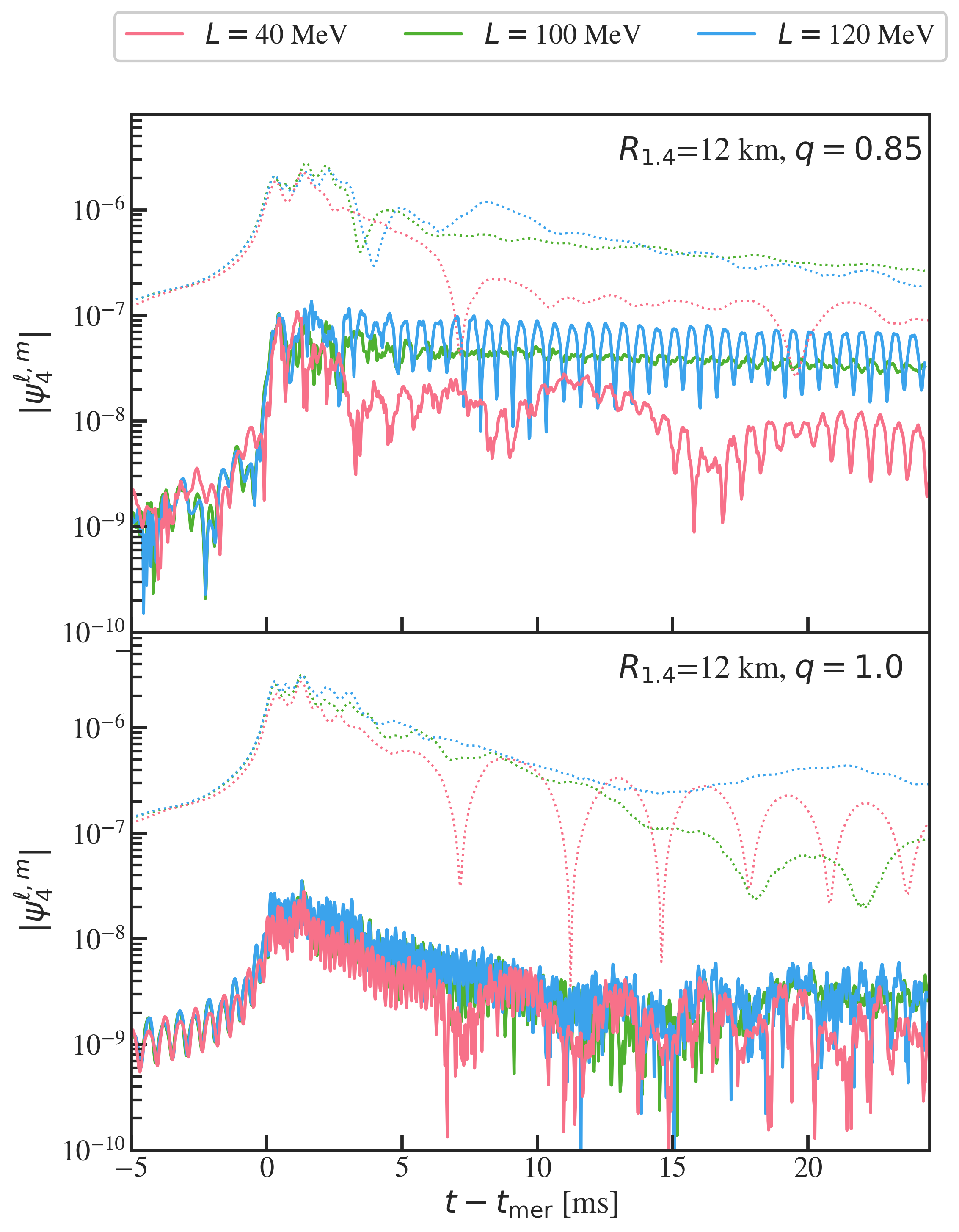
Figure 14: Amplitude of the spherical harmonic components of the GW signal for an edge-on merger at 40 Mpc, for the $R_{1.4}=12$ km EoSs. The solid and dotted lines correspond to the $(\ell,m)=(2,1)$ and (2,2) modes, respectively. For the $q=0.85$ binary (top panel), we find that the $m=1$ mode saturates within a few milliseconds of merger for the values of $L>100$ MeV, but that the $m=1$ mode quickly decays for the $L=40$ MeV EoS, indicating that this binary is rapidly becoming axisymmetric. In contrast, for the equal-mass binaries (bottom panel), the $m=1$ mode is in general weaker, and decays quickly for all values of $L$.

For the $R_{1.4}=12$ km, $L=40$ MeV EoS, Fig. 14 shows that the $m=1$ mode decays more quickly than any of the other, unequal-mass binaries. This is matched by a more rapid decay of $\psi_{4}^{2,2}$ in the same figure, as well as in the overall decay of the GW strain seen in Fig. 8. This damping of the GW emission suggests that the remnant quickly becomes axisymmetric. Indeed, the density contours in Fig. 4 show that the $R_{1.4}=12$ km, $L=40$ MeV EoS is nearly axisymmetric, while the $L=100$ and 120 MeV EoSs still show a strong $m=1$ deformation at late times. We conjecture that this rapid axisymmetrization may be related to the extreme stiffening of this particular EoS. We leave further exploration of this finding to future work.

IV Discussion and Conclusions

In this work we have investigated the impact of systematically varying the slope $L$ of the nuclear symmetry energy on the post-merger dynamics, mass ejection, and gravitational wave emission of a binary neutron star coalescence. We have considered seven new EoSs, which were constructed to have $R_{1.4}\,\simeq\,11$ km (with identical $\Lambda_{1.4}$), or $R_{1.4}=\,12\,,13\,\rm km$, and to vary systematically in $L$ from 40 to 120 MeV.

Concerning the properties of the post-merger remnant, we have found that for our baseline models with $R_{1.4}\,=\,12\,\rm km$ varying the slope of $L$ significantly affects the temperatures probed in the remnant. In particular, we found that the EoS with $R_{1.4}=12$ km, $L=40$ MeV reaches lower temperatures $T\,\lesssim\,40\,\rm MeV$ in the post-merger phase, whereas larger values of $L>100$ MeV for the same radius can reach $T\,\gtrsim\,60\,\rm MeV$. While the exact temperatures reached in the post-merger remnant are expected to also strongly depend on the total mass of the binary and the mass ratio, our results reported here are representative for a GW170817-like event and indicate a new sensitivity of the post-merger phase to the underlying EoS.

This increase in temperature for large $L$ can be understood in terms of the compressibility of the EoS around $n_{\rm sat}$. High temperatures in a merger are only produced during the post-merger bounces of the neutron star cores. These bounces drive compressions of the outer layers of the stars and, as a result, should correlate strongly with the radii of the stars. To be more precise, we find that the temperatures probed during the merger itself are inversely proportional to $R_{1.4}$, whereas the late-time temperatures in the remnant are more correlated (still inverse-proportionally) to $R_{1.8}$. Same concern as in the results; this does not correlate well with R1.8.

We have also found that the post-merger remnant becomes more rapidly axisymmetric for the $R_{1.4}=12$ km, $L=40$ MeV EoS, compared to EoSs with identical $R_{1.4}$ and larger $L$. In particular, we found that the $m=1$ deformation that is naturally induced in an asymmetric merger, e.g. with mass ratio $q=0.85$ considered here, is rapidly dampened for this small $L$ EoS. We do not find evidence of a similar damping in any other EoS we studied, including the $R_{1.4}\simeq 11$ km, $L=40$ MeV EoS; leading us to conjecture that the effect may in fact stem from the high-density EoS, rather than the specific value of $L$. Further studies with additional EoSs will be needed to clarify this behaviour.

Since post-merger gravitational wave signals are very promising probes of the dense matter EoS Baiotti and Rezzolla (2017); Paschalidis and Stergioulas (2017); Bauswein and Stergioulas (2019); Bernuzzi (2020); Radice et al. (2020), we also performed a detailed analysis of the GW emission extracted from our simulations. Interestingly, we found that the $R_{1.4}\,=\,12\rm km$ EoSs exhibit significantly different post-merger GW emission for the three values of $L$, which may be distinguishable with Advanced LIGO at design sensitivity. In particular, we found that for the EoSs with $R_{1.4}=12$ km, the $L=40$ MeV and $L=100$ MeV EoSs differ in $f_{2}$ by more than 300 Hz for both equal- and unequal-mass binaries, and differ by nearly 500 Hz for the $L=40$ MeV EoS compared to the $L=120$ MeV EoS.

In contrast, for the $R_{1.4}\simeq 11$ km EoSs, we found no significant differences in the post-merger GWs between the $L=40$ and 100 MeV cases, and we found only minor differences between the $R_{1.4}=13$ km EoSs, strongly hinting that $L$ is not uniquely imprinted in the gravitational wave signal. More precisely, whereas $L$ governs the behavior of the EoS around $n_{\rm sat}$, our findings suggest that the large differences in these EoSs at densities above $2\,n_{\rm sat}$ might be playing a stronger role in the dynamics of the post-merger system.

To further illustrate this point, we compared the results from our post-merger GW spectra to known quasi-universal relations that relate the post-merger peak frequencies to the neutron star radius Vretinaris et al. (2020) and found that using the standard relations to map from $f_{2}$ to the $R_{1.6}$ can lead to errors in the inferred radii of up to $\sim 1$ km, for the EoSs considered in this work. As shown in Fig. 11, we found that while the correlation between $f_{2}$ and $R_{1.4}$ is weak, a better result may be obtained by comparing $f_{2}$ with either the radius at higher masses, $R_{1.8}$, or by correlating $f_{2}$ with the pressure at $3n_{\rm sat}$. This underscores the importance of the high-density EoS, rather than $L$, in governing the post-merger GW spectrum.

Finally, we also considered the dynamical ejection of matter during the merger. Since this material is ejected from the outer parts of the star, we expect to here find the strongest correlation with $L$, as $L$ affects the EoS around $n_{\rm sat}$. Indeed, or the $q=0.85$ binaries, we found that smaller values of $L$ lead to a systematic (and monotonic) reduction in mass ejection (Tab. 2), with a corresponding, systematic increase in shock heating (Fig. 7). However, this trend is less clear in the subset of equal-mass binaries. In contrast, the compositional properties of the ejecta are similar in all cases and we only find minor differences in the fast tails of the ejecta velocities. Although only indicative at this point, due to the limited set of EoS and mass ratios considered here, we plan to follow up on these potential trends with $L$ in future works. This preliminary correlation between $L$ and the mass ejected may have implications on the feasibility of such systems to produce an X-ray and radio rebrightening years after the merger, as has recently been suggested for GW170817 Hajela et al. (2021); Balasubramanian et al. (2021), and may provide a new pathway for constraining the slope of the nuclear symmetry energy from observations of future electromagnetic counterparts. Determining the feasibility of such constraints, and the precise dependence on the mass ratio, will be the focus of future work.

Thus, although the post-merger dynamics and GWs do not show a clear signatures of the slope of the nuclear symmetry energy, we find a potential new correlation between $L$ and several properties of the dynamical ejecta. Our work also showcases the need for targeted EoS modelling, to systematically vary nuclear matter parameters while keeping the finite-temperature part of the EoS fixed, as was utilized in this study. Such targeted modelling will be crucial for better understanding systematic variations in the $f_{2}-R$ universal relations, as well as the differences in symmetrization timescales for post-merger remnants with different EoSs. Systematic construction of new EoSs will also allow us to follow-up on the tantalizing trends uncovered in this work, between $L$ and the properties of the dynamical ejecta, which may one day allow for new, astrophysical on the nuclear symmetry energy.

Appendix A Low-density symmetry energy

At densities below 0.5$n_{\rm sat}$, nuclei start to form and the nuclear symmetry energy expansion formalism breaks down. Accordingly, we start the transition from our analytic, high-density EoSs to a tabulated low-density EoS at $n=0.5n_{\rm sat}$, as described in Sec. II.1. However, across the transition window, between $6.3\times 10^{-5}$ and 0.08 fm^-3, the total energy is given by a combination of the tabulated EoS and the analytic model. In this regime, we therefore need a reasonable extrapolation of the symmetry energy model to combine with the low-density EoS table. In this appendix, we describe the treatment of the symmetry energy in this low-density regime.

We empirically choose a power-law decay model for the symmetry energy extrapolation, to ensure that $E_{\rm sym}$ (1) remains positive and real, (2) provides a diminishing contribution to the overall energy, and (3) predicts $Y_{e,\beta}\in(0,0.5]$, with $Y_{e,\beta}$ approaching that of SFHo at low densities.

For $n<0.5n_{\rm sat}$, we thus adopt the following model for the symmetry energy,

$$E_{\rm sym,low}(n)=[1-\chi(n)]E_{\rm fl}+\chi(n)E_{\rm PL}(n)$$ (8)

where $E_{\rm PL}(n)$ is a power-law function and $E_{\rm fl}$ is an energy floor that we set to 11.22 MeV. This floor corresponds to $E_{\rm sym}(0.5n_{\rm sat})/2$, calculated with the best-fit parameters for the SFHo EOS ($S=31.47$ MeV, $L=47.10$ MeV, $\gamma=0.41$; Raithel et al. (2019)). In this expression, $\chi(n)$ is a smoothing function that we define as

$$\chi(n)=\frac{1+\tanh\left[X\left(n-n_{0}\right)\right]}{2},$$ (9)

where we choose $X=40$ and $n_{0}=0.025$ fm^-3, such that $\chi(n)\approx 1$ at $0.5n_{\rm sat}$ (to within 1% accuracy), and $\chi(n)$ decreases at lower densities. These parameters and the value of $E_{\rm fl}$ were empirically chosen to ensure $Y_{p,\beta}(n)$ approximately matches that of SFHo across this density regime, for the EoSs explored in this work.

In order to ensure continuity in the symmetry energy and the corresponding pressure, we define the power-law energy extrapolation according to

$$E_{\rm PL}(n)=E_{\rm sym}(n_{t})+\frac{P_{\rm sym}(n_{t})}{n_{t}(\gamma_{\rm PL}-1)}\left[\left(\frac{n}{n_{t}}\right)^{\gamma_{\rm PL}-1}-1\right],$$ (10)

where $n_{t}=0.5n_{\rm sat}$, the power-law index is given by

$$\gamma_{\rm PL}=\frac{\partial P_{\rm sym}(n)}{\partial n}\biggr{\rvert}_{n_{t}}\left[\frac{n_{t}}{P_{\rm sym}(n_{t})}\right],$$ (11)

and $P_{\rm sym}(n)=n^{2}\partial E_{\rm sym}(n)/\partial n$.

In calculating the corresponding model for the low-density symmetry pressure, we neglect the density-derivatives of $\chi(n)$, which introduce unphysical density-dependences. Instead, we calculate the pressure in the two asymptotic limits, and use $\chi(n)$ to smoothly connect these regimes, i.e.,

$$P_{\rm sym,low}(n) =n^{2}\left(\frac{\partial E_{\rm fl}}{\partial n}\right)[1-\chi(n)]+n^{2}\left(\frac{\partial E_{\rm PL}(n)}{\partial n}\right)\chi(n)$$ (12)

$$=P_{\rm PL}(n)\chi(n)$$

where the first term disappears because $E_{\rm fl}$ is a constant and the remaining term is given simply by

$$P_{\rm PL}(n)=P_{\rm sym}(n_{t})\left(\frac{n}{n_{t}}\right)^{\gamma_{\rm PL}}.$$ (13)

Appendix B Chemical potentials

In this appendix, we describe the calculation of the chemical potentials, which are used to determine the neutrino transport opacities within our numerical evolutions (following Appendix A of Ruffert et al. (1996b)).

Because chemical potentials cannot be straightforwardly calculated within the original $M^{*}$-framework of Ref. Raithel et al. (2019), we here introduce an approximate calculation for the chemical potentials. We take advantage of the fact that the neutrino opacities depend primarily on the difference between the nucleon chemical potentials,

$$\hat{\mu}(n,Y_{p},T)\equiv\mu_{n}(n,Y_{p},T)-\mu_{p}(n,Y_{p},T),$$ (14)

where $\mu_{n}$ and $\mu_{p}$ are the neutron and proton chemical potentials, respectively. The individual nucleon potentials, $\mu_{n}$ and $\mu_{p}$, do not enter the calculation of the absorption opacities, and they enter the scattering opacity only via a term that accounts for Pauli blocking among the degenerate nucleons Ruffert et al. (1996b). Moreover, because Pauli blocking is relevant only at high densities, where the bulk of the matter is already expected to be optically thick to neutrino transport (e.g., Endrizzi et al., 2020), we do not expect the exact treatment of $\mu_{n}$ and $\mu_{p}$ to significantly affect the final optical depth of the remnant, as long as $\hat{\mu}$ is modeled accurately.

We, therefore, construct a self-consistent model for $\hat{\mu}$ at high-densities, based on the nuclear symmetry energy model used throughout this paper. We then define the individual chemical potentials relative to the values from the SFHo EoS table, such that $\mu_{n}(n,Y_{p},T)=\mu_{n,\rm{SFHO}}(n,Y_{p},T)$ and $\mu_{p}(n,Y_{p},T)\equiv\mu_{n,\rm{SFHO}}(n,Y_{p},T)-\hat{\mu}(n,Y_{p},T)$. Because we are already matching to the full SFHo table at low densities, using this EoS provides maximum consistency in our calculations. We again stress that this is mostly done for convenience with respect to the existing numerical infrastructure. Except for Pauli-blocking, the values for $\mu_{n}$ and $\mu_{p}$ never enter separately in our simulations. Furthermore, $\beta-$equilibrium is solely determined by the difference, $\hat{\mu}$.

We calculate $\hat{\mu}$ from the symmetry energy as follows. The chemical potential of species $i$ is defined as

$$\mu_{i}\equiv\frac{\partial E_{i}}{\partial Y_{i}}\biggr{\rvert}_{S,n}$$ (15)

where $E_{i}$ is the energy per baryon of that species, $Y_{i}$ is the corresponding number fraction, and $S$ is the entropy. For uniform $n$-$p$-$e$ matter, this implies

$$\frac{\partial E_{\rm tot}(n,Y_{p})}{\partial Y_{p}}=\mu_{p}+\mu_{e}-\mu_{n},$$ (16)

where $E_{\rm tot}$ represents the total energy, including contributions from neutrons, protons, and electrons. We have here assumed charge neutrality and conservation of baryon number, which require that $Y_{e}=Y_{p}$ and $Y_{p}=1-Y_{n}$, respectively. As in eq. (2), the total energy for zero-temperature $n$-$p$-$e$ matter can also be written in terms of the symmetric matter energy and a symmetry energy correction, i.e.,

$$E_{\rm tot}(n,Y_{p},T=0)=E_{0}(n)+E_{\rm sym}(n)(1-2Y_{p})^{2}+E_{e}(n,Y_{e}),$$ (17)

where we have additionally included the energy contribution from electrons, $E_{e}(n,Y_{e})$. Differentiating with respect to $Y_{p}$, we find

$$\frac{\partial E_{\rm tot}(n,Y_{p},T=0)}{\partial Y_{p}}=-4(1-2Y_{p})E_{\rm sym}(n)+\mu_{e}.$$ (18)

Combining eqs. (16) and (18), the zero-temperature difference in chemical potentials for neutrons and protons is then

$$\hat{\mu}(T=0)=4(1-2Y_{p})E_{\rm sym}(n).$$ (19)

Equation (19) thus ensures that $\hat{\mu}$ is consistent with the complete EoS model, for a given set of $E_{\rm sym}$ parameters. We note that this approach assumes that the thermal part of the chemical potential is the same for neutrons and protons. While this is an approximation, it is consistent with the overall decomposition of thermal effects from composition-dependent effects in the EoS framework of Ref. Raithel et al. (2019), where it was found that adding in the composition correction to the thermal model had a negligible effect on the total energy of the EoS (see Raithel et al. (2019) for further discussion).

Finally, we use the tabulated values from SFHo for the electron chemical potentials, which are simply given by the normal chemical potential for the Fermi-Dirac distribution function Hempel and Schaffner-Bielich (2010).

We reiterate that, on the short timescales ($\sim 25$ ms) considered in this paper, the high-density matter is expected to remain optically thick to neutrinos Endrizzi et al. (2020). Thus, we do not expect this high-density approximation for the chemical potentials to affect the outcomes of our evolutions or any of the conclusions in this paper. However, for longer-term evolutions, for example to simulate cooling of the neutron star remnant, this approximation may not be sufficient and should be further tested before use.

Appendix C Details on the gravitational wave analysis

Finally, in this appendix, we detail our methods for analyzing the GW emission. We extract the GW signal from our simulations using the Newman-Penrose scalar $\psi_{4}$, which is related to the GW strain according to $\psi_{4}=\ddot{h}_{+}-i\ddot{h}_{\times}$, where $h_{+}$ and $h_{\times}$ are the plus- and cross-polarizations of the GW strain and the dots indicate derivatives with respect to time. We decompose $\psi_{4}$ into $s=-2$ spin-weighted spherical harmonics on spheres of large radius ($r=300~{}M_{\odot}$), according to

$$\psi_{4}(t^{\prime\prime},r,\theta,\phi)=\sum_{\ell=2}^{\infty}\sum_{m=-\ell}^{\infty}\psi_{4}^{\ell,m}(t,r)_{-2}Y_{\ell,m}(\theta,\phi)$$ (20)

where $t$ is the time and the angles $\theta$ and $\phi$ are defined with respect to the angular momentum axis. The total strain is then given by

$$h(t) \equiv h_{+}-ih_{\times}$$ (21)

$$=\int_{-\infty}^{t}dt^{\prime}\int_{-\infty}^{t^{\prime}}dt^{\prime\prime}\psi_{4}(t^{\prime\prime},r,\theta,\phi),$$

where to calculate the double time integral, we use the fixed frequency integration (FFI) method of Reisswig and Pollney (2011).

In order to study the spectral features of the post-merger signals, we additionally calculate the characteristic strain, which is conventionally defined as

$$h_{c}(f)=2f\tilde{h}(f),$$ (22)

where $f$ is the frequency and $\tilde{h}(f)$ is the Fourier transform of $h(t)$ Moore et al. (2015) To calculate $\tilde{h}(f)$, we first window $\psi_{4}(t)$ between $t_{\rm mer}+1.5$ ms and the maximum time evolved for the binaries used in a particular comparison. We start the window shortly after $t_{\rm mer}$ in order to exclude the turbulent merger phase from the resulting spectra. For example, the $R_{1.4}\simeq 11$ km, $L=40$ MeV EoS collapsed after $\sim 15$ ms. Thus, in the following spectral comparisons of the $R_{1.4}\simeq 11$ km EoSs, we window both EoSs to the $\sim$14 ms window following merger, to ensure they have the same spectral resolution. For all other EoSs, the remnants do not collapse until the end of the evolution, so the windows are typically $\sim 24$ ms. We then compute the Fourier transform of the windowed $\psi_{4}(t)$, using Welch’s method with 8 overlapping segments for the longer-duration signals, and 7 overlapping segments for the $R_{1.4}\simeq 11$ km EoSs. Each segment is windowed with a Hann window and zero-padded to contain a total of 4,096 points. From $\tilde{\psi}_{4}(f)$, we then calculate $\tilde{h}(f)$, using the FFI technique of Reisswig and Pollney (2011). In this paper, we calculate $h_{c}(f)$ including all $\ell=2,3$ modes.

Finally, we calculate the distinguishability of the post-merger GW signals using the overlap integral Lindblom et al. (2008); McWilliams et al. (2010), defined as

$$O(h_{1},h_{2})=\frac{\left<h_{1},h_{2}\right>}{\sqrt{\left<h_{1},h_{1}\right>\left<h_{2},h_{2}\right>}},$$ (23)

where $\left<h_{i},h_{j}\right>$ is the inner product of two waveforms, given by

$$\left<h_{i},h_{j}\right>=4\mathrm{Re}\int_{f_{\rm min}}^{f_{\rm max}}\frac{\tilde{h}_{i}(f)\tilde{h}_{j}^{*}(f)}{S_{n}(f)}df,$$ (24)

$S_{n}(f)$ is the power spectral noise of the detector, and ^∗ indicates the complex conjugate. For the noise curve, we use the design sensitivity curve for Advanced LIGO Aasi et al. (2015), bounded between frequencies $f_{\rm min}$=1000 Hz and $f_{\rm max}=5000$ Hz. Values of the overlap integral smaller than $1-1/(2\rho^{2})$ are distinguishable, where $\rho$ is the signal-to-noise ratio (SNR). We consider the threshold SNR for detectability to be 8, in which case the criteria for distinguishability is $O\lesssim 0.992$.

References

- Piekarewicz and Centelles (2009) J. Piekarewicz and M. Centelles, Phys. Rev. C 79, 054311 (2009), eprint 0812.4499.
- Tsang et al. (2012) M. B. Tsang et al., Phys. Rev. C 86, 015803 (2012), eprint 1204.0466.
- Lattimer and Lim (2013) J. M. Lattimer and Y. Lim, Astrophys. J. 771, 51 (2013), eprint 1203.4286.
- Oertel et al. (2017) M. Oertel, M. Hempel, T. Klähn, and S. Typel, Rev. Mod. Phys. 89, 015007 (2017), eprint 1610.03361.
- Abrahamyan et al. (2012) S. Abrahamyan et al., Phys. Rev. Lett. 108, 112502 (2012), eprint 1201.2568.
- Horowitz et al. (2012) C. J. Horowitz et al., Phys. Rev. C 85, 032501 (2012), eprint 1202.1468.
- Adhikari et al. (2021) D. Adhikari et al. (PREX), Phys. Rev. Lett. 126, 172502 (2021), eprint 2102.10767.
- Reed et al. (2021) B. T. Reed, F. J. Fattoyev, C. J. Horowitz, and J. Piekarewicz, Phys. Rev. Lett. 126, 172503 (2021), eprint 2101.03193.
- Li et al. (2021) B.-A. Li, B.-J. Cai, W.-J. Xie, and N.-B. Zhang, Universe 7, 182 (2021), eprint 2105.04629.
- Lattimer and Prakash (2001) J. M. Lattimer and M. Prakash, Astrophys. J. 550, 426 (2001), eprint astro-ph/0002232.
- Yagi and Yunes (2013) K. Yagi and N. Yunes, Phys. Rev. D 88, 023009 (2013), eprint 1303.1528.
- Yagi and Yunes (2016) K. Yagi and N. Yunes, Class. Quant. Grav. 33, 13LT01 (2016), eprint 1512.02639.
- De et al. (2018) S. De, D. Finstad, J. M. Lattimer, D. A. Brown, E. Berger, and C. M. Biwer, Phys. Rev. Lett. 121, 091102 (2018), [Erratum: Phys.Rev.Lett. 121, 259902 (2018)], eprint 1804.08583.
- Raithel et al. (2018) C. Raithel, F. Özel, and D. Psaltis, Astrophys. J. Lett. 857, L23 (2018), eprint 1803.07687.
- Fattoyev et al. (2014) F. J. Fattoyev, W. G. Newton, and B.-A. Li, Eur. Phys. J. A 50, 45 (2014), eprint 1309.5153.
- Raithel et al. (2016) C. A. Raithel, F. Ozel, and D. Psaltis, Astrophys. J. 831, 44 (2016), eprint 1605.03591.
- Alam et al. (2016) N. Alam, B. K. Agrawal, M. Fortin, H. Pais, C. Providência, A. R. Raduta, and A. Sulaksono, Phys. Rev. C 94, 052801 (2016), eprint 1610.06344.
- Abbott et al. (2017a) B. P. Abbott et al. (LIGO Scientific, Virgo), Phys. Rev. Lett. 119, 161101 (2017a), eprint 1710.05832.
- Abbott et al. (2019a) B. P. Abbott et al. (LIGO Scientific, Virgo), Phys. Rev. X 9, 011001 (2019a), eprint 1805.11579.
- Krastev and Li (2019) P. G. Krastev and B.-A. Li, J. Phys. G 46, 074001 (2019), eprint 1801.04620.
- Malik et al. (2018) T. Malik, N. Alam, M. Fortin, C. Providência, B. K. Agrawal, T. K. Jha, B. Kumar, and S. K. Patra, Phys. Rev. C 98, 035804 (2018), eprint 1805.11963.
- Carson et al. (2019) Z. Carson, A. W. Steiner, and K. Yagi, Phys. Rev. D 99, 043010 (2019), eprint 1812.08910.
- Raithel and Ozel (2019) C. A. Raithel and F. Ozel (2019), eprint 1908.00018.
- Zhang and Li (2019) N.-B. Zhang and B.-A. Li, Eur. Phys. J. A 55, 39 (2019), eprint 1807.07698.
- Tsang et al. (2019) C. Y. Tsang, M. B. Tsang, P. Danielewicz, W. G. Lynch, and F. J. Fattoyev (2019), eprint 1901.07673.
- Essick et al. (2021) R. Essick, I. Tews, P. Landry, and A. Schwenk (2021), eprint 2102.10074.
- Baiotti and Rezzolla (2017) L. Baiotti and L. Rezzolla, Rept. Prog. Phys. 80, 096901 (2017), eprint 1607.03540.
- Paschalidis and Stergioulas (2017) V. Paschalidis and N. Stergioulas, Living Rev. Rel. 20, 7 (2017), eprint 1612.03050.
- Bauswein and Stergioulas (2019) A. Bauswein and N. Stergioulas, J. Phys. G 46, 113002 (2019), eprint 1901.06969.
- Bernuzzi (2020) S. Bernuzzi, Gen. Rel. Grav. 52, 108 (2020), eprint 2004.06419.
- Radice et al. (2020) D. Radice, S. Bernuzzi, and A. Perego, Ann. Rev. Nucl. Part. Sci. 70, 95 (2020), eprint 2002.03863.
- Bauswein et al. (2010) A. Bauswein, H. T. Janka, and R. Oechslin, Phys. Rev. D 82, 084043 (2010), eprint 1006.3315.
- Raithel et al. (2021) C. A. Raithel, V. Paschalidis, and F. Özel (2021), eprint 2104.07226.
- Metzger (2020) B. D. Metzger, Living Rev. Rel. 23, 1 (2020), eprint 1910.01617.
- Radice et al. (2018) D. Radice, A. Perego, K. Hotokezaka, S. A. Fromm, S. Bernuzzi, and L. F. Roberts, Astrophys. J. 869, 130 (2018), eprint 1809.11161.
- Kawaguchi et al. (2019) K. Kawaguchi, M. Shibata, and M. Tanaka (2019), eprint 1908.05815.
- Shibata and Hotokezaka (2019) M. Shibata and K. Hotokezaka, Ann. Rev. Nucl. Part. Sci. 69, 41 (2019), eprint 1908.02350.
- Raithel et al. (2019) C. A. Raithel, F. Ozel, and D. Psaltis, Astrophys. J. 875, 12 (2019), eprint 1902.10735.
- Steiner et al. (2013a) A. W. Steiner, M. Hempel, and T. Fischer, Astrophys. J. 774, 17 (2013a), eprint 1207.2184.
- Hotokezaka et al. (2018) K. Hotokezaka, K. Kiuchi, M. Shibata, E. Nakar, and T. Piran, Astrophys. J. 867, 95 (2018), eprint 1803.00599.
- Hajela et al. (2021) A. Hajela et al. (2021), eprint 2104.02070.
- Balasubramanian et al. (2021) A. Balasubramanian, A. Corsi, K. P. Mooley, M. Brightman, G. Hallinan, K. Hotokezaka, D. L. Kaplan, D. Lazzati, and E. J. Murphy, Astrophys. J. Lett. 914, L20 (2021), eprint 2103.04821.
- Steiner et al. (2013b) A. W. Steiner, M. Hempel, and T. Fischer, Astrophys. J. 774, 17 (2013b), eprint 1207.2184.
- Hempel and Schaffner-Bielich (2010) M. Hempel and J. Schaffner-Bielich, Nucl. Phys. A 837, 210 (2010), eprint 0911.4073.
- Ozel and Psaltis (2009) F. Ozel and D. Psaltis, Phys. Rev. D 80, 103003 (2009), eprint 0905.1959.
- Read et al. (2009) J. S. Read, B. D. Lackey, B. J. Owen, and J. L. Friedman, Phys. Rev. D 79, 124032 (2009), eprint 0812.2163.
- Steiner et al. (2010) A. W. Steiner, J. M. Lattimer, and E. F. Brown, Astrophys. J. 722, 33 (2010), eprint 1005.0811.
- Demorest et al. (2010) P. Demorest, T. Pennucci, S. Ransom, M. Roberts, and J. Hessels, Nature 467, 1081 (2010), eprint 1010.5788.
- Antoniadis et al. (2013) J. Antoniadis et al., Science 340, 6131 (2013), eprint 1304.6875.
- Fonseca et al. (2016) E. Fonseca et al., Astrophys. J. 832, 167 (2016), eprint 1603.00545.
- Cromartie et al. (2019) H. T. Cromartie et al. (NANOGrav), Nature Astron. 4, 72 (2019), eprint 1904.06759.
- Gandolfi et al. (2014) S. Gandolfi, J. Carlson, S. Reddy, A. W. Steiner, and R. B. Wiringa, Eur. Phys. J. A 50, 10 (2014), eprint 1307.5815.
- Ozel et al. (2016) F. Ozel, D. Psaltis, T. Guver, G. Baym, C. Heinke, and S. Guillot, Astrophys. J. 820, 28 (2016), eprint 1505.05155.
- Favata (2014) M. Favata, Phys. Rev. Lett. 112, 101101 (2014), eprint 1310.8288.
- Oechslin et al. (2007) R. Oechslin, H. T. Janka, and A. Marek, Astron. Astrophys. 467, 395 (2007), eprint astro-ph/0611047.
- Sekiguchi et al. (2011) Y. Sekiguchi, K. Kiuchi, K. Kyutoku, and M. Shibata, Phys. Rev. Lett. 107, 051102 (2011), eprint 1105.2125.
- Bernuzzi et al. (2016) S. Bernuzzi, D. Radice, C. D. Ott, L. F. Roberts, P. Moesta, and F. Galeazzi, Phys. Rev. D 94, 024023 (2016), eprint 1512.06397.
- Perego et al. (2019) A. Perego, S. Bernuzzi, and D. Radice, Eur. Phys. J. A 55, 124 (2019), eprint 1903.07898.
- Schneider et al. (2017) A. S. Schneider, L. F. Roberts, and C. D. Ott, Phys. Rev. C 96, 065802 (2017), eprint 1707.01527.
- Most et al. (2019a) E. R. Most, L. J. Papenfort, V. Dexheimer, M. Hanauske, S. Schramm, H. Stöcker, and L. Rezzolla, Phys. Rev. Lett. 122, 061101 (2019a), eprint 1807.03684.
- Hilditch et al. (2013) D. Hilditch, S. Bernuzzi, M. Thierfelder, Z. Cao, W. Tichy, and B. Bruegmann, Phys. Rev. D 88, 084057 (2013), eprint 1212.2901.
- Bernuzzi and Hilditch (2010) S. Bernuzzi and D. Hilditch, Phys. Rev. D 81, 084003 (2010), eprint 0912.2920.
- Bona et al. (2003) C. Bona, T. Ledvinka, C. Palenzuela, and M. Zacek, Phys. Rev. D 67, 104005 (2003), eprint gr-qc/0302083.
- Gundlach et al. (2005) C. Gundlach, J. M. Martin-Garcia, G. Calabrese, and I. Hinder, Class. Quant. Grav. 22, 3767 (2005), eprint gr-qc/0504114.
- Weyhausen et al. (2012) A. Weyhausen, S. Bernuzzi, and D. Hilditch, Phys. Rev. D 85, 024038 (2012), eprint 1107.5539.
- Alcubierre et al. (2003) M. Alcubierre, B. Bruegmann, P. Diener, M. Koppitz, D. Pollney, E. Seidel, and R. Takahashi, Phys. Rev. D 67, 084023 (2003), eprint gr-qc/0206072.
- Schnetter (2010) E. Schnetter, Class. Quant. Grav. 27, 167001 (2010), eprint 1003.0859.
- Babiuc et al. (2008) M. C. Babiuc et al., Class. Quant. Grav. 25, 125012 (2008), eprint 0709.3559.
- Duez et al. (2005) M. D. Duez, Y. T. Liu, S. L. Shapiro, and B. C. Stephens, Phys. Rev. D 72, 024028 (2005), eprint astro-ph/0503420.
- Shibata and Sekiguchi (2005) M. Shibata and Y.-i. Sekiguchi, Phys. Rev. D 72, 044014 (2005), eprint astro-ph/0507383.
- Ruffert et al. (1996a) M. H. Ruffert, H. T. Janka, and G. Schaefer, Astron. Astrophys. 311, 532 (1996a), eprint astro-ph/9509006.
- Rosswog and Liebendoerfer (2003) S. Rosswog and M. Liebendoerfer, Mon. Not. Roy. Astron. Soc. 342, 673 (2003), eprint astro-ph/0302301.
- Most et al. (2019b) E. R. Most, L. J. Papenfort, and L. Rezzolla, Mon. Not. Roy. Astron. Soc. 490, 3588 (2019b), eprint 1907.10328.
- Etienne et al. (2015) Z. B. Etienne, V. Paschalidis, R. Haas, P. Mösta, and S. L. Shapiro, Class. Quant. Grav. 32, 175009 (2015), eprint 1501.07276.
- Zlochower et al. (2005) Y. Zlochower, J. G. Baker, M. Campanelli, and C. O. Lousto, Phys. Rev. D 72, 024021 (2005), eprint gr-qc/0505055.
- Del Zanna et al. (2007) L. Del Zanna, O. Zanotti, N. Bucciantini, and P. Londrillo, Astron. Astrophys. 473, 11 (2007), eprint 0704.3206.
- Loffler et al. (2012) F. Loffler et al., Class. Quant. Grav. 29, 115001 (2012), eprint 1111.3344.
- Schnetter et al. (2004) E. Schnetter, S. H. Hawley, and I. Hawke, Class. Quant. Grav. 21, 1465 (2004), eprint gr-qc/0310042.
- Gourgoulhon et al. (2001) E. Gourgoulhon, P. Grandclement, K. Taniguchi, J.-A. Marck, and S. Bonazzola, Phys. Rev. D 63, 064029 (2001), eprint gr-qc/0007028.
- Abbott et al. (2017b) B. P. Abbott et al. (LIGO Scientific, Virgo), Phys. Rev. Lett. 119, 161101 (2017b), eprint 1710.05832.
- Abbott et al. (2019b) B. P. Abbott et al. (LIGO Scientific, Virgo), Phys. Rev. X 9, 011001 (2019b), eprint 1805.11579.
- Nedora et al. (2020) V. Nedora, F. Schianchi, S. Bernuzzi, D. Radice, B. Daszuta, A. Endrizzi, A. Perego, A. Prakash, and F. Zappa (2020), eprint 2011.11110.
- Hanauske et al. (2017) M. Hanauske, K. Takami, L. Bovard, L. Rezzolla, J. A. Font, F. Galeazzi, and H. Stöcker, Phys. Rev. D 96, 043004 (2017), eprint 1611.07152.
- Radice (2017) D. Radice, Astrophys. J. Lett. 838, L2 (2017), eprint 1703.02046.
- Shibata and Kiuchi (2017) M. Shibata and K. Kiuchi, Phys. Rev. D 95, 123003 (2017), eprint 1705.06142.
- Most et al. (2021) E. R. Most, S. P. Harris, C. Plumberg, M. G. Alford, J. Noronha, J. Noronha-Hostler, F. Pretorius, H. Witek, and N. Yunes (2021), eprint 2107.05094.
- Bauswein et al. (2013) A. Bauswein, S. Goriely, and H. T. Janka, Astrophys. J. 773, 78 (2013), eprint 1302.6530.
- Hanauske et al. (2019) M. Hanauske, J. Steinheimer, A. Motornenko, V. Vovchenko, L. Bovard, E. R. Most, L. J. Papenfort, S. Schramm, and H. Stöcker, Particles 2, 44 (2019).
- Most et al. (2020) E. R. Most, L. Jens Papenfort, V. Dexheimer, M. Hanauske, H. Stoecker, and L. Rezzolla, Eur. Phys. J. A 56, 59 (2020), eprint 1910.13893.
- Prakash et al. (2021) A. Prakash, D. Radice, D. Logoteta, A. Perego, V. Nedora, I. Bombaci, R. Kashyap, S. Bernuzzi, and A. Endrizzi (2021), eprint 2106.07885.
- Fujibayashi et al. (2017) S. Fujibayashi, Y. Sekiguchi, K. Kiuchi, and M. Shibata, Astrophys. J. 846, 114 (2017), eprint 1703.10191.
- Fujibayashi et al. (2018) S. Fujibayashi, K. Kiuchi, N. Nishimura, Y. Sekiguchi, and M. Shibata, Astrophys. J. 860, 64 (2018), eprint 1711.02093.
- Sekiguchi et al. (2016) Y. Sekiguchi, K. Kiuchi, K. Kyutoku, M. Shibata, and K. Taniguchi, Phys. Rev. D 93, 124046 (2016), eprint 1603.01918.
- Lehner et al. (2016a) L. Lehner, S. L. Liebling, C. Palenzuela, O. L. Caballero, E. O’Connor, M. Anderson, and D. Neilsen, Class. Quant. Grav. 33, 184002 (2016a), eprint 1603.00501.
- Bovard et al. (2017) L. Bovard, D. Martin, F. Guercilena, A. Arcones, L. Rezzolla, and O. Korobkin, Phys. Rev. D 96, 124005 (2017), eprint 1709.09630.
- Abbott et al. (2017c) B. P. Abbott et al. (LIGO Scientific, Virgo), Astrophys. J. Lett. 850, L39 (2017c), eprint 1710.05836.
- Nedora et al. (2021) V. Nedora, D. Radice, S. Bernuzzi, A. Perego, B. Daszuta, A. Endrizzi, A. Prakash, and F. Schianchi (2021), eprint 2104.04537.
- Bovard and Rezzolla (2017) L. Bovard and L. Rezzolla, Class. Quant. Grav. 34, 215005 (2017), eprint 1705.07882.
- Sekiguchi et al. (2015) Y. Sekiguchi, K. Kiuchi, K. Kyutoku, and M. Shibata, Phys. Rev. D 91, 064059 (2015), eprint 1502.06660.
- Foucart et al. (2018) F. Foucart, T. Hinderer, and S. Nissanke, Phys. Rev. D 98, 081501 (2018), eprint 1807.00011.
- Dietrich et al. (2021) T. Dietrich, T. Hinderer, and A. Samajdar, Gen. Rel. Grav. 53, 27 (2021), eprint 2004.02527.
- Metzger et al. (2015) B. D. Metzger, A. Bauswein, S. Goriely, and D. Kasen, Mon. Not. Roy. Astron. Soc. 446, 1115 (2015), eprint 1409.0544.
- Aasi et al. (2015) J. Aasi et al. (LIGO Scientific), Class. Quant. Grav. 32, 074001 (2015), eprint 1411.4547.
- Punturo et al. (2010) M. Punturo et al., Class. Quant. Grav. 27, 194002 (2010).
- Stergioulas et al. (2011) N. Stergioulas, A. Bauswein, K. Zagkouris, and H.-T. Janka, Mon. Not. Roy. Astron. Soc. 418, 427 (2011), eprint 1105.0368.
- Takami et al. (2014) K. Takami, L. Rezzolla, and L. Baiotti, Phys. Rev. Lett. 113, 091104 (2014), eprint 1403.5672.
- Lindblom et al. (2008) L. Lindblom, B. J. Owen, and D. A. Brown, Phys. Rev. D 78, 124020 (2008), eprint 0809.3844.
- McWilliams et al. (2010) S. T. McWilliams, B. J. Kelly, and J. G. Baker, Phys. Rev. D 82, 024014 (2010), eprint 1004.0961.
- Vretinaris et al. (2020) S. Vretinaris, N. Stergioulas, and A. Bauswein, Phys. Rev. D 101, 084039 (2020), eprint 1910.10856.
- Bauswein et al. (2012) A. Bauswein, H. T. Janka, K. Hebeler, and A. Schwenk, Phys. Rev. D 86, 063001 (2012), eprint 1204.1888.
- Chatziioannou et al. (2017) K. Chatziioannou, J. A. Clark, A. Bauswein, M. Millhouse, T. B. Littenberg, and N. Cornish, Phys. Rev. D 96, 124035 (2017), eprint 1711.00040.
- Breschi et al. (2019) M. Breschi, S. Bernuzzi, F. Zappa, M. Agathos, A. Perego, D. Radice, and A. Nagar, Phys. Rev. D 100, 104029 (2019), eprint 1908.11418.
- Bose et al. (2018) S. Bose, K. Chakravarti, L. Rezzolla, B. S. Sathyaprakash, and K. Takami, Phys. Rev. Lett. 120, 031102 (2018), eprint 1705.10850.
- Haster et al. (2020) C.-J. Haster, K. Chatziioannou, A. Bauswein, and J. A. Clark, Phys. Rev. Lett. 125, 261101 (2020), eprint 2004.11334.
- Shibata et al. (2019) M. Shibata, E. Zhou, K. Kiuchi, and S. Fujibayashi, Phys. Rev. D 100, 023015 (2019), eprint 1905.03656.
- Nathanail et al. (2021) A. Nathanail, E. R. Most, and L. Rezzolla, Astrophys. J. Lett. 908, L28 (2021), eprint 2101.01735.
- Zappa et al. (2018) F. Zappa, S. Bernuzzi, D. Radice, A. Perego, and T. Dietrich, Phys. Rev. Lett. 120, 111101 (2018), eprint 1712.04267.
- Paschalidis et al. (2015) V. Paschalidis, W. E. East, F. Pretorius, and S. L. Shapiro, Phys. Rev. D 92, 121502 (2015), eprint 1510.03432.
- East et al. (2016a) W. E. East, V. Paschalidis, F. Pretorius, and S. L. Shapiro, Phys. Rev. D 93, 024011 (2016a), eprint 1511.01093.
- East et al. (2016b) W. E. East, V. Paschalidis, and F. Pretorius, Class. Quant. Grav. 33, 244004 (2016b), eprint 1609.00725.
- Lehner et al. (2016b) L. Lehner, S. L. Liebling, C. Palenzuela, and P. M. Motl, Phys. Rev. D 94, 043003 (2016b), eprint 1605.02369.
- Radice et al. (2016) D. Radice, S. Bernuzzi, and C. D. Ott, Phys. Rev. D 94, 064011 (2016), eprint 1603.05726.
- Nedora et al. (2019) V. Nedora, S. Bernuzzi, D. Radice, A. Perego, A. Endrizzi, and N. Ortiz, Astrophys. J. Lett. 886, L30 (2019), eprint 1907.04872.
- Ruffert et al. (1996b) M. H. Ruffert, H. T. Janka, and G. Schaefer, Astron. Astrophys. 311, 532 (1996b), eprint astro-ph/9509006.
- Endrizzi et al. (2020) A. Endrizzi, A. Perego, F. M. Fabbri, L. Branca, D. Radice, S. Bernuzzi, B. Giacomazzo, F. Pederiva, and A. Lovato, Eur. Phys. J. A 56, 15 (2020), eprint 1908.04952.
- Reisswig and Pollney (2011) C. Reisswig and D. Pollney, Class. Quant. Grav. 28, 195015 (2011), eprint 1006.1632.
- Moore et al. (2015) C. J. Moore, R. H. Cole, and C. P. L. Berry, Class. Quant. Grav. 32, 015014 (2015), eprint 1408.0740.