Numerical Relativity Simulations of the Neutron Star Merger GW170817:
Long-Term Remnant Evolutions, Winds, Remnant Disks, and Nucleosynthesis

Abstract

We present a systematic numerical-relativity study of the dynamical ejecta, winds and nucleosynthesis in neutron star merger remnants. Binaries with the chirp mass compatible with GW170817, different mass ratios, and five microphysical equations of state (EOS) are simulated with an approximate neutrino transport and a subgrid model for magnetohydrodynamics turbulence up to $100$ milliseconds postmerger. Spiral density waves propagating from the neutron star remnant to the disk trigger a wind with mass flux ${\sim}0.1{-}0.5\,{\mathrm{M}_{\odot}}/s$ persisting for the entire simulation as long as the remnant does not collapse to black hole. This wind has average electron fraction $\gtrsim 0.3$ and average velocity ${\sim}0.1-0.17\,$c and thus is a site for the production of weak $r$-process elements (mass number $A<195$). Disks around long-lived remnants have masses ${\sim}0.1-0.2\,{\mathrm{M}_{\odot}}$, temperatures peaking at $\lesssim 10\,{\mathrm{M}eV}$ near the inner edge, and a characteristic double-peak distribution in entropy resulting from shocks propagating through the disk. The dynamical and spiral-wave ejecta computed in our targeted simulations are not compatible with those inferred from AT2017gfo using two-components kilonova models. Rather, they indicate that multi-component kilonova models including disk winds are necessary to interpret AT2017gfo. The nucleosynthesis in the combined dynamical ejecta and spiral-wave wind in the comparable-mass long-lived mergers robustly accounts for all the $r$-process peaks, from mass number ${\sim}75$ to actinides in terms of solar abundances. Total abundandes are weakly dependent on the EOS, while the mass ratio affect the production of first peak elements.

1. Introduction

The mass ejection of neutron-rich matter from binary neutron star (BNS) mergers has been theoretically studied since the ‘70s as a possible site for $r$-process nucleosynthesis (Lattimer & Schramm, 1974; Symbalisty & Schramm, 1982; Rosswog et al., 1999; Freiburghaus et al., 1999; Rosswog, 2005). The radioactive decay of $r$-process elements produces a characteristic electromagnetic (EM) transient in the UV/optical/NIR bands, called kilonova (kN) (Li & Paczynski, 1998; Kulkarni, 2005; Metzger et al., 2010; Roberts et al., 2011; Kasen et al., 2013), that was observed as counterpart of the gravitational-wave event GW170817 (Abbott et al., 2017a, b, 2019, 2018b) and it was named AT2017gfo (Arcavi et al., 2017; Coulter et al., 2017; Drout et al., 2017; Evans et al., 2017; Hallinan et al., 2017; Kasliwal et al., 2017; Nicholl et al., 2017; Smartt et al., 2017; Soares-Santos et al., 2017; Tanvir et al., 2017; Troja et al., 2017; Mooley et al., 2018; Ruan et al., 2018; Lyman et al., 2018). The NIR luminosity of AT2017gfo peaked at several days after the merger (Chornock et al., 2017), and it is consistent with the expectation that the opacities of expanding $r$-process material are dominated by lanthanides and possibly actinides (Kasen et al., 2013). The UV/optical luminosity peaked instead less than one day after the merger (Nicholl et al., 2017), and it originates from ejected material that experienced only a partial $r$-process nucleosynthesis (Martin et al., 2015).

The ejecta masses inferred from observations (Cowperthwaite et al., 2017; Villar et al., 2017; Tanvir et al., 2017; Tanaka et al., 2017; Perego et al., 2017; Kawaguchi et al., 2018) are not compatible with those predicted by numerical simulations with targeted neutron star (NS) masses, and several questions remain open. In particular, understanding the early blue kN remains a challenging aspect to most models. Both semi-analytical and radiation transport models require large ejecta velocities and electron fractions ($Y_{e}$’s), different from those found in simulations, (e.g., Fahlman & Fernández, 2018; Nedora et al., 2019). The late red kN component requires ejecta masses generally not observed for the dynamical ejecta computed in numerical relativity (NR) simulations (Radice et al., 2018b). In addition, the number of components and the geometry of the emission can have a significant effect on the ejecta parameters (Perego et al., 2017; Kawaguchi et al., 2018). Also, it is important to note that the photon diffusion and emission is often simplified in semi-analytical kN models (e.g., Villar et al., 2017; Perego et al., 2017; Siegel, 2019), and the more accurate radiation transfer computations may alter the inferred ejecta parameters (Kawaguchi et al., 2018; Korobkin et al., 2020). However, photon radiation transfer simulations often employ ad-hoc, simplified ejecta that are not computed from ab-initio simulations.

Key for interpreting BNS electromagnetic emissions is the detailed modeling of the mass ejection from BNS mergers, which must include general relativity, a microphysical equation of states (EOS) of strongly interacting matter, relativistic (magneto-)hydrodynamics, and neutrino transport. NR simulations performed so far mostly focused on the dynamical ejecta that are launched during merger by tidal torques (tidal component) and by the shocks generated by the bounce of the NS cores (shocked component), (e.g., Hotokezaka et al., 2013; Bauswein et al., 2013; Wanajo et al., 2014; Sekiguchi et al., 2015; Radice et al., 2016b; Sekiguchi et al., 2016; Radice et al., 2018b; Vincent et al., 2020). In equal-mass mergers, the shocked component is found to be a factor ${\sim}10$ more massive than the tidal component. This is in contrast to early works that employed Newtonian gravity and in which the tidal component dominated the ejecta due to the weaker gravity and stiffer EOS employed in those simulations (Ruffert et al., 1997; Rosswog et al., 1999; Rosswog & Davies, 2003; Rosswog & Liebendoerfer, 2003; Rosswog et al., 2003; Rosswog & Ramirez-Ruiz, 2003; Oechslin et al., 2006; Rosswog et al., 2014; Korobkin et al., 2012). However, even the dynamical ejecta found in NR simulations cannot account alone for the bright blue and late red components of the observed kN in AT2017gfo (Siegel, 2019).

Winds originating from the merger remnant on timescales of $\mathcal{O}(0.1-1\,{\mathrm{s}})$ can unbind $O(0.1\,{\mathrm{M}_{\odot}})$ from the remnant and represent (if present) the largest contribution to the kilonova signal (Dessart et al., 2009; Fernández et al., 2015; Just et al., 2015; Lippuner et al., 2017; Siegel & Metzger, 2017; Fujibayashi et al., 2018; Radice et al., 2018a; Fernández et al., 2019; Janiuk, 2019; Miller et al., 2019; Fujibayashi et al., 2020a; Mösta et al., 2020). Thus far, these winds have been mostly studied by means of long-term Newtonian simulations of neutrino-cooled disks, assuming simplified initial conditions, (Metzger et al., 2008; Beloborodov, 2008; Lee et al., 2009; Fernández & Metzger, 2013, e.g.,). Ab-initio (3+1)D NR simulations of the merger with weak-interactions and magnetohydrodynamics are not yet fully developed at sufficiently long timescales (Sekiguchi et al., 2011; Wanajo et al., 2014; Sekiguchi et al., 2015; Palenzuela et al., 2015; Radice et al., 2016b; Lehner et al., 2016a; Sekiguchi et al., 2016; Foucart et al., 2017; Bovard et al., 2017; Fujibayashi et al., 2018, 2017; Radice et al., 2018a; Nedora et al., 2019; Vincent et al., 2020; Bernuzzi et al., 2020). These simulations are essential to interpret AT2017gfo and future events. For example, long-term (up to $100$ ms postmerger) NR simulations pointed out the existence of spiral-wave wind in which there are favourable conditions (large ejecta mass, high-velocity and not extremely neutron rich conditions) for the early emission from lanthanide poor material (Nedora et al., 2019). Such mass ejection can also be boosted by global large-scale magnetic stresses (Metzger et al., 2018; Siegel & Metzger, 2018, 2017), although significant mass fluxes can only be achieved by fine-tuning initial configuration or setting unrealistic strength of the magnetic field (e.g., Ciolfi, 2020; Mösta et al., 2020). A third contribution can come from neutrino-driven winds of mass ${\sim}10^{-4}-10^{-3}M_{\odot}$ originating above the remnant, but their mass cannot account for bright signals (Dessart et al., 2009; Perego et al., 2014; Just et al., 2015).

The nucleosynthesis from BNS mergers is believed to provide a major contribution to the $r$-process material in the Universe. However, whether or not BNS mergers are the only source is still debated and possible additional $r$-process sites, such as collapsars, jet-driven supernovae, and neutron star implosions, have been proposed (Argast et al., 2004; Duan et al., 2011; Winteler et al., 2012; Nishimura et al., 2015; Hirai et al., 2015; Bramante & Linden, 2016; Nishimura et al., 2017; Fuller et al., 2017; Mösta et al., 2018; Siegel et al., 2018; Ji et al., 2019; Bartos & Marka, 2019; van de Voort et al., 2020; Wehmeyer et al., 2019; Vassh et al., 2020). In particular, it is not clear if BNS mergers can explain r-process enriched ultra-faint dwarf galaxies, classical dwarf galaxies (Ji et al., 2016; Bramante & Linden, 2016; Safarzadeh et al., 2019b, a; Skúladóttir, Ása and Hansen, Camilla Juul and Salvadori, Stefania and Choplin, Arthur, 2019; Bonetti et al., 2019), and the evolution of $r$-process abundances both at early and late times (Safarzadeh & Côté, 2017; Safarzadeh et al., 2019b; Bonetti et al., 2018; Côté et al., 2019; Hotokezaka et al., 2018; Banerjee et al., 2020)

In this work we address the problem of the remnant evolution on the viscous timescale by means of ab-initio (3+1)D NR simulations. We present new simulations performed with five microphysical EOS, a M0 neutrino transport scheme and a subgrid model for the magnetohydrodynamics turbulence. We compute dynamical ejecta and spiral-wave wind, and we calculate the nucleosynthesis of the resulting unbound mass. The simulations and analysis methods are detailed in Sec. 2. Section 3 gives an overview of the remnants dynamics, describing the main features in terms of the binary parameters. The properties of the dynamical ejecta are summarized in Sec. 4, where we compare with simple models for AT2017gfo. Sections 5 and 6 describe the mechanism powering the spiral-wave wind and $\nu$-component in long-lived remnants. This mechanism is a combination of $m=2$ and $m=1$ modes in the remnant powering spiral-density waves in the disk. A polar component of the spiral-wave wind is powered by neutrino heating above the remnant. The properties of the remnant disk, including thermodynamical quantities, are discussed in Sec. 7. The composition of the disk at the end of the simulations is charaterized by double peaks in the entropy and electron fraction profiles. Section 8 presents nucleosynthesis calculations on the combined dynamical and wind ejecta. The combined yields in the ejecta of long-lived remnants show a good fit to the solar abundance patterns for all $r-$process peaks. Throughout the text we discuss the implications of our results for AT2017gfo.

2. Methods

Within (3+1)D NR we solve the equations of general-relativistic hydrodynamics for a perfect fluid coupled to the Z4c free evolution scheme for Einstein’s equations (Bernuzzi & Hilditch, 2010; Hilditch et al., 2013). The interactions between the neutrinos radiation and the fluid are treated with a leakage scheme in the optically thick regions (Ruffert et al., 1996; Galeazzi et al., 2013; Neilsen et al., 2014) while free-streaming neutrinos are evolved according to the M0 scheme (Radice et al., 2018b). The effect of large-scale magnetic fields are simulated with the general-relativistic large eddy simulations method (GRLES) for turbulent viscosity (Radice, 2017).

2.1. Matter and radiation treatement

We write the fluid’s stress-energy tensor as

$$T_{\mu\nu}=\rho hu_{\mu}u_{\nu}+Pg_{\mu\nu}$$ (1)

where $\rho=m_{\mathrm{b}}n$ is the baryon rest-mass density, $n$ the baryon number density, $m_{\mathrm{b}}$ the baryonic mass, $h=1+\epsilon+P/\rho$ the specific enthalpy, $\epsilon$ the specific internal energy, $u^{\mu}$ the fluid 4-velocity and $P$ the pressure. The fluid satisfies the Euler’s equations:

$$\nabla_{\nu}T^{\mu\nu}=Qu^{\mu}\ ,$$ (2)

where $Q$ is the net energy exchange rate due to the absorption and emission of neutrinos, given by Eq. (11) of Radice et al. (2018b). The above system of equations is closed by a finite-temperature ($T$), composition-dependent EOS in the form $P=P(\rho,Y_{e},T)$, and by the evolution equations for the proton and neutron number densities:

$$\nabla_{\nu}(n_{p}u^{\mu})=R_{p}^{\mu}\ \ ,\ \ \nabla_{\nu}(n_{n}u^{\mu})=R_{n}^{\mu}\ .$$ (3)

where the total proton fraction is computed as $n_{p}=Y_{e}n$, $n_{p}+n_{n}=n$, and $R_{p}=-R_{n}$ is the net lepton number exchange rate due to the absorption and emission of neutrinos and anti-neutrinos.

We treat compositional and energy changes in the material due to weak reactions using the leakage scheme presented in Galeazzi et al. (2013); Radice et al. (2016b); see also van Riper & Lattimer (1981); Ruffert et al. (1996); Rosswog & Liebendoerfer (2003); O’Connor & Ott (2010); Sekiguchi (2010); Neilsen et al. (2014); Perego et al. (2016); Ardevol-Pulpillo et al. (2019); Gizzi et al. (2019) for other implementations. We track reactions involving electron neutrinos ($\nu_{e}$) and antineutrinos ($\bar{\nu}_{e}$) separately, and treat heavy-lepton neutrinos in a single effective species ($\nu_{x}$). The production rates $R_{\nu}$, $\nu\in\{\nu_{e},\bar{\nu}_{e},\nu_{x}\}$, the associated production energies $Q_{\nu}$, and neutrino absorption $\kappa_{\nu,a}$ and scattering $\kappa_{\nu,s}$ opacities are computed from the reactions listed in table 3 of Perego et al. (2019). Neutrinos are then split into a trapped component with number density $n_{\nu}^{\mathrm{t}rap}$ and a free-streaming component $n_{\nu}^{\mathrm{f}s}$. The latter are emitted according to the effective rate $R_{\nu}^{\mathrm{e}ff}$ (Ruffert et al., 1996) (see Radice et al., 2018b, Eq. (4)) and with average energy $Q_{\nu}^{\mathrm{e}ff}/R_{\nu}^{\mathrm{e}ff}$ and then evolved according to the M0 scheme of Radice et al. (2018b). The M0 scheme evolves the number density of the free-streaming neutrinos assuming that they move along radial null rays, and estimates the free-streaming neutrino energy, $E_{\nu}$, under the additional assumption of stationary metric. Note that the pressure due to the trapped neutrino component is neglected, since it is found to be important at a level $\lesssim 5\%$ in the conditions relevant for BNS mergers (Galeazzi et al., 2013; Perego et al., 2019).

Our simulations do not include magnetic fields but we simulate the angular momentum transport due to magnetohydrodynamics turbulence by using an effective viscosity and the GRLES scheme (Radice, 2017, 2020). The subgrid model employed in this work is described in Radice (2020), and it is designed based on the results of the high-resolution general relativistic magnetohydrodynamics simulations results of a BNS merger of Kiuchi et al. (2018). This GRLES subgrid model has been already used in Perego et al. (2019); Endrizzi et al. (2019); Nedora et al. (2019); Bernuzzi et al. (2020).

2.2. EOS models

We consider five different nuclear EOS models: BLh, DD2, LS220, SFHo and SLy4 (see Perego et al., 2019, table 1) where DD2, LS220 and SFHo are summarized). All these EOS include neutrons ($n$), protons ($p$), nuclei, electrons, positrons, and photons as relevant degrees of freedom. Cold, neutrino-less $\beta$-equilibrated matter described by these microphysical EOSs predicts NS maximum masses and radii within the range allowed by current astrophysical constraints, including the recent GW constraint on tidal deformability (Abbott et al., 2017c, 2019; De et al., 2018; Abbott et al., 2018a). All EOS models have symmetry energies at saturation density within experimental bounds. However, LS220 has a significantly steeper density dependence of its symmetry energy than the other models (Lattimer & Lim, 2013; Danielewicz & Lee, 2014), and it could possibly underestimate the symmetry energy below saturation density. In the considered models thermal effects enter in a quite different way. In particular particle correlations beyond the mean field approximation are included only in the BLh EOS. Such effects play an important role in the thermal evolution of neutron star matter. In the other models these effects are mainly encoded in the nucleon effective mass which is a density and temperature dependent quantity. At fixed entropy, the smaller is the effective mass the higher is the temperature.

The BLh EOS is a new finite temperature EOS derived in the framework of non-relativistic many-body Brueckner-Hartree-Fock (BHF) approach (Logoteta et al, in preparation). The zero temperature, $\beta$-equilibrated version of this EOS was first presented in Bombaci & Logoteta (2018) and applied to BNS mergers in Endrizzi et al. (2018); the finite temperature extension was employed in Bernuzzi et al. (2020) where a more detailed description can be found. The interactions between nucleons is described through a potential derived perturbatively in chiral-effective-field theory (Machleidt & Entem, 2011). It consists in a two-body part (Piarulli et al., 2016) calculated up to next to-next to-next to-leading (N3LO) order and three-nucleon interation calculated up to N2LO (Logoteta et al., 2016). At low densities ($n\leq 0.05~{}{\mathrm{f}m^{-3}}$) it is smoothly connected to the SFHo EOS (Bernuzzi et al., 2020).

The DD2 and the SFHo EOSs are based on relativistic mean field (RMF) theory of high density nuclear matter (Typel et al., 2010; Hempel & Schaffner-Bielich, 2010). Both the EOSs contain neutrons, protons, light nuclei such as deuterons, helions, tritons, alpha particles and heavy nuclei in nuclear statistical equilibrium (Steiner et al., 2013b). DD2 and SFHo use different parameterizations of the covariant Lagrangian which models the mean-field nuclear interactions. The resulting RMF equations are solved in Hartree’s approximation. In particular, DD2 uses linear, but density dependent coupling constants (Typel et al., 2010), while the RMF parametrization of SFHo employs constant couplings adjusted to reproduce neutron star radius measurements from low-mass X-ray binaries (see Steiner et al. (2013a) and references therein). The DD2 is the stiffest EOS model considered in the present work and it is not in very good agreement with the so-called flow-constraint (Danielewicz et al., 2002).

The LS220 (Lattimer & Swesty, 1991) and the SLy4 EOSs are based on a liquid droplet model of Skyrme interaction. The LS220 EOS includes surface effects and models $\alpha$-particles as an ideal, classical, non-relativistic gas. Heavy nuclei are treated using the single nucleus approximation (SNA). LS220 does not satisfy the constraints from Chiral effective field theory (Hempel et al., 2017). The SLy4 Skyrme parametrization was originally introduced in Douchin & Haensel (2001) for cold nuclear and NS matter. In this work we employ the finite temperature extension presented in Schneider et al. (2017) using an improved version of the LS220 model that includes non-local isospin asymmetric terms. In this EOS version it is also introduced a better and more consistent treatment of both nuclear surface properties and the size of heavy nuclei.

2.3. Computational setup

We prepare irrotational BNS initial data in quasi-circular orbit with NS at an initial separation of $45\,{\mathrm{k}m}$, corresponding to ${\sim}3-4$ orbits before merger. Initial data are computed using the Lorene multidomain pseudospectral library (Gourgoulhon et al., 2001). The EOS used for the initial data are constructed from the minimum temperature slice of the EOS table used for the evolution assuming neutrino-less beta-equilibrium.

Initial data are evolved with the WhiskyTHC code (Radice & Rezzolla, 2012; Radice et al., 2014a, b) for general relativistic hydrodynamics that implements the approximate neutrino transport scheme developed in Radice et al. (2016b, 2018b) and the GRLES for turbulent viscosity (Radice, 2017) described above. The M0 scheme is switched on shortly before the two NS collide, when neutrino matter interactions become dynamically important. The equations for the M0 scheme are solved on a uniform spherical grid extending to ${\simeq}756\,{\mathrm{k}m}$ and having $n_{r}\times n_{\theta}\times n_{\phi}=3096\times 32\times 64$ grid points.

WhiskyTHC is implemented within the Cactus (Goodale et al., 2003; Schnetter et al., 2007) framework and coupled to an adaptive mesh refinement driver and a metric solver. The Z4c spacetime solver is implemented in the CTGamma code (Pollney et al., 2011; Reisswig et al., 2013b), which is a part of the Einstein Toolkit (Loffler et al., 2012). We use fourth-order finite-differencing for the metric’s spatial derivatives and the method of lines for the time evolution of both metric and fluid variables. We adopt the optimal strongly-stability preserving third-order Runge-Kutta scheme (Gottlieb & Ketcheson, 2009) as time integrator. The timestep is set according to the speed-of-light Courant-Friedrich-Lewy (CFL) condition with CFL factor $0.15$. While numerical stability requires the CFL to be less than $0.25$, the smaller value of $0.15$ is necessary to guarantee the positivity of the density when using the positivity-preserving limiter implemented in WhiskyTHC.

The computational domain is a cube of 3,024 km in diameter whose center is at the center of mass of the binary. Our code uses Berger-Oliger conservative AMR (Berger & Oliger, 1984) with sub-cycling in time and refluxing (Berger & Colella, 1989; Reisswig et al., 2013a) as provided by the Carpet module of the Einstein Toolkit (Schnetter et al., 2004). We setup an AMR grid structure with $7$ refinement levels. The finest refinement level covers both NS during the inspiral and the remnant after the merger and has a typical resolution of $h\simeq 246$ m (grid setup named LR), $h\simeq 185$ m (SR) or $\simeq 123$ m (HR).

2.4. Postprocess analysis

To study the dynamical modes in the remnant we follow previous work (Paschalidis et al., 2015; Radice et al., 2016a; East et al., 2016a) and define a complex azimuthal mode decomposition of the rest-mass density as

$$C_{m}=\int\rho We^{-im\phi}\sqrt{\gamma}\text{d}x\text{d}y\,,$$ (4)

where $\gamma$ is the determinant of the three-metric and $W$ is the Lorentz factor between the fluid and the Eulerian observers. Note that the above quantities are gauge dependent.

Following a common convention, we define remnant disk the baryon material either outside the black hole (BH) apparent horizon or with rest mass density $\rho\lesssim 10^{13}$ ${\mathrm{g}\,cm^{-3}}$ around a NS remnant. The baryonic mass of the disks is computed as the volume integral of the conserved rest-mass density $D=\sqrt{\gamma}~{}W\rho$ from 3D snapshots of the simulations in postprocessing. The threshold $\rho\sim 10^{13}~{}{\mathrm{g}\,cm^{-3}}$ corresponds to the point in the remnant where the angular velocity profiles becomes approximately Keplerian, (e.g., Shibata et al., 2005; Shibata & Taniguchi, 2006; Hanauske et al., 2017; Kastaun et al., 2017).

We make use of mass-averaged quantities and for a quantity $f$ they are computed as

$$\langle f\rangle=\frac{\sum_{i}f(m_{i})m_{i}}{\sum_{i}m_{i}}$$ (5)

where $m_{i}$ is the mass contained in the $i$-th bin.

The fluid’s angular momentum analysis in the remnant and disk is performed assuming axisymmetry. That is, we assume $\phi^{\mu}=(\partial_{\phi})^{\mu}$ to be a Killing vector. Accordingly, the conservation law

$$\partial_{t}(T^{\mu\nu}\phi_{\nu}n_{\nu}\sqrt{\gamma})-\partial_{i}(\alpha T^{i\nu}\phi_{\nu}\sqrt{\gamma})=0\ ,$$ (6)

where $n^{\mu}$ is the normal vector to the spacelike hypersurfaces of the spacetime’s $3+1$ decomposition, implies the conservation of the angular momentum

$$J=-\int\,T_{\mu\nu}n^{\mu}\phi^{\nu}\,\sqrt{\gamma}\,\mathrm{d}^{3}x\ .$$ (7)

In the cylindrical coordinates $x^{i}=(r,\phi,z)$ adapted to the symmetry the angular momentum density is

$$j=\rho hW^{2}v_{\phi}\ ,$$ (8)

and the angular momentum flux is

$$\alpha\sqrt{\gamma}T^{r}_{\nu}\phi^{\nu}=\alpha\sqrt{\gamma}\rho hW^{2}(v^{r}v_{\phi}).$$ (9)

All considered mass ejecta are calculated on a coordinate sphere at $R\simeq 294$km. The dynamical ejecta is computed assuming the fluid elements to follow unbound geodesics, $-u_{t}>1$ and to reach an asymptotic velocity $\upsilon_{\infty}\simeq\sqrt{2E_{\infty}}=\sqrt{(1-u_{t}^{2})}$. Wind ejecta are instead computed according to the Bernoulli criterion $-hu_{t}>1$ and the associated asymptotic velocity is calculated as $\upsilon_{\infty}\simeq\sqrt{2(h(E_{\infty}+1)-1)}$. Note that the geodesic criterion above neglects the fluid’s pressure and might underestimate the ejecta mass. The Bernoulli criterion assumes that the (test fluid) flow is stationary, so that there is a pressure gradient that can further push the ejecta. We find that both criteria predict very similar dynamical ejecta mass if applied to extraction spheres at large coordinate sphere; differences between the two criteria are instead present if they are applied to matter volumes (cf. Kastaun & Galeazzi, 2015).

2.5. Simulations

We discuss simulations of $37$ binaries with chirp mass $\mathcal{M}_{c}=1.188\,{\mathrm{M}_{\odot}}$ compatible to the source of GW170817, total gravitational mass spanning the range $M\in[2.73,2.88]{\mathrm{M}_{\odot}}$ and mass ratio values $q=M_{A}/M_{B}\in[1,1.8]$. Summary data for the simulations is collected in Tab. 1. Most of the binaries are simulated at both grid resolutions LR and SR and $16$ binaries are simulated also at HR for a total of $76$ simulations. We follow the evolution of long-lived remnants up to $\sim 100$ ms postmerger. Note a subset of simulations are performed without GRLES scheme in order to asses the the effect of turbulent viscosity; they are indicated with “*” in the following. The short-term evolution of the largest mass ratio binaries has been already presented in Bernuzzi et al. (2020). Together with our previous data these simulations form the largest sample of merger simulations with microphysics available to date (Bernuzzi et al., 2016; Radice et al., 2016b, 2017, 2018c, 2018a, 2018b; Perego et al., 2019; Endrizzi et al., 2020; Bernuzzi et al., 2020).

3. Overview of the remnant dynamics

The early (dynamical) postmerger phase is driven by the GW emission, which removes about twice as much energy as the whole inspiral-to-merger phase in ${\sim}10-20$ ms (Bernuzzi et al., 2016). After this GW postmerger transient at kiloHertz frequencies, the GW emission drops significantly and removes angular momentum only on timescales of a few seconds (Radice et al., 2018a). The remnant evolution on timescales $\mathcal{O}(100)$ ms is then driven by viscous and weak-interactions. Merger remnants after the GW-driven phase have a significant excess of angular momentum and gravitational mass if compared to zero-temperature rigidly rotating equilibrium with the same baryonic mass (Radice et al., 2018a). Temperature and composition effects are key to determine if the remnant evolves towards an axisymmetric stationary NS close to the mass shedding or collapses to BH. The new simulations presented here allows us to investigate these timescales with the relevant physics effects.

Table 1 Summary table of all the simulations and dynamical ejecta properties. The columns contain the following information, starting from the left. Equation of state, mass-ratio, available resolutions, inclusion of subgrid turbulence, time of the simulation end, time of the BH formation for LR, SR, HR resolutions separately, time of last output, time the disk mass is extracted, disk mass, mass of the dynamical ejecta, mass-averaged electron fracton, terminal velocity and RMS angle (from the binary plane) for dynamical ejecta. For all data except $t_{BH}$, $t_{\mathrm{e}nd}$ and $t_{\mathrm{d}isk}$, the value that is given is a mean value across resolutions, with an error estimated as one standard diviaion from the mean. In case where only one resolution is present, the error is assumed to be $20\%$ of the value.

EOS	$q$	Resolution	GRLES	$t_{\text{end}}$	$t_{\text{BH}}$	$t_{\text{disk}}$	$M_{\text{disk}}^{\text{last}}$	$M^{\mathrm{d}}_{\mathrm{e}j}$	$\langle Y^{\mathrm{d}}_{e}\rangle$	$\langle v^{\mathrm{d}}_{\infty}\rangle$	$\langle\theta_{\text{ej}}^{\text{d}}\rangle$
				[ms]	[ms]	[ms]		$[10^{-2}M_{\odot}]$		$[c]$
BLh	1.00	LR SR HR	✓	$43.3$ $91.8$ $23.1$	$>43.3$ $>91.8$ $>23.1$	23.1	$0.166^{+0.052}_{-0.052}$	$0.14^{+0.02}_{-0.02}$	$0.27^{+0.01}_{-0.01}$	$0.17^{+0.01}_{-0.01}$	$39.65^{+0.35}_{-0.35}$
BLh	1.00	LR SR	✗	$36.9$ $15.5$	$>36.9$ $>15.5$	36.6	$0.182^{+0.091}_{-0.091}$	$0.21^{+0.04}_{-0.04}$	$0.26^{+0.01}_{-0.01}$	$0.18^{+0.01}_{-0.01}$	$36.29^{+0.24}_{-0.24}$
BLh	1.18	LR	✓	$69.4$	$>69.4$	69.0	$0.202^{+0.101}_{-0.101}$	$0.30^{+0.06}_{-0.06}$	$0.18^{+0.04}_{-0.04}$	$0.19^{+0.04}_{-0.04}$	$33.65^{+6.73}_{-6.73}$
BLh	1.18	LR	✗	$16.4$	$>16.4$	15.9	$0.229^{+0.115}_{-0.115}$	$0.25^{+0.05}_{-0.05}$	$0.16^{+0.03}_{-0.03}$	$0.20^{+0.04}_{-0.04}$	$30.86^{+6.17}_{-6.17}$
BLh	1.34	LR SR	✓	$63.4$ $9.8$	$>63.4$ $>9.8$	9.8	$0.192^{+0.004}_{-0.004}$	$0.25^{+0.05}_{-0.05}$	$0.14^{+0.04}_{-0.04}$	$0.17^{+0.00}_{-0.00}$	$28.79^{+5.00}_{-5.00}$
BLh	1.34	LR	✗	$18.0$	$>18.0$	18.0	$0.211^{+0.106}_{-0.106}$	$0.19^{+0.04}_{-0.04}$	$0.17^{+0.03}_{-0.03}$	$0.17^{+0.03}_{-0.03}$	$33.39^{+6.68}_{-6.68}$
BLh	1.43	LR SR	✓	$35.1$ $59.6$	$>35.1$ $>59.6$	33.8	$0.265^{+0.001}_{-0.001}$	$0.27^{+0.08}_{-0.08}$	$0.19^{+0.03}_{-0.03}$	$0.16^{+0.00}_{-0.00}$	$34.49^{+3.59}_{-3.59}$
BLh	1.54	LR	✓	$45.8$	$>45.8$	53.8	$0.324^{+0.162}_{-0.162}$	$0.20^{+0.04}_{-0.04}$	$0.17^{+0.03}_{-0.03}$	$0.13^{+0.03}_{-0.03}$	$31.21^{+6.24}_{-6.24}$
BLh	1.54	LR	✗	$17.4$	$>17.4$	30.1	$0.287^{+0.144}_{-0.144}$	$0.22^{+0.04}_{-0.04}$	$0.21^{+0.04}_{-0.04}$	$0.16^{+0.03}_{-0.03}$	$35.05^{+7.01}_{-7.01}$
BLh	1.66	LR SR	✓	$64.6$ $20.1$	$>64.6$ $1.8$	19.2	$0.289^{+0.005}_{-0.005}$	$0.42^{+0.05}_{-0.05}$	$0.11^{+0.01}_{-0.01}$	$0.12^{+0.01}_{-0.01}$	$24.08^{+0.29}_{-0.29}$
BLh	1.82	LR SR HR	✓	$12.0$ $17.5$ $9.6$	$1.4$ $1.4$ $1.5$	5.9	$0.170^{+0.001}_{-0.001}$	$0.81^{+0.04}_{-0.04}$	$0.03^{+0.01}_{-0.01}$	$0.11^{+0.00}_{-0.00}$	$6.53^{+0.65}_{-0.65}$
BLh	1.82	LR SR HR	✗	$53.8$ $26.3$ $45.2$	$1.7$ $1.3$ $1.0$	43.2	$0.098^{+0.049}_{-0.049}$	$1.07^{+0.07}_{-0.07}$	$0.03^{+0.01}_{-0.01}$	$0.12^{+0.00}_{-0.00}$	$6.27^{+0.53}_{-0.53}$
DD2	1.00	LR SR HR	✗	$92.0$ $110.2$ $8.1$	$>92.0$ $>110.2$ $>8.1$	9.4	$0.154^{+0.052}_{-0.052}$	$0.09^{+0.03}_{-0.03}$	$0.24^{+0.00}_{-0.00}$	$0.19^{+0.02}_{-0.02}$	$37.33^{+1.33}_{-1.33}$
DD2	1.00	LR SR HR	✓	$123.0$ $113.0$ $74.4$	$>123.0$ $>113.0$ $>74.4$	8.2	$0.111^{+0.040}_{-0.040}$	$0.12^{+0.03}_{-0.03}$	$0.27^{+0.01}_{-0.01}$	$0.16^{+0.00}_{-0.00}$	$40.03^{+0.71}_{-0.71}$
DD2	1.20	LR SR HR	✗	$37.3$ $91.0$ $55.2$	$>37.3$ $>91.0$ $>55.2$	36.6	$0.261^{+0.028}_{-0.028}$	$0.21^{+0.08}_{-0.08}$	$0.18^{+0.03}_{-0.03}$	$0.17^{+0.01}_{-0.01}$	$29.07^{+3.75}_{-3.75}$
DD2	1.22	LR SR HR	✓	$42.7$ $107.3$ $19.8$	$>42.7$ $>107.3$ $>19.8$	8.7	$0.209^{+0.033}_{-0.033}$	$0.25^{+0.02}_{-0.02}$	$0.19^{+0.01}_{-0.01}$	$0.17^{+0.01}_{-0.01}$	$30.74^{+0.89}_{-0.89}$
DD2	1.43	LR SR	✓	$37.7$ $62.0$	$>37.7$ $>62.0$	36.7	$0.304^{+0.051}_{-0.051}$	$0.70^{+0.64}_{-0.64}$	$0.14^{+0.05}_{-0.05}$	$0.14^{+0.01}_{-0.01}$	$25.51^{+9.58}_{-9.58}$
LS220	1.00	LR SR	✓	$27.0$ $27.1$	$13.7$ $13.7$	16.1	$0.073^{+0.032}_{-0.032}$	$0.16^{+0.02}_{-0.02}$	$0.25^{+0.02}_{-0.02}$	$0.16^{+0.01}_{-0.01}$	$35.70^{+0.78}_{-0.78}$
LS220	1.00	LR SR HR	✗	$35.9$ $37.2$ $27.1$	$33.4$ $16.1$ $15.4$	34.6	$0.072^{+0.006}_{-0.006}$	$0.16^{+0.06}_{-0.06}$	$0.22^{+0.00}_{-0.00}$	$0.16^{+0.01}_{-0.01}$	$34.99^{+1.68}_{-1.68}$
LS220	1.05	SR HR	✗	$23.3$ $24.1$	$17.3$ $13.9$	22.3	$0.107^{+0.054}_{-0.054}$	$0.16^{+0.02}_{-0.02}$	$0.21^{+0.01}_{-0.01}$	$0.16^{+0.01}_{-0.01}$	$33.28^{+2.37}_{-2.37}$
LS220	1.11	SR HR	✗	$25.1$ $24.4$	$17.0$ $>24.4$	24.2	$0.140^{+0.071}_{-0.071}$	$0.22^{+0.03}_{-0.03}$	$0.19^{+0.02}_{-0.02}$	$0.18^{+0.02}_{-0.02}$	$30.25^{+4.43}_{-4.43}$
LS220	1.16	SR HR	✓	$95.8$ $11.3$	$68.9$ $>11.3$	95.5	$0.306^{+0.153}_{-0.153}$	$0.34^{+0.00}_{-0.00}$	$0.22^{+0.00}_{-0.00}$	$0.16^{+0.00}_{-0.00}$	$34.08^{+1.00}_{-1.00}$
LS220	1.16	LR SR HR	✗	$29.5$ $36.1$ $28.8$	$>29.5$ $>36.1$ $24.1$	-	-	$0.33^{+0.05}_{-0.05}$	$0.17^{+0.01}_{-0.01}$	$0.17^{+0.01}_{-0.01}$	$30.01^{+0.64}_{-0.64}$
LS220	1.43	LR SR	✓	$19.8$ $28.5$	$15.7$ $12.3$	19.6	$0.178^{+0.072}_{-0.072}$	$0.73^{+0.03}_{-0.03}$	$0.16^{+0.02}_{-0.02}$	$0.17^{+0.01}_{-0.01}$	$26.77^{+3.50}_{-3.50}$
LS220	1.66	LR SR	✓	$6.8$ $8.0$	$1.4$ $2.1$	2.0	$0.068^{+0.008}_{-0.008}$	$1.11^{+0.38}_{-0.38}$	$0.07^{+0.01}_{-0.01}$	$0.14^{+0.01}_{-0.01}$	$13.18^{+1.33}_{-1.33}$
SFHo	1.00	SR HR	✓	$25.3$ $11.6$	$6.0$ $4.0$	50.0	$0.023^{+0.012}_{-0.012}$	$0.40^{+0.07}_{-0.07}$	$0.21^{+0.00}_{-0.00}$	$0.19^{+0.01}_{-0.01}$	$32.48^{+1.79}_{-1.79}$
SFHo	1.00	LR SR HR	✗	$3.2$ $7.7$ $9.0$	$>3.2$ $4.1$ $3.8$	7.2	$0.019^{+0.007}_{-0.007}$	$0.28^{+0.07}_{-0.07}$	$0.23^{+0.01}_{-0.01}$	$0.21^{+0.01}_{-0.01}$	$31.66^{+1.80}_{-1.80}$
SFHo	1.13	SR HR	✓	$14.2$ $14.3$	$6.3$ $>14.3$	-	-	$0.44^{+0.12}_{-0.12}$	$0.18^{+0.01}_{-0.01}$	$0.23^{+0.01}_{-0.01}$	$33.20^{+0.78}_{-0.78}$
SFHo	1.13	LR SR HR	✗	$16.5$ $19.3$ $15.2$	$5.5$ $11.6$ $3.9$	15.1	$0.046^{+0.041}_{-0.041}$	$0.42^{+0.03}_{-0.03}$	$0.17^{+0.03}_{-0.03}$	$0.22^{+0.01}_{-0.01}$	$29.63^{+4.39}_{-4.39}$
SFHo	1.43	LR	✓	$19.6$	$4.8$	18.9	$0.201^{+0.101}_{-0.101}$	$0.38^{+0.08}_{-0.08}$	$0.14^{+0.03}_{-0.03}$	$0.20^{+0.04}_{-0.04}$	$29.20^{+5.84}_{-5.84}$
SFHo	1.43	SR	✓	$46.5$	$>46.5$	50.8	$0.241^{+0.121}_{-0.121}$	$0.24^{+0.05}_{-0.05}$	$0.19^{+0.04}_{-0.04}$	$0.14^{+0.03}_{-0.03}$	$32.86^{+6.57}_{-6.57}$
SFHo	1.66	LR SR	✓	$11.2$ $16.8$	$1.3$ $1.3$	11.6	$0.177^{+0.153}_{-0.153}$	$0.15^{+0.00}_{-0.00}$	$0.07^{+0.00}_{-0.00}$	$0.12^{+0.01}_{-0.01}$	$10.39^{+1.14}_{-1.14}$
SLy4	1.00	LR SR	✓	$10.5$ $13.1$	$2.8$ $2.8$	-	-	$0.09^{+0.02}_{-0.02}$	$0.23^{+0.02}_{-0.02}$	$0.27^{+0.02}_{-0.02}$	$30.81^{+2.81}_{-2.81}$
SLy4	1.00	LR SR	✗	$12.7$ $22.0$	$2.7$ $13.8$	12.5	$0.071^{+0.175}_{-0.175}$	$0.36^{+0.13}_{-0.13}$	$0.23^{+0.04}_{-0.04}$	$0.26^{+0.06}_{-0.06}$	$35.67^{+0.03}_{-0.03}$
SLy4	1.13	LR SR	✗	$8.4$ $20.3$	$>8.4$ $13.0$	8.0	$0.164^{+0.023}_{-0.023}$	$0.59^{+0.07}_{-0.07}$	$0.16^{+0.00}_{-0.00}$	$0.24^{+0.01}_{-0.01}$	$29.67^{+1.97}_{-1.97}$
SLy4	1.43	SR	✓	$40.3$	$>40.3$	45.2	$0.200^{+0.100}_{-0.100}$	$0.20^{+0.04}_{-0.04}$	$0.21^{+0.04}_{-0.04}$	$0.15^{+0.03}_{-0.03}$	$34.03^{+6.81}_{-6.81}$
SLy4	1.66	SR	✓	$7.2$	$1.2$	3.9	$0.138^{+0.069}_{-0.069}$	$0.28^{+0.06}_{-0.06}$	$0.05^{+0.01}_{-0.01}$	$0.12^{+0.02}_{-0.02}$	$8.43^{+1.69}_{-1.69}$

The short-term dynamics of ten of these BNS has been previously discussed in Bernuzzi et al. (2020), in the context of prompt collapse of large mass ratio binaries . Indeed, the only merger remnants that promptly collapse in the simulated sample are those with $q\gtrsim 1.67$. The collapse in the mergers of BLh, LS220, SFHo and SLy with $q=1.67,1.8$ is induced by the accretion of the companion (less massive) onto the primary star NS. In these cases, the BH remnant is surrounded by an accretion disk formed by the tidal tail of the companion. The disk is thus composed of very neutron-rich material $Y_{e}\sim 0.1$ and with baryon masses at formation ${\sim}0.15\,{\mathrm{M}_{\odot}}$, significantly heavier than the remnant disks in equal-masses prompt collapse mergers. Examples of disk mass evolution are shown in Fig. 1 for representative BNS. These high-$q$ mergers launch dynamical ejecta of mass ${\sim}0.01\,{\mathrm{M}_{\odot}}$ that also originate from the tidal disruption of the companion. The dynamical ejecta are neutron rich and expand from the orbital plane with a crescent-like geometry different from the more isotropic dynamical ejecta of the equal-mass mergers (Bernuzzi et al., 2020).

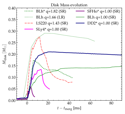
Figure 1.— Time evolution of the total disk mass for a few selected short-lived and long-lived cases. The former show a rapid accretion right after disk formation. The plots show distinct difference in dynamical evolution after disk formation: accretion onto the newly formed BH (short-lived remnants) or accretion onto the NS remnant (DD2 $q=1$) with possible continuous mass shedding from the remnant into the disk (BLh* $q=1$).

Among the comparable-mass ($q\lesssim 1.4$) mergers, the merger outcome is either a short-lived or a long-lived NS remnant. The former collapses to BH within few dynamical periods set by the NS remnant’s rotation, the latter does not collapse within the simulated time. In practice, the short-lived remnants of LS220 $q=1,1.1,1.2$, SFHo $q=1,1.1,1.4$ and SLy $q=1,1.1,1.4$ collapse within $20$ ms postmerger. The exact time of the collapse is strongly dependent on the simulated physics and also on numerical errors. For example, the inclusion turbulent viscosity (Radice, 2017) or changes in the resolution can accelerate or delay the collapse.

The remnant disk originates from the matter expelled by tidal torques and shocks produced at the collisional interface of the NS cores during merger. Starting at merger, the NS remnant sheds mass and angular momentum outwards through spiral density waves streaming from the shock interface (Bernuzzi et al., 2016; Radice et al., 2018a). The maximum temperatures are experienced in these streams that however rapidly decrease because of the expansion and neutrino emission. The electron fraction is reset by an initial excess of electron antineutrino emission and electron neutrino absorption, while the entropy per baryon varies between $3$ and $\lesssim 10\,$$k_{B}$/baryon (Perego et al., 2019). In the short-lived cases, the process quickly shuts down at BH formation: the disk rapidly accretes at early times around the newly formed BH and then reaches a steady state, Fig. 1. The resulting configuration is approximately axisymmetric and Keplerian; it is characterized by neutron-rich $Y_{e}\sim 0.1$ and hot $T\sim 10\,$MeV material in the inner part ($\rho\sim 10^{13}$ ${\mathrm{g}\,cm^{-3}}$) and colder and reprocessed material near the edge $Y_{e}\sim 0.4$. The maximum disk masses (at formation) are generically larger for stiffer EOS and higher mass ratio. The disk mass can be described within the numerical uncertainties by a quadratic function of the mass ratio and the reduced tidal parameters (see Sec. 7). In particular, the most massive disks are formed in case of highly asymmetric BLh $q=1.82$ binary and of the softer EOS LS220 but less asymmetric $q=1.43$ binary. In the latter case the quick collapse of the remnant removes more then half of the disk mass within $40$ ms postmerger.

In the long-lived cases, the disk (now defined by the material with $\rho\lesssim 10^{13}$ ${\mathrm{g}\,cm^{-3}}$) is more massive and extended than the disk around BH remnants (Perego et al., 2019). In general, the maximum disk mass is larger for stiffer EOS and higher mass ratio. For example, the DD2 $q=1$ remnant has disk mass ${\sim}0.2\,{\mathrm{M}_{\odot}}$ while the BLh $q=1$ has ${\lesssim}0.15\,{\mathrm{M}_{\odot}}$. The disk of the BLh $q\sim 1.4-1.5$ remnant is up to a factor two more massive than the latter. The long-term disk evolution is determined by its interaction with the central object. On the one hand the gravitational pull and the neutrino cooling causes the material to accrete. On the other hand the spiral density waves continuously feed the disk with centrifugally supported material, and the angular momentum transport caused by the turbulence favors its expansion. Thus, the disk looses its mass by accretion if the central object is a BH, but can either acquire or loose mass if the central object is a NS. The latter cases are visibile in Fig. 1 for the the BLh EOS and the DD2 EOS. In particular, the BLh* $q=1$ postmerger configuration is such that the mass-shedding by the remnant exceeds the mass accretion. This behaviour is believed to be set by a combination of the EOS softness and the treatment of the thermal effects within the BLh EOS. The former implies stronger postmerger remnant oscillations than the DD2 EOS, the latter higher remnant average temperature.

In terms of disk structure, the inclusion of turbulence appears to smoothen the mass distribution of disk properties, such as $Y_{e}$, $s$, $T$, making them slightly broader. However, detailed quantitative study requires more runs at several resolutions to separate finite-grid from subgrid turbulence effects (Bernuzzi et al., 2020; Radice, 2020).

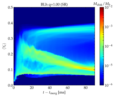
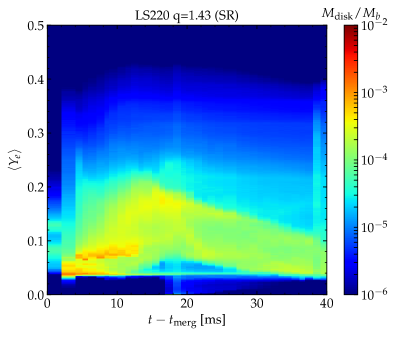
Figure 2.— Evolution of the disk mass-averaged electron fraction with time for a long-lived (top) and a short-lived (bottom) remnant. The plot shows that with time the bulk of the disk lowers its $Y_{e}$ via cooling, while a small fraction in terms of mass gains a high $Y_{e}$, which relates to the highly irradiated surface of the disk.

Disks around long-lived remnant are also more optically thick than disks around BH. The top panel of Figure 2 shows the evolution of the mass-weighted electron fraction for the case of BLh $q=1$ up to $90$ ms. At early times a fraction of fluid elements have $Y_{e}\sim 0.25$ as a results of the shock and spiral waves during formation. After about ${\sim}40$ ms from merger, most of the matter comprises a neutron-rich bulk at $Y_{e}\lesssim 0.1$. Neutrinos irradiate the disk edge (Fig. 10, density contours) that at ${\sim}40$ ms reaches $Y_{e}\sim 0.4$. Note that neutrinos in merger remnants decouple at $\rho\sim 10^{11}$ ${\mathrm{g}\,cm^{-3}}$ (Endrizzi et al., 2020). While we expect this picture to be qualitatively correct, the gap at intermediate $\langle Y_{e}\rangle\simeq 0.15$ might be a artifact of the M0 which assumes radial propagation of neutrinos and cannot correctly capture the reabsorption of neutrinos emitted from the midplane of the disk. In the case of BH remnant (bottom panel of Figure 2), the more compact disk still emits efficiently neutrinos, but due to the lack of emission from the massive NS neutrino absorption at the disk edge is not relevant and the average electron fraction is systematically lower.

If the disk expands outwards sufficiently far, recombination of nucleons into alpha particles provide enough energy to unbind the outermost material and generate mass outflows (Beloborodov, 2008; Lee et al., 2009; Fernández & Metzger, 2013). On the simulated timescales, mass is ejected from the remnant due to the spiral-wave wind (Nedora et al., 2019) and the neutrino-driven wind ($\nu$-component; Dessart et al. 2009; Perego et al. 2014; Just et al. 2015). The former is powered by a hydrodynamical mechanism that preferentially ejects material at low latitudes. The spiral-wave wind can have a mass up to a few $10^{-2}\,{\mathrm{M}_{\odot}}$ and velocities ${\sim}0.2$ c. The ejecta have electron fraction typically larger than ${\sim}0.25$ since they are partially reprocessed by hydrodynamic shocks in the expanding arms. The $\nu$-component is driven by neutrino heating above the remnant. It generates outflows with smaller masses ${\sim}10^{-4}M_{\odot}$ and larger $Y_{e}$ than the spiral-wave wind. Differently from spiral-wave wind the mass flux of the $\nu$-component in our simulations subsides before the end of out simulations, due to rapid baryon loading of the polar region. The spiral-wave wind will be discussed in detail in Sec. 5.

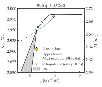
Figure 3.— Baryon mass vs angular momentum diagram for the BLh $q=1$ remnant. The colored diamond marks the baryonic mass and angular momentum at the end of the dynamical gravitational-wave dominated phase. After the GW phase, the evolution is driven by the massive outflows. The solid black line is the $M_{b}$ and $J$ estimated from the 3D data integrals under the assumption of axisymmetry. The green dashed line is a conservative estimate of the mass ejection and a possible trajectory for the viscous evolution as estimated in Radice et al. (2018a). The crosses are a linear extrapolation in time of the solid black line. The gray shaded region is the region of stability of rigidly rotating NS equilibria.

The fate of the long-lived remnant beyond the simulated timescale is difficult to predict without longer, ab-initio simulations in $(3+1)D$ with complete physics. To illustrate this aspect we discuss the representative case of BLh $q=1$ that is one of our longest runs of binaries with baryon mass larger than the one supported by the zero-temperature beta-equilibrated rigidly rotating equilibrium single NS configurations. Figure 3 shows the evolution of the remnant in the baryon mass vs. angular momentum diagram. The total baryon mass of the system is conserved, and in absence of ejecta (e.g.,  during the inspiral) the binary evolves along curves of constant baryonic mass but loses angular momentum due to emission of GWs. The latter is computed from the multipolar GW following Damour et al. (2012); Bernuzzi et al. (2012, 2015), in particular taking the difference between the Arnowitt-Deser-Misner intial angular momentum of the initial data and the angular momentum carried away by the gravitational waves by the end of the simulations. After the GW losses becomes inefficient, the remnant remains to the right with respect to the rigidly rotating equilibria region, marked as the gray shaded area in Fig. 3. This indicate that the remnant has angular momentum in excess with respect to the relative (same baryon mass) NS equilibrium, and it is a generic features of all the simulated binaries (Zappa et al., 2018; Radice et al., 2018a). Additionally, the baryon mass of the remnant after the GW-driven phase is larger than the maximum baryon mass for rigidly rotating equilibria. This is usually called a hypermassive NS remnant, according to a classification based on zero-temperature EOS equilibria (Baumgarte et al., 2000), and it is thus expected to collapse to BH at finite time. After the dynamical GW-dominated phase (yellow diamond) we compute the angular momentum and mass evolution under the assumption of axisymmetry (black solid curve) . Massive ejecta beyond the simulated time can drive the remnant evolution to the stability limit, in contrast with the naive expectation of BH collapse. Indeed, both the extrapolation of the data at longer timescales (black crosses) and a conservative upper bound estimate (Radice et al., 2018a) (green dashed line) are compatible with a possible massive NS remnant close to the Keplerian limit. A linear extrapolation of the final trend indicates that if about $\approx 0.05\,{\mathrm{M}_{\odot}}$ ($\approx 40$% of the disk mass at the final evolution time) of the disk evaporates at the same rate, then the remnant would be close to mass-shedding limit of rigidly rotating equilibria at about ${\sim 300}$ ms postmerger. Note this simulations is with viscosity, but magnetic stresses could further boost ejecta (Metzger et al., 2007; Bucciantini et al., 2012; Siegel & Metzger, 2017; Fernández et al., 2019; Ciolfi, 2020).

A similar outcome is obtained for other binaries. In case of DD2, however, remnants lay below the cusp of the equilibria region, having an excess of angular momentum but not of baryonic mass. The evolution towards the stability is slower in these cases. More asymmetric models are formed with larger excess in the total angular momentum and must shed a larger amount of mass to reach the equilibrium. We estimate that the amount of ejected mass required to reach stability lies between ${\sim}0.05M_{\odot}$ and $0.2M_{\odot}$ for the $q=1$ and $q=1.4$ binaries respectively, again corresponding to $\lesssim 40\%$ of the disk mass.

4. Dynamical Ejecta

The mechanisms behind dynamical ejecta and results for our simulations have been extensively discussed in recent papers (Radice et al., 2018b; Bernuzzi et al., 2020). Here, we focus on the overall properties of the mass ejecta of our set of targeted simulations and provide approximate fitting formulae for the average mass, velocity and electron fraction. Then, we discuss on the applicability of these results for the kN AT2017gfo, associated with the gravitational wave event GW170817.

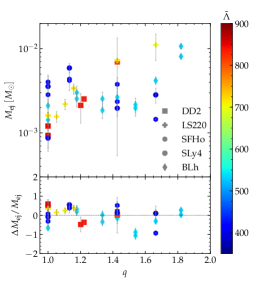
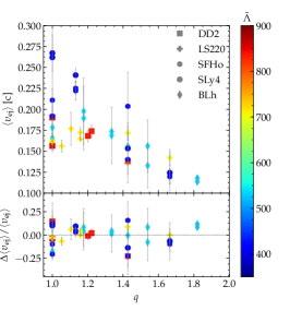
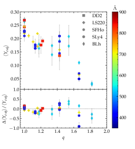
Figure 4.— Dynamical ejecta properties as a function of mass ratio and reduced tidal parameter. The dependency on the latter is color coded. From left to right the main panels show the total mass, the mass-averaged velocity and the electron fraction. The bottom panels show the relative difference between the data and the fit polynomial fit discussed in the text.

The data presented in this work is obtained with the M0 and GRLES schemes and span a significant range in mass ratio but a smaller range in the reduced tidal parameter $\tilde{\Lambda}$ than our previous dataset of Radice et al. (2018b), where most of the simulations were performed with the leakage scheme only. Comparing the data obtained with leakage and those with the M0, we observe that neutrino absorption leads to not only an increased average electron fraction but also to larger total ejected mass and velocity. For example, the mass averaged over the simulations from Tab. 1 is $\overline{M^{\mathrm{d}}_{\mathrm{e}j}}=(3.442\pm 2.495)\times 10^{-3}\,M_{\odot}$ (where hereafter we report also the standard deviation), while the same quantity calculated for data of Radice et al. (2018b) is $\overline{M^{\mathrm{d}}_{\mathrm{e}j}}=(1.352\pm 1.250)\times 10^{-3}\,{\mathrm{M}_{\odot}}$. The mass-averaged terminal velocity of the dynamical ejecta ranges between $0.1$c and $0.3$c, in a good agreement with Radice et al. (2018b). The mass-averaged velocity, averaged over all the simulations, is $\overline{\langle v^{\mathrm{d}}_{\infty}\rangle}=(0.172\pm 0.038)\,{\mathrm{c}}$. The new data at fixed chirp mass shows a correlation of $\langle v^{\mathrm{d}}_{\infty}\rangle$ with the tidal parameter $\tilde{\Lambda}$: the lower the $\tilde{\Lambda}$ the higher the velocity. This is a consequence of the fact that dynamical ejecta in comparable-mass mergers is dominated by the shocked component and that the shock velocity is larger the more compact the binary is . On the contrary, for high mass ratios $q\gtrsim 1.5$, the ejecta is dominated by the tidal component and a larger $q$ leads to a smaller $\langle v^{\mathrm{d}}_{\infty}\rangle$. The mass-averaged electron fraction in our simulations varies between $0.1$ and $0.3$ and averaged among the simulations is $\overline{\langle Y^{\mathrm{d}}_{e}\rangle}=0.175\pm 0.063$. The range is broader than what previously reported in Radice et al. (2018b), where the upper limit was $\approx 0.2$ and the lower was $0.1$. The main difference for this result is the use of the M0 scheme, as noted above. The average electron fraction of our models with M0 neutrino transport is very similar to the ones obtained with M1 scheme of Sekiguchi et al. (2016) and Vincent et al. (2020). Moreover, the high-$q$ simulations where the dynamical ejecta is dominated by the tidal component contribute to the lower boundary of $\langle Y^{\mathrm{d}}_{e}\rangle$. The comparison between simulations with and without the GRLES scheme does not indicate a strong effect on the dynamical ejecta; the effect is comparable to the effect of finite grid resolution, (Bernuzzi et al., 2020; Radice, 2020).

Table 2Coefficients for the polynomial regression with Eq. (10) of the data with chirp mass $\mathcal{M}_{c}=1.188{\mathrm{M}_{\odot}}$ in this paper. The last rows reports coefficient of determination $R^{2}$ of the fit.

	$M^{\mathrm{d}}_{\mathrm{e}j}$ $[10^{3}{\mathrm{M}_{\odot}}]$	$\langle v^{\mathrm{d}}_{\infty}\rangle$ $[c]$	$\langle Y^{\mathrm{d}}_{e}\rangle$	$M_{\mathrm{d}isk}$ $[{\mathrm{M}_{\odot}}]$
$b_{0}$	$54.247$	$0.677$	$-6.607\times 10^{-2}$	$-1.752$
$b_{1}$	$-57.32$	$-0.182$	$0.318$	$2.272$
$b_{2}$	$-6.887\times 10^{-2}$	$-1.083\times 10^{-3}$	$6.084\times 10^{-4}$	$1.139\times 10^{-3}$
$b_{3}$	$13.604$	$-4.912\times 10^{-2}$	$-0.155$	$-0.730$
$b_{4}$	$4.831\times 10^{-2}$	$3.893\times 10^{-4}$	$-2.055\times 10^{-4}$	$-2.921\times 10^{-4}$
$b_{5}$	$1.067\times 10^{-5}$	$4.239\times 10^{-7}$	$-2.896\times 10^{-7}$	$-5.532\times 10^{-7}$
$R^{2}$	$0.716$	$0.779$	$0.769$	$0.498$

Overall, we find that the properties of the ejecta depend strongly on mass-ratio and the EOS softness, that can be parameterized by the reduced tidal parameter. Figure 4 shows the dynamical ejecta properties as a function of the mass ratio and (color coded) $\tilde{\Lambda}$. We can fit of our data at fixed chirp mass using a second order polynomial in these two parameters,

$$P_{2}(q,\tilde{\Lambda})=b_{0}+b_{1}q+b_{2}\tilde{\Lambda}+b_{3}q^{2}+b_{4}q\tilde{\Lambda}+b_{5}\tilde{\Lambda}^{2}\ .$$ (10)

Fitting coefficients are reported in Tab. 2 for all the quantities; fit residuals are displayed in the bottom panel of Fig. 4. We have explored several fitting functions, including several proposals in the literature, and find that overall the choice in Eq. (10) is simple and robust; these results will be reported elsewhere.

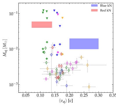
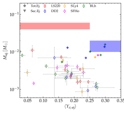
Figure 5.— Summary of the ejecta properties of our models. Diamonds mark the dynamical ejecta, crosses include the contribution of the spiral-wave wind for the long-lived models, triangles are an estimate of the total ejecta mass on a secular timescale, assuming $40\%$ of the disk mass is unbounded on secular timescales. The ejecta mass is shown is terms of the mass-averaged velocity (left) and of the averaged electron fraction (right). The filled blue and red patches are the expected values of ejecta mass and velocity for blue and red components of AT2017gfo compiled by Siegel (2019), based on Villar et al. (2017).

Let us discuss an application of our results to GW170817. We apply the best-fits using the 90% credible intervals estimated of $q$ and $\tilde{\Lambda}$ from the LIGO-Virgo GW analysis (Abbott et al., 2017c, 2019; De et al., 2018; Abbott et al., 2018a), i.e. $\tilde{\Lambda}=300_{-190}^{+500}$ and $q\in[1.,1.37]$. We find $M^{\mathrm{d}}_{\mathrm{e}j}=3.44^{+2.50}_{-2.50}\times 10^{-3}\>M_{\odot}$, $\langle v^{\mathrm{d}}_{\infty}\rangle=0.15^{+0.01}_{-0.15}$c and $\langle Y^{\mathrm{d}}_{e}\rangle\lesssim 0.12$. These values are not compatible with the ejecta properties inferred from AT2017gfo using spherical two-components kN models (Villar et al., 2017). Siegel (2019) estimates that the various fitting models predict $M_{\mathrm{e}j}^{\mathrm{r}ed}\in(4,6)\times 10^{-2}M_{\odot}$ and $\upsilon_{\mathrm{e}j}^{\mathrm{r}ed}\in(0.07,0.14)$ for the red component, while $M_{\mathrm{e}j}^{\mathrm{b}lue}\in(1,2)\times 10^{-2}M_{\odot}$ and $\upsilon_{\mathrm{e}j}^{\mathrm{b}lue}\in(0.2,0.3)$ for the blue component. Thus, neither component can be explained with the dynamical ejecta from our simulations. In Fig. 5 we show the ejecta properties from all our models (diamonds) and the parameters inferred from the observations as red and blue boxes. Despite the fact that $\langle Y^{\mathrm{d}}_{e}\rangle\sim 0.15-0.25$ for comparable masses BNS, none of our models has dynamical ejecta massive enough to account for the red component fit. The NR data also have significantly higher velocities then the one inferred by the two-component kN model. This indicates that additional ejecta components should be considered in order to robustly associate the kN to the ejecta mechanisms (Perego et al., 2017; Kawaguchi et al., 2018; Nedora et al., 2019). The analysis of AT2017gfo with realistic ejecta models and possibly more realistic radiation transfer simulations is beyond the scope of this work, and will be performed in future work. We will refer to Fig. 5 throughout the text when discussing the spiral-wave wind and possible winds from the remnant disks.

5. Spiral-waves wind

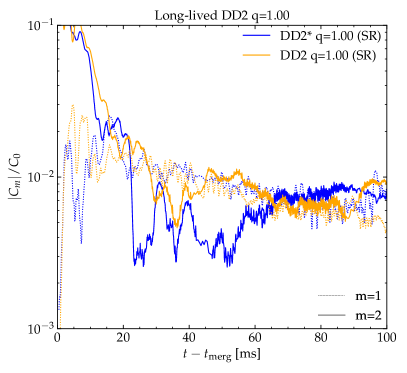
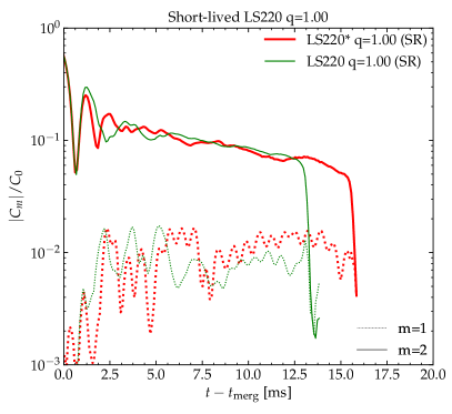
Figure 6.— Modes analysis for exemplary equal-mass long-live and short-lived remnants. The evolution of the $m=2$ and the $m=1$ monitored by Eq. (4) is shown for the DD2 and LS220 remnant with and without turbulent viscosity. The $m=2$ mode in the long-lived remnant is strongly damped by the emission of gravitational radiation and becomes comparable to the $m=1$ mode on a timescale of ${\gtrsim}20\,$ms. Turbulent viscosity sustain the $m=2$ mode for a longer period. The $m=2$ mode is instead dominant to collapse in the short-lived remnant.

In this section we discuss in detail the spiral waves dynamics and the associated spiral-wave wind. We postprocess the simulations to compute the hydrodynamical modes of the NS remnants using the method discussed in Sec. 2.4. The mode analysis for few representative cases is shown in Fig. 6. The remnant NS is strongly deformed with the characteristic spiral arms developing from the cores’ shock interface and expanding outwards (Shibata & Uryu, 2000; Shibata & Taniguchi, 2006; Bernuzzi et al., 2014; Kastaun & Galeazzi, 2015; East et al., 2016b; Paschalidis et al., 2015; Radice et al., 2016a; Lehner et al., 2016b). At early times the main deformation is a $m=2$ bar-shaped mode, while at later times a $m=1$ mode become the dominant deformation (East et al., 2016b; Paschalidis et al., 2015; Radice et al., 2016a; Lehner et al., 2016b; Bernuzzi et al., 2014; Kastaun & Galeazzi, 2015). In the short-lived LS220 $q=1$ binary, the $m=1$ mode is subdominant with respect to the $m=2$, and it reaches a maximum close to the collapse (cf. Bernuzzi et al., 2014). Instead, in the long-lived remnant DD2 $q=1$ the $m=1$ mode becomes at least comparable to the $m=2$ mode at ${\sim}20$ ms and persists throughout the remnant’s lifetime, while the $m=2$ mode efficiently dissipates via GW emission (Bernuzzi et al., 2016; Radice et al., 2016a). With respect to the mass ratio we observe that the magnitude of the $m=1$ mode increases with $q$. In particular, BLh $q=1.43$ and LS220 $q=1.22$ show the largest $C_{m=1}$. Thus remnants from asymmetric binary mergers exhibit stronger $m=1$ modes, which in turn leads to a larger spiral-wave wind mass flux. Regarding $C_{m=2}$, we observer no clear trend in $q$. This is in agreement with what reported by Lehner et al. (2016b).

The spiral arms in a remnant are a hydrodynamics effect that is present also in simulations with polytropic EOS and without weak interactions (Bernuzzi et al., 2014; Radice et al., 2016a). However, the quantitative development of these modes in a remnant is affected by the physics input. For example, Fig. 6 highlights that turbulent viscosity in the DD2 remnant helps sustaining the $m=2$ mode in time, thus boosting angular momentum transport into the disk. By contrast, the $m=1$ modes are not significantly affected by viscosity. On the other hand, viscosity effects are not significant on short timescales after merger, and do not affect the dynamics of the LS220 remnant that collapses to BH at ${\sim}15$ ms.

We compute the angular momentum of the NS remnant and the disk under the assumption of axisymmetry and integrating Eq. (8) using $\rho=10^{13}$ ${\mathrm{g}\,cm^{-3}}$ as a cutting density. We observe that, for all long-lived remnants, ${\sim}50\%$ of the angular momentum available at formation is transported into the disk during the first ${\sim}20$ ms. Henceforth, the disk contains about half of the total angular momentum budget, and the remnant settles on a quasi-stationary evolution track (see Sec. 3). Similarly, we estimate that spiral density modes inject ${\sim}0.1-0.4\,{\mathrm{M}_{\odot}}$ of baryon mass into the disk during the first ${\sim}20$ms. For the same mass and mass ratio $q=1$, the DD2 remnant sheds a larger mass into the disk than the BLh remnant, suggesting that the process might be more efficient for stiffer EOS. Unequal mass binaries form a larger disks than equal mass binaries; compare, for instance, BLh* $q=1.82$ and LS220* $q=1.43$ on the Fig. 1.

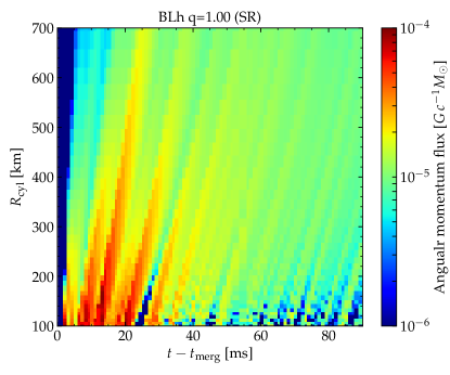
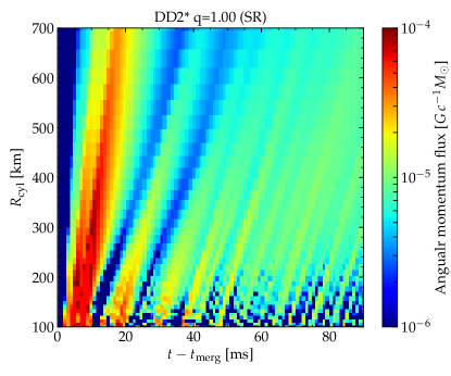
Figure 7.— Angular momentum flux through consecutive cylindrical surfaces identified by cylindrical radii from $R_{\mathrm{c}yl}=100$ to $R_{\mathrm{c}yl}=500$. The plot shows the angular momentum transport into the disk.

The angular momentum transported into the disk is shown in Fig. 7 for the DD2 and BLh $q=1$ remnants. Angular momentum is transported by waves propagating in the disk. These correspond to the spiral density waves in the remnant with $m=1,2$ geometry described above. The angular momentum transported during the first waves is larger for the more massive DD2 disk than for the BLh. DD2* and BLh* show qualitative differences in their evolution starting at ${\sim}20$ ms postmerger. While the DD2* remnant continues to accrete and its disk decreases in mass, the BLh* remnant keeps on shedding more material into the disk than what it accretes. See Fig. 1 and discussion in Sec. 3. The reason is the strong angular momentum flux from the central region in the BLh* case as well as the larger temperature reached in this model, which lowers the rotational frequency at which mass shedding takes place (Kaplan et al., 2014). More simulations of the long-lived remnant evolution are required to investigate the effects of mass-ratio and subgrid turbulence.

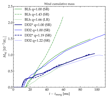
Figure 8.— Cumulative mass of the spiral-wave wind from long-lived remnants. The wind persists on timescales of $\mathcal{O}(100)\,$ ms with mass fluxes ${\sim}0.33-1.23\,{\mathrm{M}_{\odot}}/s$.

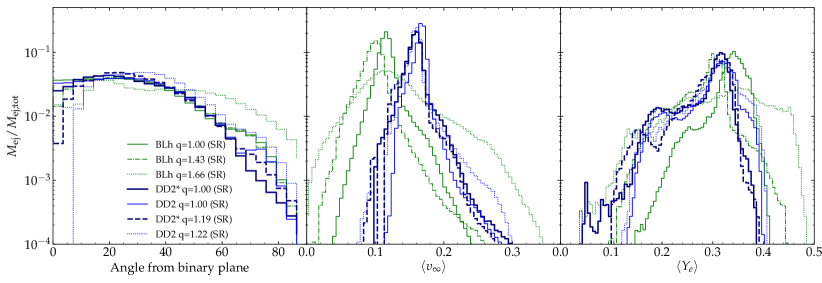
Figure 9.— Mass-averaged histograms of the spiral-wave wind for a selected subset of long-lived remnant. From left to right: ejecta angular distribution, ejecta terminal velocity and electron fraction. Remnants from more asymmetric binaries produce winds with broader angular distribution. The spiral-wave wind from the DD2 EOS remnants has larger velocities then the winds from the softer BLh EOS. The electron fraction peaks at ${\sim}0.3$ and it is distributed from $0.1$ to $0.4$.

Table 3Summary table of the spiral-wave wind properties of long-lived remnants. The columns contain the following information, starting from the left. Equation of state, mass-ratio, available resolutions, inclusion of subgrid turbulence, time of the simulation end, mass of the spiral-wave wind, mass-loss rate via spiral-wave wind, mass-averaged electron fracton, terminal velocity and, finally, RMS angle for spiral-wave wind. For these four quantities we give the mean value among the resolutions and one-sigma deviations. For binaries for which only one resolution is present, the error is assumed to be $20\%$ of the value.

EOS	$q$	Resolution	GRLES	$t_{\text{end}}$	$M^{\mathrm{w}}_{\mathrm{e}j}$	$M^{\mathrm{w}}_{\mathrm{e}j}/\Delta t$	$\langle Y^{\mathrm{}}_{e}\rangle$	$\langle v^{\mathrm{w}}_{\infty}\rangle$	$\langle\theta_{\text{ej}}^{\text{w}}\rangle$
				[ms]	$[10^{-2}M_{\odot}]$	$[M_{\odot}/s]$		$[c]$
BLh	1.18	LR	✓	$69.4$	$1.28^{+0.64}_{-0.64}$	$1.23^{+0.25}_{-0.25}$	$0.33^{+0.01}_{-0.01}$	$0.11^{+0.02}_{-0.02}$	$14.98^{+2.00}_{-2.00}$
BLh	1.43	LR SR	✓	$35.1$ $59.6$	$0.75^{+0.18}_{-0.18}$	$1.06^{+0.67}_{-0.67}$	$0.27^{+0.01}_{-0.01}$	$0.09^{+0.01}_{-0.01}$	$19.43^{+2.22}_{-2.22}$
BLh	1.54	LR	✓	$45.8$	$0.63^{+0.32}_{-0.32}$	$0.44^{+0.09}_{-0.09}$	$0.32^{+0.01}_{-0.01}$	$0.10^{+0.02}_{-0.02}$	$21.46^{+2.00}_{-2.00}$
BLh	1.66	LR SR	✓	$64.6$ $20.1$	$0.12^{+0.09}_{-0.09}$	$0.37^{+0.34}_{-0.34}$	$0.33^{+0.05}_{-0.05}$	$0.13^{+0.01}_{-0.01}$	$52.08^{+20.89}_{-20.89}$
DD2	1.00	LR SR HR	✓	$123.0$ $113.0$ $74.4$	$1.25^{+0.14}_{-0.14}$	$1.30^{+0.19}_{-0.19}$	$0.30^{+0.01}_{-0.01}$	$0.17^{+0.00}_{-0.00}$	$14.88^{+0.87}_{-0.87}$
DD2	1.20	LR SR HR	✗	$37.3$ $91.0$ $55.2$	$0.48^{+0.09}_{-0.09}$	$0.74^{+0.24}_{-0.24}$	$0.26^{+0.01}_{-0.01}$	$0.15^{+0.00}_{-0.00}$	$24.54^{+2.23}_{-2.23}$
DD2	1.43	LR SR	✓	$37.7$ $62.0$	$0.60^{+0.02}_{-0.02}$	$0.51^{+0.06}_{-0.06}$	$0.23^{+0.12}_{-0.12}$	$0.16^{+0.00}_{-0.00}$	$21.74^{+0.03}_{-0.03}$
SFHo	1.43	SR	✓	$46.5$	$0.58^{+0.30}_{-0.30}$	$0.43^{+0.09}_{-0.09}$	$0.31^{+0.01}_{-0.01}$	$0.17^{+0.02}_{-0.02}$	$22.67^{+2.00}_{-2.00}$
SLy4	1.43	SR	✓	$40.3$	$0.53^{+0.27}_{-0.27}$	$0.38^{+0.08}_{-0.08}$	$0.29^{+0.01}_{-0.01}$	$0.18^{+0.02}_{-0.02}$	$23.52^{+2.00}_{-2.00}$

Spiral-density waves in long-lived remnants trigger a massive spiral-wave wind (Nedora et al., 2019). The spiral-wave wind is computed with the Bernoulli criterion described in Sec. 2.4. Summary data are reported in Tab. 3. Figure 8 shows the total wind unbound mass as a function of time. The wind is monitored after the mass flux of the dynamical ejecta (computed according to the geodesic criterion) has saturated. Mass outflows due to the spiral-wave wind continue for all the duration of the simulations with no indication of saturation. Indeed, while mass and angular momentum injection from the high-density core of the remnant into the disk decreases with time as the system becomes more stationary, the mass ejection is expected to continue for as long as the spiral waves persist. Because the $m=1$ modes are not efficiently damped (Paschalidis et al., 2015; Radice et al., 2016a; Lehner et al., 2016b; East et al., 2016a), the ejection can in principle continue for the timescales that the system needs to reach equilibrium or to collapse to BH (Sec. 3).

The largest wind masses are obtained for asymmetric binaries like BLh $q=1.67$ and LS220 $q={\color[rgb]{1,0,0}1.4}$ that in about ${\sim}50$ ms unbind ${\sim}0.02\,{\mathrm{M}_{\odot}}$ with the rate of ${\sim}0.5\,{\mathrm{M}_{\odot}}/{\mathrm{s}}$. We find that models with softer EOS, achieve higher mass flux at lower mass-ratios, i.e., the mass flux of BLh* $q=1.66$ is achieved by LS220* with $q=1.22$. This might be attributed to softer EOS models having a stronger $m=1$ modes in the remnant (see Sec. 7). However, if these remnants collapse, the spiral-wave mechanism shuts down and the outflow terminates. Thus the total ejected mass via spiral-wave wind depends directly on the lifetime of the remnant in addition to the binary parameters, EOS and mass ratio.

Thermal effects play an important role in determining the outflow properties, because high thermal pressures result in more extended disks with material that is more easy to unbind. The highest temperatures in our simulations are found for the BLh EOS. On longer timescales than those simulated, the spiral-wave wind from the remnants with stiffer EOS might be larger, also in relation to the larger disk masses (Sec. 3). Overall, the spiral-wave wind from the long-lived remnant has a mass flux $\geq 0.4\,{\mathrm{M}_{\odot}}/{\mathrm{s}}$.

The property of the spiral-wave wind are found to be remarkably uniform across our simulated sample of remnants. In Fig. 9, we show mass-histograms of the wind angular distribution, velocity and electron fraction. The ejecta mass is distributed around the orbital plane in a large solid angle, similarly to the dynamical ejecta. The electron fraction is broadly distributed in $0.1\lesssim\langle Y^{\mathrm{}}_{e}\rangle\lesssim 0.4$ and peaks around ${\sim}0.35$. Notably, the neutron rich tail of the distribution is determined by the early time spiral-wave wind, before the quasi-steady state outflow sets in. The velocity peaks above ${\sim}0.1\,$c for a softer EOS and around ${\sim}0.2\,$c for a stiffer EOS. If this picture is confirmed by future simulations, this would imply an EOS dependent distinct feature in the electromagnetic counterpart. In particular, the observation of a fast blue kN given by the spiral-wave wind should be associated to a stiff EOS.

Assuming that the source of AT2017gfo was a long-lived remnant surviving for at least $\mathcal{O}(100)$ ms, the spiral-wave wind would significantly contribute the kN. In Fig. 5 we report the total (dynamical+spiral-wave wind) ejecta mass and mass-averaged velocity for the simulated long-lived BNS (crosses). The ejecta mass and electron fraction in BLh $q=1.18,1.42$ and DD2 is $q=1$ are compatible with the blue component inferred using the two-component kN fit (Villar et al., 2017). However, the velocity is significantly lower than that estimated using Villar et al. (2017) models. Note that a multi-component fitting model that explicitly accounts for the spiral-wave wind can fit the early blue emission from AT2017gfo (Nedora et al., 2019). The emission from lanthanide-rich ejecta, however, cannot be explained by the ejecta launched within the first ${\sim}100\,$ms of the remnant evolution. It is thus necessary to consider mass outflows on a longer timescales, as we shall discuss below (Lee et al., 2009; Fernández & Metzger, 2016; Siegel & Metzger, 2017; Fujibayashi et al., 2018; Fernández et al., 2019; Radice et al., 2018a).

6. Neutrino-driven wind

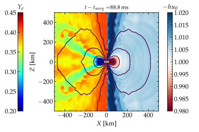
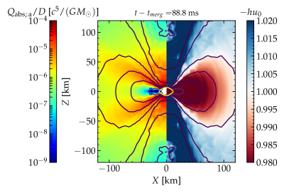
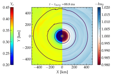
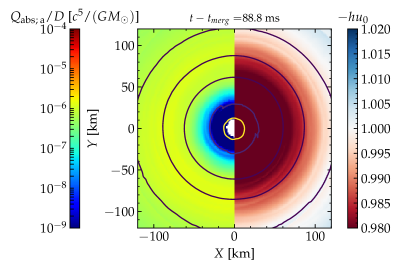
Figure 10.— Snapshot of the $(x,z)$ and $(x,y)$ slices of the BLh $q=1$ model at ${\sim}89\,$ms after merger. Left panels: electron fraction and $-hu_{0}$. High $Y_{e}$ values indicate neutrino postprocessing and irradiation. The $-hu_{0}>1$ indicates the material that gains enough energy to become unbound at infinity. Right: $-hu_{0}$ and the absorption energy rate $Q_{\mathrm{a}bs;\>\bar{\nu}_{e}}$ of electron antineutrinos normalized to the fluid density $D$.

We study in more detail the polar component of the Bernoulli ejecta and suggest that the outflow above the remnant is mostly driven by neutrino absorption rather than by the spiral wave mechanisms. Neutrino interactions above the remnant produce a baryonic outflow that develops parallel to the rotational axis on timescales of ${\sim}\mathcal{O}(10)$ ms postmerger (Perego et al., 2014). Inside this wind, rotational support creates a funnel around the rotational axis as shown in Fig. 10. In the figure we present the electron fraction, the Bernoulli parameter $-hu_{t}$ and the heating energy rate due to electron anti-neutrino absorption $Q_{\mathrm{a}bs;\>\bar{\nu}_{e}}$ divided by with $D=W\rho\sqrt{\gamma}$ ( fluid’s conserved rest-mass density) for the BLh $q=1$ remnant. We consider both the $(x,z)$ and the $(x,y)$ planes, while in the right panels we focus on the innermost part of the remnant. The electron fraction in the polar region with angle from binary plane $\theta>60^{\circ}$ reaches $Y_{e}\sim 0.35$ due to the absorption of electron-type neutrinos. Neutrino heating is maximal close to the bottom of the funnel where the $\nu$-component originates. This corresponds to densities $\rho\sim 10^{11}$ ${\mathrm{g}\,cm^{-3}}$, in the vicinity of neutrino decoupling region (Endrizzi et al., 2020). Large magnetic fields can further boost and stabilize the collimated outflow in the polar region (Bucciantini et al., 2012; Ciolfi, 2020; Mösta et al., 2020).

We confirm that the high latitude outflows constitute a $\nu$-component by studying the correlation between the Bernoulli parameter $-hu_{t}$ and $E_{\nu}/D$. Moreover, we verified that simulations without neutrino heating (i.e. employed only a leakage scheme) do not have this mass ejecta in the polar region. A robust distinction between the $\nu$-component and the spiral-wave wind is impossible to draw at intermediate latitudes ($\theta\sim 45^{\circ}$), where both mechanisms are at work. The mass of the $\nu$-component can be estimated either taking the ejected material with $\theta>60^{\circ}$ or selecting $Y_{e}>0.35$. Contrary to the main component of the spiral-wave wind we find that, for both criteria, the mass flux of $\nu$-component is time-dependent, exhibiting strong growth after merger with a rapid decay in time. For most models, by the end of the run, the mass flux saturates, resulting in a total of ${\sim}10^{-3}-10^{-4}M_{\odot}$ being ejected. We backtrace the cause of this flow interruption to the presence of high density material that is lifted by thermal pressure from the disk and pollutes the polar regions. The properties of this outflow are qualitatively similar to the ones discussed in e.g. Dessart et al. (2009); Perego et al. (2014); Fujibayashi et al. (2020b). In some of these models the $\nu$-component develops over longer timescales than those considered here, it achieves a quasi-steady state and it possibly unbinds larger masses. These differences could result from the conservative choices we have done in isolating the $\nu$-component contribution and in the lack of spiral-wave wind in the other models. Moreover, it could be that the right conditions for the formation of a steady $\nu$-component might not have been reached in our simulations yet.

7. Remnant disk structure

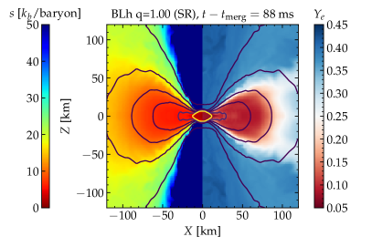
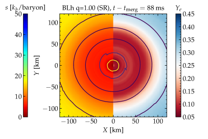
Figure 11.— Entropy and electron fraction on the $(x,z)$ (top) and $(x,y)$ planes (bottom) for the remnant of BL $q=1$ at the end of the simulation. Each plot is divided vertically, with entropy being color-coded on the right and electron fraction on the left. Solid contours stand for rest muss density. Counting from the center, the values are $[10^{13},10^{12},10^{11},10^{10},10^{9}]$ g cm^-3, with the inner most contour encompassing the remnant.

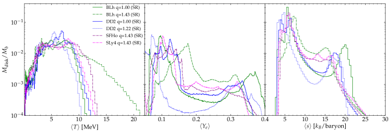
Figure 12.— Composition of the disks at the end of the long-lived remnants simulations. The histograms refer to the temperature $T$ (left), entropy $s$ (middle) and electron fraction $Y_{e}$ (right).

We now discuss the disk structure in long-lived remnants at the end of our simulations, namely at ${\sim}60{-}100$ ms postmerger, and the final disk masses of all our models.

We find that disks around remnant are geometrically thick, with a RMS opening angle of $\langle\theta\rangle_{\mathrm{r}ms}\sim 60^{\circ}$, rather independent of the EOS and $q$. Meanwhile, the radial extend is larger for softer EOS and for larger $q$. The final disk masses range between ${\sim}0.1M_{\odot}$ and ${\sim}0.4M_{\odot}$ (see Tab. 1); smaller masses are obtained for short-lived remnants and for equal-masses binaries. The mean value and standard deviation are $\overline{M}_{\mathrm{d}isk}=(0.161\pm 0.083)M_{\odot}$. Similarly to what we did for the dynamical ejecta, we fit the disk masses with a second order polynomial in $(q,\tilde{\Lambda})$. The coefficients of Eq. (10) for this fit are given in Tab. 2. A more detailed study with various fitting formulas and extended datasets from the literature is reported in a companion paper.

The disk composition at ${\sim}60{-}100$ms postmerger is not uniform, and we study it using the mass-weighted histogram reported in Fig. 12. The entropy and the electron fraction show a bimodal distribution which is more prominent for equal-mass binaries and less prominent for large $q$ ones. The mass-weighted distribution of the entropy shows a dominant peak at low entropy $s\sim 5-10k_{B}/$baryon. This peak is rather EOS and $q$ independent and it correspond to the inner, mildly shocked material. The second, subdominant peak is located at larger entropies, $s\sim 15-22k_{B}/$baryon,and it is more depended on the EOS model: for softer EOSs a larger amount of mass reaches a larger entropy, while for more asymmetric binaries the second peak is centered around lower values of the entropy. Similarly, we observe a first peak in the $Y_{e}$ distribution, around $Y_{e}\sim 0.1$, that corresponds to the neutrino-shielded bulk of the disk. The second (subdominant in mass) peak is at $Y_{e}\sim 0.3-0.4$ and it corresponds to the irradiated disk surface. We stress that, both for the entropy and the electron fraction, the two peaks refer to different regions inside the disk, as visible in Fig. 11. Most of the matter in the disk has temperatures in the range $T\sim 1-10\,$MeV. The inner part of the disk is hotter than the edge. The temperature distribution is also weakly independent of the EOS and mass ratio.

Nuclear recombination is expected to unbind a fraction of the disk mass on secular timescales of a few seconds, longer than those simulated here. Simulations and analytical estimates indicate that up to ${\sim}40\%$ of the disk would become unbound due to viscous processes, with typical velocities of the order of ${\lesssim}0.1\,$c (Lee et al., 2009; Fernández & Metzger, 2016; Wu et al., 2016; Siegel & Metzger, 2017; Fujibayashi et al., 2018; Fernández et al., 2019; Radice et al., 2018a; Fujibayashi et al., 2020b). Assuming these values, the mass of the secular wind from our simulated remnant disks would amount to ${\sim}0.05\,M_{\odot}$. We include this secular wind estimate in Fig. 5 for the long-lived remnants (lower triangles). The estimated mass is sufficient to explain the red component of AT2017gfo, as inferred from the two-components kN models of Villar et al. (2017).

8. Nucleosynthesis

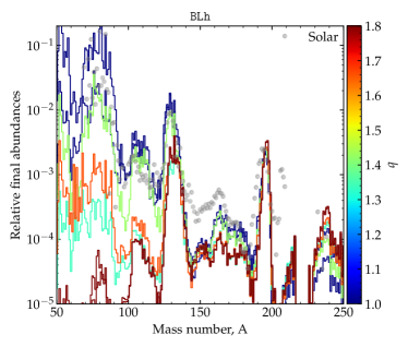
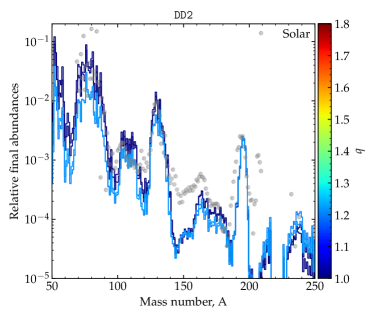
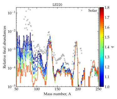
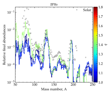
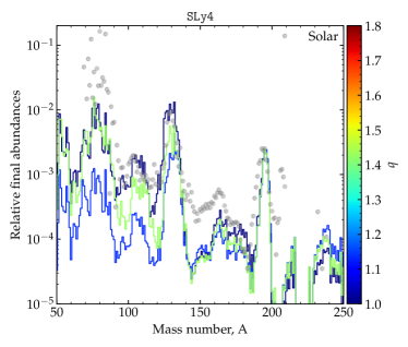
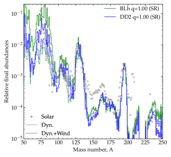
Figure 13.— Nucleosynthesis yields for all simulations. Each of the first five panels shows a different EOS and the scale color the dependency on the mass ratio. The nucleosynthesis is computed on the total ejecta computed during the simulations and composed of the dynamical (all models) plus the spiral-wave wind (for the long-lived remnants listed in Tab. 3.). The last (bottom-right) panel compares the nucleosynthesis in the dynamical ejecta and spiral-wave wind for the long-lived remnants. The inclusion of the spiral-wave wind contributes to improve the agreement with solar data for elements around the first peak.

The nucleosynthesis calculations are performed in postprocessing following the same approach as in Radice et al. (2016b, 2018b). We report the abundances as a function of the mass number $A$ of the different isotopes synthesized by the $r$-process 32 years after the merger in the material ejected from the system. Comparing to our previous study (Radice et al., 2018b), the new simulations allow us to investigate more in detail the nucleosynthesis in presence of neutrino absorption, the contribution of the spiral-wave wind in long-lived remnant, and the effect of mass ratio up to $q\sim 1.8$.

Figure 13 shows the nucleosynthesis yields from the dynamical ejecta (short-lived remnants) and from the dynamical ejecta + wind (long-lived remnants). We compare the abundances inferred from the simulations with up-to-date solar residual $r$-process abundances from Prantzos et al. (2020) (for a review of the solar system abundances see e.g., Pritychenko 2019). To compare the different distributions, we shift the abundances from our models such that they are always the same as the solar one for $A=195$. Notably, all the $r$-process peaks are reproduced by the nucleosynthesis in the ejecta expelled by the long-lived DD2 and BLh models. This demonstrates that the complete solar $r$-process abundances can be recovered if the remnant is long-lived and shows the presence of a spiral-wave wind. This is a consequence of the robust properties of the latter. The possibility of short-lived binaries to reproduce the solar $1$st and $2$nd r-process peaks, at $A\sim 75$ and $A\sim 125$ respectively, strongly depends on the mass-ratio. Higher-$q$ binaries, whose dynamical ejecta is mostly of tidal tail origin with very low electron fraction, show severe underproduction of light $r$-process material. On the contrary, $q\sim 1$ binaries reproduce both peaks reasonably well. This is the result of inclusion of neutrino reabsorption as it increases the $Y_{e}$ of the shocked component of the ejecta (Radice et al., 2018b).

We find that actinides ($A\sim 230$) are produced in all our models, but their abundances depend sensitively on the mass ratio. Very asymmetric binaries produce larger amounts of low-$Y_{e}$ ejecta which result in an increased production of actinides, broadly compatible with the solar pattern. Interestingly, only the highest mass ratio binaries are able to produce at the same time aboundances close to solar for the $3$rd r-process peak and for actinides around ²³²Th. This suggests that asymmetric mergers (or, alternatively, BHNS mergers), might play an important role for the production of the heaviest elements through $r$-process nucleosynthesis.

For long-lived binaries the dynamical ejecta amounts only to a small fraction of the total mass of material leaving the system, while the spiral-wave wind is the more massive ejecta in our simulations. In the bottom-right panel of Fig. 13 we show how the inclusion of the spiral-wave wind changes the abundances of two representative models. Due to its overall high electron fraction, the spiral-wave wind (see Fig. 9) primarily produces first-peak r-process elements $A<95$. Since the abundances are normalized to the $3$rd peak, the relevant differences are those in the $1$st and $2$nd peaks. We observe that due to the slightly higher average electron fraction of the BLh outflows (Fig. 9), it produces more light elements, $A\sim 75$, then DD2 binary. Both binaries, however, display abundance pattern noticeably close to solar.

In addition to the dynamical ejecta and spiral-wave wind, the $r$-process nucleosynthesis occurs in the neutrino-driven wind and the secular wind from the disk. In the neutrino-driven winds, neutrino irradiation of the expanding ejecta considerably increases the electron fraction. If the velocity of the ejecta is sufficiently low, the material reaches the weak equilibrium with neutrinos in optically thin conditions, and $Y_{e}\leq 0.45$ (Qian & Woosley, 1996). This will further boost weak $r$-process nucleosynthesis of light elements $A<130$ (Dessart et al., 2009; Perego et al., 2014; Just et al., 2015; Martin et al., 2015; Foucart et al., 2016). The viscous- and recombination-driven wind is expected to constitute the bulk of the disk outflow, but this takes place on longer timescales than those considered here. Simulations of such systems (Fernández & Metzger, 2013; Just et al., 2015; Wu et al., 2016; Siegel & Metzger, 2017; Fujibayashi et al., 2018; Fernández et al., 2019) suggest that this component of the outflow will have a broad range of $Y_{e}$ and will synthesize both light and heavy $r$-process nuclei. However, heavy $r$-process production might be suppressed in the case of long-lived massive NS remnants (Metzger & Fernández, 2014; Lippuner et al., 2017).

9. Conclusion

In this work we discussed the long-term postmerger dynamics of $37$ binaries with chirp mass $\mathcal{M}_{c}=1.188\,{\mathrm{M}_{\odot}}$ compatible to the source of GW170817, gravitational mass spanning the range $M\in[2.73,2.88]\,{\mathrm{M}_{\odot}}$ and mass ratio values $q\in[1,1.8]$. Our models were computed with five microphysical EOS compatible with nuclear and astrophysical constraints. Each binary was simulated at multiple resolutions for a total of $76$ simulations. Several simulations were pushed to ${\sim}100$ ms postmerger. Together with our previous data (Bernuzzi et al., 2016; Radice et al., 2016b, 2017, 2018c, 2018a, 2018b; Perego et al., 2019; Endrizzi et al., 2020; Bernuzzi et al., 2020) these simulations form the largest sample of merger simulations with microphysics available to date.

The outcome of the merger was found to be very sensitive to the assumed EOS and to the mass ratio (Radice et al., 2020; Bernuzzi, 2020; Bernuzzi et al., 2020). Soft EOSs and/or large mass ratios result in short lived remnants or prompt collapse to BH. Stiffer EOSs and mass ratio closer to one result in longer lived, possibly stable remnants. In agreement with our previous findings, our new simulations also show that the life time of the remnants and the accretion disk masses are strongly correlated for comparable mass binaries (Radice et al., 2018c, b). Large mass ratio binaries ($q\gtrsim 1.4$) have larger accretion disks than comparable mass binaries and produce massive accretion disks and tidal ejecta even when prompt BH formation occurs (see also Bernuzzi et al., 2020).

The material in the disks can reach high temperatures, $O(10\,{\mathrm{M}eV})$, especially for comparable mass ratio mergers, in which the disk material is predominantly originating at the collisional interface between the NSs. Due to the high-temperatures, the disk material is initially reprocessed to intermediate values of the electron fraction $Y_{e}\simeq 0.25$. However, the disks tend to evolve to a lower $Y_{e}$ of about $0.1$, as expected from the theory of neutrino dominated accretion flows (Beloborodov, 2008; Siegel & Metzger, 2018).

Over long timescales, the evolution of these remnants is the result of a complicated interplay between matter accretion, driven by viscous stresses and neutrino cooling, and matter ejection, driven by neutrino reabsorption and hydrodynamical torques (spiral waves; Radice et al., 2018a). Our results indicate that mass ejection due to winds can be sufficiently efficient to prevent the collapse of remnants that have initial masses above the limit supported by uniform rotation, the so-called hypermassive NSs. The determination of the ultimate fate of binaries with masses that are intermediate between prompt collapse and the maximum mass of nonrotating NSs will necessarily require long-term 3D neutrino-radiation GRMHD simulations.

We studied the dynamical ejection of matter during the mergers as a function of the EOS and mass ratio. The main differences with respect to our previous systematic study (Radice et al., 2018b) are that 1) the new simulations are targeted to GW170817, so they span a smaller range of total masses; 2) the new simulations were all performed with the M0 scheme for approximate neutrino transport; 3) our new simulations cover a much broader range of mass ratios. We find that the inclusion of neutrino reabsorption systematically increases the ejecta mass, as anticipated in (Sekiguchi et al., 2015; Radice et al., 2018b). The ejecta composition in our simulations is compatible with that of Sekiguchi et al. (2016) and Vincent et al. (2020) who use very different approximation schemes for neutrinos. This suggests that modern NR simulations are able to capture at least the leading order neutrino effects reliably. We find that as the mass ratio is increased, the dynamical ejecta mass increases, while velocity, and $Y_{e}$ decrease, although the trend on the ejecta mass is not statistically significant, given the large inferred numerical uncertainties. This suggests kN observations could in principle be used to constrain the binary NS mass ratio. Fits to ejecta and disk masses as a function of the mass ratio and the tidal parameter $\tilde{\Lambda}$ are discussed in a companion paper (Nedora et al. in prep).

If the remnant does not collapse to a BH, the dominant outflow component is found to be the spiral-wave wind (Nedora et al., 2019). This is an outflow driven by spiral density waves that are launched in the disk by the remnant NS as it undergoes the bar-mode and one-armed instabilities (Shibata & Uryu, 2000; Paschalidis et al., 2015; Radice et al., 2016a). The spiral-wave wind generates outflows with a rate ${\sim}0.1{-}0.5\,{\mathrm{M}_{\odot}}\,{\mathrm{s}}^{-1}$ which persist for as long as the remnant does not collapse and until the end of our simulations (up to ${\sim}100$ ms). The ejecta have a narrow distribution in velocities with $\langle v_{\infty}\rangle\simeq 0.2\,c$ and a broad distribution in $Y_{e}$.

At high latitudes, we observed the emergence of a $\nu$-component from the remnants. This high-$Y_{e}$ outflow component has characteristics that are initially similar to those of the $\nu$-winds reported by, e.g., Dessart et al. (2009); Perego et al. (2014); Fujibayashi et al. (2020b). However, in our simulations the $\nu$-component is quickly chocked due to the presence of high density material that is lifted by thermal pressure from the disk and pollutes the polar regions. On the other hand, we remark that previous studies found the emergence of the $\nu$-component only at later times, suggesting that the right conditions for the formation of a steady $\nu$-component might not have been reached in our simulations yet. At the same time, we cannot exclude that the lack of $\nu$-component arises due to a deficiency in our approximate neutrino treatment. The emergence of the $\nu$-component should be revisited once better neutrino transport schemes are available.

We performed nucleosynthesis calculations to analyze the $r$-process yields in the dynamical ejecta and the spiral-wave wind. We find that, because of the strong dependency of $Y_{e}$ on $q$, the yields are sensitive to the binary mass ratio. In particular, very asymmetric binaries produce larger quantities of actinides. Symmetric binaries, instead, tend to produce lighter elements. When the spiral-wave wind is included in the nucleosynthesis calculations, we find that the full solar $r$-process pattern down to $A\simeq 100$ can be reproduced. However, high mass-ratio NSNS mergers (or BHNS mergers) appear to be required to explain the production of actinides.

None of our simulations produce outflows with properties compatible with those inferred from the direct fitting of simple color light curve models to AT2017gfo (Villar et al., 2017). However, anisotropic multi-components kN models informed with our NR data can reproduce some of the key features of AT2017gfo (Perego et al., 2017; Nedora et al., 2019). In particular, the optical emission at 1 day can be explained with a combination of dynamical ejecta and spiral-wave wind from long-lived binaries. However, the rapid collapse of the merger remnant cannot be excluded. For example, Fujibayashi et al. (2020a) found that the kind of high-$Y_{e}$ material needed to explain the optical data from AT2017gfo might also be produced in winds from BH-torus systems. The infrared emission from AT2017gfo can only be explained assuming that ${\sim}20\%$ of the remnant disk are unbind by viscous processes and nuclear recombination on a timescale of a few seconds (e.g., Metzger et al., 2008).

Future work should address the limitations of this study. Self-consistent 3D simulations of NS merger systems forming BHs or massive NSs and spanning even longer timescales up to a few seconds are needed to confirm whether or not AT2017gfo can be explained from first principles. Over these timescales, the use of real neutrino transport schemes, such as grey or spectral M1 (Foucart et al., 2016; Roberts et al., 2016), is imperative, since leakage-based schemes, such as our M0 scheme or the M1-leakage scheme of Sekiguchi et al. (2015); Fujibayashi et al. (2018), cannot correctly treat the diffusion of neutrinos from the interior of the remnant. Finally, the impact of MHD effects in the postmerger still needs to be clarified: they are likely crucial for the launching of jets in NS mergers (Ruiz et al., 2016), but their impact on mass ejection and nucleosynthesis is not as clear (Siegel & Metzger, 2018; Fernández et al., 2019).

References

- Abbott et al. (2017a) Abbott, B. P., et al. 2017a, Astrophys. J., 850, L39, 1710.05836
- Abbott et al. (2017b) ——. 2017b, Phys. Rev. Lett., 119, 141101, 1709.09660
- Abbott et al. (2017c) ——. 2017c, Phys. Rev. Lett., 119, 161101, 1710.05832
- Abbott et al. (2018a) ——. 2018a, Phys. Rev. Lett., 121, 161101, 1805.11581
- Abbott et al. (2018b) ——. 2018b, 1810.02581
- Abbott et al. (2019) ——. 2019, Phys. Rev., X9, 011001, 1805.11579
- Arcavi et al. (2017) Arcavi, I., et al. 2017, Nature, 551, 64, 1710.05843
- Ardevol-Pulpillo et al. (2019) Ardevol-Pulpillo, R., Janka, H. T., Just, O., & Bauswein, A. 2019, Mon. Not. Roy. Astron. Soc., 485, 4754, 1808.00006
- Argast et al. (2004) Argast, D., Samland, M., Thielemann, F., & Qian, Y. 2004, Astron. Astrophys., 416, 997, astro-ph/0309237
- Banerjee et al. (2020) Banerjee, P., Wu, M.-R., & Yuan, Z. 2020, 2007.04442
- Bartos & Marka (2019) Bartos, I., & Marka, S. 2019, Astrophys. J., 881, L4, 1906.07210
- Baumgarte et al. (2000) Baumgarte, T. W., Shapiro, S. L., & Shibata, M. 2000, Astrophys. J., 528, L29, astro-ph/9910565
- Bauswein et al. (2013) Bauswein, A., Goriely, S., & Janka, H.-T. 2013, Astrophys.J., 773, 78, 1302.6530
- Beloborodov (2008) Beloborodov, A. M. 2008, AIP Conf. Proc., 1054, 51, 0810.2690
- Berger & Colella (1989) Berger, M. J., & Colella, P. 1989, Journal of Computational Physics, 82, 64
- Berger & Oliger (1984) Berger, M. J., & Oliger, J. 1984, J.Comput.Phys., 53, 484
- Bernuzzi (2020) Bernuzzi, S. 2020, Invited Review for GERG, 2004.06419
- Bernuzzi et al. (2015) Bernuzzi, S., Dietrich, T., & Nagar, A. 2015, Phys. Rev. Lett., 115, 091101, 1504.01764
- Bernuzzi et al. (2014) Bernuzzi, S., Dietrich, T., Tichy, W., & Brügmann, B. 2014, Phys.Rev., D89, 104021, 1311.4443
- Bernuzzi & Hilditch (2010) Bernuzzi, S., & Hilditch, D. 2010, Phys. Rev., D81, 084003, 0912.2920
- Bernuzzi et al. (2012) Bernuzzi, S., Nagar, A., Thierfelder, M., & Brügmann, B. 2012, Phys.Rev., D86, 044030, 1205.3403
- Bernuzzi et al. (2016) Bernuzzi, S., Radice, D., Ott, C. D., Roberts, L. F., Moesta, P., & Galeazzi, F. 2016, Phys. Rev., D94, 024023, 1512.06397
- Bernuzzi et al. (2020) Bernuzzi, S., et al. 2020, Mon. Not. Roy. Astron. Soc., 2003.06015
- Bombaci & Logoteta (2018) Bombaci, I., & Logoteta, D. 2018, Astron. Astrophys., 609, A128, 1805.11846
- Bonetti et al. (2018) Bonetti, M., Perego, A., Capelo, P. R., Dotti, M., & Miller, M. C. 2018, Publ. Astron. Soc. Austral., 35, 17, 1801.03506
- Bonetti et al. (2019) Bonetti, M., Perego, A., Dotti, M., & Cescutti, G. 2019, Mon. Not. Roy. Astron. Soc., 490, 296, 1905.12016
- Bovard et al. (2017) Bovard, L., Martin, D., Guercilena, F., Arcones, A., Rezzolla, L., & Korobkin, O. 2017, Phys. Rev., D96, 124005, 1709.09630
- Bramante & Linden (2016) Bramante, J., & Linden, T. 2016, Astrophys. J., 826, 57, 1601.06784
- Bucciantini et al. (2012) Bucciantini, N., Metzger, B., Thompson, T., & Quataert, E. 2012, Mon. Not. Roy. Astron. Soc., 419, 1537, 1106.4668
- Chornock et al. (2017) Chornock, R., et al. 2017, Astrophys. J., 848, L19, 1710.05454
- Ciolfi (2020) Ciolfi, R. 2020, 2001.10241
- Coulter et al. (2017) Coulter, D. A., et al. 2017, Science, 1710.05452, [Science358,1556(2017)]
- Cowperthwaite et al. (2017) Cowperthwaite, P. S., et al. 2017, Astrophys. J., 848, L17, 1710.05840
- Côté et al. (2019) Côté, B., et al. 2019, Astrophys. J., 875, 106, 1809.03525
- Damour et al. (2012) Damour, T., Nagar, A., Pollney, D., & Reisswig, C. 2012, Phys.Rev.Lett., 108, 131101, 1110.2938
- Danielewicz et al. (2002) Danielewicz, P., Lacey, R., & Lynch, W. G. 2002, Science, 298, 1592, nucl-th/0208016
- Danielewicz & Lee (2014) Danielewicz, P., & Lee, J. 2014, Nucl. Phys., A922, 1, 1307.4130
- De et al. (2018) De, S., Finstad, D., Lattimer, J. M., Brown, D. A., Berger, E., & Biwer, C. M. 2018, Phys. Rev. Lett., 121, 091102, 1804.08583, [Erratum: Phys. Rev. Lett.121,no.25,259902(2018)]
- Dessart et al. (2009) Dessart, L., Ott, C., Burrows, A., Rosswog, S., & Livne, E. 2009, Astrophys.J., 690, 1681, 0806.4380
- Douchin & Haensel (2001) Douchin, F., & Haensel, P. 2001, Astron. Astrophys., 380, 151, astro-ph/0111092
- Drout et al. (2017) Drout, M. R., et al. 2017, 1710.05443
- Duan et al. (2011) Duan, H., Friedland, A., McLaughlin, G., & Surman, R. 2011, J. Phys. G, 38, 035201, 1012.0532
- East et al. (2016a) East, W. E., Paschalidis, V., & Pretorius, F. 2016a, Class. Quant. Grav., 33, 244004, 1609.00725
- East et al. (2016b) East, W. E., Paschalidis, V., Pretorius, F., & Shapiro, S. L. 2016b, Phys. Rev., D93, 024011, 1511.01093
- Endrizzi et al. (2018) Endrizzi, A., Logoteta, D., Giacomazzo, B., Bombaci, I., Kastaun, W., & Ciolfi, R. 2018, Phys. Rev., D98, 043015, 1806.09832
- Endrizzi et al. (2019) Endrizzi, A. et al. 2019, 1908.04952
- Endrizzi et al. (2020) ——. 2020, Eur.Phys.J.A, 56, 15, 1908.04952
- Evans et al. (2017) Evans, P. A., et al. 2017, 1710.05437
- Fahlman & Fernández (2018) Fahlman, S., & Fernández, R. 2018, Astrophys. J., 869, L3, 1811.08906
- Fernández & Metzger (2013) Fernández, R., & Metzger, B. D. 2013, Astrophys.J., 763, 108, 1209.2712
- Fernández et al. (2015) Fernández, R., Quataert, E., Schwab, J., Kasen, D., & Rosswog, S. 2015, Mon. Not. Roy. Astron. Soc., 449, 390, 1412.5588
- Fernández et al. (2019) Fernández, R., Tchekhovskoy, A., Quataert, E., Foucart, F., & Kasen, D. 2019, Mon. Not. Roy. Astron. Soc., 482, 3373, 1808.00461
- Fernández & Metzger (2013) Fernández, R., & Metzger, B. D. 2013, Mon. Not. Roy. Astron. Soc., 435, 502, 1304.6720
- Fernández & Metzger (2016) ——. 2016, Ann. Rev. Nucl. Part. Sci., 66, 23, 1512.05435
- Foucart et al. (2017) Foucart, F. et al. 2017, Class. Quant. Grav., 34, 044002, 1611.01159
- Foucart et al. (2016) Foucart, F., O’Connor, E., Roberts, L., Kidder, L. E., Pfeiffer, H. P., & Scheel, M. A. 2016, Phys. Rev., D94, 123016, 1607.07450
- Freiburghaus et al. (1999) Freiburghaus, C., Rosswog, S., & Thielemann, F.-K. 1999, Astrophys. J. Letters, 525, L121
- Fujibayashi et al. (2018) Fujibayashi, S., Kiuchi, K., Nishimura, N., Sekiguchi, Y., & Shibata, M. 2018, Astrophys. J., 860, 64, 1711.02093
- Fujibayashi et al. (2017) Fujibayashi, S., Sekiguchi, Y., Kiuchi, K., & Shibata, M. 2017, Astrophys. J., 846, 114, 1703.10191
- Fujibayashi et al. (2020a) Fujibayashi, S., Shibata, M., Wanajo, S., Kiuchi, K., Kyutoku, K., & Sekiguchi, Y. 2020a, Phys. Rev. D, 101, 083029, 2001.04467
- Fujibayashi et al. (2020b) Fujibayashi, S., Wanajo, S., Kiuchi, K., Kyutoku, K., Sekiguchi, Y., & Shibata, M. 2020b, 2007.00474
- Fuller et al. (2017) Fuller, G. M., Kusenko, A., & Takhistov, V. 2017, Phys. Rev. Lett., 119, 061101, 1704.01129
- Galeazzi et al. (2013) Galeazzi, F., Kastaun, W., Rezzolla, L., & Font, J. A. 2013, Phys.Rev., D88, 064009, 1306.4953
- Gizzi et al. (2019) Gizzi, D., O’Connor, E., Rosswog, S., Perego, A., Cabezón, R., & Nativi, L. 2019, Mon. Not. Roy. Astron. Soc., 490, 4211, 1906.11494
- Goodale et al. (2003) Goodale, T., Allen, G., Lanfermann, G., Massó, J., Radke, T., Seidel, E., & Shalf, J. 2003, in Vector and Parallel Processing – VECPAR’2002, 5th International Conference, Lecture Notes in Computer Science (Berlin: Springer)
- Gottlieb & Ketcheson (2009) Gottlieb, S., & Ketcheson, David I.and Shu, C.-W. 2009, Journal of Scientific Computing, 38, 251
- Gourgoulhon et al. (2001) Gourgoulhon, E., Grandclement, P., Taniguchi, K., Marck, J.-A., & Bonazzola, S. 2001, Phys.Rev., D63, 064029, gr-qc/0007028
- Hallinan et al. (2017) Hallinan, G., et al. 2017, 1710.05435
- Hanauske et al. (2017) Hanauske, M., Takami, K., Bovard, L., Rezzolla, L., Font, J. A., Galeazzi, F., & Stöcker, H. 2017, Phys. Rev. D, 96, 043004, 1611.07152
- Hempel et al. (2017) Hempel, M., Oertel, M., Typel, S., & Klähn, T. 2017, JPS Conf. Proc., 14, 010802, 1703.03772
- Hempel & Schaffner-Bielich (2010) Hempel, M., & Schaffner-Bielich, J. 2010, Nucl. Phys., A837, 210, 0911.4073
- Hilditch et al. (2013) Hilditch, D., Bernuzzi, S., Thierfelder, M., Cao, Z., Tichy, W., & Bruegmann, B. 2013, Phys. Rev., D88, 084057, 1212.2901
- Hirai et al. (2015) Hirai, Y., Ishimaru, Y., Saitoh, T. R., Fujii, M. S., Hidaka, J., & Kajino, T. 2015, Astrophys. J., 814, 41, 1509.08934
- Hotokezaka et al. (2018) Hotokezaka, K., Beniamini, P., & Piran, T. 2018, Int. J. Mod. Phys., D27, 1842005, 1801.01141
- Hotokezaka et al. (2013) Hotokezaka, K., Kiuchi, K., Kyutoku, K., Muranushi, T., Sekiguchi, Y.-i., et al. 2013, Phys.Rev., D88, 044026, 1307.5888
- Janiuk (2019) Janiuk, A. 2019, 1907.00809
- Ji et al. (2019) Ji, A. P., Drout, M. R., & Hansen, T. T. 2019, 1905.01814
- Ji et al. (2016) Ji, A. P., Frebel, A., Chiti, A., & Simon, J. D. 2016, Nature, 531, 610, 1512.01558
- Just et al. (2015) Just, O., Bauswein, A., Pulpillo, R. A., Goriely, S., & Janka, H. T. 2015, Mon. Not. Roy. Astron. Soc., 448, 541, 1406.2687
- Kaplan et al. (2014) Kaplan, J., Ott, C., O’Connor, E., Kiuchi, K., Roberts, L., et al. 2014, Astrophys.J., 790, 19, 1306.4034
- Kasen et al. (2013) Kasen, D., Badnell, N. R., & Barnes, J. 2013, Astrophys. J., 774, 25, 1303.5788
- Kasliwal et al. (2017) Kasliwal, M. M., et al. 2017, 1710.05436
- Kastaun et al. (2017) Kastaun, W., Ciolfi, R., Endrizzi, A., & Giacomazzo, B. 2017, Phys. Rev., D96, 043019, 1612.03671
- Kastaun & Galeazzi (2015) Kastaun, W., & Galeazzi, F. 2015, Phys.Rev., D91, 064027, 1411.7975
- Kawaguchi et al. (2018) Kawaguchi, K., Shibata, M., & Tanaka, M. 2018, Astrophys. J., 865, L21, 1806.04088
- Kiuchi et al. (2018) Kiuchi, K., Kyutoku, K., Sekiguchi, Y., & Shibata, M. 2018, Phys. Rev., D97, 124039, 1710.01311
- Korobkin et al. (2012) Korobkin, O., Rosswog, S., Arcones, A., & Winteler, C. 2012, Mon. Not. Roy. Astron. Soc., 426, 1940, 1206.2379
- Korobkin et al. (2020) Korobkin, O., et al. 2020, 2004.00102
- Kulkarni (2005) Kulkarni, S. R. 2005, astro-ph/0510256
- Lattimer & Lim (2013) Lattimer, J. M., & Lim, Y. 2013, Astrophys. J., 771, 51, 1203.4286
- Lattimer & Schramm (1974) Lattimer, J. M., & Schramm, D. N. 1974, Astrophys. J. Letters, 192, L145
- Lattimer & Swesty (1991) Lattimer, J. M., & Swesty, F. D. 1991, Nucl. Phys., A535, 331
- Lee et al. (2009) Lee, W. H., Ramirez-Ruiz, E., & Diego-Lopez-Camara. 2009, Astrophys.J., 699, L93, 0904.3752
- Lehner et al. (2016a) Lehner, L., Liebling, S. L., Palenzuela, C., Caballero, O. L., O’Connor, E., Anderson, M., & Neilsen, D. 2016a, Class. Quant. Grav., 33, 184002, 1603.00501
- Lehner et al. (2016b) Lehner, L., Liebling, S. L., Palenzuela, C., & Motl, P. M. 2016b, Phys. Rev., D94, 043003, 1605.02369
- Li & Paczynski (1998) Li, L.-X., & Paczynski, B. 1998, Astrophys.J., 507, L59, astro-ph/9807272
- Lippuner et al. (2017) Lippuner, J., Fernández, R., Roberts, L. F., Foucart, F., Kasen, D., Metzger, B. D., & Ott, C. D. 2017, Mon. Not. Roy. Astron. Soc., 472, 904, 1703.06216
- Loffler et al. (2012) Loffler, F., et al. 2012, Class. Quant. Grav., 29, 115001, 1111.3344
- Logoteta et al. (2016) Logoteta, D., Bombaci, I., & Kievsky, A. 2016, Phys. Rev., C94, 064001, 1609.00649
- Lyman et al. (2018) Lyman, J. D., et al. 2018, Nat. Astron., 2, 751, 1801.02669
- Machleidt & Entem (2011) Machleidt, R., & Entem, D. R. 2011, Phys. Rept., 503, 1, 1105.2919
- Martin et al. (2015) Martin, D., Perego, A., Arcones, A., Thielemann, F.-K., Korobkin, O., & Rosswog, S. 2015, Astrophys. J., 813, 2, 1506.05048
- Metzger et al. (2010) Metzger, B., Martinez-Pinedo, G., Darbha, S., Quataert, E., Arcones, A., et al. 2010, Mon.Not.Roy.Astron.Soc., 406, 2650, 1001.5029
- Metzger et al. (2008) Metzger, B., Piro, A., & Quataert, E. 2008, Mon.Not.Roy.Astron.Soc., 390, 781, 0805.4415
- Metzger & Fernández (2014) Metzger, B. D., & Fernández, R. 2014, Mon.Not.Roy.Astron.Soc., 441, 3444, 1402.4803
- Metzger et al. (2007) Metzger, B. D., Thompson, T. A., & Quataert, E. 2007, Astrophys. J., 659, 561, astro-ph/0608682
- Metzger et al. (2018) ——. 2018, Astrophys. J., 856, 101, 1801.04286
- Miller et al. (2019) Miller, J. M. et al. 2019, Phys. Rev., D100, 023008, 1905.07477
- Mooley et al. (2018) Mooley, K. P. et al. 2018, Nature, 561, 355, 1806.09693
- Mösta et al. (2020) Mösta, P., Radice, D., Haas, R., Schnetter, E., & Bernuzzi, S. 2020, arXiv:2003.06043, 2003.06043
- Mösta et al. (2018) Mösta, P., Roberts, L. F., Halevi, G., Ott, C. D., Lippuner, J., Haas, R., & Schnetter, E. 2018, Astrophys. J., 864, 171, 1712.09370
- Nedora et al. (2019) Nedora, V., Bernuzzi, S., Radice, D., Perego, A., Endrizzi, A., & Ortiz, N. 2019, Astrophys. J., 886, L30, 1907.04872
- Neilsen et al. (2014) Neilsen, D., Liebling, S. L., Anderson, M., Lehner, L., O’Connor, E., et al. 2014, Phys.Rev., D89, 104029, 1403.3680
- Nicholl et al. (2017) Nicholl, M., et al. 2017, Astrophys. J., 848, L18, 1710.05456
- Nishimura et al. (2017) Nishimura, N., Sawai, H., Takiwaki, T., Yamada, S., & Thielemann, F.-K. 2017, Astrophys. J. Lett., 836, L21, 1611.02280
- Nishimura et al. (2015) Nishimura, N., Takiwaki, T., & Thielemann, F. K. 2015, Astrophys. J., 810, 109, 1501.06567
- O’Connor & Ott (2010) O’Connor, E., & Ott, C. D. 2010, Class. Quant. Grav., 27, 114103, 0912.2393
- Oechslin et al. (2006) Oechslin, R., Janka, H.-T., & Marek, A. 2006, Astron.Astrophys., astro-ph/0611047
- Palenzuela et al. (2015) Palenzuela, C., Liebling, S. L., Neilsen, D., Lehner, L., Caballero, O. L., O’Connor, E., & Anderson, M. 2015, Phys. Rev., D92, 044045, 1505.01607
- Paschalidis et al. (2015) Paschalidis, V., East, W. E., Pretorius, F., & Shapiro, S. L. 2015, Phys. Rev., D92, 121502, 1510.03432
- Perego et al. (2019) Perego, A., Bernuzzi, S., & Radice, D. 2019, Eur. Phys. J., A55, 124, 1903.07898
- Perego et al. (2016) Perego, A., Cabezon, R., & Kaeppeli, R. 2016, Astrophys. J. Suppl., 223, 22, 1511.08519
- Perego et al. (2017) Perego, A., Radice, D., & Bernuzzi, S. 2017, Astrophys. J., 850, L37, 1711.03982
- Perego et al. (2014) Perego, A., Rosswog, S., Cabezon, R., Korobkin, O., Kaeppeli, R., et al. 2014, Mon.Not.Roy.Astron.Soc., 443, 3134, 1405.6730
- Piarulli et al. (2016) Piarulli, M. et al. 2016, Phys. Rev., C94, 054007, 1606.06335
- Pollney et al. (2011) Pollney, D., Reisswig, C., Schnetter, E., Dorband, N., & Diener, P. 2011, Phys. Rev., D83, 044045, 0910.3803
- Prantzos et al. (2020) Prantzos, N., Abia, C., Cristallo, S., Limongi, M., & Chieffi, A. 2020, mnras, 491, 1832, 1911.02545
- Pritychenko (2019) Pritychenko, B. 2019, 1905.06165
- Qian & Woosley (1996) Qian, Y., & Woosley, S. 1996, Astrophys. J., 471, 331, astro-ph/9611094
- Radice (2017) Radice, D. 2017, Astrophys. J., 838, L2, 1703.02046
- Radice (2020) ——. 2020, Special issue Numerical Relativity and Gravitational Waves of Symmetry, arXiv:2005.09002, 2005.09002
- Radice et al. (2017) Radice, D., Bernuzzi, S., Del Pozzo, W., Roberts, L. F., & Ott, C. D. 2017, Astrophys. J., 842, L10, 1612.06429
- Radice et al. (2016a) Radice, D., Bernuzzi, S., & Ott, C. D. 2016a, Phys. Rev., D94, 064011, 1603.05726
- Radice et al. (2020) Radice, D., Bernuzzi, S., & Perego, A. 2020, Ann. Rev. Nucl. Part. Sci., 70, 2002.03863
- Radice et al. (2016b) Radice, D., Galeazzi, F., Lippuner, J., Roberts, L. F., Ott, C. D., & Rezzolla, L. 2016b, Mon. Not. Roy. Astron. Soc., 460, 3255, 1601.02426
- Radice et al. (2018a) Radice, D., Perego, A., Bernuzzi, S., & Zhang, B. 2018a, Mon. Not. Roy. Astron. Soc., 481, 3670, 1803.10865
- Radice et al. (2018b) Radice, D., Perego, A., Hotokezaka, K., Fromm, S. A., Bernuzzi, S., & Roberts, L. F. 2018b, Astrophys. J., 869, 130, 1809.11161
- Radice et al. (2018c) Radice, D., Perego, A., Zappa, F., & Bernuzzi, S. 2018c, Astrophys. J., 852, L29, 1711.03647
- Radice & Rezzolla (2012) Radice, D., & Rezzolla, L. 2012, Astron. Astrophys., 547, A26, 1206.6502
- Radice et al. (2014a) Radice, D., Rezzolla, L., & Galeazzi, F. 2014a, Mon.Not.Roy.Astron.Soc., 437, L46, 1306.6052
- Radice et al. (2014b) ——. 2014b, Class.Quant.Grav., 31, 075012, 1312.5004
- Reisswig et al. (2013a) Reisswig, C., Haas, R., Ott, C. D., Abdikamalov, E., Mösta, P., Pollney, D., & Schnetter, E. 2013a, Phys. Rev., D87, 064023, 1212.1191
- Reisswig et al. (2013b) Reisswig, C., Ott, C., Abdikamalov, E., Haas, R., Mösta, P., et al. 2013b, Phys.Rev.Lett., 111, 151101, 1304.7787
- Roberts et al. (2011) Roberts, L. F., Kasen, D., Lee, W. H., & Ramirez-Ruiz, E. 2011, Astrophys.J., 736, L21, 1104.5504
- Roberts et al. (2016) Roberts, L. F., Ott, C. D., Haas, R., O’Connor, E. P., Diener, P., & Schnetter, E. 2016, 1604.07848
- Rosswog (2005) Rosswog, S. 2005, Astrophys. J., 634, 1202, astro-ph/0508138
- Rosswog & Davies (2003) Rosswog, S., & Davies, M. B. 2003, Mon. Not. Roy. Astron. Soc., 345, 1077, astro-ph/0110180
- Rosswog et al. (2014) Rosswog, S., Korobkin, O., Arcones, A., Thielemann, F. K., & Piran, T. 2014, Mon. Not. Roy. Astron. Soc., 439, 744, 1307.2939
- Rosswog & Liebendoerfer (2003) Rosswog, S., & Liebendoerfer, M. 2003, Mon.Not.Roy.Astron.Soc., 342, 673, astro-ph/0302301
- Rosswog et al. (1999) Rosswog, S., Liebendoerfer, M., Thielemann, F., Davies, M., Benz, W., et al. 1999, Astron.Astrophys., 341, 499, astro-ph/9811367
- Rosswog & Ramirez-Ruiz (2003) Rosswog, S., & Ramirez-Ruiz, E. 2003, Mon.Not.Roy.Astron.Soc., 343, L36, astro-ph/0306172
- Rosswog et al. (2003) Rosswog, S., Ramirez-Ruiz, E., & Davies, M. B. 2003, Mon. Not. Roy. Astron. Soc., 345, 1077, astro-ph/0306418
- Ruan et al. (2018) Ruan, J. J., Nynka, M., Haggard, D., Kalogera, V., & Evans, P. 2018, Astrophys. J., 853, L4, 1712.02809
- Ruffert et al. (1997) Ruffert, M., Janka, H., Takahashi, K., & Schäfer, G. 1997, Astron.Astrophys., 319, 122, astro-ph/9606181
- Ruffert et al. (1996) Ruffert, M. H., Janka, H. T., & Schäfer, G. 1996, Astron. Astrophys., 311, 532, astro-ph/9509006
- Ruiz et al. (2016) Ruiz, M., Lang, R. N., Paschalidis, V., & Shapiro, S. L. 2016, Astrophys. J., 824, L6, 1604.02455
- Safarzadeh & Côté (2017) Safarzadeh, M., & Côté, B. 2017, Mon. Not. Roy. Astron. Soc., 471, 4488, 1707.07691
- Safarzadeh et al. (2019a) Safarzadeh, M., Ramirez-Ruiz, E., Andrews, J. J., Fragos, T., Macias, P., & Scannapieco, E. 2019a, Astrophys. J., 872, 105, 1810.04176
- Safarzadeh et al. (2019b) Safarzadeh, M., Sarmento, R., & Scannapieco, E. 2019b, Astrophys. J., 876, 28, 1812.02779
- Schneider et al. (2017) Schneider, A. S., Roberts, L. F., & Ott, C. D. 2017, Phys. Rev., C96, 065802, 1707.01527
- Schnetter et al. (2004) Schnetter, E., Hawley, S. H., & Hawke, I. 2004, Class.Quant.Grav., 21, 1465, gr-qc/0310042
- Schnetter et al. (2007) Schnetter, E., Ott, C. D., Allen, G., Diener, P., Goodale, T., Radke, T., Seidel, E., & Shalf, J. 2007, 0707.1607
- Sekiguchi (2010) Sekiguchi, Y. 2010, Prog. Theor. Phys., 124, 331, 1009.3320
- Sekiguchi et al. (2011) Sekiguchi, Y., Kiuchi, K., Kyutoku, K., & Shibata, M. 2011, Phys.Rev.Lett., 107, 051102, 1105.2125
- Sekiguchi et al. (2015) ——. 2015, Phys.Rev., D91, 064059, 1502.06660
- Sekiguchi et al. (2016) Sekiguchi, Y., Kiuchi, K., Kyutoku, K., Shibata, M., & Taniguchi, K. 2016, Phys. Rev., D93, 124046, 1603.01918
- Shibata & Taniguchi (2006) Shibata, M., & Taniguchi, K. 2006, Phys.Rev., D73, 064027, astro-ph/0603145
- Shibata et al. (2005) Shibata, M., Taniguchi, K., & Uryu, K. 2005, Phys. Rev., D71, 084021, gr-qc/0503119
- Shibata & Uryu (2000) Shibata, M., & Uryu, K. 2000, Phys. Rev., D61, 064001, gr-qc/9911058
- Siegel (2019) Siegel, D. M. 2019, 1901.09044
- Siegel et al. (2018) Siegel, D. M., Barnes, J., & Metzger, B. D. 2018, 1810.00098
- Siegel & Metzger (2017) Siegel, D. M., & Metzger, B. D. 2017, Phys. Rev. Lett., 119, 231102, 1705.05473
- Siegel & Metzger (2018) ——. 2018, Astrophys. J., 858, 52, 1711.00868
- Skúladóttir, Ása and Hansen, Camilla Juul and Salvadori, Stefania and Choplin, Arthur (2019) Skúladóttir, Ása and Hansen, Camilla Juul and Salvadori, Stefania and Choplin, Arthur. 2019, Astron. Astrophys., 631, A171, 1908.10729
- Smartt et al. (2017) Smartt, S. J., et al. 2017, Nature, 1710.05841
- Soares-Santos et al. (2017) Soares-Santos, M., et al. 2017, Astrophys. J., 848, L16, 1710.05459
- Steiner et al. (2013a) Steiner, A. W., Hempel, M., & Fischer, T. 2013a, Astrophys. J., 774, 17, 1207.2184
- Steiner et al. (2013b) Steiner, A. W., Lattimer, J. M., & Brown, E. F. 2013b, Astrophys. J., 765, L5, 1205.6871
- Symbalisty & Schramm (1982) Symbalisty, E., & Schramm, D. N. 1982, Astrophys. J. Letters, 22, 143
- Tanaka et al. (2017) Tanaka, M., et al. 2017, Publ. Astron. Soc. Jap., 1710.05850
- Tanvir et al. (2017) Tanvir, N. R., et al. 2017, Astrophys. J., 848, L27, 1710.05455
- Troja et al. (2017) Troja, E., et al. 2017, Nature, 1710.05433
- Typel et al. (2010) Typel, S., Ropke, G., Klahn, T., Blaschke, D., & Wolter, H. H. 2010, Phys. Rev., C81, 015803, 0908.2344
- van de Voort et al. (2020) van de Voort, F., Pakmor, R., Grand, R. J., Springel, V., Gómez, F. A., & Marinacci, F. 2020, Mon. Not. Roy. Astron. Soc., 494, 4867, 1907.01557
- van Riper & Lattimer (1981) van Riper, K., & Lattimer, J. 1981, Astrophys. J., 249, 270
- Vassh et al. (2020) Vassh, N., Mumpower, M. R., McLaughlin, G. C., Sprouse, T. M., & Surman, R. 2020, Astrophys. J., 896, 28, 1911.07766
- Villar et al. (2017) Villar, V. A., et al. 2017, Astrophys. J., 851, L21, 1710.11576
- Vincent et al. (2020) Vincent, T., Foucart, F., Duez, M. D., Haas, R., Kidder, L. E., Pfeiffer, H. P., & Scheel, M. A. 2020, Phys. Rev., D101, 044053, 1908.00655
- Wanajo et al. (2014) Wanajo, S., Sekiguchi, Y., Nishimura, N., Kiuchi, K., Kyutoku, K., & Shibata, M. 2014, Astrophys. J., 789, L39, 1402.7317
- Wehmeyer et al. (2019) Wehmeyer, B., Frohlich, C., Côté, B., Pignatari, M., & Thielemann, F.-K. 2019, Mon. Not. Roy. Astron. Soc., 487, 1745, 1908.05617
- Winteler et al. (2012) Winteler, C., Kaeppeli, R., Perego, A., Arcones, A., Vasset, N., Nishimura, N., Liebendoerfer, M., & Thielemann, F.-K. 2012, Astrophys. J. Lett., 750, L22, 1203.0616
- Wu et al. (2016) Wu, M.-R., Fernández, R., Martínez-Pinedo, G., & Metzger, B. D. 2016, Mon. Not. Roy. Astron. Soc., 463, 2323, 1607.05290
- Zappa et al. (2018) Zappa, F., Bernuzzi, S., Radice, D., Perego, A., & Dietrich, T. 2018, Phys. Rev. Lett., 120, 111101, 1712.04267