Time-domain effective-one-body gravitational waveforms
for coalescing compact binaries with nonprecessing spins, tides and self-spin effects

Abstract

We present TEOBResumS, a new effective-one-body (EOB) waveform model for nonprecessing (spin-aligned) and tidally interacting compact binaries. Spin-orbit and spin-spin effects are blended together by making use of the concept of centrifugal EOB radius. The point-mass sector through merger and ringdown is informed by numerical relativity (NR) simulations of binary black holes (BBH) computed with the SpEC and BAM codes. An improved, NR-based phenomenological description of the postmerger waveform is developed. The tidal sector of TEOBResumS describes the dynamics of neutron star binaries up to merger and incorporates a resummed attractive potential motivated by recent advances in the post-Newtonian and gravitational self-force description of relativistic tidal interactions. Equation-of-state dependent self-spin interactions (monopole-quadrupole effects) are incorporated in the model using leading-order post-Newtonian results in a new expression of the centrifugal radius. TEOBResumS is compared to 135 SpEC and 19 BAM BBH waveforms. The maximum unfaithfulness to SpEC data $\bar{F}$ – at design Advanced-LIGO sensitivity and evaluated with total mass $M$ varying between $10M_{\odot}\leq M\leq 200M_{\odot}$ – is always below $2.5\times 10^{-3}$ except for a single outlier that grazes the $7.1\times 10^{-3}$ level. When compared to BAM data, $\bar{F}$ is smaller than $0.01$ except for a single outlier in one of the corners of the NR-covered parameter space, that reaches the $0.052$ level. TEOBResumS is also compatible, up to merger, to high end NR waveforms from binary neutron stars with spin effects and reduced initial eccentricity computed with the BAM and THC codes. The data quality of binary neutron star waveforms is assessed via rigorous convergence tests from multiple resolution runs and takes into account systematic effects estimated by using the two independent high-order NR codes. The model is designed to generate accurate templates for the analysis of LIGO-Virgo data through merger and ringdown. We demonstrate its use by analyzing the publicly available data for GW150914.

I Introduction

Analytical waveform models informed by (or calibrated to) numerical relativity (NR) simulations are essential for the analysis of gravitational wave (GW) events Abbott et al. (2016a, b, 2017a, 2017b). The effective-one-body (EOB) approach to the general relativistic two-body problem Buonanno and Damour (1999, 2000); Damour (2001); Damour et al. (2000) is a powerful analytical tool that reliably describes both the dynamics and gravitational waveform through inspiral, merger and ringdown for BBHs Bohé et al. (2017); Nagar et al. (2017); Cotesta et al. (2018) and up to merger for BNSs Dietrich and Hinderer (2017). The analytical model is crucially improved in the late-inspiral, strong-field, fast-velocity regime by NR information, that allows one to properly represent the merger and ringdown part of the waveform Damour and Nagar (2014a); Bohé et al. (2017); Nagar et al. (2017). The synergy between EOB and NR creates EOBNR models, whose more recent avatars implemented in publicly available LIGO Scientific Collaboration Algorithm Library (LAL) LIGO Scientific Collaboration are SEOBNRv4/SEOBNRv4T Bohé et al. (2017); Cotesta et al. (2018), that describe nonprecessing binaries (both BNSs and BBHs) and SEOBNRv3 Babak et al. (2017), that incorporates precession for BBHs. The purpose of this paper is to introduce TEOBResumS, a state-of-the art EOB model, informed by BBH NR simulations, that is fit to describe the dynamics and waveforms from nonprecessing coalescing binaries, both black holes and neutron stars. For BBH binaries, TEOBResumS is an improvement of the model of Refs. Nagar et al. (2017, 2016); Damour and Nagar (2014b) implementing a refined phenomenological representation of the postmerger waveform (ringdown). The latter is built from an effective fit of many spin-aligned NR waveform data available in the SXS catalog SXS obtained with the SpEC code Buchman et al. (2012); Chu et al. (2009); Hemberger et al. (2013); Scheel et al. (2015); Blackman et al. (2015); Lovelace et al. (2012, 2011, 2015); Mroue et al. (2013); Kumar et al. (2015); Chu et al. (2016) and, notably, also incorporates test-particle results. We show here the performance of the model over the SXS SXS and BAM waveform catalogs (the latter consisting of simulations produced using the BAM code Bruegmann et al. (2008); Husa et al. (2008)), and check its robustness also outside NR-covered regions of the parameter space.

For BNSs, we built on our previous efforts Bernuzzi et al. (2015a) (see also Kiuchi et al. (2017); Kawaguchi et al. (2018)) and merged together into a single EOB code, tidal and spin effects, so as to produce a complete waveform model of spinning BNSs. We show that the EOB waveform is accurate up to BNS merger by comparing with state-of-the art, high end, NR simulations. The tidal-and-spin model uses most of the existing analytical knowledge. In particular, we incorporate in the EOB model equation-of-state (EOS) dependent self-spin effects at leading-order (also known as spin-induced quadrupole moment or monopole-quadrupole couplings Poisson (1998)). TEOBResumS has been the first EOB model to have these effects. As such, it was used for validating the phenomenological waveform model, PhenomPv2_NRTidal, that incorporates similar self-spin effects Dietrich et al. (2018a) and that was recently used for a detailed study of the parameters of GW170817 Abbott et al. (2018a, b). However, while TEOBResumS was under internal LVC review, leading-order self-spin effects were also included in SEOBNRv4T, though in a different fashion for what concerns the Hamiltonian Bohé et al. (2017); Hinderer et al. (2016); Steinhoff et al. (2016); Vines and Marsat (2018). A targeted comparison between the two models for BNS configurations is described in Sec. VI.

This paper is organized as follows: in Sec. II we remind the reader the main theoretical features of the EOB model for BBHs, compare its performance against the SXS SXS and BAM NR data, test its robustness over a large portion of the parameter space; in Sec. III we discuss the BNS case, focusing on our analytical strategy to incorporate in a consistent, and resummed, way both tidal and spin effects, including the self-spin ones. In this respect, Sec. IV compares the EOB description with the corresponding nonresummed PN-based expressions. Section VI collects selected comparisons (photon potential and, notably, faithfulness) between TEOBResumS, SEOBNRv4 and SEOBNRv4T. To probe our model, that is implemented as publicly available C codes (see Appendix E), for production runs, we also present, in Sec. V, a case study done on the GW150914 event Abbott et al. (2016a). Conclusions are in Sec. VII. The paper is complemented by several technical appendices. Among these, the case of mixed black-hole and neutron-star binaries is discussed in Appendix B.

We use units with $G=c=1$. In the following, the gravitational mass of the binary is $M=M_{A}+M_{B}$, with the two bodies labeled as $(A,B)$. We adopt the convention that that $M_{A}\geq M_{B}$, so as to define the mass ratio $q\equiv M_{A}/M_{B}\geq 1$, the reduced mass $\mu\equiv M_{A}M_{B}/M$, and the symmetric mass ratio $\nu\equiv\mu/M$, that ranges from $0$ (test-particle limit) to $\nu=1/4$ (equal-mass case). The dimensionless spins are addressed as $\chi_{A,B}=S_{A,B}/M_{A,B}^{2}$. We also define the quantities $X_{A}=M_{A}/M$ and $X_{AB}\equiv X_{A}-X_{B}=\sqrt{1-4\nu}$ (with $X_{A}\geq X_{B}$). As convenient spin variables we shall also use $\tilde{a}_{A,B}\equiv X_{A,B}\chi_{A,B}=S_{A,B}/(M_{A,B}M)$.

II Binary Black Holes

General relativity predicts that the GW signal from quasi-circular inspiral-merger of BBHs is chirp-like Maggiore (2007). The GW phase evolution at Newtonian order, i.e. at large separations and low orbital frequencies, is driven by the value of the chirp mass, ${\cal M}_{c}=(M_{A}M_{B})^{3/5}/(M_{A}+M_{B})^{1/5}$. Higher post-Newtonian (PN) corrections depend on the symmetric mass ratio $\nu$ as well as spin-orbit and spin-spin couplings. The analytic description of the dynamics and waveform for coalescing binaries is based on PN theory Damour et al. (2016); Bernard et al. (2018); Blanchet (2014). However, PN results, an expansion in the small parameter $(v/c)^{2}$, where $v$ is the orbital velocity of the system, are not apt to reliably describe the dynamics and waveform emitted by the binary in the strong-field, fast-velocity regime typical of the binary while it approaches the merger. The effective-one-body (EOB) approach to the two-body general relativistic dynamics Buonanno and Damour (2000, 1999); Damour et al. (2000); Damour (2001); Damour et al. (2008); Barausse and Buonanno (2010); Damour (2010); Damour and Nagar (2010); Damour (2016); Vines (2018); Damour (2018) builds upon post-Newtonian results, properly resummed, so as to deliver a representation of the dynamics (and gravitational waveform) that is reliable and predictive also close to this extreme dynamical regime. Such a resummed description of the binary dynamics is further improved by informing the analytical model with NR simulations.

II.1 Main features

The EOB approach delivers a resummation of the standard PN-expanded relative dynamics that is reliable and predictive also in the strong-field, fast-velocity regime, i.e. up to merger. The relative dynamics is described by a Hamiltonian for the conservative part and an angular momentum flux, that accounts for the loss of angular momentum through gravitational radiation. Both functions are given as special resummations of the PN-expanded ones. At a more technical level, it is worth remembering that the comparable-mass EOB Hamiltonian is a continuous deformation, $\nu$ being the deformation parameter, of the Hamiltonian of a (spinning) particle in Kerr background. For instance, for nonspinning binaries, it is a $\nu$-deformation of the standard Hamiltonian of a test-particle on a Schwarzschild metric. The effect of the $\nu$-dependent corrections is to make the interaction potential more repulsive than in the simple Schwarzschild case, allowing the system to inspiral and merge at higher frequencies. This explains why a system of equal-mass BBHs merges at frequencies that are higher than the case of a test-particle plunging into a nonrotating black hole Buonanno and Damour (1999). Spin-orbit and spin-spin couplings are similarly included in the EOB Hamiltonian mimicking the structure they have in the test-particle case Damour and Nagar (2014b).

Let us briefly review the structure of the TEOBResumS model, more details can be found in Ref. Damour and Nagar (2014b); Nagar et al. (2016, 2017).

The EOB Hamiltonian describes the conservative part of the binary dynamics. The crucial functions that enter the Hamiltonian and that mostly determine the attraction between the bodies are the EOB orbital interaction potential $A(r)$, that is a $\nu$-dependent deformation of the Schwarzschild potential $A^{\rm Schw}=1-2/r$ (where $r=c^{2}R/(GM)$ is the dimensionless relative separation), and the gyro-gravitomagnetic functions $G_{S}$ and $G_{S_{*}}$, that account for the spin-orbit interaction and are $\nu$-dependent deformations, properly resummed, of the corresponding functions entering the Hamiltonian of a spinning particle in Kerr background Damour and Nagar (2014b). The spin-spin coupling was inserted, at next-to-leading order, in a special resummed form involving the centrifugal radius $r_{c}$ Damour and Nagar (2014b) that mimics the same structure present in the Hamiltonian of a test particle on a Kerr spacetime.

The relative dynamics is evolved using phase space dimensionless variables $(r,p_{r},\varphi,p_{\varphi})$, associated to polar coordinates in the equatorial plane $\theta=\pi/2$. We denote by $r$ the relative separation. Its conjugate momentum, $p_{r}$ is replaced by $p_{r_{*}}=(A/B)^{1/2}\ p_{r}$, with respect to the “tortoise” (dimensionless) radial coordinate $r_{*}=\int dr(A/B)^{-1/2}$, where $A$ and $B$ are the EOB potentials. Their explicit expressions, in the general spinning case, are given in Ref. Damour and Nagar (2014b), though we shall recall a few important elements below. The dimensionless phase-space variables are related to the dimensional ones $(R,P_{R},\varphi,P_{\varphi})$ by

$$r=\frac{R}{GM},\ p_{r_{*}}=\frac{P_{R_{*}}}{\mu},\ p_{\varphi}=\frac{P_{\varphi}}{\mu GM},\ t=\frac{T}{GM}.$$ (1)

The spin dependence in the spin-orbit sector of the EOB dynamics is expressed using the following combinations of the individual spins

$$S= \ S_{A}+S_{B},$$ (2)

$$S_{*}= \frac{M_{B}}{M_{A}}S_{A}+\frac{M_{A}}{M_{B}}S_{B}.$$ (3)

The $\mu$-rescaled EOB Hamiltonian is given by

$$\hat{H}_{\rm EOB}=\frac{H_{\rm EOB}}{\mu}=\frac{1}{\nu}\sqrt{1+2\nu\big{(}\hat{H}_{\rm eff}-1\big{)}},$$ (4)

with

$$\hat{H}_{\rm eff}= \hat{H}_{\rm eff}^{\rm orb}+p_{\varphi}\big{(}G_{S}\hat{S}+G_{S_{*}}\hat{S}_{*}\big{)},$$ (5)

$$\hat{H}_{\rm eff}^{\rm orb}= \sqrt{p_{r_{*}}^{2}+A\left(1+\frac{p_{\varphi}^{2}}{r_{c}^{2}}+z_{3}\frac{p_{r_{*}}^{4}}{r_{c}^{2}}\right)}.$$ (6)

Here, we introduced the dimensionless spin variables $\hat{S}\equiv S/M^{2}$, $\hat{S}_{*}\equiv S_{*}/M^{2}$, $z_{3}=2\nu(4-3\nu)$ and $r_{c}$ is the centrifugal radius Damour and Nagar (2014b) that incorporates next-to-leading (NLO) spin-spin terms Hartung and Steinhoff (2011a). It formally reads

$$r_{c}^{2}=r^{2}+{\hat{a}}_{0}^{2}\left(1+\dfrac{2}{r}\right)+\delta{\hat{a}}^{2},$$ (7)

where $\hat{a}_{0}$ is the dimensionless effective Kerr parameter

$${\hat{a}}_{0}\equiv\hat{S}+\hat{S}_{*}=X_{A}\chi_{A}+X_{B}\chi_{B}=\tilde{a}_{A}+\tilde{a}_{B}\ ,\\$$ (8)

and the NLO spin-spin contribution is included in the function $\delta{\hat{a}}^{2}$ that explicitly reads Balmelli and Jetzer (2015); Damour and Nagar (2014b)

$$\delta{\hat{a}}^{2}= \dfrac{1}{r}\Bigg{\{}\dfrac{5}{4}(\tilde{a}_{A}-\tilde{a}_{B})\hat{a}_{0}X_{AB}-\left(\dfrac{5}{4}+\dfrac{\nu}{2}\right)\hat{a}_{0}^{2}$$

$$+\left(\dfrac{1}{2}+2\nu\right)\tilde{a}_{A}\tilde{a}_{B}\Bigg{\}}.$$ (9)

The quantities $G_{S}$ and $G_{S_{*}}$ entering the spin-orbit sector of the model are the gyro-gravitomagnetic functions and determine the strength of the spin-orbit coupling. Following Refs. Nagar (2011); Damour and Nagar (2014b), we work at next-to-next-to-leading order (NNLO) Hartung and Steinhoff (2011b) in the spin-orbit coupling and we fix the Damour-Jaranowski-Schäfer gauge Damour et al. (2008); Nagar (2011), so that $(G_{S},G_{S_{*}})$ are only functions of $(r,p_{r_{*}}^{2})$ and not of the angular momentum $p_{\varphi}$. This simplifies Hamilton’s equations, which formally read

$$\frac{d\varphi}{dt}= \ \Omega=\frac{\partial\hat{H}_{\rm EOB}}{\partial p_{\varphi}},$$ (10a)

$$\frac{dr}{dt}= \ \Big{(}\frac{A}{B}\Big{)}^{1/2}\ \frac{\partial\hat{H}_{\rm EOB}}{\partial p_{r_{*}}},$$ (10b)

$$\frac{dp_{\varphi}}{dt}= \ \hat{{\cal F}}_{\varphi},$$ (10c)

$$\frac{dp_{r_{*}}}{dt}= -\left(\frac{A}{B}\right)^{1/2}\ \frac{\partial\hat{H}_{\rm EOB}}{\partial r},$$ (10d)

and explicitly become

$$\frac{d\varphi}{dt}= \Omega=\ \frac{1}{\nu\hat{H}_{\rm EOB}\hat{H}_{\rm eff}^{\rm orb}}\Big{[}A\frac{p_{\varphi}}{r_{c}^{2}}+\hat{H}_{\rm eff}^{\rm orb}\big{(}G_{S}{\hat{S}}+G_{S_{*}}{\hat{S}}_{*}\big{)}\Big{]},$$ (11a)

$$\frac{dr}{dt}= \ \left(\frac{A}{B}\right)^{1/2}\frac{1}{\nu\hat{H}_{\rm EOB}\hat{H}_{\rm eff}^{\rm orb}}\Big{[}p_{r_{*}}\Big{(}1+2z_{3}\frac{A}{r_{c}^{2}}p_{r_{*}}^{2}\Big{)}+$$

$$+\hat{H}_{\rm eff}^{\rm orb}p_{\varphi}\Big{(}\frac{\partial G_{S}}{\partial p_{r_{*}}}\hat{S}+\frac{\partial G_{S_{*}}}{\partial p_{r_{*}}}\hat{S}_{*}\Big{)}\Big{]},$$ (11b)

$$\frac{dp_{\varphi}}{dt}= \ \hat{{\cal F}}_{\varphi},$$ (11c)

$$\frac{dp_{r_{*}}}{dt}= -\left(\frac{A}{B}\right)^{1/2}\frac{1}{2\nu\hat{H}_{\rm EOB}\hat{H}_{\rm eff}^{\rm orb}}\Big{[}A^{\prime}+p_{\varphi}^{2}\Big{(}\frac{A}{r_{c}^{2}}\Big{)}^{\prime}+$$

$$+z_{3}\ p_{r_{*}}^{4}\Big{(}\frac{A}{r_{c}^{2}}\Big{)}^{\prime}+2\hat{H}_{\rm eff}^{\rm orb}p_{\varphi}\Big{(}G_{S}^{\prime}\hat{S}+G_{S_{*}}^{\prime}\hat{S}_{*}\Big{)}\Big{]},$$ (11d)

where the prime indicates the partial derivative with respect to $r$, i.e. $(\cdots)^{\prime}\equiv\partial_{r}(\cdots)$. Above, $\hat{{\cal F}}_{\varphi}\equiv{\cal F}_{\varphi}/\mu$ denotes the radiation reaction force entering the equation of motion of the angular momentum (that is not conserved) and that relies on a special factorization and resummation of the multipolar waveform Damour et al. (2009) (see below). Following the choice made in previous work Damour and Nagar (2014b), we set $\hat{{\cal F}}_{r_{*}}=0$ explicitly, so that the radial flux does not appear in the r.h.s. of Eq. (10d). Note that the effect of the absorption due to the horizon is explicitly included in the model at leading order (see Eqs. (97)-(98) of Damour and Nagar (2014b)). The relative dynamics is initiated using post-post-adiabatic (2PA) initial data Damour and Nagar (2008); Damour et al. (2013), as explicitly detailed in Appendix C.

The multipolar waveform strain is computed out of the dynamics with the following convention

$$h_{+}-{\rm i}h_{\times}=\dfrac{1}{\cal R}\sum_{\ell=2}^{\ell_{\rm max}}\sum_{\ell=-m}^{\ell+m}h_{{\ell m}}\,{}_{-2}Y_{{\ell m}}(\theta,\phi),$$ (12)

where ${}_{-2}Y_{{\ell m}}(\theta,\phi)$ are the $s=-2$ spin-weighted spherical harmonics. In the following text, for consistency with previous work, we shall often use the Regge-Wheeler-Zerilli Nagar and Rezzolla (2005) normalized waveform $\Psi_{\ell m}=h_{\ell m}/\sqrt{(\ell+2)(\ell+1)\ell(\ell-1)}$. The strain multipoles $h_{{\ell m}}$ are written in special factorized and resummed form Damour et al. (2009); Pan et al. (2011); Damour and Nagar (2014b). Following the notation of Damour and Nagar (2014b), they read

$$h_{\ell m}=h_{\ell m}^{(N,\epsilon)}\hat{S}^{(\epsilon)}_{\rm eff}\hat{h}^{\rm tail}_{{\ell m}}f_{\ell m}\hat{h}^{\rm NQC}_{\ell m},$$ (13)

where $\epsilon$ denotes the parity of $\ell+m$, $h_{\ell m}^{(N,\epsilon)}$ is the Newtonian (or leading-order) contribution, $\hat{S}^{(\epsilon)}_{\rm eff}$ the effective source, $\hat{h}^{\rm tail}_{{\ell m}}$ the tail factor, $f_{\ell m}$ the residual amplitude correction and $\hat{h}^{\rm NQC}_{\ell m}$ the next-to-quasi-circular (NQC) correction factor. We recall that $\hat{h}_{\ell m}^{\rm NQC}$ accounts for corrections to the circularized EOB waveform that explicitly depend on the radial momentum and that are relevant during the plunge up to merger Damour and Nagar (2007). For each $(\ell,m)$, $\hat{h}_{\ell m}^{\rm NQC}$ depends on 4 parameters that are NR-informed by requiring osculation between the NR amplitude and frequency (and their first time derivatives) close to merger (see Sec. IIIA of Nagar et al. (2017) and below for additional detail). Then, for consistency between waveform and flux, the NQC factor also enters the radiation reaction and one iterates the procedure a few times until the procedure converges. We focus here only on the $\ell=m=2$ waveform mode. In this case, the NQC factor reads

$$\hat{h}_{22}^{\rm NQC}=(1+a_{1}n_{1}+a_{2}n_{2})e^{{\rm i}(b_{1}n^{\prime}_{1}+b_{2}n^{\prime}_{2})},$$ (14)

where $(a_{1},a_{2},b_{1},b_{2})$ are the free parameters while $(n_{1},n_{2},n_{1}^{\prime},n_{2}^{\prime})$ are explicit functions of the radial momentum and its time derivative that are listed in Eq. (96) of Ref. Damour and Nagar (2014b). On the EOB time axis, $t$, the NQC parameters are determined at a time defined as

$$t_{\rm NQC}^{\rm EOB}=t^{\rm peak}_{\rm\Omega_{\rm orb}}-\Delta t_{\rm NQC}\ ,$$ (15)

where $\Omega_{\rm orb}$ was called the pure orbital frequency in Ref. Damour and Nagar (2014b) (see Eq. (100) there) and is defined, from Eq. (11a) above, as

$$\Omega_{\rm orb}\equiv\dfrac{1}{H_{\rm EOB}}\dfrac{\partial\hat{H}^{\rm eff}_{\rm orb}}{\partial p_{\varphi}}=\dfrac{p_{\varphi}u_{c}^{2}A}{H_{\rm EOB}\hat{H}^{\rm eff}_{\rm orb}},$$ (16)

where $u_{c}=1/r_{c}$. In previous work Damour and Nagar (2014b); Nagar et al. (2016, 2017), it was found that $\Delta t_{\rm NQC}$ needed to be informed by NR simulations for large, positive spins. In Sec. II.2 below we point out that this was the result of a small, though nonnegligible, implementation mistake, so that we fix $\Delta t_{\rm NQC}=1$ always except for some extreme corners of the parameter space defined by Eqs. (20)-(21) below, where it is helpful to change $\Delta t_{\rm NQC}$ to obtain a qualitatively sane waveform.

On top of the NQC corrections to the waveform, TEOBResumS is also NR-informed in the nonspinning and spinning sector of the dynamics. Section IIIA of Ref. Nagar et al. (2017) gives a comprehensive summary of the analytical flexibility of the model, while Sec. IIIB and IIIC of Nagar et al. (2017) illustrate how the NR information is injected in the model. The nonspinning sector of TEOBResumS fully coincides with Sec. IIIB of Ref. Nagar et al. (2017): the orbital interaction potential $A$, taken at formal 5PN order, is Padé resummed with a $(1,5)$ Padé approximant and it incorporates an “effective” 5PN parameter $a_{6}^{c}(\nu)=3097.3\nu^{2}-1330.6\nu+81.38$ that was determined by EOB/NR comparisons with a set of nonspinning SXS simulations. More precisely this specific functional form dates back to Ref. Nagar et al. (2016), it was based on the SXS NR simulations publicly available at the time (see Table I of Nagar et al. (2016)) and never changed after. We address the reader to Sec. III of Ref. Nagar et al. (2016) for details and in particular to Eq. (1) there for the explicit analytical form of the orbital interaction potential.

The spinning sector of the model is flexed by a single NNNLO effective spin-orbit parameter $c_{3}$ that enters both $G_{S}$ and $G_{S_{*}}$ (see e.g. Eqs. (19)-(20) of Nagar et al. (2017)). Finally, the factorized waveform is then complemented by a description of the post-merger and ringdown phase Damour and Nagar (2014a); Del Pozzo and Nagar (2017). The model of Nagar et al. (2017), though informed by a rather sparse number of NR simulations, proved to be rather accurate, reliable, and robust against a set of 149 public NR simulations by the SXS collaboration SXS (see specifically Tables V-IX therein). It also showed, however, its drawbacks, mostly restricted to the merger and post-merger part that was obtained through fit of only a sparse number ($\approx 40$) of NR simulations, most of them clustered around the equal-mass, equal-spin case. Here these problems are overcome by making crucial use of all the NR information available in order to devise better fits of the NR data to describe the post-merger-ringdown part of the waveform. This will be discussed in the forthcoming section.

II.2 Improvement over previous work

The BBH sector of the TEOBResumS model improves the version of the one discussed in Ref. Damour and Nagar (2014b); Nagar et al. (2016, 2017) on the following aspects: (i) improved (and corrected) $\ell=5$ flux; (ii) related new determination of the NNNLO spin-orbit parameter $c_{3}$; (iii) more robust description of the postmerger and ringdown waveform; (iv) more robust and accurate fits of the NR point used to determine the NQC waveform corrections.

II.2.1 Flux multipoles: the $\ell=5$, $m=odd$ modes

We start the technical discussion of the BBH sector of TEOBResumS by pointing out a coding error in its Matlab numerical implementation that has affected (though marginally) the spin-dependent sector of the model as soon as it was conceived back in 2013 Damour and Nagar (2014b), with effects on Refs. Damour and Nagar (2014b); Nagar et al. (2016, 2017); Dietrich et al. (2018a). We found that there was a missing overall factor $X_{AB}=\sqrt{1-4\nu}$ in the $\ell=5$, $m=$ odd multipolar waveform amplitudes that, once squared, contributed to the radiation reaction force $\hat{\cal F}_{\varphi}$. Such small, though non-negligible, difference in the radiation reaction resulted in an inconsistency between the nonspinning and spinning sector of the model, that are implemented through a different set of routines. The effect of this error was more important for spins of large amplitude, both aligned with the angular momentum. Once this error was corrected, we had to redetermine, through comparison with NR waveform data, the function $c_{3}(\tilde{a}_{A},\tilde{a}_{B},\nu)$, that describes the NNNLO spin-orbit effective correction Damour and Nagar (2014b); Nagar et al. (2016, 2017). In doing so, we found that the correct implementation of the $\ell=5$ modes brings a simplification to the model: there is no need of ad-hoc NR-calibrating the additional parameter $\Delta t_{\rm NQC}$ when $\chi_{A}=\chi_{B}>0.85$, as it was necessary to do in Ref. Nagar et al. (2016) [see also Sec. IIIC of Ref. Nagar et al. (2017), Eqs. (24)-(25) therein]. As in the nonspinning case, we can choose $\Delta t_{\rm NQC}=1$ for all configurations, without any special tweaks needed for the high-spin case.

II.2.2 New determination of $c_{3}$

It was possible to inform a new function $c_{3}(\tilde{a}_{A},\tilde{a}_{B},\nu)$ with the limited set of 27 SXS NR simulations (see Table 1), most of which are the same used in Ref. Nagar et al. (2017). The determination of $c_{3}(\tilde{a}_{A},\tilde{a}_{B},\nu)$ is based on two steps. First, for each of the 27 SXS configurations of Table 1 one determines, tuning it by hand, a value of $c_{3}$ such that the dephasing between EOB and NR waveform at merger is within the NR uncertainty. Such, first-guess, values of $c_{3}$ are then globally fitted with a suitable functional form that, as in Nagar et al. (2017), is chosen to represent a quasi-linear behavior in the spins. More precisely, the new representation of $c_{3}$ is given by

$$c_{3}(\tilde{a}_{A},\tilde{a}_{B},\nu)= \ p_{0}\dfrac{1+n_{1}\hat{a}_{0}+n_{2}\hat{a}_{0}^{2}}{1+d_{1}\hat{a}_{0}}$$

$$+\left(p_{1}\nu+p_{2}\nu^{2}+p_{3}\nu^{3}\right)\hat{a}_{0}\sqrt{1-4\nu}$$

$$+p_{4}\left(\tilde{a}_{A}-\tilde{a}_{B}\right)\nu^{2},$$ (17)

where

$$p_{0} =43.371638,$$ (18a)

$$n_{1} =-1.174839,$$ (18b)

$$n_{2} =0.354064,$$ (18c)

$$d_{1} =-0.151961,$$ (18d)

$$p_{1} =929.579,$$ (18e)

$$p_{2} =-9178.87,$$ (18f)

$$p_{3} =23632.3,$$ (18g)

$$p_{4} =-104.891.$$ (18h)

Table 1 lists, for the configuration chosen, both the first-guess value of $c_{3}$, that yields an EOB/NR phase agreement within the NR error at merger, as well as the value obtained from the fit (II.2.2). The last column lists the relative error $(c_{3}^{\rm first\;guess}-c_{3}^{\rm fit})/c_{3}^{\rm fit}$. As it will be shown below, despite the fact that for some configurations the first-guess value and the corresponding one obtained from the fit are significantly different, the EOB/NR unfaithfulness (see below) is still considerably smaller than the usually accepted limit of $1\%$. We note however that the global fit can be further improved, if needed, by incorporating more NR datasets and/or changing the functional form of Eq. (II.2.2). We shall briefly discuss an example at the end of next section.

II.2.3 Post-merger and ringdown

Let us come now to discussing the improved representation of the post-merger and ringdown, that in Nagar et al. (2017) relied on the, rather simplified, fits presented in Del Pozzo and Nagar (2017). For completeness, we also recall that the NR-based phenomenological description of the waveform is attached at the inspiral part, NQC-modified, at $t_{\rm NQC}^{\rm EOB}$ given by Eq. (15) above. The new fits for the $\ell=m=2$ merger and postmerger waveform are detailed in Appendix F Let us briefly summarize their new features. First, the major novelty behind the fitting procedure is that it is done by exploiting the rather simple behavior that the merger waveform strain amplitude and frequency $\left(A^{\rm mrg}_{22},\omega^{\rm mrg}_{22}\right)$ show when plotted versus the spin-variable $\hat{S}=(S_{A}+S_{B})/M^{2}$. This allows one to capture the full dependence on mass ratio and spins by means of rather simple two-dimensional fits versus $(\nu,\hat{S})$. In addition, we use a larger set of NR waveforms than in previous work: more precisely, we use 135 spin-aligned NR waveforms from the publicly available SXS catalog SXS obtained with the SpEC code Buchman et al. (2012); Chu et al. (2009); Hemberger et al. (2013); Scheel et al. (2015); Blackman et al. (2015); Lovelace et al. (2012, 2011, 2015); Mroue et al. (2013); Kumar et al. (2015); Chu et al. (2016) whose parameters are summarized in the Tables V-IX of Ref. Nagar et al. (2017). These waveforms replace and update the set of 39 waveforms used in Del Pozzo and Nagar (2017). In particular, the SXS waveforms used are corrected for the effect of the spurious motion of the center of mass, as pointed out in Ref. Boyle (2016) as well as in Sec. V Nagar et al. (2017). These SXS waveform data are complemented by 5 BAM waveforms with mass ratio $q=18$, where the heavier BH is spinning with $\chi_{A}=(-0.8,-0.4,0,+0.4,+0.8)$ and by test-mass waveform data Harms et al. (2014) obtained from new simulations with an improved version of the test-particle radiation reaction, now resummed according to Refs. Nagar and Shah (2016); Messina et al. (2018). The model is completed by the fit of the spin and mass of the remnant BH of Ref. Jiménez-Forteza et al. (2017), and by accurate fits of the quasi-normal-mode (QNM) frequency and inverse-damping times versus the dimensionless spin of the remnant BH. These are fits of the corresponding data extracted from the publicly available tables of Berti et al. Berti et al. (2006, 2009). This is an improvement with respect to previous work, where the final QNM frequencies were obtained simply by interpolation the publicly available data of Ref. Berti et al. (2006, 2009). We address the reader to Appendix F for precise technical details.

II.2.4 The NR waveform point used to obtain NQC parameters

Using all available information listed above, it was also possible to obtain more accurate fits of the NR waveform point $\left(A^{\rm NQC}_{22},\dot{A}^{\rm NQC}_{22},\omega^{\rm NQC}_{22},\dot{\omega}^{\rm NQC}_{22}\right)$, used to compute the NQC parameters $(a_{1},a_{2},b_{1},b_{2})$ entering the $\ell=m=2$ NQC waveform correction factor discussed above. These fits replace those of Sec. IVB of Nagar et al. (2017) for $q\geq 4$ and are listed together with the details of the new improved postmerger fits in Appendix F.

Table 1: First-guess values of $c_{3}$ compared with the values obtained from the interpolating fit for the sample of 27 SXS NR datasets used to construct the fit itself. The last column also lists the spin combination $\hat{S}$, helpful in characterizing the gravitational wave frequency at merger, see Appendix F.

$\#$	$(q,\chi_{A},\chi_{B})$	$c_{3}^{\rm first\;guess}$	$c_{3}^{\rm fit}$	$\Delta c_{3}/c_{3}^{\rm fit}[\%]$	$\hat{S}$
1	$(1,-0.95,-0.95)$	93.0	92.31	0.75	$-0.4750$
2	$(1,-0.90,-0.90)$	89.0	89.44	-0.49	$-0.4500$
3	$(1,-0.80,-0.80)$	83.0	83.78	-0.93	$-0.4000$
4	$(1,-0.60,-0.60)$	73.5	72.83	0.92	$-0.3000$
5	$(1,-0.44,-0.44)$	64	64.45	-0.70	$-0.2200$
6	$(1,+0.20,+0.20)$	35	34.85	0.43	$+0.1000$
7	$(1,+0.60,+0.60)$	20.5	20.17	1.64	$+0.3000$
8	$(1,+0.80,+0.80)$	13.5	14.15	-4.59	$+0.4000$
9	$(1,+0.90,+0.90)$	11.5	11.52	-0.17	$+0.4500$
10	$(1,+0.99,+0.99)$	9.5	9.39	1.17	$+0.4950$
11	$(1,+0.994,+0.994)$	9.5	9.30	2.15	$+0.4970$
12	$(1,-0.50,0)$	61.5	56.62	8.62	$-0.1250$
13	$(1,+0.90,0)$	25.5	22.33	14.20	$+0.2250$
14	$(1,+0.90,+0.50)$	17.0	15.73	8.07	$+0.3500$
15	$(1,+0.50,0)$	32.0	31.20	2.56	$+0.1250$
16	$(1.5,-0.50,0$	62.0	57.97	6.95	$-0.1800$
17	$(2,+0.60,0)$	29.0	26.71	8.57	$+0.2\bar{6}$
18	$(2,+0.85,+0.85)$	15.0	14.92	0.54	$+0.47\bar{2}$
19	$(3,-0.50,0)$	63.0	61.15	3.03	$-0.28125$
20	$(3,-0.50,-0.50)$	70.5	66.63	5.81	$-0.3125$
21	$(3,+0.50,0)$	28.0	28.02	-0.07	$+0.28125$
22	$(3,+0.50,+0.50)$	26.5	24.44	8.43	$+0.3125$
23	$(3,+0.85,+0.85)$	16.5	14.38	14.74	$+0.53125$
24	$(5,-0.50,0)$	62.0	59.84	3.61	$-0.347\bar{2}$
25	$(5,+0.50,0)$	30.5	29.01	5.14	$+0.347\bar{2}$
26	$(8,-0.50,0)$	57.0	56.48	0.92	$-0.3951$
27	$(8,+0.50,0)$	35.0	33.68	3.92	$+0.3951$

Figure 1: Unfaithfulness, Eq. (19), comparison between TEOBResumS and SXS waveforms, using the design-sensitivity noise curve of Advanced LIGO. This figure is the updated version of Fig. 7 of Ref. Nagar et al. (2017). Thanks to the joint action of (i) the correct implementation of the $\ell=5$, $m={\rm odd}$ modes of the radiation reaction and the related new determination of the NNNLO effective spin orbit parameter $c_{3}$ and (ii) the improved treatment of the postmerger part of the signal as well as of the improved NQC determination, there are no outliers above the $1\%$ limit. Remarkably, it is found $\max{(\bar{F})}\lesssim 2.5\times 10^{-3}$ all over the SXS catalog except for a single outlier, $(q,\chi_{A},\chi_{B})=(3,+0.85,+0.85)$, with $\max{(\bar{F})}\simeq 7.1\times 10^{-3}$.

II.3 Comparison with NR data

Let us evaluate the global accuracy of the BBH model that incorporates the new fit for $c_{3}$, Eq. (II.2.2), as well as the new fits for the NQC point and post-merger part. We do this by computing the usual EOB/NR unfaithfulness $\bar{F}$ defined as

$$\bar{F}(M)\equiv 1-F=1-\max_{t_{0},\phi_{0}}\dfrac{\langle h_{22}^{\rm EOB},h_{22}^{\rm NR}\rangle}{||h_{22}^{\rm EOB}||\>||h_{22}^{\rm NR}||},$$ (19)

where $(t_{0},\phi_{0})$ are the arbitrary initial time and phase and $||h||\equiv\sqrt{\langle h,h\rangle}$. The inner product between two waveforms is defined as $\langle h_{1},h_{2}\rangle\equiv 4\Re\int_{f_{\rm min}^{\rm NR}(M)}^{\infty}\tilde{h}_{1}(f)\tilde{h}_{2}^{*}(f)/S_{n}(f)\,df$, where $\tilde{h}(f)$ denotes the Fourier transform of $h(t)$, $S_{n}(f)$ is the zero-detuned, high-power noise spectral density of Advanced LIGO Shoemaker and $f_{\rm min}^{\rm NR}(M)=\hat{f}^{\rm NR}_{\rm min}/M$ is the starting frequency of the NR waveform (after the junk radiation initial transient). Both EOB and NR waveforms are tapered in the time domain so as to reduce high-frequency oscillations in the corresponding Fourier transforms. We display $\bar{F}(M)$, for $10M_{\odot}\leq M\leq 200M_{\odot}$, in Fig. 1 for the 171 SXS waveform data and in Fig. 3 for the 18 BAM datasets. Let us discuss first the TEOBResumS/SXS comparison, Fig. 1. To better appreciate the improvement brought by the correct implementation of the $\ell=5$, $m=$odd flux modes and the post-merger fits, this figure should be compared with Fig. 7 of Nagar et al. (2017). Figure 1 illustrates that $\max(\bar{F})\lesssim 2.7\times 10^{-3}$ all over the waveform database except for a single outlier, $(3,+0.85,+0.85)$, where $\max(\bar{F})=7.1\times 10^{-3}$. Note however that the performance is much better than the minimal accepted limit of $3\%$ (light-blue, dotted, horizontal line) or the more stringent $1\%$ limit (black, dotted, horizontal line) that is taken as a goal by SEOBNRv4 (see Fig. 2 in  Bohé et al. (2017)); in fact, it is the lowest ever value of $\max\left[\max{(\bar{F})}\right]$ obtained from SXS/EOB comparisons. We note that the reason why $\bar{F}\simeq 7.1\times 10^{-3}$ for $(3,+0.85,+0.85)$ is entirely due to the fact that the global representation of $c_{3}$ yielded by Eq. (II.2.2) is not that accurate in that corner of the parameter space, and yields the value 14.38 instead of 16.5 (see line #23 of Table 1). Interestingly, we have verified that, by using the value 16.5, the value of $\bar{F}(M)$ significantly drops, being smaller than $10^{-4}$ at $M=10M_{\odot}$ and just growing up to $2\times 10^{-4}$ at $M=200M_{\odot}$. This illustrates that our analytical representation of $c_{3}$ is actually very conservative. It would be easy, by either incorporating more datasets in the global fit and/or improving the functional form of (II.2.2) to reduce the discrepancy between the first-guess and fitted value of $c_{3}$. As a simple attempt to do so, we slightly changed the functional form of $c_{3}(\tilde{a}_{A},\tilde{a}_{B},\nu)$ so as to introduce nonlinear spin-dependence away from the equal-mass, equal-spin case.

Figure 2: Same as Fig. 1, but including an additional term proportional to $\nu{\hat{a}}_{0}^{2}\sqrt{1-4\nu}$ in the functional form Eq. (II.2.2) using to fit the $c_{3}^{\rm first\;guess}$ values of Table 1. One has $\max{(\bar{F})}<2.5\times 10^{-3}$ all over the SXS catalog of public NR waveforms.

For example, to introduce such nonlinearities in spin in a simple way, one easily checks that the addition to Eq. (II.2.2) of only one term quadratic in $\hat{a}_{0}$ of the form $p_{5}\nu\hat{a}_{0}^{2}\sqrt{1-4\nu}$, where $p_{5}$ is a further fitting coefficient, is by itself sufficient to obtain $c_{3}=17.28$ for $(3,+0.85,+0.85)$, with a corresponding value of $\max(\bar{F})=5\times 10^{-4}$ reached at $M=200M_{\odot}$. Once this term is included, the new fitting coefficients that parametrize the sector of $c_{3}$ away from the equal-mass, equal-spin limit read $(p_{1},p_{2},p_{3},p_{4},p_{5})=(917.59,-8754.35,20591.0,-78.95,83.40)$. For completeness, we evaluated again the EOB/NR $\bar{F}$ with this new fit. The result is displayed in Fig. 2. It is remarkable to find that $\max(\bar{F})<2.5\times 10^{-3}$ all over the SXS catalog. It is also interesting to note that the two curves for $(3,+0.85,+0.85)$ and $(2,+0.85,+0.85)$ are essentially flat, which illustrates that all the difference with the previous case was coming from the slightly inaccurate representation of the spin-orbit coupling functions, now corrected by the improved representation of $c_{3}$.

Figure 3: Unfaithfulness comparison between TEOBResumS and the set of BAM waveforms mostly presented in Refs. Husa et al. (2016); Khan et al. (2016); Keitel et al. (2017) and listed in Table 2 for completeness. The case $(8,+0.85,+0.85)$, where a new, high-resolution, BAM waveform was produced explicitly for this work, is meaningfully above the $3\%$ limit and calls for an improvement of the model in that specific corner of the parameter space.

Table 2: Portion of the parameter space covered by BAM NR simulations.

$\#$	$(q,\chi_{A},\chi_{B})$	$\hat{S}$
1	$(2,+0.75,+0.75)$	0.4167
2	$(2,+0.50,+0.50)$	0.2778
3	$(3,+0.50,+0.50)$	0.3125
4	$(4,+0.75,+0.75)$	0.51
5	$(4,+0.50,+0.50)$	0.34
6	$(4,+0.25,+0.25)$	0.17
7	$(4,0,0)$	0
8	$(4,-0.25,-0.25)$	$-0.17$
9	$(4,-0.50,-0.50)$	$-0.34$
10	$(4,-0.75,-0.75)$	$-0.51$
11	$(8,+0.85,+0.85)$	$0.6821$
12	$(8,+0.80,0)$	$0.6321$
13	$(8,-0.85,-0.85)$	$-0.6821$
14	$(10,0,0)$	$0$
15	$(18,+0.80,0)$	0.7180
16	$(18,+0.40,0)$	0.3590
17	$(18,0,0)$	0
18	$(18,-0.40,0)$	$-0.3590$
19	$(18,-0.80,0)$	$-0.7180$

Let us turn now to discussing TEOBResumS/BAM comparisons, Fig. 3. These waveforms cover a region of the parameter space, for large mass ratios, that is not covered by SXS data (see Table 2). Hence, we use them here as a probe of the phasing provided by TEOBResumS. In general, BAM waveforms in the current database are shorter than the SXS ones and have larger uncertainties. This is also the case for the $(8,+0.85,+0.85)$ configuration, that yields the largest NR/EOB disagreement, $\max(\bar{F})\simeq 5.2\%$, which is above the usually acceptable level of $3\%$. However, though this waveform is much longer ($\approx 18$ orbits) than the one previously used in Nagar et al. (2017), it was also obtained at higher resolution, so that its error assessment is similar to those used for the IMRPhenomD waveform model Khan et al. (2016); Keitel et al. (2017), with a mismatch error of less than $10^{-3}$. The EOB/NR difference seen in Fig. 3, originates then in the EOB model, notably during the inspiral, and not in the NR data.

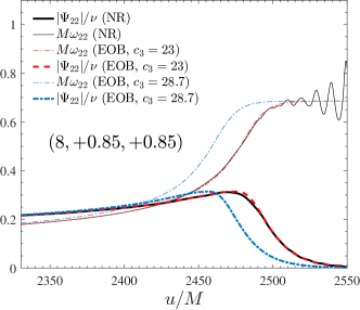
Figure 4: Effect of changing the value of the effective NNNLO spin-orbit parameter $c_{3}$ for the $(8,+0.85,+0.85)$ configuration. Time-domain evolution of frequency and amplitude. The $5.2\%$ value of $\bar{F}$ in Fig. 3 comes entirely from the value $c_{3}=28.7$ obtained by extrapolating from the SXS-based fit of Eq. (II.2.2). A smaller value of the parameter, $c_{3}=23$, succeeds in getting a good EOB/NR agreement ($\bar{F}\simeq 1.3\times 10^{-3}$) . Despite this, both the NQC and post-merger sectors are correctly represented by the model because of the robust NR-informed fits.

To explicitly see that the origin of such EOB/NR discrepancy comes from the EOB-driven inspiral dynamics and not from the ringdown part, we display in Fig. 4 the waveform frequency and amplitude versus time. The figure compares three datasets: (i) the BAM data (black); (ii) the TEOBResumS waveform with the value of $c_{3}\approx 28.7$ obtained from Eq. (II.2.2) (blue, dash-dotted, lines) and $c_{3}=23$. Note that while the $c_{3}=28.7$ waveform was obtained by iterating on NQCs parameter (i.e., the NQC correction is also added to the flux for consistency with the waveform and then an iterative procedure is set until the values of $(a_{1},a_{2})$ are seen to converge Nagar et al. (2017)), the $c_{3}=23$ one was not (see below). The waveforms are aligned in the $(0.2,0.35)$ frequency interval region. The figure clearly illustrates that the simple action of lowering $c_{3}$ (i.e. making the spin-orbit interaction less attractive, see discussion in Nagar et al. (2017)) is effective in getting the TEOBResumS waveform closer to the BAM one: the waveform becomes longer and the frequency behaviors get qualitatively more similar up to merger. Note also that the postmerger part is perfectly consistent with the NR one. This is a remarkable indication of the robustness of our post-merger fits since the $(8,+0.85,+0.85)$ BAM dataset was not used in their construction. We mentioned above that the curves corresponding to $c_{3}=23$ were obtained without iterating on the amplitude NQC parameters $(a_{1},a_{2})$. The reason for this is that the value of the NQC parameters are rather large because of the lack of robustness of the resummed waveform amplitude in this corner of the parameter space and they effectively tend to compensate the action of $c_{3}$, that should be lowered further. The consequence of this is that, when $c_{3}$ is chosen to be below 20, $(a_{1},a_{2})$ become so large that the iteration procedure is unable to converge. The use of the improved factorized and resummed waveform amplitudes of Refs. Nagar and Shah (2016); Messina et al. (2018), that display a more robust and self-consistent behavior towards merger for high, positive spins is expected to solve this problem.

To summarize, the message of the analysis illustrated in Fig. 4 goes as follows: (i) on the positive side, the figure illustrates that, even if we had not included $(8,+0.85,+0.85)$ data to obtaining the postmerger fit parameters, the resulting model is rather accurate also for this choice of parameters; (ii) on the negative side, it also tells us that the dataset $(8,+0.85,+0.85)$ brings us new, genuine, NR information that is currently not incorporated in the model, but it should be in order to properly capture the correct phasing behavior in this corner of the parameter space. In principle, improving the model would be rather straightforward, as it would just amount to adding a new value of $c_{3}$ in Table 1, corresponding to an acceptable BAM/EOB phasing up to merger, and redoing the global fit. However, because of the aforementioned problems in obtaining a consistent determination of the NQC parameters, we shall postpone this to a forthcoming study that will (partly) use the factorized and resummed waveform amplitudes of Ref. Messina et al. (2018).

Figure 5: Frequency and amplitude comparison between TEOBResumS and BAM for $(18,-0.80,0)$. The full waveform amplitude develops a slightly unphysical feature due to the action of the NQC parameters. The frequency (as well as $\bar{F}$) is unaffected by this.

Finally, Fig. 5 illustrates another difference between TEOBResumS and BAM waveforms. The figure compares the analytical and numerical frequencies and amplitudes for $(18,-0.80,0)$. The waveforms are aligned around merger. Although the frequencies are perfectly consistent, the analytical amplitude (red line) shows a qualitatively incorrect behavior before merger. Although such feature in the amplitude might be interpreted as due to an incorrect determination of the NQC corrections, it is actually of dynamical origin. More precisely, it comes from the orbital frequency $\Omega$ crossing zero and then becoming negative due to a somewhat large values of the gyro-gravitomagnetic functions $(G_{S},G_{S_{*}})$ for small values of the EOB radial separations. Since the spins are negative, the spin-orbit part of the orbital frequency progressively compensates the orbital one, until dominating over it so that $\Omega<0$ around merger time. We have tracked back the origin of this problem to the fact that, following Ref. Damour and Nagar (2014b), the argument of the functions $(\hat{G}_{S},\hat{G}_{S_{*}})$ (see Eqs. (36)-(37) of Damour and Nagar (2014b)) where chosen, by construction, to be $1/r_{c}$, instead of of $1/r$, so as to effectively incorporate higher-order spin-orbit corrections. Although it is not our intention to discuss this subject in more detail here, we have actually verified that going back to the standard $1/r$ dependence of these functions is sufficiently to reduce and/or cure completely (as it is the case for the configuration $(11,-0.95,-0.50)$ discussed below) this somewhat unphysical feature. Although the behavior of the modulus in Fig. 5 has not practical consequences, it is important to mention that similar features may occur systematically for binaries with large $q$ and large spins, anti-aligned with the orbital angular momentum. This statement will be recalled below when discussing the performance of the model outside the NR-covered region of the parameter space. Finally, a global representation of the results of Figs. 1-3 is given in Fig. 6, that displays the maximum value of the EOB/NR faithfulness $F$, reached for each dataset varying the total mass $M$, all over the SXS and BAM waveform catalogs, only excluding the $(8,+0.85,+0.85)$ outlier for readability.

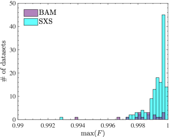
Figure 6: Global picture of the maximum value of the EOB/NR faithfulness $F$, Eq. (19) over SXS and BAM NR data. The only outlier above $3\%$, (8,+0.85,+0.85), is omitted from the figure.

II.4 Waveform robustness outside the NR-covered region of parameter space

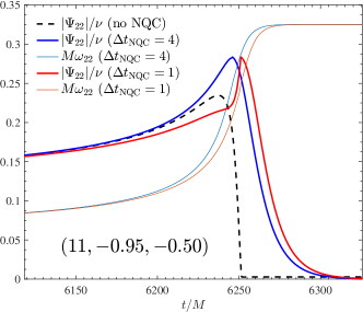
Figure 7: Comparing the effect of using $\Delta t_{\rm NQC}=1$ and $\Delta t_{\rm NQC}=4$ for $(q,\chi_{1},\chi_{2})=(11,-0.95,-0.50)$. The use of $\Delta t_{\rm NQC}=4$ makes the behavior of the waveform amplitude at merger consistent with the NR-fitted postmerger behavior.

Figure 8: Calculation of $\bar{F}$ between EOB waveforms with $\Delta t_{\rm NQC}=1$ and $\Delta t_{\rm NQC}=4$ at the boundary of the region of the parameter space defined by Eqs. (20)-(21). The consistency between the two types of waveforms is excellent.

The model was tested to be robust in the most demanding corners of the parameter space, notably for large mass ratios (though we limit ourselves to $q\leq 20$) and large values of the spin magnitudes. In particular, no obvious problem was found for large mass ratios and when the spins are positive. The absence of ill-defined behaviors in the waveform is mostly due to the use of robust fits across the whole parameter space and to the fact that the NQC corrections are able to effectively reduce the residual inaccuracies in the EOB waveform. However, this comes at the price of large NQC parameters (far from being order unity, as noted above for the specific case of $(8,+0.85,+0.85)$) since they have to strongly correct a waveform in a regime where the radial momenta are small. Large NQC parameters prevent the necessary iterative procedure of recomputing the flux from converging. We thus remove the NQC corrections to the flux, although in this way it becomes mildly inconsistent with the waveform.

As anticipated above, when the mass ratio is moderately large ($q\geq 8$) and spins are equally large but anti-aligned with the angular momentum, the waveform amplitude may develop artifacts prompted by the underlying orbital frequency being small and eventually crossing zero (and thus strongly affecting the NQC amplitude correction factor) as we found for the $(8,-0.80,0)$ configuration.

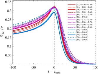
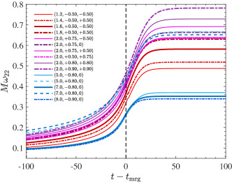
Figure 9: Sanity check of EOB waveform modulus (top) and frequency (bottom) on the configurations considered in Table I of Bohé et al. Bohé et al. (2017). Differently from what we do here, NR waveform data for these configurations were used in Bohé et al. (2017) to calibrate SEOBNRv4. The behavior of both functions look qualitatively and quantitatively consistent and robust. Waveforms are time-shifted to be all aligned at merger time.

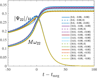
Figure 10: Sanity check of EOB waveforms for large mass ratios and large spins anti-aligned with the angular momentum. The good qualitative behavior of the waveform around merger is guaranteed by the value of $\Delta t_{\rm NQC}$ given by Eq. (20)-(21).

For example, Fig. 7 illustrate the type of, qualitatively incorrect, features that the waveform can develop towards merger due to the incorrect action of the NQC factor. In the figure we show, with a red and an orange line, the amplitude and frequency for $(11,-0.95,-0.50)$ as generated by the model described above. The black dashed line is the bare EOB-waveform amplitude, without the NQC factor. We have explicitly verified that $\Omega$ crosses zero also in this case. Although, as we mentioned above, the theoretically correct way of solving this problem is to modify the spin-orbit sector of TEOBResumS, one finds that, if the standard value $\Delta t_{\rm NQC}=1$ is increased to $\Delta t_{\rm NQC}=4$, the weird behavior disappears and the inspiral EOB waveform amplitude can be connected smoothly to the postmerger part obtained via the global fit of the NR waveform data. The same kind of EOB/NR inconsistency also appears for configurations with even higher mass ratios and large, negative, spins. In some extreme situations, it can also affect the frequency. We performed a thorough scan of the parameter space and we concluded that a pragmatical approach to solve this problem is simply to impose $\Delta t_{\rm NQC}=4$ for a certain sample of configurations. More precisely, we found that the ubiquitous $\Delta t_{\rm NQC}=1$ should be replaced by $\Delta t_{\rm NQC}=4$ when

$$8<q<11 ~{}\text{and}~{}\chi_{A}<-0.9,$$ (20)

$$11<q<19 ~{}\text{and}~{}\chi_{A}<-0.8.$$ (21)

Note that, despite being independent of the value of $\chi_{B}$, such simplified conditions allow to generate waveforms that present a sufficiently sane and smooth behavior around the merger up to mass ratio $q=20$ and spins $\chi_{A}=\chi_{B}=\pm 0.95$. Finally, the last question is about the magnitude of the uncertainty that one introduces by choosing $\Delta t_{\rm NQC}=4$ instead of $\Delta t_{\rm NQC}=1$ at the boundary of the region of the parameter space defined by Eqs. (20)-(21). We evaluated this by (i) choosing several configurations at the interface, on the $(\nu,\chi_{A})$ square, and by computing $\bar{F}$ between EOB waveforms with $\Delta t_{\rm NQC}=1$ and $\Delta t_{\rm NQC}=4$. We find values of $\bar{F}$ (see Fig. (8)) on average around $10^{-3}$, which means that having a discontinuous transition has in fact no practical consequences. Evidently, the radical solution to this problem will eventually be to change the argument of the gyro-gravitomagnetic functions $(\hat{G}_{S},\hat{G}_{S_{*}})$ as mentioned above. In this respect, we have checked that doing so for the case $(11,-0.95,-0.50)$ of Fig. 7 allows one to (i) avoid the orbital frequency $\Omega$ crossing zero and (ii) consequently recovering a qualitatively excellent modulus around merger simply keeping $\Delta t_{\rm NQC}=1$. Since such an improved TEOBResumS model will have also to rely on a different determination of $c_{3}$ to be consistent with all NR simulations, we postpone a detailed treatment to future work.

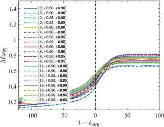
Figure 11: Sanity check of EOB waveforms amplitude (top) and frequency (bottom) for several mass ratios and large spins aligned with the orbital angular momentum. The global consistency is highly satisfactory for both amplitude and frequency.

Finally, we test the robustness of the merger waveform provided by TEOBResumS on several specific configurations. In Fig. 9 we cover that portion of the parameter space listed in Table I of Ref. Bohé et al. (2017) (and notably covered by nonpublic SXS NR simulations). In addition, Figs. 10-11 systematically explore several configurations corresponding to the conditions given by Eqs. (20)-(21). The figure stresses that neither the amplitude nor the frequency show any evident pathological behavior around merger. This makes us confident that TEOBResumS waveforms should provide a reasonable approximation to the actual waveform for that region of the parameter space. Evidently, like the case of (8,+0.85,+0.85) mentioned above, this does not a priori guarantee that, had we at hand long NR simulations for such parameters, we would get a phasing consistent with the numerical error, since modifications of $c_{3}$ might be needed. However, we think that constructing a waveform without evident pathologies is already a good achievement seen the lack of NR-based complementary information in these corners of the parameter space.

III Binary Neutron Stars

General relativity predicts that the GW signal emitted by the quasi-circular inspiral and plunge of BNSs is a chirp-like signal qualitatively similar to that of a BBH system, but modified due to the presence of tidal effects. At leading PN order, the latter arise because the gravitational field of each star induces a multipolar deformation on the companion that makes the binary interaction potential more attractive. This means that,compared to the pure space-time BBH process, the coalescence process is faster. Quadrupolar leading-order tidal interactions enter the dynamics at the 5th post-Newtonian order Damour (1983); Damour et al. (1993); Racine and Flanagan (2005); Flanagan and Hinderer (2008); Damour and Nagar (2010); Vines et al. (2011). The impact on the phase evolution, however, is significant already at GW frequencies $f_{\mathrm{GW}}\gtrsim 150\mathrm{Hz}$ Hinderer et al. (2010) and becomes the dominant effect towards the end of the inspiral Bernuzzi et al. (2014). The magnitude of the tidal interaction is quantified by a set of dimensionless tidal polarizability coefficients for each star. The dominant one is usually addressed in the literature as “tidal deformability” and is defined as

$$\Lambda_{2}=\dfrac{2}{3}k_{2}\left(\dfrac{c^{2}}{G}\dfrac{R_{*}}{M_{*}}\right)^{5},$$ (22)

where $k_{2}$ is the quadrupolar gravito-electric Love number and $(R_{*},M_{*})$ are the NS areal radius and mass Hinderer (2008); Damour and Nagar (2009); Binnington and Poisson (2009). The $\Lambda_{\ell}$ parameters are strongly dependent on the NS internal structure; thus, their measurement provides a constraint on the equation of state of cold degenerate matter at supranuclear densities. Reference Abbott et al. (2017b) provided the first measure of $\Lambda_{2}$ from GW data, setting upper limits and allowing to disfavor some of the stiffest EOS models.

III.1 Main features

Our starting point for describing the BNS evolution up to the merger is the model discussed in Ref. Bernuzzi et al. (2015a), where the point-mass $A_{0}$ potential (formerly denoted as $A(r)$) is augmented by a gravitational self-force (GSF)-informed tidal contribution Bini and Damour (2014). Following Damour and Nagar (2010), the complete EOB potential is written as

$$A=A_{0}+A_{T}^{(+)}\ ,$$ (23)

where

$$A_{T}^{(+)}(u;\nu)\equiv-\sum_{\ell=2}^{4}\left[\kappa_{A}^{({\ell})}u^{2\ell+2}\hat{A}^{(\ell^{+})}_{A}+({A}\leftrightarrow{B})\right]\$$ (24)

models the gravito-electric sector of the interaction, with $u\equiv 1/r$. In the expression above, the ${\ell}=2,3,4$ tidal coupling constants are defined as

$$\kappa_{A}^{(\ell)} =2\dfrac{X_{B}}{X_{A}}\left(\frac{X_{A}}{{\cal C}_{A}}\right)^{2{\ell}+1}k^{A}_{\ell}\ ,$$ (25a)

$$\kappa_{B}^{(\ell)} =2\dfrac{X_{A}}{X_{B}}\left(\frac{X_{B}}{{\cal C}_{B}}\right)^{2{\ell}+1}k^{B}_{\ell}\ ,$$ (25b)

in which ${\cal C}_{A,B}=M_{A,B}/R_{A,B}$ are the compactness of the two stars, $R_{A,B}$ their areal radii, while $k_{\ell}^{A,B}$ are the dimensionless relativistic Love numbers Damour (1983); Hinderer (2008); Damour and Nagar (2009); Binnington and Poisson (2009); Hinderer et al. (2010).

At leading order, tidal interactions are fully encoded in the total dimensionless quadrupolar tidal coupling constant

$$\kappa^{T}_{2}\equiv\kappa^{(2)}_{A}+\kappa^{(2)}_{B}.$$ (26)

The above parameter is key to discovering and to interpreting EOS quasi-universal relations for BNS merger quantities Bernuzzi et al. (2014, 2015b); Zappa et al. (2018). In GW experiments, however, one often measures separately $(\Lambda^{A},\Lambda^{B})$ and the masses Del Pozzo et al. (2013); Agathos et al. (2015); Abbott et al. (2017b). The expression relating $\kappa_{2}^{T}$ to $(\nu,\Lambda_{2}^{A},\Lambda_{2}^{B})$ can be easily obtained by inserting Eq. (22) into Eq. (26) and reads

$$\kappa_{2}^{T}\left(\nu;\Lambda_{2}^{A},\Lambda_{2}^{B}\right) =\dfrac{3}{8}\nu\bigg{[}\left(\Lambda_{2}^{A}+\Lambda_{2}^{B}\right)\left(1+3X_{AB}^{2}\right)$$

$$+\left(\Lambda_{2}^{A}-\Lambda_{2}^{B}\right)X_{AB}\left(3+X_{AB}^{2}\right)\bigg{]}\ .$$ (27)

The relativistic correction factors $\hat{A}^{(\ell^{+})}_{A}$ formally include all the high PN corrections to the leading-order tidal interaction. The particular choice of $\hat{A}^{(\ell^{+})}_{A}$ defines a particular TEOB model. For example, the PN-expanded next-to-next-to-leading-order (NNLO) tidal model is given by the, fractionally 2PN accurate, expression

$$\hat{A}_{A}^{(\ell^{+})}(u)=1+\alpha^{(\ell)}_{1}u+\alpha^{(\ell)}_{2}u^{2}\ \ \ {[\rm NNLO]}\ ,$$ (28)

with $\alpha^{(2),(3)}_{1,2}\neq 0$ computed analytically and $\alpha^{(4)}_{1,2}=0$ Bini et al. (2012). This TEOBNNLO model has been compared against NR simulations in Bernuzzi et al. (2012a, 2015a). Significant deviations are observed during the last 2-3 orbits before merger at dimensionless GW frequencies $M\omega_{22}\gtrsim 0.8$, that roughly correspond to the GW frequency of the stars’ contact.

The TEOBResum model is defined from TEOBNNLO by replacing the $\ell=2$ term in (28) with the expression

$$\hat{A}^{(2^{+})}_{A}(u) =1+\dfrac{3u^{2}}{1-r_{\rm LR}u}+\dfrac{X_{A}\tilde{A}_{1}^{(2^{+})\rm 1SF}}{(1-r_{\rm LR}u)^{7/2}}+\dfrac{X_{A}^{2}\tilde{A}_{2}^{(2^{+})\rm 2SF}}{\left(1-r_{\rm LR}u\right)^{p}},$$ (29)

where $p=4$ and the functions $\tilde{A}_{1}^{(2^{+})\rm 1SF}(u)$ and $\tilde{A}_{2}^{(2^{+})\rm 2SF}(u)$ are given in Bini and Damour (2014), obtained by fitting to numerical data from Dolan et al. (2015). The key idea of TEOBResum is to use as pole location in Eq. (29) the light ring $r_{\rm LR}(\nu;\kappa_{A}^{(\ell)})\,$ of the TEOBNNLO model, i.e., the location of the maximum of $A^{\rm NNLO}(r;\,\nu;\,\kappa_{A}^{(\ell)})/r^{2}$. TEOBResum is completed with a resummed waveform Damour et al. (2009) that includes the NLO tidal contributions computed in Damour and Nagar (2010); Vines and Flanagan (2010); Damour et al. (2012). TEOBResum is consistent with state-of-the-art NR simulations up to merger Bernuzzi et al. (2015a). Consistently with the BBH case, we here conventionally define the BNS merger as the peak of the $\ell=m=2$ amplitude of the strain waveform. The results of Bernuzzi et al. (2015a) span a sample of equation of states (EOS) and consequently a large range of the tidal coupling parameters. Such results were later confirmed by Hotokezaka et al. Hotokezaka et al. (2015, 2016). Similarly, Ref. Dietrich and Hinderer (2017) showed that TEOBResum is consistent with an alternative tidal EOB model that does not incorporate GSF-driven information but instead includes a way of accounting for the $f$-mode oscillations of the NS excited during the orbital evolution Hinderer et al. (2016). A ROM version of TEOBResum of Ref. Bernuzzi et al. (2015a) exists Lackey et al. (2017) and it is implemented in LAL under the name TEOBResum_ROM. In conclusion, despite a certain amount of approximations used to build the model, we take the tidal EOB-model of Ref. Bernuzzi et al. (2015a) as our current best waveform approximant for coalescing nonspinning BNS up to merger. In the next Section, we use TEOBResum as a starting point to construct a BNS waveform model that puts together both tidal and spin effects.

III.2 EOB formalism for self-spin term

The spins of the two NSs (or in general of two deformable bodies) can be easily incorporated in the formalism of Ref. Damour and Nagar (2014b). Let us describe a two-step procedure starting from the case where the spin-spin terms are not present. This corresponds to posing the centrifugal radius $r_{c}=r$ in the framework of Ref. Damour and Nagar (2014b), i.e. Eq. (7) above. In this case, moving from spinning BBHs to spinning BNSs is procedurally straightforward, since the only trivial change is to replace the point-mass potential with the tidally augmented one. The gyro-gravitomagnetic function $G_{S}$ and $G_{S_{*}}$ are the same as in the BBH case, and are resummed taking their Taylor-inverses as discussed in Damour and Nagar (2014b). A choice needs to be made for what concerns the NNNLO effective parameter $c_{3}$, that for BBHs was tuned using NR data. Here we decide to simply fix it to zero. The reason behind this choice is that $c_{3}$ is an effective correction that depends on spin-square terms that are different in BBHs and BNSs and thus it is safer to drop it here. We have indeed explored the effect of keeping the BBH value of $c_{3}$ for $\chi_{A}=\chi_{B}=0.1$ comparing with the BNS NR data corresponding to the SLy EOS and $1.35M_{\odot}+1.35M_{\odot}$. We find that such effect is not significant because it enters at high PN order in a frequency regime that is not really reached in a BNS system.

For what concerns spin-spin effects, it turns out that it is very easy to incorporate them into the EOB model at leading-order (LO) also in the presence of matter objects like NSs. When we talk of spin-spin interaction, let us recall that the PN-expanded Hamiltonian is made by three terms: the mutual interaction term, $H_{S_{A}S_{B}}$, and the two self-spins ones $H_{S_{A}S_{A}}$ and $H_{S_{B}S_{B}}$. These two latter terms originate from the interaction of the monopole $m_{B}$ with the spin-induced quadrupole moment of the spinning black hole of mass $m_{A}$ and vice versa. For a NS, the same physical effect exists, but the spin-induced quadrupole moment depends on the equation of state (EOS) by means of some, EOS-dependent, proportionality coefficient Poisson (1998). As we have seen above, for BBHs, Ref. Damour and Nagar (2014b) introduced a prescription to incorporate into the EOB Hamiltonian all three spin-spin couplings (at NLO) in resummed form, by including them inside a suitable centrifugal radius $r_{c}$. This quantity mimics, in the general, comparable-mass case, the same quantity that can be defined in the case of the Hamiltonian of a test particle around a Kerr black hole. In this latter case, this takes into account the quadrupolar deformation of the hole due to the black hole rotation. For comparable-mass binaries, this may be thought as a way of incorporating the quadrupolar deformation of each black hole induced by its rotation. At LO, the definition of the centrifugal radius of Eq. (7) simply reads

$$r_{c}^{2}=r^{2}+\hat{a}^{2}_{0}\left(1+\dfrac{2}{r}\right).$$ (30)

where we recall that the dimensionless effective Kerr spin is

$$\hat{a}_{0}=\tilde{a}_{A}+\tilde{a}_{B}$$ (31)

with $\tilde{a}_{A,B}=X_{A,B}\chi_{A,B}$. The use of these spin variables is convenient for several reasons: (i) the analytical expressions for spin-aligned binaries are nicely simplified and shorter compared to other standard notations ; (ii) in the large mass ratio limit $M_{B}\ll M_{A}$, one has that $\tilde{a}_{A}$ becomes the dimensionless spin of the massive black hole of mass $M_{A}\approx M$, while $\tilde{a}_{B}$ just reduces to the usual spin-variable of the particle $\sigma\equiv S_{B}/(M_{A}M_{B})$.

Next-to-leading order spin-spin effects can be incorporated in a different fashion depending on whether the spins are generic or aligned with the orbital angular momentum. This is still ongoing work that needs further investigation Balmelli and Damour (2015). In the case of two NSs the recipe we propose here to include spin-spin couplings at LO is just to replace the definition of the effective spin $\hat{a}_{0}$ in Eq. (30) by the following quadratic form of $\tilde{a}_{A}$ and $\tilde{a}_{B}$

$$\hat{a}_{Q}^{2}=C_{QA}\tilde{a}_{A}^{2}+2\tilde{a}_{A}\tilde{a}_{B}+C_{QB}\tilde{a}_{B}^{2}$$ (32)

where $C_{QA}$ and $C_{QB}$ parametrize the quadrupolar deformation acquired by each object due to its spin . For a black hole, $C_{Q}=1$ and in this case Eq. (32) coincides with Eq. (31). For a NS (or any other “exotic” object different from a black hole, like a boson star Sennett et al. (2017)) $C_{Q}\neq 1$ and needs to be computed starting from a certain equation of state (see below). We can then follow Ref. Damour and Nagar (2014b) and the EOB Hamiltonian will have precisely the same formal structure of the BBH case. In particular, the complete equatorial $A$ function entering $\hat{H}_{\rm orb}^{\rm eff}$ reads

$$A(r,\nu,S_{i},\kappa_{i},C_{Qi})=\left[\dfrac{1+2u_{c}}{1+2u}A_{\rm orb}(u_{c},\nu,\kappa_{i})\right]_{u_{c}(u,S_{i},C_{Qi})},$$ (33)

where $u_{c}\equiv 1/r_{c}$ is obtained from Eq. (30) and (32) and we indicated explicitly the dependence on the various EOS-dependent parameters. Note that $A_{\rm orb}$ is here depending explicitly on the tidal parameters $\kappa_{i}$, because this is meant to be the sum of the point-mass $A$ function plus the tidal part of the potential used in Ref. Bernuzzi et al. (2015a) but everything is now taken as a function of $u_{c}$ instead of $u$. One easily checks that, by PN-expanding the spin-dependent EOB Hamiltonian, as given by Eqs. (23), (24) and (25) of Damour and Nagar (2014b), the LO spin-spin term coincides with the corresponding one of the ADM Hamiltonian given in Eqs. (8.15) and (8.16) of Levi and Steinhoff (2014), that in our notation just rereads as

$$\hat{H}_{\rm ss_{\rm LO}}^{\rm ADM}=-\dfrac{1}{2r_{\rm ADM}^{3}}\left\{C_{QA}\tilde{a}_{A}^{2}+2\tilde{a}_{A}\tilde{a}_{B}+C_{QB}\tilde{a}_{B}^{2}\right\},$$ (34)

i.e $\hat{H}_{\rm ss}^{\rm ADM}=-\hat{a}_{Q}^{2}/(2r_{\rm ADM}^{3})$ using Eq. (32). Since at this PN order the useful relation between the ADM radial separation $r_{\rm ADM}$ and the EOB radial separation is just $r=r_{\rm ADM}$, it is immediate to verify the equivalence of the two results.

Incorporating the full LO spin-spin interaction in the waveform, including monopole-quadrupole terms, is similarly straightforward. First, following Ref. Damour and Nagar (2014b), Eq. (80) there, we recall that, for BBHs, this is done by including in the residual amplitude correction to the $(2,2)$ waveform a spin-dependent term of the form

$$\rho_{22}^{\rm SS_{LO}}=c^{\rm SS}_{\rm LO}x^{2}=\dfrac{1}{2}\hat{a}^{2}_{0}x^{2}.$$ (35)

The monopole-quadrupole effect is then included by just replacing $\hat{a}_{0}^{2}$ by $\hat{a}_{Q}^{2}$ from Eq. (32). One then verifies that, after PN-expanding the resummed EOB flux, the corresponding LO spin-spin term coincides with the LO term for spin-aligned, circularized binaries, given in Eq. (4.12) of Ref. Bohé et al. (2015). Such Newton-normalized, spin-spin flux contributions, once rewritten using the $(\tilde{a}_{1},\tilde{a}_{2})$ spin variables, just gets simplified as

$$\hat{\cal F}_{\rm SS}^{\rm LO}=\Bigg{\{}\tilde{a}_{A}^{2}\left(\dfrac{1}{16}+2C_{QA}\right)+\dfrac{31}{8}\tilde{a}_{A}\tilde{a}_{B}+\tilde{a}_{2}^{2}\left(\dfrac{1}{16}+2C_{QB}\right)\Bigg{\}}x^{2},$$ (36)

so that the $A\leftrightarrow B$-symmetry is apparent. This can be obtained by directly expanding the EOB-resummed flux as defined in Ref. Damour and Nagar (2014b). Actually, for this specific calculation, it is enough to consider the $(2,2)$ and $(2,1)$ waveform modes, the first at LO in the spin-spin and spin-orbit interaction, while the latter only at LO in the spin-orbit interaction. The corresponding residual amplitudes, taken from Eqs. (79), (84), (86), (89) and (90) of Damour and Nagar (2014b), read

$$\rho_{22} =\rho_{22}^{\rm orb}+\rho_{22}^{\rm S},$$ (37)

$$X_{AB}f_{21} =X_{AB}\left(\rho_{21}^{\rm orb}\right)^{2}+\tilde{f}_{21}^{\rm S},$$ (38)

where $\rho_{22}^{\rm S}$ is assumed here to incorporate only the LO spin-orbit and spin-spin contribution

$$\rho_{22}^{\rm S} =c_{\rm SO}^{\rm LO}x^{3/2}+c_{\rm SS}^{\rm LO}x^{2}$$

$$=-\left[\dfrac{\hat{a}_{0}}{2}+\dfrac{X_{AB}}{6}(\tilde{a}_{A}-\tilde{a}_{B})\right]x^{3/2}+\dfrac{1}{2}\hat{a}_{Q}^{2}x^{2},$$ (39)

$$\tilde{f}_{21}^{\rm S} =-\dfrac{3}{2}(\tilde{a}_{A}-\tilde{a}_{B}).$$ (40)

One verifies that, by keeping the orbital terms consistently, using these expressions in Eq. (74) and (75) of Damour and Nagar (2014b), one eventually obtains Eq. (36) above. As a further check, we have also verified that the use of Eq. (32) is also fully consistent with the calculation of the multipolar waveform amplitude $h_{22}$ that was done by S. Marsat and A. Bohé and kindly shared with us before publication Marsat and Bohé (2018).

At this stage, we have a complete analytical model that is able to blend, in a resummed (though approximate) way spin and tidal effects. The model is complete once all the EOS dependent information, schematically indicated by $\Lambda$ is given. More precisely, the procedure is as follows: for a given choice of the EOS, one fixes the compactness ${\cal C}$ (or the mass of the NS), which defines its equilibrium structure. Then, following Ref. Damour and Nagar (2009) (see also Refs. Hinderer (2008); Binnington and Poisson (2009); Hinderer et al. (2010)), one computes the corresponding dimensionless Love numbers $(k_{2},k_{3},k_{4})$ as they appear in the EOB potential. At this stage, the only missing piece is the EOS-dependent coefficient $C_{Q}$ for the two objects. Luckily, this can be obtained easily by taking advantage of the so-called I-Love-Q quasi-universal relations found by Yunes and Yagi Yagi and Yunes (2013a, b). In particular, following Ref. Yagi and Yunes (2013b), defining $x\equiv\log(\Lambda_{2})$ one has that, for each binary, the quadrupole coefficient $C_{Q}$ can be obtained as

$$\log\left(C_{Q}\right) =0.194+0.0936x+0.0474{x}^{2}$$

$$-4.21\times 10^{-3}{x}^{3}+1.23\times 10^{-4}{x}^{4}\ .$$ (41)

Since $C_{Q}$ is 1 for a BH but it is larger for a NS, depending on the EOS one is expecting a relevance of the monopole-quadrupole interaction terms. This was already pointed out by Poisson long ago Poisson (1998) and more recently by Harry and Hinderer Harry and Hinderer (2018).

III.3 Comparison with NR data

Table 3: Equal-mass BNS configurations considered in this work. From left to right the column reports: the EOS, the gravitational mass of each star, the compactness, the quadrupolar dimensionless Love numbers, the leading-order tidal coupling constant $\kappa_{2}^{T}$, the corresponding value of the quadrupolar “tidal deformability” for each object, $\Lambda_{2}^{A,B}$, Eq. (22), the dimensionless spin magnitude and the spin-induced quadrupole momenta $C_{QA,QB}$.

name	EOS	$M_{A,B}[M_{\odot}]$	$C_{A,B}$	$k_{2}^{A,B}$	$\kappa_{2}^{T}$	$\Lambda^{A,B}_{2}$	$\chi_{A,B}$	$C_{QA,QB}$
BAM:0095	SLy	1.35	$0.17$	0.093	73.51	392	0.0	5.491
BAM:0039	H4	1.37	$0.149$	0.114	191.34	1020.5	0.141	7.396
BAM:0064	MS1b	1.35	$0.142$	0.134	289.67	1545	0.0	8.396

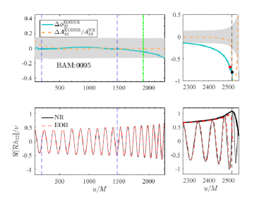
Figure 12: Phasing comparison between BAM and TEOBResumS waveforms for the SLy and Ms1b equal-mass BNS configurations of Table 3. The EOB and NR waveforms, once aligned during during the early inspiral (approximately over the first $1500M$ of evolution), are compatible, within the NR uncertainty (gray area in the figures) essentially up to the NR merger point, defined as the peak of the waveform amplitude $|h_{22}|$. Note however that the errors are larger for the MS1b configuration. The time marked by the vertical green line corresponds to 700Hz.

Figure 13: Phasing comparison between BAM and TEOBResumS waveforms, effect of spin (H4 EOS, see Table 3). The figure refers to spinning binary with dimensionless spins $\chi_{A}=\chi_{B}\approx 0.14$. NR and EOB waveforms are still compatible, within the NR uncertainty (gray area in the figures), up to the NR merger point. The time marked by the vertical green line corresponds to 700Hz.

We verify the accuracy of TEOBResumS against error-controlled NR waveforms obtained from the evolution of spinning and eccentricity reduced initial data using multiple resolutions. Initial data are constructed in the constant rotational velocity formalism using the SGRID code Tichy (2011, 2012). The residual eccentricity of the initial data is reduced to typical values $e\sim 10^{-3}-10^{-4}$ following the procedure described in Dietrich et al. (2015). The main properties of the BNS configurations discussed in this work are listed in Table 3. The initial data are then evolved with BAM Brügmann et al. (2008); *Thierfelder:2011yi using a high-order method for the numerical fluxes of the general-relativistic hydrodynamics solver Bernuzzi and Dietrich (2016).

The BAM waveforms employed here were produced and discussed in Dietrich et al. (2017a, 2018b). We perform multiple resolution runs, up to grid resolutions that allow us to make an unambiguous assessment of convergence. We find a clear second order convergence in many cases and build a consistent error budget following the convergence tests Bernuzzi and Dietrich (2016). For this work we additionally checked some of the waveforms by performing additional simulation with the THC code Radice et al. (2014a, b). The comparison with an independent code allows us to check some of the systematics uncertainties that affect BNS simulations Bernuzzi et al. (2012a); Radice et al. (2014a, b). We find that the two codes produce consistent waveforms. Results are summarized in Appendix D.

Figures 12 and 13 illustrate EOB/NR phasing comparison. The EOB waveforms are aligned, fixing a relative time and phase shift, to the NR ones in the inspiral region marked by two vertical lines on the left panels that correspond to the same frequency interval $(\omega_{L},\omega_{R})$ on both the EOB and NR time series Baiotti et al. (2011). The alignment frequency intervals are $(\omega_{L},\omega_{R})=(0.039,0.05)$ for BAM:0095; $(0.0365,0.045)$ for BAM:0039 and $(0.038,0.05)$ for BAM:0064. The shaded areas in the top panels mark the NR phasing uncertainty as estimated in Appendix D. For reference, the green, vertical line indicates the time at which the 700 Hz frequency is crossed. The figure clearly illustrates that: (i) EOB and NR waveforms are fully compatible up to our conventionally defined merger point, the peak of the $|h_{22}|$ waveform amplitude, over the full range of values of $\kappa_{2}^{T}$ considered as well as for spins. Interestingly, the leftmost panel of Fig. 12 also shows that the EOB-NR phase difference towards merger is acceptably small ($<1$ rad), but also significantly larger than the NR uncertainty. This illustrates that, for the first time, our NR simulations are finally mature to inform the analytical model with some new, genuinely strong-field, information that can be extracted from them.

The figures show that for the EOB dynamics, we typically underestimate the effect of tides in the last orbit, since the phase of the NR data is evolving faster (stronger tides). However, the opposite is true for BAM:0095. This result is consistent with the ones of Ref. Bernuzzi et al. (2015a) for the same physical configuration (but different simulations, leftmost panel of Fig. 3) where one had already the indication that for compact NS, tidal effects could be slightly overestimated with respect to the corresponding NR description. Informing TEOBResumS with the BAM simulations is outside the scope of the current work. However, we want to stress that this is finally possible with our improved simulations.

IV Contribution of self-spin terms to BNS inspiral

Now that we could show the consistency between the TEOBResumS phasing and state-of-the art NR simulations, let us investigate in more detail the effect of spins on long BNS waveforms as predicted by our model. First of all, let us recall that inspiralling BNS systems are not likely to have significant spins. The fastest NS in a confirmed BNS system has dimensionless spins $\sim 0.04$ Kramer and Wex (2009). Another potential BNS system has a NS with spin frequency of 239 Hz, corresponding to dimensionless spin 0.2. The fastest-spinning, isolated, millisecond pulsar observed so far has $\chi=0.04$. However, it is known that even a spin of  0.03 can lead to systematic biases in the estimated tidal parameters if not incorporated in the waveform model Favata (2014); Cho and Lee (2018). Those analysis are based on PN waveform models. A precise assessment of these biases using TEOBResumS is beyond the scope of the present work and will hopefully be addressed in the future. Since the most important theoretical novelty of TEOBResumS is the incorporation of self-spin effects in resummed form, our aim here is to estimate their effect in terms of time-domain phasing up to merger , notably contrasting the TEOBResumS description with the standard PN one.

Before doing so, let us mention that LO, PN-expanded, self-spin terms Poisson (1998) in the TaylorF2 Damour et al. (2001); Buonanno et al. (2009) inspiral approximant have been used in parameter-estimation studies by Agathos et al. Agathos et al. (2015), and, more recently, by Harry and Hinderer Harry and Hinderer (2018). The LO term (2PN accurate) to the frequency-domain phasing was originally computed by Poisson Poisson (1998). Currently, EOS-dependent, self-spin information is computed in PN theory up to 3.5PN order, so that one can have the corresponding 3.5PN accurate terms in the TaylorF2 approximant. Let us explicitly review their computation. Given the Fourier transform of the quadrupolar waveform as

$$\tilde{h}_{22}\equiv\tilde{A}(f)e^{-{\rm i}\Psi(f)},$$ (42)

the frequency domain phasing of the TaylorF2 waveform approximant, that assumes the stationary phase approximation, is obtained solving the integral given by Eq. (3.5) of Ref. Damour et al. (2001),

$$\Psi_{f}(t_{f})=2\pi ft_{\rm ref}-\phi_{\rm ref}+2\int_{v_{f}}^{v_{\rm ref}}(v_{f}^{3}-v^{3})\frac{E^{\prime}(v)}{\mathcal{F}(v)}dv,$$ (43)

where the parameters $t_{\rm ref}$ and $\phi_{\rm ref}$ are gauge-dependent integration constants. The $C_{Qi}$-dependent quadratic-in-spin energy and flux available in the literature at 3.5PN, the maximum PN order actually known in this particular case, are given in Refs. Marsat (2015) and Bohé et al. (2015) respectively, where their notation $\kappa_{\pm}$ corresponds to $\kappa_{+}=C_{QA}+C_{QB}$ and $\kappa_{-}\equiv C_{QA}-C_{QB}$. It is important to stress that in Ref. Levi and Steinhoff (2014) a circularized spin-spin $C_{Qi}$-dependent Hamiltonian, equivalent to the Multipolar post-Minkowskian (MPM) result of Ref. Marsat (2015) (see their Appendix D), was computed via effective field theory (EFT) techniques. From Eq. (43), by taking into account all the orbital pieces at the consistent PN order Bernard et al. (2017); Damour et al. (2016, 2015, 2014); Blanchet (2014), one gets that the self-spin contribution is given by the sum of an LO term (2PN) Poisson (1998), an NLO term (3PN) and a LO tail term (3.5PN)

$$\Psi_{\rm SS}^{\rm PN}=\Psi^{\rm PN,LO}_{\rm SS}+\Psi^{\rm PN,NLO}_{\rm SS}+\Psi^{\rm PN,tail}_{\rm SS}.$$ (44)

The LO tail term is computed here for the first time. It was obtained by expanding, at the corresponding PN order, the EOB energy and flux adapting the procedure discussed in Messina and Nagar (2017). These three terms explicitly read

$$\Psi^{\rm PN,LO}_{\rm SS} =-\dfrac{75}{64\nu}\left(\tilde{a}_{A}^{2}C_{QA}+\tilde{a}_{B}^{2}C_{QB}\right)\left(\dfrac{\omega}{2}\right)^{-1/3},$$ (45)

$$\Psi^{\rm PN,NLO}_{\rm SS} =\frac{1}{\nu}\biggl{[}\left(\frac{45}{16}\nu+\frac{15635}{896}\right)(C_{QA}\tilde{a}_{A}^{2}+C_{QB}\tilde{a}_{B}^{2})$$

$$+\frac{2215}{512}X_{AB}(C_{QA}\tilde{a}_{A}^{2}-C_{QB}\tilde{a}_{B}^{2})\biggr{]}\left(\frac{\omega}{2}\right)^{1/3},$$ (46)

$$\Psi^{\rm PN,tail}_{\rm SS} =-\dfrac{75}{8\nu}\pi\left(\tilde{a}_{A}^{2}C_{QA}+\tilde{a}_{B}^{2}C_{QB}\right)\left(\dfrac{\omega}{2}\right)^{2/3},$$ (47)

where $\omega=2\pi Mf$ denotes the circularized quadrupolar gravitational wave frequency.

To quantitatively investigate the differences between the PN-expanded and EOB-resummed treatment of the self-spin contribution to the phase, it is convenient to use the quantity $Q_{\omega}=\omega^{2}/\dot{\omega}$, where $\omega=\omega(t)$ is the time-domain quadrupolar gravitational wave frequency, $\omega\equiv d\phi/dt$, where $\phi(t)\equiv\phi_{22}(t)$ is the phase of the time-domain quadrupolar GW waveform $h_{22}(t)=A(t)e^{{\rm i}\phi_{22}(t)}$. This function has several properties that will be useful in the present context. First, its inverse can be considered as an adiabatic parameter $\epsilon_{\rm adiab}=1/Q_{\omega}=\dot{\omega}/\omega^{2}$ whose magnitude controls the validity of the stationary phase approximation (SPA) that is normally used to compute the frequency-domain phasing of PN approximants during the quasi-adiabatic inspiral. Thus, the magnitude of $Q_{\omega}$ itself tells us to which extent the SPA delivers a reliable approximation to the exact Fourier transform of the complete inspiral waveform, that also incorporates nonadiabatic effects. Let us recall Damour et al. (2012) that, as long as the SPA holds, the phase of the Fourier transform of the time-domain quadrupolar waveform $\Psi(f)$ is simply the Legendre transform of the quadrupolar time-domain phase $\phi(t)$, that is

$$\Psi(f)=2\pi ft_{f}-\phi(t_{f})-\pi/4,$$ (48)

where $t_{f}$ is the solution of the equation $\omega(t_{f})=2\pi f$. Differentiating twice this equation one finds

$$\omega^{2}\dfrac{d^{2}\Psi(\omega)}{d\omega^{2}}=Q_{\omega}(\omega),$$ (49)

where we identify the time domain and frequency domain circular frequencies, i.e., $\omega_{f}=\omega(t)$. Second, the integral of $Q_{\omega}$ per logarithmic frequency yields the phasing accumulated by the evolution on a given frequency interval $(\omega_{L},\omega_{R})$, that is

$$\Delta\phi_{(}\omega_{L},\omega_{R})\equiv\int_{\omega_{L}}^{\omega_{R}}Q_{\omega}d\log\omega.$$ (50)

Additionally, since this function is free of the two “shift ambiguities” that affect the GW phase (either in the time or frequency domain), it is perfectly suited to compare in a simple way different waveform models Baiotti et al. (2010, 2010); Bernuzzi et al. (2012a); Damour et al. (2013); Bernuzzi et al. (2015a). Then, the self-spin contribution to the PN-expanded $Q_{\omega}$ is given by three terms

$$Q_{\omega}^{\rm PN,SS}=Q_{\omega}^{{\rm SS}_{\rm PN,LO}}+Q_{\omega}^{{\rm SS}_{\rm PN,NLO}}+Q_{\omega}^{{\rm SS}_{\rm PN,tail}},$$ (51)

that are obtained from Eqs. (45)-(47) and read

$$Q_{\omega}^{{\rm SS}_{\rm PN,LO}} =-\dfrac{25}{48\nu}\left(\tilde{a}_{A}^{2}C_{QA}+\tilde{a}_{B}^{2}C_{QB}\right)\left(\dfrac{\omega}{2}\right)^{-1/3},$$ (52)

$$Q_{\omega}^{\rm SS_{PN,NLO}} =-\frac{1}{\nu}\biggl{[}\left(\frac{5}{8}\nu+\frac{15635}{4032}\right)(C_{QA}\tilde{a}_{A}^{2}+C_{QB}\tilde{a}_{B}^{2})$$

$$+\frac{2215}{2304}X_{AB}(C_{QA}\tilde{a}_{A}^{2}-C_{QB}\tilde{a}_{B}^{2})\biggr{]}\left(\frac{\omega}{2}\right)^{1/3},$$ (53)

$$Q_{\omega}^{\rm SS_{PN,tail}} =\dfrac{25}{12\nu}\pi\left(\tilde{a}_{A}^{2}C_{QA}+\tilde{a}_{B}^{2}C_{QB}\right)\left(\dfrac{\omega}{2}\right)^{2/3}.$$ (54)

Figure 14: EOS-dependent self-spin effects on the phasing through the $Q_{\omega}^{\rm SS}$ diagnostics. The figure contrasts the EOB description (incorporating LO dynamical and dissipative effects) with various PN approximations (see text) for the BAM:0095 tidal configuration with however $\chi_{A}=\chi_{B}=0.1$. The vertical lines mark respectively 400Hz, 700Hz and 1kHz. The EOB resummed description enhances the effect during most of the inspiral, though it reduces it towards merger. Consistency with all PN approximants is found in the low frequency regime (20Hz), though the PN regime is not yet reached there.

The corresponding function in TEOBResumS, $Q_{\omega}^{\rm TEOBResumS,SS}$ is computed, in the time domain, as follows. We perform two different runs, one with $C_{Qi}\neq 0$ another with $C_{Qi}=0$. In both cases we compute the time-domain $Q_{\omega}$ and finally calculate

$$Q_{\omega}^{\rm TEOBResumS,SS}\!\!=Q_{\omega}^{\rm TEOBResumS_{C_{Qi}\neq 0}}\!\!\!-Q_{\omega}^{\rm TEOBResumS_{C_{Qi}=0}}.$$ (55)

Although the procedure is conceptually straightforward, since it only requires the computation of numerical derivatives of the time-domain phase $\phi(t)$, there are technical subtleties in order to obtain a clean curve to be compared with the PN results. First of all, any oscillation related to residual eccentricity coming from the initial data, though negligible both in $\phi(t)$ or $\omega(t)$, will get amplified in $Q_{\omega}$ making the quantity useless. To avoid this drawback, the use of the 2PA initial data of Ref. Damour et al. (2013), discussed in detail in Appendix C, is absolutely crucial. Second, in order to explore the low-frequency regime one has to get rid of the time-domain oversampling of the waveform, since it eventually generates high-frequency (though low-amplitude) noise in the early frequency part of the curve. To this aim, the raw time-domain phase $\phi(t)$ was suitably downsampled (and smoothed). Since the time-domain output of TEOBResumS is evenly sampled in time (but not in frequency) such procedure had to be done separately on different time intervals of the complete signal (e.g. starting from 20Hz) that are then joined together again.

The outcome of this calculation is represented, as a black line, in Fig. 14. As case study, we selected the BAM:0095 configuration of Table 3 with $\chi_{A}=\chi_{B}=0.1$. To orient the reader, the vertical lines correspond to 400Hz, 700Hz and 1kHz. The figure illustrates two facts: (i) the EOB-resummed representation of the self-spin phasing is consistent, as it should, with the PN description when going to low-frequencies and (ii) it is stronger during most of the inspiral (i.e. more attractive). More detailed analysis of the self-spin effects in comparison with the various PN truncations displayed in the figure are discussed in Sec. VI of Ref. Dietrich et al. (2018a), to which we address the interested reader. One important information enclosed in the figure is that the difference between the EOB and NLO (3PN) description of self-spin effects is nonnegligible. It is likely that most of this difference comes from the bad behavior of the PN-expanded NLO term. Note in fact that $Q_{\omega}^{\rm SS_{\rm PN,NLO}}$ has a quite large coefficient, $15635/4032\simeq 4$, (see Eq. (IV)), that, e.g. at $M\omega\sim 0.04$, eventually yields a contribution that is comparable to the LO one in the PN series. For this reason, we are prone to think that the EOB description of self-spin effects, even if it is based only on the (limited) LO self-spin term, is more robust and trustable than the straightforward PN-expanded one. Clearly, to finally settle this question we will need to incorporate in the EOB formalism, through a suitable $C_{Qi}$-dependent expression of the $\delta\hat{a}^{2}$ given in Eq. (II.1), EOS-dependent self-spin effects at NLO. This will be discussed extensively in a forthcoming study.

V Case study: Parameter estimation of GW150914

Table 4: Summary of the parameters that characterize GW150914 as found by cpnest and using TEOBResumS as template waveform, compared with the values found by the LVC collaboration  Abbott et al. (2016c). We report the median value as well as the $90\%$ credible interval. For the magnitude of the dimensionless spins $|\chi_{A}|$ and $|\chi_{B}|$ we also report the $90\%$ upper bound. Note that we use the notation $\chi_{\rm eff}\equiv\hat{a}_{0}$ for the effective spin, as introduced in Eq. (8).

	​​​​TEOBResumS	LVC
Detector-frame total mass $M/M_{\odot}$	$73.6_{-5.2}^{+5.7}$	$70.6_{-4.5}^{+4.6}$
Detector-frame chirp mass $\mathcal{M}/M_{\odot}$	$31.8_{-2.4}^{+2.6}$	$30.4_{-1.9}^{+2.1}$
Detector-frame remnant mass $M_{f}/M_{\odot}$	$70.0_{-4.6}^{+5.0}$	$67.4_{-4.0}^{+4.1}$
Magnitude of remnant spin $\hat{a}_{f}$	$0.71_{-0.07}^{+0.05}$	${0.67}_{-0.07}^{+0.05}$
Detector-frame primary mass $M_{A}/M_{\odot}$	$40.2_{-3.7}^{+5.1}$	$38.9_{-4.3}^{+5.6}$
Detector-frame secondary mass $M_{B}/M_{\odot}$	$33.5_{-5.5}^{+4.0}$	$31.6_{-4.7}^{+4.2}$
Mass ratio $M_{B}/M_{A}$	$0.8_{-0.2}^{+0.1}$	$0.82_{-0.17}^{+0.20}$
Orbital component of primary spin $\chi_{A}$	$0.2_{-0.8}^{+0.6}$	$0.32_{-0.29}^{+0.49}$
Orbital component of secondary spin $\chi_{B}$	$0.0_{-0.8}^{+0.9}$	$0.44_{-0.40}^{+0.50}$
Effective aligned spin $\chi_{\mathrm{eff}}$	$0.1_{-0.2}^{+0.1}$	$-0.07_{-0.17}^{+0.16}$
Magnitude of primary spin $|\chi_{A}|$	$\leq 0.7$	$\leq 0.69$
Magnitude of secondary spin $|\chi_{B}|$	$\leq 0.9$	$\leq 0.89$
Luminosity distance $d_{\mathrm{L}}/\mathrm{Mpc}$	$479_{-235}^{+188}$	$410_{-180}^{+160}$

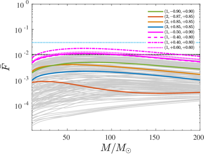
Figure 15: Unfaithfulness comparison between TEOBResumS and SXS waveforms obtained without iterating on the amplitude NQC parameters $(a_{1},a_{2})$, see Eq. (14). The performace of the model, where the parameters $(a_{6}^{c},c_{3})$ were NR-tuned with the iterative determination of $(a_{1},a_{2})$ (see Sec. II.1), is slightly worsened with respect to Fig. 1, although it is still compatible with the $1\%$ limit. Such simplified version of TEOBResumS is used for the parameter estimation of GW150914, with results reported in Table 4.

Figure 16: Reconstructed whitened GW waveforms in the Hanford (top panel) and in the Livingston (bottom panel) detectors. The solid lines indicate the median recovered waveforms. The cyan bands indicate the 90% credible regions as recovered by our analysis. As a comparison we also overlay the whitened raw strain for the two detectors.

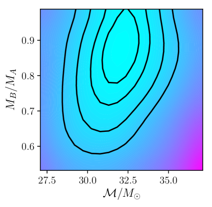
Figure 17: Two-dimensional posterior distribution for $\mathcal{M}$ and $M_{B}/M_{A}$ for GW150914 as inferred using cpnest and TEOBResumS. The contours indicate the regions enclosing $90\%$, $75\%$, $50\%$ and $25\%$ of the probability.

We test the performance and faithfulness of our waveform model in a realistic setting by performing a parameter estimation study on the 4096 seconds of publicly available data for GW150914 LOS . To do so efficiently, we do not iterate on the NQC parameters, so that the generation time of each waveform from 20 Hz is $\sim 40$ ms using the C++ version of TEOBResumS discussed in Appendix E. This worsens a bit the SXS/TEOBResumS unfaithfulness, as we illustrate in Fig. 15, though the model is still compatible with the $\max{\bar{F}}\approx 1\%$ limit and below the $3\%$ threshold. The largest value of $\bar{F}$ is in fact $\max{\bar{F}}\approx 0.018$, that is obtained for $(1,+0.40,+0.80)$. We define $\theta$ as the vector of physical parameters necessary to fully characterize the gravitational wave signal. For TEOBResumS and binary black hole systems, these are the component masses $(M_{A},M_{B})$, their dimensionless spin components $(\chi_{A},\chi_{B})$ along the direction of the orbital angular momentum, the three-dimensional coordinates in the Universe – sky position angles and luminosity distance –, polarization and inclination angles, and finally time and phase of arrival at the LIGO sites. We operate within the context of Bayesian inference; given $k$ time series of $k$ detectors’ data $d$, we construct the posterior distribution over the parameters $\theta$ as

$$p(\theta|d_{1},\ldots,d_{k},H,I)=p(\theta|H,I)\frac{p(d_{1},\ldots,d_{k}|\theta,H,I)}{p(d_{1},\ldots,d_{k}|H,I)}\,$$ (56)

where we defined our gravitational wave model – TEOBResumS – as $H$ and $I$ represents all “background” information which is relevant for the inference problem. For our choice of prior distribution $p(\theta|H,I)$, we refer the reader to Ref. Abbott et al. (2016c). Finally, we choose the likelihood $p(d_{1},\ldots,d_{k}|\theta,H,I)$ to be the product of $k$ wide sense stationary Gaussian noise distributions characterised entirely by their power spectral density, which is estimated using the procedure outlined in Ref. LOS . We sample the posterior distribution for the physical parameters of GW150914 using the Python parallel nested sampling algorithm in cpn . The cpnest model we wrote is available from the authors on request. In Table 4 we summarize our results by reporting median and $90\%$ credible intervals. These numbers are to be compared with what reported in Table I in Ref. Abbott et al. (2016c) and Table I in Ref. Abbott et al. (2016d). We also list them in the last column of Table 4 for convenience. As examples, we show the whitened reconstructed waveforms in Fig. 16 and the ${\cal M}$ and mass ratio posterior distribution in Fig. 17. We find our posteriors to be consistent with what published by the LIGO and Virgo collaborations, albeit our inference tends to prefer higher values for the mass parameters. However, no statistically significant difference is found. We find that TEOBResumS is fit to perform parameter estimation studies and that on GW150914 it performs as well as mainstream waveform models.

VI Selected comparisons with SEOBNRv4 and SEOBNRv4T

To complement the above discussion, let us collect in this section a few selected comparisons between TEOBResumS and the only other existing state-of-the-art NR-informed EOB models SEOBNRv4 and SEOBNRv4T Bohé et al. (2017); Hinderer et al. (2016); Steinhoff et al. (2016); Vines and Marsat (2018), that are currently being used on LIGO/Virgo data. The tidal sector of the SEOBNRv4T model has been recently improved so as to also include EOS-dependent self-spin terms in the Hamiltonian, though in a form different from ours, and will be discussed in a forthcoming publication. For the BBH case, our Fig. 1, when compared with Fig. 2 of Bohé et al. (2017), points out the excellent compatibility between the two models at the level of unfaithfulness with the SXS catalog of NR simulations, although the information (or calibration) of the model was done in rather different ways. For SEOBNRv4 it relies on monitoring a likelihood function that combines together the maximum EOB/NR faithfulness and the difference between EOB and NR merger times (see Sec. IVB of Bohé et al. (2017)). By contrast, the procedure of informing TEOBResumS via NR simulations relies on monitoring the EOB/NR phase differences and choosing (with a tuning by hand that can be performed in little time without the need of a complicated computational infrastructure, as explained in detail in Nagar et al. (2017)) values of parameters such that the accumulated phase difference at merger is within the SXS NR uncertainty obtained, as usual, by taking the phase difference between the two highest resolutions. This is possible within TEOBResumS because of the smaller number of dynamical parameters, i.e. $(a_{6}^{c},c_{3})$, and the rather “rigid” structure that connects the peak of the (pure) orbital frequency with the NQC point and the beginning of ringdown, Eq. (15).

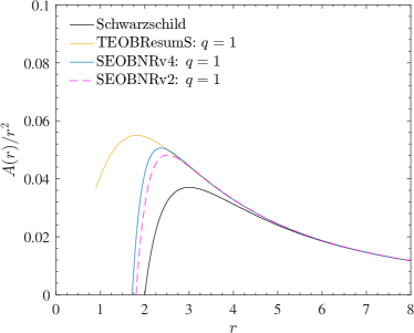
Figure 18: Comparison between two flavors of the SEOBNRv* model and TEOBResumS. The improved NR calibration incorporated in SEOBNRv4 Bohé et al. (2017); Hinderer et al. (2016); Steinhoff et al. (2016) pushed it closer to the TEOBResumS curve than the SEOBNRv2 one Taracchini et al. (2014b).

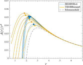
Figure 19: EOB effective photon potential $A(r)/r^{2}$ for SEOBNRv4 and TEOBResumS for mass ratios $q=(1,2,3,4,6,18)$. The potentials are consistent, though different at the peak, also for medium mass ratios. The highest consistency is found for $q=18$. The markers highlight the peaks of the functions, i.e. the locations of the effective light-rings

Figure 20: Dependence of the effective light-ring position, $r_{\rm LR}$, i.e. the peak of $A(r)/r^{2}$ in Fig. 19, versus $\nu$. The behavior of the TEOBResumS effective light-ring tends quasi-linearly to $r=3$, while the structure of the corresponding SEOBNRv4 function is more complex.

Once this is done, and in particular once one has determined a global fit for $c_{3}$, the EOB/NR unfaithfulness is computed as an additional cross check between waveforms. Here we want to make the point that, even if the models look very compatible among themselves from the phasing and $\bar{F}$ point of view, they may actually hide different characteristics. As a concrete example, we focus on the (effective) photon potential function $A/r^{2}$, where $A$ is the EOB central interaction potential. In the test-particle (Schwarzschild) limit, $A=1-2/r$ and $A/r^{2}$ peaks at the light ring $r=3$, which approximately coincides with (i) the peak of the orbital frequency; (ii) the peak of the Regge-Wheeler-Zerilli potential; (iii) the peak of the $\ell=m=2$ waveform amplitude Damour and Nagar (2007). The location of the effective light ring (or the peak of the orbital frequency) is a crucial point in the EOB formalism, since, as in the test-particle limit, it marks the beginning of the postmerger waveform part eventually dominated by quasi-normal mode ringing. We recall that TEOBResumS and SEOBNRv4 resum the $A$ potential in different ways: it is a (1,5) Padé approximant for TEOBResumS, while it is a more complicated function resummed by taking an overall logarithm for SEOBNRv4 Barausse and Buonanno (2010). Moreover, while TEOBResumS includes a 5PN-accurate logarithmic term, SEOBNRv4 only relies on 4PN-accurate analytic information. In addition, both functions are NR-modified by a single, $\nu$-parametrized function that is determined through EOB/NR phasing comparison. This is the 5PN effective correction $a_{6}^{c}(\nu)$ mentioned above for TEOBResumS and the function $K_{0}(\nu)$ for SEOBNRv4. Explicitly, we are using $a_{6}^{c}(\nu)=3097.3\nu^{2}-1330.6\nu+81.38$ and $K_{0}=+267.788247\nu^{3}-126.686734\nu^{2}+10.257281\nu+1.733598$. As a first comparison, we plot in Fig. 18 the $q=1$ effective photon potential. Right to the point, the figure illustrates that the two potentials are nicely consistent among themselves, although the structure close to merger is different. The figure also includes the potential of the SEOBNRv2 model Taracchini et al. (2014b), a model that has been used on GW150914 and that was characterized by $K_{0}=103.2\nu^{3}-39.77\nu^{2}-1.804\nu+1.712$. Interestingly, the plot shows that the *v4 potential peak is closer to the TEOBResumS one than the *v2 one. This finding deserves some mention for several reasons. First, the TEOBResumS nonspinning $A$ function behind the photon potential of Fig. 18 was NR-informed in Ref. Nagar et al. (2016) with the same nonspinning SXS NR simulations used for SEOBNRv2 (plus a $q=10$ dataset that became available after Ref. Taracchini et al. (2014b)). Second, SEOBNRv2 uses only linear-in-$\nu$ 4PN information Barausse et al. (2012); Bini and Damour (2013) while SEOBNRv4 uses the full 4PN information Damour et al. (2015, 2016), as for TEOBResumS. However, to our understanding, the SEOBNRv4 potential was also calibrated using more nonspinning NR simulations (notably with $q\gtrsim 1$) than for SEOBNRv2 (see Ref. Bohé et al. (2017)) and TEOBResumS. This suggests that the TEOBResumS potential seems able to naturally incorporate some amount of strong-field information that needs to be extracted from NR when a SEOBNRv*-like Barausse and Buonanno (2010) potential is employed. These findings merit further investigation.

In Fig. 19 we display the same comparison (though after omission of the SEOBNRv2 curve) for different mass ratios, $q=(1,2,3,4,6,18)$. One sees that both TEOBResumS and SEOBNRv4 curves are smoothly and consistently connected to the Schwarzschild case. This accomplishes the basic paradigm of the EOB formalism that the dynamics of the two-body problem is a continuous deformation of the dynamics of a test-mass on a Schwarzschild black hole Buonanno and Damour (1999, 2000), so that this limit should be properly incorporated by construction in the model and should be preserved by the addition of NR information. However, the way the Schwarzschild limit is reached is rather different in the two models. This is highlighted very well by the markers in Fig. 19. These markers indicate the location of the effective light-ring, $r_{\rm LR}$, that is shown, versus $\nu$, in Fig. 20. The figure highlights that, while the $r_{\rm LR}(\nu)$ is approximately linear for TEOBResumS (i.e. the Schwarzschild light-ring is reached at constant speed in the space of the nonspinning configurations parametrized by $\nu$) the behavior of the corresponding quantity in SEOBNRv4 is more complicated, notably it is not monotonic in $\nu$. This is not necessarily a problem from the practical point of view of generating NR-calibrated waveforms that are consistent with NR simulations. However, from the theoretical point of view, this suggests a slight inconsistency within the model, because the location of $r_{\rm LR}$ for $\nu=0.25$ is the same as for $\nu\approx 0.09$. A priori, as it was pointed out in the foundation of the EOB model Buonanno and Damour (2000); Damour et al. (2000), one would expect that the location of the LR is simply monotonically pushed to smaller radii (i.e. higher frequency) due to the repulsive effect of the higher PN $\nu$-dependent corrections that exist both at 2PN and at 3PN order. This is also suggested by NR simulations, where one finds that the GW frequency at merger (that in the EOB formalism is connected with the peak of the effective photon potential) is monotonically growing with $\nu$ (see e.g. Fig. 3 of  Healy et al. (2017)). By contrast, TEOBResumS seems to consistently incorporate this feature by construction, even with the NR-informed function $a_{6}^{c}(\nu)$. However, one sees that $r_{\rm LR}(\nu)$ is a quasi-linear function, though not exactly a straight line. This suggests that it would be interesting to investigate to which extent one can take it as a straight line (since it depends on $a_{6}^{c}$) and how this influences the EOB/NR phasing performances. We hope to address these questions in future work. As a last remark, we note that one can just plug the SEOBNRv4 $A$ interaction potential within the TEOBResumS infrastructure and, without changing anything else in the model, see whether or not the differences of Fig. 19 reflect on the waveform. It is easily found that, especially when $q>1$, the dynamics yielded by the two NR-informed potentials are rather different (and somehow not compatible), non-negligibly affecting the phasing. A detailed comparison of these aspects is interesting, and will be possibly undertaken in future work.

As additional comparison between different EOB-based waveform models, we also computed the faithfulness (or match) $F$ between TEOBResumS and SEOBNRv4T, i.e., the tidal version of SEOBNRv4 Hinderer et al. (2016); Steinhoff et al. (2016). It has to be noticed that SEOBNRv4T is conceptually different from TEOBResumS in that the effects of enhancement of the tidal interaction due to couplings with the internal oscillation $f$-mode of the stars is incorporated in the model Flanagan and Hinderer (2008); Steinhoff et al. (2016). In addition, it also includes EOS-dependent spin-spin terms, though not in the resummed form involving the centrifugal radius Vines and Marsat (2018). As above, the match here is the overlap maximized over the time (time shift) and fiducial constant phase . The comparison was done in the part of the parameter space that we expect to be astrophysically more relevant, namely, we randomly draw parameters from the uniform distributions in the mass ratio $M_{A}/M_{B}\in[1,2]$, the heaviest mass $M_{A}\in[1,3]M_{\odot}$, the spins (along orbital angular momentum) $\chi_{A,B}\in[-0.15,0.15]$, and the tidal parameters for each body $\Lambda_{A,B}\in[2,1600]$. Each waveform is computed from a nominal initial frequency of 40 Hz. The most representative results are given in Fig. 21 where we show the points drawn in the $(\Lambda_{A},M_{A})$ and $(\Lambda_{B},M_{B})$ planes. The match values, that are very high, are color-coded. The lowest match value found is 0.9898.

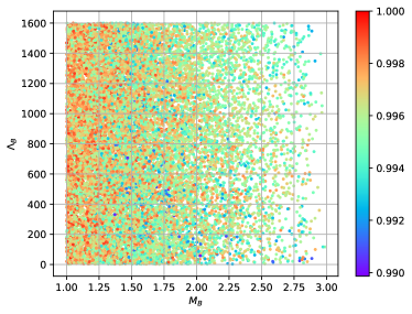
Figure 21: The match computed between SEOBNRv4T and TEOBResumS. The match values are color-coded. Based on 17300 randomly chosen points. The plot highlights the high compatibility between the two models.

Table 5: Initial conditions used to start the two EOB dynamics behind the waveforms of Fig. 22 which yield the lowest match value 0.9898. The initial frequency was nominally fixed to be 40Hz in both models. From left to right we have: the name of the model; the initial relative separation; the corresponding value of the angular momentum; the corresponding value of the circular angular momentum and the value of the radial momentum. The initial values of the phase-space variables corresponding to 40Hz are slightly different in the two models. Due to the Newtonian relation between frequency and radius that we use in TEOBResumS, Eq. (57), the consistency between initial configurations is recovered thanks to a slight modification in the initial nominal frequency of TEOBResumS so that the values of $r_{0}/M$ coincide up to the 5th decimal digit. See text for details.

Model	$f_{0}$ [Hz]	$r_{0}$	$p_{\varphi}$	$p_{\varphi}^{\rm circ}$	$p_{r}$
TEOBResumS	40.000000	50.230212	7.3060375	7.3060378	$-2.2938\times 10^{-5}$
SEOBNRv4T	40.000000	50.296059	7.3105268	7.3105268	$-2.2856\times 10^{-5}$
TEOBResumS	39.921474	50.296059	7.3105277	7.3105279	$-2.2848\times 10^{-5}$

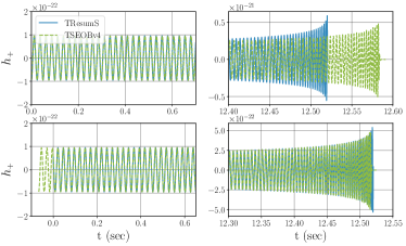
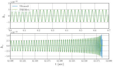
Figure 22: Time-domain comparison between SEOBNRv4T and TEOBResumS for the case that delivers the lowest match, $F=0.9898$. Top panel: same initial nominal frequency, first two lines of Table 5, the two waveforms are aligned by choosing a suitable relative time and phase shift. The first two rows of the plot show the waveforms before alignment, while the second ones after the alignment. Bottom panel: initial data for TEOBResumS consistent with those of SEOBNRv4T, see second and third row of Table 5. The two waveforms nicely agree directly, without the need of the additional alignment.

To better clarify the meaning of Fig. 21 with complementary information, we also depict in Fig. 22 the direct time-domain comparison between the two waveforms corresponding to the lowest match value, $F=0.9898$. The parameters of this binary are $M_{A}=2.99173181168$, $M_{B}=1.54656708774$, $\chi_{A}=-0.00403135733793$, $\chi_{B}=0.104676230478$, $\Lambda_{A}^{2}=1595.82370308$, $\Lambda_{B}^{2}=410.054257357$. The corresponding values the spin-induced quadrupoles are $C_{QA}=8.47884798$ and $C_{QB}=5.56870361$. The top panel of Fig. 22 shows the two $h_{+}$ waveforms without any relative time and phase shift. This is instead done in the bottom panel, with these shifts dictated by the match calculation. One notes that, although the initial GW frequency of the wave is chosen to be 40 Hz for both models (and the waves seem to consistently start in the same way) the initial conditions between the two models are different, as highlighted in Table 5. This difference comes from the relation that connects the initial frequency $f_{0}$ to the initial radius $r_{0}$. For TEOBResumS, for simplicity, one is using the simple (though approximate in this context) Newtonian Kepler’s law

$$r_{0}=\left(\dfrac{\pi fMG}{c^{3}}\right)^{-2/3}.$$ (57)

On the contrary, SEOBNRv4T correctly recovers $r_{0}$ from Hamilton’s equations (see Eqs. (4.8)-(4.9) of Ref. Buonanno et al. (2006)). The difference in $r_{0}$ is then responsible for the difference in the other phase-space variable, that is mostly behind the accumulated time-domain relative dephasing between the two waveforms highlighted in Fig. 22. By contrast, what is not relevant for this case is the fact that, while TEOBResumS implements 2PA initial data Damour and Nagar (2008); Damour et al. (2013) (see also Appendix C) SEOBNRv4T only uses the post-adiabatic (PA) approximation Buonanno and Damour (2000). Note that the effect of the 2PA correction is very small at 40 Hz, since $p_{\varphi}^{\rm circ}$ is only changed at the 7th decimal digit (see first row of Table 5). The last row of Table 5 illustrates that, if $f_{0}$ is slightly changed so to compensate for the relativistic corrections that are not included in Eq. (57) and make TEOBResumS start at the same initial radius of SEOBNRv4T, the fractional difference between the angular momenta is $\sim 10^{-7}$ and between the radial momenta is $\sim 10^{-4}$. The TEOBResumS waveform corresponding to the last row of Table 5 is now largely more consistent with the SEOBNRv4T even without time and phase alignment (see bottom panel of Fig. 22). The corresponding value of the match remains unchanged.

Since the C++ implementation of TEOBResumS that was used in Abbott et al. (2018a) was setting up the initial conditions using the simplified relation given by Eq. (57) above, we have decided not to modify it in the publicly available version of this code (see Appendix E below). By contrast, we are using a more correct relation between frequency and radius in the corresponding C implementation of TEOBResumS: the radius is obtained by solving Eq. (11a) for a given orbital frequency (assumed to be half of the nominal initial gravitational wave frequency). In this way, we can greatly improve the agreement with the corresponding SEOBNRv4T initial conditions. As an example, considering the case discussed above and detailed in Table 5, the initial radius obtained in this way is found to be $r_{0}=50.296014$.

VII Conclusions

This paper has introduced and detailed TEOBResumS, a state-of-the-art effective-one-body model that generates time-domain gravitational waveforms for nonprecessing, coalescing relativistic binaries. Our main results are as follows.

• After correcting a minor coding error in the numerical implementation of the BBH sector of the model, we obtained a new determination of the NNNLO spin-orbit effective parameter $c_{3}$ with respect to Ref. Nagar et al. (2017). In addition, the merger and postmerger part was updated with respect of Ref. Nagar et al. (2017) thanks to new effective fits that combine together NR information with test-particle results Nagar and Gunnar (2018). The parameter $c_{3}$ is determined by comparing EOB waveforms with 27, spin-dependent, NR waveforms from the SXS catalog. The model is then validated by computing the unfaithfulness (or mismatch) $\bar{F}$ over 135 NR waveforms from the SXS catalog obtained with the SpEC code and 19 NR waveforms from the BAM code. Over the SXS catalog, $\max(\bar{F})\lesssim 2.5\times 10^{-3}$ except for a single outlier, $(3,+0.85,+0.85)$ where $\max(\bar{F})\lesssim 7.1\times 10^{-3}$. By incorporating more flexibility in the global fit for $c_{3}$, notably allowing $c_{3}$ to depend quadratically on the individual spin variables also away from the equal-mass, equal-spin regime, one finds that $\max(\bar{F})\lesssim 2.5\times 10^{-3}$ all over the SXS waveform catalog. By contrast, $\bar{F}$ over the BAM NR waveform is always well below the $1\%$ level except for the single outlier $(8,+0.85,+0.85)$, that shoots up to $5.2\%$. We have identified the cause of this discrepancy to be the strength of the EOB-predicted spin-orbit interaction to be too small (i.e., resulting in a dynamics plunging too fast with respect to the NR prediction) in that corner of the parameter space. We have shown that the problem can be fixed by a new, NR-driven, choice for $c_{3}$. For simplicity, we have however decided not to provide a new fit of $c_{3}$ that also incorporates this strong-field information. This will be done in a forthcoming study that implements the factorized and resummed waveform amplitudes of Refs. Nagar and Shah (2016); Messina et al. (2018) that are expected to be more robust for large mass ratios and large, positive spins.

• We comprehensively explored the behavior of TEOBResumS waveform amplitude and frequencies outside the NR-covered portion of the parameter space. Thanks to the robustness of the merger and postmerger fits of Ref. Nagar and Gunnar (2018), the waveforms look sane and consistent among themselves even for large mass ratios ($q\leq 20$) and high-spins $(\chi 1=\chi_{2}=\pm 0.95)$.

• Building on previous work Bernuzzi et al. (2015a), the matter-dependent sector of TEOBResumS blends together, in resummed form, spin-orbit, spin-spin and tidal effects. Notably, the EOS-dependent self-spin effects are also incorporated in the model (at leading order) in a similar fashion to the BBH case Damour and Nagar (2014b). We showed that TEOBResumS waveforms are compatible with state-of-the-art, long-end, error-controlled, NR simulations of coalescing, spinning BNSs for an illustrative choice of EOS.

• We have produced selected comparisons with the EOB-based models SEOBNRv4 and its tidal counterpart, SEOBNRv4T. In particular, for the case of spinning BNS, we computed the faithfulness (or match) between SEOBNRv4T and TEOBResumS, starting from 40Hz, with $M_{A}/M_{B}\in[1,2]$, the heaviest mass $M_{A}\in[1,3]M_{\odot}$, dimensionless spins $\chi_{A,B}\in[-0.15,+0.15]$ and tidal parameters $\Lambda_{A,B}\in[2,1600]$. We found excellent compatibility between the two models, with minimum match equal to 0.9898 for more than 17,000 events.

• Finally, we tested the performance of TEOBResumS in a realistic setting by performing a parameter estimation study on the publicly available data for GW150914. Our posteriors, listed in Table 4, are fully compatible with those inferred by the LVC analysis of Refs. Abbott et al. (2016c, d), that are based on other NR-calibrated EOB waveform models.

While this paper was being finalized, a computationally efficient version of TEOBResumS based on the post-adiabatic approximation appeared Nagar and Rettegno (2018). In addition, TEOBResumS is being used to test the RIFT algorithm to perform Rapid parameter (RapidPE) inference of gravitational wave sources via Iterative Fitting Lange et al. (2018). In particular, RapidPE results obtained using TEOBResumS on GW170817 data are reported in Ref. Abbott et al. (2018a).

Appendix A An extreme BBH configuration: $(8,-0.90,0)$

After the work of the main body of this paper was finalized, we realized that the SXS collaboration had publicly released one very interesting dataset, SXS:BBH:1375 Hinder et al. (2018) with $(8,-0.90,0)$. This is interesting because it allows us to test TEOBResumS in the most difficult region of the parameter space (i.e., when the spins are anti-aligned with the orbital angular momentum) and, notably, it is marginally outside the portion covered by the BAM simulations of Table 2 for $q=8$. In fact, it has $\hat{S}=-0.7111$, to be compared with $\hat{S}=-0.6821$ corresponding to $(8,-0.85,-0.85)$.

Figure 23: Phasing comparison between TEOBResumS and SXS dataset SXS:BBH:1375. Alignment in the early inspiral (vertical lines). A EOB-NR phase difference of $-1.3$ rad is accumulated up to NR merger.

The phasing comparison is illustrated in Fig. 23. We do the following remarks. First, one sees that the phase difference (blue line) oscillates around zero. This oscillation reflects the residual eccentricity of the SXS waveform. Though it is rather small (i.e. $\sim 1.1\times 10^{-3}$) it is visible because the TEOBResumS waveform is started with essentially eccentricity free initial data because of the 2PA approximation (see Appendix C below). Second, the two waveforms dephase of about 1 rad up to the NR merger, with the TEOBResumS plunging slightly slower than the SXS one. The physical meaning of this plot is, for example, that the spin-orbit coupling in TEOBResumS is not strong enough. In our current framework, this is understood as that the value of $c_{3}$ deduced by fitting the choices of Table 1 might be (slightly) too large. Before pushing this reasoning further, let us focus on Fig. 24, that illustrates the nice agreement between the frequency and amplitude when the two waveforms are aligned around merger, on a frequency interval (0.2,0.3).

Figure 24: Complement to Fig. 23: excellent agreement between amplitude and frequency once the TEOBResumS and SXS waveforms are aligned around merger.

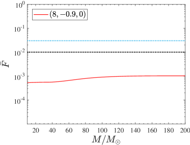
Figure 25: Unfaithfulness calculation for the system of Fig. 23. One finds that $\max{(\bar{F}})=0.001027$

Note in passing that the oscillation in the frequency is physical and is due to the beating between positive and negative frequency quasi-normal-modes Bernuzzi and Nagar (2010). This well-known feature is currently not included in the EOB model. As a last check, we computed, as usual, the EOB/NR unfaithfulness, Fig. 25. One finds that $\max{(\bar{F}})=0.001027$. This makes us conclude that, even if the time-domain analysis suggests that the value of $c_{3}$ should be slightly reduced, we are not going to do it now since the value of $\bar{F}$ is already one order of magnitude smaller than the usual target of $0.01$.

Appendix B Black-hole – Neutron-star binaries

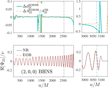
Figure 26: Phasing (left) and amplitude and frequency comparison (right) between TEOBResumS and BHNS:0002 waveform for a BHNS merger with mass ratio $q=2$, with $M_{B}=1.4M_{\odot}$. Reference Hinderer et al. (2016) indicates that the accumulated phase errors to merger are about$\sim\pm 0.5$ rad. The TEOBResumS tidal waveform is well consistent with the NR one up to merger, even in the presence of tidal disruption.

In this appendix we discuss the performances of TEOBResumS for the description of BH-NS waveforms. We stress that the model has not been developed for this type of waveforms and that this comparison is preliminary to a forthcoming investigation. We focus on the two public SXS datasets BHNS:0001 and BHNS:0002 that refer to a $q=2$ and $q=6$ nonspinning binaries where the NS is described by a $\Gamma=2$ polytropic EOS with $K=101.45$ and $K=92.12$ respectively. The dimensionless Love numbers are $k_{2,3,4}=(0.07524,0.0220429,0.0089129)$ and $k_{2,3,4}=(0.0658832,0.01873168,0.007341026)$ and the NS compactness $C_{B}=0.144404$ and $C_{B}=0.1563007$. The corresponding tidal parameters are $\Lambda_{2,3,4}=(470.8450,1095.9415,2511.5797)$ (BHNS:0001) and $\Lambda_{2,3,4}=(798.8698,2244.6773,6217.96765)$ (BHNS:0002). The values of the tidal coupling constant are $\kappa_{2}^{T}=0.50426$ for BHNS:0001 and $\kappa_{2}^{T}=19.725$ for BHNS:0002. Given the very small value of $\kappa_{2}^{T}$ for BHNS:0001, and following the reasoning of Ref. Damour and Nagar (2010) (see discussion related to Table I), we expect that dataset to behave essentially like a BBH binary with the same mass ratio.

Let us focus first on the $q=2$ binary, BHNS:0002 Fig. 26. This binary dynamics is characterized by tidal disruption that suppresses the ringdown oscillation after merger. The left panel of the figure illustrates that TEOBResumS with tides and no NQC captures well the waveform up to merger, with a phase difference of $\sim-0.3$ rad there. The “glitch” around $u/M\sim 1300$ is in the Lev3 NR data (notably not in the Lev2 ones), it is perhaps due to a re-gridding, but it is not relevant for our comparison. The phase uncertainty at merger, estimated by just taking the difference between Lev3 and Lev2 resolutions SXS , is of the order of 0.1 rad. This is of the order of the error budget at merger estimated in Ref. Hinderer et al. (2016), see Fig. 2 and Fig. 3 there, that is of the order of $\pm 0.5$ rad. Hence, the BHNS waveform obtained with TEOBResumS with tides is in agreement with the NR data up to NR merger. Our result is comparable to those presented in Ref. Hinderer et al. (2016), but we stress here that we do not use NQC-calibration and that the model only depends on the single parameter $a_{5}^{c}(\nu)$ informed by BBH data; TEOBResumS is not fed by any strong-field information extracted from the BHNS:0002.

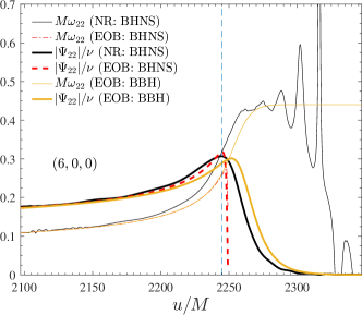
Figure 27: Left panel: TEOBResumS and NR phasing for BHNS:0001, with $q=6$ and $M_{B}=1.4M_{\odot}$. A phase difference of $\simeq-1.6$ rad is accumulated up to merger. Right panel: frequency and amplitude plot. The orange line corresponds to the TEOBResumS BBH (point-mass, no tides) waveform completed with NQC corrections and ringdown. Note that the frequency growth with tides (red-dashed) is almost indistinguishable from the corresponding curve without tides.

Figure 27 refers to the BHNS binary with larger mass ratio, $q=6$. To our knowledge, this is the first time an EOB/NR comparison is done for this dataset, as it was not included in Refs. Hinderer et al. (2016); Steinhoff et al. (2016). The phasing analysis (left panel of Fig. 27, alignment in the early inspiral) is telling us that the EOB/NR phase difference is around $-1.6$ rad at NR merger. The right panel illustrates that the TEOBResumS tidal waveform (red lines) is sane, notably with value of the merger amplitude very close to the NR one. On the same right panel we also superpose the $q=6$ BBH TEOBResumS amplitude and frequency (orange lines). This waveform has no tidal effects, but it is completed by NQC and postmerger-ringdown. Once the TEOBResumS BBH waveform is aligned to the SXS, see Fig. 28 one appreciates the high compatibility between the two waveforms during the plunge and merger, consistently with the analytical understanding that a BHNS system with $\kappa_{2}^{T}=0.50426$ is almost a BBH binary. This brings also us to the conclusion that most of the EOB/NR dephasing found in the phasing comparison of Fig. 27 is very likely not physical, but of numerical origin. Due to the lack of different resolutions in the SXS catalog (notably the Lev2 dataset was incomplete) we could not compute and estimate of the numerical error on the BHNS:0001 waveform.

We conclude that the current design of TEOBResumS is very robust and does not lead to unphysical features in extreme regions of the binary parameters. Hence, TEOBResumS is a good starting points for future BH-NS development. We also suggest that, lacking an accurate model for BH-NS, TEOBResumS can be used for the analysis of BH-NS by turning on tides in the regime $1\leq q\lesssim 4-6$ while simply using the BBH waveform for larger mass-ratios.

Figure 28: Comparison between SXS BHNS waveform (black) with the TEOBResumS BBH waveform (orange) without tides. Waveforms are aligned around merger. The suppression of the tidal interaction due to the effect of the large mass ratio is such that very little differences between the frequency and amplitude are seen.

Appendix C Post-post-adiabatic initial data for EOB dynamics

In this Appendix we discuss in detail the post-post-adiabatic prescription Damour et al. (2013) for generating initial data for the EOB dynamics. This is a crucial input that allowed us, among many things, to accurately compute the self-spin contribution to the $Q_{\omega}$ diagnostic, $Q^{\rm SS}_{\omega}$, in Fig. 14. This was also crucial to properly extract the corresponding tidal content of TEOBResumS so to compare and contrast it with the NRtidal approximant Dietrich et al. (2017a) in Ref. Dietrich et al. (2018a).

Let us consider the EOB dynamics as described in Sec. II.1. To obtain circular orbits, we set $\hat{{\cal F}}=0$ and we calculate the angular momentum $j_{0}$ at a given radius $r_{0}$ solving the equation $\partial\hat{H}_{\rm EOB}/\partial r=0$ for $p_{\varphi}$. The explicit expression of $j_{0}$ is obtained solving

$$\Bigg{\{}\Big{[}\Big{(}\frac{A}{r_{c}^{2}}\Big{)}^{\prime}\Big{]}^{2}-\frac{4A}{r_{c}^{2}}\Big{[}\tilde{G}^{\prime}\Big{]}^{2}\Bigg{\}}j_{0}^{4}+$$

$$+\Bigg{\{}2A^{\prime}\Big{(}\frac{A}{r_{c}^{2}}\Big{)}^{\prime}-4A\Big{[}\tilde{G}^{\prime}\Big{]}^{2}\Bigg{\}}j_{0}^{2}+\Big{[}A^{\prime}\Big{]}^{2}=0,$$ (58)

where $\tilde{G}\equiv G_{S}\hat{S}+G_{S_{*}}\hat{S}_{*}$. The idea behind the post-adiabatic (or post-circular) approximation is to use the fact that, when the orbital separation is large, the gravitational wave fluxes are small. We can then consider

$$\hat{{\cal F}}_{\varphi}=\bar{{\cal F}}_{\varphi}\ \varepsilon,$$ (59)

where $\varepsilon$ is a, formal, small parameter. The quasi-circular inspiralling solution of the EOB equations of motions can then be expanded as

$$p_{\varphi}^{2}= \ j_{0}^{2}\big{(}1+k_{2}\ \varepsilon^{2}+{\cal O}[\varepsilon]^{4}\big{)},$$ (60)

$$p_{r_{*}}= \ \pi_{1}\ \varepsilon+{\cal O}[\varepsilon]^{3}.$$ (61)

We now approximate $dp_{\varphi}/dt=(dp_{\varphi}/dr)(dr/dt)\sim(dj_{0}/dr)(dr/dt)$, in which we substitute Hamilton’s equations. Keeping into account only the terms linear in $p_{r_{*}}$ in Eq. (11), we get

$$\pi_{1}\varepsilon=\hat{{\cal F}}_{\varphi}\Bigg{[}\frac{\nu\hat{H}_{\rm EOB}\hat{H}_{\rm eff}^{\rm orb}\Big{(}\frac{A}{B}\Big{)}^{-1/2}}{\frac{dj_{0}}{dr}\Big{\{}1+\hat{H}_{\rm eff}^{\rm orb}\ j_{0}\Big{[}\frac{\partial\tilde{G}}{\partial p_{r_{*}}}\Big{]}_{1}\Big{\}}}\Bigg{]}_{0},$$ (62)

where the subscript $0$ indicates that the term within brackets must be evaluated at $\varepsilon=0$, for example $[\hat{H}_{\rm eff}^{\rm orb}]_{0}=\sqrt{A(1+j_{0}^{2}/r_{c}^{2})}$. Here, $[\partial\tilde{G}/\partial p_{r_{*}}]_{1}$ denotes the coefficient of the term linear in $p_{r_{*}}$ of $\partial\tilde{G}/\partial p_{r_{*}}$. Finally, $\pi_{1}\varepsilon$ constitutes the post-adiabatic approximation and the first non-zero correction to $p_{r_{*}}$. Using this result, we can calculate the post-post-adiabatic approximation (2PA) to $p_{\varphi}^{2}$. We thus solve $dp_{r_{*}}/dt\sim d(\pi_{1}\varepsilon)/dt$, in which we substitute Eq. (11) to the left hand side. This is a quadratic equation in $p_{\varphi}$ given by

$$\Big{(}\frac{A}{r_{c}^{2}}\Big{)}^{\prime}p_{\varphi}^{2}+2\big{[}\hat{H}_{\rm eff}^{\rm orb}\big{]}_{0}\Big{(}G_{S}^{\prime}\hat{S}+G_{S_{*}}^{\prime}\hat{S}_{*}\Big{)}p_{\varphi}+A^{\prime}+$$

$$+z_{3}\big{(}\pi_{1}\varepsilon\big{)}^{4}\Big{(}\frac{A}{r_{c}^{2}}\Big{)}^{\prime}+\Big{(}\frac{A}{B}\Big{)}^{-1/2}2\nu\big{[}\hat{H}_{\rm EOB}\hat{H}_{\rm eff}^{\rm orb}\big{]}_{0}\frac{d[\pi_{1}\varepsilon]}{dt}=0,$$ (63)

in which we approximated the Hamiltonians with their circular values and $p_{r_{*}}$ with $\pi_{1}\varepsilon$. Then, the derivative $d[\pi_{1}\varepsilon]/dt$ is numerically computed as $(d[\pi_{1}\varepsilon]/dj)(dj/dt)=(d[\pi_{1}\varepsilon]/dj)\ {\cal F}_{\varphi}$. We could in principle keep going and calculate the post-post-post-adiabatic correction to $p_{r_{*}}$ by reiterating the same procedure using the computed $p_{\varphi}$ in place of the circular approximation $j_{0}$.

Appendix D Error budget and systematic uncertainties in NR BNS waveforms

The error budget of the BAM BNS waveform is computed following the method developed in Bernuzzi et al. (2012b); Bernuzzi and Dietrich (2016). We perform simulations and convergence tests to identify the resolutions at which the results are in the convergent regime. Figure 29 shows an example of self-convergence test for the GW phase in which differences between data sets at different resolutions are plotted and rescaled by the factor relative to second order convergence. The lowest resolution run, in which the NS are covered with grid spacing $h=0.235$, does not give convergence results. Higher resolutions are instead in the convergent regime as indicated by the fact that dashed lines overlap with solid lines. We thus choose the convergent data and perform a Richardson extrapolation assuming second order convergence. The truncation error $\delta\phi^{\rm h}_{22}$ is estimated as the difference between the Richardson extrapolated phase and the highest resolution run.

Another source of uncertainty is that GW are extracted on spheres of finite radius. To estimate such uncertainty, we pick waveforms from the highest resolution run and from coordinate spheres with radii $r_{\rm obs}=600-1500~{}M_{\odot}$ and extrapolate to $r_{\rm obs}\to\infty$ with low-order polynomials. The finite extraction error $\delta\phi^{\rm R}_{22}$ is estimate as the difference between the extrapolated and the largest radius. Finally, the two independent source of uncertainty are summed up in quadrature,

$$\delta\phi^{\rm tot}_{22}=\sqrt{(\delta\phi^{\rm h}_{22})^{2}+(\delta\phi^{\rm R}_{22})^{2}}\ .$$ (64)

As shown in Fig. 30 the two error term accumulate differently during the evolution and have opposite signs. The finite extraction term $\delta\phi^{\rm R}_{22}$ dominates the error budget up to the last orbits; close to merger the truncation error term $\delta\phi^{\rm h}_{22}$ becomes the dominant one.

Figure 29: Self-convergence test for BAM data. BAM evolves eccentricity reduced initial data run with high-order methods. Second order convergence is observed except for the run at the lowest grid resolution.

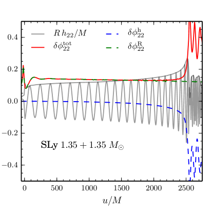
Figure 30: Error budget for the waveform phase computed from the dataset of Fig. 29.

Beside truncation and finite radius uncertainties, BNS NR waveforms can be significantly affected by systematic uncertainties related to the numerical treatment of hydrodynamics Bernuzzi et al. (2012a); Radice et al. (2014a, b). Here, we show that our analysis is not affected by such systematics. We consider additional simulations with the independent code THC Radice et al. (2014b, a). The THC waveforms have been produced specifically for this work with the goal of checking systematics uncertainties for the most challenging case for the analytical model, i.e. the MS1b configuration. The numerical setup for the THC runs is the same as in Radice et al. (2016), the employed resolutions are $h=(0.1,0.14,0.2,0.25)$. The THC runs use a high-order scheme and typically show second - to - third order convergence with sufficiently high grid resolutions.

BAM runs employ resolution $h=(0.097,0.1455,0.194,0.291)$. The phase errors are estimated using Richardson extrapolation. In Fig. 31 we compare such best waveforms for the two codes. The waveform agree within the estimated uncertainties.

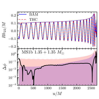
Figure 31: Systematic uncertainties in BNS numerical relativity inspiral-merger waveform. Waveforms from two independent and high-order codes are compared.

Appendix E TEOBResumS implementation details

An implementation of TEOBResumS in C/C++ is publicly available at

https://bitbucket.org/account/user/eob_ihes/projects/EOB

together with some of original TEOBResum codes developed in Matlab. The inference results on GW150914 data of Sec. V and the match results of Sec. VI are obtained with this code. An optimized implementation into the LALSuite library is currently in progress.

E.1 General considerations

The C/C++ implementation is straightforward. Main specific choices are

1. The equation of motion are written analytically and not using finite-difference derivatives of the Hamiltonian [Note this was an “optimization” of SEOBNRv2 as introduced in Devine et al. (2016)].

2. We use an eight-order adaptive-timestep Runge-Kutta order ODE solver as implemented in the GSL library.

3. After the ODE solver has completed, both the solution of the Hamilton’s equations as well as the waveform is sparsely and unevenly sampled in time (unless uniform timestep is requested). Since the waveform will eventually need to be Fourier transformed, it has to be uniformly sampled. We do it using cubic spline interpolant built within the GSL library. We note that, for our convenience, we interpolate on the evenly-spaced grid both the dynamics, that is the vector $(t,r,\varphi,p_{r_{*}},p_{\varphi})$, and the multipolar waveform.

We find that for long BNS waveforms starting at $10-20$ Hz, the computational cost of the interpolation is almost as expensive as the solution of the ODE system. Typical running times for BNS are of the order of 3.5 sec from 20Hz using a time sampling of $4096$ Hz (see Table 6 below). Such performance is not yet competitive with SEOBNRv2_opt of Ref. Devine et al. (2016) and thus cannot be directly used in parameter estimation codes for long-inspiral signals (while it is sufficiently efficient for short-inspiral ones like GW150914, as we showed in Sec. V). This is not surprising, since no actual effort towards true optimization was done at the moment and several unnecessarily repeated operations are still present. As an example of possible optimization, we discuss below an alternative implementation of the phase of the tail factor entering the resummed EOB waveform Damour et al. (2009).

E.2 Effective representation of the tail factor

This section describes the implementation of a specific term of the multipolar waveform, the tail factor. We saw in the main text that the circularized EOB multipolar waveform Damour et al. (2009) is written in the following factorized form

$$h_{\ell m}=h_{\ell m}^{\rm Newt}\hat{S}_{\rm eff}^{(\epsilon)}\hat{h}_{\ell m}^{\text{tail}}f_{\ell m}$$ (65)

where $h_{\ell m}^{\rm Newt}$ is the Newtonian prefactor, $\hat{S}_{\rm eff}^{(\epsilon)}$ is the effective source, $\epsilon$ is the parity of $\ell+m$, $f_{\ell m}$ is the residual amplitude correction and $\hat{h}_{\ell m}^{\rm tail}$ is the tail factor. The $f_{\ell m}$’s are given as Taylor series with $log$ functions appearing, so that they are one of the most expensive part of the computation. The tail factor $\hat{h}_{\ell m}^{\text{tail}}$ of the waveform is given by

$$\hat{h}_{\ell m}^{\text{tail}}(y)=T_{\ell m}(y)e^{i\delta_{\ell m}(y)}$$ (66)

with

$$T_{\ell m}(y)=\frac{\Gamma(\ell+1-2i\hat{\hat{k}})}{\Gamma(\ell+1)}e^{(\pi+2\ln(2kr_{0})i)\hat{\hat{k}}}\,,$$ (67)

where

$$k =m\Omega,$$ (68)

$$\hat{\hat{k}} =mGH_{\text{EOB}}\Omega,$$ (69)

with $r_{0}=2GM/\sqrt{e}$ and $y=(GH_{\text{EOB}}\Omega)^{2/3}$. Evaluating the full $T_{\ell m}$ as a complex number is computationally expensive as the $\Gamma$ functions need to be evaluated separately for each multipole.

To ease and speedup the implementation of those parts of the code where the $\Gamma$ functions appear, it was chosen to work separately with its argument and modulus, since only this latter is used for the computation of the GW flux that drives the dynamics. The squared modulus of the tail function, for each multipole, can be written as

$$|T_{\ell m}(y)|^{2}=\frac{1}{(\ell!)^{2}}\frac{4\pi\hat{\hat{k}}}{1-e^{-4\pi\hat{\hat{k}}}}\prod^{\ell}_{s=1}\left(s^{2}+(2\hat{\hat{k}})^{2}\right)\ ,$$ (70)

and it can be thus computed via such simple formula.

Special routines for the $\Gamma$ function are needed only for the phase of the tail term, for which a simple formula like the one above does not exists. In fact, the TEOBResumS C/C++ code uses instead the Lanczos approximation to the complex $\Gamma$ function implemented in the GSL.

As an alternative, it is possible to construct a fast and effective representation of the phase of $\Gamma$ as follows. One starts from the following representation of the argument

$$\arg\left[\Gamma(x+iy)\right]=y\psi(x)+\sum_{n=0}^{\infty}\left[\frac{y}{x+n}-\arctan\frac{y}{x+n}\right]\,,$$ (71)

where $\psi(x)\equiv\Gamma^{\prime}/\Gamma$ is the digamma function and the prime indicates the derivative with respect to $x$. In Eq. (67), the only complex $\Gamma$ is the one at the numerator, where $y\equiv 2\hat{\hat{k}}$, $x=\ell+1$ and we can formally write its phase in factorized form as

$$\sigma_{\ell}(\hat{\hat{k}})\equiv\arg\left[\Gamma(\ell+1-2{\rm i}\hat{\hat{k}})\right]=\sigma^{0}_{\ell}\hat{\sigma}^{\prime}_{\ell},$$ (72)

where we defined $\sigma_{0}^{\ell}\equiv-2i\hat{\hat{k}}\psi(\ell+1)$. The quantity $\sigma^{\prime}_{\ell}$ can be represented by a polynomial in $\hat{\hat{k}}$ whose coefficients are fitted to the actual function $\sigma^{\prime}_{\ell}(\hat{\hat{k}})$ evaluated on an interval large enough to include all possible frequencies spanned by the binary evolution. For each multipole up to $\ell=8$ we find that a fifth order polynomial of the form $\sigma^{\prime}_{\ell}=1+n^{\ell}_{2}\hat{\hat{k}}^{2}+\dots+n^{\ell}_{5}\hat{\hat{k}}^{5}$ is able to give an accurate representation of the function, with fractional difference typically of order $\lesssim 10^{-6}$.

Figure 32: Performance of the use of the ”speedy” implementation of the phase of the $\Gamma$ function versus the standard Lanczos implementation of the full $\Gamma$ function. The plot refers to a fiducial $1.35M_{\odot}+1.35M_{\odot}$ BNS system starting from 10 Hz with sampling rate of 16384Hz. $\Lambda^{A}_{2}=\Lambda^{B}_{2}$ varying from 1 to 1800. The use of the effective phase fit brings a non-negligible improvement to the performance of the code. The horizontal axis represents runtimes on a MacBook Pro with an Intel Core i7 (2.5GHz) and 16GB RAM

The improvement of performance brought by the effective representation of the tail phase is illustrated in Fig. 32. The plot refers to a fiducial $1.35M_{\odot}+1.35M_{\odot}$ BNS system starting from 10 Hz with sampling rate of 16384 Hz and $\Lambda^{A}_{2}=\Lambda^{B}_{2}$ varying from 1 to 1800. Note that to setup the TEOBResumS run, from the initial frequency one computes the initial separation using the Newtonian Kepler’s constraint, so that $r_{0}/M=\left(G\pi fM/c^{3}\right)^{-2/3}$. To convert from physical to dimensionless units we use the value of the solar mass in time units Damour and Taylor (1992) $T_{\odot}=GM_{\odot}/c^{3}=4.925490947\times 10^{-6}$ sec. The figure highlights that the use of the effective phase fit brings a non-negligible improvement to the performance of the code.

Table 6: Runtime performance benchmark for TEOBResumS over a set of standard configurations. All benchmarks were completed on a MacBook Pro with an Intel Core i7 (2.5GHz) and 16GB RAM. The code was compiled with the ${\rm g}{++}$ GNU compiler using O3 optimization. Typical performance for a BNS system from 10Hz is on the order of 45s and from 20Hz on the order of 6s. All benchmarks quoted are calculated by averaging over multiple waveform generation operations. Unless otherwise stated, we adopt the effective tail representation detailed in Appendix E.2.

System	EOS	$M_{A,B}[M_{\odot}]$	$\chi_{A,B}$	$\Lambda^{A,B}_{2}$	$f_{\rm min}\left(\rm{Hz}\right)$	Sample Rate $(\rm{Hz})$	Effective Tail	Benchmark, gcc (s)
BNS	SLy	$(1.35,1.35)$	$(0,0)$	$(392,392)$	$10$	$4096$	Yes	$21.76$
BNS	SLy	$(1.35,1.35)$	$(0,0)$	$(392,392)$	$10$	$8192$	Yes	$41.66$
BNS	SLy	$(1.35,1.35)$	$(0,0)$	$(392,392)$	$10$	$8192$	No	$43.59$
BNS	SLy	$(1.35,1.35)$	$(0,0)$	$(392,392)$	$20$	$4096$	Yes	$3.44$
BNS	SLy	$(1.35,1.35)$	$(0,0)$	$(392,392)$	$20$	$8192$	Yes	$5.84$
BNS	MS1b	$(1.35,1.35)$	$(0.1,0.1)$	$(1531,1531)$	$10$	$8192$	Yes	$40.67$
NSBH	N/A	$(6,1.35)$	$(0.4,0)$	$(0,0)$	$10$	$4096$	Yes	$17.28$
BBH	N/A	$(10,10)$	$(0.6,0.6)$	$(0,0)$	$10$	$4096$	Yes	$2.64$
BBH	N/A	$(36,29)$	$(0.5,-0.2)$	$(0,0)$	$10$	$2048$	Yes	$0.14$
BBH	N/A	$(36,29)$	$(0.5,-0.2)$	$(0,0)$	$10$	$16384$	Yes	$0.71$

Additional information is also listed in the second and third rows of Table 6, where one evaluates the impact of the effective representation of the tail on a specific BNS case. The table also lists the performance of the TEOBResumS C++ code for several standard binary configurations.

Appendix F NR-informed description of merger and postmerger

The purpose of this Appendix is to collect all the fits used by TEOBResumS to describe the $\ell=m=2$ postmerger/ringdown waveform part. We report results for the QNM quantities (i.e. frequency and damping time) as well as for all other parameters that enter the postmerger template of Ref. Damour and Nagar (2014a); Del Pozzo and Nagar (2017); Nagar et al. (2017).

These fits are an improvement with respect to those of Del Pozzo and Nagar (2017); Nagar et al. (2017) in that: (i) we use SXS data where the unphysical CoM drift is corrected Nagar et al. (2017) and (ii) we employ datasets that were not previously available. While the performance in the nonspinning case remains practically unchanged, the new information makes a difference when spins are considered. The fits are informed by the 135 SXS waveforms, 5 BAM waveforms ($q=18$) and test-particle data. All fits depend on the symmetric mass ratio $\nu$ and on a spin variable that is a suitable combination of the individual spins of the two objects. The fits are built using a hierarchical approach: (i) one first obtains results for the nonspinning sector using all available nonspinning waveforms; (ii) then, the $\nu=1/4$ behavior is determined with one-dimensional fits relying on the SXS $q=1$ waveforms; (iii) finally, all remaining data is used to determine the rest of the coefficients.

F.1 Postmerger and ringdown

Let us start by discussing the new fits of the parameters $(A_{22}^{\rm mrg},\omega_{22}^{\rm mrg},c_{3}^{\phi},c_{4}^{\phi},c_{3}^{A},\omega_{1}^{22},\alpha_{1}^{22},\alpha_{21}^{22})$ entering the postmerger template as defined below. Following Ref. Del Pozzo and Nagar (2017), the QNM-rescaled ringdown waveform is defined as $\bar{h}(\tau)\equiv e^{\sigma_{1}^{22}\tau+i\phi_{0}}h_{22}(\tau)/\nu$, where $\tau=(t-t_{\rm mrg})/M_{\rm BH}$, $\sigma_{1}^{22}\equiv\alpha_{1}^{22}+i\omega_{1}^{22}$ is the (dimensionless, $M_{\rm BH}$ rescaled) complex frequency of the fundamental (positive frequency, $\omega_{1}>0$) QNM of the $\ell=m=2$ mode and $\phi_{0}$ the phase at merger. The function $\bar{h}(\tau)$ is decomposed into phase and amplitude as

$$\bar{h}(\tau)=\hat{A}_{\bar{h}}(\tau)e^{i\phi_{\bar{h}}(\tau)}.$$ (73)

The amplitude and phase are fitted using the following ansätze

$$\hat{A}_{\bar{h}}(\tau)= c_{1}^{A}\tanh\left(c_{2}^{A}\tau+c_{3}^{A}\right)+c_{4}^{A},$$ (74)

$$\phi_{\bar{h}}(\tau)= -c_{1}^{\phi}\mathrm{ln}\left(\frac{1+c_{3}^{\phi}e^{-c_{2}^{\phi}\tau}+c_{4}^{\phi}e^{-2c_{2}^{\phi}\tau}}{1+c_{3}^{\phi}+c_{4}^{\phi}}\right).$$ (75)

Following Ref. Damour and Nagar (2014a), only three of the eight coefficients $(c_{3}^{A},c_{3}^{\phi},c_{4}^{\phi})$ are independent and need to be fitted, while the others are related to these three via several physically motivated constraints as discussed in Damour and Nagar (2014a). In practice one has

$$c_{2}^{A}= \frac{1}{2}\alpha_{21}^{22},$$ (76)

$$c_{4}^{A}= \hat{A}_{22}^{\rm mrg}-c_{1}^{A}\tanh\left(c_{3}^{A}\right),$$ (77)

$$c_{1}^{A}= \hat{A}_{22}^{\rm mrg}\alpha_{1}^{22}\frac{\cosh^{2}\left(c_{3}^{A}\right)}{c_{2}^{A}},$$ (78)

$$c_{1}^{\phi}= \Delta\omega\frac{1+c_{3}^{\phi}+c_{4}^{\phi}}{c_{2}^{\phi}\left(c_{3}^{\phi}+2c_{4}^{\phi}\right)},$$ (79)

$$c_{2}^{\phi}= \alpha_{21}^{22},$$ (80)

with $\Delta\omega\equiv\omega^{22}_{1}-M_{BH}\omega^{\rm mrg}_{22}$ and $\alpha_{21}^{22}\equiv\alpha_{2}^{22}-\alpha_{1}^{22}$.

F.1.1 Waveform amplitude and frequency at merger

The fits of the waveform amplitude and frequency at merger time, $t_{\rm mrg}\equiv t_{22}^{\rm peak}$, are obtained as follows. First, we found it useful to write the $\nu$-scaled merger amplitude as

$$\hat{A}_{22}^{\rm mrg} =\hat{A}_{\rm orb}^{\rm mrg}\hat{A}_{\rm LO}^{\rm SO}\hat{\hat{A}}_{\rm S}^{\rm mrg}.$$ (81)

In this equation, $\hat{A}^{\rm mrg}_{\rm orb}$ is the nonspinning (or orbital) contribution, $\hat{A}_{\rm LO}^{\rm SO}$ takes into account, in an heuristic way, the leading-order spin-orbit dependence (see below) and $\hat{\hat{A}}_{\rm S}^{\rm mrg}$ accounts for the remaining spin-dependence. We assume the following functional dependence for the orbital contribution

$$\hat{A}_{\rm orb}^{\rm mrg} =c_{0}^{\hat{A}^{\rm mrg}_{\rm orb}}+c^{\hat{A}^{\rm mrg}_{\rm orb}}_{1}\nu+c^{\hat{A}^{\rm mrg}_{\rm orb}}_{2}\nu^{2}.$$ (82)

Note that for this fit we do not impose the test-particle limit value (that is known Harms et al. (2014)) but we just check the consistency of the fit a posteriori. The coefficients of the fits are listed in the left column of Table 7. The spin dependence of $A_{\rm LO}^{\rm SO}$ is inspired by the analytically known spin-dependence of the $\ell=m=2$ amplitude (see e.g. Eq. (16) of Messina et al. (2018)) and we write

$$\hat{A}^{\rm SO}_{\rm LO}=1-\left(\hat{a}_{0}+\dfrac{1}{3}X_{AB}\tilde{a}_{AB}\right)x^{3/2}_{\rm mrg},$$ (83)

where $x_{\rm mrg}\equiv\left(\omega^{\rm mrg}_{22}/2\right)^{2/3}$ and $\tilde{a}_{AB}\equiv\tilde{a}_{A}-\tilde{a}_{B}$. Defining $\hat{a}_{\rm eff}\equiv\hat{a}_{0}+X_{AB}\tilde{a}_{AB}/3$, the residual spin-dependence is fitted with a rational function

$$\hat{\hat{A}}_{\rm S}^{\rm mrg}=\frac{1-n^{\hat{\hat{A}}}(\nu)\hat{a}_{\rm eff}}{1-d^{\hat{\hat{A}}}(\nu)\hat{a}_{\rm eff}},$$ (84)

where $(n^{\hat{\hat{A}}},d^{\hat{\hat{A}}})$ are quadratic functions of $X_{AB}$ defined as

$$n^{\hat{\hat{A}}}(\nu) \equiv n_{\nu=1/4}^{\hat{A}^{\rm mrg}_{\rm spin}}+n_{1}^{\hat{A}^{\rm mrg}_{\rm spin}}X_{AB}+n_{2}^{\hat{A}^{\rm mrg}_{\rm spin}}\left(X_{AB}\right)^{2},$$ (85)

$$d^{\hat{\hat{A}}}(\nu) \equiv d_{\nu=1/4}^{\hat{A}^{\rm mrg}_{\rm spin}}+d_{1}^{\hat{A}^{\rm mrg}_{\rm spin}}X_{AB}+d_{2}^{\hat{A}^{\rm mrg}_{\rm spin}}\left(X_{AB}\right)^{2}.$$ (86)

The coefficients are listed in the left column of Table 7.

Table 7: The left column shows the coefficients of the waveform amplitude at merger, defined in Eq. (81) – (86). The right column shows the coefficients of the waveform frequency at merger, defined in Eq. (89) – (90), relying on (85) – (86).

	$c_{0}^{\hat{A}^{\rm mrg}_{\rm orb}}$	$=$	$\;\;\;1.43842$	$c_{0}^{\omega^{\rm mrg}_{\rm orb}}$	$=$	$\;\;\;0.273813$
	$c_{1}^{\hat{A}^{\rm mrg}_{\rm orb}}$	$=$	$\;\;\;0.100709$	$c_{1}^{\omega^{\rm mrg}_{\rm orb}}$	$=$	$\;\;\;0.223977$
	$c_{2}^{\hat{A}^{\rm mrg}_{\rm orb}}$	$=$	$\;\;\;1.82657$	$c_{2}^{\omega^{\rm mrg}_{\rm orb}}$	$=$	$\;\;\;0.481959$
	$n_{\nu=1/4}^{\hat{A}^{\rm mrg}_{\rm spin}}$	$=$	$-0.293524$	$n_{\nu=1/4}^{\omega^{\rm mrg}_{\rm spin}}$	$=$	$-0.283200$
	$d_{\nu=1/4}^{\hat{A}^{\rm mrg}_{\rm spin}}$	$=$	$-0.472871$	$d_{\nu=1/4}^{\omega^{\rm mrg}_{\rm spin}}$	$=$	$-0.696960$
	$n_{1}^{\hat{A}^{\rm mrg}_{\rm spin}}$	$=$	$\;\;\;0.176126$	$n_{1}^{\omega^{\rm mrg}_{\rm spin}}$	$=$	$\;\;\;0.1714956$
	$n_{2}^{\hat{A}^{\rm mrg}_{\rm spin}}$	$=$	$-0.0820894$	$n_{2}^{\omega^{\rm mrg}_{\rm spin}}$	$=$	$-0.24547$
	$d_{1}^{\hat{A}^{\rm mrg}_{\rm spin}}$	$=$	$\;\;\;0.20491$	$d_{1}^{\omega^{\rm mrg}_{\rm spin}}$	$=$	$\;\;\;0.1653028$
	$d_{2}^{\hat{A}^{\rm mrg}_{\rm spin}}$	$=$	$-0.150239$	$d_{2}^{\omega^{\rm mrg}_{\rm spin}}$	$=$	$-0.1520046$

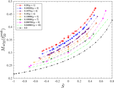
Figure 33: Uniform (or quasi-universal) behavior of the NR gravitational wave frequency at merger time $\omega_{22}^{\rm mrg}\equiv\omega_{22}(t_{22}^{\rm peak})$ for various mass ratios when plotted versus $\hat{S}=(S_{A}+S_{B})/M^{2}$. Both SXS and BAM data are shown together. It is remarkable the qualitative consistency between the test-mass limit curve (black online) and the finite mass-ratio ones.

Figure 34: Same data of Fig. 33, but plotted versus the standard effective Kerr parameter $\hat{a}_{0}=\hat{S}+\hat{S}_{*}$.

Let us turn now to discussing the merger frequency. In Fig. 33 we show the NR values of $\omega_{22}^{\rm mrg}$ versus the effective spin variable $\hat{S}\equiv(S_{A}+S_{B})/M^{2}$. It is interesting to note that, independently of the value of the two spins, there is one, smooth, curve for each mass ratio. In addition, the behavior in $\hat{S}$, that is well represented by a fourth-order polynomial in $\hat{S}$, is qualitatively the same for each configuration, including the test-mass limit (black curve in the plot). Such globally nice and simple behavior is apparent because we are using $\hat{S}$ as spin variable. In fact, had one used $\hat{a}_{0}$, that is the other natural choice of effective spin that one may consider, the curve belonging to each mass ratio becomes rather complicated, with large oscillations corresponding to those configurations where the spins are different, see Fig. 34. This is evidently the case for $q=2$ and $q=3$ data. The complete understanding of such nice property of the merger state requires a more precise study that goes beyond the purpose of this Appendix. Let us however put forward a few theoretical arguments to get an intuitive feeling of what might be going on. By assuming that $\omega_{22}^{\rm merg}\simeq 2\Omega$ (that is more true for high, positive spins), at some $u=u_{\rm mrg}$, one has

$$\omega_{22}^{\rm mrg}\simeq 2\left[\dfrac{Au_{c}^{2}p_{\varphi}^{\rm mrg}}{H_{\rm EOB}\hat{H}_{\rm eff}^{\rm orb}}+H_{\rm EOB}^{-1}\left(G_{S}\hat{S}+G_{S_{*}}\hat{S}_{*}\right)\right].$$ (87)

Since $u_{c}^{2}$ contains only even-parity powers of $\hat{a}_{0}=\hat{S}+\hat{S}_{*}$, one easily understands where the, seemingly natural, spin-dependence on $\hat{S}$ may come from. However, if the functional dependence on $\hat{S}$ is obvious for $q=1$, since $\hat{S}_{*}=\hat{S}$, it is less obvious when $q\neq 1$ because of the presence of also $\hat{S}_{*}$. In fact, Fig. 33 seems to suggest two facts: (i) the $\hat{S}_{*}$ dependence is subdominant with respect to the $\hat{S}$ one and (ii) in Eq. (87) one has to worry at most of terms quartic in $\hat{S}$, that only originate from the pure orbital part of the frequency because of $p_{\varphi}^{\rm mrg}$ and $u_{c}^{2}$. The fourth-order spin dependence is, a priori, not that surprising, because, since $u_{c}^{2}=u^{2}/(1+u^{2}(\hat{a}_{0}^{2}+2u)+\delta\hat{a}^{2}u^{2})$, it is the first correction to the leading-order spin-spin term coming from the expansion of $u_{c}^{2}$ and it is there already for a test-particle orbiting a Kerr black hole. By contrast, there is a priori no reason why $\hat{S}$ should be more important than $\hat{S}_{*}$. To get some intuition of why it is so, working in the circular approximation, we can take $u^{\rm mrg}=1/3$ as a “fiducial” merger of a binary with $q=2$, and expand Eq. (87) in both $u$ and the spins. One then verifies that the spin dependence of the quantity $u_{c}^{2}/u^{2}p_{\varphi}(u)$ at $u=u^{\rm mrg}$ is such that the coefficients of the highest powers of $\hat{S}_{*}$ (e.g. $\hat{S}_{*}^{4}$, $\hat{S}_{*}^{3}$) are numerically smaller than the corresponding ones for $\hat{S}$. By contrast, this does not happen for $(\hat{S}^{2},\hat{S}_{*}^{2})$, which indicates that the lack of symmetry between $(\hat{S},\hat{S}_{*})$ seen in Fig. 33 may just crucially stem from NLO (and higher) spin-spin effects. These facts intuitively suggest (though certainly do not explain it quantitatively) what might be the origin of the simple scaling with $\hat{S}$ illustrated in Fig. 33. This will deserve a more dedicated and extensive study on its own to be fully understood. For the moment, we content ourselves of having identified the simple structure of $\omega_{22}^{\rm mrg}$ of Fig. 33 and exploit it at best to obtain its global fit. To do so, we again assume a template in factorized form as

$$\omega_{22}^{\rm mrg}=\omega_{\rm orb}^{\rm mrg}\left(\nu\right)\omega_{\rm S}^{\rm mrg}\left(\hat{S},X_{AB}\right),$$ (88)

where the orbital factor $\omega_{\rm orb}^{\rm mrg}$ is fitted with a quadratic function in $\nu$,

$$\omega_{\rm orb}^{\rm mrg}\left(\nu\right)=c_{0}^{\omega^{\rm mrg}_{\rm orb}}+c_{1}^{\omega^{\rm mrg}_{\rm orb}}\nu+c_{2}^{\omega^{\rm mrg}_{\rm orb}}\nu^{2}.$$ (89)

The functional form of $\omega_{\rm S}^{\rm mrg}$ is identical to $\hat{\hat{A}}_{\rm S}^{\rm mrg}$ (Eq. (84)), though one is using now $\hat{S}$ as spin variable so that

$$\omega_{\rm S}^{\rm mrg}=\frac{1-n^{\omega}(\nu)\hat{S}}{1-d^{\omega}(\nu)\hat{S}}$$ (90)

where the functions $(n^{\omega},d^{\omega})$ have the same functional form as stated previously in equations (85) – (86). Coefficients of both the nonspinning and spinning parts of the fits are shown in the right column of Table 7. We found the use of the spin variable $\hat{S}$ simplified the fitting of the waveform frequency at merger. The precise analytical reason behind such simple spin dependence is currently not deeply understood. The estimate its performance, the result of the fit was compared with the full set of data available. The fractional differences are displayed in Fig. 35. The largest differences are found for $(8,0.8,0)$ and $(8,0.85,0.85)$. Since the corresponding frequency values seem to be slightly inconsistent with the expected $q=8$ trend of the frequency (see the magenta line in Fig. 33) we have conservatively preferred not to use them in the global fit.

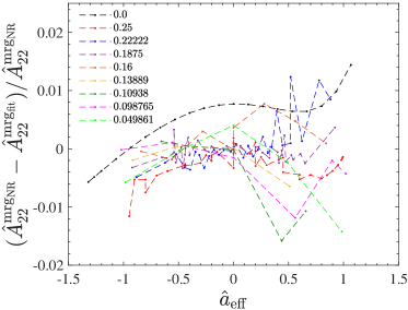
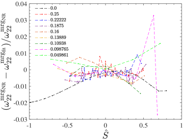
Figure 35: Evaluating the performance of the global fit of the merger amplitude given in Table 7.

F.1.2 Fits of the QNMs parameter of the final black hole

Table 8: Coefficients of the fits of the fundamental QNM frequency and inverse damping time of the final remnant $(\omega_{1},\alpha_{1})$ as well as the difference $\alpha_{21}=\alpha_{2}-\alpha_{1}$ of the inverse damping times of the first two modes. See Eq. (91) for definitions.

		$\;\;\;Y=\omega^{22}_{1}$	$\;\;\;Y=\alpha^{22}_{1}$	$\;\;\;Y=\alpha^{22}_{21}$
	$Y_{0}$	$\;\;\;0.373672$	$\;\;\;0.0889623$	$\;\;\;0.184953$
	$b_{1}^{Y}$	$-1.74085$	$-1.82261$	$-1.41681$
	$b_{2}^{Y}$	$\;\;\;0.808214$	$\;\;\;0.701584$	$-0.0593166$
	$b_{3}^{Y}$	$-0.0598838$	$\;\;\;0.121126$	$\;\;\;0.476420$
	$c_{1}^{Y}$	$-2.07641$	$-1.80020$	$-1.35955$
	$c_{2}^{Y}$	$\;\;\;1.31524$	$\;\;\;0.720117$	$-0.0763529$
	$c_{3}^{Y}$	$-0.235896$	$\;\;\;0.0811633$	$\;\;\;0.438558$

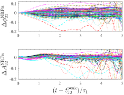
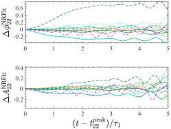
Figure 36: Left panel: The $\ell=m=2$ phasing and amplitude performance for nonspinning waveforms. Middle panel: the phasing and amplitude performance for all spinning SXS waveforms. Right panel: BAM waveforms. Top row: Phase error $\Delta\phi_{22}^{\rm NRFit}\equiv\phi^{\rm NR}_{22}-\phi^{\rm fit}_{22}$. Bottom row: Fractional amplitude difference $\Delta A^{\rm NRFit}_{22}\equiv(A^{\rm NR}_{22}-A^{\rm fit}_{22})/A^{\rm NR}_{22}$. The time is given in units of $\tau_{1}\equiv M_{\rm BH}/\alpha_{1}$.

The fits of $Y=\left\{\omega_{1}^{22},\alpha_{1}^{22},\alpha_{2}^{22}\right\}$ presented here were informed using data obtained using publicly available tables of Berti et al. Berti et al. (2006, 2009). The fits are done versus the dimensionless spin parameter $\chi_{\rm BH}\equiv J_{\rm BH}/M_{\rm BH}^{2}$ of the final black hole. $\chi_{\rm BH}$ is computed for a given set of initial conditions with the fits of Jimenez-Forteza et al. Jiménez-Forteza et al. (2017). The three parameters are fitted with rational functions after the $\chi_{\rm BH}=0$ limit was factorized

$$Y\left(\hat{a}_{f}\right)=Y_{0}\,\frac{1+b_{1}^{Y}\chi_{\rm BH}+b_{2}^{Y}\chi_{\rm BH}^{2}+b_{3}^{Y}\chi_{\rm BH}^{3}}{1+c_{1}^{Y}\chi_{\rm BH}+c_{2}^{Y}\chi_{\rm BH}^{2}+c_{3}^{Y}\chi_{\rm BH}^{3}},$$ (91)

The fitted coefficients are listed in Table 8.

F.1.3 Fits of the additional parameters

The three parameters $Y_{\rm orb}=\left\{c_{3}^{A},c_{3}^{\phi},c_{4}^{\phi}\right\}$ are first obtained by fitting each QNM-rescaled ringdown NR waveform on a time interval of length $4\tau_{1}$ after the amplitude peak, using the functional form of Eq. (74) for the QNM-rescaled amplitude, and of Eq. (75) for the QNM-rescaled phase. The result of this primary fit, done for each NR dataset considered in the main text, is then globally fitted using the following functional form

$$Y(\nu;\,\hat{S})=b^{Y}_{0}(\nu)+ b^{Y}_{1}\left(X_{AB}\right)\hat{S}+b^{Y}_{2}\left(X_{AB}\right)\hat{S}^{2}$$

$$+b^{Y}_{3}\left(X_{AB}\right)\hat{S}^{3}+b^{Y}_{4}\left(X_{AB}\right)\hat{S}^{4}.$$ (92)

The coefficients of the fit are listed in Table 9. Note that the fit of $Y=c_{3}^{A}$ is done using $\hat{a}_{\rm eff}$ instead of $\hat{S}$. To demonstrate the accuracy of the fits, Fig. 36 shows the direct comparison of the globally interpolating fits with the available NR information. The comparison is done through the difference of the waveform phase and the fractional amplitude difference. Note that two BAM waveforms show a strong dephasing. These are $(8,0.8,0)$ (light blue, solid) and $(8,0.85,0.85)$ (green, dashed), and is due to the error of the merger frequency. As mentioned above, we leave it to future work to resolve these differences.

Table 9: The fitted coefficients of $\left\{c_{3}^{A},c_{3}^{\phi},c_{4}^{\phi}\right\}$ as defined in Eq. (F.1.3).

	$Y=c_{3}^{A}$				$Y=c_{3}^{\phi}$				$Y=c_{4}^{\phi}$
	$b^{c_{3}^{A}}_{0}(\nu)$	$=$	$-0.561584$	$+0.829868\nu$	$b^{c_{3}^{\phi}}_{0}(\nu)$	$=$	$\;\;\;3.88838$	$+0.455847\nu$	$b^{c_{4}^{\phi}}_{0}(\nu)$	$=$	$1.49969$	$+2.08223\nu$
	$b^{c_{3}^{A}}_{1}(X_{AB})$	$=$	$-0.199494$	$+0.0169543X_{AB}$	$b^{c_{3}^{\phi}}_{1}(X_{AB})$	$=$	$\;\;\;5.11992$	$-0.924642X_{AB}$	$b^{c_{4}^{\phi}}_{1}(X_{AB})$	$=$	$8.26248$	$-0.899952X_{AB}$
	$b^{c_{3}^{A}}_{2}(X_{AB})$	$=$	$\;\;\;0.0227344$	$-0.0799343X_{AB}$	$b^{c_{3}^{\phi}}_{2}(X_{AB})$	$=$	$\;\;\;10.29692$	$-3.618048X_{AB}$	$b^{c_{4}^{\phi}}_{2}(X_{AB})$	$=$	$14.27808$	$-3.923652X_{AB}$
	$b^{c_{3}^{A}}_{3}(X_{AB})$	$=$	$\;\;\;0.0907477$	$-0.115928X_{AB}$	$b^{c_{3}^{\phi}}_{3}(X_{AB})$	$=$	$-4.041224$	$+3.501976X_{AB}$	$b^{c_{4}^{\phi}}_{3}(X_{AB})$	$=$	$0$
	$b^{c_{3}^{A}}_{4}(X_{AB})$	$=$	$0$		$b^{c_{3}^{\phi}}_{4}(X_{AB})$	$=$	$-32.92144$	$+29.24000X_{AB}$	$b^{c_{4}^{\phi}}_{4}(X_{AB})$	$=$	$0$

F.2 Fits of the NQC point

In this Section we present fits of the values of the NR waveform taken at the point $t_{\rm NQC}\equiv t_{\rm mrg}+2M$. On each SXS NR data set one measures the quantities $\left\{\hat{A}_{22}^{\rm NQC},\dot{\hat{A}}_{22}^{\rm NQC},\omega_{22}^{\rm NQC},\dot{\omega}_{22}^{\rm NQC}\right\}$ that are then properly fitted. These are then used to determine the NQC parameters defined in Sec. II.1. Note that the results of this Section refer to the Regge-Wheeler normalized strain waveform $\hat{\Psi}_{22}\equiv\hat{h}_{22}/\sqrt{24}$ already used in the main text. With a slight abuse of notation, we will refer here to the amplitude (and time derivative) of this quantity at $t_{\rm NQC}$ as $(\hat{A}^{\rm NQC},\dot{\hat{A}}^{\rm NQC})$ where $\hat{A}^{\rm NQC}\equiv\left|\Psi_{22}(t_{\rm NQC})\right|$.

Table 10: Coefficients of the NQC extraction points defined in Eqs. (93)-(104). From left to right the columns show $\left\{\hat{A}_{22}^{\rm NQC},\dot{\hat{A}}_{22}^{\rm NQC},\omega_{22}^{\rm NQC},\dot{\omega}_{22}^{\rm NQC}\right\}$.

$\hat{A}^{\rm NQC}_{22}$

$\dot{A}^{\rm NQC}_{22}/\nu$

$\omega^{\rm NQC}_{22}$

$\dot{\omega}^{\rm NQC}_{22}$

$c_{0}^{\hat{A}^{\rm NQC}_{\rm orb}}$

$=$

$\;\;\;0.294888$

$N_{0}^{\dot{A}^{\rm NQC}_{\rm orb}}$

$=$

$-0.00421428$

$c_{0}^{\omega^{\rm NQC}_{\rm orb}}$

$=$

$\;\;\;0.286399$

$N_{0}^{\dot{\omega}^{\rm NQC}_{\rm orb}}$

$=$

$\;\;\;0.00649349$

$c_{1}^{\hat{A}^{\rm NQC}_{\rm orb}}$

$=$

$-0.0427442$

$N_{1}^{\dot{A}^{\rm NQC}_{\rm orb}}$

$=$

$-0.0847947$

$c_{1}^{\omega^{\rm NQC}_{\rm orb}}$

$=$

$\;\;\;0.251240$

$N_{1}^{\dot{\omega}^{\rm NQC}_{\rm orb}}$

$=$

$\;\;\;0.00452138$

$c_{2}^{\hat{A}^{\rm NQC}_{\rm orb}}$

$=$

$\;\;\;0.816756$

$D_{1}^{\dot{A}^{\rm NQC}_{\rm orb}}$

$=$

$\;\,16.1559$

$c_{2}^{\omega^{\rm NQC}_{\rm orb}}$

$=$

$\;\;\;0.542717$

$D_{1}^{\dot{\omega}^{\rm NQC}_{\rm orb}}$

$=$

$-1.44664$

$c_{3}^{\hat{A}^{\rm NQC}_{\rm orb}}$

$=$

$-0.986204$

$n_{1/4}^{\hat{A}^{\rm NQC}_{\rm spin}}$

$=$

$-0.275052$

$n_{1/4}^{\dot{A}^{\rm NQC}_{\rm spin}}$

$=$

$\;\;\;0.00374616$

$n_{1/4}^{\omega^{\rm NQC}_{\rm spin}}$

$=$

$-0.292192$

$a_{1/4}^{\dot{\omega}^{\rm NQC}_{\rm spin}}$

$=$

$\;\;\;0.1209112$

$d_{1/4}^{\hat{A}^{\rm NQC}_{\rm spin}}$

$=$

$-0.469378$

$d_{1/4}^{\dot{A}^{\rm NQC}_{\rm spin}}$

$=$

$\;\;\;0.0636083$

$d_{1/4}^{\omega^{\rm NQC}_{\rm spin}}$

$=$

$-0.686036$

$b_{1/4}^{\dot{\omega}^{\rm NQC}_{\rm spin}}$

$=$

$-0.1198332$

$n_{1}^{\hat{A}^{\rm NQC}_{\rm spin}}$

$=$

$\;\;\;0.143066$

$n_{1}^{\dot{A}^{\rm NQC}_{\rm spin}}$

$=$

$\;\;\;0.00129393$

$n_{1}^{\omega^{\rm NQC}_{\rm spin}}$

$=$

$\;\;\;0.1996112$

$a_{1}^{\dot{\omega}^{\rm NQC}_{\rm spin}}$

$=$

$\;\;\;0.142343$

$n_{2}^{\hat{A}^{\rm NQC}_{\rm spin}}$

$=$

$-0.0425947$

$n_{2}^{\dot{A}^{\rm NQC}_{\rm spin}}$

$=$

$-0.00239069$

$n_{2}^{\omega^{\rm NQC}_{\rm spin}}$

$=$

$-0.236196$

$a_{2}^{\dot{\omega}^{\rm NQC}_{\rm spin}}$

$=$

$-0.1001772$

$d_{1}^{\hat{A}^{\rm NQC}_{\rm spin}}$

$=$

$\;\;\;0.176955$

$d_{1}^{\dot{A}^{\rm NQC}_{\rm spin}}$

$=$

$-0.0534209$

$d_{1}^{\omega^{\rm NQC}_{\rm spin}}$

$=$

$\;\;\;0.1843102$

$b_{1}^{\dot{\omega}^{\rm NQC}_{\rm spin}}$

$=$

$\;\;\;0.1844956$

$d_{2}^{\hat{A}^{\rm NQC}_{\rm spin}}$

$=$

$-0.111902$

$d_{2}^{\dot{A}^{\rm NQC}_{\rm spin}}$

$=$

$-0.186101$

$d_{2}^{\omega^{\rm NQC}_{\rm spin}}$

$=$

$-0.148057$

$b_{2}^{\dot{\omega}^{\rm NQC}_{\rm spin}}$

$=$

$-0.0612272$

$\hat{A}_{22}^{\rm NQC}$ is fitted similarly to the amplitude at merger by factoring it as

$$\hat{A}_{22}^{\rm NQC} =\hat{A}_{\rm orb}^{\rm NQC}\hat{A}_{\rm LO}^{\rm SO}\hat{\hat{A}}_{\rm S}^{\rm NQC},$$ (93)

with $\hat{A}_{\rm LO}^{\rm SO}$ similar to Eq. (83), however evaluated using $x_{\rm NQC}\equiv\left(\omega^{\rm NQC}_{22}/2\right)^{2/3}$. The nonspinning (orbital) contribution $\hat{A}_{\rm orb}^{\rm NQC}$ is fitted with

$$\hat{A}_{\rm orb}^{\rm NQC} =c_{3}^{\hat{A}^{\rm NQC}_{\rm orb}}\nu^{3}+c_{2}^{\hat{A}^{\rm NQC}_{\rm orb}}\nu^{2}+c_{1}^{\hat{A}^{\rm NQC}_{\rm orb}}\nu+c_{0}^{\hat{A}^{\rm NQC}_{\rm orb}}.$$ (94)

The residual spin dependence is represented as

$$\hat{\hat{A}}_{\rm S}^{\rm NQC}=\frac{1-n^{\rm NQC}_{S}\hat{a}_{\rm eff}}{1-d^{\rm NQC}_{S}\hat{a}_{\rm eff}}.$$ (95)

where $(n^{\rm NQC}_{S},d^{\rm NQC}_{S})$ are both second-order polynomial in $X_{AB}$ as defined in Eq. (85) – (86). All coefficients are listed in the first column of Table 10.

To fit the time derivative of the amplitude at $t_{\rm NQC}$ we found it useful to assume the following behavior

$$\dot{\hat{A}}_{22}^{\rm NQC} =\omega_{22}^{\rm NQC}\left[\dot{A}_{\rm orb}^{\rm NQC}\left(\nu\right)+\dot{A}_{S}^{\rm NQC}\left(\hat{a}_{\rm eff},X_{12}\right)\right].$$ (96)

The nonspinning contribution is fitted using the following rational function

$$\dot{A}_{\rm orb}^{\rm NQC}\left(\nu\right)=-\frac{N_{0}^{\dot{A}^{\rm NQC}_{\rm orb}}+N_{1}^{\dot{A}^{\rm NQC}_{\rm orb}}\nu}{1+D^{\dot{A}^{\rm NQC}_{\rm orb}}_{1}\nu}.$$ (97)

The spin-dependence is similarly fitted with a rational function of the form

$$\dot{A}_{S}^{\rm NQC}=\frac{n^{\dot{A}_{\rm NQC}}\hat{a}_{\rm eff}}{1+d^{\dot{A}_{\rm NQC}}\hat{a}_{\rm eff}},$$ (98)

where the $\nu$ dependence is encoded in the functions $({n^{\dot{A}_{\rm NQC}},d^{\dot{A}_{\rm NQC}}})$ as second-order polynomials in $X_{AB}$ as defined in Eq. (85) – (86). The explicit values of the coefficients are listed in the second column of Table 10.

We now turn our attention to the NQC frequency. We again consider a factorization as

$$M\omega_{22}^{\rm NQC}\left(\nu;\hat{S}\right) =M\omega_{\rm orb}^{\rm NQC}\left(\nu\right)\omega_{S}^{\rm NQC}\left(\hat{S},X_{AB}\right),$$ (99)

in which the nonspinning contribution is given by

$$M\omega_{\rm orb}^{\rm NQC}\left(\nu\right)=c_{0}^{\omega^{\rm NQC}_{\rm orb}}+c_{1}^{\omega^{\rm NQC}_{\rm orb}}\nu+c_{2}^{\omega^{\rm NQC}_{\rm orb}}\nu^{2}.$$ (100)

The spin factor is represented with the usual rational function

$$\omega_{S}^{\rm NQC}=\frac{1-n^{\omega^{\rm NQC}}(\nu)\hat{S}}{1-d^{\omega^{\rm NQC}}(\nu)\hat{S}},$$ (101)

where the functions $(n^{\omega^{\rm NQC}},d^{\omega^{\rm NQC}})$ are, as for the amplitude, quadratic functions of $X_{AB}$, as defined in Eq. (85) – (86). The coefficients are listed in the third column of Table 10.

The time derivative of the frequency is fitted from the following factorized ansatz

$$\dot{\omega}_{22}^{\rm NQC} =\dot{\omega}_{\rm orb}^{\rm NQC}\left(\nu\right)\dot{\omega}_{S}^{\rm NQC}\left(\hat{S},X_{AB}\right),$$ (102)

where the nonspinning part is

$$\dot{\omega}_{\rm orb}^{\rm NQC}\left(\nu\right)=\frac{N_{0}^{\dot{\omega}^{\rm NQC}_{\rm orb}}+N_{1}^{\dot{\omega}^{\rm NQC}_{\rm orb}}\nu}{1+D_{1}^{\dot{\omega}^{\rm NQC}_{\rm orb}}\nu}.$$ (103)

Finally, the spin-dependent correction is fitted with a quadratic polynomial in $\hat{S}$ as

$$\dot{\omega}_{S}^{\rm NQC}\left(\hat{S};\,X_{AB}\right)=1+a_{\dot{\omega}^{\rm NQC}}\left(\nu\right)\hat{S}+b_{\dot{\omega}^{\rm NQC}}\left(\nu\right)\hat{S}^{2},$$ (104)

where the coefficients $(a_{\dot{\omega}^{\rm NQC}},b_{\dot{\omega}^{\rm NQC}})$ are represented, as above, with quadratic functions of $X_{AB}$. The corresponding coefficients are listed in the fourth column of Table 10.

References

- Abbott et al. (2016a) B. P. Abbott et al. (Virgo, LIGO Scientific), Phys. Rev. Lett. 116, 061102 (2016a), arXiv:1602.03837 [gr-qc] .
- Abbott et al. (2016b) B. P. Abbott et al. (Virgo, LIGO Scientific), Phys. Rev. Lett. 116, 241103 (2016b), arXiv:1606.04855 [gr-qc] .
- Abbott et al. (2017a) B. P. Abbott et al. (VIRGO, LIGO Scientific), Phys. Rev. Lett. 118, 221101 (2017a), arXiv:1706.01812 [gr-qc] .
- Abbott et al. (2017b) B. P. Abbott et al. (Virgo, LIGO Scientific), Phys. Rev. Lett. 119, 161101 (2017b), arXiv:1710.05832 [gr-qc] .
- Buonanno and Damour (1999) A. Buonanno and T. Damour, Phys. Rev. D59, 084006 (1999), arXiv:gr-qc/9811091 .
- Buonanno and Damour (2000) A. Buonanno and T. Damour, Phys. Rev. D62, 064015 (2000), arXiv:gr-qc/0001013 .
- Damour (2001) T. Damour, Phys. Rev. D64, 124013 (2001), arXiv:gr-qc/0103018 .
- Damour et al. (2000) T. Damour, P. Jaranowski, and G. Schaefer, Phys. Rev. D62, 084011 (2000), arXiv:gr-qc/0005034 [gr-qc] .
- Bohé et al. (2017) A. Bohé et al., Phys. Rev. D95, 044028 (2017), arXiv:1611.03703 [gr-qc] .
- Nagar et al. (2017) A. Nagar, G. Riemenschneider, and G. Pratten, Phys. Rev. D96, 084045 (2017), arXiv:1703.06814 [gr-qc] .
- Cotesta et al. (2018) R. Cotesta, A. Buonanno, A. Boé, A. Taracchini, I. Hinder, and S. Ossokine, (2018), arXiv:1803.10701 [gr-qc] .
- Dietrich and Hinderer (2017) T. Dietrich and T. Hinderer, Phys. Rev. D95, 124006 (2017), arXiv:1702.02053 [gr-qc] .
- Damour and Nagar (2014a) T. Damour and A. Nagar, Phys.Rev. D90, 024054 (2014a), arXiv:1406.0401 [gr-qc] .
- (14) LIGO Scientific Collaboration, .
- Babak et al. (2017) S. Babak, A. Taracchini, and A. Buonanno, Phys. Rev. D95, 024010 (2017), arXiv:1607.05661 [gr-qc] .
- Nagar et al. (2016) A. Nagar, T. Damour, C. Reisswig, and D. Pollney, Phys. Rev. D93, 044046 (2016), arXiv:1506.08457 [gr-qc] .
- Damour and Nagar (2014b) T. Damour and A. Nagar, Phys.Rev. D90, 044018 (2014b), arXiv:1406.6913 [gr-qc] .
- (18) https://data.black-holes.org/waveforms/index.html, sXS Gravitational Waveform Database.
- Buchman et al. (2012) L. T. Buchman, H. P. Pfeiffer, M. A. Scheel, and B. Szilagyi, Phys. Rev. D86, 084033 (2012), arXiv:1206.3015 [gr-qc] .
- Chu et al. (2009) T. Chu, H. P. Pfeiffer, and M. A. Scheel, Phys. Rev. D80, 124051 (2009), arXiv:0909.1313 [gr-qc] .
- Hemberger et al. (2013) D. A. Hemberger, G. Lovelace, T. J. Loredo, L. E. Kidder, M. A. Scheel, B. Szilágyi, N. W. Taylor, and S. A. Teukolsky, Phys. Rev. D88, 064014 (2013), arXiv:1305.5991 [gr-qc] .
- Scheel et al. (2015) M. A. Scheel, M. Giesler, D. A. Hemberger, G. Lovelace, K. Kuper, M. Boyle, B. Szilágyi, and L. E. Kidder, Class. Quant. Grav. 32, 105009 (2015), arXiv:1412.1803 [gr-qc] .
- Blackman et al. (2015) J. Blackman, S. E. Field, C. R. Galley, B. Szilágyi, M. A. Scheel, M. Tiglio, and D. A. Hemberger, Phys. Rev. Lett. 115, 121102 (2015), arXiv:1502.07758 [gr-qc] .
- Lovelace et al. (2012) G. Lovelace, M. Boyle, M. A. Scheel, and B. Szilagyi, Class. Quant. Grav. 29, 045003 (2012), arXiv:1110.2229 [gr-qc] .
- Lovelace et al. (2011) G. Lovelace, M. Scheel, and B. Szilagyi, Phys.Rev. D83, 024010 (2011), arXiv:1010.2777 [gr-qc] .
- Lovelace et al. (2015) G. Lovelace et al., Class. Quant. Grav. 32, 065007 (2015), arXiv:1411.7297 [gr-qc] .
- Mroue et al. (2013) A. H. Mroue, M. A. Scheel, B. Szilagyi, H. P. Pfeiffer, M. Boyle, et al., Phys.Rev.Lett. 111, 241104 (2013), arXiv:1304.6077 [gr-qc] .
- Kumar et al. (2015) P. Kumar, K. Barkett, S. Bhagwat, N. Afshari, D. A. Brown, G. Lovelace, M. A. Scheel, and B. Szilagyi, Phys. Rev. D92, 102001 (2015), arXiv:1507.00103 [gr-qc] .
- Chu et al. (2016) T. Chu, H. Fong, P. Kumar, H. P. Pfeiffer, M. Boyle, D. A. Hemberger, L. E. Kidder, M. A. Scheel, and B. Szilagyi, Class. Quant. Grav. 33, 165001 (2016), arXiv:1512.06800 [gr-qc] .
- Bruegmann et al. (2008) B. Bruegmann, J. A. Gonzalez, M. Hannam, S. Husa, U. Sperhake, and W. Tichy, Phys. Rev. D77, 024027 (2008), arXiv:gr-qc/0610128 [gr-qc] .
- Husa et al. (2008) S. Husa, J. A. González, M. Hannam, B. Brügmann, and U. Sperhake, Class. Quant. Grav. 25, 105006 (2008), arXiv:0706.0740 [gr-qc] .
- Bernuzzi et al. (2015a) S. Bernuzzi, A. Nagar, T. Dietrich, and T. Damour, Phys.Rev.Lett. 114, 161103 (2015a), arXiv:1412.4553 [gr-qc] .
- Kiuchi et al. (2017) K. Kiuchi, K. Kawaguchi, K. Kyutoku, Y. Sekiguchi, M. Shibata, and K. Taniguchi, Phys. Rev. D96, 084060 (2017), arXiv:1708.08926 [astro-ph.HE] .
- Kawaguchi et al. (2018) K. Kawaguchi, K. Kiuchi, K. Kyutoku, Y. Sekiguchi, M. Shibata, and K. Taniguchi, Phys. Rev. D97, 044044 (2018), arXiv:1802.06518 [gr-qc] .
- Poisson (1998) E. Poisson, Phys. Rev. D57, 5287 (1998), arXiv:gr-qc/9709032 [gr-qc] .
- Dietrich et al. (2018a) T. Dietrich et al., (2018a), arXiv:1804.02235 [gr-qc] .
- Abbott et al. (2018a) B. P. Abbott et al. (Virgo, LIGO Scientific), (2018a), arXiv:1805.11579 [gr-qc] .
- Abbott et al. (2018b) B. P. Abbott et al. (Virgo, LIGO Scientific), (2018b), arXiv:1805.11581 [gr-qc] .
- Hinderer et al. (2016) T. Hinderer et al., Phys. Rev. Lett. 116, 181101 (2016), arXiv:1602.00599 [gr-qc] .
- Steinhoff et al. (2016) J. Steinhoff, T. Hinderer, A. Buonanno, and A. Taracchini, Phys. Rev. D94, 104028 (2016), arXiv:1608.01907 [gr-qc] .
- Vines and Marsat (2018) J. Vines and S. Marsat, (private communication, LIGO Document T1800028-v1, 2018).
- Maggiore (2007) M. Maggiore, Gravitational Waves. Vol. 1: Theory and Experiments, Oxford Master Series in Physics (Oxford University Press, 2007).
- Damour et al. (2016) T. Damour, P. Jaranowski, and G. Schäfer, Phys. Rev. D93, 084014 (2016), arXiv:1601.01283 [gr-qc] .
- Bernard et al. (2018) L. Bernard, L. Blanchet, G. Faye, and T. Marchand, Phys. Rev. D97, 044037 (2018), arXiv:1711.00283 [gr-qc] .
- Blanchet (2014) L. Blanchet, Living Rev. Relativity 17, 2 (2014), arXiv:1310.1528 [gr-qc] .
- Damour et al. (2008) T. Damour, P. Jaranowski, and G. Schäfer, Phys.Rev. D78, 024009 (2008), arXiv:0803.0915 [gr-qc] .
- Barausse and Buonanno (2010) E. Barausse and A. Buonanno, Phys.Rev. D81, 084024 (2010), arXiv:0912.3517 [gr-qc] .
- Damour (2010) T. Damour, Phys. Rev. D81, 024017 (2010), arXiv:0910.5533 [gr-qc] .
- Damour and Nagar (2010) T. Damour and A. Nagar, Phys. Rev. D81, 084016 (2010), arXiv:0911.5041 [gr-qc] .
- Damour (2016) T. Damour, Phys. Rev. D94, 104015 (2016), arXiv:1609.00354 [gr-qc] .
- Vines (2018) J. Vines, Class. Quant. Grav. 35, 084002 (2018), arXiv:1709.06016 [gr-qc] .
- Damour (2018) T. Damour, Phys. Rev. D97, 044038 (2018), arXiv:1710.10599 [gr-qc] .
- Hartung and Steinhoff (2011a) J. Hartung and J. Steinhoff, Phys. Rev. D83, 044008 (2011a), arXiv:1011.1179 [gr-qc] .
- Balmelli and Jetzer (2015) S. Balmelli and P. Jetzer, Phys. Rev. D91, 064011 (2015), arXiv:1502.01343 [gr-qc] .
- Nagar (2011) A. Nagar, Phys.Rev. D84, 084028 (2011), arXiv:1106.4349 [gr-qc] .
- Hartung and Steinhoff (2011b) J. Hartung and J. Steinhoff, Annalen Phys. 523, 783 (2011b), arXiv:1104.3079 [gr-qc] .
- Barausse and Buonanno (2011) E. Barausse and A. Buonanno, Phys.Rev. D84, 104027 (2011), arXiv:1107.2904 [gr-qc] .
- Damour et al. (2009) T. Damour, B. R. Iyer, and A. Nagar, Phys. Rev. D79, 064004 (2009), arXiv:0811.2069 [gr-qc] .
- Damour and Nagar (2008) T. Damour and A. Nagar, Phys. Rev. D77, 024043 (2008), arXiv:0711.2628 [gr-qc] .
- Damour et al. (2013) T. Damour, A. Nagar, and S. Bernuzzi, Phys.Rev. D87, 084035 (2013), arXiv:1212.4357 [gr-qc] .
- Nagar and Rezzolla (2005) A. Nagar and L. Rezzolla, Class. Quant. Grav. 22, R167 (2005), arXiv:gr-qc/0502064 .
- Pan et al. (2011) Y. Pan, A. Buonanno, R. Fujita, E. Racine, and H. Tagoshi, Phys.Rev. D83, 064003 (2011), arXiv:1006.0431 [gr-qc] .
- Damour and Nagar (2007) T. Damour and A. Nagar, Phys. Rev. D76, 064028 (2007), arXiv:0705.2519 [gr-qc] .
- Del Pozzo and Nagar (2017) W. Del Pozzo and A. Nagar, Phys. Rev. D95, 124034 (2017), arXiv:1606.03952 [gr-qc] .
- Boyle (2016) M. Boyle, Phys. Rev. D 93, 084031 (2016), arXiv:1509.00862 [gr-qc] .
- Harms et al. (2014) E. Harms, S. Bernuzzi, A. Nagar, and A. Zenginoglu, Class.Quant.Grav. 31, 245004 (2014), arXiv:1406.5983 [gr-qc] .
- Nagar and Shah (2016) A. Nagar and A. Shah, Phys. Rev. D94, 104017 (2016), arXiv:1606.00207 [gr-qc] .
- Messina et al. (2018) F. Messina, A. Maldarella, and A. Nagar, Phys. Rev. D97, 084016 (2018), arXiv:1801.02366 [gr-qc] .
- Jiménez-Forteza et al. (2017) X. Jiménez-Forteza, D. Keitel, S. Husa, M. Hannam, S. Khan, and M. Pürrer, Phys. Rev. D95, 064024 (2017), arXiv:1611.00332 [gr-qc] .
- Berti et al. (2006) E. Berti, V. Cardoso, and C. M. Will, Phys. Rev. D73, 064030 (2006), arXiv:gr-qc/0512160 .
- Berti et al. (2009) E. Berti, V. Cardoso, and A. O. Starinets, Class. Quant. Grav. 26, 163001 (2009), arXiv:0905.2975 [gr-qc] .
- (72) D. Shoemaker, https://dcc.ligo.org/cgi-bin/DocDB/ShowDocument?docid=2974 .
- Husa et al. (2016) S. Husa, S. Khan, M. Hannam, M. Pürrer, F. Ohme, X. Jiménez Forteza, and A. Bohé, Phys. Rev. D93, 044006 (2016), arXiv:1508.07250 [gr-qc] .
- Khan et al. (2016) S. Khan, S. Husa, M. Hannam, F. Ohme, M. Pürrer, X. Jiménez Forteza, and A. Bohé, Phys. Rev. D93, 044007 (2016), arXiv:1508.07253 [gr-qc] .
- Keitel et al. (2017) D. Keitel et al., Phys. Rev. D96, 024006 (2017), arXiv:1612.09566 [gr-qc] .
- Taracchini et al. (2014a) A. Taracchini, A. Buonanno, G. Khanna, and S. A. Hughes, Phys.Rev. D90, 084025 (2014a), arXiv:1404.1819 [gr-qc] .
- Damour (1983) T. Damour, in Gravitational Radiation, edited by N. Deruelle and T. Piran (North-Holland, Amsterdam, 1983) pp. 59–144.
- Damour et al. (1993) T. Damour, M. Soffel, and C.-m. Xu, Phys. Rev. D47, 3124 (1993).
- Racine and Flanagan (2005) E. Racine and E. E. Flanagan, Phys. Rev. D71, 044010 (2005), [Erratum: Phys. Rev.D88,no.8,089903(2013)], arXiv:gr-qc/0404101 [gr-qc] .
- Flanagan and Hinderer (2008) E. E. Flanagan and T. Hinderer, Phys.Rev. D77, 021502 (2008), arXiv:0709.1915 [astro-ph] .
- Vines et al. (2011) J. Vines, E. E. Flanagan, and T. Hinderer, Phys. Rev. D83, 084051 (2011), arXiv:1101.1673 [gr-qc] .
- Hinderer et al. (2010) T. Hinderer, B. D. Lackey, R. N. Lang, and J. S. Read, Phys. Rev. D81, 123016 (2010), arXiv:0911.3535 [astro-ph.HE] .
- Bernuzzi et al. (2014) S. Bernuzzi, A. Nagar, S. Balmelli, T. Dietrich, and M. Ujevic, Phys.Rev.Lett. 112, 201101 (2014), arXiv:1402.6244 [gr-qc] .
- Hinderer (2008) T. Hinderer, Astrophys.J. 677, 1216 (2008), arXiv:0711.2420 [astro-ph] .
- Damour and Nagar (2009) T. Damour and A. Nagar, Phys. Rev. D80, 084035 (2009), arXiv:0906.0096 [gr-qc] .
- Binnington and Poisson (2009) T. Binnington and E. Poisson, Phys. Rev. D80, 084018 (2009), arXiv:0906.1366 [gr-qc] .
- Damour and Lecian (2009) T. Damour and O. M. Lecian, Phys. Rev. D80, 044017 (2009), arXiv:0906.3003 [gr-qc] .
- Gürlebeck (2015) N. Gürlebeck, Phys. Rev. Lett. 114, 151102 (2015), arXiv:1503.03240 [gr-qc] .
- Bini and Damour (2014) D. Bini and T. Damour, Phys.Rev. D90, 124037 (2014), arXiv:1409.6933 [gr-qc] .
- Bernuzzi et al. (2015b) S. Bernuzzi, T. Dietrich, and A. Nagar, Phys. Rev. Lett. 115, 091101 (2015b), arXiv:1504.01764 [gr-qc] .
- Zappa et al. (2018) F. Zappa, S. Bernuzzi, D. Radice, A. Perego, and T. Dietrich, Phys. Rev. Lett. 120, 111101 (2018), arXiv:1712.04267 [gr-qc] .
- Del Pozzo et al. (2013) W. Del Pozzo, T. G. F. Li, M. Agathos, C. Van Den Broeck, and S. Vitale, Phys. Rev. Lett. 111, 071101 (2013), arXiv:1307.8338 [gr-qc] .
- Agathos et al. (2015) M. Agathos, J. Meidam, W. Del Pozzo, T. G. F. Li, M. Tompitak, J. Veitch, S. Vitale, and C. V. D. Broeck, Phys. Rev. D92, 023012 (2015), arXiv:1503.05405 [gr-qc] .
- Bini et al. (2012) D. Bini, T. Damour, and G. Faye, Phys.Rev. D85, 124034 (2012), arXiv:1202.3565 [gr-qc] .
- Bernuzzi et al. (2012a) S. Bernuzzi, A. Nagar, M. Thierfelder, and B. Brügmann, Phys.Rev. D86, 044030 (2012a), arXiv:1205.3403 [gr-qc] .
- Dolan et al. (2015) S. R. Dolan, P. Nolan, A. C. Ottewill, N. Warburton, and B. Wardell, Phys. Rev. D91, 023009 (2015), arXiv:1406.4890 [gr-qc] .
- Vines and Flanagan (2010) J. E. Vines and E. E. Flanagan, Phys. Rev. D88, 024046 (2010), arXiv:1009.4919 [gr-qc] .
- Damour et al. (2012) T. Damour, A. Nagar, and L. Villain, Phys.Rev. D85, 123007 (2012), arXiv:1203.4352 [gr-qc] .
- Hotokezaka et al. (2015) K. Hotokezaka, K. Kyutoku, H. Okawa, and M. Shibata, Phys. Rev. D91, 064060 (2015), arXiv:1502.03457 [gr-qc] .
- Hotokezaka et al. (2016) K. Hotokezaka, K. Kyutoku, Y.-i. Sekiguchi, and M. Shibata, Phys. Rev. D93, 064082 (2016), arXiv:1603.01286 [gr-qc] .
- Lackey et al. (2017) B. D. Lackey, S. Bernuzzi, C. R. Galley, J. Meidam, and C. Van Den Broeck, Phys. Rev. D95, 104036 (2017), arXiv:1610.04742 [gr-qc] .
- Levi and Steinhoff (2014) M. Levi and J. Steinhoff, JCAP 1412, 003 (2014), arXiv:1408.5762 [gr-qc] .
- Balmelli and Damour (2015) S. Balmelli and T. Damour, Phys. Rev. D92, 124022 (2015), arXiv:1509.08135 [gr-qc] .
- Porto and Rothstein (2008) R. A. Porto and I. Z. Rothstein, Phys. Rev. D78, 044012 (2008), [Erratum: Phys. Rev.D81,029904(2010)], arXiv:0802.0720 [gr-qc] .
- Bohé et al. (2015) A. Bohé, G. Faye, S. Marsat, and E. K. Porter, Class. Quant. Grav. 32, 195010 (2015), arXiv:1501.01529 [gr-qc] .
- Sennett et al. (2017) N. Sennett, T. Hinderer, J. Steinhoff, A. Buonanno, and S. Ossokine, Phys. Rev. D96, 024002 (2017), arXiv:1704.08651 [gr-qc] .
- Marsat and Bohé (2018) S. Marsat and A. Bohé, (private communication, 2018).
- Yagi and Yunes (2013a) K. Yagi and N. Yunes, Science 341, 365 (2013a), arXiv:1302.4499 [gr-qc] .
- Yagi and Yunes (2013b) K. Yagi and N. Yunes, Phys.Rev. D88, 023009 (2013b), arXiv:1303.1528 [gr-qc] .
- Harry and Hinderer (2018) I. Harry and T. Hinderer, Class. Quant. Grav. 35, 145010 (2018), arXiv:1801.09972 [gr-qc] .
- Tichy (2011) W. Tichy, Phys.Rev. D84, 024041 (2011), arXiv:1107.1440 [gr-qc] .
- Tichy (2012) W. Tichy, Phys. Rev. D 86, 064024 (2012), arXiv:1209.5336 [gr-qc] .
- Dietrich et al. (2015) T. Dietrich, N. Moldenhauer, N. K. Johnson-McDaniel, S. Bernuzzi, C. M. Markakis, B. Brügmann, and W. Tichy, Phys. Rev. D92, 124007 (2015), arXiv:1507.07100 [gr-qc] .
- Brügmann et al. (2008) B. Brügmann, J. A. Gonzalez, M. Hannam, S. Husa, U. Sperhake, et al., Phys.Rev. D77, 024027 (2008), arXiv:gr-qc/0610128 [gr-qc] .
- Thierfelder et al. (2011) M. Thierfelder, S. Bernuzzi, and B. Brügmann, Phys.Rev. D84, 044012 (2011), arXiv:1104.4751 [gr-qc] .
- Bernuzzi and Dietrich (2016) S. Bernuzzi and T. Dietrich, Phys. Rev. D94, 064062 (2016), arXiv:1604.07999 [gr-qc] .
- Dietrich et al. (2017a) T. Dietrich, S. Bernuzzi, and W. Tichy, Phys. Rev. D96, 121501 (2017a), arXiv:1706.02969 [gr-qc] .
- Dietrich et al. (2018b) T. Dietrich, S. Bernuzzi, B. Brügmann, and W. Tichy, in 2018 26th Euromicro International Conference on Parallel, Distributed and Network-based Processing (PDP) (2018) pp. 682–689, arXiv:1803.07965 [gr-qc] .
- Radice et al. (2014a) D. Radice, L. Rezzolla, and F. Galeazzi, Class.Quant.Grav. 31, 075012 (2014a), arXiv:1312.5004 [gr-qc] .
- Radice et al. (2014b) D. Radice, L. Rezzolla, and F. Galeazzi, Mon.Not.Roy.Astron.Soc. 437, L46 (2014b), arXiv:1306.6052 [gr-qc] .
- Baiotti et al. (2011) L. Baiotti, T. Damour, B. Giacomazzo, A. Nagar, and L. Rezzolla, Phys. Rev. D84, 024017 (2011), arXiv:1103.3874 [gr-qc] .
- Kramer and Wex (2009) M. Kramer and N. Wex, Class. Quant. Grav. 26, 073001 (2009).
- Favata (2014) M. Favata, Phys.Rev.Lett. 112, 101101 (2014), arXiv:1310.8288 [gr-qc] .
- Cho and Lee (2018) H.-S. Cho and C.-H. Lee, J. Korean Phys. Soc. 72, 1 (2018), arXiv:1708.00426 [gr-qc] .
- Dietrich et al. (2017b) T. Dietrich, S. Bernuzzi, M. Ujevic, and W. Tichy, Phys. Rev. D95, 044045 (2017b), arXiv:1611.07367 [gr-qc] .
- Damour et al. (2001) T. Damour, B. R. Iyer, and B. S. Sathyaprakash, Phys. Rev. D63, 044023 (2001), [Erratum: Phys. Rev.D72,029902(2005)], arXiv:gr-qc/0010009 [gr-qc] .
- Buonanno et al. (2009) A. Buonanno, B. Iyer, E. Ochsner, Y. Pan, and B. Sathyaprakash, Phys.Rev. D80, 084043 (2009), arXiv:0907.0700 [gr-qc] .
- Marsat (2015) S. Marsat, Class. Quant. Grav. 32, 085008 (2015), arXiv:1411.4118 [gr-qc] .
- Bernard et al. (2017) L. Bernard, L. Blanchet, A. Bohé, G. Faye, and S. Marsat, Phys. Rev. D95, 044026 (2017), arXiv:1610.07934 [gr-qc] .
- Damour et al. (2015) T. Damour, P. Jaranowski, and G. Schäfer, Phys. Rev. D91, 084024 (2015), arXiv:1502.07245 [gr-qc] .
- Damour et al. (2014) T. Damour, P. Jaranowski, and G. Schäfer, Phys. Rev. D89, 064058 (2014), arXiv:1401.4548 [gr-qc] .
- Blanchet and Damour (1988) L. Blanchet and T. Damour, Phys. Rev. D37, 1410 (1988).
- Blanchet and Damour (1992) L. Blanchet and T. Damour, Phys. Rev. D46, 4304 (1992).
- Messina and Nagar (2017) F. Messina and A. Nagar, Phys. Rev. D95, 124001 (2017), [Erratum: Phys. Rev.D96,no.4,049907(2017)], arXiv:1703.08107 [gr-qc] .
- Baiotti et al. (2010) L. Baiotti, T. Damour, B. Giacomazzo, A. Nagar, and L. Rezzolla, Phys. Rev. Lett. 105, 261101 (2010), arXiv:1009.0521 [gr-qc] .
- Abbott et al. (2016c) B. P. Abbott et al. (Virgo, LIGO Scientific), Phys. Rev. Lett. 116, 241102 (2016c), arXiv:1602.03840 [gr-qc] .
- (137) https://losc.ligo.org/about/, LIGO Open Science Center.
- (138) https://github.com/johnveitch/cpnest, Parallel nested sampling algorithm in python.
- Abbott et al. (2016d) T. D. Abbott et al. (Virgo, LIGO Scientific), Phys. Rev. X6, 041014 (2016d), arXiv:1606.01210 [gr-qc] .
- Taracchini et al. (2014b) A. Taracchini, A. Buonanno, Y. Pan, T. Hinderer, M. Boyle, et al., Phys.Rev. D89, 061502 (2014b), arXiv:1311.2544 [gr-qc] .
- Barausse et al. (2012) E. Barausse, A. Buonanno, and A. Le Tiec, Phys.Rev. D85, 064010 (2012), arXiv:1111.5610 [gr-qc] .
- Bini and Damour (2013) D. Bini and T. Damour, Phys.Rev. D87, 121501 (2013), arXiv:1305.4884 [gr-qc] .
- Healy et al. (2017) J. Healy, C. O. Lousto, and Y. Zlochower, Phys. Rev. D96, 024031 (2017), arXiv:1705.07034 [gr-qc] .
- Faye et al. (2015) G. Faye, L. Blanchet, and B. R. Iyer, Class. Quant. Grav. 32, 045016 (2015), arXiv:1409.3546 [gr-qc] .
- Buonanno et al. (2006) A. Buonanno, Y. Chen, and T. Damour, Phys. Rev. D74, 104005 (2006), arXiv:gr-qc/0508067 .
- Nagar and Gunnar (2018) A. Nagar and R. Gunnar, (in preparation, 2018).
- Nagar and Rettegno (2018) A. Nagar and P. Rettegno, (2018), arXiv:1805.03891 [gr-qc] .
- Lange et al. (2018) J. Lange, R. O’Shaughnessy, and M. Rizzo, (2018), arXiv:1805.10457 [gr-qc] .
- Hinder et al. (2018) I. Hinder, L. Kidder, H. Pfeiffer, M. Scheel, M. Boyle, D. Hemberger, G. Lovelace, and B. Szilagyi, “Binary black-hole simulation sxs:bbh:1375,” (2018).
- Bernuzzi and Nagar (2010) S. Bernuzzi and A. Nagar, Phys. Rev. D81, 084056 (2010), arXiv:1003.0597 [gr-qc] .
- Bernuzzi et al. (2012b) S. Bernuzzi, M. Thierfelder, and B. Brügmann, Phys.Rev. D85, 104030 (2012b), arXiv:1109.3611 [gr-qc] .
- Radice et al. (2016) D. Radice, S. Bernuzzi, and C. D. Ott, Phys. Rev. D94, 064011 (2016), arXiv:1603.05726 [gr-qc] .
- Devine et al. (2016) C. Devine, Z. B. Etienne, and S. T. McWilliams, Class. Quant. Grav. 33, 125025 (2016), arXiv:1601.03393 [astro-ph.HE] .
- Damour and Taylor (1992) T. Damour and J. H. Taylor, Phys. Rev. D45, 1840 (1992).