Cycle-Consistent Adversarial Learning as
Approximate Bayesian Inference

Abstract

We formalize the problem of learning inter-domain correspondences in the absence of paired data as Bayesian inference in a latent variable model (lvm), where one seeks the underlying hidden representations of entities from one domain as entities from the other domain. First, we introduce implicit latent variable models, where the prior over hidden representations can be specified flexibly as an implicit distribution. Next, we develop a new variational inference (vi) algorithm for this model based on minimization of the symmetric Kullback-Leibler (kl) divergence between a variational joint and the exact joint distribution. Lastly, we demonstrate that the state-of-the-art cycle-consistent adversarial learning (cyclegan) models can be derived as a special case within our proposed vi framework, thus establishing its connection to approximate Bayesian inference methods.

*

1 Introduction

Learning correspondences between entities from different domains is an important and challenging problem in machine learning, especially in the absence of paired data. Consider for example the task of image-to-image translation where we want to learn a mapping from an image in a source domain, such as a photograph of a natural scene, to a corresponding image in a target domain, such as the realization of such a scene in an 1860s celebrated artist’s signature impressionistic style. The shortage of ground-truth pairings from the source domain to the target domain renders standard supervised approaches infeasible, thus motivating the need for unsupervised learning approaches.

Within these unsupervised approaches, a number of recently proposed cycle-consistent adversarial learning (cyclegan)methods have achieved remarkable success in addressing this problem (Kim et al., 2017; Zhu et al., 2017). As their name suggests, these approaches are based upon two heuristics: (i) adversarial learning and (ii) cycle consistency. The former, adversarial learning (Goodfellow et al., 2014), allows images in the source domain to be translated to output images that, to an auxiliary discriminator, are indistinguishable from images in the target domain, thereby matching their distributions. However, while distribution matching is necessary, it is insufficient to guarantee one-to-one mappings between the images, as the problem is heavily under-constrained. Briefly stated, the cycle-consistency is the constraint that an image mapped to a target domain should be representable in the original domain. It is this constraint that significantly shrinks the space of possible solutions.

Beyond the empirical risk minimization framework motivated intuitively by the two conceptually simple principles mentioned above, the original cyclegan formulation lacks any further theoretical justification. This hinders (i) understanding of the distributional assumptions of all the variables of interest; (ii) how these are combined in terms of prior knowledge and observational assumptions; and (iii) whether more general methods can be used for estimating their parameters. In contrast, lvms offer a principled framework for probabilistic reasoning about random variables, their statistical properties and dependency structures, with the goal of capturing the underlying data-generation process. Besides providing sound quantification of uncertainty, a lvm allows us to disentangle our modeling assumptions from the inference machinery we use to reason about the variables in the model. Interpreting standard methods from a Bayesian perspective has contributed significantly to the understanding of these methods and to the development of new approaches. Examples of this include the seminal work on probabilistic principal component analysis (ppca) (Tipping & Bishop, 1999) and more recently, the advances in understanding Dropout (Gal & Ghahramani, 2015). Our contributions are threefold, and are summarized below.

First contribution  (§ 2). We formulate the problem of learning correspondences between domains using unpaired data from a lvm perspective, where entities in one domain are latent representations of entities in the other domain. Crucial to our approach is to consider an implicit prior over these hidden representations, i.e. a prior that is not given by a prescribed distribution such as a Gaussian, but instead, is provided via samples from an unknown process.

Second contribution  (§§ 3 and 4). We develop a new scalable variational inference algorithm for these types of models. Unlike standard vi approaches that approximate the posterior over the latent variables, we approximate the exact joint distribution over latent and observed variables with a variational joint. Furthermore, we carry out this approximation via the minimization of the symmetric kl divergence between these joints. This is in stark contrast with traditional vi approaches that minimize the forward kl divergence, as the symmetric kl divergence between the posteriors is intractable.

Third contribution  (§ 5). Finally, we show that cyclegans, as proposed by (Zhu et al., 2017; Kim et al., 2017) independently, can be recovered by applying our approximate inference algorithm in a lvm for domain correspondence with unpaired data. In this model, the prior is specified by an implicit empirical distribution and the observed variables are generated by a nonlinear function of its underlying latent variable. Intuitively, while using the symmetric kl divergence between the approximate and true joint distributions yields generative adversarial network (gan)-like objectives between the domains, different specifications of the likelihood and the approximate posterior yield the cycle-consistency part of the loss in cyclegans.

2 Implicit Latent Variable Models

Latent variable models (lvms)are an indispensable tool for uncovering the hidden representations of observed data. In a lvm, an observation ${\boldsymbol{\mathbf{x}}}$ is assumed governed by its underlying hidden variable ${\boldsymbol{\mathbf{z}}}$, which is drawn from a prior $p({\boldsymbol{\mathbf{z}}})$ and related to ${\boldsymbol{\mathbf{x}}}$ through the likelihood $p_{{\boldsymbol{\mathbf{\theta}}}}({\boldsymbol{\mathbf{x}}}\,|\,{\boldsymbol{\mathbf{z}}})$. Accordingly, the joint density of ${\boldsymbol{\mathbf{x}}}$ and ${\boldsymbol{\mathbf{z}}}$ is given by

$$p_{{\boldsymbol{\mathbf{\theta}}}}({\boldsymbol{\mathbf{x}}},{\boldsymbol{\mathbf{z}}})=p_{{\boldsymbol{\mathbf{\theta}}}}({\boldsymbol{\mathbf{x}}}\,|\,{\boldsymbol{\mathbf{z}}})p({\boldsymbol{\mathbf{z}}}).$$ (1)

Given data distribution $q^{*}({\boldsymbol{\mathbf{x}}})$ and a finite collection ${\boldsymbol{\mathbf{X}}}=\{{\boldsymbol{\mathbf{x}}}_{n}\}_{n=1}^{N}$ of observations ${\boldsymbol{\mathbf{x}}}_{n}\sim q^{*}({\boldsymbol{\mathbf{x}}})$, and the set of corresponding latent variables ${\boldsymbol{\mathbf{Z}}}=\{{\boldsymbol{\mathbf{z}}}_{n}\}_{n=1}^{N}$, the joint over all variables factorizes as,

$$p_{{\boldsymbol{\mathbf{\theta}}}}({\boldsymbol{\mathbf{X}}},{\boldsymbol{\mathbf{Z}}})=\prod_{n=1}^{N}p_{{\boldsymbol{\mathbf{\theta}}}}({\boldsymbol{\mathbf{x}}}_{n},{\boldsymbol{\mathbf{z}}}_{n}).$$ (2)

The graphical representation of this model is depicted in fig. A.2.

2.1 Prescribed Likelihood

We specify the likelihood through a mapping $\mathcal{F}_{{\boldsymbol{\mathbf{\theta}}}}$ that takes as input random noise ${\boldsymbol{\mathbf{\xi}}}$ and latent variable ${\boldsymbol{\mathbf{z}}}$,

$$\begin{split}{\boldsymbol{\mathbf{x}}}&\sim p_{{\boldsymbol{\mathbf{\theta}}}}({\boldsymbol{\mathbf{x}}}\,|\,{\boldsymbol{\mathbf{z}}})\\ \Leftrightarrow{\boldsymbol{\mathbf{x}}}&=\mathcal{F}_{{\boldsymbol{\mathbf{\theta}}}}({\boldsymbol{\mathbf{\xi}}};{\boldsymbol{\mathbf{z}}}),\quad{\boldsymbol{\mathbf{\xi}}}\sim p({\boldsymbol{\mathbf{\xi}}}).\end{split}$$ (3)

We shall restrict our attention to prescribed likelihoods, where evaluation of their density is tractable. This requires that $\mathcal{F}_{{\boldsymbol{\mathbf{\theta}}}}(\,\cdot\,;{\boldsymbol{\mathbf{z}}})$ be a diffeomorphism w.r.t. ${\boldsymbol{\mathbf{\xi}}}$ and density $p({\boldsymbol{\mathbf{\xi}}})$ be tractable. For example, when $\mathcal{F}_{{\boldsymbol{\mathbf{\theta}}}}(\,\cdot\,;{\boldsymbol{\mathbf{z}}})$ is a location-scale transform of noise ${\boldsymbol{\mathbf{\xi}}}$ and $p({\boldsymbol{\mathbf{\xi}}})$ is Gaussian, we recover a class of familiar Gaussian observation models. In appendix B, we give concrete examples of common latent variable models that can be instantiated under this definition.

2.2 Implicit Prior

In lvms, the prior is almost invariably specified as a prescribed distribution, most typically a factorized Gaussian centered at zero. Oftentimes, however, the practitioner possesses prior knowledge that simply cannot be embodied within a prescribed distribution. To address this limitation, we introduce implicit lvms, wherein the prior over latent variables is specified as an implicit distribution $p^{*}({\boldsymbol{\mathbf{z}}})$, given only by a finite collection ${\boldsymbol{\mathbf{Z}}}^{*}=\{{\boldsymbol{\mathbf{z}}}_{m}^{*}\}_{m=1}^{M}$ of its samples,

$${\boldsymbol{\mathbf{z}}}_{m}^{*}\sim p^{*}({\boldsymbol{\mathbf{z}}}).$$ (4)

This formulation offers the utmost degree of flexibility in the treatment of prior information, the difficulties of which have hindered the application of Bayesian statistics since the time of Laplace (Jaynes, 1968).

2.3 Example: Unpaired Image-to-Image Translation

Suppose we have collections of images ${\boldsymbol{\mathbf{X}}}$ and ${\boldsymbol{\mathbf{Z}}}^{*}$, which are assumed to be draws from the data distribution $q^{*}({\boldsymbol{\mathbf{x}}})$ and implicit prior distribution $p^{*}({\boldsymbol{\mathbf{z}}})$, respectively. For example, these might be photographs of natural landscapes and the paintings of Van Gogh.

The goal of unpaired image-to-image translation is to learn the correspondence between variables ${\boldsymbol{\mathbf{x}}}$ and ${\boldsymbol{\mathbf{z}}}$ by capturing the underlying generative process specified by mapping $\mathcal{F}_{{\boldsymbol{\mathbf{\theta}}}}$. This defines the likelihood $p_{{\boldsymbol{\mathbf{\theta}}}}({\boldsymbol{\mathbf{x}}}\,|\,{\boldsymbol{\mathbf{z}}})$—a conditional density of ${\boldsymbol{\mathbf{x}}}$ given ${\boldsymbol{\mathbf{z}}}$. Continuing with the above example, the problem amounts to learning parameters ${\boldsymbol{\mathbf{\theta}}}$ of the mapping such that this conditional yields photorealistic renderings of scenes portrayed in Van Gogh’s paintings. Furthermore, the resulting posterior on the latent representation $p_{{\boldsymbol{\mathbf{\theta}}}}({\boldsymbol{\mathbf{z}}}\,|\,{\boldsymbol{\mathbf{x}}})$—a conditional density of ${\boldsymbol{\mathbf{z}}}$ given ${\boldsymbol{\mathbf{x}}}$—should produce renderings of landscape scenery in Van Gogh’s iconic style.

inline]The posterior satisfies this automatically. By Bayes’ rule, its places its mass on configurations of the latent variables that explain, or generate, the observed data (photorealistic images), and configurations that match the support of the implicit prior (samples of Van Gogh paintings)

The parameters are learned maximum likelihood estimation, by marginalizing out the latent variables and maximizing the marginal likelihood

Parameter learning and inference in implicit latent variable models (ilvms) is paved with intractabilities. For moderately complicated likelihoods, the marginal likelihood $p_{{\boldsymbol{\mathbf{\theta}}}}({\boldsymbol{\mathbf{x}}})$ is intractable, making it infeasible to perform maximum likelihood estimation of ${\boldsymbol{\mathbf{\theta}}}$ and to compute the posterior exactly. Furthermore, the intractability of the prior renders most existing approximate inference methods futile. The remainder of this paper will be devoted to accurate and scalable approximate inference in ilvms.

3 Variational Inference with Implicit Priors

In this section, we describe the first component of our bipartite vi framework. In traditional vi, one specifies a family $\mathcal{Q}$ of densities over the latent variables and seeks the member $q\in\mathcal{Q}$ closest in kl divergence to the exact posterior $p_{{\boldsymbol{\mathbf{\theta}}}}({\boldsymbol{\mathbf{z}}}\,|\,{\boldsymbol{\mathbf{x}}})$ (Jordan et al., 1999; Wainwright & Jordan, 2008; Blei et al., 2017).

3.1 Prescribed Variational Posterior

We begin by describing the variational family $q\in\mathcal{Q}$. We adopt the common practice of amortizing inference using an inference network (Gershman & Goodman, 2014). Namely, instead of approximating the exact posterior $p_{{\boldsymbol{\mathbf{\theta}}}}({\boldsymbol{\mathbf{z}}}\,|\,{\boldsymbol{\mathbf{x}}}_{n})$ for each ${\boldsymbol{\mathbf{x}}}_{n}$, using a separate variational distribution $q({\boldsymbol{\mathbf{z}}};{\boldsymbol{\mathbf{\lambda}}}_{n})$ with local variational parameters ${\boldsymbol{\mathbf{\lambda}}}_{n}$, we condition on ${\boldsymbol{\mathbf{x}}}$ and optimize a single set of variational parameters ${\boldsymbol{\mathbf{\phi}}}$ across all ${\boldsymbol{\mathbf{x}}}\sim q^{*}({\boldsymbol{\mathbf{x}}})$.

The variational distribution is then denoted as $q_{{\boldsymbol{\mathbf{\phi}}}}({\boldsymbol{\mathbf{z}}}\,|\,{\boldsymbol{\mathbf{x}}})$, and specified through an inverse mapping $\mathcal{G}_{{\boldsymbol{\mathbf{\phi}}}}$ that takes as input random noise ${\boldsymbol{\mathbf{\epsilon}}}$ and observed variable ${\boldsymbol{\mathbf{x}}}$,

$$\begin{split}{\boldsymbol{\mathbf{z}}}&\sim q_{{\boldsymbol{\mathbf{\phi}}}}({\boldsymbol{\mathbf{z}}}\,|\,{\boldsymbol{\mathbf{x}}})\\ \Leftrightarrow{\boldsymbol{\mathbf{z}}}&=\mathcal{G}_{{\boldsymbol{\mathbf{\phi}}}}({\boldsymbol{\mathbf{\epsilon}}};{\boldsymbol{\mathbf{x}}}),\quad{\boldsymbol{\mathbf{\epsilon}}}\sim p({\boldsymbol{\mathbf{\epsilon}}}).\end{split}$$ (5)

Just as mapping $\mathcal{F}_{{\boldsymbol{\mathbf{\theta}}}}$ underpins the generative model, mapping $\mathcal{G}_{{\boldsymbol{\mathbf{\phi}}}}$ underpins the recognition model (Dayan et al., 1995). As with the likelihood, we restrict our attention to prescribed variational distributions.

As depicted in fig. 2(b), the dependency relationship between the variational parameters and the latent variables now mirrors that of the model parameters and observed variables. This symmetry is crucial to the derivation of cyclegan later in § 5.3.2.

3.2 Reverse KL Variational Objective

Minimizing the reverse kl between the exact and variational posterior is equivalent to maximizing the evidence lower bound (elbo), or minimizing its negative, defined as

$$\begin{split}\mathcal{L}_{\textsc{nelbo}}({\boldsymbol{\mathbf{\theta}}},{\boldsymbol{\mathbf{\phi}}})&\coloneqq\mathbb{E}_{q^{*}({\boldsymbol{\mathbf{x}}})q_{{\boldsymbol{\mathbf{\phi}}}}({\boldsymbol{\mathbf{z}}}\,|\,{\boldsymbol{\mathbf{x}}})}[-\log p_{{\boldsymbol{\mathbf{\theta}}}}({\boldsymbol{\mathbf{x}}}\,|\,{\boldsymbol{\mathbf{z}}})]\\ &\qquad+\mathbb{E}_{q^{*}({\boldsymbol{\mathbf{x}}})}\textsc{kl}\left[q_{{\boldsymbol{\mathbf{\phi}}}}({\boldsymbol{\mathbf{z}}}\,|\,{\boldsymbol{\mathbf{x}}})\;\|\;p^{*}({\boldsymbol{\mathbf{z}}})\right].\end{split}$$ (6)

The first term of the elbo is the (negative) expected log likelihood (ell), defined as

$$\mathcal{L}_{\textsc{nell}}({\boldsymbol{\mathbf{\theta}}},{\boldsymbol{\mathbf{\phi}}})\coloneqq\mathbb{E}_{q^{*}({\boldsymbol{\mathbf{x}}})q_{{\boldsymbol{\mathbf{\phi}}}}({\boldsymbol{\mathbf{z}}}\,|\,{\boldsymbol{\mathbf{x}}})}[-\log p_{{\boldsymbol{\mathbf{\theta}}}}({\boldsymbol{\mathbf{x}}}\,|\,{\boldsymbol{\mathbf{z}}})].$$ (7)

It is easy to perform stochastic gradient-based optimization of this term by applying the reparameterization trick (Rezende et al., 2014; Kingma & Welling, 2014),

$$\mathcal{L}_{\textsc{nell}}({\boldsymbol{\mathbf{\theta}}},{\boldsymbol{\mathbf{\phi}}})=\mathbb{E}_{q^{*}({\boldsymbol{\mathbf{x}}})p({\boldsymbol{\mathbf{\epsilon}}})}[-\log p_{{\boldsymbol{\mathbf{\theta}}}}({\boldsymbol{\mathbf{x}}}\,|\,\mathcal{G}_{{\boldsymbol{\mathbf{\phi}}}}({\boldsymbol{\mathbf{\epsilon}}};{\boldsymbol{\mathbf{x}}}))].$$ (8)

However, the second term—the kl divergence between $q_{{\boldsymbol{\mathbf{\phi}}}}({\boldsymbol{\mathbf{z}}}\,|\,{\boldsymbol{\mathbf{x}}})$ and implicit prior $p^{*}({\boldsymbol{\mathbf{z}}})$—is not so straightforward. In particular, the kl divergence can be expressed as

$$\textsc{kl}\left[q_{{\boldsymbol{\mathbf{\phi}}}}({\boldsymbol{\mathbf{z}}}\,|\,{\boldsymbol{\mathbf{x}}})\;\|\;p^{*}({\boldsymbol{\mathbf{z}}})\right]\coloneqq\mathbb{E}_{q_{{\boldsymbol{\mathbf{\phi}}}}({\boldsymbol{\mathbf{z}}}\,|\,{\boldsymbol{\mathbf{x}}})}[\log r^{*}({\boldsymbol{\mathbf{z}}};{\boldsymbol{\mathbf{x}}})],$$ (9)

where $r^{*}({\boldsymbol{\mathbf{z}}};{\boldsymbol{\mathbf{x}}})$ is defined as the ratio of densities,

$$r^{*}({\boldsymbol{\mathbf{z}}};{\boldsymbol{\mathbf{x}}})\coloneqq q_{{\boldsymbol{\mathbf{\phi}}}}({\boldsymbol{\mathbf{z}}}\,|\,{\boldsymbol{\mathbf{x}}})/p^{*}({\boldsymbol{\mathbf{z}}}).$$ (10)

The dependence on this density ratio is problematic since the prior $p^{*}({\boldsymbol{\mathbf{z}}})$ is implicit and cannot be evaluated directly. To overcome this, we resort to methods for approximating $f$-divergences between implicit distributions, which are inextricably tied to density ratio estimation (dre) (Mohamed & Lakshminarayanan, 2017; Sugiyama et al., 2012).

3.3 Approximate Divergence Minimization

Although we are primarily interested in estimating the kl divergence of eq. 9, we give a generalized treatment that is applicable to all $f$-divergences (Ali & Silvey, 1966; Ciszar, 1967). We denote a generic member of the family of $f$-divergences between distributions $p$ and $q$ as $\mathcal{D}_{f}\left[p\;\|\;q\right]\coloneqq\mathbb{E}_{p}[f(q/p)]$, for some convex lower-semicontinuous function $f:\mathbb{R}_{+}\to\mathbb{R}$.

Leveraging results from convex analysis, Nguyen et al. (2010) devise a variational lower bound that estimates an $f$-divergence through samples when either or both of the densities are unavailable. Nowozin et al. (2016) extend this framework to derive gan objectives that minimize arbitrary $f$-divergences. These results are underpin our methodology, and we restate a variant of it here for completeness. inline]Is the codomain of first derivative $f^{\prime}$ always equal to the domain of convex conjugate $f^{\star}$?

Theorem 1 (Nguyen et al. 2010).

Let $f^{\star}$ be the convex dual of $f$ and $\mathcal{R}$ a class of functions with codomains equivalent to the domain of $f^{\prime}$. We have the following lower bound on the $f$-divergence between distributions $p({\boldsymbol{\mathbf{u}}})$ and $q({\boldsymbol{\mathbf{u}}})$,

$$\begin{split}\mathcal{D}_{f}\left[p({\boldsymbol{\mathbf{u}}})\;\|\;q({\boldsymbol{\mathbf{u}}})\right]&\geq\max_{\hat{r}\in\mathcal{R}}\{\mathbb{E}_{q({\boldsymbol{\mathbf{u}}})}[f^{\prime}(\hat{r}({\boldsymbol{\mathbf{u}}}))]\\ &\qquad-\mathbb{E}_{p({\boldsymbol{\mathbf{u}}})}[f^{\star}(f^{\prime}(\hat{r}({\boldsymbol{\mathbf{u}}})))]\},\end{split}$$ (11)

where equality is attained when $\hat{r}({\boldsymbol{\mathbf{u}}})$ is exactly the true density ratio $\hat{r}({\boldsymbol{\mathbf{u}}})=q({\boldsymbol{\mathbf{u}}})/p({\boldsymbol{\mathbf{u}}})$.

Applying theorem 1 to $p^{*}({\boldsymbol{\mathbf{z}}})$ and $q_{{\boldsymbol{\mathbf{\phi}}}}({\boldsymbol{\mathbf{z}}}\,|\,{\boldsymbol{\mathbf{x}}}_{n})$ for a given ${\boldsymbol{\mathbf{x}}}_{n}$, and optimizing over a class of functions indexed by parameters ${\boldsymbol{\mathbf{\omega}}}_{n}$, we obtain the following lower bound on their divergence,

$$\begin{split}\mathcal{D}_{f}\left[p^{*}({\boldsymbol{\mathbf{z}}})\;\|\;q_{{\boldsymbol{\mathbf{\phi}}}}({\boldsymbol{\mathbf{z}}}\,|\,{\boldsymbol{\mathbf{x}}}_{n})\right]&\geq\max_{{\boldsymbol{\mathbf{\omega}}}_{n}}\{\mathbb{E}_{q_{{\boldsymbol{\mathbf{\phi}}}}({\boldsymbol{\mathbf{z}}}\,|\,{\boldsymbol{\mathbf{x}}}_{n})}[f^{\prime}(r_{{\boldsymbol{\mathbf{\omega}}}_{n}}({\boldsymbol{\mathbf{z}}}))]\\ &\qquad-\mathbb{E}_{p^{*}({\boldsymbol{\mathbf{z}}})}[f^{\star}(f^{\prime}(r_{{\boldsymbol{\mathbf{\omega}}}_{n}}({\boldsymbol{\mathbf{z}}})))]\}.\end{split}$$

While this provides a way to estimate any $f$-divergence between implicit prior $p^{*}({\boldsymbol{\mathbf{z}}})$ and variational distribution $q_{{\boldsymbol{\mathbf{\phi}}}}({\boldsymbol{\mathbf{z}}}\,|\,{\boldsymbol{\mathbf{x}}}_{n})$ with only samples, it also requires us to optimize a separate density ratio estimator with parameters ${\boldsymbol{\mathbf{\omega}}}_{n}$ for each observed ${\boldsymbol{\mathbf{x}}}_{n}$. Instead, as with the posterior approximation, we also amortize the density ratio estimator by conditioning on ${\boldsymbol{\mathbf{x}}}$ and optimizing a single set of parameters ${\boldsymbol{\mathbf{\alpha}}}$ across all ${\boldsymbol{\mathbf{x}}}\sim q^{*}({\boldsymbol{\mathbf{x}}})$. Accordingly, the estimator becomes $r_{{\boldsymbol{\mathbf{\alpha}}}}({\boldsymbol{\mathbf{z}}};{\boldsymbol{\mathbf{x}}})$, taking also ${\boldsymbol{\mathbf{x}}}$ as input. We now maximize an instance of the following generalized objective,

$$\begin{split}\mathcal{L}_{f}^{\textnormal{latent}}({\boldsymbol{\mathbf{\alpha}}}\,|\,{\boldsymbol{\mathbf{\phi}}})&\coloneqq\mathbb{E}_{q^{*}({\boldsymbol{\mathbf{x}}})q_{{\boldsymbol{\mathbf{\phi}}}}({\boldsymbol{\mathbf{z}}}\,|\,{\boldsymbol{\mathbf{x}}})}[f^{\prime}(r_{{\boldsymbol{\mathbf{\alpha}}}}({\boldsymbol{\mathbf{z}}};{\boldsymbol{\mathbf{x}}}))]\\ &\quad-\mathbb{E}_{q^{*}({\boldsymbol{\mathbf{x}}})p^{*}({\boldsymbol{\mathbf{z}}})}[f^{\star}(f^{\prime}(r_{{\boldsymbol{\mathbf{\alpha}}}}({\boldsymbol{\mathbf{z}}};{\boldsymbol{\mathbf{x}}})))].\end{split}$$ (12)

Corollary 1.1.

We have the lower bound,

$$\mathbb{E}_{q^{*}({\boldsymbol{\mathbf{x}}})}\mathcal{D}_{f}\left[p^{*}({\boldsymbol{\mathbf{z}}})\;\|\;q_{{\boldsymbol{\mathbf{\phi}}}}({\boldsymbol{\mathbf{z}}}\,|\,{\boldsymbol{\mathbf{x}}})\right]\geq\max_{{\boldsymbol{\mathbf{\alpha}}}}\mathcal{L}_{f}^{\textnormal{latent}}({\boldsymbol{\mathbf{\alpha}}}\,|\,{\boldsymbol{\mathbf{\phi}}}),$$ (13)

with equality at $r_{{\boldsymbol{\mathbf{\alpha}}}}({\boldsymbol{\mathbf{z}}};{\boldsymbol{\mathbf{x}}})=r^{*}({\boldsymbol{\mathbf{z}}};{\boldsymbol{\mathbf{x}}})$.

inline]This is not obvious and requires proof. Density ratio estimation objective.  We write $\mathcal{L}_{f}^{\textnormal{latent}}({\boldsymbol{\mathbf{\alpha}}}\,|\,{\boldsymbol{\mathbf{\phi}}})$ to denote the dre objective, wherein ${\boldsymbol{\mathbf{\phi}}}$ is fixed, while ${\boldsymbol{\mathbf{\alpha}}}$ is a free parameter that varies as this objective is maximized, thus tightening the bound of eq. 13 and the estimate of the density ratio $r_{{\boldsymbol{\mathbf{\alpha}}}}({\boldsymbol{\mathbf{z}}};{\boldsymbol{\mathbf{x}}})$.

Divergence minimization loss.  Conversely, the divergence minimization (dm) loss, denoted as $\mathcal{L}_{f}^{\textnormal{latent}}({\boldsymbol{\mathbf{\phi}}}\,|\,{\boldsymbol{\mathbf{\alpha}}})$, is minimized w.r.t. ${\boldsymbol{\mathbf{\phi}}}$ while ${\boldsymbol{\mathbf{\alpha}}}$ remains fixed, thus approximately minimizing the $f$-divergence. In theory, this should be symmetric to the dre objective, $\mathcal{L}_{f}^{\textnormal{latent}}({\boldsymbol{\mathbf{\phi}}}\,|\,{\boldsymbol{\mathbf{\alpha}}})\coloneqq\mathcal{L}_{f}^{\textnormal{latent}}({\boldsymbol{\mathbf{\alpha}}}\,|\,{\boldsymbol{\mathbf{\phi}}})$. However, alternative settings are often used in practice to alleviate the problem of vanishing gradients, as we shall see in § 5.

By applying corollary 1.1 for the setting $f_{\textsc{kl}}(u)\coloneqq u\log u$, we instantiate a lower bound on the kl divergence of eq. 9 in the following objective,

$$\begin{split}\mathcal{L}_{\textsc{kl}}^{\textnormal{latent}}({\boldsymbol{\mathbf{\alpha}}}\,|\,{\boldsymbol{\mathbf{\phi}}})&\coloneqq\mathbb{E}_{q^{*}({\boldsymbol{\mathbf{x}}})q_{{\boldsymbol{\mathbf{\phi}}}}({\boldsymbol{\mathbf{z}}}\,|\,{\boldsymbol{\mathbf{x}}})}[\log r_{{\boldsymbol{\mathbf{\alpha}}}}({\boldsymbol{\mathbf{z}}};{\boldsymbol{\mathbf{x}}})]\\ &\qquad-\mathbb{E}_{q^{*}({\boldsymbol{\mathbf{x}}})p^{*}({\boldsymbol{\mathbf{z}}})}[r_{{\boldsymbol{\mathbf{\alpha}}}}({\boldsymbol{\mathbf{z}}};{\boldsymbol{\mathbf{x}}})-1].\end{split}$$ (14)

As we discuss in appendix G, maximization of the objective in eq. 14 is closely related to the KL importance estimation procedure (kliep) (Sugiyama et al., 2008).

Now, we define the dm loss symmetrically to the dre objective in eq. 14—terms not involving ${\boldsymbol{\mathbf{\phi}}}$ are omitted,

$$\mathcal{L}_{\textsc{kl}}^{\textnormal{latent}}({\boldsymbol{\mathbf{\phi}}}\,|\,{\boldsymbol{\mathbf{\alpha}}}) \coloneqq\mathbb{E}_{q^{*}({\boldsymbol{\mathbf{x}}})q_{{\boldsymbol{\mathbf{\phi}}}}({\boldsymbol{\mathbf{z}}}\,|\,{\boldsymbol{\mathbf{x}}})}[\log r_{{\boldsymbol{\mathbf{\alpha}}}}({\boldsymbol{\mathbf{z}}};{\boldsymbol{\mathbf{x}}})]$$ (15)

$$\simeq\mathbb{E}_{q^{*}({\boldsymbol{\mathbf{x}}})}\textsc{kl}\left[q_{{\boldsymbol{\mathbf{\phi}}}}({\boldsymbol{\mathbf{z}}}\,|\,{\boldsymbol{\mathbf{x}}})\;\|\;p^{*}({\boldsymbol{\mathbf{z}}})\right].$$

Combined with the ell, this estimate of the kl divergence yields an approximation to the elbo where all terms are tractable. These objectives are summarized in the bi-level optimization problem below,

$$\max_{{\boldsymbol{\mathbf{\alpha}}}}\qquad \mathcal{L}_{\textsc{kl}}^{\textnormal{latent}}({\boldsymbol{\mathbf{\alpha}}}\,|\,{\boldsymbol{\mathbf{\phi}}}),$$ (16a)

$$\min_{{\boldsymbol{\mathbf{\phi}}},{\boldsymbol{\mathbf{\theta}}}}\qquad \mathcal{L}_{\textsc{kl}}^{\textnormal{latent}}({\boldsymbol{\mathbf{\phi}}}\,|\,{\boldsymbol{\mathbf{\alpha}}})+\mathcal{L}_{\textsc{nell}}({\boldsymbol{\mathbf{\theta}}},{\boldsymbol{\mathbf{\phi}}}),$$ (16b)

thus concluding the reverse kl minimization component of our vi framework.

4 Symmetric Joint-Matching Variational Inference

We now complete the remaining component of our vi framework. In the previous section, we gave an extension to classical vi, which is fundamentally concerned with approximating the exact posterior. Now, let us instead consider directly approximating the exact joint $p_{{\boldsymbol{\mathbf{\theta}}}}({\boldsymbol{\mathbf{x}}},{\boldsymbol{\mathbf{z}}})$ through a variational joint $q_{{\boldsymbol{\mathbf{\phi}}}}({\boldsymbol{\mathbf{x}}},{\boldsymbol{\mathbf{z}}})$.

4.1 Variational Joint

Recall that $q^{*}({\boldsymbol{\mathbf{x}}})$ denotes the empirical data distribution. We define a variational approximation to the exact joint distribution of eq. 1 as

$$q_{{\boldsymbol{\mathbf{\phi}}}}({\boldsymbol{\mathbf{x}}},{\boldsymbol{\mathbf{z}}})\coloneqq q_{{\boldsymbol{\mathbf{\phi}}}}({\boldsymbol{\mathbf{z}}}\,|\,{\boldsymbol{\mathbf{x}}})q^{*}({\boldsymbol{\mathbf{x}}}).$$ (17)

We approximate the exact joint by seeking a variational joint closest in symmetric kl divergence, $\textsc{kl}_{\textsc{symm}}\left[p_{{\boldsymbol{\mathbf{\theta}}}}({\boldsymbol{\mathbf{x}}},{\boldsymbol{\mathbf{z}}})\;\|\;q_{{\boldsymbol{\mathbf{\phi}}}}({\boldsymbol{\mathbf{x}}},{\boldsymbol{\mathbf{z}}})\right]$, where

$$\textsc{kl}_{\textsc{symm}}\left[p\;\|\;q\right]\coloneqq\textsc{kl}\left[p\;\|\;q\right]+\textsc{kl}\left[q\;\|\;p\right].$$ (18)

We first look at the reverse kl divergence ($\textsc{kl}\left[q\;\|\;p\right]$) term. When expanded, we see that it is equivalent to the negative elbo up to additive constants,

$$\begin{split}\textsc{kl}&\left[q_{{\boldsymbol{\mathbf{\phi}}}}({\boldsymbol{\mathbf{x}}},{\boldsymbol{\mathbf{z}}})\,\|\,p_{{\boldsymbol{\mathbf{\theta}}}}({\boldsymbol{\mathbf{x}}},{\boldsymbol{\mathbf{z}}})\right]\\ &\coloneqq\mathbb{E}_{q_{{\boldsymbol{\mathbf{\phi}}}}({\boldsymbol{\mathbf{x}}},{\boldsymbol{\mathbf{z}}})}\left[\log q_{{\boldsymbol{\mathbf{\phi}}}}({\boldsymbol{\mathbf{x}}},{\boldsymbol{\mathbf{z}}})-\log p_{{\boldsymbol{\mathbf{\theta}}}}({\boldsymbol{\mathbf{x}}},{\boldsymbol{\mathbf{z}}})\right]\end{split}$$ (19)

$$=\mathcal{L}_{\textsc{nelbo}}({\boldsymbol{\mathbf{\theta}}},{\boldsymbol{\mathbf{\phi}}})-\mathbb{H}[q^{*}({\boldsymbol{\mathbf{x}}})],$$ (20)

where $\mathbb{H}[q^{*}({\boldsymbol{\mathbf{x}}})]\coloneqq\mathbb{E}_{q^{*}({\boldsymbol{\mathbf{x}}})}[-\log q^{*}({\boldsymbol{\mathbf{x}}})]$ is the entropy of $q^{*}({\boldsymbol{\mathbf{x}}})$, a constant w.r.t. parameters ${\boldsymbol{\mathbf{\theta}}}$ and ${\boldsymbol{\mathbf{\phi}}}$. Hence, minimizing the kl divergence of eq. 19 can be reduced to minimizing $\mathcal{L}_{\textsc{nelbo}}({\boldsymbol{\mathbf{\theta}}},{\boldsymbol{\mathbf{\phi}}})$ of eq. 6, without modification.

4.2 Forward KL Variational Objective

As for the forward kl divergence ($\textsc{kl}\left[p\;\|\;q\right]$) term, we have a similar expansion,

$$\begin{split}\textsc{kl}&\left[p_{{\boldsymbol{\mathbf{\theta}}}}({\boldsymbol{\mathbf{x}}},{\boldsymbol{\mathbf{z}}})\,\|\,q_{{\boldsymbol{\mathbf{\phi}}}}({\boldsymbol{\mathbf{x}}},{\boldsymbol{\mathbf{z}}})\right]\\ &\coloneqq\mathbb{E}_{p_{{\boldsymbol{\mathbf{\theta}}}}({\boldsymbol{\mathbf{x}}},{\boldsymbol{\mathbf{z}}})}\left[\log p_{{\boldsymbol{\mathbf{\theta}}}}({\boldsymbol{\mathbf{x}}},{\boldsymbol{\mathbf{z}}})-\log q_{{\boldsymbol{\mathbf{\phi}}}}({\boldsymbol{\mathbf{x}}},{\boldsymbol{\mathbf{z}}})\right]\end{split}$$ (21)

$$\begin{split}&=\mathbb{E}_{p^{*}({\boldsymbol{\mathbf{z}}})p_{{\boldsymbol{\mathbf{\theta}}}}({\boldsymbol{\mathbf{x}}}\,|\,{\boldsymbol{\mathbf{z}}})}[\log p_{{\boldsymbol{\mathbf{\theta}}}}({\boldsymbol{\mathbf{x}}}\,|\,{\boldsymbol{\mathbf{z}}})-\log q_{{\boldsymbol{\mathbf{\phi}}}}({\boldsymbol{\mathbf{x}}},{\boldsymbol{\mathbf{z}}})]\\ &\qquad-\mathbb{H}[p^{*}({\boldsymbol{\mathbf{z}}})].\end{split}$$ (22)

In analogy with the elbo, we introduce a new variational objective that is minimized when the forward KL divergence of eq. 21 is minimized. First we define the recognition model analog to the marginal likelihood—the marginal posterior, or aggregate posterior, given by $q_{\phi}({\boldsymbol{\mathbf{z}}})\coloneqq\int q_{\phi}({\boldsymbol{\mathbf{z}}}\,|\,{\boldsymbol{\mathbf{x}}})q^{*}({\boldsymbol{\mathbf{x}}})d{\boldsymbol{\mathbf{x}}}$. It can be approximated by the aggregate posterior lower bound (aplbo). For consistency, we give its negative, written as

$$\begin{split}\mathcal{L}_{\textsc{naplbo}}({\boldsymbol{\mathbf{\theta}}},{\boldsymbol{\mathbf{\phi}}})&\coloneqq\mathbb{E}_{p^{*}({\boldsymbol{\mathbf{z}}})p_{{\boldsymbol{\mathbf{\theta}}}}({\boldsymbol{\mathbf{x}}}\,|\,{\boldsymbol{\mathbf{z}}})}[-\log q_{{\boldsymbol{\mathbf{\phi}}}}({\boldsymbol{\mathbf{z}}}\,|\,{\boldsymbol{\mathbf{x}}})]\\ &\quad+\mathbb{E}_{p^{*}({\boldsymbol{\mathbf{z}}})}\textsc{kl}\left[p_{{\boldsymbol{\mathbf{\theta}}}}({\boldsymbol{\mathbf{x}}}\,|\,{\boldsymbol{\mathbf{z}}})\;\|\;q^{*}({\boldsymbol{\mathbf{x}}})\right].\end{split}$$ (23)

Furthermore, minimizing the kl divergence of eq. 21 can be reduced to minimizing $\mathcal{L}_{\textsc{naplbo}}({\boldsymbol{\mathbf{\theta}}},{\boldsymbol{\mathbf{\phi}}})$,

$$\textsc{kl}\left[p_{{\boldsymbol{\mathbf{\theta}}}}({\boldsymbol{\mathbf{x}}},{\boldsymbol{\mathbf{z}}})\,\|\,q_{{\boldsymbol{\mathbf{\phi}}}}({\boldsymbol{\mathbf{x}}},{\boldsymbol{\mathbf{z}}})\right]=\mathcal{L}_{\textsc{naplbo}}({\boldsymbol{\mathbf{\theta}}},{\boldsymbol{\mathbf{\phi}}})-\mathbb{H}[p^{*}({\boldsymbol{\mathbf{z}}})].$$

The first term of the negative aplbo is the (negative) expected log posterior (elp), defined as

$$\mathcal{L}_{\textsc{nelp}}({\boldsymbol{\mathbf{\theta}}},{\boldsymbol{\mathbf{\phi}}})\coloneqq\mathbb{E}_{p^{*}({\boldsymbol{\mathbf{z}}})p_{{\boldsymbol{\mathbf{\theta}}}}({\boldsymbol{\mathbf{x}}}\,|\,{\boldsymbol{\mathbf{z}}})}[-\log q_{{\boldsymbol{\mathbf{\phi}}}}({\boldsymbol{\mathbf{z}}}\,|\,{\boldsymbol{\mathbf{x}}})].$$ (24)

We emphasize a key advantage of having considered the kl between the joint distributions instead of between the posteriors. Computing the forward kl divergence between the exact and approximate posterior distribution is problematic, since it requires evaluating expectations over the exact posterior $p_{{\boldsymbol{\mathbf{\theta}}}}({\boldsymbol{\mathbf{z}}}\,|\,{\boldsymbol{\mathbf{x}}})$, the intractability of which is the reason we appealed to approximate inference in the first place.

In contrast, the forward kl divergence between the exact and approximate joint poses no such difficulties—we are able to sidestep the dependency on the exact posterior by expanding it into the form of LABEL:eq:kl_joint_forward_expansion. Furthermore, as with the elbo, we can perform stochastic gradient-based optimization of the elp term by applying the same reparameterization trick as in eq. 8.

Now, the kl divergence term of the aplbo in eq. 23 can also be expressed as the expected logarithm of a density ratio $r^{*}({\boldsymbol{\mathbf{x}}};{\boldsymbol{\mathbf{z}}})\coloneqq p_{{\boldsymbol{\mathbf{\theta}}}}({\boldsymbol{\mathbf{x}}}\,|\,{\boldsymbol{\mathbf{z}}})/q^{*}({\boldsymbol{\mathbf{x}}})$ that involves an intractable density $q^{*}({\boldsymbol{\mathbf{x}}})$—the empirical data distribution. To overcome this, we adopt the same approach as outlined in § 3.3. Namely, we apply theorem 1 to $q^{*}({\boldsymbol{\mathbf{x}}})$ and $p_{{\boldsymbol{\mathbf{\theta}}}}({\boldsymbol{\mathbf{x}}}\,|\,{\boldsymbol{\mathbf{z}}}^{*})$, and fit an amortized density ratio estimator $r_{{\boldsymbol{\mathbf{\beta}}}}({\boldsymbol{\mathbf{x}}};{\boldsymbol{\mathbf{z}}})$ to $r^{*}({\boldsymbol{\mathbf{x}}};{\boldsymbol{\mathbf{z}}})$ by maximizing an instance of the generalized objective,

$$\begin{split}\mathcal{L}_{f}^{\textnormal{observed}}({\boldsymbol{\mathbf{\beta}}}\,|\,{\boldsymbol{\mathbf{\theta}}})&\coloneqq\mathbb{E}_{p^{*}({\boldsymbol{\mathbf{z}}})p_{{\boldsymbol{\mathbf{\theta}}}}({\boldsymbol{\mathbf{x}}}\,|\,{\boldsymbol{\mathbf{z}}})}[f^{\prime}(r_{{\boldsymbol{\mathbf{\beta}}}}({\boldsymbol{\mathbf{x}}};{\boldsymbol{\mathbf{z}}}))]\\ &\;-\mathbb{E}_{p^{*}({\boldsymbol{\mathbf{z}}})q^{*}({\boldsymbol{\mathbf{x}}})}[f^{\star}(f^{\prime}(r_{{\boldsymbol{\mathbf{\beta}}}}({\boldsymbol{\mathbf{x}}};{\boldsymbol{\mathbf{z}}})))].\end{split}$$ (25)

Corollary 1.2.

We have the lower bound,

$$\mathbb{E}_{p^{*}({\boldsymbol{\mathbf{z}}})}\mathcal{D}_{f}\left[q^{*}({\boldsymbol{\mathbf{x}}})\;\|\;p_{{\boldsymbol{\mathbf{\theta}}}}({\boldsymbol{\mathbf{x}}}\,|\,{\boldsymbol{\mathbf{z}}})\right]\geq\max_{{\boldsymbol{\mathbf{\beta}}}}\mathcal{L}_{f}^{\textnormal{observed}}({\boldsymbol{\mathbf{\beta}}}\,|\,{\boldsymbol{\mathbf{\theta}}}),$$ (26)

with equality at $r_{{\boldsymbol{\mathbf{\beta}}}}({\boldsymbol{\mathbf{x}}};{\boldsymbol{\mathbf{z}}})=r^{*}({\boldsymbol{\mathbf{x}}};{\boldsymbol{\mathbf{z}}})$.

By applying corollary 1.2 with the previously defined $f_{\textsc{kl}}(u)$, we obtain lower bound objective $\mathcal{L}_{\textsc{kl}}^{\textnormal{observed}}({\boldsymbol{\mathbf{\beta}}}\,|\,{\boldsymbol{\mathbf{\theta}}})$ on the kl divergence term in eq. 23, and a corresponding dm loss $\mathcal{L}_{\textsc{kl}}^{\textnormal{observed}}({\boldsymbol{\mathbf{\theta}}}\,|\,{\boldsymbol{\mathbf{\beta}}})$, analogous to the definitions of $\mathcal{L}_{\textsc{kl}}^{\textnormal{latent}}({\boldsymbol{\mathbf{\alpha}}}\,|\,{\boldsymbol{\mathbf{\phi}}})$ and $\mathcal{L}_{\textsc{kl}}^{\textnormal{latent}}({\boldsymbol{\mathbf{\phi}}}\,|\,{\boldsymbol{\mathbf{\alpha}}})$ in eqs. 14 and 15, respectively. See table 4 for a summary of explicit definitions.

Hence, in addition to the bi-level optimization problems of eq. 16 we have,

$$\max_{{\boldsymbol{\mathbf{\beta}}}}\qquad \mathcal{L}_{\textsc{kl}}^{\textnormal{observed}}({\boldsymbol{\mathbf{\beta}}}\,|\,{\boldsymbol{\mathbf{\theta}}}),$$ (27a)

$$\min_{{\boldsymbol{\mathbf{\phi}}},{\boldsymbol{\mathbf{\theta}}}}\qquad \mathcal{L}_{\textsc{kl}}^{\textnormal{observed}}({\boldsymbol{\mathbf{\theta}}}\,|\,{\boldsymbol{\mathbf{\beta}}})+\mathcal{L}_{\textsc{nelp}}({\boldsymbol{\mathbf{\theta}}},{\boldsymbol{\mathbf{\phi}}}).$$ (27b)

As shown, the minimizations in eqs. 16b and 27b corresponds to minimization of the symmetric kl over the joints $\textsc{kl}_{\textsc{symm}}\left[p_{{\boldsymbol{\mathbf{\theta}}}}({\boldsymbol{\mathbf{x}}},{\boldsymbol{\mathbf{z}}})\;\|\;q_{{\boldsymbol{\mathbf{\phi}}}}({\boldsymbol{\mathbf{x}}},{\boldsymbol{\mathbf{z}}})\right]$, while the maximizations in eqs. 16a and 27a approximates the divergences, or more precisely, the density ratios involving implicit distributions.

5 CycleGAN as a Special Case

In this section, we demonstrate that cycle-consistent adversarial learning (cyclegan)methods (Kim et al., 2017; Zhu et al., 2017) can be instantiated under our proposed vi framework.

5.1 Basic CycleGAN Framework

To address the problem of unpaired image-to-image translation as described in § 2.3, the cyclegan model learns two mappings ${\boldsymbol{\mathbf{\mu}}}_{{\boldsymbol{\mathbf{\theta}}}}:{\boldsymbol{\mathbf{z}}}\mapsto{\boldsymbol{\mathbf{x}}}$ and ${\boldsymbol{\mathbf{m}}}_{{\boldsymbol{\mathbf{\phi}}}}:{\boldsymbol{\mathbf{x}}}\mapsto{\boldsymbol{\mathbf{z}}}$ by optimizing two complementary types of objectives.

Distribution matching.  The first are the adversarial objectives, which help match the output of mapping ${\boldsymbol{\mathbf{\mu}}}_{{\boldsymbol{\mathbf{\theta}}}}$ to the empirical distribution $q^{*}({\boldsymbol{\mathbf{x}}})$, and the output of ${\boldsymbol{\mathbf{m}}}_{{\boldsymbol{\mathbf{\phi}}}}$ to $p^{*}({\boldsymbol{\mathbf{z}}})$. In particular, for mapping ${\boldsymbol{\mathbf{m}}}_{{\boldsymbol{\mathbf{\phi}}}}$, this involves introducing a discriminator ${\boldsymbol{\mathbf{D}}}_{{\boldsymbol{\mathbf{\alpha}}}}$ and maximizing an adversarial objective w.r.t. parameters ${\boldsymbol{\mathbf{\alpha}}}$,

$$\begin{split}\ell_{\textsc{gan}}^{\textnormal{reverse}}({\boldsymbol{\mathbf{\alpha}}}\,|\,{\boldsymbol{\mathbf{\phi}}})&\coloneqq\mathbb{E}_{p^{*}({\boldsymbol{\mathbf{z}}})}[\log{\boldsymbol{\mathbf{D}}}_{{\boldsymbol{\mathbf{\alpha}}}}({\boldsymbol{\mathbf{z}}})]\\ &\quad+\mathbb{E}_{q^{*}({\boldsymbol{\mathbf{x}}})}[\log(1-{\boldsymbol{\mathbf{D}}}_{{\boldsymbol{\mathbf{\alpha}}}}({\boldsymbol{\mathbf{m}}}_{{\boldsymbol{\mathbf{\phi}}}}({\boldsymbol{\mathbf{x}}})))],\end{split}$$ (28)

while minimizing it w.r.t. parameters ${\boldsymbol{\mathbf{\phi}}}$. This encourages ${\boldsymbol{\mathbf{m}}}_{{\boldsymbol{\mathbf{\phi}}}}$ to produce realistic outputs ${\boldsymbol{\mathbf{z}}}={\boldsymbol{\mathbf{m}}}_{{\boldsymbol{\mathbf{\phi}}}}({\boldsymbol{\mathbf{x}}}),{\boldsymbol{\mathbf{x}}}\sim q^{*}({\boldsymbol{\mathbf{x}}})$ which, to the discriminator ${\boldsymbol{\mathbf{D}}}_{{\boldsymbol{\mathbf{\alpha}}}}$, are “indistinguishable” from ${\boldsymbol{\mathbf{z}}}^{*}\sim p^{*}({\boldsymbol{\mathbf{z}}})$. An adversarial objective $\ell_{\textsc{gan}}^{\textnormal{forward}}({\boldsymbol{\mathbf{\beta}}}\,|\,{\boldsymbol{\mathbf{\theta}}})$ is defined for mapping ${\boldsymbol{\mathbf{\mu}}}_{{\boldsymbol{\mathbf{\theta}}}}$ in like manner,

$$\begin{split}\ell_{\textsc{gan}}^{\textnormal{forward}}({\boldsymbol{\mathbf{\beta}}}\,|\,{\boldsymbol{\mathbf{\theta}}})&\coloneqq\mathbb{E}_{p^{*}({\boldsymbol{\mathbf{x}}})}[\log{\boldsymbol{\mathbf{D}}}_{{\boldsymbol{\mathbf{\beta}}}}({\boldsymbol{\mathbf{x}}})]\\ &\quad+\mathbb{E}_{p^{*}({\boldsymbol{\mathbf{z}}})}[\log(1-{\boldsymbol{\mathbf{D}}}_{{\boldsymbol{\mathbf{\beta}}}}({\boldsymbol{\mathbf{\mu}}}_{{\boldsymbol{\mathbf{\theta}}}}({\boldsymbol{\mathbf{z}}})))].\end{split}$$ (29)

Cycle-consistency.  The second type are the cycle-consistency losses, which enforce tight correspondence between domains by ensuring that reconstruction ${\boldsymbol{\mathbf{x}}}^{\prime}={\boldsymbol{\mathbf{\mu}}}_{{\boldsymbol{\mathbf{\theta}}}}({\boldsymbol{\mathbf{m}}}_{{\boldsymbol{\mathbf{\phi}}}}({\boldsymbol{\mathbf{x}}}))$ is close to the input ${\boldsymbol{\mathbf{x}}}$, and likewise for ${\boldsymbol{\mathbf{m}}}_{{\boldsymbol{\mathbf{\phi}}}}({\boldsymbol{\mathbf{\mu}}}_{{\boldsymbol{\mathbf{\theta}}}}({\boldsymbol{\mathbf{z}}}))$. This is achieved by minimizing a reconstruction loss,

$$\ell_{\textsc{const}}^{\textnormal{reverse}}({\boldsymbol{\mathbf{\theta}}},{\boldsymbol{\mathbf{\phi}}})\coloneqq\mathbb{E}_{q^{*}({\boldsymbol{\mathbf{x}}})}[\|{\boldsymbol{\mathbf{x}}}-{\boldsymbol{\mathbf{\mu}}}_{{\boldsymbol{\mathbf{\theta}}}}({\boldsymbol{\mathbf{m}}}_{{\boldsymbol{\mathbf{\phi}}}}({\boldsymbol{\mathbf{x}}}))\|_{\rho}^{\rho}],$$ (30)

where $\|\cdot\|_{\rho}$ denotes the $\ell_{\rho}$-norm. A similar loss $\ell_{\textsc{const}}^{\textnormal{forward}}({\boldsymbol{\mathbf{\theta}}},{\boldsymbol{\mathbf{\phi}}})$ is defined for the reconstruction of ${\boldsymbol{\mathbf{z}}}$,

$$\ell_{\textsc{const}}^{\textnormal{forward}}({\boldsymbol{\mathbf{\theta}}},{\boldsymbol{\mathbf{\phi}}})\coloneqq\mathbb{E}_{p^{*}({\boldsymbol{\mathbf{z}}})}[\|{\boldsymbol{\mathbf{z}}}-{\boldsymbol{\mathbf{m}}}_{{\boldsymbol{\mathbf{\phi}}}}({\boldsymbol{\mathbf{\mu}}}_{{\boldsymbol{\mathbf{\theta}}}}({\boldsymbol{\mathbf{z}}}))\|_{\rho}^{\rho}].$$ (31)

These objectives are summarized in the following set of optimization problems,

$$\max_{{\boldsymbol{\mathbf{\alpha}}}}\; \ell_{\textsc{gan}}^{\textnormal{reverse}}({\boldsymbol{\mathbf{\alpha}}}\,|\,{\boldsymbol{\mathbf{\phi}}}),\quad\max_{{\boldsymbol{\mathbf{\beta}}}}\;\ell_{\textsc{gan}}^{\textnormal{forward}}({\boldsymbol{\mathbf{\beta}}}\,|\,{\boldsymbol{\mathbf{\theta}}}),$$ (32a)

$$\min_{{\boldsymbol{\mathbf{\phi}}},{\boldsymbol{\mathbf{\theta}}}}\; \ell_{\textsc{gan}}^{\textnormal{reverse}}({\boldsymbol{\mathbf{\phi}}}\,|\,{\boldsymbol{\mathbf{\alpha}}})+\ell_{\textsc{const}}^{\textnormal{reverse}}({\boldsymbol{\mathbf{\theta}}},{\boldsymbol{\mathbf{\phi}}}),$$ (32b)

$$\min_{{\boldsymbol{\mathbf{\phi}}},{\boldsymbol{\mathbf{\theta}}}}\; \ell_{\textsc{gan}}^{\textnormal{forward}}({\boldsymbol{\mathbf{\theta}}}\,|\,{\boldsymbol{\mathbf{\beta}}})+\ell_{\textsc{const}}^{\textnormal{forward}}({\boldsymbol{\mathbf{\theta}}},{\boldsymbol{\mathbf{\phi}}}).$$ (32c)

We now highlight the correspondences between these objectives and those of our proposed vi framework, as summarized in the optimization problems of eqs. 27 and 16.

5.2 Cycle-consistency as Conditional Probability Maximization

We now demonstrate that minimizing the cycle-consistency losses corresponds to maximizing the expected log likelihood and variational posterior of eqs. 7 and 24. This can be shown by instantiating specific classes of $p_{{\boldsymbol{\mathbf{\theta}}}}({\boldsymbol{\mathbf{x}}}\,|\,{\boldsymbol{\mathbf{z}}})$ and $q_{{\boldsymbol{\mathbf{\phi}}}}({\boldsymbol{\mathbf{z}}}\,|\,{\boldsymbol{\mathbf{x}}})$ that recover $\ell_{\textsc{const}}^{\textnormal{reverse}}({\boldsymbol{\mathbf{\theta}}},{\boldsymbol{\mathbf{\phi}}})$ and $\ell_{\textsc{const}}^{\textnormal{forward}}({\boldsymbol{\mathbf{\theta}}},{\boldsymbol{\mathbf{\phi}}})$ from $\mathcal{L}_{\textsc{nell}}({\boldsymbol{\mathbf{\theta}}},{\boldsymbol{\mathbf{\phi}}})$ and $\mathcal{L}_{\textsc{nelp}}({\boldsymbol{\mathbf{\theta}}},{\boldsymbol{\mathbf{\phi}}})$, respectively.

Proposition 1.

Consider a typical case where the likelihood and the posterior approximation are both Gaussians,

$$p_{{\boldsymbol{\mathbf{\theta}}}}({\boldsymbol{\mathbf{x}}}\,|\,{\boldsymbol{\mathbf{z}}}) \coloneqq\mathcal{N}({\boldsymbol{\mathbf{x}}}\,|\,{\boldsymbol{\mathbf{\mu}}}_{{\boldsymbol{\mathbf{\theta}}}}({\boldsymbol{\mathbf{z}}}),\tau^{2}{\boldsymbol{\mathbf{I}}}),$$

$$q_{{\boldsymbol{\mathbf{\phi}}}}({\boldsymbol{\mathbf{z}}}\,|\,{\boldsymbol{\mathbf{x}}}) \coloneqq\mathcal{N}({\boldsymbol{\mathbf{z}}}\,|\,{\boldsymbol{\mathbf{m}}}_{{\boldsymbol{\mathbf{\phi}}}}({\boldsymbol{\mathbf{x}}}),t^{2}{\boldsymbol{\mathbf{I}}}).$$

Then, in the limit as the posterior variance tends to zero, $\mathcal{L}_{\textsc{nell}}({\boldsymbol{\mathbf{\theta}}},{\boldsymbol{\mathbf{\phi}}})$ approaches $\ell_{\textsc{const}}^{\textnormal{reverse}}({\boldsymbol{\mathbf{\theta}}},{\boldsymbol{\mathbf{\phi}}})$ for $\rho=2$, up to constants. Formally stated,

$$\mathcal{L}_{\textsc{nell}}({\boldsymbol{\mathbf{\theta}}},{\boldsymbol{\mathbf{\phi}}}) \to\gamma_{1}\ell_{\textsc{const}}^{\textnormal{reverse}}({\boldsymbol{\mathbf{\theta}}},{\boldsymbol{\mathbf{\phi}}})+\delta_{1}\quad\textnormal{as }t\to 0$$

$$\propto\ell_{\textsc{const}}^{\textnormal{reverse}}({\boldsymbol{\mathbf{\theta}}},{\boldsymbol{\mathbf{\phi}}}).$$

where $\gamma_{1}=\frac{1}{2\tau^{2}}$ and $\delta_{1}=\frac{D}{2}\log\frac{\pi}{\gamma_{1}}$. Likewise,

$$\mathcal{L}_{\textsc{nelp}}({\boldsymbol{\mathbf{\theta}}},{\boldsymbol{\mathbf{\phi}}}) \to\gamma_{2}\ell_{\textsc{const}}^{\textnormal{forward}}({\boldsymbol{\mathbf{\theta}}},{\boldsymbol{\mathbf{\phi}}})+\delta_{2}\quad\textnormal{as }\tau\to 0$$

$$\propto\ell_{\textsc{const}}^{\textnormal{forward}}({\boldsymbol{\mathbf{\theta}}},{\boldsymbol{\mathbf{\phi}}}).$$

where $\gamma_{2}=\frac{1}{2t^{2}}$ and $\delta_{2}=\frac{K}{2}\log\frac{\pi}{\gamma_{2}}$.

The proof is given in appendix C. Hence, roughly speaking, the cycle-consistency losses can be seen as specific cases of the ell and elp with degenerate conditional distributions. Furthermore, this sheds new light on the roles of the cycle-consistency losses. In particular, the reverse consistency loss—like the ell term—encourages the conditional $q_{{\boldsymbol{\mathbf{\phi}}}}({\boldsymbol{\mathbf{z}}}\,|\,{\boldsymbol{\mathbf{x}}})$ to place its mass on configurations of latent variables that can explain, or in this case, represent the data well.

5.3 Distribution Matching as Approximate Divergence Minimization

We now discuss how the adversarial objectives $\ell_{\textsc{gan}}^{\textnormal{reverse}}({\boldsymbol{\mathbf{\alpha}}}\,|\,{\boldsymbol{\mathbf{\phi}}})$ and $\ell_{\textsc{gan}}^{\textnormal{forward}}({\boldsymbol{\mathbf{\beta}}}\,|\,{\boldsymbol{\mathbf{\theta}}})$ relate to the kl variational lower bounds of our framework, $\mathcal{L}_{\textsc{kl}}^{\textnormal{latent}}({\boldsymbol{\mathbf{\alpha}}}\,|\,{\boldsymbol{\mathbf{\phi}}})$ and $\mathcal{L}_{\textsc{kl}}^{\textnormal{observed}}({\boldsymbol{\mathbf{\beta}}}\,|\,{\boldsymbol{\mathbf{\theta}}})$, respectively. To reduce clutter, we restrict our discussion to the reverse objective $\ell_{\textsc{gan}}^{\textnormal{reverse}}({\boldsymbol{\mathbf{\alpha}}}\,|\,{\boldsymbol{\mathbf{\phi}}})$, as the same reasoning readily applies to the forward $\ell_{\textsc{gan}}^{\textnormal{forward}}({\boldsymbol{\mathbf{\beta}}}\,|\,{\boldsymbol{\mathbf{\theta}}})$.

5.3.1 As Density Ratio Estimation by Probabilistic Classification

Firstly, the connections between gans, divergence minimization and dre are well-established (Mohamed & Lakshminarayanan, 2017; Nowozin et al., 2016; Uehara et al., 2016). Although $\ell_{\textsc{gan}}^{\textnormal{reverse}}({\boldsymbol{\mathbf{\alpha}}}\,|\,{\boldsymbol{\mathbf{\phi}}})$ is a scoring rule for probabilistic classification (Gneiting & Raftery, 2007), one can readily show that it can also be subsumed as an instance of the generalized variational lower bound $\mathcal{L}_{f}^{\textnormal{latent}}({\boldsymbol{\mathbf{\alpha}}}\,|\,{\boldsymbol{\mathbf{\phi}}})$. Furthermore, similar to $\mathcal{L}_{\textsc{kl}}^{\textnormal{latent}}({\boldsymbol{\mathbf{\alpha}}}\,|\,{\boldsymbol{\mathbf{\phi}}})$, maximizing $\ell_{\textsc{gan}}^{\textnormal{reverse}}({\boldsymbol{\mathbf{\alpha}}}\,|\,{\boldsymbol{\mathbf{\phi}}})$ corresponds estimating the intractable density ratio $r^{*}({\boldsymbol{\mathbf{z}}};{\boldsymbol{\mathbf{x}}})$ of eq. 10.

Lemma 1.

By setting $f_{\textsc{gan}}(u)=u\log u-(u+1)\log(u+1)$ in the generalized objective $\mathcal{L}_{f}^{\textnormal{latent}}({\boldsymbol{\mathbf{\alpha}}}\,|\,{\boldsymbol{\mathbf{\phi}}})$ of eq. 12, we instantiate the objective

$$\begin{split}\mathcal{L}_{\textsc{gan}}^{\textnormal{reverse}}({\boldsymbol{\mathbf{\alpha}}}\,|\,{\boldsymbol{\mathbf{\phi}}})&\coloneqq\mathbb{E}_{q^{*}({\boldsymbol{\mathbf{x}}})p^{*}({\boldsymbol{\mathbf{z}}})}[\log\mathcal{D}_{{\boldsymbol{\mathbf{\alpha}}}}({\boldsymbol{\mathbf{z}}};{\boldsymbol{\mathbf{x}}})]\\ &+\mathbb{E}_{q^{*}({\boldsymbol{\mathbf{x}}})q_{{\boldsymbol{\mathbf{\phi}}}}({\boldsymbol{\mathbf{z}}}\,|\,{\boldsymbol{\mathbf{x}}})}[\log(1-\mathcal{D}_{{\boldsymbol{\mathbf{\alpha}}}}({\boldsymbol{\mathbf{z}}};{\boldsymbol{\mathbf{x}}}))],\end{split}$$ (33)

where $\mathcal{D}_{{\boldsymbol{\mathbf{\alpha}}}}({\boldsymbol{\mathbf{z}}};{\boldsymbol{\mathbf{x}}})\coloneqq 1-\sigma(\log r_{{\boldsymbol{\mathbf{\alpha}}}}({\boldsymbol{\mathbf{z}}};{\boldsymbol{\mathbf{x}}}))$, and $\sigma$ is the logistic sigmoid function.

Lemma 2.

By specifying a discriminator $\mathcal{D}_{{\boldsymbol{\mathbf{\alpha}}}}({\boldsymbol{\mathbf{z}}};{\boldsymbol{\mathbf{x}}})={\boldsymbol{\mathbf{D}}}_{{\boldsymbol{\mathbf{\alpha}}}}({\boldsymbol{\mathbf{z}}})$ which ignores auxiliary input ${\boldsymbol{\mathbf{x}}}$, and mapping $\mathcal{G}_{{\boldsymbol{\mathbf{\phi}}}}({\boldsymbol{\mathbf{\epsilon}}};{\boldsymbol{\mathbf{x}}})={\boldsymbol{\mathbf{m}}}_{{\boldsymbol{\mathbf{\phi}}}}({\boldsymbol{\mathbf{x}}})$ which ignores noise input ${\boldsymbol{\mathbf{\epsilon}}}$, $\mathcal{L}_{\textsc{gan}}^{\textnormal{reverse}}({\boldsymbol{\mathbf{\alpha}}}\,|\,{\boldsymbol{\mathbf{\phi}}})$ reduces to $\ell_{\textsc{gan}}^{\textnormal{reverse}}({\boldsymbol{\mathbf{\alpha}}}\,|\,{\boldsymbol{\mathbf{\phi}}})$.

Proposition 2.

The reverse adversarial objective $\ell_{\textsc{gan}}^{\textnormal{reverse}}({\boldsymbol{\mathbf{\alpha}}}\,|\,{\boldsymbol{\mathbf{\phi}}})$ can be subsumed as an instance of the generalized variational lower bound $\mathcal{L}_{f}^{\textnormal{latent}}({\boldsymbol{\mathbf{\alpha}}}\,|\,{\boldsymbol{\mathbf{\phi}}})$.

Proposition 2 follows directly from lemmas 2 and 1. Their proofs are given in appendices E and D, respectively. Now, by corollary 1.1, objective $\mathcal{L}_{\textsc{gan}}^{\textnormal{reverse}}({\boldsymbol{\mathbf{\alpha}}}\,|\,{\boldsymbol{\mathbf{\phi}}})$ is maximized exactly when $r_{{\boldsymbol{\mathbf{\alpha}}}}({\boldsymbol{\mathbf{z}}};{\boldsymbol{\mathbf{x}}})=r^{*}({\boldsymbol{\mathbf{z}}};{\boldsymbol{\mathbf{x}}})$. Hence, we can interpret $\mathcal{L}_{\textsc{gan}}^{\textnormal{reverse}}({\boldsymbol{\mathbf{\alpha}}}\,|\,{\boldsymbol{\mathbf{\phi}}})$ as an objective for density ratio estimation based on probabilistic classification, while $\mathcal{L}_{\textsc{kl}}^{\textnormal{latent}}({\boldsymbol{\mathbf{\alpha}}}\,|\,{\boldsymbol{\mathbf{\phi}}})$ is an objective based on kliep.

Now, the default choice of dm loss is $\mathcal{L}_{\textsc{gan}_{\textsc{a}}}^{\textnormal{reverse}}({\boldsymbol{\mathbf{\phi}}}\,|\,{\boldsymbol{\mathbf{\alpha}}})\coloneqq\mathcal{L}_{\textsc{gan}}^{\textnormal{reverse}}({\boldsymbol{\mathbf{\alpha}}}\,|\,{\boldsymbol{\mathbf{\phi}}})$. Omitting terms not involving ${\boldsymbol{\mathbf{\phi}}}$, this is given by

$$\mathcal{L}_{\textsc{gan}_{\textsc{a}}}^{\textnormal{reverse}}({\boldsymbol{\mathbf{\phi}}}\,|\,{\boldsymbol{\mathbf{\alpha}}})\coloneqq\mathbb{E}_{q^{*}({\boldsymbol{\mathbf{x}}})q_{{\boldsymbol{\mathbf{\phi}}}}({\boldsymbol{\mathbf{z}}}\,|\,{\boldsymbol{\mathbf{x}}})}[\log(1-\mathcal{D}_{{\boldsymbol{\mathbf{\alpha}}}}({\boldsymbol{\mathbf{z}}};{\boldsymbol{\mathbf{x}}}))].$$ (34)

Unlike $\mathcal{L}_{\textsc{kl}}^{\textnormal{latent}}({\boldsymbol{\mathbf{\phi}}}\,|\,{\boldsymbol{\mathbf{\alpha}}})$, minimizing $\mathcal{L}_{\textsc{gan}_{\textsc{a}}}^{\textnormal{reverse}}({\boldsymbol{\mathbf{\phi}}}\,|\,{\boldsymbol{\mathbf{\alpha}}})$ does not minimize the kl divergence of eq. 9. Hence, the minimization problem of eq. 32b does not correspond to that of eq. 16b, and so does not maximize the elbo, or any known vi objective.

5.3.2 Recovering KL Through Alternative Divergence Minimization Losses

Although the default choice of dm loss does not yield a tight correspondence to vi, the existing cyclegan frameworks—and indeed most gan-based approaches—arbitrarily select an alternative dm loss that avoids vanishing gradients, and work well in practice. Hence, one need only choose an alternative that does correspond to minimizing the kl divergence of eq. 9.

Firstly, of the cyclegan methods, Kim et al. (2017) adopt the widely-used dm loss originally suggested by Goodfellow et al. (2014),

$$\mathcal{L}_{\textsc{gan}_{\textsc{b}}}^{\textnormal{reverse}}({\boldsymbol{\mathbf{\phi}}}\,|\,{\boldsymbol{\mathbf{\alpha}}})\coloneqq\mathbb{E}_{q^{*}({\boldsymbol{\mathbf{x}}})q_{{\boldsymbol{\mathbf{\phi}}}}({\boldsymbol{\mathbf{z}}}\,|\,{\boldsymbol{\mathbf{x}}})}[-\log\mathcal{D}_{{\boldsymbol{\mathbf{\alpha}}}}({\boldsymbol{\mathbf{z}}};{\boldsymbol{\mathbf{x}}})],$$ (35)

while Zhu et al. (2017) optimize the Least-Squares gan (lsgan) objectives of Mao et al. (2016).

Consider the combination of losses $\mathcal{L}_{\textsc{gan}_{\textsc{a}}}^{\textnormal{reverse}}({\boldsymbol{\mathbf{\phi}}}\,|\,{\boldsymbol{\mathbf{\alpha}}})$ and $\mathcal{L}_{\textsc{gan}_{\textsc{b}}}^{\textnormal{reverse}}({\boldsymbol{\mathbf{\phi}}}\,|\,{\boldsymbol{\mathbf{\alpha}}})$,

$$\mathcal{L}_{\textsc{gan}_{\textsc{c}}}^{\textnormal{reverse}}({\boldsymbol{\mathbf{\phi}}}\,|\,{\boldsymbol{\mathbf{\alpha}}}) \coloneqq\mathcal{L}_{\textsc{gan}_{\textsc{a}}}^{\textnormal{reverse}}({\boldsymbol{\mathbf{\phi}}}\,|\,{\boldsymbol{\mathbf{\alpha}}})+\mathcal{L}_{\textsc{gan}_{\textsc{b}}}^{\textnormal{reverse}}({\boldsymbol{\mathbf{\phi}}}\,|\,{\boldsymbol{\mathbf{\alpha}}})$$ (36)

$$=\mathbb{E}_{q^{*}({\boldsymbol{\mathbf{x}}})q_{{\boldsymbol{\mathbf{\phi}}}}({\boldsymbol{\mathbf{z}}}\,|\,{\boldsymbol{\mathbf{x}}})}\left[-\log\frac{\mathcal{D}_{{\boldsymbol{\mathbf{\alpha}}}}({\boldsymbol{\mathbf{z}}};{\boldsymbol{\mathbf{x}}})}{1-\mathcal{D}_{{\boldsymbol{\mathbf{\alpha}}}}({\boldsymbol{\mathbf{z}}};{\boldsymbol{\mathbf{x}}})}\right].$$

Proposition 3.

We have $\mathcal{L}_{\textsc{gan}_{\textsc{c}}}^{\textnormal{reverse}}({\boldsymbol{\mathbf{\phi}}}\,|\,{\boldsymbol{\mathbf{\alpha}}})=\mathcal{L}_{\textsc{kl}}^{\textnormal{latent}}({\boldsymbol{\mathbf{\phi}}}\,|\,{\boldsymbol{\mathbf{\alpha}}}).$

Proposition 3 was originally observed by Sønderby et al. (2016) and is shown in appendix F. Thus, for the setting of the dm loss $\mathcal{L}_{\textsc{gan}_{\textsc{c}}}^{\textnormal{reverse}}({\boldsymbol{\mathbf{\phi}}}\,|\,{\boldsymbol{\mathbf{\alpha}}})$, the minimization problem of eq. 32b corresponds to that of eq. 16b, and thus maximizes the elbo. This is equivalent to fitting the density ratio estimator $r_{{\boldsymbol{\mathbf{\alpha}}}}({\boldsymbol{\mathbf{z}}};{\boldsymbol{\mathbf{x}}})$ by maximizing the objective $\mathcal{L}_{\textsc{gan}}^{\textnormal{reverse}}({\boldsymbol{\mathbf{\alpha}}}\,|\,{\boldsymbol{\mathbf{\phi}}})$ instead of $\mathcal{L}_{\textsc{kl}}^{\textnormal{latent}}({\boldsymbol{\mathbf{\alpha}}}\,|\,{\boldsymbol{\mathbf{\phi}}})$, and plugging it back into $\mathcal{L}_{\textsc{kl}}^{\textnormal{latent}}({\boldsymbol{\mathbf{\phi}}}\,|\,{\boldsymbol{\mathbf{\alpha}}})$ to approximately minimize the kl divergence of eq. 9. Such an approach is prevalent among existing implicit vi methods (Tran et al., 2017; Mescheder et al., 2017; Huszár, 2017; Pu et al., 2017).

In summary, we have that the cycle-consistency losses are a specific instance of the ell and elp, while the adversarial objectives are a specific instance of the variational lower bound for divergence estimation, the maximization of which can be seen as density ratio estimation by probabilistic classification. By explicitly setting the corresponding divergence minimization loss such that it leads to minimization of the required kl divergence terms in the elbo and aplbo, we subsume the cyclegan model under our proposed vi framework. See appendix H for a succinct summary of the relationships.

6 Related Work

This paper is closely related to the recent works that seek to extend the scope of vi to implicit distributions, making it feasible in scenarios where one or more of the densities that constitute the elbo are not explicitly available. A recurring theme throughout this line of work is approximation of the elbo by exploiting the formal connection between density ratio estimation and gans (Uehara et al., 2016; Mohamed & Lakshminarayanan, 2017). The major variation is in the choice of the target density ratio being estimated, which is dictated by the problem setting. Mescheder et al. (2017); Makhzani et al. (2015) estimate the density ratio $q_{{\boldsymbol{\mathbf{\phi}}}}({\boldsymbol{\mathbf{z}}}\,|\,{\boldsymbol{\mathbf{x}}})/p({\boldsymbol{\mathbf{z}}})$ so as to allow for arbitrarily expressive sample-based posterior approximations $q_{{\boldsymbol{\mathbf{\phi}}}}({\boldsymbol{\mathbf{z}}}\,|\,{\boldsymbol{\mathbf{x}}})$. This corresponds to the reverse kl minimization component of our approach, wherein we also estimate the same density ratio, but instead to allow for implicit prior distributions $p({\boldsymbol{\mathbf{z}}})$.

Similar to bigan (Dumoulin et al., 2016) and ali (Donahue et al., 2016), Tran et al. (2017, lfvi) match a variational joint to an exact joint distribution by estimating the density ratio $p_{{\boldsymbol{\mathbf{\theta}}}}({\boldsymbol{\mathbf{x}}},{\boldsymbol{\mathbf{z}}})/q_{{\boldsymbol{\mathbf{\phi}}}}({\boldsymbol{\mathbf{x}}},{\boldsymbol{\mathbf{z}}})$ and using it to approximately minimize the kl divergence. Although this formulation relaxes the requirement of having any tractable densities, their focus is on inference for models with intractable likelihoods $p_{{\boldsymbol{\mathbf{\theta}}}}({\boldsymbol{\mathbf{x}}}\,|\,{\boldsymbol{\mathbf{z}}})$, and also incorporate the implicit posteriors of avb. In our setting, the joint’s intractability is due instead to the implicit prior $p^{*}({\boldsymbol{\mathbf{z}}})$. While we also approximate the exact joint, we do so by minimizing a symmetric kl divergence. Furthermore, since both $p_{{\boldsymbol{\mathbf{\theta}}}}({\boldsymbol{\mathbf{x}}}\,|\,{\boldsymbol{\mathbf{z}}})$ and $q_{{\boldsymbol{\mathbf{\phi}}}}({\boldsymbol{\mathbf{z}}}\,|\,{\boldsymbol{\mathbf{x}}})$ are prescribed, we incorporate them explicitly within our loss functions, and estimate a different set of density ratios. This closely resembles the approach of Pu et al. (2017), which also minimizes the symmetric kl divergence between the joints. However, the focus of their method is not on implicit distributions, and thus specify a different set of losses than ours—one that requires solving more complicated density ratio estimation problems. More importantly, their method does not yield a tight correspondence to cyclegan models.

Next, similar to InfoGAN (Chen et al., 2016) and veegan (Srivastava et al., 2017), the forward kl minimization component of our method also optimizes a model of the latent variables, which is reminiscent of the wake-sleep algorithm for training Helmholtz machines (Dayan et al., 1995). This is discussed further by Hu et al. (2017), who provide a comprehensive treatment of the links between the work mentioned in this section, and importantly, the symmetric perspective of generation on recognition that is fundamental to our approach.

7 Experiments

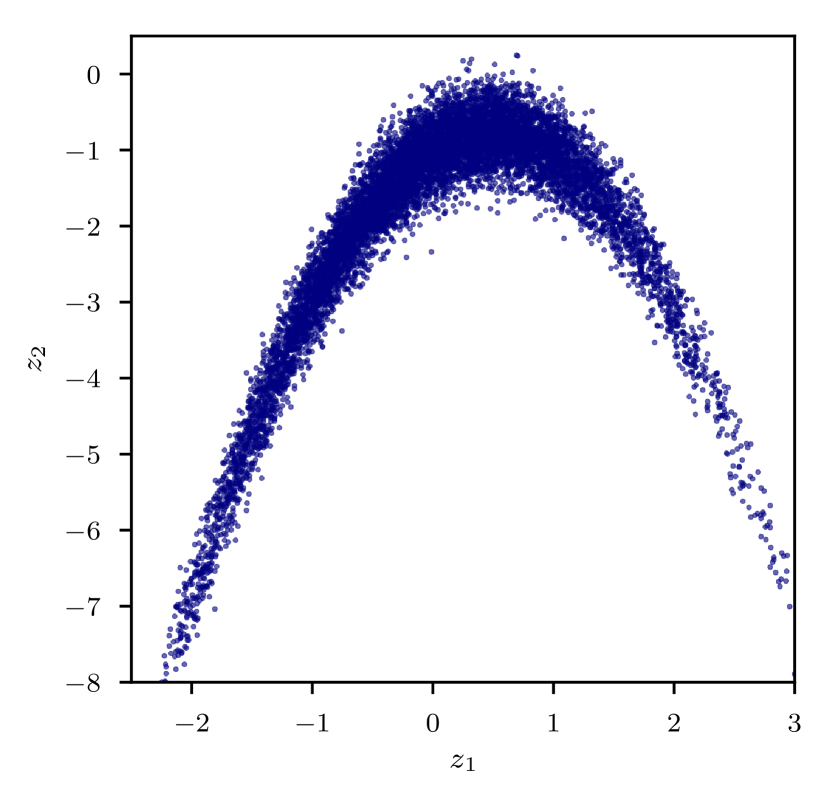
(a) 10k samples from implicit prior $p^{*}({\boldsymbol{\mathbf{z}}})$.

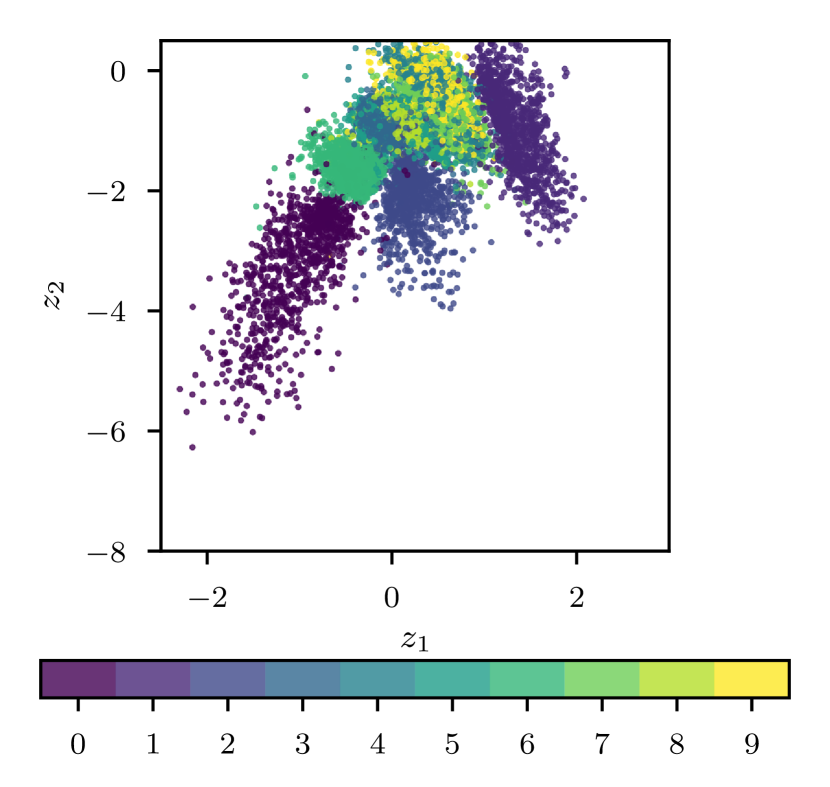
(b) Mean of $q_{{\boldsymbol{\mathbf{\phi}}}}({\boldsymbol{\mathbf{z}}}\,|\,{\boldsymbol{\mathbf{x}}})$ for every ${\boldsymbol{\mathbf{x}}}$ from held-out test set of size 10k, colored by digit class.

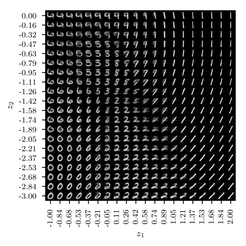
(c) Mean of $p_{{\boldsymbol{\mathbf{\theta}}}}({\boldsymbol{\mathbf{x}}}\,|\,{\boldsymbol{\mathbf{z}}})$ for $20\times 20$ values of ${\boldsymbol{\mathbf{z}}}$ along a uniform grid.

Figure 1: Visualization of 2D latent space and the corresponding observed space manifold.

To empirically assess the performance of our approach, we consider the problem of reducing the dimensionality of the mnist dataset to a 2D latent space, wherein the prior distribution on the latent representations is specified by its samples (shown in fig. 1(a)). This “banana-shaped distribution” is a commonly used testbed for adaptive mcmc methods (Titsias, 2017; Haario et al., 1999). Its samples can be generated by drawing from a bivariate Gaussian with unit variances and correlation $\rho=0.95$, and transforming them through mapping $H(z_{1},z_{2})\coloneqq[z_{1},z_{2}-z_{1}^{2}-1]^{T}$. While the density of this distribution can be computed, it is withheld from our algorithm and used only in the variational autoencoder (vae) baseline, which does not permit implicit distributions. Figure 1(b) shows, for every observation ${\boldsymbol{\mathbf{x}}}$ from a held-out test set, the mean ${\boldsymbol{\mathbf{m}}}_{{\boldsymbol{\mathbf{\phi}}}}({\boldsymbol{\mathbf{x}}})$ of the posterior $q_{{\boldsymbol{\mathbf{\phi}}}}({\boldsymbol{\mathbf{z}}}\,|\,{\boldsymbol{\mathbf{x}}})$ over its underlying latent representation ${\boldsymbol{\mathbf{z}}}$.

Table 1: Mean-squared errors of reconstructions.

Method	mse ${\boldsymbol{\mathbf{z}}}$	mse ${\boldsymbol{\mathbf{x}}}$
sjmvi (ours)	0.17	0.04
vae (Kingma & Welling, 2014)	0.88	0.04
avb (Mescheder et al., 2017)	0.29	0.04

Observe that instances of the various digit classes are disentangled in this latent space, while still closely matching the shape of the prior distribution, despite having only access to its samples. The resulting manifold of reconstructions is depicted in fig. 1(c).

In table 1, we report the mean-squared error (mse) on the reconstructions of observations from the held-out test set and benchmark against vae / avb. Also, for the joint approximation to properly match the support of the exact joint, the latent codes should also be representable by its corresponding observation. Hence, we also report the mse between samples from the prior and their reconstructions. While we find no improvements on reconstruction quality of observations, our method significantly outperforms others in reconstructing latent codes, suggesting our method has greater capacity to faithfully approximate the exact joint.

8 Conclusion

We introduced implicit latent variable models, which offer the greatest extent of flexibility in treatment of prior information, and can be used in to model problems ranging from dimensionality reduction to unpaired image-to-image translation. For their parameter estimation and inference, we developed a variational inference framework that augments traditional vi approaches by minimizing the symmetric kl between the exact joint distribution and an approximate distribution.

Additionally, we provided a theoretical treatment of the link between cyclegans and approximate Bayesian inference. In short, samples from the two domains correspond respectively to those drawn from the data and implicit prior distribution in a ilvm. Parameter learning in cyclegans corresponds to approximate inference in this ilvm under our proposed vi framework. The forward and reverse mappings in cyclegans arise naturally in the generative and recognition models, while the cycle-consistency constraints correspond to their log probabilities, and the adversarial losses are approximations to an $f$-divergence.

By lifting the requirement of prescribed prior distributions in favor of arbitrarily flexible implicit distributions, we can discover different perspectives on existing learning methods and provide more flexible approaches to probabilistic modeling.

Appendix A Graphical Representation

The graphical representation of implicit latent variable models is depicted below in fig. A.2.

(a) Without amortized inference, each local latent variable is governed by its own local variational parameters.

(b) With amortized inference, we condition on observed variables and employ a single set of global variational parameters.

Figure A.2: Graphical representation of the generative model (solid) and the recognition model (dashed).

Appendix B Recovering Common Latent Variable Models

Our model specification is sufficiently general for encapsulating a broad range of familiar latent variable models, even when we make simplifying assumptions on the mapping $\mathcal{F}_{{\boldsymbol{\mathbf{\theta}}}}(\,\cdot\,;{\boldsymbol{\mathbf{z}}})$. In particular, consider the special case where the mapping is an affine transformation of the noise vector ${\boldsymbol{\mathbf{\xi}}}$,

$$\mathcal{F}_{{\boldsymbol{\mathbf{\theta}}}}({\boldsymbol{\mathbf{\xi}}};{\boldsymbol{\mathbf{z}}})\coloneqq{\boldsymbol{\mathbf{\mu}}}_{{\boldsymbol{\mathbf{\theta}}}}({\boldsymbol{\mathbf{z}}})+{\boldsymbol{\mathbf{\Sigma}}}_{{\boldsymbol{\mathbf{\theta}}}}({\boldsymbol{\mathbf{z}}})^{\frac{1}{2}}{\boldsymbol{\mathbf{\xi}}},\quad{\boldsymbol{\mathbf{\xi}}}\sim\mathcal{N}({\boldsymbol{\mathbf{0}}},{\boldsymbol{\mathbf{I}}}),$$

for functions ${\boldsymbol{\mathbf{\mu}}}_{{\boldsymbol{\mathbf{\theta}}}}$ and ${\boldsymbol{\mathbf{\Sigma}}}_{{\boldsymbol{\mathbf{\theta}}}}$ parameterized by ${\boldsymbol{\mathbf{\theta}}}$ that take ${\boldsymbol{\mathbf{z}}}$ as input. To simplify matters further, assume ${\boldsymbol{\mathbf{\Sigma}}}_{{\boldsymbol{\mathbf{\theta}}}}$ is constant w.r.t. to its input, i.e. ${\boldsymbol{\mathbf{\Sigma}}}_{{\boldsymbol{\mathbf{\theta}}}}({\boldsymbol{\mathbf{z}}})={\boldsymbol{\mathbf{\Psi}}}$ for all ${\boldsymbol{\mathbf{z}}}$. The likelihood can then be written explicitly as

$$p_{{\boldsymbol{\mathbf{\theta}}}}({\boldsymbol{\mathbf{x}}}\,|\,{\boldsymbol{\mathbf{z}}})=\mathcal{N}({\boldsymbol{\mathbf{x}}}\,|\,{\boldsymbol{\mathbf{\mu}}}_{{\boldsymbol{\mathbf{\theta}}}}({\boldsymbol{\mathbf{z}}}),{\boldsymbol{\mathbf{\Psi}}}).$$

Factor analysis & probabilistic PCA.  In the case where the mean function ${\boldsymbol{\mathbf{\mu}}}_{{\boldsymbol{\mathbf{\theta}}}}$ is an affine transformation of ${\boldsymbol{\mathbf{z}}}$,

$${\boldsymbol{\mathbf{\mu}}}_{{\boldsymbol{\mathbf{\theta}}}}({\boldsymbol{\mathbf{z}}})\coloneqq{\boldsymbol{\mathbf{W}}}{\boldsymbol{\mathbf{z}}}+{\boldsymbol{\mathbf{b}}},$$

and the covariance matrix is diagonal ${\boldsymbol{\mathbf{\Psi}}}=\textrm{diag}(\psi_{1}^{2},\dotsc,\psi_{D}^{2})$, we recover factor analysis (fa) (Bartholomew et al., 2011). Furthermore, when the covariance matrix is isotropic ${\boldsymbol{\mathbf{\Psi}}}=\psi^{2}{\boldsymbol{\mathbf{I}}}$, we recover ppca (Tipping & Bishop, 1999). In this example, the parameters ${\boldsymbol{\mathbf{\theta}}}$ consist of the factor loading matrix ${\boldsymbol{\mathbf{W}}}$, the bias vector ${\boldsymbol{\mathbf{b}}}$ and the covariance matrix ${\boldsymbol{\mathbf{\Psi}}}$.

Deep and nonlinear latent variable models.  By introducing nonlinearities to the mean function, we are able to recover nonlinear factor analysis (Lappalainen & Honkela, 2000), nonlinear Gaussian sigmoid belief networks (Frey & Hinton, 1999), and other more sophisticated variants of deep latent variable models. When the mapping is defined by a multilayer perceptron (mlp), we can recover simple instances of a vae with a Gaussian probabilistic decoder (Kingma & Welling, 2014; Rezende et al., 2014).

Appendix C Proof of Proposition 1

Proof.

Firstly, note the generative mappings underlying the given Gaussian likelihood and approximate posterior are

$$\begin{split}p_{{\boldsymbol{\mathbf{\theta}}}}({\boldsymbol{\mathbf{x}}}\,|\,{\boldsymbol{\mathbf{z}}})&\coloneqq\mathcal{N}({\boldsymbol{\mathbf{x}}}\,|\,{\boldsymbol{\mathbf{\mu}}}_{{\boldsymbol{\mathbf{\theta}}}}({\boldsymbol{\mathbf{z}}}),\tau^{2}{\boldsymbol{\mathbf{I}}}),\\ \Leftrightarrow\mathcal{F}_{{\boldsymbol{\mathbf{\theta}}}}({\boldsymbol{\mathbf{\xi}}};{\boldsymbol{\mathbf{z}}})&\coloneqq{\boldsymbol{\mathbf{\mu}}}_{{\boldsymbol{\mathbf{\theta}}}}({\boldsymbol{\mathbf{z}}})+\tau{\boldsymbol{\mathbf{\xi}}},\quad{\boldsymbol{\mathbf{\xi}}}\sim\mathcal{N}({\boldsymbol{\mathbf{0}}},{\boldsymbol{\mathbf{I}}}),\end{split}$$

and,

$$\begin{split}q_{{\boldsymbol{\mathbf{\phi}}}}({\boldsymbol{\mathbf{z}}}\,|\,{\boldsymbol{\mathbf{x}}})&\coloneqq\mathcal{N}({\boldsymbol{\mathbf{z}}}\,|\,{\boldsymbol{\mathbf{m}}}_{{\boldsymbol{\mathbf{\phi}}}}({\boldsymbol{\mathbf{x}}}),t^{2}{\boldsymbol{\mathbf{I}}}),\\ \Leftrightarrow\mathcal{G}_{{\boldsymbol{\mathbf{\phi}}}}({\boldsymbol{\mathbf{\epsilon}}};{\boldsymbol{\mathbf{x}}})&\coloneqq{\boldsymbol{\mathbf{m}}}_{{\boldsymbol{\mathbf{\phi}}}}({\boldsymbol{\mathbf{x}}})+t{\boldsymbol{\mathbf{\epsilon}}},\quad{\boldsymbol{\mathbf{\epsilon}}}\sim\mathcal{N}({\boldsymbol{\mathbf{0}}},{\boldsymbol{\mathbf{I}}}),\end{split}$$

respectively. Thus, expanding out $\mathcal{L}_{\textsc{nell}}({\boldsymbol{\mathbf{\theta}}},{\boldsymbol{\mathbf{\phi}}})$, we have

$$\mathcal{L}_{\textsc{nell}}({\boldsymbol{\mathbf{\theta}}},{\boldsymbol{\mathbf{\phi}}}) =\mathbb{E}_{q^{*}({\boldsymbol{\mathbf{x}}})q_{{\boldsymbol{\mathbf{\phi}}}}({\boldsymbol{\mathbf{z}}}\,|\,{\boldsymbol{\mathbf{x}}})}[-\log p_{{\boldsymbol{\mathbf{\theta}}}}({\boldsymbol{\mathbf{x}}}\,|\,{\boldsymbol{\mathbf{z}}})]$$

$$=\mathbb{E}_{q^{*}({\boldsymbol{\mathbf{x}}})p({\boldsymbol{\mathbf{\epsilon}}})}[-\log p_{{\boldsymbol{\mathbf{\theta}}}}({\boldsymbol{\mathbf{x}}}\,|\,\mathcal{G}_{{\boldsymbol{\mathbf{\phi}}}}({\boldsymbol{\mathbf{\epsilon}}};{\boldsymbol{\mathbf{x}}}))]$$

$$\begin{split}&=\frac{1}{2\tau^{2}}\mathbb{E}_{q^{*}({\boldsymbol{\mathbf{x}}})p({\boldsymbol{\mathbf{\epsilon}}})}[\|{\boldsymbol{\mathbf{x}}}-{\boldsymbol{\mathbf{\mu}}}_{{\boldsymbol{\mathbf{\theta}}}}(\mathcal{G}_{{\boldsymbol{\mathbf{\phi}}}}({\boldsymbol{\mathbf{\epsilon}}};{\boldsymbol{\mathbf{x}}}))\|_{2}^{2}]\\ &\qquad+\frac{D}{2}\log 2\pi\tau^{2}\end{split}$$

$$\begin{split}&=\frac{1}{2\tau^{2}}\mathbb{E}_{q^{*}({\boldsymbol{\mathbf{x}}})p({\boldsymbol{\mathbf{\epsilon}}})}[\|{\boldsymbol{\mathbf{x}}}-{\boldsymbol{\mathbf{\mu}}}_{{\boldsymbol{\mathbf{\theta}}}}({\boldsymbol{\mathbf{m}}}_{{\boldsymbol{\mathbf{\phi}}}}({\boldsymbol{\mathbf{x}}})+t{\boldsymbol{\mathbf{\epsilon}}})\|_{2}^{2}]\\ &\qquad+\frac{D}{2}\log 2\pi\tau^{2}\end{split}$$

$$\begin{split}&\to\frac{1}{2\tau^{2}}\mathbb{E}_{q^{*}({\boldsymbol{\mathbf{x}}})}[\|{\boldsymbol{\mathbf{x}}}-{\boldsymbol{\mathbf{\mu}}}_{{\boldsymbol{\mathbf{\theta}}}}({\boldsymbol{\mathbf{m}}}_{{\boldsymbol{\mathbf{\phi}}}}({\boldsymbol{\mathbf{x}}}))\|_{2}^{2}]\\ &\qquad+\frac{D}{2}\log 2\pi\tau^{2},\qquad\textnormal{as }t\to 0\end{split}$$

$$=\gamma_{1}\ell_{\textsc{const}}^{\textnormal{reverse}}({\boldsymbol{\mathbf{\theta}}},{\boldsymbol{\mathbf{\phi}}})+\delta_{1}$$

$$\propto\ell_{\textsc{const}}^{\textnormal{reverse}}({\boldsymbol{\mathbf{\theta}}},{\boldsymbol{\mathbf{\phi}}})$$

where $\gamma_{1}=\frac{1}{2\tau^{2}}$ and $\delta_{1}=\frac{D}{2}\log\frac{\pi}{\gamma_{1}}$.

A similar analysis can be carried out for $\mathcal{L}_{\textsc{nelp}}({\boldsymbol{\mathbf{\theta}}},{\boldsymbol{\mathbf{\phi}}})$ and $\ell_{\textsc{const}}^{\textnormal{forward}}({\boldsymbol{\mathbf{\theta}}},{\boldsymbol{\mathbf{\phi}}})$. ∎

Appendix D Proof of Lemma 1

Proof.

To instantiate $\mathcal{L}_{\textsc{gan}}^{\textnormal{reverse}}({\boldsymbol{\mathbf{\alpha}}}\,|\,{\boldsymbol{\mathbf{\phi}}})$ of eq. 33, it suffices to show that $-f_{\textsc{gan}}^{*}(f_{\textsc{gan}}^{\prime}(r_{{\boldsymbol{\mathbf{\alpha}}}}({\boldsymbol{\mathbf{z}}};{\boldsymbol{\mathbf{x}}})))=\log\mathcal{D}_{{\boldsymbol{\mathbf{\alpha}}}}({\boldsymbol{\mathbf{z}}};{\boldsymbol{\mathbf{x}}})$ and $f_{\textsc{gan}}^{\prime}(r_{{\boldsymbol{\mathbf{\alpha}}}}({\boldsymbol{\mathbf{z}}};{\boldsymbol{\mathbf{x}}}))=\log(1-\mathcal{D}_{{\boldsymbol{\mathbf{\alpha}}}}({\boldsymbol{\mathbf{z}}};{\boldsymbol{\mathbf{x}}}))$, where $\mathcal{D}_{{\boldsymbol{\mathbf{\alpha}}}}({\boldsymbol{\mathbf{z}}};{\boldsymbol{\mathbf{x}}})\coloneqq 1-\sigma(\log r_{{\boldsymbol{\mathbf{\alpha}}}}({\boldsymbol{\mathbf{z}}};{\boldsymbol{\mathbf{x}}}))$. First we compute the first derivative $f_{\textsc{gan}}^{\prime}$ and the convex dual $f_{\textsc{gan}}^{*}$ of $f_{\textsc{gan}}$, which involve straightforward calculations,

$$f_{\textsc{gan}}^{\prime}(u) =\log\sigma(\log u),$$

$$f_{\textsc{gan}}^{*}(t) =-\log(1-\exp t).$$

Thus, the composition $f_{\textsc{gan}}^{*}\circ f_{\textsc{gan}}^{\prime}:u\mapsto f_{\textsc{gan}}^{*}(f_{\textsc{gan}}^{\prime}(u))$ can be simplified as

$$f_{\textsc{gan}}^{*}(f_{\textsc{gan}}^{\prime}(u)) =-\log(1-\exp f_{\textsc{gan}}^{\prime}(u))$$

$$=-\log(1-\sigma(\log u)).$$

Applying $f_{\textsc{gan}}^{\prime}$ and $f_{\textsc{gan}}^{*}\circ f_{\textsc{gan}}^{\prime}$ to $r_{{\boldsymbol{\mathbf{\alpha}}}}({\boldsymbol{\mathbf{z}}};{\boldsymbol{\mathbf{x}}})$, we have

$$f_{\textsc{gan}}^{\prime}(r_{{\boldsymbol{\mathbf{\alpha}}}}({\boldsymbol{\mathbf{z}}};{\boldsymbol{\mathbf{x}}})) =\log\sigma(\log r_{{\boldsymbol{\mathbf{\alpha}}}}({\boldsymbol{\mathbf{z}}};{\boldsymbol{\mathbf{x}}}))$$

$$=\log(1-\mathcal{D}_{{\boldsymbol{\mathbf{\alpha}}}}({\boldsymbol{\mathbf{z}}};{\boldsymbol{\mathbf{x}}})),$$

and

$$f_{\textsc{gan}}^{*}(f_{\textsc{gan}}^{\prime}(r_{{\boldsymbol{\mathbf{\alpha}}}}({\boldsymbol{\mathbf{z}}};{\boldsymbol{\mathbf{x}}}))) =-\log(1-\sigma(\log r_{{\boldsymbol{\mathbf{\alpha}}}}({\boldsymbol{\mathbf{z}}};{\boldsymbol{\mathbf{x}}})))$$

$$=-\log\mathcal{D}_{{\boldsymbol{\mathbf{\alpha}}}}({\boldsymbol{\mathbf{z}}};{\boldsymbol{\mathbf{x}}}),$$

respectively, as required. ∎

Appendix E Proof of Lemma 2

Proof.

Through reparameterization of $q_{{\boldsymbol{\mathbf{\phi}}}}({\boldsymbol{\mathbf{z}}}\,|\,{\boldsymbol{\mathbf{x}}})$, we have

$$\begin{split}\mathcal{L}_{\textsc{gan}}^{\textnormal{reverse}}({\boldsymbol{\mathbf{\alpha}}}\,|\,{\boldsymbol{\mathbf{\phi}}})&=\mathbb{E}_{q^{*}({\boldsymbol{\mathbf{x}}})p^{*}({\boldsymbol{\mathbf{z}}})}[\log\mathcal{D}_{{\boldsymbol{\mathbf{\alpha}}}}({\boldsymbol{\mathbf{z}}};{\boldsymbol{\mathbf{x}}})]\\ &+\mathbb{E}_{q^{*}({\boldsymbol{\mathbf{x}}})p({\boldsymbol{\mathbf{\epsilon}}})}[\log(1-\mathcal{D}_{{\boldsymbol{\mathbf{\alpha}}}}(\mathcal{G}_{{\boldsymbol{\mathbf{\phi}}}}({\boldsymbol{\mathbf{\epsilon}}};{\boldsymbol{\mathbf{x}}});{\boldsymbol{\mathbf{x}}}))].\end{split}$$

By specifying a discriminator $\mathcal{D}_{{\boldsymbol{\mathbf{\alpha}}}}({\boldsymbol{\mathbf{z}}};{\boldsymbol{\mathbf{x}}})={\boldsymbol{\mathbf{D}}}_{{\boldsymbol{\mathbf{\alpha}}}}({\boldsymbol{\mathbf{z}}})$ which ignores auxiliary input ${\boldsymbol{\mathbf{x}}}$, and mapping $\mathcal{G}_{{\boldsymbol{\mathbf{\phi}}}}({\boldsymbol{\mathbf{\epsilon}}};{\boldsymbol{\mathbf{x}}})={\boldsymbol{\mathbf{m}}}_{{\boldsymbol{\mathbf{\phi}}}}({\boldsymbol{\mathbf{x}}})$ which ignores noise input ${\boldsymbol{\mathbf{\epsilon}}}$, this reduces to

$$\begin{split}\mathcal{L}_{\textsc{gan}}^{\textnormal{reverse}}({\boldsymbol{\mathbf{\alpha}}}\,|\,{\boldsymbol{\mathbf{\phi}}})&=\mathbb{E}_{p^{*}({\boldsymbol{\mathbf{z}}})}[\log{\boldsymbol{\mathbf{D}}}_{{\boldsymbol{\mathbf{\alpha}}}}({\boldsymbol{\mathbf{z}}})]\\ &+\mathbb{E}_{q^{*}({\boldsymbol{\mathbf{x}}})}[\log(1-{\boldsymbol{\mathbf{D}}}_{{\boldsymbol{\mathbf{\alpha}}}}({\boldsymbol{\mathbf{m}}}_{{\boldsymbol{\mathbf{\phi}}}}({\boldsymbol{\mathbf{x}}})))]\end{split}$$

$$=\ell_{\textsc{gan}}^{\textnormal{reverse}}({\boldsymbol{\mathbf{\alpha}}}\,|\,{\boldsymbol{\mathbf{\phi}}}),$$

as required. ∎

Appendix F Proof of Proposition 3

Proof.

Expanding out $\mathcal{L}_{\textsc{gan}_{\textsc{C}}}^{\textnormal{reverse}}({\boldsymbol{\mathbf{\phi}}}\,|\,{\boldsymbol{\mathbf{\alpha}}})$, we have

$$\mathcal{L}_{\textsc{gan}_{\textsc{C}}}^{\textnormal{reverse}}({\boldsymbol{\mathbf{\phi}}}\,|\,{\boldsymbol{\mathbf{\alpha}}}) =\mathbb{E}_{q^{*}({\boldsymbol{\mathbf{x}}})q_{{\boldsymbol{\mathbf{\phi}}}}({\boldsymbol{\mathbf{z}}}\,|\,{\boldsymbol{\mathbf{x}}})}\left[-\log\frac{\mathcal{D}_{{\boldsymbol{\mathbf{\alpha}}}}({\boldsymbol{\mathbf{z}}};{\boldsymbol{\mathbf{x}}})}{1-\mathcal{D}_{{\boldsymbol{\mathbf{\alpha}}}}({\boldsymbol{\mathbf{z}}};{\boldsymbol{\mathbf{x}}})}\right]$$

$$=\mathbb{E}_{q^{*}({\boldsymbol{\mathbf{x}}})q_{{\boldsymbol{\mathbf{\phi}}}}({\boldsymbol{\mathbf{z}}}\,|\,{\boldsymbol{\mathbf{x}}})}\left[\log\frac{\sigma(\log r_{{\boldsymbol{\mathbf{\alpha}}}}({\boldsymbol{\mathbf{z}}};{\boldsymbol{\mathbf{x}}}))}{1-\sigma(\log r_{{\boldsymbol{\mathbf{\alpha}}}}({\boldsymbol{\mathbf{z}}};{\boldsymbol{\mathbf{x}}}))}\right]$$

$$=\mathbb{E}_{q^{*}({\boldsymbol{\mathbf{x}}})q_{{\boldsymbol{\mathbf{\phi}}}}({\boldsymbol{\mathbf{z}}}\,|\,{\boldsymbol{\mathbf{x}}})}[\log r_{{\boldsymbol{\mathbf{\alpha}}}}({\boldsymbol{\mathbf{z}}};{\boldsymbol{\mathbf{x}}})]$$

$$\coloneqq\mathcal{L}_{\textsc{kl}}^{\textnormal{latent}}({\boldsymbol{\mathbf{\phi}}}\,|\,{\boldsymbol{\mathbf{\alpha}}}).$$

Hence, $\mathcal{L}_{\textsc{gan}_{\textsc{C}}}^{\textnormal{reverse}}({\boldsymbol{\mathbf{\phi}}}\,|\,{\boldsymbol{\mathbf{\alpha}}})=\mathcal{L}_{\textsc{kl}}^{\textnormal{latent}}({\boldsymbol{\mathbf{\phi}}}\,|\,{\boldsymbol{\mathbf{\alpha}}})$ as required. ∎

Appendix G Relation to KL Importance Estimation Procedure (KLIEP)

We now discuss the connections to kliep (Sugiyama et al., 2008). Consider the same problem setting as in § 3.3 where we wish to use a parameterized function $r_{{\boldsymbol{\mathbf{\alpha}}}}$ to estimate the exact density ratio,

$$r_{{\boldsymbol{\mathbf{\alpha}}}}({\boldsymbol{\mathbf{z}}};{\boldsymbol{\mathbf{x}}})\simeq r^{*}({\boldsymbol{\mathbf{z}}};{\boldsymbol{\mathbf{x}}})\coloneqq\frac{q_{{\boldsymbol{\mathbf{\phi}}}}({\boldsymbol{\mathbf{z}}}\,|\,{\boldsymbol{\mathbf{x}}})}{p^{*}({\boldsymbol{\mathbf{z}}})}.$$

We can view $r_{{\boldsymbol{\mathbf{\alpha}}}}({\boldsymbol{\mathbf{z}}};{\boldsymbol{\mathbf{x}}})$ as the correction factor required for $p^{*}({\boldsymbol{\mathbf{z}}})$ to match $q_{{\boldsymbol{\mathbf{\phi}}}}({\boldsymbol{\mathbf{z}}}\,|\,{\boldsymbol{\mathbf{x}}})$. This gives rise to an estimator of $q_{{\boldsymbol{\mathbf{\phi}}}}({\boldsymbol{\mathbf{z}}}\,|\,{\boldsymbol{\mathbf{x}}})$,

$$q_{{\boldsymbol{\mathbf{\alpha}}}}({\boldsymbol{\mathbf{z}}}\,|\,{\boldsymbol{\mathbf{x}}})\coloneqq r_{{\boldsymbol{\mathbf{\alpha}}}}({\boldsymbol{\mathbf{z}}};{\boldsymbol{\mathbf{x}}})p^{*}({\boldsymbol{\mathbf{z}}})\simeq q_{{\boldsymbol{\mathbf{\phi}}}}({\boldsymbol{\mathbf{z}}}\,|\,{\boldsymbol{\mathbf{x}}}).$$

Although in our specific problem setting, the density $q_{{\boldsymbol{\mathbf{\phi}}}}({\boldsymbol{\mathbf{z}}}\,|\,{\boldsymbol{\mathbf{x}}})$ is tractable, we nonetheless fit an auxiliary model $q_{{\boldsymbol{\mathbf{\alpha}}}}({\boldsymbol{\mathbf{z}}}\,|\,{\boldsymbol{\mathbf{x}}})$ to it as a means of fitting the underlying density ratio estimator $r_{{\boldsymbol{\mathbf{\alpha}}}}({\boldsymbol{\mathbf{z}}};{\boldsymbol{\mathbf{x}}})$.

In particular, consider minimizing the kl divergence between $q_{{\boldsymbol{\mathbf{\phi}}}}({\boldsymbol{\mathbf{z}}}\,|\,{\boldsymbol{\mathbf{x}}})$ and $q_{{\boldsymbol{\mathbf{\alpha}}}}({\boldsymbol{\mathbf{z}}}\,|\,{\boldsymbol{\mathbf{x}}})$ with respect to ${\boldsymbol{\mathbf{\alpha}}}$,

$$\begin{split}\mathbb{E}_{q^{*}({\boldsymbol{\mathbf{x}}})}&\textsc{kl}\left[q_{{\boldsymbol{\mathbf{\phi}}}}({\boldsymbol{\mathbf{z}}}\,|\,{\boldsymbol{\mathbf{x}}})\;\|\;q_{{\boldsymbol{\mathbf{\alpha}}}}({\boldsymbol{\mathbf{z}}}\,|\,{\boldsymbol{\mathbf{x}}})\right]\\ &\coloneqq\mathbb{E}_{q^{*}({\boldsymbol{\mathbf{x}}})}\mathbb{E}_{q_{{\boldsymbol{\mathbf{\phi}}}}({\boldsymbol{\mathbf{z}}}\,|\,{\boldsymbol{\mathbf{x}}})}\left[\log\frac{q_{{\boldsymbol{\mathbf{\phi}}}}({\boldsymbol{\mathbf{z}}}\,|\,{\boldsymbol{\mathbf{x}}})}{q_{{\boldsymbol{\mathbf{\alpha}}}}({\boldsymbol{\mathbf{z}}}\,|\,{\boldsymbol{\mathbf{x}}})}\right],\end{split}$$

$$\begin{split}&=\mathbb{E}_{q^{*}({\boldsymbol{\mathbf{x}}})}\mathbb{E}_{q_{{\boldsymbol{\mathbf{\phi}}}}({\boldsymbol{\mathbf{z}}}\,|\,{\boldsymbol{\mathbf{x}}})}\left[\log\frac{q_{{\boldsymbol{\mathbf{\phi}}}}({\boldsymbol{\mathbf{z}}}\,|\,{\boldsymbol{\mathbf{x}}})}{p^{*}({\boldsymbol{\mathbf{z}}})r_{{\boldsymbol{\mathbf{\alpha}}}}({\boldsymbol{\mathbf{z}}};{\boldsymbol{\mathbf{x}}})}\right],\end{split}$$

$$\begin{split}&=-\mathbb{E}_{q^{*}({\boldsymbol{\mathbf{x}}})}\mathbb{E}_{q_{{\boldsymbol{\mathbf{\phi}}}}({\boldsymbol{\mathbf{z}}}\,|\,{\boldsymbol{\mathbf{x}}})}[\log r_{{\boldsymbol{\mathbf{\alpha}}}}({\boldsymbol{\mathbf{z}}};{\boldsymbol{\mathbf{x}}})]+\textrm{const}.\end{split}$$

Hence, this is equivalent to maximizing

$$\mathbb{E}_{q^{*}({\boldsymbol{\mathbf{x}}})}\mathbb{E}_{q_{{\boldsymbol{\mathbf{\phi}}}}({\boldsymbol{\mathbf{z}}}\,|\,{\boldsymbol{\mathbf{x}}})}[\log r_{{\boldsymbol{\mathbf{\alpha}}}}({\boldsymbol{\mathbf{z}}};{\boldsymbol{\mathbf{x}}})].$$

Now, for the conditional $q_{{\boldsymbol{\mathbf{\alpha}}}}({\boldsymbol{\mathbf{z}}}\,|\,{\boldsymbol{\mathbf{x}}})$ to be a probability density function, its integral must sum to one,

$$\int q_{{\boldsymbol{\mathbf{\alpha}}}}({\boldsymbol{\mathbf{z}}}\,|\,{\boldsymbol{\mathbf{x}}})q^{*}({\boldsymbol{\mathbf{x}}})d{\boldsymbol{\mathbf{x}}}d{\boldsymbol{\mathbf{z}}}=1.$$

Rewriting this integral, we have the constraint

$$\int q_{{\boldsymbol{\mathbf{\alpha}}}}({\boldsymbol{\mathbf{z}}}\,|\,{\boldsymbol{\mathbf{x}}})q^{*}({\boldsymbol{\mathbf{x}}})d{\boldsymbol{\mathbf{x}}}d{\boldsymbol{\mathbf{z}}} =\int r_{{\boldsymbol{\mathbf{\alpha}}}}({\boldsymbol{\mathbf{z}}};{\boldsymbol{\mathbf{x}}})p^{*}({\boldsymbol{\mathbf{z}}})q^{*}({\boldsymbol{\mathbf{x}}})d{\boldsymbol{\mathbf{x}}}d{\boldsymbol{\mathbf{z}}}$$

$$=\mathbb{E}_{q^{*}({\boldsymbol{\mathbf{x}}})p^{*}({\boldsymbol{\mathbf{z}}})}[r_{{\boldsymbol{\mathbf{\alpha}}}}({\boldsymbol{\mathbf{z}}};{\boldsymbol{\mathbf{x}}})]=1.$$

Combined, we have the following constrained optimization problem,

$$\max_{{\boldsymbol{\mathbf{\alpha}}}}\qquad \mathbb{E}_{q^{*}({\boldsymbol{\mathbf{x}}})}\mathbb{E}_{q_{{\boldsymbol{\mathbf{\phi}}}}({\boldsymbol{\mathbf{z}}}\,|\,{\boldsymbol{\mathbf{x}}})}[\log r_{{\boldsymbol{\mathbf{\alpha}}}}({\boldsymbol{\mathbf{z}}};{\boldsymbol{\mathbf{x}}})]$$

subject to $$\mathbb{E}_{q^{*}({\boldsymbol{\mathbf{x}}})p^{*}({\boldsymbol{\mathbf{z}}})}[r_{{\boldsymbol{\mathbf{\alpha}}}}({\boldsymbol{\mathbf{z}}};{\boldsymbol{\mathbf{x}}})-1]=0.$$

Through the method of Lagrange multipliers, this can be cast as an unconstrained optimization problem with objective,

$$\begin{split}\mathcal{L}_{\textsc{kliep}}^{\textnormal{latent}}({\boldsymbol{\mathbf{\alpha}}}\,|\,{\boldsymbol{\mathbf{\phi}}})&\coloneqq\mathbb{E}_{q^{*}({\boldsymbol{\mathbf{x}}})}\mathbb{E}_{q_{{\boldsymbol{\mathbf{\phi}}}}({\boldsymbol{\mathbf{z}}}\,|\,{\boldsymbol{\mathbf{x}}})}[\log r_{{\boldsymbol{\mathbf{\alpha}}}}({\boldsymbol{\mathbf{z}}};{\boldsymbol{\mathbf{x}}})]\\ &\qquad-\lambda\mathbb{E}_{q^{*}({\boldsymbol{\mathbf{x}}})p^{*}({\boldsymbol{\mathbf{z}}})}[r_{{\boldsymbol{\mathbf{\alpha}}}}({\boldsymbol{\mathbf{z}}};{\boldsymbol{\mathbf{x}}})-1],\end{split}$$

where $\lambda$ is the Lagrange multiplier. For $\lambda=1$, $\mathcal{L}_{\textsc{kliep}}^{\textnormal{latent}}({\boldsymbol{\mathbf{\alpha}}}\,|\,{\boldsymbol{\mathbf{\phi}}})$ trivially reduces to $\mathcal{L}_{\textsc{kl}}^{\textnormal{latent}}({\boldsymbol{\mathbf{\alpha}}}\,|\,{\boldsymbol{\mathbf{\phi}}})$.

Appendix H Summary of Definitions

In this section, we summarize the definitions of the losses defined in the proposed vi framework of §§ 3 and 4, and underscore the relationships to their respective counterparts in the cyclegan framework of § 5.

Table 2: Relevant latent and observed space $f$-divergences instantiated for particular settings of $f$.

		Reverse kl	gan
	$f(u)$	$\displaystyle u\log u$	$\displaystyle u\log u-(u+1)\log(u+1)$
Latent	$\displaystyle\mathbb{E}_{q^{*}({\boldsymbol{\mathbf{x}}})}\mathcal{D}_{f}\left[p^{*}({\boldsymbol{\mathbf{z}}})\;\|\;q_{{\boldsymbol{\mathbf{\phi}}}}({\boldsymbol{\mathbf{z}}}\,|\,{\boldsymbol{\mathbf{x}}})\right]$	$\displaystyle\mathbb{E}_{q^{*}({\boldsymbol{\mathbf{x}}})}\textsc{kl}\left[q_{{\boldsymbol{\mathbf{\phi}}}}({\boldsymbol{\mathbf{z}}}\,|\,{\boldsymbol{\mathbf{x}}})\;\|\;p^{*}({\boldsymbol{\mathbf{z}}})\right]$	$\displaystyle 2\cdot\mathbb{E}_{q^{*}({\boldsymbol{\mathbf{x}}})}\textsc{js}\left[p^{*}({\boldsymbol{\mathbf{z}}})\;\|\;q_{{\boldsymbol{\mathbf{\phi}}}}({\boldsymbol{\mathbf{z}}}\,|\,{\boldsymbol{\mathbf{x}}})\right]-\log 4$
Observed	$\displaystyle\mathbb{E}_{p^{*}({\boldsymbol{\mathbf{z}}})}\mathcal{D}_{f}\left[q^{*}({\boldsymbol{\mathbf{x}}})\;\|\;p_{{\boldsymbol{\mathbf{\theta}}}}({\boldsymbol{\mathbf{x}}}\,|\,{\boldsymbol{\mathbf{z}}})\right]$	$\displaystyle\mathbb{E}_{p^{*}({\boldsymbol{\mathbf{z}}})}\textsc{kl}\left[p_{{\boldsymbol{\mathbf{\theta}}}}({\boldsymbol{\mathbf{x}}}\,|\,{\boldsymbol{\mathbf{z}}})\;\|\;q^{*}({\boldsymbol{\mathbf{x}}})\right]$	$\displaystyle 2\cdot\mathbb{E}_{p^{*}({\boldsymbol{\mathbf{z}}})}\textsc{js}\left[q^{*}({\boldsymbol{\mathbf{x}}})\;\|\;p_{{\boldsymbol{\mathbf{\theta}}}}({\boldsymbol{\mathbf{x}}}\,|\,{\boldsymbol{\mathbf{z}}})\right]-\log 4$

Table 2 summarizes the settings of convex function $f:\mathbb{R}_{+}\to\mathbb{R}$ that recover the reverse kl divergence terms within the elbo and aplbo, and the Jensen-Shannon (js) divergence (up to constants) that gans are known to minimize.

Table 3: Calculations for convex functions.

	Reverse kl	gan
$\displaystyle f(u)$	$\displaystyle u\log u$	$\displaystyle u\log u-(u+1)\log(u+1)$
$\displaystyle f^{\star}(t)$	$\displaystyle\exp(t-1)$	$\displaystyle-\log(1-\exp t)$
$\displaystyle f^{\prime}(u)$	$\displaystyle 1+\log u$	$\displaystyle\log\sigma(\log u)$
$\displaystyle f^{\star}(f^{\prime}(u))$	$\displaystyle u$	$\displaystyle-\log(1-\sigma(\log u))$

Table 3 gives the calculations of the terms necessary to explicitly write down instances of the generalized variational lower bound for particular convex functions $f$—namely the convex dual $f^{\star}$, the first derivative $f^{\prime}$ and the composition $f^{\star}\circ f^{\prime}$.

Table 4 gives instances of the variational lower bound that approximate the latent and observed space kl divergences within the elbo and aplbo, respectively. Additionally, it gives generalized stochastic formulations of the gan objectives in the cyclegan framework, while table 5 lists their deterministic counterpart.

Lastly, table 6 gives forward and reverse cycle-consistency constraints in the cyclegan framework, and the specific class of Gaussian likelihoods and posteriors that instantiates these constraints (in the limit).

Table 4: Instances of variational lower bounds on the relevant latent and observed space $f$-divergences.

		Reverse kl	gan
	$f(u)$	$\displaystyle u\log u$	$\displaystyle u\log u-(u+1)\log(u+1)$
Latent	$\begin{aligned} \mathcal{L}_{f}^{\textnormal{latent}}({\boldsymbol{\mathbf{\alpha}}}\,|\,{\boldsymbol{\mathbf{\phi}}})&\coloneqq\mathbb{E}_{q^{*}({\boldsymbol{\mathbf{x}}})q_{{\boldsymbol{\mathbf{\phi}}}}({\boldsymbol{\mathbf{z}}}\,|\,{\boldsymbol{\mathbf{x}}})}[f^{\prime}(r_{{\boldsymbol{\mathbf{\alpha}}}}({\boldsymbol{\mathbf{z}}};{\boldsymbol{\mathbf{x}}}))]\\ &\quad-\mathbb{E}_{q^{*}({\boldsymbol{\mathbf{x}}})p^{*}({\boldsymbol{\mathbf{z}}})}[f^{\star}(f^{\prime}(r_{{\boldsymbol{\mathbf{\alpha}}}}({\boldsymbol{\mathbf{z}}};{\boldsymbol{\mathbf{x}}})))]\end{aligned}$	$\begin{aligned} \mathcal{L}_{\textsc{kl}}^{\textnormal{latent}}({\boldsymbol{\mathbf{\alpha}}}\,|\,{\boldsymbol{\mathbf{\phi}}})&\coloneqq\mathbb{E}_{q^{*}({\boldsymbol{\mathbf{x}}})q_{{\boldsymbol{\mathbf{\phi}}}}({\boldsymbol{\mathbf{z}}}\,|\,{\boldsymbol{\mathbf{x}}})}[\log r_{{\boldsymbol{\mathbf{\alpha}}}}({\boldsymbol{\mathbf{z}}};{\boldsymbol{\mathbf{x}}})]\\ &\quad-\mathbb{E}_{q^{*}({\boldsymbol{\mathbf{x}}})p^{*}({\boldsymbol{\mathbf{z}}})}[r_{{\boldsymbol{\mathbf{\alpha}}}}({\boldsymbol{\mathbf{z}}};{\boldsymbol{\mathbf{x}}})-1]\end{aligned}$	$\begin{aligned} \mathcal{L}_{\textsc{gan}}^{\textnormal{reverse}}({\boldsymbol{\mathbf{\alpha}}}\,|\,{\boldsymbol{\mathbf{\phi}}})&\coloneqq\mathbb{E}_{q^{*}({\boldsymbol{\mathbf{x}}})q_{{\boldsymbol{\mathbf{\phi}}}}({\boldsymbol{\mathbf{z}}}\,|\,{\boldsymbol{\mathbf{x}}})}[\log\sigma(\log r_{{\boldsymbol{\mathbf{\alpha}}}}({\boldsymbol{\mathbf{z}}};{\boldsymbol{\mathbf{x}}}))]\\ &+\mathbb{E}_{q^{*}({\boldsymbol{\mathbf{x}}})p^{*}({\boldsymbol{\mathbf{z}}})}[\log(1-\sigma(\log r_{{\boldsymbol{\mathbf{\alpha}}}}({\boldsymbol{\mathbf{z}}};{\boldsymbol{\mathbf{x}}})))]\end{aligned}$
Observed	$\begin{aligned} \mathcal{L}_{f}^{\textnormal{observed}}({\boldsymbol{\mathbf{\beta}}}\,|\,{\boldsymbol{\mathbf{\theta}}})&\coloneqq\mathbb{E}_{p^{*}({\boldsymbol{\mathbf{z}}})p_{{\boldsymbol{\mathbf{\theta}}}}({\boldsymbol{\mathbf{x}}}\,|\,{\boldsymbol{\mathbf{z}}})}[f^{\prime}(r_{{\boldsymbol{\mathbf{\beta}}}}({\boldsymbol{\mathbf{x}}};{\boldsymbol{\mathbf{z}}}))]\\ &\quad-\mathbb{E}_{p^{*}({\boldsymbol{\mathbf{z}}})q^{*}({\boldsymbol{\mathbf{x}}})}[f^{\star}(f^{\prime}(r_{{\boldsymbol{\mathbf{\beta}}}}({\boldsymbol{\mathbf{x}}};{\boldsymbol{\mathbf{z}}})))]\end{aligned}$	$\begin{aligned} \mathcal{L}_{\textsc{kl}}^{\textnormal{observed}}({\boldsymbol{\mathbf{\beta}}}\,|\,{\boldsymbol{\mathbf{\theta}}})&\coloneqq\mathbb{E}_{p^{*}({\boldsymbol{\mathbf{z}}})p_{{\boldsymbol{\mathbf{\theta}}}}({\boldsymbol{\mathbf{x}}}\,|\,{\boldsymbol{\mathbf{z}}})}[\log r_{{\boldsymbol{\mathbf{\beta}}}}({\boldsymbol{\mathbf{x}}};{\boldsymbol{\mathbf{z}}})]\\ &\quad-\mathbb{E}_{p^{*}({\boldsymbol{\mathbf{z}}})q^{*}({\boldsymbol{\mathbf{x}}})}[r_{{\boldsymbol{\mathbf{\beta}}}}({\boldsymbol{\mathbf{x}}};{\boldsymbol{\mathbf{z}}})-1]\end{aligned}$	$\begin{aligned} \mathcal{L}_{\textsc{gan}}^{\textnormal{forward}}({\boldsymbol{\mathbf{\beta}}}\,|\,{\boldsymbol{\mathbf{\theta}}})&\coloneqq\mathbb{E}_{p^{*}({\boldsymbol{\mathbf{z}}})p_{{\boldsymbol{\mathbf{\theta}}}}({\boldsymbol{\mathbf{x}}}\,|\,{\boldsymbol{\mathbf{z}}})}[\log\sigma(\log r_{{\boldsymbol{\mathbf{\beta}}}}({\boldsymbol{\mathbf{x}}};{\boldsymbol{\mathbf{z}}}))]\\ &+\mathbb{E}_{p^{*}({\boldsymbol{\mathbf{z}}})q^{*}({\boldsymbol{\mathbf{x}}})}[\log(1-\sigma(\log r_{{\boldsymbol{\mathbf{\beta}}}}({\boldsymbol{\mathbf{x}}};{\boldsymbol{\mathbf{z}}})))]\end{aligned}$

Table 5: General stochastic gan objectives and their deterministic counterparts.

	Stochastic	Deterministic
reverse	$\begin{aligned} \mathcal{L}_{\textsc{gan}}^{\textnormal{reverse}}({\boldsymbol{\mathbf{\alpha}}}\,|\,{\boldsymbol{\mathbf{\phi}}})&\coloneqq\mathbb{E}_{q^{*}({\boldsymbol{\mathbf{x}}})p^{*}({\boldsymbol{\mathbf{z}}})}[\log\mathcal{D}_{{\boldsymbol{\mathbf{\alpha}}}}({\boldsymbol{\mathbf{z}}};{\boldsymbol{\mathbf{x}}})]\\ &+\mathbb{E}_{q^{*}({\boldsymbol{\mathbf{x}}})p({\boldsymbol{\mathbf{\epsilon}}})}[\log(1-\mathcal{D}_{{\boldsymbol{\mathbf{\alpha}}}}(\mathcal{G}_{{\boldsymbol{\mathbf{\phi}}}}({\boldsymbol{\mathbf{\epsilon}}};{\boldsymbol{\mathbf{x}}});{\boldsymbol{\mathbf{x}}}))]\end{aligned}$	$\begin{aligned} \ell_{\textsc{gan}}^{\textnormal{reverse}}({\boldsymbol{\mathbf{\alpha}}}\,|\,{\boldsymbol{\mathbf{\phi}}})&\coloneqq\mathbb{E}_{p^{*}({\boldsymbol{\mathbf{z}}})}[\log{\boldsymbol{\mathbf{D}}}_{{\boldsymbol{\mathbf{\alpha}}}}({\boldsymbol{\mathbf{z}}})]\\ &\quad+\mathbb{E}_{q^{*}({\boldsymbol{\mathbf{x}}})}[\log(1-{\boldsymbol{\mathbf{D}}}_{{\boldsymbol{\mathbf{\alpha}}}}({\boldsymbol{\mathbf{m}}}_{{\boldsymbol{\mathbf{\phi}}}}({\boldsymbol{\mathbf{x}}})))]\end{aligned}$
forward	$\begin{aligned} \mathcal{L}_{\textsc{gan}}^{\textnormal{forward}}({\boldsymbol{\mathbf{\beta}}}\,|\,{\boldsymbol{\mathbf{\theta}}})&\coloneqq\mathbb{E}_{p^{*}({\boldsymbol{\mathbf{z}}})q^{*}({\boldsymbol{\mathbf{x}}})}[\log\mathcal{D}_{{\boldsymbol{\mathbf{\beta}}}}({\boldsymbol{\mathbf{x}}};{\boldsymbol{\mathbf{z}}})]\\ &+\mathbb{E}_{p^{*}({\boldsymbol{\mathbf{z}}})p({\boldsymbol{\mathbf{\xi}}})}[\log(1-\mathcal{D}_{{\boldsymbol{\mathbf{\beta}}}}(\mathcal{F}_{{\boldsymbol{\mathbf{\theta}}}}({\boldsymbol{\mathbf{\xi}}};{\boldsymbol{\mathbf{z}}});{\boldsymbol{\mathbf{z}}}))]\end{aligned}$	$\begin{aligned} \ell_{\textsc{gan}}^{\textnormal{forward}}({\boldsymbol{\mathbf{\beta}}}\,|\,{\boldsymbol{\mathbf{\theta}}})&\coloneqq\mathbb{E}_{p^{*}({\boldsymbol{\mathbf{x}}})}[\log{\boldsymbol{\mathbf{D}}}_{{\boldsymbol{\mathbf{\beta}}}}({\boldsymbol{\mathbf{x}}})]\\ &\quad+\mathbb{E}_{p^{*}({\boldsymbol{\mathbf{z}}})}[\log(1-{\boldsymbol{\mathbf{D}}}_{{\boldsymbol{\mathbf{\beta}}}}({\boldsymbol{\mathbf{\mu}}}_{{\boldsymbol{\mathbf{\theta}}}}({\boldsymbol{\mathbf{z}}})))]\end{aligned}$

Table 6: Negative expected log conditionals and the cycle-consistency constraints.

Gaussian		Degenerate
$p_{{\boldsymbol{\mathbf{\theta}}}}({\boldsymbol{\mathbf{x}}}\,|\,{\boldsymbol{\mathbf{z}}})$	$q_{{\boldsymbol{\mathbf{\phi}}}}({\boldsymbol{\mathbf{z}}}\,|\,{\boldsymbol{\mathbf{x}}})$	$p_{{\boldsymbol{\mathbf{\theta}}}}({\boldsymbol{\mathbf{x}}}\,|\,{\boldsymbol{\mathbf{z}}})$	$q_{{\boldsymbol{\mathbf{\phi}}}}({\boldsymbol{\mathbf{z}}}\,|\,{\boldsymbol{\mathbf{x}}})$
$\mathcal{N}({\boldsymbol{\mathbf{x}}}\,|\,{\boldsymbol{\mathbf{\mu}}}_{{\boldsymbol{\mathbf{\theta}}}}({\boldsymbol{\mathbf{z}}}),\tau^{2}{\boldsymbol{\mathbf{I}}})$	$\mathcal{N}({\boldsymbol{\mathbf{z}}}\,|\,{\boldsymbol{\mathbf{m}}}_{{\boldsymbol{\mathbf{\phi}}}}({\boldsymbol{\mathbf{x}}}),t^{2}{\boldsymbol{\mathbf{I}}})$	$\to\delta({\boldsymbol{\mathbf{x}}}-{\boldsymbol{\mathbf{\mu}}}_{{\boldsymbol{\mathbf{\theta}}}}({\boldsymbol{\mathbf{z}}}))$	$\to\delta({\boldsymbol{\mathbf{z}}}-{\boldsymbol{\mathbf{m}}}_{{\boldsymbol{\mathbf{\phi}}}}({\boldsymbol{\mathbf{x}}}))$
$\begin{aligned} \mathcal{L}_{\textsc{nell}}({\boldsymbol{\mathbf{\theta}}},{\boldsymbol{\mathbf{\phi}}})\coloneqq\frac{1}{2\tau^{2}}\mathbb{E}_{q^{*}({\boldsymbol{\mathbf{x}}})p({\boldsymbol{\mathbf{\epsilon}}})}[\|{\boldsymbol{\mathbf{x}}}-{\boldsymbol{\mathbf{\mu}}}_{{\boldsymbol{\mathbf{\theta}}}}({\boldsymbol{\mathbf{m}}}_{{\boldsymbol{\mathbf{\phi}}}}({\boldsymbol{\mathbf{x}}})+t{\boldsymbol{\mathbf{\epsilon}}})\|_{2}^{2}]+\frac{D}{2}\log 2\pi\tau^{2}\end{aligned}$		$\ell_{\textsc{const}}^{\textnormal{reverse}}({\boldsymbol{\mathbf{\theta}}},{\boldsymbol{\mathbf{\phi}}})\coloneqq\mathbb{E}_{q^{*}({\boldsymbol{\mathbf{x}}})}[\|{\boldsymbol{\mathbf{x}}}-{\boldsymbol{\mathbf{\mu}}}_{{\boldsymbol{\mathbf{\theta}}}}({\boldsymbol{\mathbf{m}}}_{{\boldsymbol{\mathbf{\phi}}}}({\boldsymbol{\mathbf{x}}}))\|_{2}^{2}]$
$\begin{aligned} \mathcal{L}_{\textsc{nelp}}({\boldsymbol{\mathbf{\theta}}},{\boldsymbol{\mathbf{\phi}}})\coloneqq\frac{1}{2t^{2}}\mathbb{E}_{p^{*}({\boldsymbol{\mathbf{z}}})p({\boldsymbol{\mathbf{\xi}}})}[\|{\boldsymbol{\mathbf{z}}}-{\boldsymbol{\mathbf{m}}}_{{\boldsymbol{\mathbf{\phi}}}}({\boldsymbol{\mathbf{\mu}}}_{{\boldsymbol{\mathbf{\theta}}}}({\boldsymbol{\mathbf{z}}})+\tau{\boldsymbol{\mathbf{\xi}}})\|_{2}^{2}]+\frac{K}{2}\log 2\pi t^{2}\end{aligned}$		$\ell_{\textsc{const}}^{\textnormal{forward}}({\boldsymbol{\mathbf{\theta}}},{\boldsymbol{\mathbf{\phi}}})\coloneqq\mathbb{E}_{p^{*}({\boldsymbol{\mathbf{z}}})}[\|{\boldsymbol{\mathbf{z}}}-{\boldsymbol{\mathbf{m}}}_{{\boldsymbol{\mathbf{\phi}}}}({\boldsymbol{\mathbf{\mu}}}_{{\boldsymbol{\mathbf{\theta}}}}({\boldsymbol{\mathbf{z}}}))\|_{2}^{2}]$

References

- Ali & Silvey (1966) Ali, S. M. and Silvey, S. D. A General Class of Coefficients of Divergence of One Distribution from Another, 1966.
- Bartholomew et al. (2011) Bartholomew, David J, Knott, Martin, and Moustaki, Irini. Latent variable models and factor analysis: A unified approach, volume 904. John Wiley & Sons, 2011.
- Blei et al. (2017) Blei, David M, Kucukelbir, Alp, and McAuliffe, Jon D. Variational Inference: A Review for Statisticians. Journal of the American Statistical Association, 112(518):859–877, 2017. doi: 10.1080/01621459.2017.1285773.
- Chen et al. (2016) Chen, Xi, Duan, Yan, Houthooft, Rein, Schulman, John, Sutskever, Ilya, and Abbeel, Pieter. InfoGAN: Interpretable Representation Learning by Information Maximizing Generative Adversarial Nets. jun 2016.
- Ciszar (1967) Ciszar, I. Information-type measures of difference of probability distributions and indirect observations. Studia Sci. Math. Hungar., 2:299–318, 1967.
- Dayan et al. (1995) Dayan, Peter, Hinton, Geoffrey E, Neal, Radford M, and Zemel, Richard S. The Helmholtz machine. Neural Computation, 7(5):889–904, 1995. doi: 10.1162/neco.1995.7.5.889.
- Donahue et al. (2016) Donahue, Jeff, Krähenbühl, Philipp, and Darrell, Trevor. Adversarial Feature Learning. may 2016.
- Dumoulin et al. (2016) Dumoulin, Vincent, Belghazi, Ishmael, Poole, Ben, Mastropietro, Olivier, Lamb, Alex, Arjovsky, Martin, and Courville, Aaron. Adversarially Learned Inference. jun 2016.
- Frey & Hinton (1999) Frey, Brendan J and Hinton, Geoffrey E. Variational learning in nonlinear Gaussian belief networks. Neural Computation, 11(1):193–213, 1999.
- Gal & Ghahramani (2015) Gal, Yarin and Ghahramani, Zoubin. Dropout as a Bayesian Approximation: Appendix. jun 2015.
- Gershman & Goodman (2014) Gershman, Samuel and Goodman, Noah. Amortized inference in probabilistic reasoning. In Proceedings of the Annual Meeting of the Cognitive Science Society, volume 36, 2014.
- Gneiting & Raftery (2007) Gneiting, Tilmann and Raftery, Adrian E. Strictly Proper Scoring Rules, Prediction, and Estimation. Journal of the American Statistical Association, 102(477):359–378, 2007. ISSN 01621459. doi: 10.2307/27639845.
- Goodfellow et al. (2014) Goodfellow, Ian J., Pouget-Abadie, Jean, Mirza, Mehdi, Xu, Bing, Warde-Farley, David, Ozair, Sherjil, Courville, Aaron, and Bengio, Yoshua. Generative Adversarial Networks. In Ghahramani, Z, Welling, M, Cortes, C, Lawrence, N D, and Weinberger, K Q (eds.), Advances in Neural Information Processing Systems 27, pp. 2672–2680. Curran Associates, Inc., jun 2014.
- Haario et al. (1999) Haario, Heikki, Saksman, Eero, and Tamminen, Johanna. Adaptive proposal distribution for random walk Metropolis algorithm. Computational Statistics, 14(3):375, 1999. ISSN 09434062. doi: 10.1007/s001800050022.
- Hu et al. (2017) Hu, Zhiting, Yang, Zichao, Salakhutdinov, Ruslan, and Xing, Eric P. On Unifying Deep Generative Models. jun 2017.
- Huszár (2017) Huszár, Ferenc. Variational Inference using Implicit Distributions. feb 2017.
- Jaynes (1968) Jaynes, Edwin. Prior Probabilities. IEEE Transactions on Systems Science and Cybernetics, 4(3):227–241, 1968. ISSN 0536-1567. doi: 10.1109/TSSC.1968.300117.
- Jordan et al. (1999) Jordan, Michael I., Ghahramani, Zoubin, Jaakkola, Tommi S., and Saul, Lawrence K. An Introduction to Variational Methods for Graphical Models. Machine Learning, 37(2):183–233, 1999. ISSN 08856125. doi: 10.1023/A:1007665907178.
- Kim et al. (2017) Kim, Taeksoo, Cha, Moonsu, Kim, Hyunsoo, Lee, Jung Kwon, and Kim, Jiwon. Learning to Discover Cross-Domain Relations with Generative Adversarial Networks. In Proceedings of the 34th International Conference on Machine Learning (ICML), volume 70, pp. 1857–1865, 2017.
- Kingma & Welling (2014) Kingma, Diederik P and Welling, Max. Auto-Encoding Variational Bayes. In Proceedings of the 2nd International Conference on Learning Representations (ICLR) 2014, Dec 2014.
- Lappalainen & Honkela (2000) Lappalainen, Harri and Honkela, Antti. Bayesian non-linear independent component analysis by multi-layer perceptrons. In Advances in independent component analysis, pp. 93–121. Springer, 2000.
- Makhzani et al. (2015) Makhzani, Alireza, Shlens, Jonathon, Jaitly, Navdeep, Goodfellow, Ian, and Frey, Brendan. Adversarial Autoencoders. nov 2015.
- Mao et al. (2016) Mao, Xudong, Li, Qing, Xie, Haoran, Lau, Raymond Y. K., Wang, Zhen, and Smolley, Stephen Paul. Least Squares Generative Adversarial Networks. nov 2016.
- Mescheder et al. (2017) Mescheder, Lars, Nowozin, Sebastian, and Geiger, Andreas. Adversarial Variational Bayes: Unifying Variational Autoencoders and Generative Adversarial Networks. In Proceedings of the 34th International Conference on Machine Learning (ICML), volume 70, pp. 2391–2400, Jan 2017.
- Mohamed & Lakshminarayanan (2017) Mohamed, Shakir and Lakshminarayanan, Balaji. Learning in Implicit Generative Models. In The 5th International Conference on Learning Representations, oct 2017.
- Nguyen et al. (2010) Nguyen, XuanLong, Wainwright, Martin J, and Jordan, Michael I. Estimating Divergence Functionals and the Likelihood Ratio by Convex Risk Minimization. IEEE Trans. Information Theory, 56(11):5847–5861, 2010. doi: 10.1109/TIT.2010.2068870.
- Nowozin et al. (2016) Nowozin, Sebastian, Cseke, Botond, and Tomioka, Ryota. f-GAN: Training Generative Neural Samplers using Variational Divergence Minimization. In Lee, D D, Sugiyama, M, Luxburg, U V, Guyon, I, and Garnett, R (eds.), Advances in Neural Information Processing Systems 29, pp. 271–279. Curran Associates, Inc., jun 2016.
- Pu et al. (2017) Pu, Yuchen, Wang, Weiyao, Henao, Ricardo, Chen, Liqun, Gan, Zhe, Li, Chunyuan, and Carin, Lawrence. Adversarial Symmetric Variational Autoencoder. In Guyon, I, Luxburg, U V, Bengio, S, Wallach, H, Fergus, R, Vishwanathan, S, and Garnett, R (eds.), Advances in Neural Information Processing Systems 30, pp. 4330–4339. Curran Associates, Inc., 2017.
- Rezende et al. (2014) Rezende, Danilo Jimenez, Mohamed, Shakir, and Wierstra, Daan. Stochastic backpropagation and approximate inference in deep generative models. In Xing, Eric P and Jebara, Tony (eds.), Proceedings of The 31st …, volume 32 of Proceedings of Machine Learning Research, pp. 1278–1286, Bejing, China, jan 2014. PMLR. ISBN 9781634393973. doi: 10.1051/0004-6361/201527329.
- Sønderby et al. (2016) Sønderby, Casper Kaae, Caballero, Jose, Theis, Lucas, Shi, Wenzhe, and Huszár, Ferenc. Amortised map inference for image super-resolution. arXiv preprint arXiv:1610.04490, oct 2016.
- Srivastava et al. (2017) Srivastava, Akash, Valkoz, Lazar, Russell, Chris, Gutmann, Michael U., Sutton, Charles, Valkov, Lazar, Russell, Chris, Gutmann, Michael U., and Sutton, Charles. Veegan: Reducing mode collapse in gans using implicit variational learning. In Advances in Neural Information Processing Systems, pp. 3310–3320, may 2017.
- Sugiyama et al. (2008) Sugiyama, Masashi, Suzuki, Taiji, Nakajima, Shinichi, Kashima, Hisashi, von Bünau, Paul, and Kawanabe, Motoaki. Direct importance estimation for covariate shift adaptation. Annals of the Institute of Statistical Mathematics, 60(4):699–746, Dec 2008. ISSN 1572-9052. doi: 10.1007/s10463-008-0197-x.
- Sugiyama et al. (2012) Sugiyama, Masashi, Suzuki, Taiji, and Kanamori, Takafumi. Density Ratio Estimation in Machine Learning. Cambridge University Press, 2012. doi: 10.1017/CBO9781139035613.
- Tipping & Bishop (1999) Tipping, Michael E. and Bishop, Christopher M. Probabilistic Principal Component Analysis. Journal of the Royal Statistical Society. Series B (Statistical Methodology), 61:611–622, 1999. doi: 10.2307/2680726.
- Titsias (2017) Titsias, Michalis K. Learning Model Reparametrizations: Implicit Variational Inference by Fitting MCMC distributions. aug 2017.
- Tran et al. (2017) Tran, Dustin, Ranganath, Rajesh, and Blei, David. Hierarchical Implicit Models and Likelihood-Free Variational Inference. In Guyon, I, Luxburg, U V, Bengio, S, Wallach, H, Fergus, R, Vishwanathan, S, and Garnett, R (eds.), Advances in Neural Information Processing Systems 30, pp. 5527–5537. Curran Associates, Inc., 2017.
- Uehara et al. (2016) Uehara, Masatoshi, Sato, Issei, Suzuki, Masahiro, Nakayama, Kotaro, and Matsuo, Yutaka. Generative Adversarial Nets from a Density Ratio Estimation Perspective. oct 2016.
- Wainwright & Jordan (2008) Wainwright, Martin J. and Jordan, Michael I. Graphical Models, Exponential Families, and Variational Inference. Foundations and Trends in Machine Learning, 1(1–2):1–305, nov 2008. ISSN 1935-8237. doi: 10.1561/2200000001.
- Zhu et al. (2017) Zhu, Jun-Yan, Park, Taesung, Isola, Phillip, and Efros, Alexei A. Unpaired Image-to-Image Translation using Cycle-Consistent Adversarial Networks. pp. 2223–2232, mar 2017.