Modeling the postmerger gravitational wave signal and extracting binary properties from future binary neutron star detections

Abstract

Gravitational wave astronomy has established its role in measuring the equation of state governing cold supranuclear matter. To date and in the near future, gravitational wave measurements from neutron star binaries are likely to be restricted to the inspiral. However, future upgrades and the next generation of gravitational wave detectors will enable us to detect the gravitational wave signatures emitted after the merger of two stars, at times when densities beyond those in single neutron stars are reached. Therefore, the postmerger gravitational wave signal enables studies of supranuclear matter at its extreme limit. To support this line of research, we present new and updated phenomenological relations between the binary properties and characteristic features of the postmerger evolution. Most notably, we derive an updated relation connecting the mass-weighted tidal deformability and the maximum neutron star mass to the dominant emission frequency of the postmerger spectrum. With the help of a configuration-independent Bayesian analysis using simplified Lorentzian model functions, we find that the main emission frequency of the postmerger remnant, for signal-to-noise ratios of $8$ and above, can be extracted within a 1-sigma uncertainty of about 100 Hz for Advanced LIGO and Advanced Virgo’s design sensitivities. In some cases, even a postmerger signal-to-noise ratio of $4$ can be sufficient to determine the main emission frequency. This will enable us to measure binary and equation-of-state properties from the postmerger, to perform a consistency check between different parts of the binary neutron star coalescence, and to put our physical interpretation of neutron star mergers to the test.

I Introduction

The extreme densities and conditions inside neutron stars (NSs) cannot be reached in existing experiments. This makes NSs a unique laboratory to study the equation of state (EOS) governing cold-supranuclear dense material. Following the first detection of a gravitational wave (GW) signal originating from the coalescence of a binary neutron star (BNS) system, GW170817, by the Advanced LIGO Aasi et al. (2015) and Advanced Virgo detectors Acernese et al. (2015), it became possible to constrain the NS EOS by analyzing the measured GWs Abbott et al. (2017a); Abbott et al. (2019, 2018a); Abbott et al. (2018b); De et al. (2018). Because of the increasing sensitivity of GW interferometers, multiple detections of merging BNSs are expected in the near future Abbott et al. (2018c). This will make GW astronomy an inevitable tool within nuclear physics community.

In general, there are two ways to extract information about the EOS governing the NS’s interior from a GW detection. The first method relies on the modeling of the BNS inspiral Hinderer et al. (2010); Damour et al. (2012); Del Pozzo et al. (2013); Lackey and Wade (2015); Agathos et al. (2015) and on waveform approximants that include tidal effects, represent accurately the system’s properties, and are of sufficiently low computational cost that they can be used in parameter estimation pipelines, e.g., Dietrich et al. (2019a); Kawaguchi et al. (2018); Damour et al. (2012). The zero-temperature EOS is then constrained by measuring a mass-weighted combination of the quadrupolar tidal deformability $\tilde{\Lambda}$ or similar parameters that characterize tidal interactions, e.g., Hinderer (2008); Damour and Nagar (2010).

The second method relies on an accurate modeling of the postmerger GW spectrum, e.g., Bauswein and Janka (2012); Clark et al. (2014); Takami et al. (2014); Rezzolla and Takami (2016); Bernuzzi et al. (2015a), and can deliver an independent estimate of the EOS at densities exceeding the ones present in single NSs Radice et al. (2017). Therefore, the postmerger modeling also allows to investigate interesting phenomena such as phase transitions happening inside the merger remnant at very high densities Bauswein et al. (2019); Most et al. (2019). It is expected that all BNS merger remnants which do not undergo prompt collapse, e.g., Bauswein et al. (2013); Köppel et al. (2019), will radiate a significant amount of energy in the form of GWs Bernuzzi et al. (2016); Zappa et al. (2018a). This radiation has a characteristic GW spectrum composed of a few peaks at frequencies $f_{\text{GW}}\sim 2$-$4$ kHz. The main peak frequencies of the postmerger spectrum correlate to properties of a zero-temperature spherical equilibrium star as outlined in previous works, e.g., Bauswein and Janka (2012); Bauswein et al. (2012); Hotokezaka et al. (2013); Bauswein et al. (2014); Takami et al. (2014, 2015); Clark et al. (2014); Bernuzzi et al. (2015a); Bauswein and Stergioulas (2015); Rezzolla and Takami (2016); Bose et al. (2018); Chatziioannou et al. (2017); Easter et al. (2018); Torres-Rivas et al. (2019).

To date, the advanced GW detectors have only been able to observe the inspiral of the two NSs Abbott et al. (2017b, 2018d) and no postmerger signal has been observed. This non-observation is caused by the higher emission frequency at which current GW detectors are less sensitive. But, the increasing sensitivity of the 2nd generation of GW detectors (Advanced LIGO and Advanced Virgo) will not only increase the detection rate of BNS inspiral signals, there will also be the chance of observing the postmerger signal for a few ‘loud’ events. Ref. Dudi et al. (2018) finds that for sources similar to GW170817 but observed with Advanced LIGO and Advanced Virgo’s design sensitivities, the postmerger part of the BNS coalescence might have an SNR of $\sim 2$-$3$. The planned third generation of GW interferometers, e.g., the Einstein Telescope Hild et al. (2008); Punturo et al. (2010); Ballmer and Mandic (2015) or the Cosmic Explorer Abbott et al. (2017c), have the capability to detect the postmerger signal of upcoming BNS mergers with SNRs up to $\sim 10$.

Unfortunately, the postmerger spectrum is influenced in a complicated way by thermal effects, magnetohydrodynamical instabilities, neutrino emissions, phase transitions, and dissipative processes, e.g., Siegel et al. (2013); Alford et al. (2018); Radice (2017); Shibata and Kiuchi (2017); Bauswein et al. (2019); Most et al. (2019); De Pietri et al. (2018). Currently, any postmerger study relies heavily on expensive numerical relativity (NR) simulations and there is to date no possibility to perform simulations incorporating all necessary microphysical processes. Therefore, our current theoretical understanding of this part of the BNS coalescence is overall limited. In addition, there has been no NR simulation yet which has been able to show convergence of the GW phase in the postmerger. While this observation can be generally explained by the presence of shocks or discontinuities formed during the collision of the two stars, it also increases our uncertainty on any quantitative result.

Nevertheless, the community tried to construct postmerger approximants focusing on characteristic (robust) features present in NR simulations. The discovery of quasi-universal relations is a building block for most descriptions of the postmerger GW spectrum. Clark et al. Clark et al. (2016) showed that a principle component analysis can be used to reduce the dimensionality of the spectrum for equal mass binaries once the different spectra are normalized and aligned such that the main emission frequencies coincide. Effort has also been put to model the plus polarization in time domain using a superposition of damped sinusoids incorporating quasi-universal relations Bose et al. (2018). Relying on a very accurate $f_{2}$ estimate for an accurate rescaling of the waveforms Easter et al. Easter et al. (2018) created a hierarchical model to estimate the postmerger spectra.

Here, we follow a similar path and try to describe the GW spectrum with a set of a three- and a six-parameter model function with a Lorentzian-like shape. Comparing our ansatz with a set of $54$ NR simulations, we find average mismatches of $0.18$ for the three-parameter and $0.15$ for the six-parameter model; cf. Tab. LABEL:tab:NR_data. Our approximants do not incorporate directly quasi-universal relations, but are constructed to describe generic postmerger waveforms. Thus, our analysis is flexible and allows to describe almost arbitrary configurations. Employing our model in standard parameter estimation pipelines lal ; Veitch et al. (2015) of the LIGO and Virgo Collaborations, we find that we can extract the dominant emission frequency in the postmerger for a number of tests. To our knowledge, this is the first time a model-based (but configuration independent) method is employed within a Bayesian analysis of the postmerger signal.

Once the individual parameters describing the postmerger spectra are extracted, we use fits for the peak frequency to connect the measured signal to the properties of the supranuclear EOS and the merging binary. This way, one can combine measurements from the inspiral and postmerger phase to provide a consistency test for our supranuclear matter description.

Although not used here, we want to mention an alternative approach, which employs the morphology-independent burst search algorithm called BayesWave Cornish and Littenberg (2015); Bécsy et al. (2017). Ref. Chatziioannou et al. (2017) showed that this approach is capable of reconstructing the postmerger signal and allows to extract properties from the measured GW signal. Even for a measured postmerger SNR of $\sim 5$, the main emission frequency of the remnant could be determined within a few dozens of Hz. Compared to BayesWave, our simple model functions might have the advantage that without any modifications of the current code for statistical inferences, in particular the LALInference module Veitch et al. (2015) available in the LSC Algorithm Library (LAL) Suite, they can be added to existing frequency domain inspiral-merger waveforms describing the first part of the BNS coalescence, e.g., Damour et al. (2012); Dietrich et al. (2019a); Kawaguchi et al. (2018); Messina et al. (2019); Schmidt and Hinderer (2019); Dietrich et al. (2019b), to construct a full inspiral-merger-postmerger (IMP) waveform directly employable for GW analysis. Such an IMP study can also be carried out within the BayesWave approach, but seems technically harder since one has to combine model-based and non-model-based algorithms.

Our paper is structured as follows. In Sec. II, we discuss the general time domain and frequency domain morphologies of the postmerger signal as obtained from NR simulations. Based on this discussion, we derive new quasi-universal relations for the time between the merger and the first time domain amplitude minimum, and the first time domain amplitude maximum. We also extend existing quasi-universal relation for the main emission frequency $f_{2}$ of the GW postmerger spectrum and its amplitude in the frequency domain. In Sec. III.1 we discuss two different Lorentzian model functions and their performance to model NR simulations. In Sec. III.2 a full Bayesian analysis of a set of NR model waveforms is performed. In Sec. III.3 we show how our analysis can be used to constrain the EOS and how to test consistency between the inspiral and postmerger. We conclude in Sec. IV. We list in the appendix the NR data employed for the construction of the quasi-universal relations presented in the main text.

Unless otherwise stated, this paper uses geometric units by setting $G=c=1$. Throughout the work, we employ the NR simulations published in the Computational Relativity (CoRe) database Dietrich et al. (2018). In addition, where explicitly mentioned, we increase our dataset by adding results published in Takami et al. (2015); Hotokezaka et al. (2013). We refer the reader to Tab. LABEL:tab:NR_data for further details about the individual data.

II The postmerger morphology

II.1 Time Domain

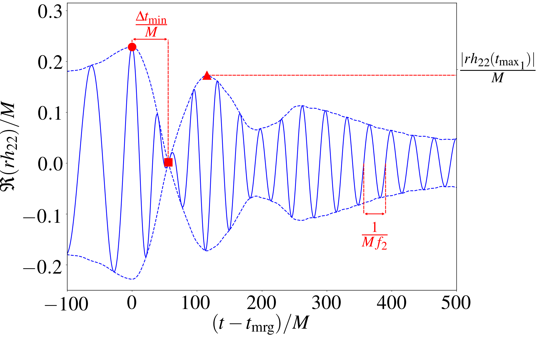
Figure 1: A typical time domain representation of a postmerger waveform (THC:0001 Dietrich et al. (2018); Radice et al. (2017, 2018)); cf. Tab. LABEL:tab:NR_data. As throughout the article, we restrict our considerations to the dominant 22-mode.

While the inspiral GW signal is characterized by a chirp, i.e., a monotonic increase of the GW amplitude and frequency, the postmerger emission shows a non-monotonic amplitude and frequency evolution. Figure 1 presents one example of a possible postmerger waveform. In the following, we highlight some of the important features characterizing the signal.

First postmerger minimum: By definition, the inspiral ends at the peak of the GW amplitude (merger) marked with a red circle in Fig. 1. After the merger, the amplitude decreases showing a clear minimum (red squared marker) shortly afterwards, see Thierfelder et al. (2011); Kastaun et al. (2017) for further discussions. Around this intermediate and highly non-linear regime, different frequencies are excited for a few milliseconds, see e.g., Bauswein and Stergioulas (2015); Rezzolla and Takami (2016) for further details. While it was already known that the merger frequency can be expressed by a quasi-universal relation, e.g., Takami et al. (2014); Bernuzzi et al. (2014), we find that the time between merger and this amplitude minimum also follows a similar relation.

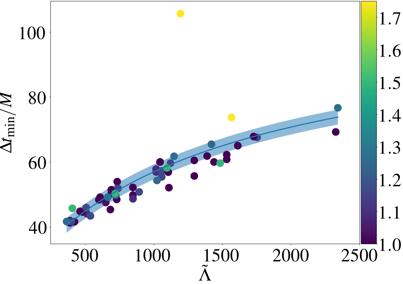
Figure 2: Dimensionless time between the merger and the first amplitude minimum within the postmerger as a function of the mass-weighted tidal deformability $\tilde{\Lambda}$. The color shows the mass ratio $q$. The shaded region indicates the 1-sigma ($\pm 2.2913$) uncertainty.

In Fig. 2 we show the time between the merger and the first amplitude minimum, $\Delta t_{\rm min}/M$, as a function of the mass-weighted tidal deformability

$$\tilde{\Lambda}=\frac{16}{13}\frac{(M_{A}+12M_{B})M_{A}^{4}\Lambda_{A}+(M_{B}+12M_{A})M_{B}^{4}\Lambda_{B}}{(M_{A}+M_{B})^{5}}\,.$$ (1)

with the individual dimensionless tidal deformabilities $\Lambda=\frac{2}{3}k_{2}(\frac{R}{M})^{5}$, where $k_{2}$ labels the dimensionless $\ell=2$ Love number and $R$ labels the radius of the isolated NSs. We show with different colors the mass ratio of each setup defined as $q=M_{A}/M_{B}\geqslant 1$, cf. colorbar of Fig. 2.

We find a clear correlation between $\Delta t_{\rm min}/M$ and the mass-weighted tidal deformability $\tilde{\Lambda}$. A good phenomenological representation is given by

$$\frac{\Delta t_{\rm min}}{M}=\alpha\frac{1+\beta\tilde{\Lambda}}{1+\gamma\tilde{\Lambda}},$$ (2)

with the parameters $\alpha=2.4681\times 10^{1},\beta=2.8477\times 10^{-3},\gamma=6.6798\times 10^{-4}$ obtained by a least-square fit for which the root-mean-square (RMS) error is $2.4608$. Interestingly, the two highest mass ratio simulations do not follow Eq. (2). This is caused by the different postmerger evolution for these high-mass ratio setups. While the amplitude minimum is produced when the two NS cores approach each other and potentially get repelled, configurations with very high mass ratio show almost a disruption during the merger, i.e., the lower massive NS deforms significantly under the strong external gravitational field of its companion.

One possible application for the quasi-universal relation for $\Delta t_{\rm min}/M$ is the improvement of BNS waveform approximants, i.e., it might help to determine the amplitude evolution after the merger of the two NSs. In particular, incorporating an amplitude tapering after the merger with a width of $\Delta t_{\rm min}$ provides a natural ending condition for inspiral-only approximants, e.g., NRTidal Dietrich et al. (2017); Dietrich et al. (2019a, b) or tidal effective-one-body models Bernuzzi et al. (2015b); Hinderer et al. (2016); Nagar et al. (2018). Therefore, Eq. (2) might become a central criterion to connect inspiral and postmerger models.

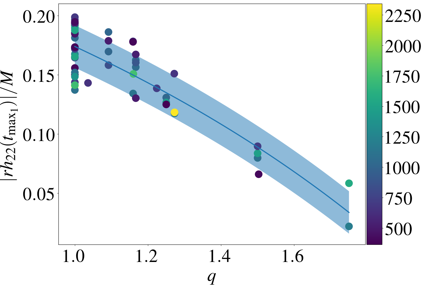
Figure 3: A scatter plot of the first peak in the postmerger spectra after merger versus $q$. The color shows the mass-weighted tidal deformability $\tilde{\Lambda}$. The shaded region indicates the 1-sigma ($\pm 1.7915\times 10^{-2}$) uncertainty.

First postmerger maximum: After the minimum of the GW amplitude, the amplitude grows and reaches a maximum, marked with a red diamond in Fig. 1. One finds that the main binary property determining the amplitude of this first postmerger GW amplitude maximum is the mass ratio of the binary $q$, cf. Fig. 3 with

$$\dfrac{|rh_{\rm 22}(t_{\rm{max}_{1}})|}{M}=(2.8437\times 10^{-1})\frac{1-(5.3149\times 10^{-1})q}{1-(2.3420\times 10^{-1})q}.$$ (3)

The qualitative behavior is again related to the possible tidal disruption of the binary close to the merger for unequal mass systems. We note that even if the secondary star does not get disrupted, the maximum density in the remnant shows one peak rather than two independent cores Kastaun et al. (2016); Hanauske et al. (2019) which leads to a smaller first postmerger peak and overall on average a smaller GW amplitude.

II.2 Frequency domain

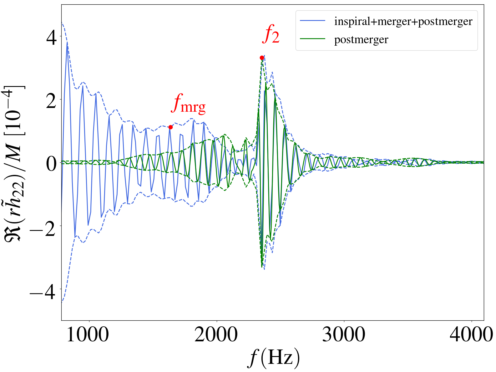
Figure 4: Frequency domain gravitational waveform (for the dominant 22 mode) for the setup THC:0001. In blue we show the FFT of the time domain waveform shown in Fig. 1, while in green we show only the postmerger part obtained by discarding the inspiral signal in the time domain. The two marked characteristic frequencies are the merger frequency $f_{\rm mrg}$ and the main postmerger emission frequency $f_{2}$.

We obtain the frequency domain waveform by fast Fourier transformation (FFT) of the time domain GW strain $h(t)$:

$$\tilde{h}(f)=\int^{\infty}_{-\infty}h(t)e^{-i2\pi ft}\differential t.$$ (4)

As before, we consider only the dominant 22-mode of the GW signal.

In Fig. 4 we show the frequency domain GW signal (blue solid line) of THC:0001. The merger frequency of this particular configuration is 1638 Hz and it is marked with a red circle. The main feature of the postmerger spectrum is the dominant peak characterizing the main emission frequency $f_{2}$, which for the setup shown in the Figs. 1 and 4 is about 2354 Hz. For a better interpretation, we also present the frequency domain postmerger spectrum in green. Such postmerger-only waveforms are obtained by FFT after applying a Tukey window Harris (1978) with a shape parameter 0.05 at $t_{\rm min}$ (where the shape parameter represents the fraction of the window inside the cosine tapered region) and will be used for our injections to test our parameter estimation infrastructure.

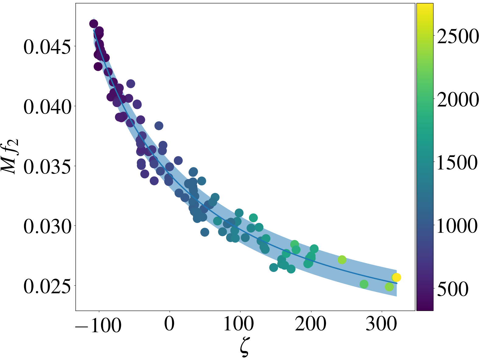
Figure 5: $Mf_{2}$ as a function of $\zeta$. The color shows the mass-weighted tidal deformability $\tilde{\Lambda}$. The shaded region indicates the 1-sigma ($\pm 1.1025\times 10^{-3}$) uncertainty. In addition to the CoRe-dataset employed to derive the previously shown quasi-universal relations, we include here the published results of Takami et al. (2015); Hotokezaka et al. (2013).

$f_{2}$-frequency: The dominant feature in the postmerger frequency spectrum is the dominant emission mode of the merger remnant at a frequency $f_{2}$. As mentioned before, a number of works, e.g., Bauswein and Janka (2012); Clark et al. (2014); Takami et al. (2014); Bernuzzi et al. (2015a); Rezzolla and Takami (2016) have discussed possible EOS-insensitive, quasi-universal relation for the $f_{2}$-frequency.

Building mostly on the work of Bernuzzi et al. Bernuzzi et al. (2015a), we derive a new relation for the $f_{2}$ frequency. First, we extend the dataset of 99 NR simulations employed in Ref. Bernuzzi et al. (2015a) and use a set of 121 data by incorporating additional setups published as a part of the CoRe database Dietrich et al. (2018); cf. Tab. LABEL:tab:NR_data. Second, we are switching from

$$\kappa^{\rm T}_{2}\equiv 2\left[\dfrac{1}{q}\left(\dfrac{X_{A}}{C_{A}}\right)^{5}k^{A}_{2}+q\left(\dfrac{X_{B}}{C_{B}}\right)^{5}k^{B}_{2}\right],$$ (5)

to

$$\kappa^{\rm T}_{\rm eff}\equiv\frac{2}{13}\left[\left(1+12\frac{X_{B}}{X_{A}}\right)\left(\frac{X_{A}}{C_{A}}\right)^{5}k^{A}_{2}+(A\leftrightarrow B)\right]\ =\frac{3}{16}\tilde{\Lambda}$$ (6)

which yields a tiny improvement ($\sim 0.1\%$) in the RMS error against the NR data, but more notably relates directly to the mass-weighted tidal deformability $\tilde{\Lambda}$ measured most accurately from the inspiral part of the signal. In addition to the dependence of the mass-weighted tidal deformability $\tilde{\Lambda}$, the postmerger evolution depends also on the stability of the formed remnant and how close it is to the black hole formation. This information is in part encoded in the ratio between the total mass $M$ and the maximum allowed mass of a single non-rotating NS $M_{\mathrm{TOV}}$. By incorporating an additional $M/M_{\rm TOV}$ dependence we are able to reduce the RMS error by $\approx 28\%$.

Therefore, we define a parameter $\zeta$ by a linear combination of $\kappa_{\mathrm{eff}}^{\rm T}$ and $\frac{M}{M_{\mathrm{TOV}}}$ (see also Coughlin et al. (2018); Zappa et al. (2019, 2018b) for a similar approach),

$$\zeta=\kappa_{\mathrm{eff}}^{\rm T}+a\dfrac{M}{M_{\mathrm{TOV}}}.$$ (7)

The free parameter $a=-131.7010$ is determined by minimizing the RMS error. Finally, the dimensionless frequency $Mf_{2}$ is fitted against $\zeta$ using a Padé approximant:

$$Mf_{2}(\zeta)=\alpha\dfrac{1+A\zeta}{1+B\zeta}$$ (8)

with $\alpha=3.4285\times 10^{-2}$, $A=2.0796\times 10^{-3}$ and $B=3.9588\times 10^{-3}$. We present Eq. (8) together with our NR dataset and a one sigma uncertainty region (shaded area) in Fig. 5.

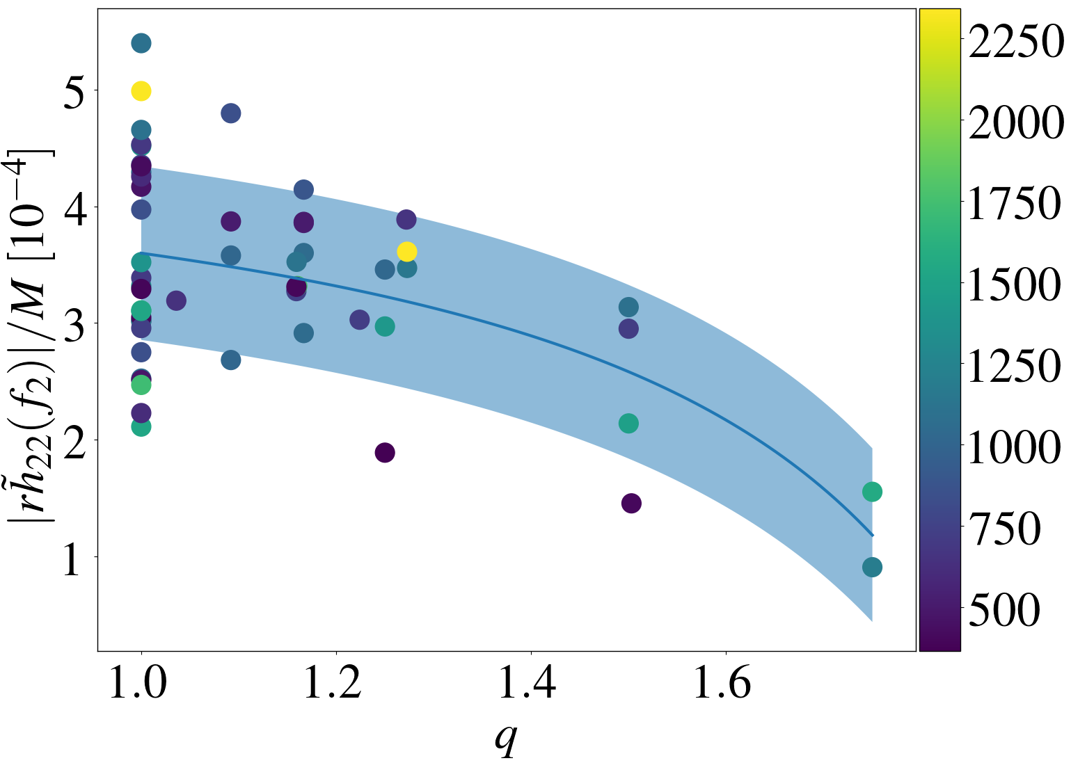
Figure 6: $|r\tilde{h_{\rm 22}}(f_{2})/M|$ as a function of the mass ratio $q$ with 1-sigma ($\pm 7.4485\times 10^{-5}$) shaded region. The color shows the tidal deformability $\tilde{\Lambda}$.

Frequency domain amplitude of $f_{2}$: Finally, we want to briefly discuss the dependence of the $f_{2}$-peak amplitude on the binary properties. While the $f_{2}$-frequency correlates clearly to $\zeta$, we have not been able to find a similar tight relation between any combination of the binary parameters and the amplitude $|\tilde{h}_{\rm 22}(f_{2})|$. The only noticeably imprint which we have been able to extract comes from the mass ratio $q$, where generally higher mass ratios lead to a smaller amplitude $|r\tilde{h}_{\rm 22}(f_{2})/M|$ as shown in Fig. 6 with

$$\dfrac{|r\tilde{h}_{\rm 22}(f_{2})|}{M}=(4.2319\times 10^{-4})\frac{1-(5.4016\times 10^{-1})q}{1-(4.5927\times 10^{-1})q}.$$ (9)

We note that because of the large uncertainty, we see Eq. (9) more as a qualitative rather than a quantitative statement about the postmerger spectrum. However, the overall amplitude decreases for an increasing mass ratio seems to be a robust feature and might help to interpret future GW observations.

III Model functions, $f_{2}$ measurement, and inspiral-postmerger consistency

III.1 Lorentzian Approximants

Based on our previous discussion and the dominance of the characteristic $f_{2}$ frequency, we start our consideration with a simple damped sinusoidal time domain waveform to model the postmerger waveform. The Fourier transform of a damped sinusoidal function is a Lorentzian function, Eq. (10). In the simplest case which we consider, we use 3 unknown coefficients ($c_{0},c_{1},c_{2}$) corresponding to the amplitude, the dominant emission frequency and the inverse of the damping time, respectively, and write the frequency-domain signal as:

$$\tilde{h}_{22}(f)=\dfrac{c_{0}\ c_{2}}{\sqrt{(f-c_{1})^{2}+c_{2}^{2}}}e^{-i\arctan(\frac{f-c_{1}}{c_{2}})}.$$ (10)

Equation (10) suggests that the amplitude peak of the GW postmerger spectrum and also the main postmerger phase evolution are connected to the same frequency characterized by $c_{1}$.

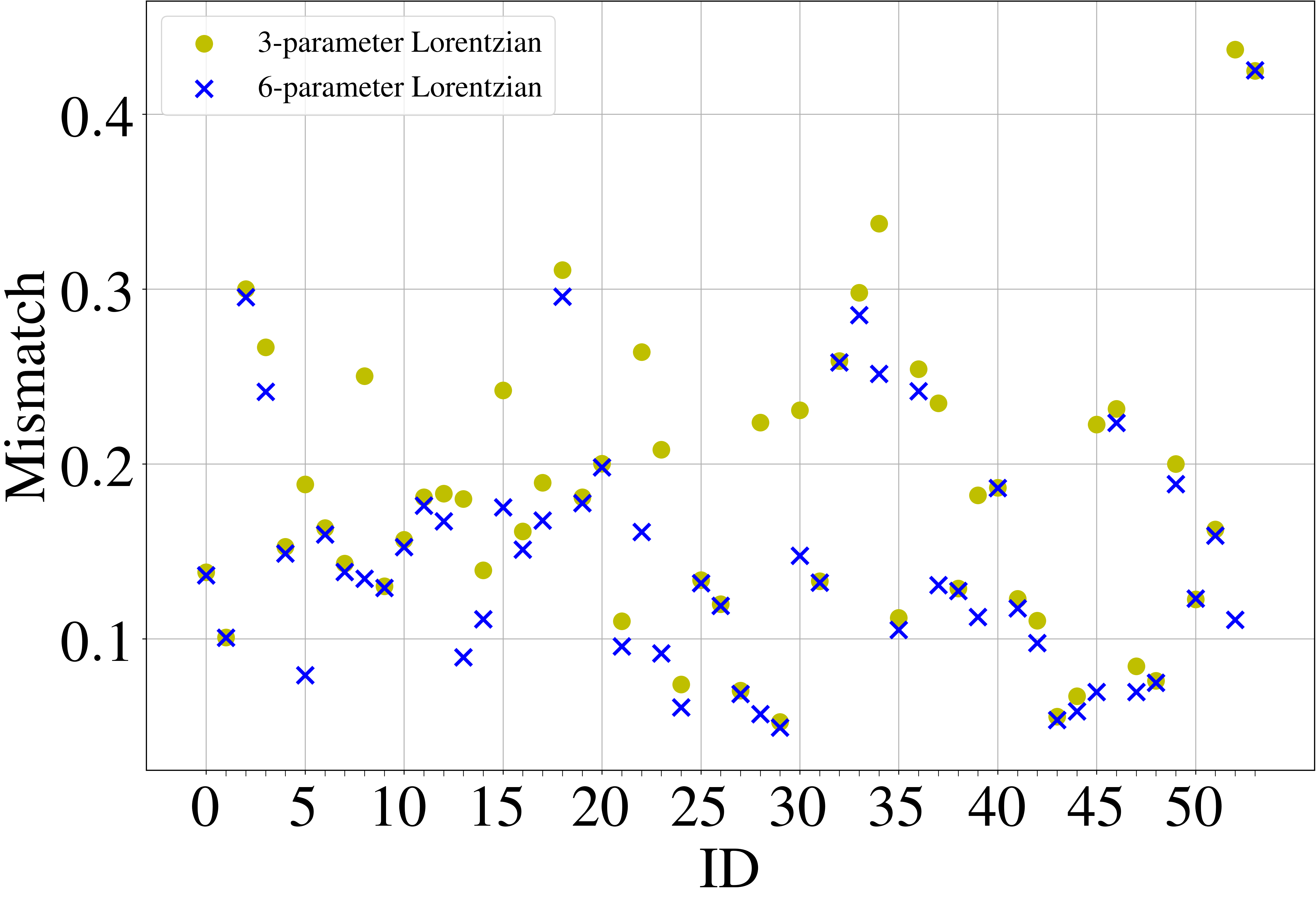
Figure 7: Mismatch between a subset of the NR data listed in Tab. LABEL:tab:NR_data and the three- and six-parameter models.

Maximizing over ($c_{0},c_{1},c_{2}$), we compute the mismatches between the used NR data from the CoRe-database (Tab. LABEL:tab:NR_data) and the model function, Eq. (10). Figure 7 shows all mismatches, which on average are $\sim 0.18$.

The mismatches can be further decreased by adding three additional coefficients:

$$\tilde{h}_{22}(f)=\dfrac{c_{0}\ c_{2}}{\sqrt{(f-c_{1})^{2}+c_{2}^{2}}}e^{-ic_{3}\arctan(\frac{f-c_{5}}{c_{4}})}.$$ (11)

For Eq. (11) the amplitude and phase evolution are independent from each other and we obtain average mismatches of $0.15$, i.e., about $17\%$ better than for the three-parameter model. While one might argue that the additional introduced degrees of freedom hinder the extraction of individual parameters in a full Bayesian analysis, it might also be possible that the more flexible 6-parameter model recovers signals with smaller SNRs. Thus, we continue our study with both model functions Eqs. (10) and (11).

Finally, one obtains the plus and cross polarizations from Eq. (10) and Eq. (11) by incorporating the inclination ($\iota$) dependence:

$$\tilde{h}_{p} =\dfrac{1+\cos^{2}(\iota)}{2}\tilde{h}_{22},$$ (12)

$$\tilde{h}_{c} =-i\cos(\iota)\tilde{h}_{22}.$$ (13)

$\tilde{h}_{c},\tilde{h}_{p}$ can be employed directly to infer information from the postmerger part of a GW signal or to construct a full IMP-waveform for BNSs.

III.2 Validating the Parameter Estimation Pipeline

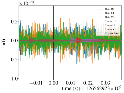
Figure 8: Injection of THC:0021 with SNR 8, zero inclination angle, zero polarization angle and sky location (0,0). Top panel: time domain signal of the postmerger waveform highlighted within the detectors noise for H1–Hanford, L1–Livingston, and V1–Virgo. Bottom panel: frequency domain signal and design amplitude spectral density (ASD) for H1, L1, and V1.

In this section, we present for four selected cases the performance of the three- and six-parameter models. We inject the NR waveforms immersed in the same simulated Gaussian noise with total network SNRs ranging from SNR 0 to SNR 10 assuming that Advanced LIGO and Advanced Virgo detectors run at design sensitivity Abbott et al. (2018c) . Fig. 8 shows the injection of THC:0021 with SNR 8 in both the time (top panel) and frequency domain (bottom panel). For each injected waveform, a Tukey window with shape parameter 0.05 is applied at $t_{\rm min}$ to isolate the postmerger signal and avoid Gibbs phenomenon. All simulated signals are injected with zero inclination angle, zero polarization angle $\psi$ and sky location ($\alpha,\delta$) to be ($0,0$).

We estimate parameters using Bayesian inference with the LALInference module Veitch et al. (2015) available in the LALSuite package. Sampling is done on 9 (12) parameters

$$\{c_{i},\alpha,\delta,\iota,\psi,t_{c},\phi_{c}\}$$ (14)

with nested sampling algorithm lalinferencenest Veitch and Vecchio (2010), where $i$ runs from 0 to 2 (5) for the three- (six-) parameter model, and $t_{c}$ and $\phi_{c}$ are the reference time and phase, respectively. The priors are chosen to be uniform in $[0,10^{-20}]{\rm s^{-1}}$ on $c_{0}$, uniform in $[1500,4096]{\rm Hz}$ on $c_{1}$ and $c_{5}$, uniform in $[1,400]{\rm Hz}$ on $c_{2}$ and $c_{4}$, uniform in $[0,6]$ on $c_{3}$, uniform in $[0,2\pi]$ on $\alpha,\psi$ and $\phi_{c}$, uniform in $[-1,1]$ on $\cos(\iota)$ and $\sin(\delta)$, and uniform in $[{\rm trigger~{}time}-0.05{\rm s},{\rm trigger~{}time}+0.05{\rm s}]$ on $t_{c}$ where the trigger time is the signal arrival time at the geocentric frame.

Figure 9: Posteriors for the parameter $c_{1}$ in Eq. (10) (top panels) and Eq. (11) (bottom panels) for a variety of SNRs. $c_{1}$ can be directly related to the peak in the frequency domain spectrum and therefore relates to the $f_{2}$ frequency. The IDs of the four injected waveforms are # 18, 20, 32, 34, i.e., THC:0021, THC:0031, BAM:0048, BAM:0057 of Dietrich et al. (2018). The chosen set covers various EOSs, mass ratios, and masses and is therefore used as a testbed for our new algorithm.

Fig. 9 shows the posterior for $c_{1}$, i.e., our best estimate of the $f_{2}$-frequency for SNRs up to 8 for our 4 examples, which we mark in Tab. LABEL:tab:NR_data. We present the recovery with the 3- and the 6-parameter model in the top and bottom panels, respectively. The solid vertical line represents the injected $f_{2}$-frequency and the dashed line represents the estimate according to the quasi-universal relation Eq. (8) together with a one-sigma uncertainty (gray shaded region).

Figure 10: Posteriors for the parameter $c_{1}$ and $c_{5}$ in Eq. (11) for 2 SNRs. $c_{5}$ peaks at a frequency close to $f_{2}$ but it is significantly less constrained than $c_{1}$.

We summarize the main findings below:

1. The three-parameter and six-parameter approximants perform similarly.

2. Depending on the exact setting (e.g., intrinsic source properties, noise realization, sky location) one can recover the $f_{2}$ frequency with an SNR of $\sim 4$ for the best and $\sim 8$ for worst considered scenarios.

3. Interestingly, one finds that also $c_{5}$ relates to a frequency which is close to the $f_{2}$ frequency, however, $c_{5}$ is significantly less constrained than $c_{1}$ (Fig. 10).

4. Once 3rd generation detectors are available and so the postmerger SNRs of $\sim 10$ are obtained, the systematic uncertainties of the quasi-universal relations become larger than the statistical uncertainties; cf. dashed and solid, vertical black lines.

III.3 Inspiral and Postmerger consistency

Figure 11: Schematic plot showing how one can constrain $\zeta$ from $f_{2}$ measurements where the spread $f_{2}$ are measured by one standard deviation. Top panel is for three-parameter model and the bottom panel is for six-parameter model. The vertical red shaded region corresponds to the $\zeta$-interval consistent with a hypothetical inspiral signal assuming an uncertainty of $\pm 0.04M_{\odot}$ for $M$ and $M_{\rm TOV}$, and $\pm 30$ for $\kappa_{\rm eff}^{\rm T}$. The exact value is marked as vertical red-dashed line.

Finally, we want to illustrate how a future detection of a postmerger GW signal will help to constrain the source properties and the internal composition of NSs. As shown before, the $f_{2}$-frequency can be extracted through a simple waveform model (or alternatively by using BayesWave, e.g., Chatziioannou et al. (2017)). To connect the $f_{2}$-frequency with the source parameters, one needs to employ quasi-universal relations as presented in Sec. II and some information obtained from the analysis of the inspiral GW signal. In particular, the total mass $M$ can be measured precisely using state-of-art BNS inspiral waveforms, e.g., Damour et al. (2012); Dietrich et al. (2019a); Kawaguchi et al. (2018); Messina et al. (2019); Schmidt and Hinderer (2019); Dietrich et al. (2019b); Bernuzzi et al. (2015b); Hinderer et al. (2016); Nagar et al. (2018); Lackey et al. (2018); Lange et al. (2017, 2018). For GW170817 the uncertainty of $M$ could be reduced to $\pm 0.04M_{\odot}$ once EM information had been included Coughlin et al. (2018); Radice and Dai (2019). Thus, we will use an uncertainty of $\Delta M=\pm 0.04M_{\odot}$ as a conservative estimate. In addition, we have to know the maximum TOV-mass $M_{\rm TOV}$. Current estimates for $M_{\rm TOV}$ are based on the observation of J0740+6620 (Cromartie et al., 2019) with $M=2.17^{+0.11}_{-0.10}M_{\odot}$ and the assumption that GW170817’s endstate was a black hole Margalit and Metzger (2017); Rezzolla et al. (2018); Ruiz et al. (2018); Shibata et al. (2019) such that $M_{\rm TOV}\lesssim 2.17$-$2.35M_{\odot}$. Due to the increasing number of BNS detections in the future, we expect that the uncertainty of $M_{\rm TOV}$ can be considerably reduced so that we will use an uncertainty of $\pm 0.04M_{\odot}$. From this information, we can compute the $\zeta$-interval consistent with the observed inspiral signal from the $\tilde{\Lambda}$ posteriors, cf. vertical red shaded region in Fig. 11. We then connect the $\zeta$ estimate obtained from the inspiral with Eq. (8) and the $f_{2}$-measurement of the postmerger signal. This consistency analysis is somewhat connected to the inspiral-merger-ringdown consistency test for BBH Ghosh et al. (2018), but not only has to assume the correctness of general relativity but also that our understanding of supranuclear matter and the EOS-insensitive quasi-universal relations are valid.

Figure 11 summarizes our main results. Generally the GW measurements can be considered consistent between the inspiral and postmerger observations as well as with the quasi-universal relation relating the main postmerger frequency with the binary properties. We find that for all cases, the quasi-universal relation and its 1-sigma uncertainty region lie within the intersection of the red shaded region (inspiral) and the blue/orange/green horizontal regions (postmerger). Thus, (as expected) all simulations are consistent with (i) general relativity and (ii) the nuclear physics descriptions used as a basis for NR simulations to derive the quasi-universal relations. For future events this approach will allow us to probe our understanding of physical processes under extreme conditions, and in cases where the quasi-universal relation seems violated to even derive new relations based on GW measurements (under the assumption that general relativity is correct). We note that even in the case where either general relativity or the quasi-universal relations would be violated, we might not be able to determine reliably the violation based on one individual event, but stronger constraints can be obtained by combining multiple BNS events.

IV Summary

In this work, we discussed the general morphology of a BNS postmerger in both the time and frequency domain. We presented quasi-universal relations for the time at which the first postmerger amplitude minimum happens and the strength of the first postmerger amplitude maximum. In general, the time between the merger and the amplitude minimum increases with an increasing $\tilde{\Lambda}$, while the amplitude of the first postmerger maximum decreases with an increasing mass ratio. In the frequency domain, we improved the existing quasi-universal relations of $Mf_{2}$ by extending the employed NR dataset (121 simulations in total) and adding an extra dependence of $M/M_{\rm TOV}$. The extra term $M/M_{\rm TOV}$ characterizes how close the setup is to the black hole formation.

We find that a three- (six-) parameter Lorentzian can model the postmerger waveform with average mismatch of 0.18 (0.15). To test these model functions, we performed an injection study, in which we simulated the detector strains with four different BNS configurations immersed in the same simulated Gaussian noise assuming Advanced LIGO and Advanced Virgo at design sensitivities. We find that in the best cases the Lorentzian models could measure the dominant emission frequency $f_{2}$ once the signal has an SNR of 4 or above; however, for most scenarios higher SNRs $\sim 8$ were required.

Employing the new quasi-universal relation for $Mf_{2}$ described in this work, we could present consistency tests between the inspiral and the postmerger signal; cf. Fig. 11.

Appendix A NR configurations

ID	Code/CoRe-ID	EOS	$\mathrm{M}_{\mathrm{TOV}}$ [$\mathrm{M_{\odot}}$]	M [$\mathrm{M_{\odot}}$]	q	$\kappa_{\mathrm{eff}}^{\rm T}$	$\dfrac{\Delta t_{\mathrm{min}}}{M}$	$\dfrac{|rh_{22}(t_{\mathrm{{max}_{1}}})|}{M}[10^{-2}]$	$f_{2}(\mathrm{Hz})$	$\dfrac{|r\tilde{h}_{22}(f_{2})|}{M}[10^{-4}]$
#0	THC:0001	BHBlp	2.10	2.50	1.00	242	55.68	17.27	2354	3.32
#1	THC:0002	BHBlp	2.10	2.60	1.00	196	60.00	19.20	2458	4.29
#2	THC:0003	BHBlp	2.10	2.70	1.00	159	49.78	19.65	2726	3.97
#3	THC:0004	BHBlp	2.10	2.62	1.09	190	56.90	18.62	2602	3.58
#4	THC:0005	BHBlp	2.10	2.60	1.17	198	55.38	16.24	2478	3.60
#5	THC:0006	BHBlp	2.10	2.80	1.00	129	51.43	18.57	2912	3.01
#6	THC:0007	BHBlp	2.10	2.83	1.04	121	47.49	14.32	2767	3.19
#7	THC:0010	DD2	2.42	2.40	1.00	302	65.00	19.15	2231	3.11
#8	THC:0011	DD2	2.42	2.50	1.00	242	60.48	16.75	2354	3.02
#9	THC:0012	DD2	2.42	2.60	1.00	196	60.00	18.13	2478	2.52
#10	THC:0013	DD2	2.42	2.70	1.00	159	52.15	16.45	2664	2.75
#11	THC:0014	DD2	2.42	2.62	1.09	190	57.82	16.97	2437	2.68
#12	THC:0015	DD2	2.42	2.60	1.17	198	57.23	15.65	2478	2.91
#13	THC:0016	DD2	2.42	2.80	1.00	129	50.29	14.37	2571	3.39
#14	THC:0017	DD2	2.42	3.00	1.00	86	44.80	15.01	2767	4.17
#15	THC:0018	LS220	2.04	2.40	1.00	269	60.00	18.96	2520	4.52
#16	THC:0019	LS220	2.04	2.70	1.00	128	45.33	19.88	3015	4.53
#17	THC:0020	LS220	2.04	2.62	1.09	159	48.64	15.82	2850	4.80
#18	THC:0021	LS220	2.04	2.60	1.17	167	50.77	16.04	2726	4.14
#19	THC:0029	MS1b	2.76	2.70	1.00	287	60.80	16.53	2014	2.11
#20	THC:0031	SFHo	2.06	2.62	1.09	96	44.05	17.88	3222	3.87
#21	THC:0032	SFHo	2.06	2.60	1.17	100	43.38	16.73	3056	3.86
#22	THC:0036	SLy	2.06	2.70	1.00	73	41.24	15.58	3459	3.05
#23	BAM:0002	2H	2.83	2.70	1.00	436	69.25	14.09	1871	4.99
#24	BAM:0003	ALF2	1.99	2.70	1.00	137	53.94	17.20	2720	2.96
#25	BAM:0004	ALF2	1.99	2.70	1.00	136	48.45	19.38	2791	4.36
#26	BAM:0009	ALF2	1.99	2.50	1.27	215	61.75	11.74	2391	3.47
#27	BAM:0010	ALF2	1.99	2.70	1.16	138	51.85	17.83	2633	3.27
#28	BAM:0022	ENG	2.25	2.70	1.00	89	44.59	18.48	2933	2.51
#29	BAM:0035	H4	2.03	2.70	1.00	208	52.08	13.72	2406	4.66
#30	BAM:0036	H4	2.03	2.70	1.00	207	56.85	15.20	2526	5.40
#31	BAM:0046	H4	2.03	2.70	1.16	210	59.62	13.42	2344	3.52
#32	BAM:0048	H4	2.03	2.75	1.25	191	54.30	13.08	2416	3.46
#33	BAM:0053	H4	2.03	2.75	1.50	205	58.18	7.98	2471	3.14
#34	BAM:0057	H4	2.03	2.75	1.75	223	105.69	2.19	2490	0.90
#35	BAM:0058	MPA1	2.47	2.70	1.00	114	49.16	19.34	2720	2.23
#36	BAM:0059	MS1	2.77	2.70	1.16	328	67.56	15.08	2065	3.32
#37	BAM:0061	MS1	2.77	2.70	1.00	323	67.84	14.13	2013	2.47
#38	BAM:0065	MS1b	2.76	2.70	1.00	287	62.25	18.77	2043	3.10
#39	BAM:0070	MS1b	2.76	2.75	1.00	260	61.82	14.85	2120	3.52
#40	BAM:0080	MS1b	2.76	2.50	1.27	439	76.67	11.83	2084	3.61
#41	BAM:0089	MS1b	2.76	2.75	1.25	266	65.45	12.67	2067	2.97
#42	BAM:0090	MS1b	2.76	3.20	1.00	112	48.33	17.35	2306	4.26
#43	BAM:0091	MS1b	2.76	2.75	1.50	278	59.63	8.37	1956	2.14
#44	BAM:0092	MS1b	2.76	3.40	1.00	79	41.57	19.48	2433	4.34
#45	BAM:0093	MS1b	2.76	2.75	1.75	293	73.70	5.84	1970	1.55
#46	BAM:0098	SLy	2.06	2.70	1.00	73	41.88	17.33	3340	3.29
#47	BAM:0107	SLy	2.06	2.46	1.22	135	49.78	13.86	2784	3.03
#48	BAM:0121	SLy	2.06	2.50	1.27	124	49.16	15.10	2787	3.89
#49	BAM:0122	SLy	2.06	2.60	1.17	95	45.95	13.03	3050	3.87
#50	BAM:0123	SLy	2.06	2.70	1.16	74	41.61	17.79	3362	3.31
#51	BAM:0124	SLy	2.06	2.50	1.50	134	50.27	8.96	2951	2.95
#52	BAM:0126	SLy	2.06	2.75	1.25	68	41.66	12.50	3460	1.89
#53	BAM:0128	SLy	2.06	2.75	1.50	76	45.73	6.60	3339	1.45
#54	whisky	Gamma2	1.82	2.90	1.00	277	-	-	2127	-
#55	whisky	Gamma2	1.82	2.85	1.00	324	-	-	2183	-
#56	whisky	Gamma2	1.82	2.80	1.00	379	-	-	2061	-
#57	whisky	Gamma2	1.82	2.75	1.00	442	-	-	2004	-
#58	whisky	Gamma2	1.82	2.70	1.00	516	-	-	1930	-
#59	whisky	GNH3	1.98	2.50	1.00	345	-	-	2272	-
#60	whisky	GNH3	1.98	2.55	1.00	306	-	-	2302	-
#61	whisky	GNH3	1.98	2.60	1.00	271	-	-	2425	-
#62	whisky	GNH3	1.98	2.65	1.00	240	-	-	2479	-
#63	whisky	GNH3	1.98	2.70	1.00	213	-	-	2595	-
#64	whisky	ALF2	1.99	2.45	1.00	236	-	-	2443	-
#65	whisky	ALF2	1.99	2.50	1.00	212	-	-	2493	-
#66	whisky	ALF2	1.99	2.55	1.00	190	-	-	2574	-
#67	whisky	ALF2	1.99	2.60	1.00	170	-	-	2655	-
#68	whisky	ALF2	1.99	2.65	1.00	153	-	-	2693	-
#69	whisky	H4	2.03	2.50	1.00	327	-	-	2247	-
#70	whisky	H4	2.03	2.55	1.00	292	-	-	2377	-
#71	whisky	H4	2.03	2.60	1.00	260	-	-	2356	-
#72	whisky	H4	2.03	2.65	1.00	232	-	-	2449	-
#73	whisky	H4	2.03	2.70	1.00	208	-	-	2501	-
#74	whisky	SLy	2.06	2.50	1.00	118	-	-	3154	-
#75	whisky	SLy	2.06	2.55	1.00	105	-	-	3235	-
#76	whisky	SLy	2.06	2.60	1.00	93	-	-	3229	-
#77	whisky	SLy	2.06	2.65	1.00	82	-	-	3282	-
#78	whisky	SLy	2.06	2.70	1.00	73	-	-	3338	-
#79	whisky	SLy	2.06	2.60	1.08	93	-	-	3212	-
#80	whisky	APR4	2.20	2.55	1.00	85	-	-	3229	-
#81	whisky	APR4	2.20	2.60	1.00	75	-	-	3279	-
#82	whisky	APR4	2.20	2.65	1.00	67	-	-	3373	-
#83	whisky	APR4	2.20	2.70	1.00	60	-	-	3462	-
#84	sacra	APR4	2.20	2.70	1.00	60	-	-	3450	-
#85	sacra	APR4	2.20	2.70	1.00	60	-	-	3255	-
#86	sacra	APR4	2.20	2.70	1.00	60	-	-	3330	-
#87	sacra	APR4	2.20	2.60	1.00	76	-	-	3210	-
#88	sacra	SLy	2.06	2.70	1.25	76	-	-	3340	-
#89	sacra	SLy	2.06	2.70	1.16	74	-	-	3320	-
#90	sacra	SLy	2.06	2.70	1.08	73	-	-	3390	-
#91	sacra	SLy	2.06	2.70	1.00	73	-	-	3480	-
#92	sacra	SLy	2.06	2.60	1.00	93	-	-	3160	-
#93	sacra	ALF2	1.99	2.80	1.00	110	-	-	2920	-
#94	sacra	ALF2	1.99	2.70	1.25	139	-	-	2820	-
#95	sacra	ALF2	1.99	2.70	1.16	138	-	-	2650	-
#96	sacra	ALF2	1.99	2.70	1.08	137	-	-	2770	-
#97	sacra	ALF2	1.99	2.70	1.00	137	-	-	2770	-
#98	sacra	ALF2	1.99	2.60	1.00	170	-	-	2630	-
#99	sacra	H4	2.03	2.90	1.00	133	-	-	2930	-
#100	sacra	H4	2.03	2.80	1.15	168	-	-	2505	-
#101	sacra	H4	2.03	2.80	1.00	166	-	-	2780	-
#102	sacra	H4	2.03	2.70	1.25	214	-	-	2320	-
#103	sacra	H4	2.03	2.70	1.25	214	-	-	2340	-
#104	sacra	H4	2.03	2.70	1.25	214	-	-	2300	-
#105	sacra	H4	2.03	2.70	1.16	210	-	-	2440	-
#106	sacra	H4	2.03	2.70	1.08	208	-	-	2475	-
#107	sacra	H4	2.03	2.70	1.00	208	-	-	2590	-
#108	sacra	H4	2.03	2.70	1.00	208	-	-	2530	-
#109	sacra	H4	2.03	2.70	1.00	208	-	-	2490	-
#110	sacra	H4	2.03	2.60	1.17	264	-	-	2370	-
#111	sacra	H4	2.03	2.60	1.08	261	-	-	2260	-
#112	sacra	H4	2.03	2.60	1.00	260	-	-	2310	-
#113	sacra	MS1	2.77	2.90	1.23	224	-	-	2120	-
#114	sacra	MS1	2.77	2.90	1.00	219	-	-	2110	-
#115	sacra	MS1	2.77	2.80	1.00	266	-	-	2045	-
#116	sacra	MS1	2.77	2.70	1.25	332	-	-	2110	-
#117	sacra	MS1	2.77	2.70	1.16	328	-	-	2050	-
#118	sacra	MS1	2.77	2.70	1.08	326	-	-	2050	-
#119	sacra	MS1	2.77	2.70	1.00	325	-	-	2020	-
#120	sacra	MS1	2.77	2.60	1.00	398	-	-	1960	-

Table 1: All NR configurations employed to derive the quasi-universal relations. It includes simulations of the CoRe database Dietrich et al. (2018) labeled as ‘THC’ or ‘BAM’, and additionally results published in Takami et al. (2015) labeled as ‘whisky’ and Hotokezaka et al. (2013) labeled as ‘sacra’. We highlight the simulations which have been used for the injection study discussed in the main text. The individual columns refer to: the number of simulation, the employed code, the EOS, the maximum TOV mass for the employed EOS, the total mass of the system, the mass ratio, the effective tidal coupling constant, the time at which the first postmerger minimum appears, the amplitude of the first postmerger maximum, the $f_{2}$ frequency, and the amplitude of the $f_{2}$ frequency peak.

References

- Aasi et al. (2015) J. Aasi et al. (LIGO Scientific), Class. Quant. Grav. 32, 074001 (2015), eprint 1411.4547.
- Acernese et al. (2015) F. Acernese et al. (VIRGO), Class. Quant. Grav. 32, 024001 (2015), eprint 1408.3978.
- Abbott et al. (2017a) B. P. Abbott et al. (LIGO Scientific, Virgo), Phys. Rev. Lett. 119, 161101 (2017a), eprint 1710.05832.
- Abbott et al. (2019) B. P. Abbott et al. (LIGO Scientific, Virgo), Phys. Rev. X9, 011001 (2019), eprint 1805.11579.
- Abbott et al. (2018a) B. P. Abbott et al. (LIGO Scientific, Virgo), Phys. Rev. Lett. 121, 161101 (2018a), eprint 1805.11581.
- Abbott et al. (2018b) B. P. Abbott et al. (LIGO Scientific, Virgo) (2018b), eprint 1811.12907.
- De et al. (2018) S. De, D. Finstad, J. M. Lattimer, D. A. Brown, E. Berger, and C. M. Biwer, Phys. Rev. Lett. 121, 091102 (2018), [Erratum: Phys. Rev. Lett.121,no.25,259902(2018)], eprint 1804.08583.
- Abbott et al. (2018c) B. P. Abbott et al. (KAGRA, LIGO Scientific, VIRGO), Living Rev. Rel. 21, 3 (2018c), eprint 1304.0670.
- Hinderer et al. (2010) T. Hinderer, B. D. Lackey, R. N. Lang, and J. S. Read, Phys. Rev. D81, 123016 (2010), eprint 0911.3535.
- Damour et al. (2012) T. Damour, A. Nagar, and L. Villain, Phys. Rev. D85, 123007 (2012), eprint 1203.4352.
- Del Pozzo et al. (2013) W. Del Pozzo, T. G. F. Li, M. Agathos, C. Van Den Broeck, and S. Vitale, Phys. Rev. Lett. 111, 071101 (2013), eprint 1307.8338.
- Lackey and Wade (2015) B. D. Lackey and L. Wade, Phys. Rev. D91, 043002 (2015), eprint 1410.8866.
- Agathos et al. (2015) M. Agathos, J. Meidam, W. Del Pozzo, T. G. F. Li, M. Tompitak, J. Veitch, S. Vitale, and C. Van Den Broeck, Phys. Rev. D92, 023012 (2015), eprint 1503.05405.
- Dietrich et al. (2019a) T. Dietrich et al., Phys. Rev. D99, 024029 (2019a), eprint 1804.02235.
- Kawaguchi et al. (2018) K. Kawaguchi, K. Kiuchi, K. Kyutoku, Y. Sekiguchi, M. Shibata, and K. Taniguchi, Phys. Rev. D97, 044044 (2018), eprint 1802.06518.
- Hinderer (2008) T. Hinderer, Astrophys. J. 677, 1216 (2008), eprint 0711.2420.
- Damour and Nagar (2010) T. Damour and A. Nagar, Phys. Rev. D81, 084016 (2010), eprint 0911.5041.
- Bauswein and Janka (2012) A. Bauswein and H. T. Janka, Phys. Rev. Lett. 108, 011101 (2012), eprint 1106.1616.
- Clark et al. (2014) J. Clark, A. Bauswein, L. Cadonati, H. T. Janka, C. Pankow, and N. Stergioulas, Phys. Rev. D90, 062004 (2014), eprint 1406.5444.
- Takami et al. (2014) K. Takami, L. Rezzolla, and L. Baiotti, Phys. Rev. Lett. 113, 091104 (2014), eprint 1403.5672.
- Rezzolla and Takami (2016) L. Rezzolla and K. Takami, Phys. Rev. D93, 124051 (2016), eprint 1604.00246.
- Bernuzzi et al. (2015a) S. Bernuzzi, T. Dietrich, and A. Nagar, Phys. Rev. Lett. 115, 091101 (2015a), eprint 1504.01764.
- Radice et al. (2017) D. Radice, S. Bernuzzi, W. Del Pozzo, L. F. Roberts, and C. D. Ott, Astrophys. J. 842, L10 (2017), eprint 1612.06429.
- Bauswein et al. (2019) A. Bauswein, N.-U. F. Bastian, D. B. Blaschke, K. Chatziioannou, J. A. Clark, T. Fischer, and M. Oertel, Phys. Rev. Lett. 122, 061102 (2019), eprint 1809.01116.
- Most et al. (2019) E. R. Most, L. J. Papenfort, V. Dexheimer, M. Hanauske, S. Schramm, H. Stöcker, and L. Rezzolla, Phys. Rev. Lett. 122, 061101 (2019), eprint 1807.03684.
- Bauswein et al. (2013) A. Bauswein, T. W. Baumgarte, and H. T. Janka, Phys. Rev. Lett. 111, 131101 (2013), eprint 1307.5191.
- Köppel et al. (2019) S. Köppel, L. Bovard, and L. Rezzolla, Astrophys. J. 872, L16 (2019), eprint 1901.09977.
- Bernuzzi et al. (2016) S. Bernuzzi, D. Radice, C. D. Ott, L. F. Roberts, P. Moesta, and F. Galeazzi, Phys. Rev. D94, 024023 (2016), eprint 1512.06397.
- Zappa et al. (2018a) F. Zappa, S. Bernuzzi, D. Radice, A. Perego, and T. Dietrich, Phys. Rev. Lett. 120, 111101 (2018a), eprint 1712.04267.
- Bauswein et al. (2012) A. Bauswein, H. T. Janka, K. Hebeler, and A. Schwenk, Phys. Rev. D86, 063001 (2012), eprint 1204.1888.
- Hotokezaka et al. (2013) K. Hotokezaka, K. Kiuchi, K. Kyutoku, T. Muranushi, Y.-i. Sekiguchi, M. Shibata, and K. Taniguchi, Phys. Rev. D88, 044026 (2013), eprint 1307.5888.
- Bauswein et al. (2014) A. Bauswein, N. Stergioulas, and H. T. Janka, Phys. Rev. D90, 023002 (2014), eprint 1403.5301.
- Takami et al. (2015) K. Takami, L. Rezzolla, and L. Baiotti, Phys. Rev. D91, 064001 (2015), eprint 1412.3240.
- Bauswein and Stergioulas (2015) A. Bauswein and N. Stergioulas, Phys. Rev. D91, 124056 (2015), eprint 1502.03176.
- Bose et al. (2018) S. Bose, K. Chakravarti, L. Rezzolla, B. S. Sathyaprakash, and K. Takami, Phys. Rev. Lett. 120, 031102 (2018), eprint 1705.10850.
- Chatziioannou et al. (2017) K. Chatziioannou, J. A. Clark, A. Bauswein, M. Millhouse, T. B. Littenberg, and N. Cornish, Phys. Rev. D96, 124035 (2017), eprint 1711.00040.
- Easter et al. (2018) P. J. Easter, P. D. Lasky, A. R. Casey, L. Rezzolla, and K. Takami (2018), eprint 1811.11183.
- Torres-Rivas et al. (2019) A. Torres-Rivas, K. Chatziioannou, A. Bauswein, and J. A. Clark, Phys. Rev. D99, 044014 (2019), eprint 1811.08931.
- Abbott et al. (2017b) B. P. Abbott et al. (LIGO Scientific, Virgo), Astrophys. J. 851, L16 (2017b), eprint 1710.09320.
- Abbott et al. (2018d) B. P. Abbott et al. (LIGO Scientific, Virgo) (2018d), eprint 1810.02581.
- Dudi et al. (2018) R. Dudi, F. Pannarale, T. Dietrich, M. Hannam, S. Bernuzzi, F. Ohme, and B. Bruegmann, Phys. Rev. D98, 084061 (2018), eprint 1808.09749.
- Hild et al. (2008) S. Hild, S. Chelkowski, and A. Freise (2008), eprint 0810.0Evans:2016mbw604.
- Punturo et al. (2010) M. Punturo et al., Class. Quant. Grav. 27, 194002 (2010).
- Ballmer and Mandic (2015) S. Ballmer and V. Mandic, Ann. Rev. Nucl. Part. Sci. 65, 555 (2015).
- Abbott et al. (2017c) B. P. Abbott et al. (LIGO Scientific), Class. Quant. Grav. 34, 044001 (2017c), eprint 1607.08697.
- Siegel et al. (2013) D. M. Siegel, R. Ciolfi, A. I. Harte, and L. Rezzolla, Phys. Rev. D87, 121302 (2013), eprint 1302.4368.
- Alford et al. (2018) M. G. Alford, L. Bovard, M. Hanauske, L. Rezzolla, and K. Schwenzer, Phys. Rev. Lett. 120, 041101 (2018), eprint 1707.09475.
- Radice (2017) D. Radice, Astrophys. J. 838, L2 (2017), eprint 1703.02046.
- Shibata and Kiuchi (2017) M. Shibata and K. Kiuchi, Phys. Rev. D95, 123003 (2017), eprint 1705.06142.
- De Pietri et al. (2018) R. De Pietri, A. Feo, J. A. Font, F. Löffler, F. Maione, M. Pasquali, and N. Stergioulas, Phys. Rev. Lett. 120, 221101 (2018), eprint 1802.03288.
- Clark et al. (2016) J. A. Clark, A. Bauswein, N. Stergioulas, and D. Shoemaker, Class. Quant. Grav. 33, 085003 (2016), eprint 1509.08522.
- (52) https://wiki.ligo.org/DASWG/LALSuite, URL https://wiki.ligo.org/DASWG/LALSuite.
- Veitch et al. (2015) J. Veitch et al., Phys. Rev. D91, 042003 (2015), eprint 1409.7215.
- Cornish and Littenberg (2015) N. J. Cornish and T. B. Littenberg, Class. Quant. Grav. 32, 135012 (2015), eprint 1410.3835.
- Bécsy et al. (2017) B. Bécsy, P. Raffai, N. J. Cornish, R. Essick, J. Kanner, E. Katsavounidis, T. B. Littenberg, M. Millhouse, and S. Vitale, Astrophys. J. 839, 15 (2017), eprint 1612.02003.
- Messina et al. (2019) F. Messina, R. Dudi, A. Nagar, and S. Bernuzzi (2019), eprint 1904.09558.
- Schmidt and Hinderer (2019) P. Schmidt and T. Hinderer (2019), eprint 1905.00818.
- Dietrich et al. (2019b) T. Dietrich, A. Samajdar, S. Khan, N. K. Johnson-McDaniel, R. Dudi, and W. Tichy (2019b), eprint 1905.06011.
- Dietrich et al. (2018) T. Dietrich, D. Radice, S. Bernuzzi, F. Zappa, A. Perego, B. Bruegmann, S. V. Chaurasia, R. Dudi, W. Tichy, and M. Ujevic, Class. Quant. Grav. 35, 24LT01 (2018), eprint 1806.01625.
- Radice et al. (2018) D. Radice, A. Perego, F. Zappa, and S. Bernuzzi, Astrophys. J. 852, L29 (2018), eprint 1711.03647.
- Thierfelder et al. (2011) M. Thierfelder, S. Bernuzzi, and B. Bruegmann, Phys. Rev. D84, 044012 (2011), eprint 1104.4751.
- Kastaun et al. (2017) W. Kastaun, R. Ciolfi, A. Endrizzi, and B. Giacomazzo, Phys. Rev. D96, 043019 (2017), eprint 1612.03671.
- Bernuzzi et al. (2014) S. Bernuzzi, A. Nagar, S. Balmelli, T. Dietrich, and M. Ujevic, Phys. Rev. Lett. 112, 201101 (2014), eprint 1402.6244.
- Dietrich et al. (2017) T. Dietrich, S. Bernuzzi, and W. Tichy, Phys. Rev. D96, 121501 (2017), eprint 1706.02969.
- Bernuzzi et al. (2015b) S. Bernuzzi, A. Nagar, T. Dietrich, and T. Damour, Phys. Rev. Lett. 114, 161103 (2015b), eprint 1412.4553.
- Hinderer et al. (2016) T. Hinderer et al., Phys. Rev. Lett. 116, 181101 (2016), eprint 1602.00599.
- Nagar et al. (2018) A. Nagar et al., Phys. Rev. D98, 104052 (2018), eprint 1806.01772.
- Kastaun et al. (2016) W. Kastaun, R. Ciolfi, and B. Giacomazzo, Phys. Rev. D94, 044060 (2016), eprint 1607.02186.
- Hanauske et al. (2019) M. Hanauske, J. Steinheimer, A. Motornenko, V. Vovchenko, L. Bovard, E. R. Most, L. J. Papenfort, S. Schramm, and H. Stöcker, Particles 2, 44 (2019).
- Harris (1978) F. J. Harris, Proceedings of the IEEE 66, 51 (1978), ISSN 0018-9219, URL http://dx.doi.org/10.1109/PROC.1978.10837.
- Coughlin et al. (2018) M. W. Coughlin, T. Dietrich, B. Margalit, and B. D. Metzger (2018), eprint 1812.04803.
- Zappa et al. (2019) F. Zappa et al. (2019), (in preparation).
- Zappa et al. (2018b) F. Zappa, S. Bernuzzi, and A. Perego, https://dcc.ligo.org/T1800417/public/ (2018b), Gravitational-wave energy, luminosity and angular momentum from numerical relativity simulations of binary neutron stars’ mergers.
- Veitch and Vecchio (2010) J. Veitch and A. Vecchio, Phys. Rev. D81, 062003 (2010), eprint 0911.3820.
- Lackey et al. (2018) B. D. Lackey, M. Pürrer, A. Taracchini, and S. Marsat (2018), eprint 1812.08643.
- Lange et al. (2017) J. Lange et al., Phys. Rev. D96, 104041 (2017), eprint 1705.09833.
- Lange et al. (2018) J. Lange, R. O’Shaughnessy, and M. Rizzo (2018), eprint 1805.10457.
- Radice and Dai (2019) D. Radice and L. Dai, Eur. Phys. J. A 55, 50 (2019), eprint 1810.12917.
- Cromartie et al. (2019) H. T. Cromartie et al. (2019), eprint 1904.06759.
- Margalit and Metzger (2017) B. Margalit and B. D. Metzger, Astrophys. J. 850, L19 (2017), eprint 1710.05938.
- Rezzolla et al. (2018) L. Rezzolla, E. R. Most, and L. R. Weih, Astrophys. J. 852, L25 (2018), [Astrophys. J. Lett.852,L25(2018)], eprint 1711.00314.
- Ruiz et al. (2018) M. Ruiz, S. L. Shapiro, and A. Tsokaros, Phys. Rev. D97, 021501 (2018), eprint 1711.00473.
- Shibata et al. (2019) M. Shibata, E. Zhou, K. Kiuchi, and S. Fujibayashi (2019), eprint 1905.03656.
- Ghosh et al. (2018) A. Ghosh, N. K. Johnson-Mcdaniel, A. Ghosh, C. K. Mishra, P. Ajith, W. Del Pozzo, C. P. L. Berry, A. B. Nielsen, and L. London, Class. Quant. Grav. 35, 014002 (2018), eprint 1704.06784.