Gravitational-Wave Extraction from Neutron-Star Oscillations:
comparing linear and nonlinear techniques.

Abstract

The main aim of this study is the comparison of gravitational waveforms obtained from numerical simulations which employ different numerical evolution approaches and different wave-extraction techniques. For this purpose, we evolve an oscillating, nonrotating, polytropic neutron-star model with two different approaches: a full nonlinear relativistic simulation (in three dimensions) and a linear simulation based on perturbation theory. The extraction of the gravitational-wave signal is performed via three methods: the gauge-invariant curvature-perturbation theory based on the Newman-Penrose scalar $\psi_{4}$; the gauge-invariant Regge-Wheeler-Zerilli-Moncrief metric-perturbation theory of a Schwarzschild space-time; some generalization of the quadrupole emission formula.

I Introduction

The computation of the gravitational-wave emission from compact sources like supernova explosions, neutron-star oscillations and the inspiral and merger of two compact objects (like neutron stars or black holes) is one of the most lively subjects of current research in gravitational-wave astrophysics. This goal may be pursued using different numerical approaches. That is, (i) solving the full set of coupled Einstein and matter equations; (ii) solving the linearized Einstein and matter equations around a fixed background, when such an approximation is valid. In the latter case, with the additional condition of spherical symmetry, the formalism we employ is based on a multipolar expansion and the computation of the gravitational waves directly follows from the knowledge of the perturbative metric multipoles $k_{\ell m}$, $\chi_{\ell m}$ and $\psi_{\ell m}$. On the other hand, extracting gravitational waveforms from a space-time computed numerically in a given coordinate system is a highly nontrivial problem that has been addressed in various ways in the literature. In general, two routes have proven successful: (i) the gauge-invariant curvature-perturbation theory based on the Newman-Penrose Newman and R. (1962) scalar $\psi_{4}$, and (ii) the Regge and Wheeler Regge and Wheeler (1957), Zerilli Zerilli (1970) theory of metric-perturbations of a Schwarzschild space-time, recast in a gauge-invariant framework following the work of Moncrief Moncrief (1974).

The aim of our study is the computation of the gravitational waveforms emitted by the very controlled system constituted by a nonrotating polytropic relativistic star that oscillates nonisotropically around its spherically symmetric equilibrium configuration because of an axisymmetric perturbation. Our aim is to follow two (complementary) calculation procedures. On one hand, we perform a full 3+1 numerical simulation of the system, i.e. we compute a numerical solution of the Einstein equations without approximations except those of the numerical method itself. Because of its generality, this approach allows us to analyze different physical regimes, in particular, the case in which the “perturbation” is not small and nonlinear effects can play a relevant role with important consequences on the waveforms. On the other hand, we follow a perturbative approach based on the assumption that the perturbation is “small”. If this is the case, one can (i) expand the metric around a fixed background (i.e. the Tolman-Oppenheimer-Volkoff solution), (ii) retain only the linear term of this expansion and (iii) solve the linearized Einstein equations. In addition, since the star is nonrotating, one can factorize the angular dependence by means of a spherical-harmonic decomposition of the metric and matter fields, and, thus, only a 1+1 system of partial differential equations must be solved.

The present work has much in common with Refs. Shibata and Sekiguchi (2003); Pazos et al. (2007), where a comparison of different extraction techniques has been performed. Following the same inspiration of Ref. Pazos et al. (2007), we exploit perturbative computations to obtain “exact” waveforms to compare with the numerical-relativity–generated ones. As done in Ref. Shibata and Sekiguchi (2003), we use an oscillating neutron star as a test-bed system, but we consider a wider range of possible wave-extraction techniques. Since there is a copious literature dealing with the problem of gravitational-wave extraction in numerical relativity, we prefer not to mention here the main bibliographic references, but rather to address the reader to the references in Refs. Shibata and Sekiguchi (2003); Pazos et al. (2007) and to the citations in the following text.

The article is organized as follows. In Sec. II we describe the numerical time-evolution methods and the gravitational-wave extraction techniques adopted. In Sec. III we introduce our choice of initial data and Sec. IV is devoted to the presentation of our results. Conclusions that can be drawn from our results are discussed in Sec. V.

Standard dimensionless units $c=G=M_{\odot}=1$ and a spacelike signature $(-,+,+,+)$ are used. Greek indices are taken to run from $0$ to $3$, Latin indices from $1$ to $3$ and we adopt the standard convention for the summation over repeated indices.

II The physical system and its numerical evolution

In this section we present the main elements of the two evolutionary approaches and discuss the three wave-extraction techniques mentioned in the introduction. In our investigation we deal with the full set of Einstein equations

$$G_{\mu\nu}=8\pi T_{\mu\nu}\;,$$ (1)

coupled to a perfect-fluid matter, with stress-energy tensor

$$T^{\mu\nu}=\rho\left(1+\epsilon+\frac{p}{\rho}\right)u^{\mu}u^{\nu}+pg^{\mu\nu},$$ (2)

where $u^{\mu}$ is the fluid 4-velocity, $p$ is the fluid pressure, $\epsilon$ is the specific internal energy and $\rho$ is the rest-mass density, so that ${e}=\rho(1+\epsilon)$ is the energy density in the rest frame of the fluid and $H=\rho(1+\epsilon)+p$ is the relativistic specific enthalpy. The Einstein equations for the space-time must be supplemented by the relativistic hydrodynamics equations, namely, the conservation law for the energy-momentum tensor $\nabla_{\mu}T^{\mu\nu}=0$, the conservation law for the baryon number $\nabla_{\mu}(\rho u^{\mu})=0$, and an equation of state (EOS) of the type $p=p(\rho,\epsilon)$. For the purpose of this work, we restrict our attention to the polytropic (isoentropic) equation of state:

$$p =K\rho^{\Gamma}\,,$$ (3)

$$\epsilon =\frac{K}{\Gamma-1}\rho^{\Gamma-1}\,,$$

with parameters $K=100$ and $\Gamma=2$.

II.1 PerBACCo: a general-relativistic 1D linear code

The PerBACCo (PerturBAtive Constrained Code) general-relativistic linear code that we employ in this work is a development of the one introduced in Refs. Nagar (2004); Nagar and Diaz (2004) and recently used in many studies Nagar et al. (2004); Bernuzzi et al. (2008); Bernuzzi and Nagar (2008a). This code is 1+1-dimensional and evolves, in the time domain, nonspherical, matter and metric linear perturbations of a spherical star. The equations that are solved are obtained, after a multipolar decomposition of the linearized Einstein equations, as the static-background case in the gauge-invariant and coordinate-independent formalism of perturbations of spherically symmetric space-times developed in Refs. Gerlach and Sengupta (1979, 1980); Seidel (1990); Gundlach and Martin-Garcia (2000); Martin-Garcia and Gundlach (2001). We work explicitly in the Regge-Wheeler gauge. In this case, the full set of perturbation equations that we use is equivalent to that of Refs Allen et al. (1998a); Ruoff (2001).

The focus of this work is on even-parity perturbations only . Let us recall that Ref. Nagar et al. (2004) showed how the even-parity perturbation problem can be set up, and stably solved, using a constrained formulation of the perturbation equations. These equations, as well as their numerical solution, have been discussed several times in the literature Nagar and Diaz (2004); Nagar et al. (2004); Bernuzzi and Nagar (2008a). Notably, common practice is that (i) one elliptic equation, the Hamiltonian constraint, namely Eq. (7) of Ref. Bernuzzi and Nagar (2008a), is solved to obtain the perturbed conformal factor, $k_{{\ell m}}$; (ii) one hyperbolic equation, namely Eq. (6) of Ref. Bernuzzi and Nagar (2008a), is used (only inside the star) to evolve the matter variable $H_{{\ell m}}$ (i.e. the perturbation of the relativistic enthalpy); (iii) another hyperbolic equation, namely Eq. (5) of Ref. Bernuzzi and Nagar (2008a), permits to obtain the nondiagonal, gauge-invariant metric degree of freedom (the one actually associated with gravitational radiation), $\chi_{{\ell m}}$. After specification of initial data, the hyperbolic equations are solved with standard, second-order-convergent-in-time-and-space, finite-differencing algorithms (e.g. leapfrog or Lax-Wendroff). Consistently, the elliptic equation is discretized at second order in space and reduced to a tridiagonal linear system, which is then solved by inversion. For any given multipole, $({\ell},m)$, one solves the system of equations to obtain $\chi_{{\ell m}}$ and $k_{{\ell m}}$ as functions of time. Outside the star, one finally computes the Zerilli-Moncrief function as

$$\Psi^{(\rm e)}_{{\ell m}} =\dfrac{2r(r-2M)}{\Lambda[(\Lambda-2)r+6M]}$$

$$\times\left[\chi_{{\ell m}}-r\partial_{r}k_{{\ell m}}+\dfrac{r\Lambda+2M}{2(r-2M)}k_{{\ell m}}\right],$$ (4)

where $M$ is the stellar mass and $\Lambda={\ell}({\ell}+1)$. This function is directly connected to the $h_{+}$ and $h_{\times}$ gravitational-wave polarization amplitudes [see Eq. (40) below] and it can be extracted from general-relativistic 3D codes; for this reason it will be the main object of our interest in the forthcoming discussion. Note that Eq. (II.1) also defines our normalization conventions and notation, that agree with those of Ref. Nagar and Rezzolla (2005).

II.2 Cactus-Carpet-CCATIE-Whisky:
a general-relativistic 3D nonlinear code

We evolve a conformal-traceless “$3+1$” formulation of the Einstein equations Nakamura et al. (1987); Shibata and Nakamura (1995); Baumgarte and Shapiro (1998); Alcubierre et al. (2000), in which the space-time is decomposed into three-dimensional spacelike slices, described by a metric $\gamma_{ij}$, its embedding in the full space-time, specified by the extrinsic curvature $K_{ij}$, and the gauge functions $\alpha$ (lapse) and $\beta^{i}$ (shift), that specify a coordinate frame (see Sec. II.2.1 for details on how we treat gauges and Ref. York (1979) for a general description of the $3+1$ split). The particular system which we evolve transforms the standard ADM variables as follows. The three-metric $\gamma_{ij}$ is conformally transformed via

$$\phi=\frac{1}{12}\ln\det\gamma_{ij},\qquad\tilde{\gamma}_{ij}=e^{-4\phi}\gamma_{ij}$$ (5)

and the conformal factor $\phi$ is evolved as an independent variable, whereas $\tilde{\gamma}_{ij}$ is subject to the constraint $\det\tilde{\gamma}_{ij}=1$. The extrinsic curvature is subjected to the same conformal transformation and its trace $\operatorname{\mathrm{tr}}K_{ij}$ is evolved as an independent variable. That is, in place of $K_{ij}$ we evolve

$$K\equiv\operatorname{\mathrm{tr}}K_{ij}=g^{ij}K_{ij},\qquad\tilde{A}_{ij}=e^{-4\phi}(K_{ij}-\frac{1}{3}\gamma_{ij}K),$$ (6)

with $\operatorname{\mathrm{tr}}\tilde{A}_{ij}=0$. Finally, new evolution variables

$$\tilde{\Gamma}^{i}=\tilde{\gamma}^{jk}\tilde{\Gamma}^{i}_{jk}$$ (7)

are introduced, defined in terms of the Christoffel symbols of the conformal three-metric.

The Einstein equations specify a well-known set of evolution equations for the listed variables and are given by

$$(\partial_{t}-{\cal L}_{\beta})\;\tilde{\gamma}_{ij}=-2\alpha\tilde{A}_{ij}\,,$$ (8)

$$(\partial_{t}-{\cal L}_{\beta})\;\phi=-\frac{1}{6}\alpha K\,,$$ (9)

$$(\partial_{t}-{\cal L}_{\beta})\;\tilde{A}_{ij}=e^{-4\phi}[-D_{i}D_{j}\alpha+\alpha(R_{ij}-8\pi S_{ij})]^{TF}$$

$$\hskip 56.9055pt+\alpha(K\tilde{A}_{ij}-2\tilde{A}_{ik}\tilde{A}^{k}{}_{j}),$$ (10)

$$(\partial_{t}-{\cal L}_{\beta})\;K=-D^{i}D_{i}\alpha$$

$$\hskip 56.9055pt+\alpha\Big{[}\tilde{A}_{ij}\tilde{A}^{ij}+\frac{1}{3}K^{2}+4\pi(\rho_{{}_{\rm ADM}}+S)\Big{]},$$ (11)

$$\partial_{t}\tilde{\Gamma}^{i}=\tilde{\gamma}^{jk}\partial_{j}\partial_{k}\beta^{i}+\frac{1}{3}\tilde{\gamma}^{ij}\partial_{j}\partial_{k}\beta^{k}+\beta^{j}\partial_{j}\tilde{\Gamma}^{i}-\tilde{\Gamma}^{j}\partial_{j}\beta^{i}$$

$$\hskip 28.45274pt+\frac{2}{3}\tilde{\Gamma}^{i}\partial_{j}\beta^{j}-2\tilde{A}^{ij}\partial_{j}\alpha+2\alpha(\tilde{\Gamma}^{i}{}_{jk}\tilde{A}^{jk}+6\tilde{A}^{ij}\partial_{j}\phi$$

$$\hskip 28.45274pt-\frac{2}{3}\tilde{\gamma}^{ij}\partial_{j}K-8\pi\tilde{\gamma}^{ij}S_{j}),$$ (12)

where $R_{ij}$ is the three-dimensional Ricci tensor. $D_{i}$ the covariant derivative associated with the three-metric $\gamma_{ij}$. “TF” indicates the trace-free part of tensor objects and ${\rho}_{{}_{\rm ADM}}$, $S_{j}$, and $S_{ij}$ are the matter source terms defined as

$$\rho_{{}_{\rm ADM}} \equiv n_{\alpha}n_{\beta}T^{\alpha\beta},$$

$$S_{i} \equiv-\gamma_{i\alpha}n_{\beta}T^{\alpha\beta},$$ (13)

$$S_{ij} \equiv\gamma_{i\alpha}\gamma_{j\beta}T^{\alpha\beta},$$

where $n_{\alpha}\equiv(-\alpha,0,0,0)$ is the future-pointing four-vector orthonormal to the spacelike hypersurface and $T^{\alpha\beta}$ is the stress-energy tensor for a perfect fluid [cf. Eq. 2]. The Einstein equations also lead to a set of physical constraint equations that are satisfied within each spacelike slice:

$$\mathcal{H} \equiv R^{(3)}+K^{2}-K_{ij}K^{ij}-16\pi\rho_{{}_{\rm ADM}}=0,$$ (14)

$$\mathcal{M}^{i} \equiv D_{j}(K^{ij}-\gamma^{ij}K)-8\pi S^{i}=0,$$ (15)

which are usually referred to as Hamiltonian and momentum constraints. Here $R^{(3)}=R_{ij}\gamma^{ij}$ is the Ricci scalar on a three-dimensional time-slice. Our specific choice of evolution variables introduces five additional constraints,

$$\det\tilde{\gamma}_{ij} =1,$$ (16)

$$\operatorname{\mathrm{tr}}\tilde{A}_{ij} =0,$$ (17)

$$\tilde{\Gamma}^{i} =\tilde{\gamma}^{jk}\tilde{\Gamma}^{i}_{jk}.$$ (18)

Our code actively enforces the algebraic constraints (16) and (17). The remaining constraints, $\mathcal{H}$, $\mathcal{M}^{i}$, and (18), are not actively enforced and can be used as monitors of the accuracy of our numerical solution. See Ref. Alcubierre et al. (2003) for a more comprehensive discussion of the above formalism.

II.2.1 Gauges

We specify the gauge in terms of the standard ADM lapse function $\alpha$, and shift vector $\beta^{i}$ Misner et al. (1973). We evolve the lapse according to the “$1+\log$” slicing condition Bona et al. (1995):

$$\partial_{t}\alpha-\beta^{i}\partial_{i}\alpha=-2\alpha(K-K_{0}),$$ (19)

where $K_{0}$ is the initial value of the trace of the extrinsic curvature and equals zero for the maximally sliced initial data we consider here. The shift is evolved using the hyperbolic $\tilde{\Gamma}$-driver condition Alcubierre et al. (2003),

$$\partial_{t}\beta^{i}-\beta^{j}\partial_{j}\beta^{i} = \frac{3}{4}\alpha B^{i}\,,$$ (20)

$$\partial_{t}B^{i}-\beta^{j}\partial_{j}B^{i} = \partial_{t}\tilde{\Gamma}^{i}-\beta^{j}\partial_{j}\tilde{\Gamma}^{i}-\eta B^{i}\,,$$ (21)

where $\eta$ is a parameter which acts as a damping coefficient. The advection terms on the right-hand sides of these equations have been suggested in Refs. Baker et al. (2006); van Meter et al. (2006); Koppitz et al. (2007).

All the equations discussed above are solved using the CCATIE code, a three-dimensional finite-differencing code based on the Cactus Computational Toolkit Goodale et al. (2003). A detailed presentation of the code and of its convergence properties have been recently presented in Ref. Pollney et al. (2007). Mesh refinement is achieved through the Carpet code Schnetter et al. (2004).

II.2.2 Evolution system for the matter

We solve the general-relativistic hydrodynamics equations with the Whisky code Baiotti et al. (2008, 2007); Baiotti and Rezzolla (2006); Baiotti et al. (2005a, b). An important feature of the Whisky code is the implementation of a flux-conservative formulation of the hydrodynamics equations Martí et al. (1991); Banyuls et al. (1997); Ibáñez et al. (2001), in which the set of conservation equations for the stress-energy tensor $T^{\mu\nu}$ and for the matter current density $J^{\mu}=\rho u^{\mu}$, namely

$$\nabla_{\mu}T^{\mu\nu}=0\;,\;\;\;\;\;\;\nabla_{\mu}J^{\mu}=0\,,$$ (22)

is written in a hyperbolic, first-order and flux-conservative form of the type

$$\partial_{t}{\mathbf{q}}+\partial_{i}{\mathbf{f}}^{(i)}({\mathbf{q}})={\mathbf{s}}({\mathbf{q}})\ ,$$ (23)

where ${\mathbf{f}}^{(i)}({\mathbf{q}})$ and ${\mathbf{s}}({\mathbf{q}})$ are the flux vectors and source terms, respectively Font (2003). Note that the right-hand side (the source terms) does not depend on derivatives of the stress-energy tensor. Furthermore, while the system (23) is not strictly hyperbolic, strong hyperbolicity is recovered in a flat space-time, where ${\mathbf{s}}({\mathbf{q}})=0$.

As shown by Ref. Banyuls et al. (1997), in order to write system (22) in the form of system (23), the primitive hydrodynamical variables (i.e. the rest-mass density $\rho$, the pressure $p$ measured in the rest-frame of the fluid, the fluid three-velocity $v^{i}$ measured by a local zero-angular momentum observer, the specific internal energy $\epsilon$ and the Lorentz factor $W$) are mapped to the so-called conserved variables ${\mathbf{q}}\equiv(D,S^{i},\tau)$ via the relations

$$D \equiv \sqrt{\gamma}W\rho\ ,$$ (24)

$$S^{i} \equiv \sqrt{\gamma}\rho HW^{2}v^{i}\ ,$$ (25)

$$\tau \equiv \sqrt{\gamma}\left(\rho HW^{2}-p\right)-D\ .$$ (26)

Note that, in the case of a general EOS of the type $p=p(\rho,\epsilon)$ only five of the seven primitive variables are independent. Furthermore, if one adopts - as we do in the present work - a simpler isoentropic EOS of the type $p=p(\rho)$ where also the specific energy ($\epsilon$) is fully determined by the rest-mass density ($\rho$), there is even one less independent variable. Namely Eq. (26) becomes redundant and needs not be solved. No fundamental changes need being applied to the code, except that a simpler conversion scheme from conservative variables to primitive variables can be adopted Baiotti (2004); Gourgoulhon (2006).

In this approach, all variables ${\bf q}$ are represented on the numerical grid by cell-integral averages. The functions that the ${\bf q}$ represent are then reconstructed within each cell, usually by piecewise polynomials, in a way that preserves conservation of the variables ${\bf q}$ Toro (1999). This operation produces two values at each cell boundary, which are then used as initial data for the local Riemann problems, whose (approximate) solution gives the fluxes through the cell boundaries. A method-of-lines approach Toro (1999), which reduces the partial differential equations (23) to a set of ordinary differential equations that can be evolved using standard numerical methods, such as Runge-Kutta or the iterative Cranck-Nicholson schemes Teukolsky (2000); Leiler and Rezzolla (2006), is used to update the equations in time (see Ref. Baiotti et al. (2003) for further details). The Whisky code implements several reconstruction methods, such as total-variation-diminishing (TVD) methods, essentially-non-oscillatory (ENO) methods Harten et al. (1987) and the piecewise parabolic method (PPM) Colella and Woodward (1984). Also, a variety of approximate Riemann solvers can be used, starting from the Harten-Lax-van Leer-Einfeldt (HLLE) solver Harten et al. (1983), over to the Roe solver Roe (1981) and the Marquina flux formula Aloy et al. (1999) (see Ref. Baiotti et al. (2003); Baiotti et al. (2005b) for a more detailed discussion).

In this work we always use a global second-order accurate scheme, where time evolution is performed using the Iterative Cranck-Nicholson scheme with three substeps and with a Courant-Friedrichs-Lewy factor equal to 0.25. We always use the PPM method (that it is nominally 3rd-order accurate, but in actual simulations usually shows at best second-order accuracy) for the reconstruction and the Marquina formula for the approximate fluxes. The employed finite differencing for the space-time evolution with the CCATIE code is fourth-order accurate. There are no particular reasons to prefer these schemes with respect to others used in the literature (like 3rd-order Runge-Kutta methods for time evolutions), however, since in this work we have focused on comparing gravitational-wave–extraction methods rather than time-evolution methods, we decided to use the old-fashioned iterative Cranck-Nicholson scheme.

II.2.3 Treatment of the atmosphere

At least mathematically, the region outside our initial stellar models is assumed to be perfect vacuum. Independently of whether this represents a physically realistic description of a compact star, the vacuum represents a singular limit of the Eqs. (24-26) and must be treated artificially. We have here followed a standard approach in computational fluid-dynamics and added a tenuous “atmosphere” filling the computational domain outside the star.

We treat the atmosphere as a perfect fluid governed by the same polytropic EOS used for the bulk matter, but having a zero coordinate velocity. Furthermore, its rest-mass density is set to be several (6 in the present case) orders of magnitude smaller than the initial central rest-mass density.

The evolution of the hydrodynamical equations in grid-zones where the atmosphere is present is the same as the one used in the bulk of the flow. Furthermore, when the rest mass in a grid-zone falls below the threshold set by the atmosphere, that grid-zone is simply not updated in time and the values of its rest-mass density and velocity are set to those of the atmosphere.

II.3 Gravitational-wave extraction in Cactus-Carpet-CCATIE-Whisky

On a flat space-time, it is natural to express the waveform as a multipolar expansion in spin-weighted spherical harmonics of spin weight $s=-2$ as

$$h_{+}-{\rm i}h_{\times}=\sum_{\ell=2}^{\infty}\sum_{m=-\ell}^{\ell}h^{\ell m}{}_{-2}Y^{\ell m}(\theta,\phi).$$ (27)

The problem of gravitational-wave extraction out of a space-time computed numerically amounts to computing, in a coordinate-independent way, the multipolar coefficients $h^{\ell m}$. Two routes are commonly followed in numerical-relativity simulations of astrophysical systems which do not involve matter (like binary black-hole coalescence). On one hand, one focuses on Weyl “curvature” waveforms Campanelli and Lousto (1999), by extracting from the numerical space-time the Newman-Penrose scalar $\psi_{4}$, which is related to the second time derivative of $(h_{+},h_{\times})$ (see below). The metric waveform (27) is then obtained from the curvature waveform via time integration. On the other hand, one can rely on the Regge-Wheeler Regge and Wheeler (1957) and Zerilli Zerilli (1970) theory of metric perturbations of Schwarzschild space-time, after recasting it in its gauge-invariant form according to Moncrief Moncrief (1974). This allows to compute the metric waveform directly from the numerical space-time. See also Refs. Nagar and Rezzolla (2005); Sarbach and Tiglio (2001); Martel and Poisson (2005) for reviews and generalizations. Moreover, if matter is involved, it is also possible to calculate the gravitational radiation emitted by the system by means of some (modified) Landau-Lifshitz quadrupole formula. The purpose of this section is to review the main elements of the three wave-extraction procedures, as an introduction to Sec. IV, where waveforms obtained via the different methods will be compared and contrasted.

II.3.1 Wave-extraction via Newman-Penrose scalar $\psi_{4}$

The use of Weyl scalars for wave-extraction purposes has become very common in numerical relativity and it has been successfully applied in current binary–black-hole (see Ref. Pretorius (2007) and references therein), binary–neutron-star Baiotti et al. (2008) and mixed-binary Etienne et al. (2008) simulations.

Given a spatial hypersurface with timelike unit normal $n^{\mu}$ and given a spatial unit vector $r^{\mu}$ in the direction of the wave propagation, the standard definition of $\psi_{4}$ is the following component of the Weyl curvature tensor $C_{\alpha\mu\beta\nu}$

$$\psi_{4}=-C_{\alpha\mu\beta\nu}\ell^{\mu}\ell^{\nu}\bar{m}^{\alpha}\bar{m}^{\beta},$$ (28)

where $\ell^{\mu}\equiv 1/\sqrt{2}(n^{\mu}-r^{\mu})$ and $m^{\mu}$ is a complex null vector (such that $m^{\mu}\bar{m}_{\mu}=1$) that is orthogonal to $r^{\mu}$ and $n^{\mu}$. This scalar can be identified with gravitational radiation if a suitable frame is chosen at the extraction radius. On a curved space-time there is considerable freedom in the choice of the vectors $r^{\mu}$ and $m^{\mu}$ and different researchers have made different choices, which are all equivalent in the $r\to\infty$ limit (see for example Nerozzi (2007) and references therein). We define an orthonormal basis in the three-space $(\hat{e}_{r},\hat{e}_{\theta},\hat{e_{\phi}})$, centered on the Cartesian origin and oriented with poles along the $z$-axis. The normal to the slice defines a timelike vector $\hat{e}_{t}$, from which we construct the null frame

$$l=\dfrac{1}{\sqrt{2}}(\hat{e}_{t}-\hat{e}_{r}),\;\;n=\dfrac{1}{\sqrt{2}}(\hat{e}_{t}+\hat{e}_{r}),\;\;m=\dfrac{1}{\sqrt{2}}(\hat{e}_{\theta}-{\rm i}e_{\phi}).$$ (29)

We then calculate $\psi_{4}$ via a reformulation of Eq. (28) in terms of ADM variables on the slice Gunnarsen et al. (1995),

$$\psi_{4}=C_{ij}\bar{m}^{i}\bar{m}^{j},$$ (30)

where

$$C_{ij}\equiv R_{ij}-KK_{ij}+K_{i}^{\,k}K_{kj}-{\rm i}\epsilon_{i}^{\;kl}\nabla_{l}K_{jk}.$$ (31)

The gravitational-wave polarization amplitudes $h_{+}$ and $h_{\times}$ are related to $\psi_{4}$ by  Teukolsky (1973)

$$\ddot{h}_{+}-{\rm i}\ddot{h}_{\times}=\psi_{4}.$$ (32)

It is then convenient to expand $\psi_{4}$ in spin-weighted spherical harmonics of weight $s=-2$ as

$$\psi_{4}(t,r,\theta,\phi)=\sum_{\ell=2}^{\infty}\sum_{m=-\ell}^{\ell}\psi_{4}^{\ell m}(t,r){}_{-2}Y^{\ell m}(\theta,\phi)\,,$$ (33)

so that the relation between $\psi_{4}^{\ell m}$ and the metric multipoles $h^{\ell m}$ becomes

$$\ddot{h}^{\ell m}(t,r)=\psi_{4}^{\ell m}(t,r)\ .$$ (34)

${h}^{\ell m}(t,r)$ is then the double indefinite integral of $\psi_{4}^{\ell m}(t,r)$, which we numerically compute (after multiplying both sides by $r$) as

$$r\,\tilde{h}^{\ell m}(t,r)\equiv\int_{0}^{t}dt^{\prime}\int_{0}^{t^{\prime}}dt^{\prime\prime}r\,\psi_{4}^{\ell m}(t^{\prime\prime},r)\ ,$$ (35)

which results in

$$r\,h^{\ell m}(t,r)=r\tilde{h}^{\ell m}(t,r)+Q_{0}+t\;Q_{1}\ ,$$ (36)

where the integration constants $Q_{0}$ and $Q_{1}$ are explicitly written. They can be determined from the data themselves and their physical meanings are $Q_{0}=rh^{\ell m}(0,r)$ and $Q_{1}=r\dot{h}^{\ell m}(0,r)$.

This is not the end of the story yet. The equations discussed so far refer to a signal extracted at a finite value of $r$, while one is interested in computing $\psi_{4}^{{\ell m}}$ at spatial infinity. It is imaginable that in the computed values of $\psi_{4}^{{\ell m}}(t,r)$ there may be an offset, dependent on the extraction radius; that is, $\psi_{4}^{{\ell m}}$ at spatial infinity should be written as

$$r\psi_{4}^{{\ell m}}(t)\equiv r\psi_{4}^{{\ell m}}(t,r)+2Q_{2}(r)\,,$$ (37)

where $\psi_{4}^{{\ell m}}(t,r)$ is the scalar extracted at a finite radius $r$ and $2Q_{2}(r)$ is an offset function, that takes into account (in an additive way) the effects of the extraction at a finite radius. The time integration of this offset generates an additional term that is quadratic in time, so that the final result for $rh^{{\ell m}}(t)$ is

$$r\,h^{\ell m}(t)=r\,\tilde{h}^{\ell m}(t,r)+Q_{0}+Q_{1}t+Q_{2}(r)t^{2}\;.$$ (38)

The term $Q_{2}(r)$ should tend to zero when the extraction radius goes to infinity. We checked that this is the case for the results of our simulations (see Sec. IV.2 and Fig. 3).

Various ways of fixing the two integration constants $Q_{0}$ and $Q_{1}$ have been discussed in the literature about coalescing binary black-hole systems Berti et al. (2007); Pollney et al. (2007); Baker et al. (2008); Damour et al. (2008). In particular, in Appendix A of Ref. Damour et al. (2008) the following procedure was proposed: (i) integrate the curvature waveform twice forward in time (starting from $t=0$ and including the initial burst of radiation due to the initial-data setup); (ii) Subtract the linear-in-time offset present in there. This simple procedure led to an accurate metric waveform which exhibited the correct circular polarization behavior. A similar line was also followed in Ref. Berti et al. (2007), where it was pointed out that in some situations (e.g. close extraction radius, higher multipoles) one needs to subtract a general polynomial in $t$, consistently with our Eq. (38).

II.3.2 Abrahams-Price metric wave-extraction procedure

The wave-extraction formalism based on the perturbation theory of a Schwarzschild space-time was introduced by Abrahams and Price Abrahams and Price (1996) and subsequently employed by many authors Abrahams et al. (1998); Camarda and Seidel (1999); Allen et al. (1998b, c).

The assumption underlying this extraction method is that, far from the strong-field regions, the numerical space-time can be well approximated as the sum of a spherically symmetric Schwarzschild “background” $g_{\mu\nu}^{0}$ and a nonspherical perturbation $h_{\mu\nu}$. Even if based on the gauge-invariant formulation of perturbations due to Moncrief Moncrief (1974), the standard implementation Abrahams and Price (1996) of this approach is done by fixing a coordinate system (Schwarzschild coordinates) for the background. As usual, the spherical symmetry of $g_{\mu\nu}^{0}$ allows one to eliminate the dependence on the angles $(\theta,\phi)$ by expanding $h_{\mu\nu}$ in (tensor) spherical harmonics, i.e. seven even-parity and three odd-parity multipoles. The multipolar expansion explicitly reads

$$g_{\mu\nu}(t,r,\theta,\phi)=g_{\mu\nu}^{0}+\sum_{\ell=2}^{\infty}\sum_{m=-\ell}^{\ell}\left[\left(h_{\mu\nu}^{\ell m}\right)^{(\rm o)}+\left(h_{\mu\nu}^{\ell m}\right)^{(\rm e)}\right]\ .$$ (39)

The metric multipoles $\left(h_{\mu\nu}^{{\ell}m}\right)^{({\rm o/e})}$ (and their derivatives) can be combined together in two gauge-invariant master functions, the even-parity (Zerilli-Moncrief) $\Psi^{(\rm e)}_{\ell m}$ [see Eq. (II.1) above] and the odd-parity (Regge-Wheeler) $\Psi^{(\rm o)}_{{\ell m}}$. These two master functions satisfy two decoupled wavelike equations with a potential. Finally, in a radiative coordinate system we have

$$h^{\ell m}=\dfrac{N_{\ell}}{r}\left(\Psi^{(\rm e)}_{\ell m}+{\rm i}\Psi^{(\rm o)}_{\ell m}\right),$$ (40)

where $N_{\ell}=\sqrt{({\ell}+2)({\ell}+1){\ell}({\ell}-1)}$.

Note that the use of Schwarzschild coordinates for the background metric is not at all necessary and more general wave-extraction frameworks exist. In particular, Sarbach and Tiglio Sarbach and Tiglio (2001) and Martel and Poisson Martel and Poisson (2005) have shown that there exists a generalized formalism for perturbations that is not only gauge invariant (i.e. invariant under infinitesimal coordinate transformation), but also coordinate independent, in the sense that it is invariant under finite coordinate transformations of the $M^{2}$ Lorentzian submanifold of the background. Since in a numerical-relativity simulation the gauge depends on time, one is a priori expecting that the gauge fixing of the background may introduce systematic errors. For the odd-parity case, Ref. Pazos et al. (2007) has shown that this is indeed the case for the particular physical setting represented by the scattering of a Gaussian pulse of gravitational waves on a Schwarzschild black hole in Kerr-Schild coordinates (see Ref. Korobkin et al. (2008) for the even-parity case). In this work we present results obtained using the “standard” Moncrief formalism. A comprehensive discussion of results obtained via the generalized formalism will be presented elsewhere Bernuzzi and Nagar (2008b).

II.3.3 Landau-Lifshitz quadrupole-type formula

In the presence of matter, it is sometimes convenient to extract gravitational waves using also some kind of (improved) Landau-Lifshitz “quadrupole” formula. Although this formula is not gauge invariant, this route has been followed by many authors with different degrees of sophistication Finn and Evans (1990); Dimmelmeier et al. (2002); Shibata and Sekiguchi (2003, 2005); Shibata et al. (2005), to give well approximated waveforms Shibata and Sekiguchi (2003). For the sake of completeness, let us review how this quadrupole formula came into being, as the first contribution in a multipolar expansion, and let us express it in the convenient form of $h^{\ell m}$, as outlined above. The basic reference of the formalism is a review by Thorne Thorne (1980); most of the useful formulas of this review have been collected by Kidder Kidder (2007), who condenses and summarizes the gravitational-wave–generation formalism developed in Refs. Blanchet and Damour (1986, 1988).

Following Ref. Kidder (2007), we recall that Eq. (40) can be derived in all generality by (i) decomposing the asymptotic waveform $h_{ij}^{\rm TT}$ into two sets of symmetric trace-free (STF) radiative multipole moments (to be related later to the matter multipole moment of the source in the near-zone) called ${\cal U}_{L}$ and ${\cal V}_{L}$, where a capital letter for an index denotes a multi-index (i.e. , ${\cal U}_{L}={{\cal U}}_{i_{1}i_{2}\dots i_{\ell}}$); (ii) projecting the STF-decomposed $h_{ij}^{\rm TT}$ along an orthonormal triad that corresponds to that of the spherical coordinate system. In the same notation of Ref. Kidder (2007), Eq. (40) reads

$$h^{\ell m}=\dfrac{1}{\sqrt{2}r}\left(U^{\ell m}-{\rm i}V^{\ell m}\right)\,,$$ (41)

where the mass multipole moments $U^{\ell m}$ and current multipole moments $V^{\ell m}$ are related to their STF counterparts by

$$U^{\ell m} =\dfrac{16\pi}{(2\ell+1)!!}\sqrt{\dfrac{(\ell+1)(\ell+2)}{2\ell(\ell-1)}}{\cal U}_{L}{\cal Y}^{\ell m*}_{L},$$ (42)

$$V^{\ell m} =-\dfrac{32\pi\ell}{(2\ell+1)!!}\sqrt{\dfrac{\ell+2}{2\ell(\ell+1)(\ell-1)}}{\cal V}_{L}{\cal Y}^{\ell m*}_{L},$$ (43)

where ${\cal Y}^{\ell m}_{L}$ are the STF spherical harmonics. These functions form a basis of the of the $(2\ell+1)$-dimensional vector space of STF ${\ell}$-tensors; they are related to the scalar spherical harmonics by

$$Y^{\ell m}={\cal Y}^{{\ell}m}_{L}N_{L},$$ (44)

where $N_{i}$ is a component of the unit radial vector. The expanded form of the STF ${\cal Y}^{{\ell}m}_{L}$ is given in Refs. Trautmann et al. (1965); Thorne (1980) (see also Eq. (A6a) of Ref. Blanchet and Damour (1986)). In the post-Newtonian (PN) wave-generation formalism of Refs. Blanchet and Damour (1986, 1988), one can relate in a systematic manner the radiative multipole moments (${\cal U}_{L},{\cal V}_{L}$) to a set of six STF source moments (${\cal I}_{L},{\cal J}_{L},{\cal W}_{L},{\cal X}_{L},{\cal Y}_{L},{\cal Z}_{L}$), which can be computed from the stress-energy pseudotensor of the matter and of the gravitational field of the source. A set of two canonical source moments $({{\cal M}}_{L},{{\cal S}}_{L})$ can be computed as an intermediate step between the source moments and the radiative moment. Two of the source moments, the mass moments ${\cal I}_{L}$ and the current moment ${\cal J}_{L}$ are dominant, while the others only make a contribution starting at 2.5 PN order and we neglect them here. In a first approximation (i.e. neglecting the nonlinear “tail-interactions” as well as higher-order nonlinear interactions), the $L$-th radiative moment is given by the $\ell$-th time derivative of the canonical moments as

$${\cal U}_{L} \equiv{{\cal I}}^{(\ell)}_{L}+O(\varepsilon^{5/2}),$$ (45)

$${\cal V}_{L} \equiv{{\cal J}}^{(\ell)}_{L}+O(\varepsilon^{5/2}),$$ (46)

where $\varepsilon\sim(v/c)^{2}$ indicates some PN ordering parameter of the system. As a result, the computation of $U_{{\ell}m}$ and $V_{{\ell}m}$ is straightforward. As an example (that will be used in the following), let us focus on the ${\ell}=2$ moments of a general astrophysical system with equatorial symmetry. In this case, the $(2,1)$ moment is purely odd-parity, while the $(2,0)$ and $(2,2)$ are purely even-parity. Straightforward application of what we have reviewed so far gives

$$h^{20} =\dfrac{1}{r}\sqrt{\dfrac{24\pi}{5}}\left(\ddot{{\cal I}}_{zz}-\dfrac{1}{3}{\rm Tr}{(\ddot{{\cal I}})}\right),$$ (47)

$$h^{21} =-\dfrac{{\rm i}}{r}\sqrt{\dfrac{128\pi}{45}}\left(\ddot{{\cal J}}_{xz}-{\rm i}\ddot{{\cal J}}_{yz}\right),$$ (48)

$$h^{22} =\dfrac{1}{r}\sqrt{\dfrac{4\pi}{5}}\left(\ddot{{\cal I}}_{xx}-2{\rm i}\ddot{{\cal I}}_{xy}-\ddot{{\cal I}}_{yy}\right).$$ (49)

In the harmonic gauge, in the case of small velocity and negligible internal stresses (i.e. in the Newtonian limit) one has ${\cal I}_{ij}=\int d^{3}x\rho x_{i}x_{j}$ and ${\cal J}_{ij}=\int d^{3}x\rho\varepsilon_{abi}x_{j}x_{a}v^{b}$. The 1 PN corrections to the mass quadrupole have been computed in Ref. Blanchet et al. (1990). Recently, Ref. Cerda-Duran et al. (2005) included 1 PN correction, using an effective 1 PN quadrupole momentum, in the gravitational-wave–extraction procedure from supernova core-collapse simulations. As a complementary approach, Ref. Shibata and Sekiguchi (2003) proposed to “effectively” take into account possible general-relativistic corrections by inserting in Eqs. (47-49) the following effective “quadrupole moment” defined in terms of the “coordinate rest-mass density” $\rho_{*}\equiv\alpha\sqrt{\gamma}u^{0}\rho$,

$${\cal I}_{ij}=\int d^{3}x\rho_{*}x_{i}x_{j}\,.$$ (50)

This presents some very useful properties: (i) it is of simple implementation and (ii) from the continuity equation $\partial_{t}\rho_{*}+\partial_{i}(\rho_{*}v^{i})=0$, one can analytically compute the first time-derivative of the quadrupole moment, so that only one numerical time-derivative needs to be evaluated. The last property is extremely important, in fact, on data computed via a second-order accurate numerical scheme it is not possible to calculate noise-free third derivatives, which are needed for the gravitational-wave luminosity. The accuracy of a scheme based on Eq. (50) has been tested in Ref. Shibata and Sekiguchi (2003) in the case of neutron-star oscillations and was subsequently used by various authors to estimate the gravitational-wave emission in other physical scenarios. See for example Refs. Shibata and Sekiguchi (2004, 2005); Baiotti et al. (2007); Dimmelmeier et al. (2007). In order to get some more insight on the accuracy of possible “generalized” standard quadrupole formulas (SQFs formulas), we have tried the strategy exploited in Ref. Nagar et al. (2005), namely to test some pragmatic modifications of the quadrupole formula and to check which one is closer to the actual gravitational waveform. In practice, we start with a sort of generalized “quadrupole moment” of the form

$${\cal I}_{ij}[\mathbf{\varrho}]\equiv\int d^{3}x\mathbf{\varrho}x_{i}x_{j}\,,$$ (51)

where now, instead of the “Matter density”, we use the following generalized effective densities $\mathbf{\varrho}$:

SQF $$\;\;\;\mathbf{\varrho}:=\rho\,,$$ (52)

SQF1 $$\;\;\;\mathbf{\varrho}:=\alpha^{2}\sqrt{\gamma}T^{00}\,,$$ (53)

SQF2 $$\;\;\;\mathbf{\varrho}:=\sqrt{\gamma}W\rho\,,$$ (54)

SQF3 $$\;\;\;\mathbf{\varrho}:=u^{0}\rho=\frac{W}{\alpha}\rho\,.$$ (55)

We do not think that any of the “quadrupole formulas” obtained using these generalized quadrupole moments should be considered better than the others. Note that none of them is gauge invariant and, indeed, the outcome will change if one is considering isotropic or Schwarzschild-like coordinates. These formulas were widely used in the literature and the main purpose of the comparison among Eqs. (52-55) is to give an idea of the kind of information that can be safely assessed using them. We will comment more on that in the discussion in the following Sec. IV.5.

III Initial data

As a representative model for a neutron star, we choose a model described by a polytropic EOS [Eq. 3] with $\Gamma=2$, $K=100$, central rest-mass density $\rho_{c}=1.28\times 10^{-3}$ and so with rest mass $M\simeq 1.4$. This model has been widely used in the literature and it is known as model A0 in Ref. Stergioulas et al. (2004). Some of its equilibrium properties are listed in Table 1.

III.1 Fluid-perturbation setup

In both the linear and nonlinear codes, setting up the initial data amounts to (i) solving the Tolman-Oppenheimer-Volkov (TOV) equations to construct the equilibrium configuration; (ii) fixing an axisymmetric pressure perturbation; and (iii) solving the linearized constraints for the metric perturbations. We rewrite the perturbative equations in terms of enthalpy perturbations because it is more convenient.

We set up the initial pressure perturbation as an axisymmetric multipole:

$$\delta p(r,\theta)\equiv(p+e)H_{\ell 0}(r)Y_{\ell 0}(\theta)\ ,$$ (56)

and then one is free to specify a profile for the relativistic enthalpy $H_{\ell 0}(r)$. Actually we limit our study to ${\ell}=2$ (quadrupole) perturbations. Since we aim at a comparison between waveforms and not at exploring the physics of the process of neutron-star oscillations, for our purpose the best system is represented by a star oscillating precisely at one frequency, i.e. such that $H_{\ell 0}(r)$ corresponds to an eigenfunction of the star.

Table 1: Equilibrium properties of model A0. From left to right the columns report: central rest-mass density, central total energy density, gravitational mass, radius, compactness.

Name	$\rho_{c}$	$e_{c}$	$M$	$R$	$M/R$
A0	$1.28\times 10^{-3}$	$1.44\times 10^{-3}$	$1.40$	$9.57$	$0.15$

We set a profile of $H_{\ell 0}(r)$ that excites, mostly, the $f$ mode of the star (with a small contribution from the first overtone). In general, as suggested in Ref. Nagar and Diaz (2004), an “approximate eigenfunction” for a given fluid mode can be given by setting

$$H_{\ell 0}=\lambda\sin\left[\dfrac{(n+1)\pi r}{2R}\right]\,,$$ (57)

where $n$ is an integer controlling the number of nodes of $H_{\ell 0}(r)$, $\lambda$ is the amplitude of the perturbation and $R$ is the radius of the star in Schwarzschild coordinates. The case $n=0$ has no nodes (i.e. no zeros) for $0<r\leq R$; as a result, the $f$ mode is predominantly triggered (as in Ref. Nagar and Diaz (2004)) and the $p$-mode contribution is negligible. If $n=1$, the $f$ mode is still dominant, but a nonnegligible contribution of the $p_{1}$ mode is present. If $n=2$, in addition to the fundamental and the first pressure modes also the $p_{2}$ mode is clearly present in the signal. For higher values of $n$ more and more overtones are excited.

Table 2: From the enthalpy perturbation to the relative magnitude of the pressure perturbation for $n=0$, $\ell=2$, and $m=0$ (see Fig. 1). The minimum pressure perturbation occurs at some value of $r$ on the $xy$ plane ($\theta=\pi/2$), while the maximum pressure perturbation is found at some value of $r$ on the $z$ axis ($\theta=0$).

Name	$\lambda$	min($\delta p/p_{c}$)	max($\delta p/p_{c}$)
$\lambda 0$	0.001	-0.00125	0.00251
$\lambda 1$	0.01	-0.01253	0.02506
$\lambda 2$	0.05	-0.06266	0.12533
$\lambda 3$	0.1	-0.12533	0.25067

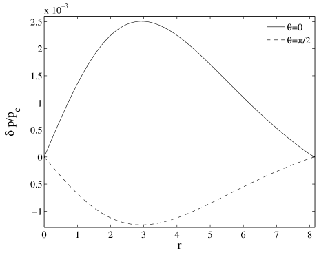
Figure 1: Profile of the relative pressure perturbation $\delta p/p_{c}$ [computed on the $z$-axis ($\theta=0$) and on the $xy$-plane ($\theta=\pi/2$)] obtained from Eqs. (56-57) with $n=0$ and $\lambda=\lambda 0$.

In the following, we use the same setup, Eq. (57), to provide initial data in both the linear and nonlinear codes. Correspondingly, the computation of $\delta p$ is needed to get a handle on the magnitude of the deviation from sphericity. The best indicator is given by the ratio $\delta p/p_{c}$, where $p_{c}$ is the central pressure of the star. Fig. 1 displays the profile of $\delta p/p_{c}$, at the pole and at the equator, as a function of the Schwarzschild radial coordinate $r$ for $\lambda=\lambda 0=0.001$. For simplicity, we consider only $n=0$ perturbations, with four values for the amplitude, namely $\lambda=[0.001,~{}0.01,~{}0.05,~{}0.1]$, in order to see, in the 3D code, how the transition from linear to nonlinear regime occurs. Maxima and minima of the initial pressure perturbation for the different values of the initial perturbation amplitude $\lambda$ can be found in Table 2.

III.2 Metric-perturbation setup: the 1D linear code

Let us turn now to discuss the implementation of Eq. (57) in the two codes and the corresponding treatment of the related initial metric perturbation. As discussed in Refs. Gundlach and Martin-Garcia (2000); Seidel (1990), the even-parity metric perturbation of a general (nonstatic) spherically symmetric space-time is described by 3 degrees of freedom ($k_{{\ell}m},\chi_{{\ell}m}$ and $\psi_{{\ell}m}$) that are the solution of three coupled partial differential equations. On the static TOV background, only $k_{{\ell}m}$ and $\chi_{{\ell}m}$ are independent degrees of freedom of the gravitational field, and their evolution equations are decoupled from that of $\psi_{{\ell}m}$, which can be obtained at every time-step once $\chi_{{\ell}m}$ and $k_{{\ell m}}$ are known. The recovery of $\psi_{{\ell m}}$ from $\chi_{{\ell m}}$ and $k_{{\ell m}}$, that is needed in the 3D case, will be explicitly discussed in Sec. III.3 below. By contrast, for the 1D implementation one only needs to specify initial data for $\chi_{{\ell}m}$, $k_{{\ell}m}$, and their time derivatives. This is accomplished by solving the constraints under a number of assumptions related to the physics that we want to investigate. First of all, we consider only axisymmetric perturbations ($m=0$) and we restrict ourselves to the dominant quadrupole mode (${\ell}=2$). Then, since in this work we are not interested in $w$-mode excitation, we impose the conformally flat condition ($\chi_{20}=0$) (see Refs. Nagar et al. (2004); Bernuzzi and Nagar (2008a) for details). With These hypotheses, we solve the Hamiltonian constraint, namely Eq.(7) of Ref. Bernuzzi and Nagar (2008a), for $k_{20}$. This is done on a grid $r\in[0,r_{\rm max}]$, with $r_{\rm max}\gg R$ and with boundary condition $k_{20}=0$ at $r=0$ and at $r=r_{\rm max}$. We impose $\dot{k}_{20}=\dot{\chi}_{20}=0$ for simplicity, but we are aware that this is inconsistent with the condition that $H_{20}\neq 0$ initially and thus the momentum constraints should also be solved. However, since the effect is a small initial transient in the waveforms that quickly washes out before the quasiharmonic oscillation triggered by the perturbation $H_{20}$ sets in, we have decided to maintain the initial-data setup simple. Figure 2 synthesizes the information about the initial data. The top panel shows (as a solid line) the profile of $k_{20}$ (versus Schwarzschild radius) corresponding to the perturbation $\lambda=\lambda 0$ of Table 2; the bottom panel shows (as a solid line) the initial profile of the Zerilli-Moncrief function $\Psi^{(\rm e)}_{20}$ outside the star.

III.3 Metric-perturbation setup: the 3D nonlinear code

In the 3D code we setup the same kind of initial condition as in the 1D code, but the procedure is more complicated as one needs to reconstruct the full 3D metric on the Cartesian grid. In addition, the main difference with respect to the 1D case is that the perturbative constraints are expressed using a radial isotropic coordinate $\bar{r}$ instead of the Schwarzschild-like radial coordinate $r$. This is done because $\bar{r}$ is naturally connected to the Cartesian coordinates in which the code is expressed, i.e. $\bar{r}=\sqrt{x^{2}+y^{2}+z^{2}}$. The initialization of the metric in the 3D case has to follow four main steps: (i) The perturbative constraints are solved, (ii) The multipolar metric components are added to the unperturbed background TOV metric; (iii) The resulting metric is written in Cartesian coordinates; (iv) It is interpolated on the Cartesian grid.

Let us then recall some useful formulas. At the background level, the TOV metric in isotropic coordinates reads

$$ds^{2}_{0}=-e^{2a}dt^{2}+e^{2b}\left(d{\bar{r}}^{2}+{\bar{r}}^{2}d\Omega^{2}\right)\ ,$$ (58)

where $d\Omega=d\theta^{2}+\sin^{2}d\phi^{2}$. The relations between the Schwarzschild and isotropic radial coordinates in the exterior are given by

$$r ={\bar{r}}\left(1+\frac{M}{2{\bar{r}}}\right)^{2}\ ,$$ (59)

$${\bar{r}} =\frac{1}{2}\left(\sqrt{r^{2}-2Mr}+r-M\right)\ ,$$ (60)

and in the interior by

$$r ={\bar{r}}e^{2b(r)}\ ,$$ (61)

$${\bar{r}} =Cr\exp{\left[\int^{r}_{0}dx\frac{1-\sqrt{1-2m(x)/x}}{x\sqrt{1-2m(x)/x}}\right]}\ ,$$ (62)

where

$$C =\frac{1}{2R}\left(\sqrt{R^{2}-2MR}+R-M\right)$$

$$\times\exp{\left[-\int_{0}^{R}dx\frac{1-\sqrt{1-2m(x)/x}}{x\sqrt{1-2m(x)/x}}\right]}.$$ (63)

In terms of the isotropic radius, the perturbative Hamiltonian constraint explicitly reads

$$k^{{\ell m}}_{,{\bar{r}}{\bar{r}}}+\dfrac{k^{{\ell m}}_{,{\bar{r}}}}{{\bar{r}}}\left[1+\left(1-\dfrac{2m(r)}{r}\right)^{1/2}\right]$$

$$+e^{2b}\left(8\pi e-\dfrac{\Lambda}{r^{2}}\right)k^{{\ell m}}-\dfrac{1}{{\bar{r}}}\left(1-\dfrac{2m(r)}{r}\right)^{1/2}\!\!\!\chi_{,{\bar{r}}}^{{\ell m}}$$

$$-e^{2b}\left(\dfrac{\Lambda+2}{2r^{2}}-8\pi e\right)\chi^{{\ell m}}=-\dfrac{8\pi(p+e)H^{{\ell m}}}{C_{s}^{2}}\,,$$ (64)

where $r\equiv r({\bar{r}})$ according to Eq. (59) and (61).

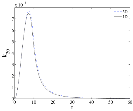
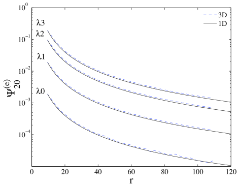
Figure 2: (color online) Initial-data setup in the 1D and 3D codes. Top panel: Profiles of the $k_{20}$ multipole at $t=0$ versus the Schwarzschild radial coordinate r, obtained from the solution of the perturbative Hamiltonian constraint with $\lambda=\lambda 0$ and $n=0$. Bottom panel: Profiles of $\Psi^{(\rm e)}_{20}$ at $t=0$ versus the Schwarzschild radial coordinate $r$, for different values of the initial perturbation $\lambda$. Both panels compare the results of the computations of the 1D and 3D codes.

After solving the TOV equations, we choose a profile for $H_{{\ell m}}$, impose the conformal-flatness condition $\chi_{\ell m}=0$, and solve Eq. (III.3) for $k_{{\ell m}}$. As we discussed in the previous section, one also needs to impose on $\psi_{\ell m}$ some condition that can be regarded as an initial gauge condition. Then $(\chi_{{\ell m}},k_{{\ell m}},\psi_{{\ell m}})$ must be inserted in the explicit expression of the (even-parity) metric perturbation

$$\delta s^{2}_{\ell m} =\big{\{}(\chi_{\ell m}+k_{\ell m})e^{2a}dt^{2}-2\psi_{\ell m}e^{a+b}dtd\bar{r}$$

$$+e^{2b}\left[(\chi_{\ell m}+k_{\ell m})d{\bar{r}}^{2}+{\bar{r}}^{2}k_{\ell m}d\Omega\right]\big{\}}Y_{{\ell}m}\ .$$ (65)

In the absence of azimuthal and tangential velocity perturbations, in Schwarzschild coordinates and in the Regge-Wheeler gauge, from the momentum-constraint equation, namely Eq. (95) of Ref. Gundlach and Martin-Garcia (2000), one obtains

$$\psi_{{\ell m},r}=-\dfrac{2\left[m(r)+4\pi r^{3}p(r)\right]}{r-2m(r)}\psi\,,$$ (66)

which, once solved, gives

$$\psi_{\ell m}(r)=\tilde{C}\exp\left[-\int_{0}^{r}dx\dfrac{2\left(m(x)+4\pi x^{3}p(x)\right)}{x-2m(x)}\right].$$ (67)

The requirement $\psi_{\ell m}\to 0$ for large $r$, like for $k_{\ell m}$, implies $\tilde{C}=0$; therefore, the metric perturbation is given by Eq. (III.3) with $\psi_{\ell m}=\chi_{\ell m}=0$. The full metric in isotropic coordinates is obtained as $ds^{2}=ds_{0}^{2}+\delta s_{{\ell m}}^{2}$. This metric is transformed to Cartesian coordinates and then it is linearly interpolated onto the Cartesian grid used to solve the coupled Einstein-matter equations numerically. To ensure a correct implementation of the boundary conditions (i.e. $k_{{\ell m}}\to 0$ when $\bar{r}\to\infty$), the isotropic radial grid used to solve Eq. (III.3) is much larger ($\bar{r}\sim 3000$) than the corresponding Cartesian grid ($\bar{r}\sim 208$) and the spacing is much smaller.

One proceeds similarly for the matter perturbation: From a given profile for $H_{\ell m}(r)$, the pressure perturbation $\delta p(r,\theta)$ is computed and from this the total pressure is given by $p+\delta p$. This is interpolated on the Cartesian grid to finally obtain the vector of the conserved hydrodynamics variables $(D,S^{i},\tau)$.

The consistency of the initial-data setup procedure in both the PerBACCo 1D linear code and in the Cactus-Carpet-CCATIE-Whisky 3D nonlinear code is highlighted in Fig. 2. The top panel of the figure compares the profiles of $k_{20}$ in the 1D case (solid line) and in the 3D case (dashed line) for $\lambda=\lambda 0$ and $n=0$. The small differences are related to a slightly different location of the star surface in the two setups and to the different resolution of the grids. The bottom panel of Figure 2 contrasts the Zerilli-Moncrief functions $\Psi^{(\rm e)}_{20}$ from the 1D code (solid lines) with those extracted (at $t=0$) from the numerical 3D metric (dashed lines). For all initial conditions, the curves show good consistency.

IV Results

The presentation of our results is organized in the following way. In Sec. IV.1 we focus first on radial oscillations, that are always present due to numerical discretization error. Then we concentrate on nonradial stellar oscillations and we compare the 1D and 3D metric waveforms (Sec. IV.2) and curvature waveforms (Sec. IV.3). In Sec. IV.4 we discuss advantages and disadvantages of these two wave-extraction techniques. Finally, we discuss the use of quadrupole-type formulas in Sec. IV.5, while Sec. IV.6 is devoted to the analysis of nonlinear couplings between oscillation modes.

IV.1 Radial oscillations

The unperturbed configuration A0 has been stably evolved for about 20 ms. The numerical 3D grid used for this simulation is composed of two concentric cubic boxes with limits $[-32,\,32]$ and $[-16,\,16]$ in all the three Cartesian directions. The boxes have resolutions $\Delta_{xyz}=0.5$ and $0.25$ respectively; bitant symmetry, i.e. the $z<0$ domain is copied from the $z>0$ domain instead of being evolved, was imposed as a boundary condition in order to save computational time.

The truncation errors of the numerical scheme trigger (physical) radial oscillations of (mainly) the fundamental mode $F$ and the first overtones. We have checked that these frequencies agree with those computed evolving the radial pulsation equation with the perturbative code. This comparison is shown in Table 3. We note in passing that our numbers are in perfect agreement with those of Table I of Ref. Font et al. (2002).

Table 3: Frequencies of the fundamental radial mode of model A0.

n	Pert.[Hz]	3D [Hz]	Diff. [%]
0	1462	1466	0.3
1	3938	3935	0.1
2	5928	5978	0.8

As a further check, the entire sequence of uniformly rotating models with mass $M=1.4$ and nonrotating limit A0 has been evolved. Simulations were done with a cubic grid with limits $[-32,\,32]$ in each direction, and uniformly spaced with grid spacing $\Delta_{xyz}=0.5$. As before, we have imposed bitant symmetry. The sequence of initial models has been computed by means of the version of the RNS code Stergioulas and Friedman (1995) implemented in Whisky. For the equilibrium properties of the models, see Ref. Dimmelmeier et al. (2006).

The fluid modes of this sequence were previously investigated in different works, using various approaches Font et al. (2001); Stergioulas et al. (2004); Dimmelmeier et al. (2006). With our general-relativistic 3D simulations we are able to study the effect of rotation on the radial mode and compare the results with those obtained via approximated approaches. Our results are summarized in Table 4. We have found that the frequencies computed by Dimmelmeier et al. Dimmelmeier et al. (2006) in the conformally flat approximation are consistent with ours (the difference is of the order of few percents); on the other hand, the results of Stergioulas et al. Stergioulas et al. (2004), obtained in the Cowling approximation, differ of about a factor two, consistently with the estimates of Ref. Yoshida and Kojima (1997). In all cases, the frequencies decrease if the rotation increases and the trend is linear in the rotational parameter $\beta\equiv T/|W|$, the ratio between the kinetic rotational energy and the gravitational potential energy.

Table 4: Frequencies of the fundamental radial mode of models in the sequence AU of uniformly rotating polytropic stars of Refs. Stergioulas et al. (2004) and Dimmelmeier et al. (2006). The frequency of model AU0 (A0) has also been computed in Ref. Font et al. (2002) ($1450$ Hz) and in this work ($1462$ Hz), where a finer grid was used (see Table 3). The data in the column marked as “CF” refer to Table III of Ref. Dimmelmeier et al. (2006). The data in the column marked as “Cowling” refer to Table II of Ref. Stergioulas et al. (2004).

MODEL	F [Hz]	F(CF) [Hz]	F(Cowling) [Hz]
AU0	1444	1458	2706
AU1	1369	1398	2526
AU2	1329	1345	2403
AU3	1265	1283	2277
AU4	1166	1196	2141
AU5	1093	1107	1960

IV.2 Nonradial oscillations: comparing 1D and 3D metric waveforms

Let us now turn to the discussion of nonspherical oscillations and to the related extraction of waveforms from 1D and 3D simulations. We consider a star perturbed with an ${\ell}=2$, $H_{{\ell}0}(r)$ profile with $n=0$, according to the procedure outlined in Sec. III. This system is evolved separately with the two codes and the related gravitational waveforms are compared.

We focus first on the discussion of the outcome of the 1D linear code. We accurately performed very long simulations, whose final time is about $1$ s. The extraction radii for the Zerilli-Moncrief function extend as far as $\bar{r}=420$ ($\simeq 300M$). The resolution of the radial grid is $\Delta r=0.032$, which corresponds to having 300 points inside the star. Fig. 3 shows the Zerilli-Moncrief function $\Psi^{(\rm e)}_{20}$ (for $\lambda=\lambda 1$) extracted at different radii. It is plotted versus the observer retarded time, namely $u=t-r_{*}$, where $r_{*}$ is the Regge-Wheeler tortoise coordinate $r_{*}=r+2M\log[r/(2M)-1]$ and $M$ is the mass of the star.

The farther observers that are shown in Fig. 3 are sufficiently deep in the wave-zone that the initial offset, that is typically present due to the initial profile of $k_{20}$, is small enough to be considered negligible. We checked the convergence of the waves with the extraction radius using as a reference point the maximum of $\Psi^{(\rm e)}_{20}$. This point can be accurately fitted, as a function of the extraction radius, with

$$\max{\left(\Psi^{(\rm e)}_{20}\right)}\sim a^{\infty}+\frac{a^{1}}{r}\,.$$ (68)

The extrapolated quantity $a^{\infty}$ allows an estimate of the error related to the extraction at finite distance

$$\delta a\equiv\frac{\Big{|}a^{\infty}-\max{\left(\Psi^{(\rm e)}_{20}(r)\right)}\Big{|}}{a^{\infty}}\,.$$ (69)

The values of $\delta a$ for different radii are $\delta a\simeq 0.5$ for $r=25M$, $\delta a\simeq 0.09$ for $r=50M$, $\delta a\simeq 0.017$ for $r=100M$ and $\delta a<0.016$ for $r>200M$.

The waveform can be described by two different phases: (i) an initial transient, of about half a gravitational-wave cycle, say up to $u\simeq 50$, related to the setup of the initial data, followed by (ii) a quasiharmonic oscillatory phase, where the matter dynamics are described in terms of the stellar quasinormal modes. From the Fourier spectrum of $\Psi^{(\rm e)}_{20}$ over a time interval from $1$ to about $30$ ms (namely $u\in[50,\,6000]$), we found that the signal is dominated by the $f$ mode (at frequency $\nu_{f}=1581$ Hz) with a much lower contribution of the first $p$ mode (at frequency around $\nu_{p_{1}}=3724$ Hz). The frequency of the $f$ mode agrees with that of Ref. Font et al. (2002) within $1-2$%. The accuracy of our linear code for frequencies obtained from Fourier analysis on such long time series has been checked in Refs. Nagar and Diaz (2004); Bernuzzi and Nagar (2008a) and is better than 1% on average. We mention that the Fourier analysis of the matter variable $H_{\ell m}$ permits to capture some higher overtones than the $p_{1}$ mode, although they are essentially not visible in the gravitational-wave spectrum. In a first approximation, the waveform can thus be thought as the superposition of damped harmonic oscillators

$$\Psi_{20}\sim\sum_{k=0}^{N}A_{2k}\cos(2\pi\nu_{2k}u+\phi_{2k})\exp(-\alpha_{2k}u)\ ,$$ (70)

and we aim at determining the quantities $A_{2k}$, $\phi_{2k}$, $\nu_{2k}$ and $\alpha_{2k}$ from a standard nonlinear least-square fit. Since the frequency $\nu$ is also independently known from the Fourier analysis, it is used as feedback for the fit. In addition, to quantify the global differences between the “actual” and the “fitted” time series, we compute the ($l^{2}$) scalar product

$$\Theta(X,Y)=\frac{\sum_{j}X_{j}Y_{j}}{\sqrt{\sum_{j}\left(X_{j}\right)^{2}}\sqrt{\sum_{j}\left(Y_{j}\right)^{2}}}\ ,$$ (71)

which is bounded in the interval $[0,\,1]$, and then we look at the residual ${\cal R}=1-\Theta$. This residual gives us a relative measure of the reliability of the fit. In addition we use the $l^{\infty}$ distance:

$${\cal D}(X,Y)=\max_{j}{\left|X_{j}-Y_{j}\right|}\,,$$ (72)

that gives the maximum difference between the two time series. We will use the quantities ${\cal R}$ and ${\cal D}$ also as measures of the global agreement between the 3D and 1D waveforms.

Table 5: Perturbative 1D evolution with $\lambda=\lambda 1$: results of the fit to a superposition of two fluid modes [see Eq. (70)] over the interval $u\in[0,200000]$, i.e. about 1 s (cf.Fig. 4). For this fit, ${\cal R}\simeq 1.6\times 10^{-6}$ and ${\cal D}\simeq 3.6\times 10^{-5}$ (see text for explanations).

[arbitrary units]	$\nu$ [Hz]	$\alpha$ [$\rm s^{-1}]$
$A_{20}$=$1.3145_{-2}^{+2}\times 10^{-3}$	$\nu_{20}$=$1583.7369_{-1}^{+2}$	$\alpha_{20}$=$3.7358_{-9}^{+9}$
$A_{21}$=$3.517_{-12}^{+13}\times 10^{-5}$	$\nu_{21}$=$3706.9413_{-11}^{+11}$	$\alpha_{21}$=$0.421_{-6}^{+8}$

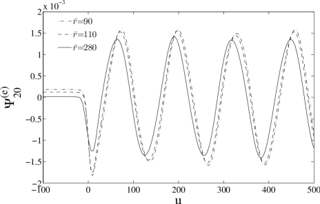
Figure 3: Evolution of the Zerilli-Moncrief function, extracted at various isotropic radii $\bar{r}$, versus the retarded time $u$, for the 1D linear code evolution with $\lambda=\lambda 1$. Note how the initial offset decreases with the extraction radius.

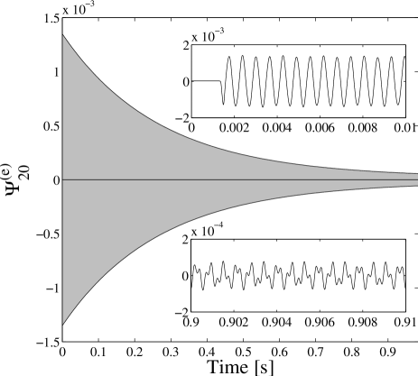
Figure 4: Evolution of the Zerilli-Moncrief function, extracted at isotropic radius $\bar{r}=280$ for the same evolution of Fig. 3 versus the retarded time $u$ expressed now in seconds (1 dimensionless time unit is equal to $4.92549\times 10^{-6}$ s). The main panel shows only the envelope of the waveform that is dominated by the damping time of the $f$ mode ($\tau_{f}\simeq 0.27$ s). The two insets represent the full waveform at early (top) and late (bottom) times. The presence of the overtone is evident in the oscillations at late times.

On the interval $u\in[50,6000]$, the waves can be perfectly (${\cal R}\simeq 7\times 10^{-4}$, ${\cal D}\simeq 6\times 10^{-6}$) represented by a one-mode expansion, $N=1$, as the waveform is dominated by $f$-mode oscillations. The frequency we obtain, $\nu_{20}=1580.79\pm 0.01$ Hz, is perfectly consistent with that obtained via Fourier analysis; for the damping time, we estimate $\alpha_{20}=3.984\pm 0.066$ $\rm s^{-1}$ and thus $\tau_{20}=\alpha_{20}^{-1}\simeq 0.25$ s. If we consider the entire duration (1s) of the signal (see the inset in Fig. 4), it is clear that a one-mode expansion is not sufficient to accurately reproduce the waveform. The Fourier analysis of the waveform in two different time intervals, one for $t\lesssim 0.5$ s and one for $t\gtrsim 0.5$, reveals that in the second part of the signal the $p_{1}$ mode, which has longer damping time, clearly emerges and must be taken into account. We fit the entire signal with two modes, namely $N=2$, with a global agreement of ${\cal R}\simeq 2\times 10^{-6}$ and ${\cal D}\simeq 4\times 10^{-5}$. The results of the fit are reported in Table 5. The frequencies are slightly larger than those computed via Fourier analysis and via the fit procedure restricted to only one mode on a shorter interval. They are, however, still consistent. The damping times are $\tau_{20}=0.268$ s and $\tau_{21}=2.37$ s, with errors of the order of $0.1$% and $2$% respectively.

At this stage, we have clearly assessed the accuracy of the waveforms computed via our 1D code; in the following we shall consider these waveforms (extracted at the farthest observer) as exact for all practical purposes. We turn now to the discussion of the metric waveforms extracted from the 3D code and we compare them to the exact, perturbative results for different values of the perturbation $\lambda$.

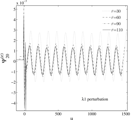
Figure 5: Zerilli-Moncrief normalized metric waveforms shown versus the observer retarded time $u=t-r_{*}$ at different extraction radii ($\bar{r}=30$ to $\bar{r}=110$), for a 3D evolution with perturbation $\lambda=\lambda 1$. The initial part of the waveform is dominated by a pulse of junk radiation.

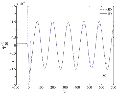
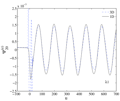
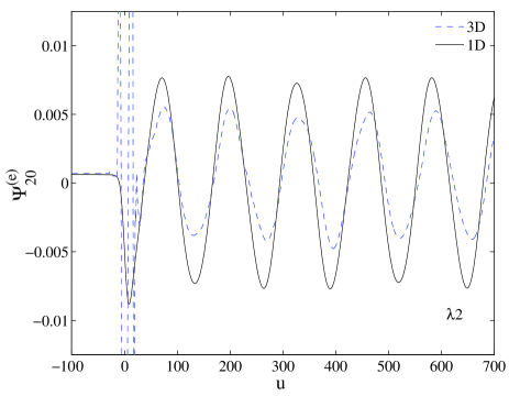
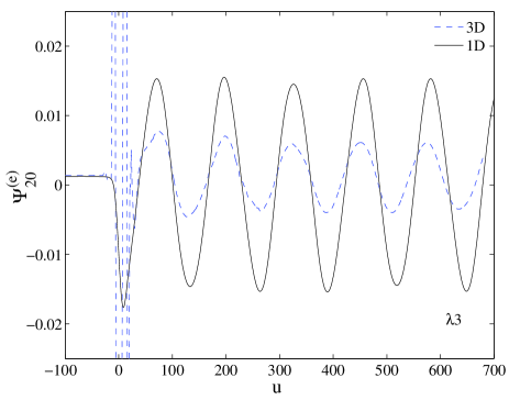
Figure 6: (color online) Metric waveforms extracted at $\bar{r}=110$ computed from 3D simulations (dashed lines) and 1D linear simulations (solid lines) for different values of the perturbation $\lambda$. If $\lambda$ is sufficiently small (e.g. , $\lambda\lesssim 0.01$) the outcomes of the two codes show good agreement. If the “perturbation” is large ($\lambda\sim 0.1$), nonlinear effects become dominating.

The 3D simulations are performed over grids with three refinement levels and cubic boxes with limits $[-120,\,120]$, $[-24,\,24]$ and $[-12,\,12]$ in each direction. The resolutions of each box are $\Delta_{xyz}=0.5$, $0.25$ and $0.125$, respectively. Equations are evolved only on the first octant of the grid and symmetry conditions are applied. The outermost detector is located at isotropic-coordinate radius $\bar{r}=110$ ($\sim 80M$).

Figure 5 is obtained with perturbation $\lambda=\lambda 1$. It displays the Zerilli-Moncrief normalized metric waveforms, extracted on coordinate spheres of radii $\bar{r}\in\{30,~{}60,~{}90,~{}110\}$ and plotted versus the (approximate) retarded time $u=t-r_{*}$, where $r_{*}=r+2M\log[r/(2M)-1]$. Here, $r$ is the areal radius of the spheres of coordinate radius $\bar{r}$ and $M$ is the Schwarzschild mass enclosed in $\bar{r}$ Abrahams and Price (1996); Allen et al. (1998c); Pazos et al. (2007). This figure is the 3D analogous of Fig. 3. The 1D and 3D waveforms look qualitatively very similar apart from the presence of a highly-damped, high-frequency oscillation at early times. In Sec. IV.4 we will argue that this oscillation is essentially unphysical because its amplitude grows linearly with the extraction radius $\bar{r}$, instead of approaching an approximately constant value (as it happens instead for the subsequent fluid-mode oscillations). Section IV.4 is devoted to a thorough discussion of these issues; for the moment, we simply ignore this problem and focus our attention only on the part of the waveform dominated by fluid modes.

Each panel of Fig. 6 compares the 1D, exact $\Psi^{(\rm e)}_{20}$ (dashed lines) with that computed via the 3D code (solid lines) for the four values of the perturbation $\lambda$. The extraction radius is (in both codes) $\bar{r}=110$ and this implies that a nonzero, constant offset for $u\lesssim 0$ is present. Note, in this respect, the good consistency between 3D and 1D results for $u\lesssim 0$, confirming here the information enclosed in the bottom panel of Fig. 2. After the initial high-frequency (unphysical) oscillations, the top-left panel of Fig. 6 shows that an excellent agreement between the waveforms is found when the perturbation is small. Then, for larger values of $\lambda$ (until it assumes values that cannot be considered a perturbation anymore) the amplitude of the oscillation in the 3D simulations becomes smaller with respect to the linear case, suggesting that nonlinear couplings (specifically, couplings with overtones as well as couplings with the radial modes) are redistributing the energy of the ${\ell}=2$, $m=0$ oscillations triggered by the initial perturbation. In Sec. IV.6, we will argue that couplings between modes become more and more relevant when the perturbation increases, giving a quantitative explanation to the phenomenology that we observe. This effect is summarized in Fig. 7, which displays the amplitude $A_{20}$ obtained by fitting the waveform with the template Eq. (70) versus the magnitude of the perturbation for 1D (linear) and 3D (nonlinear) simulations. It is evident from the figure that there is a consistent deviation from linearity already when the perturbation is relatively small ($\lambda\lesssim 0.02$). As a measure of the global agreement between 1D and 3D waveforms (as a function of the initial perturbation $\lambda$) we list in Table 6 the $l^{2}$ residuals ${\cal R}=1-\Theta(\Psi^{\rm 1D},\Psi^{\rm 3D})$ and the $l^{\infty}$ distances ${\cal D}(\Psi^{\rm 1D},\Psi^{\rm 3D})$.

Table 6: “Global-agreement” measures computed on the interval $\Delta u=[50,3000]$ (after the junk burst) at the outermost detector. Here, ${\cal R}=1-\Theta(\Psi^{\rm 1D},\Psi^{\rm 3D})$ is the $l^{2}$ residual while ${\cal D}(\Psi^{\rm 1D},\Psi^{\rm 3D})$ is the $l^{\infty}$ distance.

$\lambda$	$\mathcal{R}$	$\mathcal{D}$
$\lambda 0$	$3.07\times 10^{-2}$	$7.93\times 10^{-5}$
$\lambda 1$	$4.88\times 10^{-2}$	$7.79\times 10^{-4}$
$\lambda 2$	$1.63\times 10^{-1}$	$2.78\times 10^{-3}$
$\lambda 3$	$9.96\times 10^{-1}$	$2.04\times 10^{-2}$

Table 7: Frequency analysis of the 3D waveforms (see Fig. 6) over the interval $u\in[50,\,3000]$. The frequencies from 1D simulations are $\nu_{f}^{\rm 1D}=1581$ Hz and $\nu_{p_{1}}^{\rm 1D}=3724$ Hz. From left to right the columns report the amplitude of the perturbation, the $f$-mode frequency, its relative difference with the 1D value, the $p_{1}$-mode frequency and its relative difference with the 1D value.

$\lambda$	$\nu_{f}^{\rm 3D}$ [Hz]	Diff.[%]	$\nu_{p_{1}}^{\rm 3D}$ [Hz]	Diff.[%]
$\lambda 0$	1578	0.2	3705	0.5
$\lambda 1$	1576	0.3	3705	0.5
$\lambda 2$	1573	0.5	3635	2.4
$\lambda 3$	1623	2.7	3565	4.3

The 3D waveforms for $\lambda 0$ and $\lambda 1$ turn out to be damped on a time scale of about 20 ms. This damping time is much shorter than the one of the $f$ mode or $p_{1}$ mode, as computed via the 1D approach. This effective-viscosity damping time $\tau^{\rm visc}$ (that is related to the inverse of the viscosity coefficient) can be extracted by means of the fit analysis discussed above for the waveform. We have found that $\tau^{\rm visc}$ depends on the initial perturbation, being $\tau^{\rm visc}\simeq 0.022,0.132,0.203,0.129$ s respectively for $\lambda=\lambda 0,\lambda 1,\lambda 2,\lambda 3$. The best agreement with the expected physical value of $\tau_{20}=0.268$ s is obtained for $\lambda=\lambda 2$; both for larger and smaller perturbations the 3D results show even shorter damping times. The errors on these quantities are of the order of $0.5$%. The interpretation of these results may include two different effects. The smaller damping time of the wave for the $\lambda=\lambda 3$ perturbation with respect to the $\lambda=\lambda 2$ one may be interpreted as due to the nonlinear couplings that allow the disexcitation of the fundamental mode in other channels; as it can be seen from Fig. 7 and Fig. 19, the importance of nonlinear effects is larger for the simulation with perturbation $\lambda=\lambda 3$. However, for perturbations smaller than $\lambda=\lambda 2$ the effective viscosity is not found to decrease towards the expected perturbative value, as it could have been expected from the above argument. This discrepancy might be due to the numerical viscosity proper of the evolution scheme. Such numerical viscosity would have a bigger influence in low-perturbation simulations, where the energy lost from the fundamental mode into other modes is smaller (while in higher-perturbation simulations the coupling of modes is the dominant effect). Although the detailed analysis of the numerical viscosity of the 3D code is beyond the scope of the present work, we checked that, as expected, it depends on the grid resolution. We performed tests using a three-refinement-level setup with the resolution of the coarsest grid (with limits $[-120,120]$ in the three directions) set at the values $\Delta_{xyz}=2$ (low), $1$ (medium) and $0.5$ (high). Using these three resolutions, we observed that, in the case of the coarsest grid, there was an initial explosion in the amplitude, then followed by a strong damping during the first five gravitational-wave cycles. This shows that this resolution is not even sufficient to extract the qualitative behavior of the waveform. On the other hand, the other two resolutions did not show any qualitative difference in addition to the different value of the “effective viscosity”, that is smaller for higher resolutions. We also checked whether there is a measurable effect due to the artificial atmosphere. Focusing only on the $\lambda=\lambda 0$ perturbation, we varied the value of the rest-mass density of the atmosphere in the range $\rho_{\rm atm}=10^{[-5,-6,-7]}\rho_{\rm max}$, without finding any significant influence on the values of $\tau^{\rm visc}$. We leave to forthcoming studies a detailed analysis of the viscosity of the 3D evolution code.

Finally, we have also Fourier-transformed the 3D waveforms to extract the fluid-mode frequencies and we have compared them with the linear ones. This comparison is shown in Table 7. Apparently, the frequency of the $f$ mode (that dominates the signal) is less sensitive to nonlinear effects than its amplitude, as it can be seen from the fact that only the $\lambda=\lambda 3$ initial data are such to force the star to oscillate at a frequency slightly different from that of the linear approximation. On the other hand, the first overtone (the $p_{1}$ mode) seems more sensitive. It is in any case remarkable that for $\lambda=\lambda 0$ and $\lambda=\lambda 1$ the frequencies from 3D and 1D simulations coincide at better than 1%, suggesting that the main gravitational-wave frequencies are only mildly affected by nonlinearities.

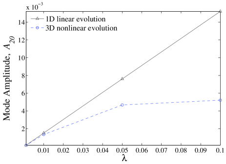
Figure 7: (color online) Comparison between the oscillation amplitude $A_{20}$ (from fits) in the 1D (linear) and 3D (nonlinear) simulations versus the initial perturbation $\lambda$. Deviations from linearity are occurring already for very small values of $\lambda$.

IV.3 Nonradial oscillations: comparing 1D and 3D curvature waveforms

This section is devoted to the comparison between 1D and 3D curvature waveforms. In the 1D code one can use the relation

$$r\psi_{4}^{{\ell m}}=r\ddot{h}^{\ell m}=N_{\ell}\left(\ddot{\Psi}_{{\ell m}}^{(\rm e)}+{\rm i}\ddot{\Psi}_{{\ell m}}^{(\rm o)}\right)$$ (73)

to obtain the Newman-Penrose scalar (multiplied by the extraction radius) $r\psi_{4}^{\ell m}$ from the gauge-invariant metric master functions. Because of our choice of initial conditions, we shall consider only $\Psi^{(\rm e)}_{20}$ in the following.  The second time-derivative of $\Psi^{(\rm e)}_{20}$ is computed via finite differencing, by applying twice a first-order derivative operator with 4th-order accuracy. By contrast, in the 3D code $\psi_{4}^{20}$ is extracted independently of the metric waveform. Then, one computes $r\psi_{4}^{20}$, where $r$ is an approximated radius from Eq. (59) with $M=1.4$.

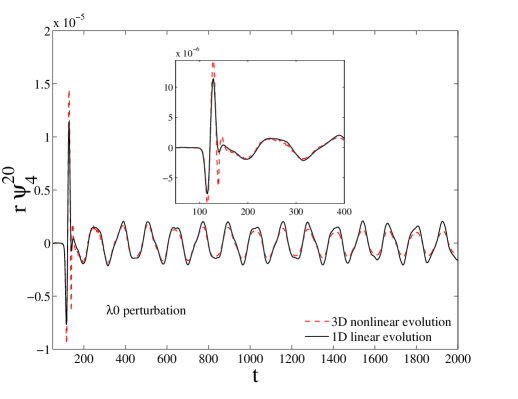
Figure 8: (color online) 1D versus 3D evolution of the $r\psi_{4}^{20}$ curvature waveform for perturbation $\lambda=\lambda 0$. The initial transient is consistent between the two evolutions. The inset concentrates on the initial part of the waveform.

Figure 8 displays the $r\psi_{4}^{20}$ waveforms from 1D (solid line) and 3D (dashed line) evolutions with perturbation $\lambda=\lambda 0$. The extraction radius is $\bar{r}=110$ in both codes. Visual inspection of the figure immediately suggests that: (i) The initial transient in the 1D metric waveform preceding the setting in of the quasiharmonic $f$-mode oscillation results in a highly damped, high-frequency oscillation; (ii) The initial transient radiation has the same qualitative shape in both the 1D and 3D waveforms, although the amplitude of the oscillation is larger in the latter case. At this point one should note that: (i) In the 1D case, although the conformally flat condition is imposed at $t=0$, the constraint is solved numerically and thus a small violation of this condition occurs; (ii) The violation is expected to be larger in the 3D case, because of the larger truncation errors. It is in any case remarkable that, as the figure shows, these errors (e.g. the slightly different shapes of $k_{20}$, the linear interpolation from spherical to Cartesian coordinates, etc.) are sufficiently under control to produce the same qualitative behavior besides small quantitative differences in the initial part of the 1D and 3D waveforms.

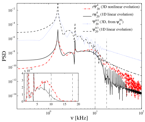
Figure 9: (color online) Comparison of the PSD of various waveforms. The PSD of the $r\psi_{4}^{20}$ and $\Psi^{(\rm e)}_{20}$ from the 1D code are compared with those from the 3D code, obtained after integration. The initial perturbation is $\lambda=\lambda 0$. The $w$-mode frequencies $w_{1}$ and $w_{2}$ are superposed to the spectra as vertical dot-dashed lines. See text for discussions.

The question that occurs at this point is whether the violation of the conformally flat condition introduces some amount of physical $w$-mode excitation in the waveforms. To answer this question we show in Fig. 9 the Fourier power spectral density (PSD) of the $r\psi_{4}^{20}$ waveforms of Fig. 8. The PSD is computed all over the waveform and not only during the “ring-down”, because of the difficulty of separating reliably this part from the “precursor” Bernuzzi et al. (2008). We are aware of the problems related to the precise determination the $w$-mode frequencies and to their location in the waveform (see Refs. Bernuzzi et al. (2008); Nollert (1999) for a related discussion), and in particular of the fact that the Fourier analysis can not provide accurate and definitive answers, essentially because, in the presence of damped signals with frequencies comparable to the inverse of the damping time, the Fourier spectrum results in a broad peak. However it represents a fundamental part of the analysis and, in the present case, is preferable to a fitting procedure because of the already mentioned problem of separating the precursor from the ring-down part.

The dashed-dotted vertical lines of Fig. 9 locate the first two $w$-mode frequencies of this model, $\nu_{w_{1}}=10.09$ kHz and $\nu_{w_{2}}=17.84$ kHz. These frequencies have been computed by K. Kokkotas and N. Stergioulas via an independent frequency-domain code and have been kindly given to us for this specific comparison. Two of the maxima of the PSD of the 3D $r\psi_{4}^{20}$ waveform can be associated to the frequencies $\nu_{w_{1}}$ and $\nu_{w_{2}}$, even if they are in a region very close to the noise. The frequency $\nu_{w_{1}}$ is probably slightly excited also in the 1D case (see inset), while only noise is present around $\nu_{w_{2}}$. In Fig. 9 we show also the PSD of the 1D $\Psi^{(\rm e)}_{20}$ (dashed dark line) and the one of the 3D $\Psi^{(\rm e)}_{20}$ (dashed light line) obtained from the double time-integration of $\psi_{4}^{20}$. In both cases, it is not possible to disentangle $\nu_{w_{1}}$ and $\nu_{w_{2}}$ from the background noise.

The fact that a signal characterized by highly damped modes is much less evident in the PSD of the metric waveform than in the corresponding curvature one is simply due to the second derivative that relates the two gauge-invariant functions. When space-time modes are excited, the metric waveform is (approximately) composed by a pure ring-down part plus a tail contribution Price (1972), that is $\Psi^{(\rm e)}_{20}\approx e^{-\sigma t}+\beta t^{-7}$, where $\sigma=\alpha+i\omega$ ($\alpha$ is the inverse of the damping time and $\omega$ the $w$-mode frequency) and $\beta$ is a numerical coefficient. When one takes two time derivatives to compute $r\psi_{4}^{20}$ from $\Psi^{(\rm e)}_{20}$, the tail contribution is suppressed by a factor $t^{-2}$ and the oscillatory part of the waveform emerges more sharply. This comparison suggests that the best way to extract information about $w$ modes (especially when their contribution is small) is, in general, to look at $r\psi_{4}^{\ell m}$. In addition, it also highlights that, while it is not possible to exclude the presence of $w$ modes in the $r\psi_{4}^{\ell m}$ signal due to the small violation of the conformally flat condition at $t=0$, at the same time we can not definitely demonstrate that those high frequencies present near the noise are attributable to $w$ modes. In the next section we are going to show similar analyses on the spectra computed from $\Psi^{(\rm e)}_{20}$ waveforms extracted á la Abrahams-Price from the 3D simulation.

Finally, the global-agreement measures on the $\psi_{4}$ extraction are $\mathcal{R}\simeq 1.42\times 10^{-2}$ and $\mathcal{D}\simeq 9.09\times 10^{-7}$, and they highlight some differences between the linear and the nonlinear approach.

The analysis discussed so far indicates that, in the present framework, the wave-extraction procedure based on the Newman-Penrose scalar $\psi_{4}$ seems to produce waveforms that, especially at early times, are more accurate than the corresponding ones extracted via the Abrahams-Price metric-perturbation approach. However, one of the big advantages of the latter method is that the waveforms $h_{+}$ and $h_{\times}$ are directly available at the end of the computation, and thus ready to be injected in some gravitational-wave–data-analysis procedure. By contrast, if we prefer to use Newman-Penrose wave-extraction procedures (which are the most common tools employed in numerical-relativity simulations nowadays), we must consistently give prescriptions to obtain $\Psi^{(\rm e/o)}_{{\ell m}}$ from $\psi_{4}^{\ell m}$. To do so, one needs to perform a double (numerical) time integration, with at least two free integration constants to be determined to correctly represent the physics of the system. Inverting Eq. (73) following the considerations of Sec. II.3.1, we obtain the following result [see Eq. (38)]:

$$rh^{\ell m} =N_{\ell}\left(\Psi^{({\rm e})}_{{\ell m}}+{\rm i}\Psi^{({\rm o})}_{{\ell m}}\right)$$ (74)

$$=\int_{0}^{t}dt^{\prime}\int_{0}^{t^{\prime}}dt^{\prime\prime}r\psi^{4}_{\ell m}(t^{\prime\prime})+Q_{0}+Q_{1}t+Q_{2}t^{2},$$

$$=r\tilde{h}_{\ell m}(t)+Q_{0}+Q_{1}t+Q_{2}t^{2},$$

where $Q_{0}$, $Q_{1}$ and $Q_{2}$ are (still) undetermined integration constants, which are complex if $m\neq 0$. Note that this relation does not involve the $Q_{2}$ integration constant only if finite-radius extraction effects can be considered negligible (see below).

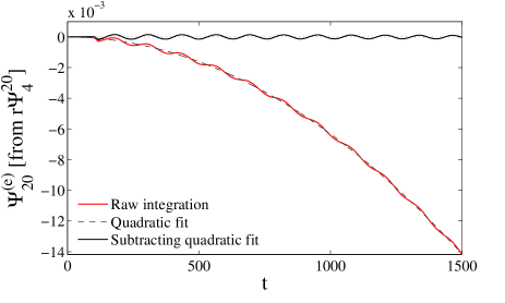
Figure 10: (color online) Recovery of $\Psi^{(\rm e)}_{20}$ from two successive time integrations of $r\psi_{4}^{20}$ extracted from the 3D simulation with initial perturbation $\lambda=\lambda 0$. After the subtraction of a quadratic floor the waveform correctly oscillates around zero.

Our aim is to recover the metric waveform that corresponds to the 3D $r\psi_{4}^{20}$ waveform that we have characterized above. We consider the waveform of Fig. 8 up to $t=1500$, where the reduction in amplitude due to numerical viscosity is already of the order of $30\%$ with respect to the exact linear waveform. This sampled curvature waveform is integrated twice in time, from $t=0$ without fixing any integration constant to obtain $r\tilde{h}_{\ell m}(t)$.

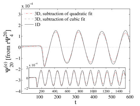
Figure 11: (color online) Selecting the best fitting function for the 3D integrated-and-subtracted metric waveform. The dash-dotted line refers to the curve obtained with the subtraction of a cubic fit and the dashed line to the curve obtained with the subtraction of a quadratic fit. They are very similar to each other and to the 1D waveform (solid line). Contrary to the case of the extracted metric waveform, no initial burst of radiation is present in the 3D integrated-and-subtracted waveform.

The raw result of this double integration is shown in Fig. 10. The “average” of the oscillation does not lay on a straight line, as it does instead in the case of the waveforms of binary black-hole coalescence discussed in Ref. Damour et al. (2008), but rather it shows also a quadratic correction due to the finite extraction radius (see discussion in Sec. II.3.1).

Indeed, when a “floor” of the form $P(t)=Q_{0}+Q_{1}t+Q_{2}t^{2}$ is subtracted, the resulting metric waveform is found to oscillate around zero, as it can be seen in Fig. 10 and Fig. 11, which focuses on the beginning of the oscillation. The values of the coefficients of $P(t)$ obtained from the fit are $Q_{0}=-4.338\times 10^{-7}$, $Q_{1}=-1.2462\times 10^{-7}$ and $Q_{2}=-6.2046\times 10^{-9}$. The fact that $Q_{0}<0$ is connected to the choice of initial data we made (i.e. $k_{20}\neq 0$ at $t=0$). Then, $Q_{1}\neq 0$ indicates that the system is (slightly) out of equilibrium already at $t=0$ and it is thus emitting gravitational waves since $\dot{\Psi}^{(\rm e)}_{20}(0)\neq 0$. This is consistent with the choice of initial data we made, that is a perturbation that appears instantaneously at $t=0$ without any radiative field obtained from the solution of the momentum constraint (since we use time-symmetric initial perturbations, for which $\dot{k}_{20}=\dot{\chi}_{20}=0$).

We tested the robustness of the quadratic fit by adding a cubic term $Q_{3}t^{3}$ to $P(t)$ and then fitting again. In Fig. 11, we compare the 3D $\Psi^{(\rm e)}_{20}$ waveform corrected with a cubic fit (dashed line) with the one corrected with a quadratic fit (dash-dotted line) and with the “exact” 1D metric waveform (solid line) output by the PerBACCo code. Note that the 1D waveform has been suitably timeshifted in order to be visually in phase with the others at the beginning of the simulation. The figure suggests that the effect of the cubic correction is almost negligible (one only finds slight changes in the very early part of the waveform). The values of the fitting coefficients $Q_{i}$ are $Q_{0}=-1.0096\times 10^{-5}$, $Q_{1}=-6.3331\times 10^{-9}$, $Q_{2}=-4.747\times 10^{-8}$, $Q_{3}=6.7114\times 10^{-14}$. The fact that $Q_{3}$ is many orders of magnitude smaller than the other coefficients is a good indication that the quadratic behavior is indeed the best choice here. Consistently with the curvature waveform of Fig. 8, we note the excellent agreement between 1D and 3D (integrated) metric waveforms also in the initial part of the waveform, i.e. up to $t\simeq 200$ (corresponding to the high-frequency oscillation in $r\psi_{4}^{20}$). Evidently, this is in contrast with the Abrahams-Price metric waveform in the top-left panel of Fig. 6 (we will elaborate more on this in the next section).

Finally, we point out that the coefficient $Q_{2}(r)$ shows, as expected, a clear trend towards zero for increasing values of the extraction radius.

IV.4 Advantages and disadvantages of the Abrahams-Price metric wave-extraction procedure

The analysis carried out so far suggests that both the Regge-Wheeler-Zerilli metric-based and the Newman-Penrose $\psi_{4}$-curvature-based wave-extraction techniques can be employed to extract reliable gravitational waveforms from simulations of compact self-gravitating systems. For the particular case of an oscillating neutron star as considered here, both extraction methods allow to obtain waveforms that are in very good agreement with the linear results. Despite this success, the two approaches are not free from drawbacks. Let us first focus on $r\psi_{4}^{\ell m}$ curvature waveforms. The comparison between 1D and 3D $r\psi_{4}^{20}$ waveforms in Fig. 8 (as well as between integrated metric waveforms in Fig. 11) shows good consistency between the two (as long as the effects of numerical viscosity on the evolution of the system remain negligible). As we mentioned above, we think that the most important information enclosed in Fig. 8 is that the differences between the high-frequency oscillations in the initial part of the waveforms (where $w$ modes are probably present in the 3D case) are small. This fact makes us confident that the violation of the 3D Hamiltonian constraint at $t=0$ (due to its approximate solution) as well as the violation of the conformally flat condition are sufficiently small to avoid pathological behavior during evolution. A further confirmation of the accuracy of the evolution and of the curvature extraction is given by Fig. 12: The quantities $r\psi_{4}^{20}$ extracted at various radii ($\bar{r}\in\{30,60,90,110\}$) and plotted versus retarded time are all superposed. This confirms the theoretical expectations of the peeling theorem Stewart (1991) and indicates (once more) that the quantity $r\psi_{4}^{20}$ is accurately computed. In Fig. 12, $r$ is obtained from $\bar{r}$ via Eq. (59). The retarded time is approximated with the standard $r_{*}$, where the constant mass $M=1.4$ has been used. In our setup, the only subtle issue about $r\psi_{4}^{{\ell m}}$ seems to be the computation of the corresponding metric waveform via a double time integration. Although we were able to obtain a rather accurate metric waveform, the time-integration procedure (including the evaluation of the integration constants) may not be likewise straightforward in other physical settings.

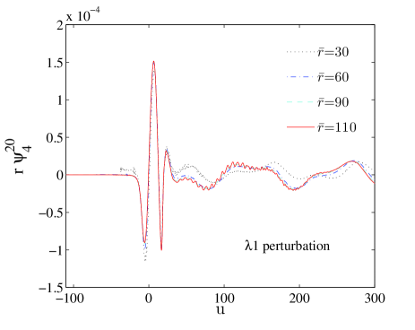
Figure 12: (color online) The quantities $r\psi_{4}^{20}$ extracted at different radii are superposable (as expected from the “peeling” theorem). See text for further explanation.

By contrast, the Abrahams-Price wave-extraction procedure directly produces the metric waveform and no time integrations are needed. For this reason, it looks a priori more appealing than $\psi_{4}$ extraction. Unfortunately, the results that we have presented so far (notably our Fig. 6) indicate that this computation can be very delicate and can give unphysical results even in a very simple system like an oscillating polytropic star: we have found that $\Psi^{(\rm e)}_{20}$ extracted in this way is unreliable at early times, because of the presence of high-frequency, highly damped oscillations, that are instead absent in both the 1D linear metric waveforms and the 3D metric waveforms time-integrated from $r\psi_{4}^{20}$. The unphysicalness of this initial “burst” of radiation is evident from Fig. 13, where the extractions at various radii $\bar{r}\in\{30,60,90,110\}$ of the quantity $\Psi^{(\rm e)}_{20}$ are compared: the amplitude grows with $\bar{r}$, instead of decreasing progressively to approach a constant value (as it is the case for the $f$-mode–dominated subsequent part of the waveform).

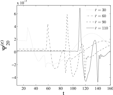
Figure 13: Metric waveforms computed via the Abrahams-Price procedure and extracted at different radii, for a 3D evolution with perturbation $\lambda=\lambda 0$. Note how the amplitude of the initial burst grows linearly with $\bar{r}$.

The weird behavior at early times of the extracted $\Psi^{(\rm e)}_{20}$ indicates that this function does not satisfy the Zerilli equation in vacuum. Consistently, the perturbative Hamiltonian constraint in vacuum, Eq. (III.3) with $H_{20}=0$, constructed from the 3D metric multipoles $(\chi_{20},k_{20})$, must be violated of some amount in correspondence of the junk . This reasoning suggests that the junk may be the macroscopic manifestation of the inaccuracy in the initial-data setup at $t=0$ (i.e. of solving the linearized Hamiltonian constraint first and then interpolating), possibly further amplified by the wave-extraction procedure. This statement in itself looks confusing, because we have learned, from the analysis of $\psi_{4}$, that the Einstein (and matter) equations are accurately solved and that the errors made around $t=0$ due to the violation of Hamiltonian constraint are relatively negligible. The relevant question is then: is it possible that small numerical errors, almost negligible in $r\psi_{4}^{20}$, may be amplified in $\Psi^{(\rm e)}_{20}$ at such a big level to produce totally nonsensical results? The following discussion proposes some heuristic explanation.

To clarify the setup of our reasoning, let us first remind the reader of the basic elements of the Abrahams-Price metric wave-extraction procedure and, in particular, the role of Eq. (II.1). At a certain evolution time $t$, the numerical metric $g_{\mu\nu}(t)$ is known at a certain finite accuracy on the Cartesian grid. One selects coordinate extraction spheres of coordinate radius $\bar{r}=\sqrt{x^{2}+y^{2}+z^{2}}$ on which the metric is interpolated via a second-order Lagrangian interpolation. Isotropic-coordinate systems $(\bar{r},\theta,\phi)$ naturally live on these spheres and thus one defines spherical harmonics. Then, the metric $g_{\mu\nu}$ is formally decomposed in a Schwarzschild “background” $g^{0}_{\mu\nu}$ plus a perturbation $h_{\mu\nu}$. The next step is to choose a coordinate system in which the background metric is expressed. The standard approach is to use Schwarzschild coordinates, although this choice actually introduces systematic errors that may relevantly affect the waveforms. This has been recently demonstrated in Ref. Pazos et al. (2007). Although we are aware of this fact, we prefer to neglect this source of error, on which we will further comment below. Choosing Schwarzschild coordinates means that one needs to compute a Schwarzschild radius $r$. This is given by the areal radius of the extraction two-spheres. Proceeding further, $h_{\mu\nu}$ is decomposed into seven (gauge-dependent) even-parity $(H_{0},H_{1},H_{2},h_{0}^{(\rm e)},h_{1}^{(\rm e)},G,K)$ and three (gauge-dependent) odd-parity multipoles (that we do not consider here). From combinations of the seven even-parity multipoles and of their radial derivatives, see Eqs. (41) and (42) of Ref. Nagar and Rezzolla (2005), one obtains the gauge-invariant functions $k_{{\ell m}}$ and $\chi_{{\ell m}}$, as well as the derivative $\partial_{r}k_{{\ell m}}$. The last step is the computation of the Zerilli-Moncrief function via Eq. (II.1). Various sources of errors are present. In particular, we mention the errors originating from: (i) the discretization of $g_{\mu\nu}$ (and its derivatives), from the numerical solution of Einstein’s equations; (ii) the interpolation from the Cartesian grid to the isotropic grid; (iii) the computation of the metric multipoles via numerical integration over coordinate (gauge-dependent) two-spheres. Our aim is to investigate how these inaccuracies on $(\chi_{{\ell m}},k_{{\ell m}},\partial_{r}k_{{\ell m}})$ can show up in $\Psi^{(\rm e)}_{{\ell m}}$ at large extraction radii. In the limit $r\gg M$, Eq. (II.1) reads

$$\Psi^{(\rm e)}_{{\ell m}}=\dfrac{2r}{\Lambda(\Lambda-2)}\left(\chi_{{\ell m}}-r\partial_{r}k_{{\ell m}}+\dfrac{\Lambda}{2}k_{{\ell m}}\right),$$ (75)

that is

$$\Psi^{(\rm e)}_{{\ell m}}\propto rZ_{{\ell m}}\,,$$ (76)

where $Z_{{\ell m}}=\chi_{{\ell m}}-r\partial_{r}k_{{\ell m}}+\Lambda/2k_{{\ell m}}$ and $r$ is the areal radius of the coordinate two-spheres. The Abrahams-Price wave-extraction procedure introduces then errors both on $r$ and $Z_{{\ell m}}$. In particular, the errors on the (gauge-invariant) multipoles $(\chi_{{\ell m}},k_{{\ell m}},\partial_{r}k_{{\ell m}})$ conspire in a global error on $Z_{{\ell m}}$. In a numerical simulation one has $Z_{{\ell m}}=Z_{{\ell m}}^{\rm Exact}+\delta Z_{{\ell m}}$ and $r=r^{\rm Schw}+\delta r$. Here $Z_{{\ell m}}^{\rm Exact}$ is computed from $(\chi_{{\ell m}}^{\rm Exact},k_{{\ell m}}^{\rm Exact})$, that are solutions of the perturbation equation on a Schwarzschild background, and $r^{\rm Schw}$ is the radial Schwarzschild coordinates; $\delta Z_{{\ell m}}$ encompasses all possible errors due to the multipolar decomposition procedure, and $\delta r$ various inaccuracies related to the determination of the areal radius (e.g. , those related to gauge effects). As a result, for the “extracted” Zerilli-Moncrief function we can write

$$\Psi^{(\rm e)}_{{\ell m}}\approx\Psi^{\rm Exact}_{{\ell m}}+r^{\rm Schw}\delta Z_{{\ell m}}+\delta rZ_{{\ell m}}^{\rm Exact}.$$ (77)

This equation shows that, if $\delta Z_{{\ell m}}$ is not zero at a certain time (and does not decrease in time like $1/r^{\rm Schw}$) there is a contribution to the global error on $\Psi^{(\rm e)}_{{\ell m}}$ that grows linearly with the extraction radius. This qualitative picture is consistent with what we observe in the 3D waveforms: a small error on $\delta Z_{20}$ introduced at $t=0$, because of the approximate solution of the constraints (as indicated by the analysis of $r\psi^{20}_{4}$ curvature waveforms), can show up as a burst of radiation whose amplitude increases linearly with the observer location. Note that what really counts here is the error budget at the level of $(\chi_{20},k_{20},\partial_{r}k_{20})$ and the related violation of the perturbative Hamiltonian constraint, Eq. (III.3). Indeed, it might occur that, even if the 3-metric $\gamma_{ij}$ is very accurate and the constraints are well satisfied at this level, the extraction procedures adds other errors (for example due to the multipolar decomposition, computation of derivatives etc.) that may be eventually dominating in $\delta Z_{20}$. This observation may partially justify why $r\psi_{4}^{20}$ is well behaved, while $\Psi^{(\rm e)}_{20}$ is not. Finally, we note that in our evolution $\delta r$ is typically very small, so that we have $r^{\rm Schw}\approx r$ with good accuracy.

Because of the complexity of the 3D wave-extraction algorithm, we were able neither to push forward our level of understanding, nor to precisely diagnose the cause of the aforementioned errors . This is now beyond the scope of the present work and will deserve more attention in the future. By contrast, we can exploit the simpler computational framework offered by the 1D PerBACCo code to “tune” the error $\delta Z_{{\ell m}}$ in order to produce some initial “spurious” burst of radiation, and then possibly observe that its amplitude grows linearly with $\bar{r}$. In the 1D code $\delta r$ is zero by construction, so that all errors are concentrated on $\delta Z_{{\ell m}}$. The constrained scheme adopted in the perturbative code (which is second-order convergent) allows to accurately compute the multipoles $(\chi_{{\ell m}},k_{{\ell m}})$ at every time step, and the Hamiltonian constraint is satisfied by construction. Then, $\partial_{r}k_{{\ell m}}$ is obtained via direct numerical differentiation of $k_{{\ell m}}$. Consequently, the error $\delta Z_{lm}$ depends on the resolution $\Delta r$ as well as on the order of the finite-differencing representation of $\partial_{r}k_{{\ell m}}$.

In the following we shall analyze separately the effect of resolution and of the approximation scheme adopted for the numerical derivatives. First, we approximate $\partial_{r}k_{{\ell m}}$ with its standard first-order finite-differencing representation, i.e. $\partial_{r}k_{{\ell m}}\approx(k_{j+1}^{{\ell m}}-k_{j}^{{\ell m}})/\Delta r$ and we study the behavior of the extracted $\Psi^{(\rm e)}_{{\ell m}}$, computed using Eq. (II.1), versus extraction radius and resolution. Second, we use a fixed $\Delta r$, but we vary the accuracy of the finite-differencing representation of $\partial_{r}k_{{\ell m}}$, contrasting first-order, second-order and fourth-order stencils. The results of these two analyses, for ${\ell}=2$, $m=0$, are shown in Figs. 14 and 15 respectively.

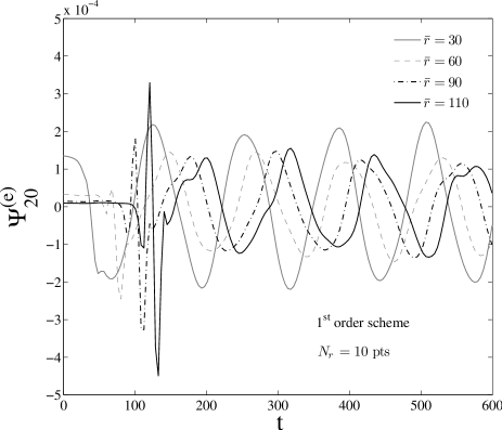
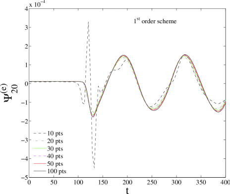
Figure 14: (color online) Metric waveforms from linear 1D evolutions. Top panel: Low resolution simulation. A burst of junk radiation at early times is present and its amplitude grows linearly with the extraction radius. Bottom panel: By increasing the resolution, the initial junk disappears.

In the top panel of Fig. 14 $\partial_{r}k_{20}$ is approximated at first-order, with a resolution of 10 points inside the star ($\Delta r\sim 0.9$). This resolution approximately corresponds to the resolution of the coarsest refinement level used in the 3D code. The extracted waveform $\Psi^{(\rm e)}_{20}$ is shown at different observers, $\bar{r}\in\{30,60,90,110\}$: An initial burst of junk radiation develops at early times and its amplitude grows linearly with the extraction radius (and it keeps growing for $\bar{r}>110$). This behavior looks identical to that found in the 3D simulations. In the bottom panel of Fig. 14 we focus on $\bar{r}=110$ only, but vary the number of radial points $N_{r}$ inside the star, namely $N_{r}\in\{10,20,30,40,50,100\}$. The figure shows that the initial junk is not present at higher resolutions ($N_{r}\geq 20$) and that the waveform converges to the exact profile. But varying the resolution only shifts the occurrence of the burst at farther radii: observers at $\bar{r}\gg 110$ still see this burst appear and grow linearly with $\bar{r}$.

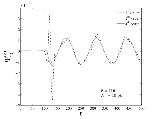
Figure 15: The amount of junk radiation present in the waveforms extracted in the 1D code is smaller when higher-order differential operators are used in Eq. (II.1) to compute the the Zerilli-Moncrief function.

A complementary analysis is shown in Fig. 15, where we fix the resolution at $N_{r}=10$ (for $\bar{r}=110$), but we change the accuracy of the numerical derivative $\partial_{r}k_{20}$. As expected, the initial junk disappears when the accuracy of the numerical differential operator is increased: a second-order operator produces only a small amplitude bump, that is not present when the fourth-order operator is employed. At this stage, the conclusion is clear: the convergence of the Zerilli-Moncrief function computed from the separate knowledge of the multipoles $k_{{\ell m}}$ and $\chi_{{\ell m}}$ is a delicate issue that must be analyzed with care according to the physical problem under consideration. The violation of the perturbative Hamiltonian constraint and, in particular, the accuracy of the numerical derivative $\partial_{r}k_{{\ell m}}$ (note that we refer to the induced violation at the level of the wave extraction and not at that of the solution of the perturbation equations) seems to play an important role in the convergence properties of the waveforms. The main conclusions of the aforementioned numerical tests are: (i) The errors in $\Psi^{(\rm e)}_{20}$ seem to behave like suggested in Eq. (77); (ii) The phenomenon occurs in the same way in both the 1D and 3D code, although the fine details of the oscillation are different.

Focusing on the 1D PerBACCo code, an accurate $\Psi^{(\rm e)}_{{\ell m}}$ is obtained using sufficiently high resolution ($N_{r}=300$) as well as a fourth-order representation for $\partial_{r}k_{{\ell m}}$. These prescriptions are accurate enough for the problem addressed in this work, although they may not be sufficient for other stellar models or other initial perturbations. For example, using the PerBACCo code, with the same initial data setup discussed here, in order to study the time evolution of perturbations of stars with realistic EOS proved that higher resolutions are typically needed to produce convergent waveforms of comparable accuracy Bernuzzi and Nagar (2008a). Likewise, for a polytropic EOS and initial data given by a Gaussian pulse in $\Psi^{(\rm e)}_{20}$, the same Ref. Bernuzzi and Nagar (2008a) showed that at least fourth-order accuracy in $\partial_{r}k_{20}$ is needed in order to have a consistent extraction of $\Psi^{({\rm e})}_{20}$ already at $t=0$ (see Appendix A of Ref. Bernuzzi and Nagar (2008a)). This suggests that the presence of linearly growing junk radiation in the computation of $\Psi^{(\rm e)}_{{\ell m}}$ from the multipoles $(k_{{\ell m}},\chi_{{\ell m}})$ can appear ubiquitously in the time evolutions of the perturbation equations with the PerBACCo code. The presence of this junk in $\Psi^{(\rm e)}_{{\ell m}}$ is the macroscopic manifestation of the violation of the perturbative Hamiltonian constraint due to errors (notably, in the discretization of the derivatives) introduced in the wave-extraction procedure. These (typically small) numerical errors are eventually magnified by the presence of an overall $r$ factor in Eq. (75). Note that this phenomenon occurs even if the computation of the multipoles $(k_{{\ell m}},\chi_{{\ell m}})$ is very accurate and the Hamiltonian constraint is satisfied by construction in the evolution algorithm. The analysis that we have presented here suggests that either increasing the resolution or, more reasonably, implementing higher-order differential operators in the perturbative “extraction” procedure are viable proposals to compute convergent waveforms.

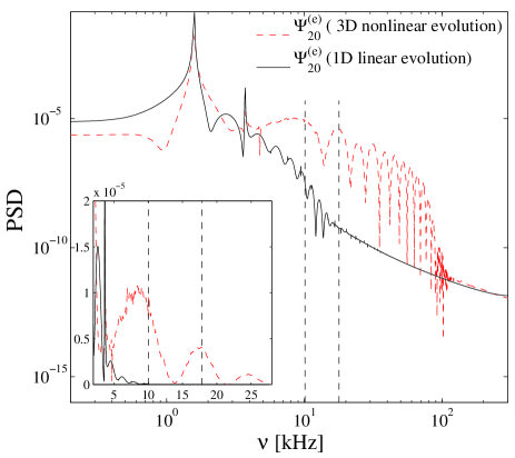
Figure 16: (color online) PSD of the 3D metric waveforms (dashed line) extracted á la Abrahams-Price (at $\bar{r}=110$) and the corresponding 1D waveform (solid line) for a simulation with perturbation $\lambda=\lambda 0$. The Fourier spectrum of the junk radiation is compatible with some $w$-mode frequencies.

In the 3D case the situation is more involved and we have not succeeded in making statements as solid as in the 1D case. We can only rely on analogies: (i) The appearance of the junk occurs in a way similar to the 1D case when the accuracy of the 1D Zerilli function is low; (ii) The two time evolutions look qualitatively very similar. Yet, it is not technically possible to use in the 3D code resolutions equivalent to those of the 1D code. By analogy with our perturbative results, we can only conclude that it is not unreasonable that the junk in the 3D waveforms is the macroscopic manifestation of inaccuracies hidden in the implementation of the Abrahams-Price wave-extraction procedure. The analysis presented here points out that such metric wave-extraction procedures require typically more subtle care than expected and these subtleties must be kept in mind in developing more modern wave-extraction routines.

The PSD of $\Psi^{(\rm e)}_{20}$ in both the 1D case (solid line) and 3D case (dashed line) is displayed in Fig. 16. The perturbation is $\lambda=\lambda 0$ and the extraction radius is $\bar{r}=110$. The spectrum of the 3D Zerilli waveform is consistent with what we observed in $r\psi_{4}^{20}$ below $10$ kHz, but it looks different at higher frequencies (compare it with that of the “integrated” $\Psi^{(\rm e)}_{20}$ in Fig. 9): here the PSD shows broad peaks attributable to the initial part of the waveform. Recovering the reasoning started in the previous section about the presence of the $w$ modes, we can observe that the frequencies contained in the junk are compatible with the $w$-mode frequencies $\nu_{w_{1}}$ and $\nu_{w_{2}}$ (indicated by dashed vertical lines in Fig. 16). However, since such frequencies belong to an unphysical part of the waveform, we prefer to consider them unphysical as well.

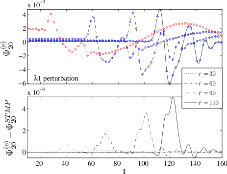
Figure 17: (color online) The top panel compares the standard Zerilli-Moncrief $\Psi^{(\rm e)}_{20}$ (depicted with lines) and the generalized $\Psi^{\rm STMP}_{20}$ (depicted with point markers) for the first part of the gravitational-wave signal in a simulation with perturbation $\lambda=\lambda 1$. The waves extracted at four radii $\bar{r}\in\{30,60,90,110\}$ are shown. The bottom panel shows that the present junk radiation negligibly depends on the choice of the coordinates of the background metric.

We conclude by mentioning, in passing, that the initial junk radiation is essentially not related to the systematic error introduced by fixing Schwarzschild coordinates for the background metric $g^{0}_{\mu\nu}$. This fact is suggested by Fig. 17, where we contrast the standard Zerilli-Moncrief function $\Psi^{(\rm e)}_{20}$ (which assumes Schwarzschild coordinates for the background) with the generalized $\Psi^{\rm STMP}_{20}$ one based on the Sarbach-Tiglio Sarbach and Tiglio (2001) and Martel-Poisson Martel and Poisson (2005) perturbation formalism, which does not require any gauge-fixing condition for the background submanifold $M^{2}$. This particular simulation was performed over a grid with three refinement levels and cubic boxes with limits [-120, 120], [-24,24] and [-12,12]. The resolution of each box is coarser than in the previous simulations, namely $\Delta_{xyz}=1.875$, $0.9375$ and $0.46875$ respectively. Evidently, with this resolution the waveforms are less accurate, but we do not mind at this stage, since we are interested in an intrinsic comparison between extraction procedures at fixed resolution. The function $\Psi^{\rm STMP}_{{\ell m}}$ that we use is given by the straightforward implementation of Eq. (4.23) of Ref. Martel and Poisson (2005). Note that this expression is equivalent to the combination of Eqs. (20), (25), (26) and (27) of Ref. Sarbach and Tiglio (2001). The top panel of Fig 17 displays $\Psi^{(\rm e)}_{20}$ (lines) and $\Psi^{\rm STMP}_{20}$ (point markers) for observers at $\bar{r}\in\{30,60,90,110\}$. It highlights that the differences in the early-time part of the waveforms are very small. By contrast, the bottom panel of the figure, showing the difference $\Psi^{(\rm e)}_{20}-\Psi^{\rm STMP}_{20}$, indicates that removing (part of) the systematic errors generates some improvement, but this is too small to be of any relevance. This analysis suggests that the inaccuracies in the early-time part of the waveform are essentially not related to the specific computation of the (generalized) Zerilli function, but rather connected to the underlying multipolar extraction infrastructure (grid setup, approximate solution of the constraints, interpolation procedures, computation of the derivatives of the metric etc.), on which we have relatively little control. A comprehensive analysis of the problems related to the generalized extraction procedure will be presented elsewhere Bernuzzi and Nagar (2008b). We remark, however, that systematic effects that are very small in our physical system, as emphasized by our Fig. 17, may be not small in other situations, as found in Ref. Pazos et al. (2007). For this reason, we emphasize that the formalism of Refs. Sarbach and Tiglio (2001); Martel and Poisson (2005) is the actual correct metric formalism to extract waveforms out of a numerical space-time that can be considered a small deformation of the Schwarzschild one. As such, it must be taken into account properly in numerical codes.

IV.5 Generalized quadrupole-type formulas

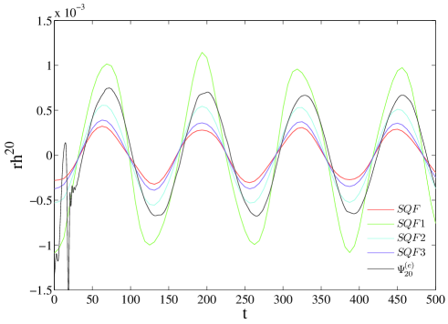
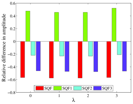
Figure 18: (color online) Comparison between different wave-extraction procedures in the 3D simulations, in particular between the SQFs and the gauge-invariant wave-extraction procedure. The left panel shows the waveforms. The frequencies almost coincide, while the amplitudes are strongly underestimated in all cases except SQF1, where the amplitude is strongly overestimated. The right panel shows the relative difference between the amplitudes of the various SQFs and the Abrahams-Price wave extraction. These amplitudes are estimated with the fit procedures.

Finally, we study the performances of the various generalized quadrupole-type formulas that we have introduced in Sec. II.3. The results of our analysis are shown in Fig. 18. The left panel of the figure displays $rh^{20}$ waveforms obtained via the SQF1, SQF2, SQF3 and SQF4 [see Eqs. (52–55)] for perturbation $\lambda=\lambda 0$. The right panel complements this information by showing (for several perturbation magnitudes $\lambda$) the relative difference in amplitude between the various SQFs and the corresponding gauge-invariant Zerilli-Moncrief function $\Psi^{(\rm e)}_{20}$. This analysis highlights that the quadrupole formula gives an excellent approximation to the phasing of the actual signals. By contrast, there is a systematic over- or under-estimation of the amplitude depending on the choice of SQF.

A related observation is that the discrepancy between the quadrupole formula and the gauge-invariant waveform is not due to the fact that waveforms are extracted at a finite radius. Our results are consistent with those of Shibata and Sekiguchi Shibata and Sekiguchi (2003), who performed an analysis similar to ours (and also considered uniformly rotating stars), but without the possibility of contrasting their results with linear evolutions. In this respect, the main conclusion of Ref. Shibata and Sekiguchi (2003) was that, although the amplitude of the waveform is systematically underestimated by the quadrupole formula (47), it is however sufficiently accurate to capture both the frequency and the phasing (that are the most important quantities for detection) of the waveforms in a proper way. These results are fully confirmed here using totally different codes.

IV.6 Nonlinearities

In this section we comment on the onset of nonlinear effects for high values of the initial perturbation amplitude $\lambda$, showing, for the first time using full GR simulations, evidences for mode couplings and for the appearance of nonlinear harmonics.

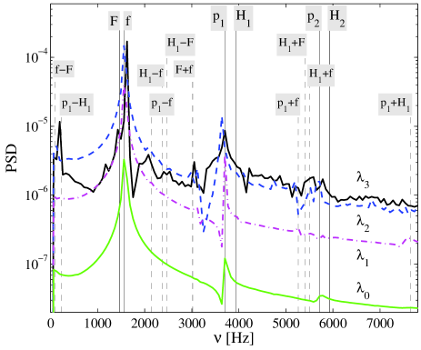
Figure 19: (color online) PSD of the quantity $\langle\rho\rangle_{20}(t)$ [see Eq. 78] for different values of the initial perturbation amplitude $\lambda$. The spectra of the (${\ell}=2$, $m=0$) mode obtained in simulations with larger perturbations contain more frequencies, which originate from the nonlinear couplings with the overtones and with the radial modes.

In the linear regime ($\lambda=\lambda 0$) the star is oscillating at, essentially, the frequency of the fundamental quadrupolar proper fluid (quasinormal) mode of pulsation. The principal linear modes excited are thus the $({\ell},m)=(2,0)$ one and its overtones. For growing values of the initial perturbation, we observe that in 3D simulations, differently from the linear ones, the amplitude of the multipole $\Psi^{(\rm e)}_{20}$ does not increase proportionally to $\lambda$ but, instead, is progressively reduced (see Fig. 7). This fact could be interpreted as the results of a typical phenomenon in nonlinear systems in which linear modes couple, generating nonlinear harmonics. Naively, one could think that the “energy” associated to the ${\ell}=2$ mode is redistributed to the others while the system departs from the linear regime. As we saw in Sec. IV.1, radial modes of oscillation are already present in the evolution of the equilibrium models. As a consequence, we expect to reveal couplings between nonradial and radial modes ($F$ and its overtones $H_{1},H_{2},...$) as a result of the onset of some nonlinear effect. In addition, we detect signals in multipoles of $\Psi^{(\rm e)}_{\ell m}$ with $\ell=4,6$ and $m=0,4$, that are even-parity axisymmetric modes and nonaxisymmetric modes triggered by the Cartesian grid. The amplitudes are very weak compared to those of the $f$ mode for any value of $\lambda$, typically 2 orders of magnitude smaller for ${\ell}=4,m=0$ and 3 orders of magnitude for the others, but in principle they are present and must be considered. As far as the odd-parity modes with $m=1,2,3$, and ${\ell}=3,5$ are concerned, they are all forbidden by the symmetry imposed on the computational domain (octant).

As a strategy to study nonlinearities, we consider the rest-mass–density projections:

$$\langle\rho\rangle_{{\ell m}}(t)\equiv\int d^{3}x\rho(t,\mathbf{x})Y^{*}_{{\ell m}}$$ (78)

and we apply to them the Fourier analysis. Like all the global variables, $\rho$ contains all the frequencies of the system. Its projections in Eq. (78) allow to separate the contribution of each mode $({\ell},m)$. Fig. 19 shows the power spectrum of $\langle\rho\rangle_{20}$ for the four different values of $\lambda$. The signal for $\lambda=\lambda 0$ contains the 3 frequencies of the linear modes $f$, $p_{1}$ and $p_{2}$. The same happens for $\lambda=\lambda 1$ and $\lambda=\lambda 2$: the amplitudes of the linear modes grow linearly with $\lambda$ and some new frequencies are present with small power for $\lambda=\lambda 2$. In the case of $\lambda=\lambda 3$, which corresponds to a pressure perturbation of 10% of the central TOV value, the spectra is rich of nonlinear harmonics. Most of them can be recognized as due to weak couplings, i.e. sums and differences of linear mode frequencies $\nu_{1}\pm\nu_{2}$, also called combination tones. In particular we identify the nonlinear harmonics of the $f$ mode and its overtone $f\pm p_{1}$ and many frequencies $f\pm F$, $f\pm H_{1}$ and $p_{1}\pm H_{1}$ due to the radial and nonradial mode couplings. Such couplings have been previously and extensively studied in Refs. Font et al. (2001); Stergioulas et al. (2004); Dimmelmeier et al. (2006) using the Cowling approximation as well as the conformally flat approximation to GR. In addition, the couplings between radial and nonradial modes have been studied in detail in Ref. Passamonti et al. (2007) by means of a second-order perturbative approach. Note how our fully general-relativistic results are consistent with all these studies.

The projection $\langle\rho\rangle_{00}$ describes essentially the radial mode of pulsations; analyzing this quantity instead of $\langle\rho\rangle_{20}$ gives analogous results in term of couplings. From the analysis of higher multipoles we compute the frequencies of the linear modes, finding $\nu=2404$ Hz for ${\ell}=4$ and $\nu=2988$ Hz for ${\ell}=6$. No couplings can be clearly recognized in these data. We stress that frequencies of the nonaxisymmetric modes ($m=4$) are the same as the axisymmetric ones because the star is nonrotating and modes are degenerate in $m$.

V Conclusions

We have compared various gravitational-wave–extraction methods that are nowadays very popular in numerical-relativity simulations: (i) the Abrahams-Price Abrahams and Price (1996) technique based on the gauge-invariant Regge-Wheeler-Zerilli-Moncrief perturbation theory of a Schwarzschild space-time; (ii) the extraction method based on Weyl curvature scalars, notably the $\psi_{4}$ function; (iii) some (variations of) quadrupole-type formulas. We have applied these methods to extract gravitational radiation from 3D numerical-relativity simulations of the very controlled system represented by a neutron star (with polytropic EOS), that is oscillating nonradially due to an initial pressure perturbation. The simulations have been performed via the Cactus-CCATIE-Carpet-Whisky general-relativistic nonlinear code. This code evolves the full set of Einstein equations in full generality in the three spatial dimensions. The accuracy of the waveforms extracted from the simulations, using the three methods recalled above, has been assessed (for small perturbations) via a comparison with waveforms (assumed to be exact) computed by means of the PerBACCo perturbative code. This code is designed to evolve, in the time domain, the Einstein equations linearized around a TOV background. It is 1+1-dimensional (i.e. one temporal and one spatial dimension) and adopts a constrained evolution scheme. This latter choice allows for the computation of very long and very accurate time series and similarly accurate waveforms.

The initial pressure perturbation $\delta p$ is given as an “approximate” eigenfunction of the star, whose maximum is a fraction of the central TOV pressure $p_{c}$. We focused only on ${\ell}=2$, $m=0$, quadrupolar deformations, but we analyzed four values of the perturbation in order to cover the transition from the linear to the nonlinear oscillatory regimes. We have first presented results of simulations done using only the 1D PerBACCo code to assess the accuracy of our exact waveforms. We have performed very long (about 1 s) and accurate simulations to extract both mode frequencies and damping times. We have analyzed finite-radius effects, finding that observers should be placed at extraction radius $r>200M$ in order to have amplitude errors below 1.6%.

In doing 3D simulations in the perturbative regime, ($10^{-3}\lesssim{\rm max}(\delta p/p_{c})\lesssim 10^{-2}$), we have found that both metric and curvature wave-extraction techniques generate waveforms that are consistent, both in amplitude and phasing, with the perturbative results. Each method, however, was found to have drawbacks. On one hand, the Zerilli-Moncrief function presents an unphysical burst in the early part of the waveform; on the other hand, the $\psi_{4}$ scalar requires a polynomial correction to obtain the corresponding metric multipole. Our conclusion is that, in our setup, one needs both extraction methods to end up with accurate waveforms.

For larger values of the initial perturbation amplitude, nonlinear effects in the 3D general-relativistic simulations are clearly present. The effective relative amplitude of the main modes of the extracted gravitational wave is smaller for larger amplitudes of the initial perturbation, because of mode couplings. The Fourier spectra of the rest-mass–density projections [see Eq. (78)] highlight that couplings between radial and quadrupolar fluid modes are present. Our study represents the first confirmation, in fully general-relativistic simulations, of the results of Ref. Passamonti et al. (2007), obtained via a perturbative approach.

In addition, we have shown that the (non-gauge-invariant) generalizations of the standard Newtonian quadrupole formula that we have considered can be useful tools to obtain accurate estimates of the frequency of oscillation. By contrast, amplitudes are always significantly under/overestimated, consistently with precedent observations of Refs. Shibata and Sekiguchi (2003); Nagar et al. (2005).

Finally, we discussed in detail some systematic errors that occur in the early part of the waveform extracted á la Abrahams-Price. These errors show up, in the early part of the Zerilli-Moncrief function, in the form of a burst of junk radiation whose amplitude grows linearly with the extraction radius. We have proposed some heuristic explanation of this fact and reproduced a similar behavior in low-accuracy perturbative simulations. Globally, our conclusion is that the extraction of the Zerilli-Moncrief function from a numerical-relativity simulation can be a delicate issue: small errors can conspire to give totally nonsensical results. Typically, these errors will show up as parts of the waveform whose amplitude grows with the observer’s radius. We have also implemented the generalized wave-extraction approach based on the formalism of Refs. Sarbach and Tiglio (2001); Martel and Poisson (2005); Pazos et al. (2007); Korobkin et al. (2008), without any evident benefit. Note, however, that these kind of problems encountered with the Abrahams-Price wave-extraction procedure (as well as with its generalized version) seem to appear specifically in the presence of matter. In binary black-hole coalescence simulations curvature and metric waveforms seem to be fully consistent Pollney et al. (2007). This last remark leads us to suggest that the Abrahams-Price wave-extraction technique, a “standardized” and very basic procedure and infrastructure that has been developed long ago (and tested at the time) for specific applications to black-hole physics, should be rethought and reanalyzed when the Einstein equations are coupled to matter. For this reason, in the presence of matter, since systematic errors could be hard to detect and are present already in the simplest cases, we strongly encourage the community to make use of both wave-extraction techniques (curvature as well as metric perturbations) and to be always prepared to expect inaccuracies in the metric waveforms. In addition, concerning the many advantages related to extracting the metric waveforms directly from the space-time, we believe that it is also urgent and important for the community to have reliable implementations of the Abrahams-Price technique based on the Sarbach-Tiglio-Martel-Poisson Sarbach and Tiglio (2001); Martel and Poisson (2005); Pazos et al. (2007); Korobkin et al. (2008) formalism.

References

- Newman and R. (1962) E. T. Newman and P. R., J. Math. Phys. 3, 566 (1962), eprint , erratum in J. Math. Phys. 4, 998 (1963).
- Regge and Wheeler (1957) T. Regge and J. A. Wheeler, Phys. Rev. (1957).
- Zerilli (1970) F. J. Zerilli, Phys. Rev. Lett. 24, 737 (1970).
- Moncrief (1974) V. Moncrief, Ann. Phys. 88, 323 (1974).
- Shibata and Sekiguchi (2003) M. Shibata and Y.-I. Sekiguchi, Phys. Rev. D68, 104020 (2003), eprint astro-ph/0402184.
- Pazos et al. (2007) E. Pazos et al., Class. Quant. Grav. 24, S341 (2007), eprint gr-qc/0612149.
- Nagar (2004) A. Nagar, PhD Thesis (2004).
- Nagar and Diaz (2004) A. Nagar and G. Diaz (2004), eprint gr-qc/0408041, Published in the Proceedings of the 27th Spanish Relativity Meeting (ERE 2003): Gravitational Radiation, Alicante, Spain, 11-13 Sep 2003.
- Nagar et al. (2004) A. Nagar, G. Diaz, J. A. Pons, and J. A. Font, Phys. Rev. D69, 124028 (2004), eprint gr-qc/0403077.
- Bernuzzi et al. (2008) S. Bernuzzi, A. Nagar, and R. De Pietri, Phys. Rev. D77, 044042 (2008), eprint 0801.2090.
- Bernuzzi and Nagar (2008a) S. Bernuzzi and A. Nagar, Phys. Rev. D78, 024024 (2008a), eprint 0803.3804.
- Gerlach and Sengupta (1979) U. H. Gerlach and U. K. Sengupta, Phys. Rev. D19, 2268 (1979).
- Gerlach and Sengupta (1980) U. H. Gerlach and U. K. Sengupta, Phys. Rev. D22, 1300 (1980).
- Seidel (1990) E. Seidel, Phys. Rev. D42, 1884 (1990).
- Gundlach and Martin-Garcia (2000) C. Gundlach and J. M. Martin-Garcia, Phys. Rev. D 61, 084024 (2000), eprint gr-qc/9906068.
- Martin-Garcia and Gundlach (2001) J. M. Martin-Garcia and C. Gundlach, Phys. Rev. D64, 024012 (2001), eprint gr-qc/0012056.
- Allen et al. (1998a) G. Allen, N. Andersson, K. D. Kokkotas, and B. F. Schutz, Phys. Rev. D58, 124012 (1998a), eprint gr-qc/9704023.
- Ruoff (2001) J. Ruoff, Phys. Rev. D63, 064018 (2001).
- Nagar and Rezzolla (2005) A. Nagar and L. Rezzolla, Class. Quant. Grav. 22, R167 (2005), eprint gr-qc/0502064, erratum in Class. Q. Grav 23 4297 (2006).
- Nakamura et al. (1987) T. Nakamura, K. Oohara, and Y. Kojima, Prog. Theor. Phys. Suppl. 90, 1 (1987).
- Shibata and Nakamura (1995) M. Shibata and T. Nakamura, Phys. Rev. D 52, 5428 (1995).
- Baumgarte and Shapiro (1998) T. W. Baumgarte and S. L. Shapiro, Phys. Rev. D 59, 024007 (1998), eprint gr-qc/9810065.
- Alcubierre et al. (2000) M. Alcubierre, B. Brügmann, T. Dramlitsch, J. A. Font, P. Papadopoulos, E. Seidel, N. Stergioulas, and R. Takahashi, Phys. Rev. D 62, 044034 (2000), eprint gr-qc/0003071.
- York (1979) J. W. York, in Sources of gravitational radiation, edited by L. L. Smarr (Cambridge University Press, Cambridge, UK, 1979), pp. 83–126, ISBN 0-521-22778-X.
- Alcubierre et al. (2003) M. Alcubierre, B. Brügmann, P. Diener, M. Koppitz, D. Pollney, E. Seidel, and R. Takahashi, Phys. Rev. D 67, 084023 (2003), eprint gr-qc/0206072.
- Misner et al. (1973) C. W. Misner, K. S. Thorne, and J. A. Wheeler, Gravitation (W. H. Freeman, San Francisco, 1973).
- Bona et al. (1995) C. Bona, J. Massó, E. Seidel, and J. Stela, Phys. Rev. Lett. 75, 600 (1995), eprint gr-qc/9412071.
- Baker et al. (2006) J. G. Baker, J. Centrella, D.-I. Choi, M. Koppitz, and J. van Meter, Phys. Rev. Lett. 96, 111102 (2006), eprint gr-qc/0511103.
- van Meter et al. (2006) J. van Meter, J. G. Baker, M. Koppitz, and D.-I. Choi, Phys. Rev. D 73, 124011 (2006), eprint gr-qc/0605030.
- Koppitz et al. (2007) M. Koppitz, D. Pollney, C. Reisswig, L. Rezzolla, J. Thornburg, P. Diener, and E. Schnetter, Phys. Rev. Lett. 99, 041102 (2007), eprint gr-qc/0701163.
- Goodale et al. (2003) T. Goodale, G. Allen, G. Lanfermann, J. Massó, T. Radke, E. Seidel, and J. Shalf, in Vector and Parallel Processing – VECPAR’2002, 5th International Conference, Lecture Notes in Computer Science (Springer, Berlin, 2003).
- Pollney et al. (2007) D. Pollney, C. Reisswig, L. Rezzolla, B. Szilágyi, M. Ansorg, B. Deris, P. Diener, E. N. Dorband, M. Koppitz, A. Nagar, et al., Physical Review D (Particles, Fields, Gravitation, and Cosmology) 76, 124002 (pages 23) (2007), URL http://link.aps.org/abstract/PRD/v76/e124002.
- Schnetter et al. (2004) E. Schnetter, S. H. Hawley, and I. Hawke, Class. Quantum Grav. 21, 1465 (2004), eprint gr-qc/0310042.
- Baiotti et al. (2008) L. Baiotti, B. Giacomazzo, and L. Rezzolla (2008), eprint 0804.0594.
- Baiotti et al. (2007) L. Baiotti, R. De Pietri, G. M. Manca, and L. Rezzolla, Phys. Rev. D75, 044023 (2007), eprint astro-ph/0609473.
- Baiotti and Rezzolla (2006) L. Baiotti and L. Rezzolla, Phys. Rev. Lett. 97, 141101 (2006), eprint gr-qc/0608113.
- Baiotti et al. (2005a) L. Baiotti, I. Hawke, L. Rezzolla, and E. Schnetter, Phys. Rev. Lett. 94, 131101 (2005a), eprint gr-qc/0503016.
- Baiotti et al. (2005b) L. Baiotti, I. Hawke, P. J. Montero, F. Löffler, L. Rezzolla, N. Stergioulas, J. A. Font, and E. Seidel, Phys. Rev. D 71, 024035 (2005b), eprint gr-qc/0403029.
- Martí et al. (1991) J. M. Martí, J. M. Ibáñez, and J. A. Miralles, Phys. Rev. D 43, 3794 (1991).
- Banyuls et al. (1997) F. Banyuls, J. A. Font, J. M. Ibáñez, J. M. Martí, and J. A. Miralles, Astrophys. J. 476, 221 (1997).
- Ibáñez et al. (2001) J. Ibáñez, M. Aloy, J. Font, J. Martí, J. Miralles, and J. Pons, in Godunov methods: theory and applications, edited by E. Toro (Kluwer Academic/Plenum Publishers, New York, 2001).
- Font (2003) J. A. Font, Living Rev. Relativity 6, 4 (2003).
- Baiotti (2004) L. Baiotti, Ph.D. thesis, SISSA, International School for advanced studies (2004).
- Gourgoulhon (2006) E. Gourgoulhon, in Stellar Fluid Dynamics and Numerical Simulations: From the Sun to Neutron Stars, edited by M. Rieutord and B. Dubrulle (EAS Publications Series, 2006), vol. 21, pp. 43–79.
- Toro (1999) E. F. Toro, Riemann Solvers and Numerical Methods for Fluid Dynamics (Springer-Verlag, 1999).
- Teukolsky (2000) S. A. Teukolsky, Phys. Rev. D 61, 087501 (2000).
- Leiler and Rezzolla (2006) G. Leiler and L. Rezzolla, Phys. Rev. D 73, 044001 (2006), eprint gr-qc/0601139.
- Baiotti et al. (2003) L. Baiotti, I. Hawke, P. Montero, and L. Rezzolla, in Computational Astrophysics in Italy: Methods and Tools, edited by R. Capuzzo-Dolcetta (Mem. Soc. Astron. It. Suppl., Trieste, 2003), vol. 1, p. 210.
- Harten et al. (1987) A. Harten, B. Engquist, S. Osher, and S. R. Chakrabarty, J. Comput. Phys. 71, 2311 (1987).
- Colella and Woodward (1984) P. Colella and P. R. Woodward, J. Comput. Phys. 54, 174 (1984).
- Harten et al. (1983) A. Harten, P. D. Lax, and B. van Leer, SIAM Rev. 25, 35 (1983).
- Roe (1981) P. L. Roe, J. Comput. Phy. 43, 357 (1981).
- Aloy et al. (1999) M. A. Aloy, J. M. Ibáñez, J. M. Martí, and E. Müller, Astrophys. J. Supp. 122, 151 (1999).
- Campanelli and Lousto (1999) M. Campanelli and C. O. Lousto, Phys. Rev. D59, 124022 (1999), eprint gr-qc/9811019.
- Sarbach and Tiglio (2001) O. Sarbach and M. Tiglio, Phys. Rev. D64, 084016 (2001), eprint gr-qc/0104061.
- Martel and Poisson (2005) K. Martel and E. Poisson, Physical Review D (Particles, Fields, Gravitation, and Cosmology) 71, 104003 (pages 13) (2005), URL http://link.aps.org/abstract/PRD/v71/e104003.
- Pretorius (2007) F. Pretorius (2007), eprint 0710.1338.
- Etienne et al. (2008) Z. B. Etienne et al., Phys. Rev. D77, 084002 (2008), eprint 0712.2460.
- Nerozzi (2007) A. Nerozzi, Phys. Rev. D75, 104002 (2007), eprint gr-qc/0702001.
- Gunnarsen et al. (1995) L. Gunnarsen, H.-A. Shinkai, and K.-I. Maeda, Class. Quantum Grav. 12, 133 (1995), eprint gr-qc/9406003.
- Teukolsky (1973) S. A. Teukolsky, Astrophys. J. 185, 635 (1973).
- Berti et al. (2007) E. Berti et al., Phys. Rev. D76, 064034 (2007), eprint gr-qc/0703053.
- Baker et al. (2008) J. G. Baker et al., Phys. Rev. D 78, 044046 (2008), eprint 0805.1428.
- Damour et al. (2008) T. Damour, A. Nagar, M. Hannam, S. Husa, and B. Brugmann, Phys. Rev. D 78, 044039 (2008), eprint 0803.3162.
- Abrahams and Price (1996) A. M. Abrahams and R. H. Price, Phys. Rev. D53, 1963 (1996), eprint gr-qc/9508059.
- Abrahams et al. (1998) A. M. Abrahams et al. (Binary Black Hole Grand Challenge Alliance), Phys. Rev. Lett. 80, 1812 (1998), eprint gr-qc/9709082.
- Camarda and Seidel (1999) K. Camarda and E. Seidel, Phys. Rev. D59, 064019 (1999), eprint gr-qc/9805099.
- Allen et al. (1998b) G. Allen, K. Camarda, and E. Seidel (1998b), eprint gr-qc/9806036.
- Allen et al. (1998c) G. Allen, K. Camarda, and E. Seidel (1998c), eprint gr-qc/9806014.
- Korobkin et al. (2008) O. Korobkin, B. Aksoylu, M. Holst, E. Pazos, and M. Tiglio (2008), eprint 0801.1823.
- Bernuzzi and Nagar (2008b) S. Bernuzzi and A. Nagar (2008b), eprint in preparation.
- Finn and Evans (1990) L. S. Finn and C. R. Evans, Astrophys. J. 351, 588 (1990).
- Dimmelmeier et al. (2002) H. Dimmelmeier, J. A. Font, and E. Muller, Astron. Astrophys. 393, 523 (2002), eprint astro-ph/0204289.
- Shibata and Sekiguchi (2005) M. Shibata and Y.-i. Sekiguchi, Phys. Rev. D71, 024014 (2005), eprint astro-ph/0412243.
- Shibata et al. (2005) M. Shibata, K. Taniguchi, and K. Uryu, Phys. Rev. D71, 084021 (2005), eprint gr-qc/0503119.
- Thorne (1980) K. S. Thorne, Rev. Mod. Phys. 52, 299 (1980).
- Kidder (2007) L. E. Kidder, Phys. Rev. D 77, 044016 (2007), eprint arXiv:0710.0614 [gr-qc].
- Blanchet and Damour (1986) L. Blanchet and T. Damour, Royal Society of London Proceedings Series A 320, 379 (1986).
- Blanchet and Damour (1988) L. Blanchet and T. Damour, Phys. Rev. D37, 1410 (1988).
- Trautmann et al. (1965) A. Trautmann, F. A. E. Pirani, and H. Bondi, Lectures on general relativity (Brandeis University Summer Institute in Theoretical Physics, 1964, Englewood Cliffs: Prentice-Hall, —c1965, edited by Trautmann, Andrzej; Pirani, F.A.E.; Bondi, Hermann, 1965).
- Blanchet et al. (1990) L. Blanchet, T. Damour, and G. Schafer, Mon. Not. Roy. Astron. Soc. 242, 289 (1990).
- Cerda-Duran et al. (2005) P. Cerda-Duran et al., Astron. Astrophys. 439, 1033 (2005), eprint astro-ph/0412611.
- Shibata and Sekiguchi (2004) M. Shibata and Y.-i. Sekiguchi, Phys. Rev. D69, 084024 (2004), eprint gr-qc/0402040.
- Dimmelmeier et al. (2007) H. Dimmelmeier, C. D. Ott, H.-T. Janka, A. Marek, and E. Mueller, Phys. Rev. Lett. 98, 251101 (2007), eprint astro-ph/0702305.
- Nagar et al. (2005) A. Nagar, J. A. Font, O. Zanotti, and R. De Pietri, Phys. Rev. D72, 024007 (2005), eprint gr-qc/0506070.
- Stergioulas et al. (2004) N. Stergioulas, T. A. Apostolatos, and J. A. Font, Mon. Not. Roy. Astron. Soc. 352, 1089 (2004), eprint astro-ph/0312648.
- Font et al. (2002) J. A. Font et al., Phys. Rev. D65, 084024 (2002), eprint gr-qc/0110047.
- Stergioulas and Friedman (1995) N. Stergioulas and J. L. Friedman, Astrophys. J. 444, 306 (1995), eprint astro-ph/9411032.
- Dimmelmeier et al. (2006) H. Dimmelmeier, N. Stergioulas, and J. A. Font, Mon. Not. Roy. Astron. Soc. 368, 1609 (2006), eprint astro-ph/0511394.
- Font et al. (2001) J. A. Font, H. Dimmelmeier, A. Gupta, and N. Stergioulas, Mon. Not. Roy. Astron. Soc. 325, 1463 (2001), eprint astro-ph/0012477.
- Yoshida and Kojima (1997) S. Yoshida and Y. Kojima, Mon. Not. R. Astron. Soc. 289, 117 (1997).
- Pons et al. (2002) J. A. Pons, E. Berti, L. Gualtieri, G. Miniutti, and V. Ferrari, Phys. Rev. D 65, 104021 (2002).
- Nollert (1999) H.-P. Nollert, Class. and Q. Grav. 16, 159 (1999).
- Price (1972) R. H. Price, Phys. Rev. D5, 2419 (1972).
- Stewart (1991) J. Stewart, Advanced general relativity (Cambridge University Press, 1991).
- Passamonti et al. (2007) A. Passamonti, N. Stergioulas, and A. Nagar, Phys. Rev. D75, 084038 (2007), eprint gr-qc/0702099.