Counting Solutions for the $N$-queens and Latin Square Problems by Efficient Monte Carlo Simulations

Abstract

We apply Monte Carlo simulations to count the numbers of solutions of two well-known combinatorial problems: the $N$-queens problem and Latin square problem. The original system is first converted to a general thermodynamic system, from which the number of solutions of the original system is obtained by using the method of computing the partition function. Collective moves are used to further accelerate sampling: swap moves are used in the $N$-queens problem and a cluster algorithm is developed for the Latin squares. The method can handle systems of $10^{4}$ degrees of freedom with more than $10^{10000}$ solutions. We also observe a distinct finite size effect of the Latin square system: its heat capacity gradually develops a second maximum as the size increases.

Counting solutions of constraint-satisfaction problems is a fundamental subject in basic science and engineering. Specifically, one aims at calculating the number of ways for a system to satisfy a set of constraints simultaneously. For example, in the $N$-queens problem, the constraints are to avoid $N$ queens on an $N\times N$ chessboard attacking one another, see Fig. 1(a). In the Latin square problem, one looks for ways of filling an $L\times L$ table using $L$ different symbols such that in every row or column, each symbol only occurs once, see Fig. 1(b).

(a)

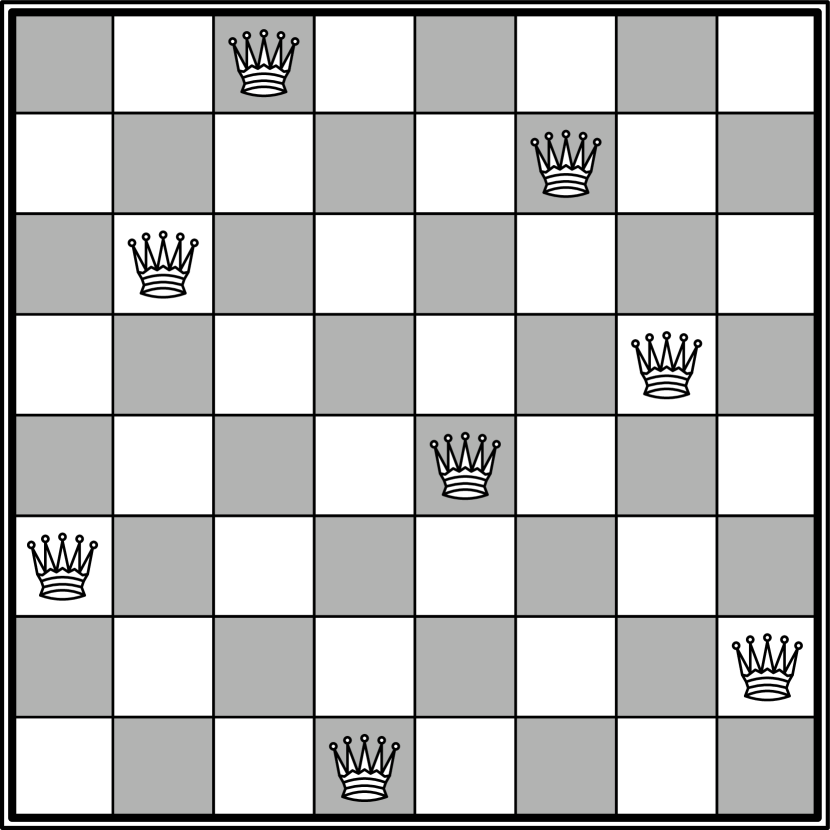
(b)

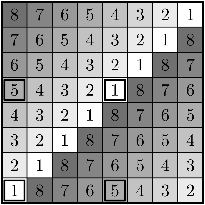
Figure 1: (a) In the $N$-queens problem, a solution is a way of placing $N$ (here $N=8$) queens on an $N\times N$ chessboard such that no two queens attack each other horizontally, vertically or diagonally. (b) The Latin square problem requires one to use $L$ different symbols (in this case $L=8$ and the symbols are $1,2,\ldots,L$) to fill an $L\times L$ table such that each symbol only occurs once in any row/column. An example of a cluster generated by the cluster algorithm (see text) is shown by the four marked cells. After it is generated, the symbols ‘1’ and ‘5’ within the cluster are exchanged.

As standard benchmark tests, many heuristic and combinatorial methods are developed to search for one or a few of their solutions, e.g., the min conflicts algorithm b.minconflict , dynamic programming b.dp and iterated map method b.itermap . However, to count all solutions is a more challenging task. The traditional approaches by a complete enumeration in general can only handle systems of a relatively small size because the number of solutions grows exponentially with the system size. To date, the largest system ($N=25$) of the $N$-queens problem contains about $2.21\times 10^{15}$ solutions according to a recent enumeration b.nqueenexact . For the Latin square problem, the largest exactly-solved system $L=11$ has about $7.77\times 10^{47}$ solutions b.latinexact .

An alternative approach is to calculate the ratio between the number of solutions of the original problem and that of a simplified problem. If we know the exact number of solutions of the simplified problem, then the number of solutions of the original problem can be deduced.

To connect the original problem (denoted as $O$) with the simpler problem (denoted as $S$), we carefully choose the problem $S$ to be a generalized version of the problem $O$ such that every solution of the problem $O$ is a solution of the problem $S$. Here, the simpler problem $S$ typically has fewer constraints, and hence more (easier-to-find) solutions. We then perform a Monte Carlo simulation in the configurational space spanned by all solutions of the problem $S$ to compute the ratio of solutions of $O$ and $S$. A convenient way to recognize a solution of the problem $O$ is to use an energy function $E$ that is nonnegative everywhere and is zero if and only if the configuration is a solution of the problem $O$.

Since the numbers of solutions of $O$ and $S$ usually differ by many orders of magnitudes as the system size increases, the ratio of the two becomes too small to be computed directly. Therefore we need a set of intermediate problems $\{S_{i}\}$, each of which is associated with a reciprocal temperature $\beta_{i}$. The $\beta_{i}$ weights each configuration according to its energy $E$ as $\exp(-\beta_{i}E)$. The weighted sum of solutions using $\beta_{i}$ is the partition function $Z_{i}=\sum\exp(-\beta_{i}E)$. Note, the partition function has an interpretation of the number of solutions in two extreme cases: the number of solutions of the problem $S$ corresponds to the partition function at $\beta=0$, and that of the problem $O$ is the partition function at $\beta\rightarrow\infty$, where only zero-energy configurations can survive. Several Monte Carlo methods were previously used to infer the partition function b.mc . However, these methods failed to be applied to large systems.

To handle large systems, we use a Monte Carlo method that directly computes the partition function b.Z , where we simultaneously sample the system at multiple temperatures by means of transitions between the temperatures. In addition to configurational space sampling under a fixed temperature $\beta_{i}$, e.g. the Metropolis algorithm b.metropolis , temperature transitions are randomly proposed from the current value $\beta_{i}$ to another one $\beta_{j}$, and accepted with a probability $\mathrm{Acc}_{\beta}=\min\{1,\exp[-(\beta_{j}-\beta_{i})E+\ln\tilde{Z}_{i}-\ln\tilde{Z}_{j}]\}$. Here, $E$ is current energy, $\tilde{Z}_{i}$ and $\tilde{Z}_{j}$ are the estimated values of the partition function at $\beta_{i}$ and $\beta_{j}$, respectively. The $\ln\tilde{Z}_{i}$’s are then dynamically converged to the actual values $\ln Z_{i}$’s through a recursive updating until an accuracy $|\ln\tilde{Z}_{i}-\ln Z_{i}|<0.10$ is reached b.Z . This accuracy guarantees a correct order of magnitude of the $\tilde{Z}_{i}$ (which is $\log_{10}\tilde{Z}_{i}=\ln\tilde{Z}_{i}/\ln{10}$). To obtain a more accurate partition function, we perform an additional run of simulation with all $\tilde{Z}_{i}$’s fixed at their final values. Practically, the final run is always much longer than all the previous updating stages; thus the cost of the updating is negligible. The statistics accumulated from the final run is used to further refine the partition function through the multiple histogram method b.multihist .

Figure 2: The numbers of solutions of the $N$-queens problem $Q_{N}$ and that of the Latin square problem $S_{L}$ versus the system size $N$ (for a Latin square $N=L\times L$). There is a simple linear relation between $\ln(N!/Q_{N})$ and $N$ while a fitting formula for $S_{L}$ is more complicated (see text). The inset shows the error of fitting the formulas to the numerical results.

For the $N$-queens problem, see Fig. 1(a), the $N$-rooks problem can serve as the problem $S$, where queens function as rooks such that they can attack each other only horizontally and vertically, but not diagonally. The problem $S$ is a trivial one: each of its solutions corresponds to a permutation of the $N$ column indices because the row constraints are satisfied by placing only one rook on each row while the column constraints are satisfied by placing rooks from different rows at different columns. Hence, there are totally $N!$ solutions for the $N$-rooks problem.

We now specify the energy function that connects the simple problem with the original one. If the diagonal $d$ has $C_{d}$ resident queens, the energy of that diagonal $E_{d}=\max\{C_{d}-1,0\}$. The energy of the whole system is a sum of the energy of all diagonals. A zero-energy configuration guarantees that no diagonal has more than one queen, and therefore is a solution of the $N$-queens problem.

We used the swap move introduced by Sosic and Gu b.swapmove to sample the configurational space. In each Monte Carlo step, we randomly choose two rows and try to swap the column indices of the queens there. Note, after a swap the horizontal and vertical constraints are still satisfied. Thus these swaps can be used to perform sampling on the configurational space of the problem $S$.

The number of solutions for systems of several typical sizes are shown in Table 1. For the largest exactly-solved system to date $N=25$ b.nqueenexact , the relative error is only $5\times 10^{-5}$. The results on small systems serve as a check of our method. Currently, there is a dispute about the number of solution for $N=24$. An alternative calculation b.n24alt gives 226732487925864 solutions instead of the value 227514171973736 used in Table 1. Our long-time simulation result $2.2751\times 10^{14}$ clearly supports the latter result. More importantly, our method can be used on much larger systems, to which one cannot apply traditional counting algorithms due to astronomically large numbers of solutions. In the largest system, there are about $1.33\times 10^{31560}$ solutions for $N=10000$ (in which case we used 82 temperatures from $\beta=9.2$ to $\beta=0$). The results on large systems are shown in Fig. 2. Our linear fitting result shows that for large systems $N>100$, the number of solutions $Q_{N}$ satisfies $\ln(N!/Q_{N})\approx 0.944001N-0.937$; the maximal fitting error is less than 0.02 in this range.

Table 1: The numbers of solutions $Q_{N}$ of the $N$-queens problems. The simulation cost are measured by sweeps (numbers of Monte Carlo steps per queen). The first six significant digits of the exact results b.nqueenexact are displayed in the last column for comparison.

$N$	sweeps	$Q_{N}$	exact value
21	$4\times 10^{10}$	$3.1468\times 10^{11}$	$3.14666\times 10^{11}$
22	$5\times 10^{10}$	$2.6910\times 10^{12}$	$2.69101\times 10^{12}$
23	$4\times 10^{10}$	$2.4234\times 10^{13}$	$2.42339\times 10^{13}$
24	$1\times 10^{11}$	$2.2751\times 10^{14}$	$2.27514\times 10^{14}$
25	$1\times 10^{11}$	$2.2080\times 10^{15}$	$2.20789\times 10^{15}$
26	$1\times 10^{11}$	$2.2320\times 10^{16}$
27	$5\times 10^{10}$	$2.3489\times 10^{17}$
28	$5\times 10^{10}$	$2.5645\times 10^{18}$
29	$5\times 10^{10}$	$2.8899\times 10^{19}$
30	$5\times 10^{10}$	$3.3731\times 10^{20}$
40	$2\times 10^{10}$	$8.273\times 10^{31}$
50	$2\times 10^{10}$	$2.456\times 10^{44}$
100	$1\times 10^{10}$	$2.392\times 10^{117}$
200	$1\times 10^{10}$	$2.041\times 10^{293}$
500	$1\times 10^{10}$	$3.219\times 10^{929}$
1000	$5\times 10^{9}$	$1.094\times 10^{2158}$
2000	$2\times 10^{9}$	$9.44\times 10^{4915}$
5000	$1\times 10^{9}$	$1.46\times 10^{14276}$
10000	$1\times 10^{9}$	$1.33\times 10^{31560}$

Next, we turn to the Latin square problem. For convenience we choose $1,2,\ldots,L$ as the $L$ different symbols to fill the $L\times L$ table. To construct a problem $S$, we remove the constraints for columns, i.e., we no longer require each symbol to occur once in a column, while retaining the constraints for rows. Thus different rows act independently. The constraints for symbols within a row being mutually different imply that each row configuration is a permutation of the $L$ symbols. Thus there are $L!$ different arrangements for each individual row, and $(L!)^{L}$ arrangements for the whole system (the problem $S$).

The energy function is the following. A symbol that is shared by two different rows on the same column contributes +1 to the total energy, i.e., $E=\sum_{i<j;~{}k}\delta(s_{ik},s_{jk})$. Here, $s_{ij}$ is the symbol at the $i$th row and $j$th column; $\delta(a,b)$ is +1 if the two symbols $a$ and $b$ are the same, zero otherwise; the two indices $i$ and $j$ enumerate over every pair of different rows, $k$ every column. A Metropolis way to sample the system is to randomly choose two columns on a row, and to try to swap their symbols. Similar to the previous case, the swaps preserve the constraints for rows, thus are qualified as a sampler of the configurational space.

However, at a low temperature, the swap becomes inefficient due to frequent rejections. For example, at the lowest temperature $\beta=8.4$ we used for the $100\times 100$ system, the average probability of accepting a swap is less than 0.01%. To overcome the difficulty, we developed a rejection-free cluster algorithm for this system and used it to generate configurational changes. The cluster algorithm is of the same spirit of its counterpart on the Ising model b.cluster . It exploits the symmetry between any two symbols $a$ and $b$, e.g., the system energy is unchanged if we exchange the two symbols in a suitable collection of rows (or a cluster).

A cluster is generated as the following. We first randomly choose two symbols $a$ and $b$ as well as a row index $i$, and add this row index $i$ into the cluster as a “seed”. We now scan the row $i$ and pick up the column $j$ where the symbol $s_{ij}$ is $a$, and search in other rows $i^{\prime}$ for the symbol $b$ at the same column $j$, i.e., $s_{i^{\prime}j}=b$ . For each row $i^{\prime}$ found, we use a probability $P_{\mathrm{add}}=1-\exp(-\beta)$ to add it into the cluster. Similarly, we pick up the column $k$ where $s_{ik}=b$, and add every other row $i^{\prime\prime}$ where $s_{i^{\prime\prime}k}=a$ to the cluster using the same probability. This process is repeated until every row in the cluster is considered. An example is shown in Fig. 1(b), where $a=1$ and $b=5$, and the bottom row is the seed. Once the cluster is formed, we exchange the symbols $a$ and $b$ within.

The number of solutions of the Latin square problem is listed in Table 2. We used the Metropolis moves for small systems, but cluster moves for large systems at low temperatures. In this way we could access large systems, as shown in Fig. 2. The size of the largest system is 100 by 100, in which there are over $10^{11710}$ solutions. In this system, we used 85 temperatures from $\beta=8.4$ to $\beta=0$. We attempted to fit the number of solutions $S_{L}$ to the formula $\ln(L!^{L}/S_{L})\approx L^{2}(0.99649+42.9721/L-35.8277/L^{2})/(1+49.6514/L+152.80/L^{2})$; the maximal fitting error is 0.03.

Table 2: The numbers of solutions $S_{L}$ of the $L\times L$ Latin square problems. One sweep is defined as the numbers of Monte Carlo steps per site. The exact results b.latinexact are displayed to the first five significant digits. We used the cluster algorithm for the last two systems.

size	sweeps	$S_{L}$	exact value
$10\times 10$	$1\times 10^{10}$	$9.988\times 10^{36}$	$9.9824\times 10^{36}$
$11\times 11$	$1\times 10^{10}$	$7.773\times 10^{47}$	$7.7697\times 10^{47}$
$12\times 12$	$1\times 10^{10}$	$3.102\times 10^{60}$
$13\times 13$	$1\times 10^{10}$	$7.500\times 10^{74}$
$14\times 14$	$1\times 10^{10}$	$1.266\times 10^{91}$
$15\times 15$	$1\times 10^{10}$	$1.728\times 10^{109}$
$16\times 16$	$1\times 10^{10}$	$2.161\times 10^{129}$
$17\times 17$	$1\times 10^{10}$	$2.804\times 10^{151}$
$18\times 18$	$1\times 10^{10}$	$4.256\times 10^{175}$
$19\times 19$	$1\times 10^{10}$	$8.354\times 10^{201}$
$20\times 20$	$1\times 10^{10}$	$2.365\times 10^{230}$
$50\times 50$	$1\times 10^{8}$	$5.67\times 10^{2250}$
$100\times 100$	$1\times 10^{7}$	$1.55\times 10^{11710}$

The heat capacity $C$ of the system shows an interesting finite-size effect. As the system size increases, the system develops two separate maxima, see Fig. 3. The anomaly of the heat capacity is a result of many frustrated low energy states. A similar phenomenon was experimentally observed in a two-dimensional antiferromagnetic system b.antiferro . Besides, the valley between the two maxima coincides with the location where the system has the maximal fraction of percolated clusters. In the cluster algorithm, a cluster is defined as percolated if it includes all rows. As shown in the inset of Fig. 3, for the $100\times 100$ Latin square, the maximum fraction 0.06 occurs at $T_{h}\approx 0.14$, where the heat capacity hits its local minimum. We now give a qualitative explanation for why the highest percolation fraction occurs at a finite temperature $T_{h}$ rather than $T=0$. At a very low temperature, each column has at most two cells with the two symbols under concern ($a$ and $b$). As the temperature is increased to $T_{h}$, a column is allowed to have more of these cells. Meanwhile $P_{\mathrm{add}}$ is not changed significantly from 1.0 (in the above example, $P_{\mathrm{add}}\approx 0.9992$ at $T_{h}$). Thus clusters are more readily spread over rows than at $T=0$. However, a further increase of the temperature decreases $P_{\mathrm{add}}$ and suppresses the growth of clusters.

Figure 3: Heat capacity $C$ per site of Latin squares versus temperature $T$. The heat capacity develops two peaks as one increases the system size. The inset shows that the valley between the two maxima of the heat capacity for the $100\times 100$ system (the solid line, the left axis) corresponds to where the fraction of percolated clusters (the dash dot line, the right axis) reaches the maximum.

In summary, we demonstrate an efficient method to count the number of solutions for the $N$-queens problem and Latin square problem. The original problem $O$ is generalized to a less-constrained problem $S$ and its partition function is calculated. We achieved a high sampling efficiency by using collective Monte Carlo moves: in the $N$-queens problem, the column indices of the queens are swapped rather than altered individually; similarly, in the Latin square problem, symbols within a row are always exchanged (the cluster move is even more collective because we also attempt to exchange symbols in different rows). These collective moves not only improve the sampling efficiency at low temperatures, but also reduce the sampling space by making the problem $S$ as close to the problem $O$ as possible. In the $N$-queens problem, the use of the swap move reduces the sampling space of the problem $S$ from $N^{N}$ solutions to $N!$ solutions, while in the Latin square problem the sampling space is reduced from $L^{L\times L}$ to $(L!)^{L}$. In the current work, the intermediate problems are associated with different temperatures. An alternative way is to compute the density of states $g(E)$ (i.e., the number of solutions with a particular energy) by a random walk on the energy space b.muca ; b.wl . However, we believe that the approach is less efficient than the one used in this work. The reason is that while the energy range is proportional to the system size $N$, it can be covered by much fewer temperatures $\sim\sqrt{N}$. Thus it takes more time to estimate the density of states than the partition function, especially for a large system. Another advantage of the current method is that it simplifies the design and application of efficient cluster algorithms. We expect the computational tool to be broadly applicable to other problems.

The authors acknowledge support from an NIH grant (R01-GM067801), an NSF grant (MCB-0818353), and a Welch grant (Q-1512).

References

- (1) S. Minton, M. D. Jonston, A. B. Philips, and P. Laird, Articial Intelligence 58 161 (1992).
- (2) R. Rivin and R. Zabih, Information Processing Letters 41 253 (1992).
- (3) V. Elser, I. Rankenburg, and P. Thilbault, Proc. Natl. Acad. Sci. USA 104 418 (2007).
- (4) N. J. A. Sloane, The On-Line Encyclopedia of Integer Sequences (OEIS) Sequence A000170.
- (5) N. J. A. Sloane, OEIS Sequence A002860.
- (6) K. Pinn and C. Wieczerkowski, Int. J. Mod. Phys. C 9 541 (1998); A. R. Lima and M. Argollo de Menezes, Phys. Rev. E 63 020106(R) (2001); K. Hukushima, Comput. Phys. Commun. 147 77 82 (2002).
- (7) C. Zhang and J. Ma, Phys. Rev. E 76, 036708 (2007).
- (8) N. Metropolis, A. W. Rosenbluth, M. N. Rosenbluth, A. H. Teller, and E. Teller, J. Chem. Phys. 21, 1087 (1953).
- (9) A. M. Ferrenberg and R. H. Swendsen, Phys. Rev. Lett. 61 2635 (1988); 63 1195 (1989).
- (10) R. Sosic and J. Gu, ACM SIGART Bulletin 1 7 (1990).
- (11) N. J. A. Sloane, OEIS Sequence A140393.
- (12) R. H. Swendsen and J. S. Wang, Phys. Rev. Lett. 58 86 (1987); U. Wolff, ibid. 62 361 (1989).
- (13) D. S. Greywall and P. A. Busch, Phys. Rev. Lett. 62 1868 (1989); K. Ishida, M. Morishita, K. Yawata, and H. Fukuyama, ibid. 79 3452 (1997).
- (14) B. Baumann, Nucl. Phys. B 285, 391 (1987); B. A. Berg and T. Neuhaus, Phys. Rev. Lett. 68, 9 (1992); B. A. Berg and T. Celik, ibid. 69, 2292 (1992); B. A. Berg and W. Janke, ibid. 80, 4771 (1998).
- (15) F. Wang and D. P. Landau, Phys. Rev. Lett. 86 2050 (2001).