Measuring the undetectable:
Proper motions and parallaxes of very faint sources

Abstract

The near future of astrophysics involves many large solid-angle, multi-epoch, multi-band imaging surveys. These surveys will, at their faint limits, have data on large numbers of sources that are too faint to be detected at any individual epoch. Here we show that it is possible to measure in multi-epoch data not only the fluxes and positions, but also the parallaxes and proper motions of sources that are too faint to be detected at any individual epoch. The method involves fitting a model of a moving point source simultaneously to all imaging, taking account of the noise and point-spread function in each image. By this method it is possible to measure the proper motion of a point source with an uncertainty close to the minimum possible uncertainty given the information in the data, which is limited by the point-spread function, the distribution of observation times (epochs), and the total signal-to-noise in the combined data. We demonstrate our technique on multi-epoch Sloan Digital Sky Survey (SDSS) imaging of the SDSS Southern Stripe. We show that with our new technique we can use proper motions to distinguish very red brown dwarfs from very high-redshift quasars in these SDSS data, for objects that are inaccessible to traditional techniques, and with better fidelity than by multi-band imaging alone. We re-discover all 10 known brown dwarfs in our sample and present 9 new candidate brown dwarfs, identified on the basis of significant proper motion.

1 Introduction

There are many multi-epoch imaging surveys in progress or coming up, which will, among other things, deepen our image of the sky and provide information on source variability and proper motions. These surveys include the SDSS Southern Stripe (Abazajian et al., 2009), the Dark Energy Survey, PanSTARRS, LSST, and SNAP. These surveys promise proper-motion precisions for well-detected sources on the order of $\mathrm{mas}\,\mathrm{yr}^{-1}$ over large parts of the sky. For context, a typical halo star at a distance of $10~{}\mathrm{kpc}$ moving at a transverse heliocentric speed of $100~{}\mathrm{km}\,\mathrm{s}^{-1}$ has a proper motion of $2~{}\mathrm{mas}\,\mathrm{yr}^{-1}$, and a typical disk star at $100~{}\mathrm{pc}$ and $10~{}\mathrm{km}\,\mathrm{s}^{-1}$ has a proper motion of $20~{}\mathrm{mas}\,\mathrm{yr}^{-1}$. These surveys therefore have the capability of revolutionizing our view of the Galaxy and of the Solar neighborhood.

In most conceptions of a proper-motion measurement, one imagines measuring the position of a source in each of several images, taken at different times. A linear trajectory is fitted to the positions, relative to some reference frame or set of fixed sources or sources with well measured proper motions. In its most straightforward form, this method only works for sources bright enough to be detected independently at every epoch—or at least most epochs. In a multi-epoch survey like the SDSS Southern Stripe, which has $\sim 70$ epochs (Abazajian et al., 2009), this limits the sources with measured proper motions to a small subset of all sources detectable in the combined data, since the combined data reach $\sim 2.3~{}\mathrm{mag}$ fainter than any individual epoch; for typical source populations this represents increases in population size by factors of $5$ to $25$ at any given signal-to-noise threshold. In this paper we present a methodology for measuring in multi-epoch imaging the proper motions of sources too faint to detect at any individual epoch.

There are several different technical regimes for these faint-source proper-motion measurements. In the “easy” regime, the sources of interest move a distance smaller than or comparable to the point-spread function width over the duration of the multi-epoch survey. In this regime, the sources are easy to detect in the co-added image, even without taking account of their proper motions; proper motions can be determined from processing the individual epoch images after detection in the co-added image. There is a “difficult” regime in which the sources of interest move substantially more than the width of the point-spread function over the duration of the survey. In this regime, the source will not appear at high significance in the co-added image if it does not appear at high significance at any epoch, because its different appearances in the different individual-epoch images do not overlap. In principle, the difficult regime can be addressed by brute force with large computing resources. In the context of outer Solar-System bodies, brute-force search in the narrow range of expected motions is feasible (for example, Bernstein et al. 2004; Fuentes et al. 2008). In this paper, we consider only the easy regime.

Modeling the data:

The traditional method for measuring a stellar proper motion with a set of images taken at different times is as follows: Detect the star at each observed epoch; measure its centroid (by, for example, finding the peak or first moment of the flux) at each observed epoch; and fit a linear motion to the measured positions and times. This procedure obtains a proper motion, but it puts an unnecessary requirement on the data: that the star be detectable at every epoch. It also puts an unnecessary burden on the data analyst: it requires decision making about detection and centroiding of the stars at each epoch, decisions that matter at low signal-to-noise, or when faced with data issues such as bad pixels or strong variations in noise from pixel to pixel.

Our new approach is to model all individual-epoch images simultaneously with a single point source that is permitted to have a non-zero parallax and proper motion. This approach combines the individual-image positional measurement and the determination of the parallax and proper motion, and determines all of these simultaneously by making a statistically “good” model of the union of all the data.

In any well-understood imaging survey, each image will have a per-pixel noise model, photometric calibration parameters, and a model of the point-spread function. In any sufficiently small patch of the sky, if the foreground-subtracted intensity in that patch is dominated by a small number of point sources, it is possible to make an accurate model of all of the pixels in the data set that contribute signal to that small patch. In this model of the patch, the fluxes, angular positions, parallaxes, and proper motions of the stars in the patch are simply parameter values in the well-fitted models. In other words, we are assuming that it is possible to model the set of pixels (from all of the images) that contribute to the patch with a $6N$-dimensional model that consists of a set of $N$ moving point sources.

The proper motions determined by image modeling have several advantages over those determined by the traditional method: They require fewer decisions about measurement techniques (although they do require a good model of the data, including point-spread function); they use all of the information in all of the pixels, not just those pixels involved in traditional centroiding; they gracefully handle missing data due to bad pixels or cosmic rays (assuming the bad pixels have been flagged); they require the investigator to make explicit the assumptions about the physical properties of the image and the noise; they can be made to properly propagate pixel-value uncertainties into parameter uncertainties (in this case, proper motion uncertainties); they are the result of optimization of a well-justified scalar objective function (in this case the likelihood). Most importantly for what follows, they can be determined in data sets in which the stars are not well detected at any individual epoch, but only appear in the combination of the images. In a data set with $\sim 70$ similar epochs (such as the SDSS Southern Stripe), this corresponds to an increase in the number of available targets by factors of $5$ to $25$ (assuming source populations double to quadruple with each magnitude of depth).

Here we propose, build, test, and use an image-modeling system for the determination of stellar proper motions. We show that it can work down to low signal-to-noise ratios and that it makes measurements in real data that fully exploit the information available. We also use it to discover interesting new astrophysical sources. An approximation to the technique used here has been used previously in the Solar System literature (Bernstein et al., 2004).

Proper-motion and parallax uncertainties:

Consider a well-sampled image $i$ with a point-spread function of full width at half maximum ${\theta_{\mathrm{FWHM}}}_{i}$. The signal-to-noise at which the flux of a point source can be measured, ${[s/n]}_{i}$, is the sum in quadrature of the signal-to-noise contributions from pixels within the point-spread function. A point source measured with signal-to-noise ${[s/n]}_{i}$ in a single image can be centroided with (RMS) uncertainty $\sigma_{\theta,i}$ of

$$\sigma_{\theta,i}\approx\frac{{\theta_{\mathrm{FWHM}}}_{i}}{{[s/n]}_{i}}\quad;$$ (1)

details such as the shape of the point-spread function introduce factors of order unity (King, 1983).

If we have $N$ such images spanning some time interval, we might hope to obtain a proper motion estimate with uncertainty $\sigma_{\mu}$ limited by the point-spread function, the time interval, and the total signal-to-noise

$${[s/n]}_{\mathrm{total}}^{2}=\sum_{\mathrm{images}\ i}{[s/n]}_{i}^{2}$$ (2)

in the combination of all the images (we have assumed here that the images $i$ are all independent). The relevant time “interval” is not the total time spanned by the data but rather $\delta_{t}\equiv\sqrt{\mathrm{Var}({t})}$, the standard deviation (root variance) of the times; the best possible proper-motion estimates will have uncertainties

$$\sigma_{\mu}\approx\frac{{\theta_{\mathrm{FWHM}}}}{\delta_{t}\,{[s/n]}_{\mathrm{total}}}\quad,$$ (3)

where properly ${\theta_{\mathrm{FWHM}}}$ is the square-signal-to-noise weighted mean point-spread function full width at half maximum, and $\delta_{t}$ is the square root of the square-signal-to-noise-weighted variance of the times at which the individual epoch images were taken.

By a similar argument, we hypothesize that the best possible parallax estimates will have uncertainties

$$\sigma_{\pi}\approx\frac{{\theta_{\mathrm{FWHM}}}}{\delta_{\lambda}\,{[s/n]}_{\mathrm{total}}}\quad,$$ (4)

where $\delta_{\lambda}$ is the square root of the square-signal-to-noise-weighted variance of the trigonometric functions of the ecliptic longitude $\lambda$ of the Sun (time of year in angle units):

$$\delta_{\lambda}^{2}\equiv\sigma_{\cos\lambda}^{2}+\sigma_{\sin\lambda}^{2}\quad.$$ (5)

Essentially, $\delta_{\lambda}$ describes how well the parallactic ellipse is sampled; an ideal survey for parallax measurements will have $\delta_{\lambda}\approx 1$.

Disk stars move with respect to one another at velocities of $\sim 30\,\mathrm{km}\,\mathrm{s}^{-1}$ (Dehnen & Binney, 1998; Hogg et al., 2005), that is, on the same order as the velocity of the Earth around the Sun. In a multi-epoch survey spanning a small number of years (such as the SDSS Southern Stripe), $\delta_{t}$ is of order unity, so for disk stars the parallax and proper motion signal-to-noise ratios ought to be comparable in magnitude. However, most surveys sample ecliptic longitude $\lambda$ poorly, because of season and scheduling constraints; therefore $\delta_{\lambda}$ is usually substantially less than unity, so the signal-to-noise of parallax is smaller than that of proper motion.

2 Method

The goal is to measure the proper motions and parallaxes of sources detected in multi-epoch data. We start with a catalog of detections from a co-addition of the multi-epoch data (co-added at zero lag or under an assumption that the sources are static). These detections serve as “first-guess” positions for sources in the imaging. We measure the properties of these sources by building models of all the individual images, at the pixel level, so that each model “predicts” every pixel value in every image at every epoch.

Some of the candidate sources will not be point sources but rather resolved galaxies, and others will not be astronomical sources but will be caused by artificial satellites or imaging artifacts. We fit three qualitatively different models, described below. One is of a moving point source, one is of an extended galaxy, and one is of a general transient or artifact. For each model, “fitting” constitutes optimizing a scalar objective, which is the logarithm of the likelihood under the assumption that the per-pixel noise is Gaussian with a known variance in each pixel. Under the Gaussian assumption, we can use the different values of the log likelihood to perform a hypothesis test based on likelihood ratios. This hypothesis test distinguishes point sources from extended galaxies and transients and artifacts. The parameters of the best-fitting model are the “measurements” of the source.

Nothing in what follows fundamentally depends on the assumption of Gaussian noise. Data with Poisson errors, for example, can be analyzed the same way but with the objective function changed to the logarithm of the Poisson likelihood. Indeed, any noise model can be accomodated, though possibly at the expense of computational simplicity.

In detail, for each source, we have $N$ small images (patches of what is presumed to be a much larger imaging data set) $i$ taken at times $t_{i}$, and we assume that each image has reasonable photometric calibration, a noise estimate in each pixel (assumed Gaussian, but that could be relaxed in what follows), and correct astrometric calibration or world coordinate system (WCS) fixed to an astrometric $({\mathrm{RA}},{\mathrm{Dec}})$ reference frame. From a co-added image made from all $N$ single-epoch images we have been given a candidate (“first-guess”) position $({\mathrm{RA}}_{j},{\mathrm{Dec}}_{j})$ for each source $j$.

point-source model

The first of the three models is that of a point source, moving in space and a finite distance from the Solar System. This point source is assumed to have a constant flux $S_{j}$, a position $({\mathrm{RA}}_{j},{\mathrm{Dec}}_{j})$ at some standard epoch, a parallax $\pi_{j}$ and a proper motion $\bm{\vec{\mu}}_{j}=({\mu_{\alpha}}_{j},{\mu_{\delta}}_{j})$. In this model and the models to follow, we assume that the sky level has been correctly fitted and subtracted from the images, or else that sky errors are not strongly covariant with errors in the model parameters. In fitting this model, we find the six-dimensional quantity $(S_{j},{\mathrm{RA}}_{j},{\mathrm{Dec}}_{j},\pi_{j},{\mu_{\alpha}}_{j},{\mu_{\delta}}_{j})$ that optimizes the scalar objective.

Given the times $t_{i}$ and WCS of the images, any point-source parameter set $(S_{j},{\mathrm{RA}}_{j},{\mathrm{Dec}}_{j},\pi_{j},{\mu_{\alpha}}_{j},{\mu_{\delta}}_{j})$, specifies the pixel position of point source $j$ in each image $i$. This position and the (possibly position-dependent) point-spread function model for image $i$ permits construction of a pixel-for-pixel model of source $j$ as it ought to appear in image $i$.

If we had multi-band imaging (the tests below are on are on single-band images), the flux $S_{j}$ becomes a set of fluxes $S_{kj}$, one for each bandpass $k$. In principle, precise fitting is complicated by the existence of differential refraction for sources with extreme colors, so there are relationships among the fluxes $S_{kj}$, positional offsets, and the airmass or altitude of the observations. In the tests below, we are working far enough to the red that there are no differential refraction issues at the relevant level of precision.

Although we have assumed non-varying flux in our model, we should still be able to detect and measure moving sources with varying flux. We have not investigated this question, but we expect that our method would produce a flux estimate of approximately the mean flux measured at the available epochs, and that the point-source model would be preferred over the transient model, since the objective function is convex.

galaxy model

Our model of a resolved galaxy is a Gaussian distribution of flux with an elliptical covariance parameterized by its radius $r_{j}$, eccentricity $e_{j}$, angle $\theta_{j}$ and total flux $S_{j}$. For each image, this Gaussian model is convolved with that image’s particular point-spread function to make a seeing-convolved galaxy model. This seeing-convolved Gaussian galaxy model is not a realistic galaxy model, but it is good enough for distinguishing resolved and unresolved sources at the faint limit, which is sufficient here. Again, if we had multi-band imaging, the flux $S_{j}$ would be replaced by a set of fluxes $S_{jk}$.

junk model

Our model of a transient or imaging artifact is that there is nothing but noise in all but one of the images, and that one “junk” image contains many bright pixels. We compute this model trivially by computing the chi-squared ($\chi^{2}$) contribution for each image under the assumption that there is no flux in the image at all. The image with the largest $\chi^{2}$ contribution is judged to be the “junk” image and is discarded. In order to keep the number of $\chi^{2}$ contributions constant, we replace the “junk” image $\chi^{2}$ by the median of the $\chi^{2}$ contributions of the remaining images.

scalar objective optimization

The choices of model, scalar objective, and optimization methodology can all be made independently. For the objective function the natural choice is the $\chi^{2}$ difference between the model and the data taken over all the pixels that are close to the first-guess position in all $N$ images. This objective is analogous to a logarithm of a likelihood ratio; it is exact if the noise in the image pixels is Gaussian and independent, with known variances (which can vary from pixel to pixel). For optimizing this objective function, we use the Levenberg-Marquardt method (Levenberg, 1944; Marquardt, 1963).

hypothesis test

In the approximation that the noise is Gaussian, the best fits for each of the three models can be compared via the best-fit values of the $\chi^{2}$ scalar objective. If the three models are equally likely a priori and if they have the same number of degrees of freedom, then one model is confidently preferred over another if it has a best-fit $\chi^{2}$ value smaller by an amount $\Delta\chi^{2}\gg 1$. Of course the models are not equally likely a priori, but for for the vast majority of sources, the differences in $\chi^{2}$ are so large that no reasonable prior would change the results of our hypothesis test.

Note that there is some degeneracy in our models: a galaxy model with zero radius and a star model with zero proper motion and parallax produce exactly the same predictions, and thus our hypothesis test cannot distinguish them. This could be remedied by placing prior probabilies over the model parameters—for example, penalizing tiny galaxies—but since we are not concerned with the region of parameter space where this occurs, we have not done this.

Rather than explicitly including a junk model, we could instead place a threshold on the likelihood of the star and galaxy models: junk data will be poorly fit by the star and galaxy models and thus will have tiny likelihood. In general we have found that image sets for which the junk model is preferred clearly contain artifacts or transients; the method is not sensitive to the details of the junk model.

jackknife error analysis

In principle, the region in parameter space around the best-fit point where $\chi^{2}$ is within unity of the minimum provides an estimate of the uncertainties in the fitted parameters. However, this estimate is only good when the model is a good fit; many error contributions in real data come from source variability, poorly known data properties (such as pixel uncertainty or point-spread-function estimates that are in error) and unflagged artifacts in the data. For this reason, we use (and advocate) a “jackknife” technique for error analysis.

The jackknife technique is to perform the analysis on the $N$ subsets of the $N$ images created by leaving one image out. The complete fit of the three models is performed on each of the $N$ leave-one-out subsets and parameters are measured. The uncertainty estimate $\sigma_{p}$ for any fitted parameter $p$ is related to the $N$ leave-one-out measurements $p_{i}$ (made leaving out image $i$) by

$$\sigma_{p}^{2}=\frac{N-1}{N}\,\sum_{i}\left(p_{i}-\left<{p}\right>\right)^{2}\quad,$$ (6)

where $\left<{p}\right>$ is the mean of the leave-one-out measurements $p_{i}$. The jackknife technique automatically marginalizes the error estimates over the other parameters, and provides a properly marginalized estimate of any multi-parameter covariance matrix by the generalization of equation (6) in which the square is changed into the $d\times d$ matrix outer product of the “vectors” made from the $d$ parameters for which the covariance matrix is desired. Of course when $d$ is large, the jackknife will not accurately sample all degrees of freedom available in the covariance matrix, but provided $N$ is large enough, it will sample the dominant eigenvectors (the principal components).

Implementation notes

Our code is implemented in Python and uses the Django web framework, which provides powerful database and web server integration. This allows us to quickly and easily manage and visualize the data and results. Combined with the scientific data analysis packages scipy and numpy and the plotting package matplotlib, this yielded a powerful software development environment.

For optimization, we use the Levenberg-Marquardt implementation levmar (version 2.2; Lourakis 2004) with Python bindings pylevmar (revision 313; Tse 2008). In this Python environment, analysis takes on the order of seconds for each source (30 epochs, $15\times 15$ images), but this could be sped up substantially by implementing some of the core operations in C.

3 Tests on real data

For test data, we make use of the SDSS Southern Stripe (SDSSSS), a multi-epoch survey undertaken as part of SDSS-II (Adelman-McCarthy et al., 2008; Abazajian et al., 2009). The SDSSSS data are part of The Sloan Digital Sky Survey (Gunn et al., 1998; York et al., 2000); it involves $ugriz$ CCD imaging of $\sim 250~{}\deg^{2}$ on the Equator in the southern Galactic cap. All the SDSSSS data processing, including astrometry (Pier et al., 2003), source identification, deblending and photometry (Lupton et al., 2001), and calibration (Smith et al., 2002; Padmanabhan et al., 2008) are performed with automated SDSS software.

The SDSSSS data have been found to have a small astrometric drift (Bramich et al., 2008), because astrometric calibration was performed at a single, slightly inappropriate epoch (Pier et al., 2003). This drift, for which we are making no correction, is at the $10~{}\mathrm{mas}\,\mathrm{yr}^{-1}$ level; at the precision of this study it does not change any of the conclusions below.

In general, the hypothesis test we perform requires that the variance of the noise be properly estimated on a pixel-by-pixel basis. These are based on an SDSS imaging noise model, with the adjustment that pixels that have been corrupted by cosmic rays or other defects are given infinite variances (vanishing contribution to $\chi^{2}$). Occasionally there are unidentified cosmic rays in the data. These lead to localized regions with very large contributions to $\chi^{2}$. When one of these noise defects appears in the data near one of the targets, it sometimes causes a source which is truly a galaxy or a star to be assigned “junk” status. After by-eye inspection of cutouts, we estimate this rate to be on the order of $<0.5$ percent for this data source; the rate of such problems increases with the number of epochs and the image cut-out size (the total number of pixels in the fit).

For some of the sources we have UKIRT Infrared Deep Sky Survey (UKIDSS; Lawrence et al. 2007) data. UKIDSS uses the UKIRT Wide Field Camera (Casali et al., 2007) with the infrared photometric system described by Hewett et al. (2006), and automated data processing and archiving (Irwin et al., 2008; Hambly et al., 2008). The UKIDSS data used here comes from the fourth data release.

Very red point sources in deep optical imaging—for example, $z$-band-only sources in the multi-epoch SDSS Southern Stripe—include both very cool dwarfs and very high redshift quasars. In principle these can be distinguished with parallax and proper-motion estimates. For this reason, we performed a test on $z$-only point sources in the SDSS Southern Stripe. The parent sample is point sources from the SDSSSS “Co-add Catalog” (J. Annis et al., in preparation) that have $[i-z]>2~{}\mathrm{mag}$ and $[r-z]>2~{}\mathrm{mag}$. This criterion selects quasars at $5.8\lesssim z\lesssim 6.5$ as well as cool dwarfs with spectral types ranging from mid-L to T (Fan et al. 2001 and references therein). Hotter brown dwarfs, stars, and lower-redshift quasars have significant emission in the $i$ band, giving them bluer $i-z$ colours, while the emission features of cooler dwarfs and higher-redshift quasars lie mostly redwards of the SDSS $z$ bandpass.

The Co-add Catalog uses the asinh magnitude (or “luptitude”) scale (Lupton et al., 1999), so it is possible to select objects based on color even for objects that are not detected in one of the bands. The version of the Co-add Catalog we are using is from SDSS Data Release 7 (DR7), and includes $20$ to $40$ epochs over $\sim 250~{}\deg^{2}$.

Since we are interested in distinguishing cool brown dwarfs from high-redshift quasars, we require $\sigma_{\mu}$ to be small (equation 3). We therefore cut our parent sample to have $z<21~{}\mathrm{mag}$, leaving roughly 150 sources. This cut allows us to reach, with moderate signal-to-noise, slightly fainter sources than are detectable in the single-epoch images. In a future paper, we plan to relax this cut, which should yield considerably more brown dwarf candidates at smaller signal-to-noise levels. Of our 150 parent candidates, some turn out to be caused by an imaging artifact or transient in one of the $N$ epochs, and some turn out to be galaxies or stars with mis-measured colors because of data artifacts or inaccuracies in deblending nearby objects.

Each of the catalog sources has a nominal position and a $z$-band magnitude in the Co-add Catalog. For each $z$-only source, we cut out $15\times 15~{}\mathrm{pix}^{2}$ patches of every SDSS image at the nominal position. For each tiny image, we construct a tiny local world-coordinate-system description of the astrometric calibration of that patch using the SDSS pipeline astrometric calibration. We subtract the local value of a smoothly fit sky level (M. Blanton, in preparation) and multiply each tiny image by a constant, based on the pipeline calibration information, to place it on a common photometric calibration scale in intensity units (energy per unit solid angle per unit area per unit time per unit frequency). To the SDSS pipeline-reconstructed point-spread function (PSF) in each tiny image we fit a single-Gaussian approximate model, which is not a good fit to the PSF at high precision, but which is sufficient for modeling sources at low signal-to-noise.

In this work, we create the $15\times 15~{}\mathrm{pix}^{2}$ cutouts from the same $20$ to $40$ epochs that are used in the Co-add Catalog; in future work we plan to use the $\sim 70$ epochs that have become available in DR7.

We chose $15\times 15~{}\mathrm{pix}^{2}$ patches so that a source with proper motion of $\sim 0.5~{}\mathrm{arcsec}\,\mathrm{yr}^{-1}$ would remain in the patch. Our method still works if the source leaves the patch—indeed, our fastest-moving candidate does this—but we gain no information from the epochs in which the source has left the patch, so the signal-to-noise of our parameter estimates will be less than optimal when this happens. We could choose to use larger cutouts; the only difficulty is that if the patch contains more than one source, our model will try to explain the brightest source (because this will decrease $\chi^{2}$ the most). This could perhaps be remedied by adding a prior on the source position, but since the SDSSSS data are from well below the galactic equator, stellar density is low and we have not found this to be necessary. Alternatively, in cases where the source leaves the original patch we could produce new cutouts that track the source motion.

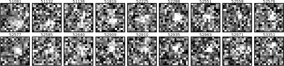
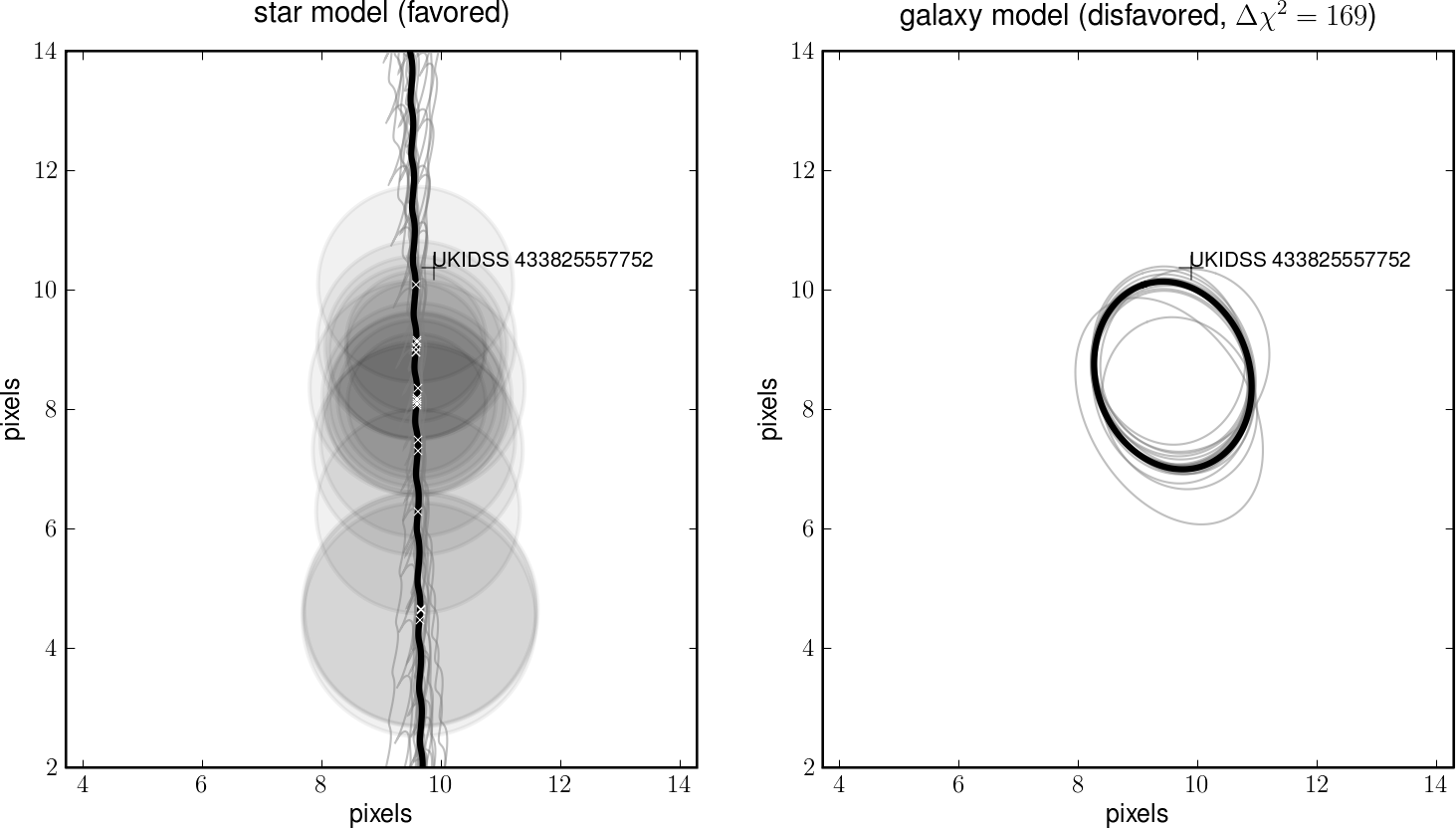
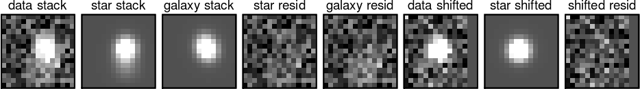
Figure 1: [caption on next page]

Figures 1 through 4 illustrate our approach by showing the results of the (moving) point-source and (static) galaxy model fits to four sources in the the SDSSSS data. In these figures we show all the individual $15\times 15$ images from the individual epochs, and the best-fit point-source and galaxy parameters. In these figures, we visualize the distribution of acceptable parameters around the best-fit values through sampling. We also show mean images and mean residual maps in the static and moving coordinate systems. These figures demonstrate heuristically that the hypothesis test is effective at separating sources of different types, even when the source is not apparent at high signal-to-noise at any individual epoch.

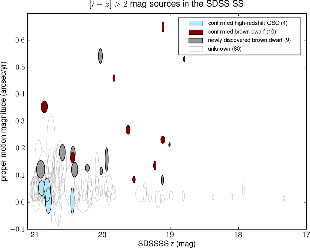
Figure 5: Proper motion magnitude (angular speed) as a function of SDSSSS Coadd Catalog $z$-band magnitude for $[i-z]>2$ mag sources in the SDSS Southern Stripe that are preferentially described as point sources (by our $\chi^{2}$ hypothesis test). The uncertainty regions are shown as transparent ellipses. The spectroscopically confirmed high-redshift quasars (Jiang et al., 2008) and brown dwarfs (Fan et al., 2000; Geballe et al., 2002; Hawley et al., 2002; Berriman et al., 2003; Knapp et al., 2004; Chiu et al., 2008; Metchev et al., 2008) are shown in color. Every one of the brown dwarfs has a significantly measured proper motion; none of the quasars do. Other brown-dwarf candidates are clearly visible as significant movers (see also Table 1). Note that the single-epoch detection limit is approximately $z=20.5~{}\mathrm{mag}$ in good seeing conditions.

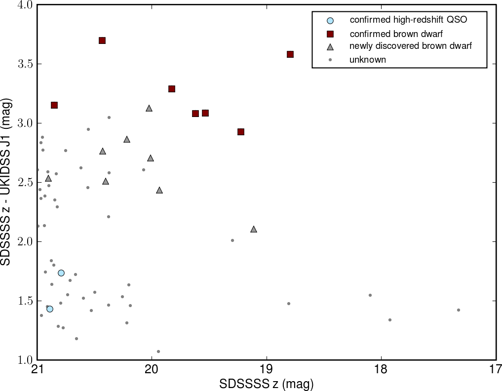
Figure 6: UKIDSS and SDSSSS $[z-J]$ color plotted against SDSSSS $z$-band magnitude, for the sources in Figure 5 that are detected in the UKIDSS $J$ band. All of the significantly-moving objects have the very red $[z-J]$ colors of brown dwarfs; the likely brown dwarfs could have been identified by their proper motions and SDSSSS Coadd Catalog colors alone. Note that the $z$ magnitude is in the AB system, while the $J$ magnitude is Vega-based.

In Figure 5 we show the overall results from application of our techniques to the $[i-z]>2$ mag sources in the SDSSSS: We show proper-motion measurements and jackknife estimates of our uncertainties as a function of $z$-band magnitude. Known quasars and brown dwarfs are marked. Our measurements clearly separate the known quasars and brown dwarfs on the basis of proper motion alone. All known brown dwarfs in the sample obtain significant non-zero proper motion measurements, and all known high-redshift quasars in our sample obtain proper motion measurements consistent with zero. The sources in our sample that have significant motions and have not been previously identified as brown dwarfs are our new brown dwarf candidates. In Figure 6 we show the UKIDSS and SDSS $[z-J]$ colors of the sources for which we have UKIDSS $J$ measurements, with the known brown dwarfs and quasars and our new brown dwarf candidates marked. Many of the sources in these Figures are undetectable (or not detectable reliably) at individual epochs; the single-epoch $5$-sigma detection limit is roughly $z=20.5~{}\mathrm{mag}$ in good seeing conditions (Abazajian et al., 2009).

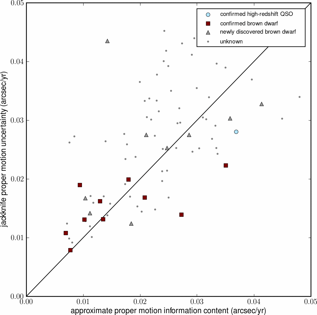
Figure 7: Comparison of the jackknife-estimated proper-motion uncertainties to “best-case” values estimated from general principles of information in the imaging: The information estimate is the mean (square-signal-to-noise-weighted) imaging point-spread function FWHM divided by the signal-to-noise of the flux measurement (taken to be a proxy for the total detection signal-to-noise), divided by the root-variance of the time span. This figure shows that the measurements are roughly as precise as they can be, given the information content of the set of images; see equation (3).

In Figure 7, our jackknife estimates of our measurement uncertainties are compared to approximate estimates of the total information content in each source’s data set, made with an approximation to equation (3). If our uncertainty estimates are correct (as we demonstrate that they are, below), this shows that we come close to attaining the accuracy available.

4 Tests on artificial data

To demonstrate that our jackknife error estimates are reasonable, and that our code is optimizing the models correctly, we performed some tests on synthetic data. We selected a subset of the SDSSSS candidate objects for which we found reasonable fits to a moving point source model. For each candidate, we generated a stack of images by generating, for each image in the original stack, the image predicted by our point-source model, given the WCS, point-spread function, time, and noise amplitude of the image. This is a good test set because it has the same imaging properties as the original data and the same distribution of point-source parameters as the sources we want to be able to discover. Since the synthetic images are generated using our image model, this test shows how our algorithm would perform if our modeling assumptions were exactly correct.

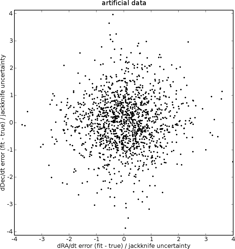
Figure 8: Accuracy of jackknife uncertainty estimates for fits to artificial data made with known point-source properties. Errors in fit parameters (fit minus true) have been divided by jackknife uncertainties. The artificial data sets have identical imaging properties (noise amplitude, WCS, and PSF) to SDSS Southern Stripe sources, but contain artifical images made with point sources with true positions, fluxes and motions derived from the data as described in the text. The cloud of points is centered near $(0,0)$, is circularly symmetric, and appears roughly Gaussian: our estimates are unbiased, uncorrelated, and have the expected magnitude and distribution of error.

After running our optimization code on these synthetic images, we compare our errors—the differences between the true and estimated moving-point-source parameters—to the jackknife estimates of our uncertainties. In Figure 8 we show that the errors are consistent with the uncertainty estimates. This shows that when our assumptions about the data are correct, we do measure the proper motions as accurately as our jackknife errors indicate.

5 Discussion

We have shown that straightforward image modeling permits the measurement of apparent motions, especially the proper motion and parallax of a source in multi-epoch data, even when the source is too faint to be reliably detected or centroided at any individual epoch. The results of this project are not surprising; indeed what is surprising is how rarely the measurements of stellar motions are made by comprehensive data modeling.

We demonstrated the technique on real and artificial data. In the process of performing these tests we showed that spectrosopically confirmed quasars and brown dwarfs can be perfectly distinguished with proper motions measured by this technique. Working without proper motions, but with Co-add Catalog sources and a significant amount of near-infrared imaging follow-up, a group has followed up the $z$-only sources most likely to be high-redshift quasars (Chiu et al., 2008; Jiang et al., 2008). This project, even after infrared imaging, found—after expensive spectroscopic follow-up—that some of the high-redshift quasar candidates selected on the basis of visible and near-infrared imaging are in fact nearby brown dwarfs. We have shown that all of these spectroscopically confirmed brown dwarfs have significantly measured ($>5$ sigma) non-zero proper motions by the technique shown here (and are reported in Table 1). None of the spectroscopically confirmed high-redshift quasars do. Use of this technique could have been used to substantially increase the efficiency of either quasar or brown-dwarf searches in this data set.

In performing this demonstration, we have independently identified all 10 known brown dwarfs (Fan et al., 2000; Geballe et al., 2002; Hawley et al., 2002; Berriman et al., 2003; Knapp et al., 2004; Chiu et al., 2008; Metchev et al., 2008) in our parent sample, and we have discovered 9 new candidate brown dwarfs, presented in Table 1. Based on our analysis, these objects have a high probability of being brown dwarfs. It would be desirable to separate disk dwarfs from halo dwarfs—the fastest angular movers tend to be halo members (for example, Lépine et al. 2003)—but the time cadence of the SDSSSS data is such that parallaxes are not measured well. Two of the dwarfs we rediscover—2MASS J010752.42+004156.3 and 2MASS J020742.84+000056.4—have previously measured parallaxes (Vrba et al., 2004); the measurements are consistent with our upper limits.

Our tests show that the uncertainty in the proper-motion measurement made by image modeling is consistent with the best possible uncertainties given the angular resolution and photometric sensitivity of the combination of all images in the multi-epoch data set. These tests effectively show that such measurements can be made for objects that are fainter than those available to traditional methods that require source detection at every epoch. In imaging with $N$ equally sensitive epochs, we are able to measure objects that are fainter by $\Delta m$ magnitudes:

$$\Delta m = -\log_{2.5}({[s/n]}_{i})+\log_{2.5}({[s/n]}_{\mathrm{total}})$$ (7)

$$= \log_{2.5}(\sqrt{N})$$ (8)

$$\sim 0.55\,\log N~{}\mathrm{mag}\quad.$$ (9)

This advantage amounts to $1~{}\mathrm{mag}$ for surveys with $6$ similar epochs, and $1.6$ to $2.0~{}\mathrm{mag}$ in data with $20$ to $40$ epochs (such as the data used here). In the $\sim 70$ epochs available in SDSS DR7, it reaches $2.3~{}\mathrm{mag}$. Several of the high-redshift quasars and brown dwarfs analyzed in this study were only detectable in the combination of all of the multi-epoch images.

The depth advantage of image modeling is most dramatic in surveys with very large numbers of epochs, as is expected for LSST. In general the number of interesting sources is a strong function of depth (factors of $2$ to $4$ per magnitude), so the “reach” of the image-modeling technique is a strong function of the number of epochs.

One limitation of the work presented here is that we used the zero-proper-motion image “stack” for source detection and therefore will only have in the candidate list objects with small proper motions. Faint stars and dwarfs with proper motions large enough that they move the width of the PSF between epochs, or some significant fraction of that, are harder to find, because they don’t appear in the stack at much higher signal-to-noise than they appear in any individual-epoch image. In future work we hope to address the detection and measurement of these fast-moving but very faint sources. Approximations have been executed in the search for Solar System bodies (for example, Bernstein et al. 2004). Certainly a reliable system for discovery in this regime would have a big impact on future surveys like PanSTARRS and LSST.

Name	RA	Dec	flux	parallax	dRA/d$t$	dDec/d$t$	notes
	deg	deg	$s/n$	arcsec	arcsec yr-1	arcsec yr-1
SDSS J001608.47$-$004302.9	$4.03537$	$-0.71733$	$46.4$	$+0.007\pm 0.058$	$+0.134\pm 0.015$	$-0.020\pm 0.007$	2 U BD
SDSS J005212.29+001216.0	$13.05131$	$+0.20465$	$29.6$	$-0.053\pm 0.069$	$-0.165\pm 0.014$	$-0.211\pm 0.010$	2 U BD
SDSS J010407.68$-$005329.1	$16.03195$	$-0.89128$	$59.1$	$-0.041\pm 0.068$	$+0.460\pm 0.010$	$-0.017\pm 0.008$	2 U BD
SDSS J010752.59+004156.0	$16.96899$	$+0.69905$	$59.0$	$+0.044\pm 0.070$	$+0.644\pm 0.014$	$+0.085\pm 0.013$	2 BD
SDSS J020333.28$-$010813.1	$30.88881$	$-1.13683$	$18.6$	$-0.019\pm 0.063$	$+0.354\pm 0.019$	$-0.005\pm 0.012$	U BD
SDSS J020742.85+000055.6	$31.92867$	$+0.01561$	$27.8$	$+0.078\pm 0.072$	$+0.163\pm 0.017$	$-0.029\pm 0.010$	2 U BD
SDSS J023617.95+004853.5	$39.07492$	$+0.81501$	$74.4$	$+0.025\pm 0.021$	$+0.134\pm 0.006$	$-0.166\pm 0.005$	2 U BD
SDSS J033035.23$-$002537.2	$52.64687$	$-0.42678$	$76.5$	$+0.040\pm 0.026$	$+0.390\pm 0.007$	$-0.360\pm 0.008$	2 U BD
SDSS J214046.48+011258.2	$325.19385$	$+1.21633$	$28.3$	$-0.064\pm 0.143$	$-0.085\pm 0.012$	$-0.215\pm 0.007$	2 BD
SDSS J224953.45+004403.9	$342.47285$	$+0.73458$	$44.4$	$-0.003\pm 0.142$	$+0.084\pm 0.010$	$+0.011\pm 0.009$	2 U BD
SDSS J001836.46$-$002559.9	$4.65204$	$-0.43315$	$27.6$	$+0.038\pm 0.137$	$+0.179\pm 0.019$	$-0.029\pm 0.017$	U
SDSS J011014.40+010618.5	$17.55990$	$+1.10534$	$32.0$	$-0.017\pm 0.089$	$+0.542\pm 0.023$	$+0.013\pm 0.015$	U
SDSS J011417.92$-$003437.9	$18.57481$	$-0.57704$	$19.4$	$+0.090\pm 0.064$	$-0.093\pm 0.021$	$-0.077\pm 0.018$	U
SDSS J021642.94+004005.1	$34.17907$	$+0.66828$	$52.0$	$-0.021\pm 0.023$	$-0.069\pm 0.011$	$-0.093\pm 0.009$	U
SDSS J023047.97$-$002600.4	$37.69996$	$-0.43332$	$29.9$	$-0.012\pm 0.045$	$+0.127\pm 0.008$	$-0.003\pm 0.010$	U
SDSS J215919.95+003309.0	$329.83326$	$+0.55260$	$21.5$	$+0.120\pm 0.158$	$+0.155\pm 0.025$	$+0.100\pm 0.018$
SDSS J234730.64$-$002912.0	$356.87782$	$-0.48653$	$14.7$	$+0.095\pm 0.120$	$-0.082\pm 0.020$	$-0.090\pm 0.026$	U
SDSS J234841.38$-$004022.9	$357.17250$	$-0.67289$	$39.7$	$+0.161\pm 0.084$	$+0.097\pm 0.025$	$-0.125\pm 0.035$	U
SDSS J235410.42+004315.9	$358.54362$	$+0.72131$	$59.6$	$-0.061\pm 0.077$	$+0.053\pm 0.013$	$-0.063\pm 0.010$	U

Table 1: Well-fit $[i-z]>2$ mag sources in the SDSS Southern Stripe with proper motions $>60~{}\mathrm{mas}\,\mathrm{yr}^{-1}$ measured at high confidence ($>3.5$ sigma). RA, Dec positions have equinox J2000.0 but are computed for MJD 53000. The note “2” indicates that there is a nearby entry in the 2MASS point-source catalog (Skrutskie et al., 2006), while “U” indicates a nearby source in the UKIDSS catalog (Lawrence et al., 2007). “BD” indicates objects that are spectroscopically-confirmed brown dwarfs (Fan et al., 2000; Geballe et al., 2002; Hawley et al., 2002; Berriman et al., 2003; Knapp et al., 2004; Chiu et al., 2008; Metchev et al., 2008). The 9 sources in the lower part of the table (not marked with “BD”) are new brown-dwarf candidates.

Name	SDSS u	SDSS g	SDSS r	SDSS i	SDSS z
	mag	mag	mag	mag	mag
SDSS J001608.47$-$004302.9	$24.26\pm 0.29$	$25.13\pm 0.16$	$23.88\pm 0.18$	$21.31\pm 0.03$	$19.23\pm 0.01$
SDSS J005212.29+001216.0	$24.35\pm 0.26$	$25.03\pm 0.13$	$23.88\pm 0.10$	$21.92\pm 0.03$	$19.62\pm 0.02$
SDSS J010407.68$-$005329.1	$25.02\pm 0.23$	$25.17\pm 0.22$	$24.12\pm 0.13$	$22.07\pm 0.04$	$19.83\pm 0.02$
SDSS J010752.59+004156.0	$24.31\pm 0.21$	$25.17\pm 0.13$	$24.09\pm 0.11$	$21.87\pm 0.03$	$19.11\pm 0.01$
SDSS J020333.28$-$010813.1	$24.60\pm 0.24$	$25.18\pm 0.21$	$24.60\pm 0.14$	$23.91\pm 0.14$	$20.85\pm 0.04$
SDSS J020742.85+000055.6	$24.43\pm 0.25$	$25.25\pm 0.13$	$25.04\pm 0.13$	$24.15\pm 0.13$	$20.43\pm 0.04$
SDSS J023617.95+004853.5	$24.83\pm 0.20$	$24.89\pm 0.12$	$23.85\pm 0.09$	$21.69\pm 0.03$	$19.01\pm 0.01$
SDSS J033035.23$-$002537.2	$24.66\pm 0.25$	$25.01\pm 0.13$	$23.06\pm 0.05$	$20.88\pm 0.01$	$18.79\pm 0.01$
SDSS J214046.48+011258.2	$24.60\pm 0.29$	$24.67\pm 0.15$	$23.55\pm 0.11$	$21.16\pm 0.02$	$19.11\pm 0.01$
SDSS J224953.45+004403.9	$24.01\pm 0.21$	$25.24\pm 0.15$	$23.79\pm 0.11$	$21.61\pm 0.03$	$19.53\pm 0.01$
SDSS J001836.46$-$002559.9	$24.65\pm 0.27$	$25.09\pm 0.14$	$24.29\pm 0.19$	$23.23\pm 0.11$	$20.43\pm 0.03$
SDSS J011014.40+010618.5	$24.95\pm 0.25$	$25.27\pm 0.13$	$24.28\pm 0.13$	$22.29\pm 0.05$	$20.03\pm 0.02$
SDSS J011417.92$-$003437.9	$24.55\pm 0.32$	$25.10\pm 0.13$	$24.76\pm 0.15$	$22.46\pm 0.09$	$20.40\pm 0.03$
SDSS J021642.94+004005.1	$24.82\pm 0.20$	$24.98\pm 0.12$	$24.14\pm 0.11$	$22.16\pm 0.04$	$20.01\pm 0.02$
SDSS J023047.97$-$002600.4	$24.52\pm 0.25$	$24.89\pm 0.12$	$24.13\pm 0.11$	$22.36\pm 0.04$	$20.22\pm 0.02$
SDSS J215919.95+003309.0	$24.72\pm 0.25$	$24.89\pm 0.15$	$24.20\pm 0.15$	$22.59\pm 0.09$	$20.58\pm 0.04$
SDSS J234730.64$-$002912.0	$24.46\pm 0.28$	$25.03\pm 0.14$	$24.78\pm 0.15$	$22.93\pm 0.08$	$20.90\pm 0.05$
SDSS J234841.38$-$004022.9	$24.76\pm 0.29$	$25.07\pm 0.16$	$23.93\pm 0.12$	$21.95\pm 0.04$	$19.93\pm 0.02$
SDSS J235410.42+004315.9	$24.04\pm 0.19$	$25.03\pm 0.22$	$23.24\pm 0.10$	$21.17\pm 0.07$	$19.11\pm 0.01$

Name	UKIDSS y	2MASS J	UKIDSS J1	2MASS H	UKIDSS H	2MASS Ks	UKIDSS K
	mag	mag	mag	mag	mag	mag	mag
SDSS J001608.47$-$004302.9	$17.69\pm 0.02$	$16.33\pm 0.12$	$16.30\pm 0.01$	$15.23\pm 0.11$	$15.35\pm 0.01$	$14.54\pm 0.09$	$14.50\pm 0.01$
SDSS J005212.29+001216.0	$17.87\pm 0.03$	$16.36\pm 0.11$	$16.54\pm 0.02$	$15.56\pm 0.13$	$15.81\pm 0.01$	$15.46\pm 0.16$	$15.21\pm 0.01$
SDSS J010407.68$-$005329.1	$17.87\pm 0.03$	$16.53\pm 0.13$	$16.54\pm 0.01$	$15.64\pm 0.14$	$15.80\pm 0.02$	$15.33\pm 0.17$	$15.24\pm 0.02$
SDSS J010752.59+004156.0		$15.82\pm 0.06$		$14.51\pm 0.04$		$13.71\pm 0.04$
SDSS J020333.28$-$010813.1	$18.99\pm 0.08$		$17.70\pm 0.04$		$16.89\pm 0.03$		$16.26\pm 0.03$
SDSS J020742.85+000055.6	$18.03\pm 0.03$	$16.80\pm 0.16$	$16.74\pm 0.01$	$16.40$	$16.81\pm 0.04$	$15.41$	$16.73\pm 0.05$
SDSS J023617.95+004853.5	$17.18\pm 0.02$	$16.10\pm 0.08$		$15.27\pm 0.07$	$15.14\pm 0.01$	$14.67\pm 0.09$	$14.56\pm 0.01$
SDSS J033035.23$-$002537.2	$16.50\pm 0.01$	$15.31\pm 0.05$	$15.21\pm 0.00$	$14.42\pm 0.04$	$14.49\pm 0.00$	$13.84\pm 0.05$	$13.77\pm 0.00$
SDSS J214046.48+011258.2		$15.89\pm 0.08$		$15.31\pm 0.09$		$14.42\pm 0.08$
SDSS J224953.45+004403.9	$17.78\pm 0.03$	$16.59\pm 0.12$	$16.45\pm 0.01$	$15.42\pm 0.11$	$15.33\pm 0.01$	$14.36\pm 0.07$	$14.41\pm 0.01$
SDSS J001836.46$-$002559.9	$18.73\pm 0.08$		$17.67\pm 0.05$		$16.61\pm 0.04$
SDSS J011014.40+010618.5			$16.90\pm 0.02$		$16.34\pm 0.03$		$15.73\pm 0.02$
SDSS J011417.92$-$003437.9	$18.85\pm 0.08$		$17.89\pm 0.04$		$17.43\pm 0.07$		$16.73\pm 0.06$
SDSS J021642.94+004005.1	$18.41\pm 0.05$		$17.31\pm 0.03$		$16.97\pm 0.04$		$16.51\pm 0.04$
SDSS J023047.97$-$002600.4			$17.35\pm 0.03$		$16.64\pm 0.04$		$16.08\pm 0.04$
SDSS J215919.95+003309.0
SDSS J234730.64$-$002912.0	$19.56\pm 0.11$		$18.37\pm 0.08$		$17.87\pm 0.09$		$17.18\pm 0.08$
SDSS J234841.38$-$004022.9			$17.50\pm 0.03$		$16.89\pm 0.03$		$16.40\pm 0.04$
SDSS J235410.42+004315.9	$17.82\pm 0.03$		$17.01\pm 0.02$		$16.38\pm 0.03$		$15.96\pm 0.03$

Table 2: Photometric properties for the sources in Table 1, by association with sources in SDSS, 2MASS, and UKIDSS. SDSS magnitudes are given in the SDSS system, which is very close to the AB system (See http://www.sdss.org/dr7/algorithms/fluxcal.html#sdss2ab); UKIDSS magnitudes are given as retrieved from the WFCAM science archive, i.e., they are Vega-based.

Figure 1: [on previous page] The results of fitting the SDSS Southern Stripe multi-epoch imaging data on SDSS J020333.28-010813.1, a spectroscopically confirmed brown dwarf (Knapp et al. 2004, L. Jiang, private communication) and $[i-z]>2$ mag source. The top set of panels—labeled by observation MJD—show the individual epoch $15\times 15$-pixel sub-images; note that the source is not clearly detectable at every epoch. The middle diagrams show the output of fitting a moving source (left panel) or a resolved galaxy (right panel). On the moving-source diagram, the best fit path of the moving point source is shown as a thick black line, the thinner grey lines show alternative paths sampled from the jackknife-inferred posterior distribution of trajectories consistent with the data; that is, the grey lines effectively show the uncertainty interval. The thick black and thin grey lines contain wiggles with a period of one year (or the pixel distance of one year at that path’s proper motion) because each is the realization of a trajectory with finite proper motion and parallax. It can be seen from this panel that this source has a well-measured proper motion but not a well-measured parallax, because the grey lines do not share a common parallax. The PSF FWHM sizes of the individual epoch images are shown as circles centered on the positions the point source would have on the best-fit path. On the galaxy diagram, the mean-PSF-convolved galaxy model is shown as a black ellipse, and the grey ellipses sample the jackknife-inferred distribution of galaxy models consistent with the data. Note that for this source, the point-source model is a much better fit than the galaxy model (with $\chi^{2}$ difference $169$), so the point-source model is favored. Along the bottom, the leftmost panel (data stack) shows the data co-added (weighted by per-pixel inverse variance). The second and third panels (star stack and galaxy stack) show the star and galaxy models co-added at zero lag (no proper motion compensation). The fourth panel (star resid) shows the residuals (data minus model) for the point-source model, and the fifth panel (galaxy resid) the residuals for the galaxy model, both co-added at zero lag. The sixth panel (data shifted) shows the data co-added with the best-fit proper motion compensated. The seventh (star shifted) shows the point-source model, co-added with the best-fit proper motion compensated. The final panel (shifted resid) shows the residuals for the point-source model co-added with the best-fit proper motion compensated. The motion-compensating shifts are rounded to the nearest pixel. Note that these co-added figures are only shown for purposes of illustration; our method never co-adds images.

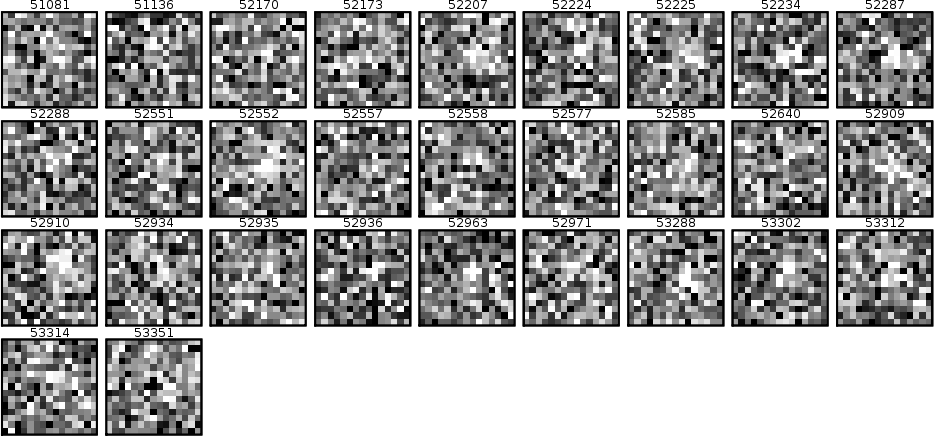
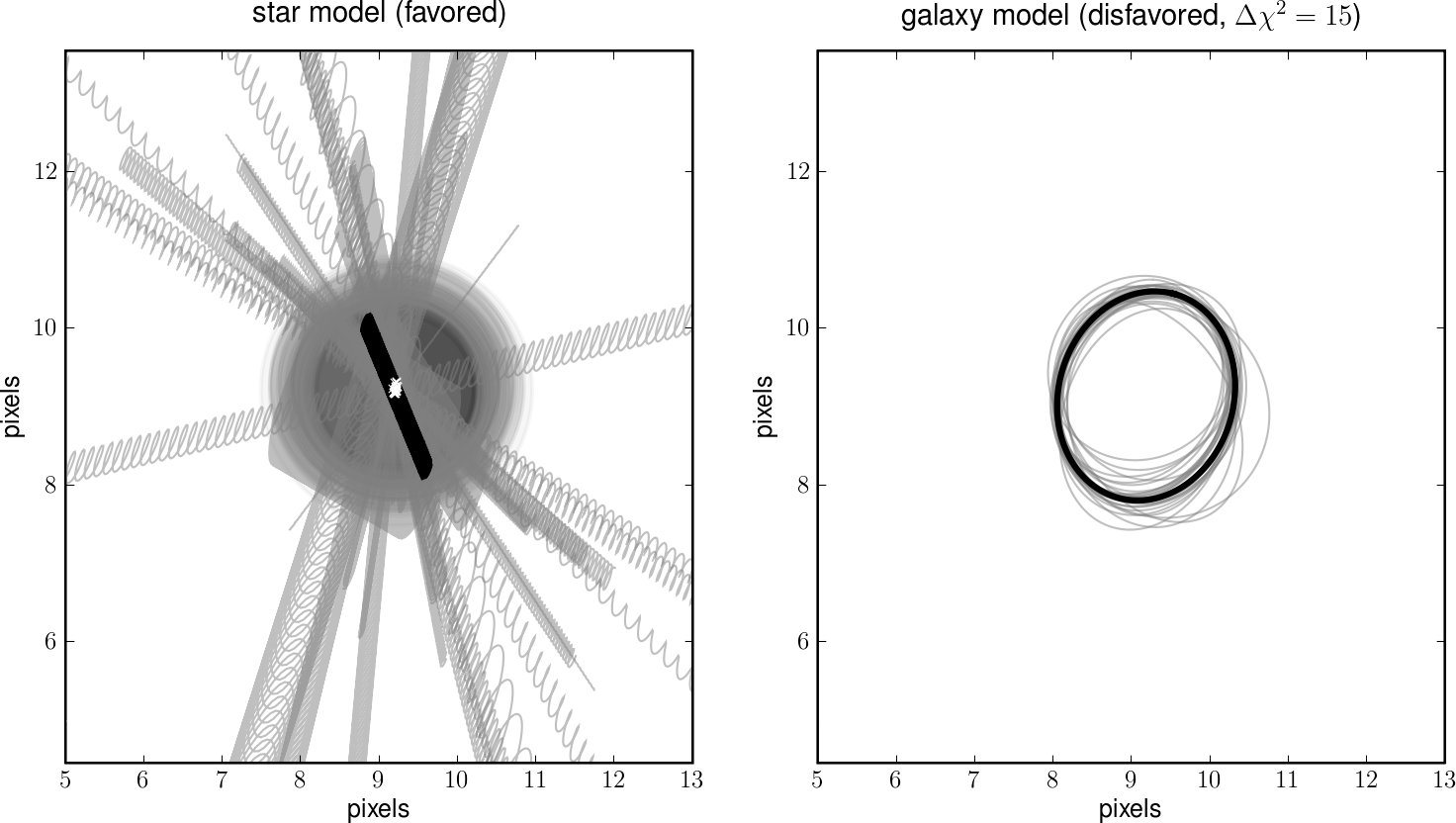
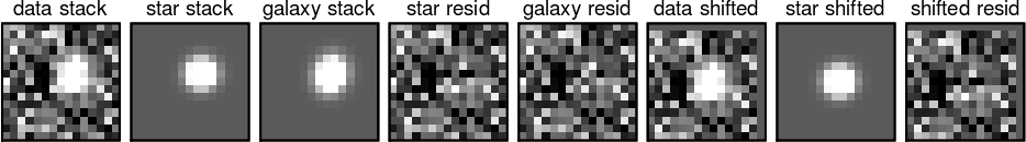
Figure 2: The same as Figure 1 but for SDSS J020332.35+001228.6, a spectroscopically confirmed $z\sim 6$ quasar (Jiang et al., 2008) and $[i-z]>2$ mag source. Here the point-source model is favored, but the inferred proper motion (best-fit value or any sample from the distribution) is very small; the wavy paths each span $\sim 100~{}\mathrm{yr}$ in time; they have different position angles because when the magnitude of the proper motion is constrained to be near zero, the direction is not well constrained. The galaxy model is disfavored by a small amount. The amount is small because the best-fit galaxy model is a non-moving compact source, which is not dissimilar to the nearly non-moving best-fit point source.

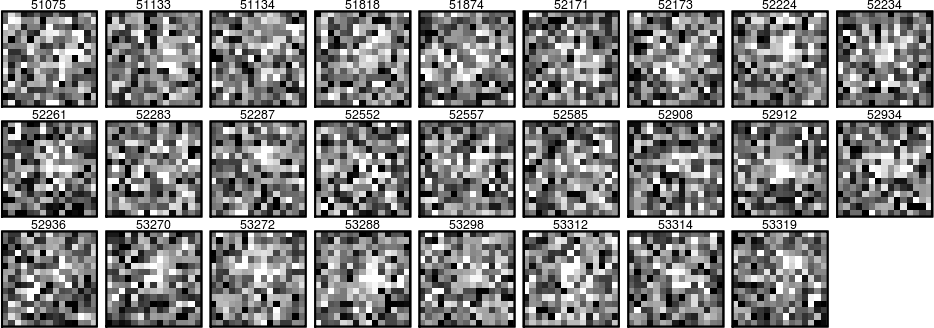
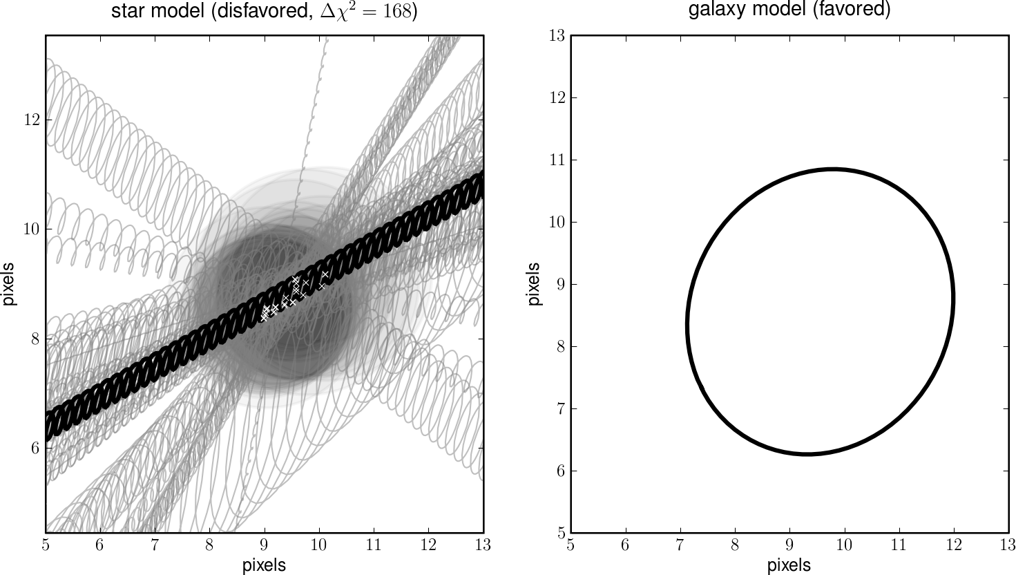
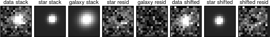
Figure 3: The same as Figure 1 but for a faint galaxy. Here the galaxy model is favored.

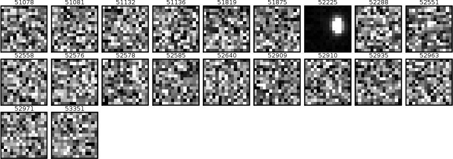
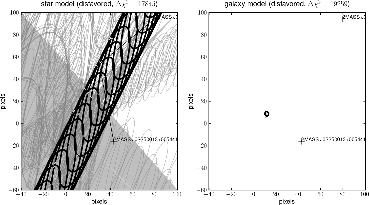
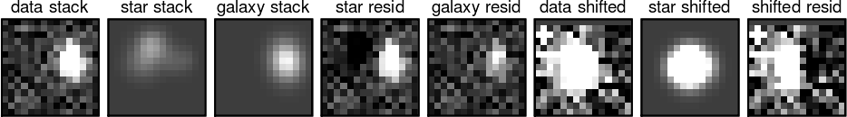
Figure 4: The same as Figure 1 but for a spurious source caused by a blinking artificial satellite. Here the “junk” model is favored over the point-source and galaxy models. Note that the jackknife errors in the point-source and galaxy models are very large. This source actually can be removed by flag-checking in the SDSSSS Coadd Catalog, but we show it here for illustrative purposes.

References

- Adelman-McCarthy et al. (2008) Adelman-McCarthy, J. K., et al. 2008, ApJS, 175, 297
- Abazajian et al. (2009) Abazajian, K., et al. 2009, ApJS(submitted); arxiv 0812.0649v1
- Barron et al. (2008) Barron, J. T., Stumm, C., Hogg, D. W., Lang, D., & Roweis, S., 2008, AJ, 135, 414
- Bernstein et al. (2004) Bernstein, G. M., Trilling, D. E., Allen, R. L., Brown, M. E., Holman, M., & Malhotra, R., 2004, AJ, 128, 1364
- Berriman et al. (2003) Berriman, B., Kirkpatrick, D., Hanisch, R., Szalay, A., & Williams, R. 2003, Large Telescopes and Virtual Observatory: Visions for the Future, 25th meeting of the IAU, Joint Discussion 8, 17 July 2003, Sydney, Australia
- Bramich et al. (2008) Bramich, D. M., et al., 2008, MNRAS, 386, 887
- Casali et al. (2007) Casali, M., et al., 2007, A&A, 467, 777
- Chiu et al. (2008) Chiu, K., et al., 2008, MNRAS, 385, L53
- Dehnen & Binney (1998) Dehnen, W., & Binney, J. J. 1998, MNRAS, 298, 387
- Fan et al. (2000) Fan, X., et al., 2000, AJ, 119, 928
- Fan et al. (2001) Fan, X., et al., 2001, AJ, 122, 2833
- Fuentes et al. (2008) Fuentes, C. I., George, M. R. & Holman, M. J., 2008, arXiv 0809.4166
- Geballe et al. (2002) Geballe, T. R., et al., 2002, ApJ, 564, 466
- Gunn et al. (1998) Gunn, J. E. et al., 1998, AJ, 116, 3040
- Hambly et al. (2008) Hambly, N. C., et al., 2008, MNRAS, 384, 637
- Hawley et al. (2002) Hawley, S. L., et al., 2002, AJ, 123, 3409
- Hewett et al. (2006) Hewett, P. C., Warren, S. J., Leggett, S. K., & Hodgkin, S. T., 2006, MNRAS, 367, 454
- Hogg et al. (2005) Hogg, D. W., Blanton, M. R., Roweis, S. T., & Johnston, K. V., 2005, ApJ, 629, 268
- Irwin et al. (2008) Irwin, M., et al., 2008, in preparation
- Jiang et al. (2008) Jiang, L., et al., 2008, AJ, 135, 1057
- King (1983) King, I. R., 1983, PASP95, 163
- Knapp et al. (2004) Knapp, G. R., et al., 2004, AJ, 127, 3553
- Lawrence et al. (2007) Lawrence, A., et al., 2007, MNRAS, 379, 1599
- Lépine et al. (2003) Lépine, S., Rich, R. M., & Shara, M. M., 2003, AJ, 125, 1598
- Levenberg (1944) Levenberg, K., 1944, The Quarterly of Applied Mathematics, 2, 164
- Lourakis (2004) Lourakis, M. I. A., 2004, http://www.ics.forth.gr/lourakis/levmar
- Lupton et al. (1999) Lupton, R. H., Gunn, J. E. & Szalay, A. S., 1999, AJ, 118, 1406
- Lupton et al. (2001) Lupton, R., Gunn, J. E., Ivezic, Z., Knapp, G. R., Kent, S. M., & Yasuda, N., 2001, ASPC, 238, 269
- Marquardt (1963) Marquardt, D., 1963, SIAM Journal on Applied Mathematics, 11, 431
- Metchev et al. (2008) Metchev, S. A., Kirkpatrick, J. D., Berriman, G. B., & Looper, D., 2008, ApJ, 676, 1281
- Padmanabhan et al. (2008) Padmanabhan, N., et al., 2008, ApJ, 674, 1217
- Pier et al. (2003) Pier, J. R., Munn, J. A., Hindsley, R. B., Hennessy, G. S., Kent, S. M., Lupton, R. H., & Ivezic, Z., 2003, AJ, 125, 1559
- Skrutskie et al. (2006) Skrutskie, M. F., et al., 2006, AJ, 131, 1163
- Smith et al. (2002) Smith, J. A. et al., 2002, AJ, 123, 2121
- Tse (2008) Tse, A., 2008, http://projects.liquidx.net/python/browser/pylevmar
- Vrba et al. (2004) Vrba, F. J. et al., 2004, AJ, 127, 2948
- York et al. (2000) York, D. G. et al., 2000, AJ, 120, 1579