Numerical Relativity Simulations of Precessing Binary Neutron Star Mergers

Abstract

We present the first set of numerical relativity simulations of binary neutron mergers that include spin precession effects and are evolved with multiple resolutions. Our simulations employ consistent initial data in general relativity with different spin configurations and dimensionless spin magnitudes $\sim 0.1$. They start at a gravitational-wave frequency of $\sim 392$ Hz and cover more than $1$ precession period and about 15 orbits up to merger. We discuss the spin precession dynamics by analyzing coordinate trajectories, quasi-local spin measurements, and energetics, by comparing spin aligned, antialigned, and irrotational configurations. Gravitational waveforms from different spin configuration are compared by calculating the mismatch between pairs of waveforms in the late inspiral. We find that precession effects are not distinguishable from nonprecessing configurations with aligned spins for approximately face-on binaries, while the latter are distinguishable from a nonspinning configurations. Spin precession effects are instead clearly visible for approximately edge-on binaries.

For the parameters considered here, precession does not significantly affect the characteristic postmerger gravitational-wave frequencies nor the mass ejection. Our results pave the way for the modeling of spin precession effects in the gravitational waveform from binary neutron star events.

I Introduction

The recent observation of gravitational waves (GW) and electromagnetic (EM) signals from the merger of two neutron stars (NSs) marks a breakthrough in the field of multi-messenger astronomy Abbott et al. (2017); GBM (2017). In order to interpret the detected GW and EM signals accurate models for the coalescence of compact binaries are required. Because of the complexity of Einstein’s field equations coupled to the equations governing general relativistic hydrodynamics those models are based on or compared to numerical relativity (NR) simulations.

To be prepared for future GW detections of unknown binary neutron star (BNS) systems, one needs to cover the entire parameter space, including a variety of Equations of State (EOSs), different mass ratios, and NS spins. While observations of pulsars in BNS systems suggest that most NSs have relatively small spins Kiziltan et al. (2013); Lattimer (2012), this conclusion might be biased by the small number of observed BNSs. Indeed, pulsar observations indicate that NSs in binary systems can have a significant amount of spin. Some stars can even approach the rotational frequency of isolated millisecond pulsars. For example, the NS in the binary system PSR J1807$-$2500B has a rotation frequency of $239$Hz Lorimer (2008); Lattimer (2012). In known double NS systems the fastest spinning pulsar, PSR J0737$-$3039A, has rotational frequency of $44$Hz Burgay et al. (2003). Assuming magnetic dipole and gravitational wave radiation PSR J0737$-$3039A will only spin-down marginally before its merger showing that NSs can have a significant amount of spin when they merge Tichy (2011); Dietrich et al. (2015a).

In addition to the spin magnitude, also the orientation of spins in BNS systems is highly uncertain. Considering BNSs formed in situ, misaligned spins with respect to the orbital angular momentum can be caused by kicks created during the supernova explosions forming the two NSs. While after its formation the primary NS might accrete material from the secondary star, which is at this time in an earlier stage of its evolution and not a NS, this is impossible for the secondary star Chruslinska et al. (2017). Consequently a realignment of the spin caused by accretion is only likely for the more massive NS. Thus, the supernova explosion of the secondary star might introduce a spin kick creating a large misalignement angle. For example PSRJ0737-3039B has a spin misaligned with the orbital angular momentum by $\approx 130^{\circ}$ Farr et al. (2011). For BNS systems formed by dynamical capture, e.g. in globular clusters, there is no reason to assume that spins are aligned to the orbital angular momentum. Overall, further work is needed for a better understanding of the formation scenario of BNS systems and to quantify the imprint of spin on the binary evolution process.

To extract the binary properties, e.g. spin, from a measured GW signal, the detected signal is cross-correlated with template waveforms. The requirements for the template bank is twofold. First, the creation of the waveforms needs to be reasonable fast to allow the computation of a large number of waveforms in a small amount of time. Second, the templates need to capture accurately the binary evolution. For the long inspiral of BNSs detectable by advanced GW interferometers these requirements are challenging.

Considering the recent BNS detection Abbott et al. (2017) a Post-Newtonian (PN) approximant Sathyaprakash and Dhurandhar (1991); Vines et al. (2011) and an approximant incorporating results from the effective-one-body model Bohé et al. (2017) with a phenomenological representation of tidal effects Dietrich et al. (2017a) have been used. Both models describe binaries in which the spins are aligned/anti-aligned with the orbital angular momentum and precession does not occur. Thus, an important scientific target is the development of waveform models for BNS that include precession.

Also in NR simulations spin and precession effects have not been studied in great detail. For a long time spins have been neglected (irrotational binaries) or have been treated unrealistically by assuming that the stars are tidally locked (corotational configurations). Only in the last few years, NR groups performed spinning NS simulations dropping the corotational assumption. Most simulations of spinning binaries use approximate initial data by employing constraint violating data Kastaun et al. (2013); Tsatsin and Marronetti (2013); Kastaun and Galeazzi (2015); Kastaun et al. (2017) or by employing constraint satisfying data which, however, do not fulfill the equations for hydrodynamical equilibrium East et al. (2016a); Paschalidis et al. (2015); East et al. (2016b). Simulations employing constraint solved data fulfilling the equations for hydrodynamical equilibrium have been presented in Bernuzzi et al. (2014); Dietrich et al. (2015a); Tacik et al. (2015); Dietrich et al. (2017b, a). Most of these simulations focused on spin-aligned cases. A precessing NS inspiral has been shown in Tacik et al. (2015) excluding the merger of the stars, and in Ref. Dietrich et al. (2015a) a single precessing simulation at low resolution has been presented. The purpose of this article is to present BNS simulations for two precessing systems for various resolutions and to compare those with spin-aligned configurations.

The article is structured as follows: in Sec. II we give an overview of the studied configurations and the employed numerical methods; in Sec. III accuracy measures for the simulations are presented; in Sec. IV we discuss the dynamics focusing on the precession dynamics and the conservative dynamics in terms of binding energy vs. specific angular momentum plots; in Sec. V and Sec. VI we discuss gravitational waves and the dynamical ejecta. We conclude in Sec. VII.

II BNS Configurations

Table 1: Initial data for the evolutions considered in this work. The columns refer to: the simulation name, the gravitational masses of star A and B, the stars’ dimensionless angular momenta $\chi^{A,B}$ magnitude and their orientation $\hat{\chi}^{A,B}$. All configurations are evolved with the three different resolutions stated in Tab. 2. This makes a total of 15 simulations.

name	$M^{A}$	$M^{B}$	$\chi^{A}$	$\chi^{B}$	$\hat{\chi}^{A}$	$\hat{\chi}^{B}$
SLy(↑↑)	1.3547	1.1067	$0.077$	$0.089$	$(0,\ 0,\ 1)$	$(0,\ 0,\ 1)$
SLy(↗↗)	1.3553	1.1072	$0.13$	$0.16$	$\frac{(1,1,1)}{\sqrt{3}}$	$\frac{(1,1,1)}{\sqrt{3}}$
SLy(00)	1.3544	1.1065	$0.00$	$0.00$	—	—
SLy(↙↙)	1.3553	1.1072	$0.13$	$0.16$	- $\frac{(1,1,1)}{\sqrt{3}}$	- $\frac{(1,1,1)}{\sqrt{3}}$
SLy(↓↓)	1.3547	1.1067	$0.077$	$0.089$	$(0,\ 0,\ -1)$	$(0,\ 0,\ -1)$

II.1 Binaries properties

We study BNSs with two unequal mass NSs with fixed rest masses of $M_{b}^{A}=1.5000M_{\odot}$ and $M_{b}^{B}=1.2000M_{\odot}$. The configurations differ in their spin magnitudes and spin orientation. The NS masses in isolation are $M^{A}\approx 1.35M_{\odot}$ and $M^{B}\approx 1.11M_{\odot}$, leading to a binary mass of $M\approx 2.46M_{\odot}$. Small differences are present because of the different spin magnitudes, see details in Tab. 1.

In Ref. Dietrich et al. (2015a) we have already presented results for one precessing, one spin aligned, and one non-spinning configuration employing low resolutions (resolution R1 in Tab. 2). Here we include also a simulation for an antialigned spin, and an additional precessing configuration. Furthermore, we evolve all systems for three resolutions, which allows us to include error estimates. Details about the initial configurations can be found in Tab. 1 and are summarized in the following.

SLy^(↗↗) is the precessing system considered in Dietrich et al. (2015a), where the two spins of the NSs are pointing along the room diagonal, SLy^(↑↑) has the same spin magnitude parallel to the orbital angular momentum, which ensures for $t=0$ the same spin-orbit contribution as for SLy^(↗↗). However, this leads to a spin magnitude $\sqrt{3}$ times smaller than for SLy^(↗↗). The corresponding non-spinning simulation is denoted by SLy⁽⁰⁰⁾. Additionally, we consider SLy^(↙↙) for which the spins are pointing in the opposite direction as for SLy^(↗↗) and a configuration with spins opposite to SLy^(↓↓). This ensures initially the same spin-orbit coupling for SLy^(↙↙) and SLy^(↓↓).

Table 2: Grid configurations for our simulations. The columns refer to: $L$ total number of levels, $n$ number of points per direction, $L_{\rm mv}$ number of moving box levels using $n_{\rm mv}$ points per direction, $h_{0}$ coarsest grid spacing, and $h_{L}$ finest grid spacing.

Name	$L$	$n$	$L_{\rm mv}$	$n_{\rm mv}$	$h_{0}$	$h_{L}$
R1	7	160	4	64	15.68	0.245
R2	7	240	4	96	11.76	0.184
R3	7	320	4	128	7.84	0.123

II.2 Numerical methods

The initial data for our numerical simulations are computed with the pseudo-spectral code SGRID Tichy (2009) allowing to construct spinning NSs with arbitrary spin and different EOSs Tichy (2012); Dietrich et al. (2015a). Although SGRID allows the construction of eccentricity reduced intial data, we do not perform any kind of eccentricity reduction to save computational costs. However, the residual eccentricities in our simulations are small and stay below $\lesssim 10^{-2}$. We use the same resolution as in our previous works, namely $n_{A}=n_{B}=n_{\rm cart}+4=28$ points, see Tichy (2012); Dietrich et al. (2015a) for a detailed description.

The dynamical simulations are performed with the finite differencing code BAM Brügmann et al. (2008); Thierfelder et al. (2011); Dietrich et al. (2015b); Bernuzzi and Dietrich (2016). The numerical method is based on the method-of-lines, Cartesian grids and finite differencing. The grid is made out of a hierarchy of cell-centered nested Cartesian boxes consisting of $L$ refinement levels, which we label with $l=0,...,L-1$ ordered by increasing resolution. The resolution inside each level increases by a factor of $2$ and can be computed according to $h_{l}=2^{-l}h_{0}$. For completeness we give $h_{L}$ and $h_{0}$ in Tab. 2. The inner levels employ $n_{\rm mv}$ points per direction and move following the technique of ‘moving-boxes’, while the outer levels remain fixed and employ $n$ grid points per direction. We use a Runge-Kutta type integrator for the time evolution. For the time stepping the Berger-Collela scheme is employed enforcing mass conservation across refinement boundaries Berger and Oliger (1984); Dietrich et al. (2015b). Metric spatial derivatives are approximated by fourth order finite differences. The general relativistic hydrodynamic equations are solved with standard high-resolution–shock-capturing schemes based on primitive reconstruction and the local Lax-Friedrich central scheme for the numerical fluxes, see Thierfelder et al. (2011); Bernuzzi et al. (2012a).

Simulating spin precession does not allow us to impose any grid symmetry. This is the major difference to most of our previous simulations, in which we imposed bitant symmetry, and results in double computational cost per configuration. In order to compare the precessing runs to the non-spinning or spin-aligned ones, we choose not to impose any symmetry also for the non-precessing configurations. The grid configurations are given explicitly in Tab. 2, we use three different resolutions for all setups denoted by R1, R2, R3.

III Simulations’ accuracy

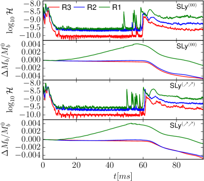
Figure 1: Hamiltonian constraint (first and third panel) and restmass conservation (second and fourth panel) for the non-spinning case SLy⁽⁰⁰⁾ (top) and the precessing case SLy^(↗↗) (bottom).

This section discusses the accuracy of our simulations. Previous detailed studies have been presented in Bernuzzi et al. (2012b); Dietrich et al. (2015b); Bernuzzi and Dietrich (2016); Dietrich et al. (2017c); Dietrich and Hinderer (2017). This work differs from previous ones mainly because no symmetry assumption for the computational grid has been made. Note also that our current best production runs employ high-order finite differencing operators for hydrodynamics Bernuzzi and Dietrich (2016), while here we employed a robust but second-order scheme for the numerical flux. [The higher-order algorithm was not available when this project was started.]

III.1 Constraint violation and mass conservation

In order to assess the validity of our simulations we present the $L_{2}$ volume norm of the Hamiltonian constraint and the conservation of rest mass in Fig. 1 for the precessing case SLy^(↗↗) (top panels) and for the non-spinning case SLy⁽⁰⁰⁾ (botton panels).

Due to the constraint propagation and damping properties of the Z4c evolution system the constraint stays at or below the value of the initial data. The main origin of the wiggles during the orbital motion is the mesh refinement following the motion of the NSs and reflections from the interface between the shells and Cartesian boxes. At merger the constraint grows by about one order of magnitude due to regridding and to the development of large gradients in the solution, but it remains below the initial level. Subsequently, the violation is again propoagated away and damped. Throughout the simulation we find that the Hamiltonian constraint violation improves monotonically with increasing resolution.

The violation of the rest-mass conservation happens at mesh refinement boundaries and due to the artificial atmosphere treatment, and possibly mass leaving the computational domain. Considering the time evolution of the mass violation, we find that, independent of the spin, the resolution R1 shows an increasing mass during the orbital motion. That is caused by insufficient resolution and the artificial atmosphere treatment. For resolutions R2 and R3 the rest mass stays constant within $0.005\%$ during the inspiral. After the merger the rest mass is decreasing. The mass loss is caused by the ejected material which decompresses while it leaves the central region of the numerical domain. Once the density drops by $9$ orders of magnitude, the material is counted as atmosphere and not further evolved. Consequently, conservation of total mass is violated. Overall the mass violation is below $0.4\%$.

III.2 Waveform accuracy

In Fig. 2 we present the GW phase difference between different resolutions for SLy⁽⁰⁰⁾ (top panels) and SLy^(↗↗) (bottom panels) during the inspiral up to the moment of merger, which we define as the time of maximum amplitude in the (2,2)-mode. Through most of the inspiral we see a monotonic decrease of the phase difference for increasing resolution, however, a few orbits before merger the phase difference has a zero and grows again. Such zero crossings are caused by competing effects influencing the overall phase evolution, in particular, the high numerical viscosity for small resolutions and the violation of mass conservation. These zero-crossings have been observed also in other numerical simulations Bernuzzi and Dietrich (2016); Kiuchi et al. (2017). In Bernuzzi and Dietrich (2016) and Dietrich et al. (2017a) we found that employing high-order schemes leads to a constant convergence order for the GW phase for multiple EOSs and grid setups. A similar convergence order can be achieved also for precessing binaries if high-order schemes are employed Radice et al. (2014); Bernuzzi and Dietrich (2016). While not yet in convergent regime, our results are consistent and improve with the grid resolution.

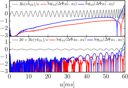
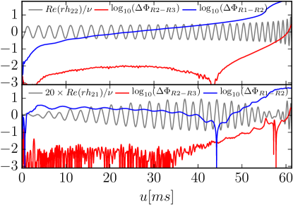
Figure 2: Real part of the (2,2) and (2,1) mode for resolution R3 as well as the phase difference between different resolutions for the SLy⁽⁰⁰⁾ (top) and SLy^(↗↗) (bottom) configurations shown versus retarded time. We multiply the amplitude of the (2,1) mode by a factor of $20$ for better visibility.

IV Dynamics

IV.1 Precession Dynamics

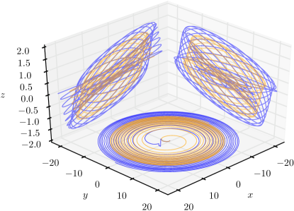
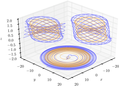
Figure 3: Projection of the NS trajectories of SLy^(↗↗) (top panel) and SLy^(↙↙) (bottom panel) onto the $x$-$y$, $x$-$z$, $y$-$z$-plane. Initially the orbital plane and the $x$-$y$ plane coincide. The trajectory of the more massive star $A$ is shown orange and the trajectory of its companion (star $B$) is drawn blue.

All systems start at an initial GW frequency of $M\omega_{22}=0.030$, which corresponds to a frequency of $392$Hz. This leads to about $\sim 15$ orbits before the NSs merge for the non-spinning case, where the exact number depends on the spin magnitude and orientation. In Fig. 3 we present the trajectories of the NSs for SLy^(↗↗) (top panel) and SLy^(↙↙) (bottom panel). Initially the two stars are located at ${\bf r}_{A}=(-17.2,0.0,0.0)$ and ${\bf r}_{B}=(21.0,0.0,0.0)$. They start to leave the $x$-$y$-plane during the simulation due to the misaligned spin Kidder (1995); Apostolatos et al. (1994). The maximum angle between the $x$-$y$-plane and the orbital plane can be roughly estimated as $\alpha\approx z(t^{*})/\sqrt{x^{2}(t^{*})+y^{2}(t^{*})}$, where $t^{*}$ is chosen in a way such that $z$ is maximal. We find $\alpha\approx 0.11\approx 6^{\circ}$.

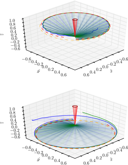
Figure 4: Evolution of the orientation of the angular momentum (solid red curve), the spin of the primary NS (solid green curve) and the secondary star (solid blue curve) for SLy^(↗↗) (top panel) and SLy^(↙↙) (bottom panel). The individual spin of the stars is estimated according to Eq. (1) on coordinate spheres with $r_{s}=14$. We also include PN estimates obtained with the code of Boyle (2013) using the NR data extracted about $1{\rm ms}$ after the start of the simulation as initial conditions, where the precession cone of the orbital angular momentum is shown as a think black line, of the spin of the primary star as a dashed red line and of the secondary star as a orange dashed line.

We further access the precession dynamics by computing the precession cones, cf. Fig. 4. The figure shows the precession cones for the orbital angular momentum (red), the spin of star A (green), and the spin of star B (blue) for the configurations SLy^(↗↗) (top) and SLy^(↙↙) (bottom). The precession cones for the individual stars are based on the quasi-local spin measurement introduced in Dietrich et al. (2017b)

$$S^{i}\approx\frac{1}{8\pi}\int_{r_{s}}\text{d}^{2}x\sqrt{\gamma}\left(\gamma^{kj}K_{lk}-\delta_{l}^{j}K\right)n_{j}\varphi^{li},$$ (1)

evaluated on coordinate spheres with radius $r_{s}$ around the NSs. $\varphi^{li}=\epsilon^{lik}x_{k}$ defines the approximate rotational Killing vectors in Cartesian coordinates ($\varphi^{l1},\varphi^{l2},\varphi^{l3}$), $K_{ij}$ denotes the extrinsic curvature, $\gamma^{ij}$ is the inverse 3-metric, and $n_{i}=(x_{i}-x_{i}^{\rm NS})/r$ is the normal vector with respect to the center of the NS, see also Tacik et al. (2015); Kastaun et al. (2017). The precession cone considering the orbital angular momentum is computed from the stars’ trajectories, where we use $\bm{\hat{L}}=\bm{\hat{r}}\times\text{d}\bm{\hat{r}}/\text{d}t$, with $\bm{r}$ being the vector connecting star A and B.

From Fig. 4 one can see that both configurations SLy^(↙↙) and SLy^(↗↗) contain more than one full precession cycle. In addition to precession, the system also undergoes nutation, i.e. small oscillations occurring at about twice the orbital frequency and thus on a timescale much shorter than the precession timescale. These nutation cycles are visible for the individual spins for SLy^(↗↗), but are also present for SLy^(↙↙). Caused by the particular definition of the spin axis nutation effects in NR simulations differ from those in PN theory Owen et al. (2017).

We compare the numerical relativity results with PN predictions, obtained from the TaylorT4 approximant as implemented in GWframes Boyle (2013). To allow a direct comparison we use as initial conditions the spin and frequency estimated about $1{\rm ms}$ after the beginning of the simulation. We find agreement between the NR results and the PN predictions regarding the overall spin precession. However, during the late inspiral the PN and NR data start to disagree. We surmise that the differences are caused by (i) the fact that the PN prediction looses its accuracy close to the merger; (ii) that possible tidal effects start to effect the evolution; (iii) that the quasi-local spin measure has a decreasing accuracy once the two stars approach each other.

Let us further focus on the evolution of the orbital angular momentum (red) and total angular momentum (black) for the precessing systems, see Fig. 5. While the orbital angular momentum is estimated as before from the tracks of the individual stars, we use for the total angular momentum the ADM-angular momentum of the simulated spacetime. From the figure we can conclude that: (i) The total angular momentum (black), estimated from the ADM angular momentum $J_{\rm ADM}$ does not coincide with the $z$-direction of the numerical grid due to the intrinsic spin of the NSs. (ii) The total angular momentum (black) is not constant due to the emission of GWs (see inset in Fig. 5). (iii) In addition to the precession of the orbital angular momentum, nutation is visible in the orbital angular momentum. Precession and nutation are expected to occur in such systems because the total angular momentum vector is not aligned with any of the principal axes of the moment of inertia tensor of the system.

In Fig. 5 we also present a consistency check based on the symmetry of SLy^(↙↙) and SLy^(↗↗). The green dashed lines show for each of the two configurations the precession cone obtained by flipping $(\hat{L}_{x},\hat{L}_{y},\hat{L}_{z})\rightarrow(-\hat{L}_{x},-\hat{L}_{y},\hat{L}_{z})$ the angular momentum of the other configuration (SLy^(↙↙) in the top and SLy^(↗↗) in the bottom panel). Under this transformation the precession cones for SLy^(↙↙) and SLy^(↗↗) agree very well, if the sign of the $x$- and $y$-components is flipped. Note that this consistency check only works if the spins of the neutron stars are considerably smaller than the orbital angular momentum, since it requires $L_{z}\gg S_{z}$, since otherwise also an adjustment of $\hat{L}_{z}$ needs to be taken into account.

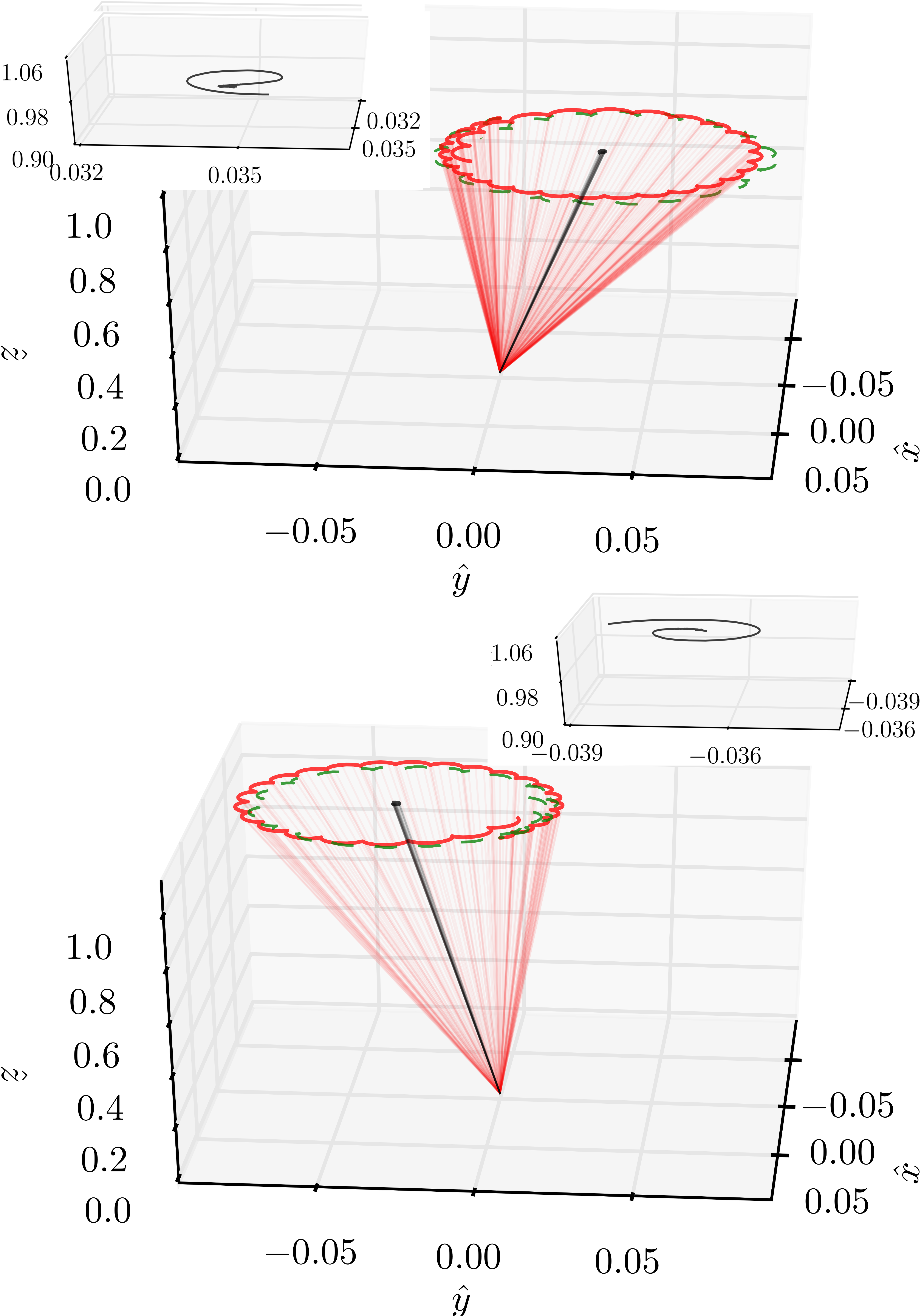
Figure 5: Precession cone for SLy^(↗↗) (top) and SLy^(↙↙) configurations (bottom) for the orbital angular momentum (red). Additionally we present the precession cone of the total angular momentum black, see insets above the main panels. As green dashed line we show the precession cones for $(-\hat{L}_{x},-\hat{L}_{y},\hat{L}_{z})$ for SLy^(↙↙) in the top and SLy^(↗↗) in the bottom panel.

IV.2 Binding energy curves

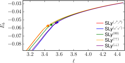
Figure 6: Binding energy $E_{b}$ as a function of the specific orbital angular momentum $\ell$ for all configurations considered in the article. Circles represent the moments of merger.

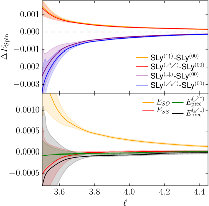
Figure 7: Top panel: Estimate of the spin effects on the conservative dynamics by taking the difference between cases including spin and the irrotational configuration. The shaded region marks the difference to results obtained with a lower resolution and takes into account the uncertainty of the initial data. Bottom panel: Contributions to the binding energy estimated following the discussion given in the text.

In addition to the qualitative discussion presented above, we also investigate the conservative dynamics constructing the binding energy

$$E_{b}=\frac{M_{\rm ADM}(t_{0})-E_{\rm rad}-M}{\nu\ M},$$ (2)

and the reduced orbital angular momentum

$$\ell=\frac{|{\bf{J}_{\rm ADM}}(t_{0})-{\bf{S}_{1}}(t_{0})-{\bf{S}_{2}}(t_{0})-\bf{J}_{\rm rad}|}{\nu\ M^{2}}.$$ (3)

Where $\nu=M^{A}M^{B}/M$ is the symmetric mass ratio, $E_{\rm rad},\bf{J}_{\rm rad}$ are the emitted energy and angular momentum due to GWs, and $M_{\rm ADM},J_{\rm ADM}$ denote the ADM-mass and angular momentum at the beginning of the simulation ($t=t_{0}$), see e.g. Damour et al. (2012); Bernuzzi et al. (2014). ${\bf{S}_{1}}(t_{0})$ and ${\bf{S}_{2}}(t_{0})$ are estimated from the initial data, Tab. 1, and ${\bf{S}}_{A,B}=M^{A,B}\chi^{A,B}\hat{\chi}^{A,B}$.

Figure 6 shows the $E$-$\ell$ curve for all configurations employing the highest resolution R3. During the inspiral (large $\ell$ and $E$) the curves are almost indistinguishable. When the stars approach each other due to the emission of energy and angular momentum, we see clear differences between configurations with aligned spin, without spin, and with anti-aligned spin. This becomes even more prominent in the top panel of Fig. 7 in which we show the difference between all spinning cases with respect to the non-spinning configuration SLy⁽⁰⁰⁾. The shaded region represents our error estimate, which we obtain from assigning to every configuration an error due to the finite resolution estimated by taking the difference between resolution R2 and R3 and by adding an additional uncertainty of $10^{-5}$ to account for the uncertainty of the initial data solver Dietrich et al. (2015a). The final error of the linear combination is obtained from error propagation assuming errors of different configurations are uncorrelated. Note that in case one estimates the error directly from the linear combinations obtained for different configurations, the error reduces by about a factor of $3$, thus we suggest that the error estimates shown in Fig. 7 are conservative estimates.

Assuming that the total binding energy consists of a non-spinning contribution including tidal effects $E_{0}$, a spin-orbit contribution $E_{SO}$, and a spin-spin contribution $E_{\rm SS}$, we can write

$$E_{b}=E_{0}+E_{SO}+E_{SS}+\mathcal{O}(S^{3}),$$ (4)

see also Bernuzzi et al. (2014); Dietrich et al. (2017b).

The bottom panel of Fig. 7 shows the different contributions to the binding energy. The spin-orbit term is estimated according to

$$E_{SO}=\frac{E_{b}[{\rm SLy}^{(\uparrow\uparrow)}]-E_{b}[{\rm SLy}^{(\downarrow\downarrow)}]}{2}$$ (5)

and in general is at leading order proportional to $(\propto\bm{L}\cdot\bm{S}_{i}/r^{3})$, see Kidder et al. (1993). The spin-spin term consists of a self-spin term and an interaction term between the two spins. The interaction term is given by $E_{SS}\propto[3(\bm{n}\cdot\bm{S_{1}})(\bm{n}\cdot\bm{S}_{2})-(\bm{S}_{1}\cdot\bm{S}_{2})]/r^{3}$, see e.g. Kidder et al. (1993). For the precessing systems the spin-spin contribution at the beginning of the simulation is equal to zero due to the particular choice of the spin orientation. We approximate the full spin-spin term (including spin-spin interaction and self-spin) by

$$E_{SS}=\frac{E_{b}[{\rm SLy}^{(\uparrow\uparrow)}]+E_{b}[{\rm SLy}^{(\downarrow\downarrow)}]}{2}-E_{b}[{\rm SLy}^{(00)}].$$ (6)

From Fig. 7 one sees that the spin-spin contribution acts attractive for aligned spin, but is relatively small during most of the inspiral and hardly resolved in our simulations.

To understand the influence of precession, we compute the differences:

$$E_{\rm prec}^{(\nearrow\uparrow)} = E_{b}[{\rm SLy}^{(\nearrow\nearrow)}]-E_{b}[{\rm SLy}^{(\uparrow\uparrow)}],$$ (7)

$$E_{\rm prec}^{(\swarrow\downarrow)} = E_{b}[{\rm SLy}^{(\swarrow\swarrow)}]-E_{b}[{\rm SLy}^{(\uparrow\uparrow)}].$$ (8)

We find overall that $E_{\rm prec}^{(\nearrow\uparrow)}$ and $E_{\rm prec}^{(\swarrow\downarrow)}$ are consistent with zero within our conservative error estimate. Consequently, the conservative dynamics shows only minor differences between precessing systems and systems with the same effective spin but purely aligned/anti-aligned spin. Furthermore, also the spin-spin contribution is within our conservative uncertainty estimate consistent with zero.

V Gravitational Waves

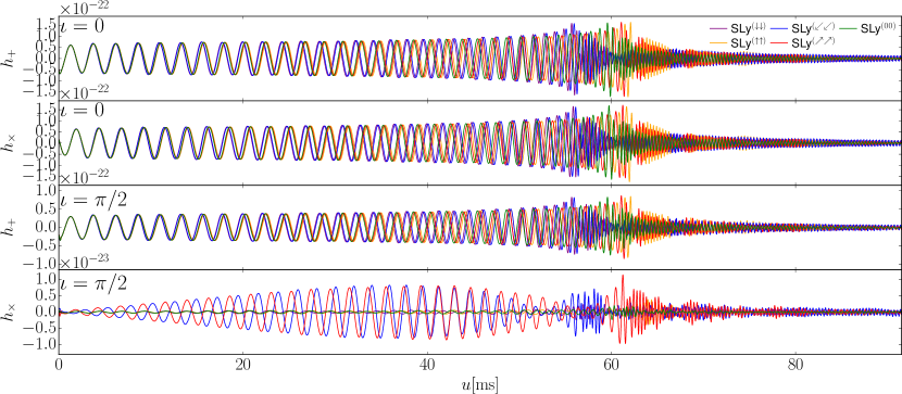
Figure 8: Gravitational wave strains $h_{+}$ (first and third panel) and $h_{\times}$ (second and fourth panel) for the inclinations $\iota=0$ (face on, top panels) and $\iota=\pi/2$ (edge on, bottom panels). We assume a distance to the binary systems of $100{\rm Mpc}$.

V.1 Inspiral Waveform

V.1.1 Qualitative Discussion

We extract GWs from the curvature invariant $\Psi_{4}$ projected on the spin-weighted spherical harmonics for spin $-2$, ${}^{-2}Y_{lm}$, see e.g. Brügmann et al. (2008). Metric multipoles $rh_{\ell m}$ are reconstructed from the curvature multipoles using the frequency domain integration of Reisswig and Pollney (2011). To construct the GW strain $h$ we sum all modes up to $l\leq 4$. All waveforms are shown versus the retarded time computed as

$$u=t-r_{*}=t-r_{\rm extr}-2M\ln\left(r_{\rm extr}/2M-1\right).$$ (9)

In Fig. 8 we present $h_{+}$ and $h_{\times}$,

$$h_{+}-{\rm i}h_{\times}=\sum_{\ell=2}^{4}\sum_{m=-\ell}^{\ell}h_{\ell m}{}^{-2}Y_{\ell m}(\theta=\iota,\phi=0)\ ,$$ (10)

for two inclinations: face on $\iota=0$ (two top panels) and edge on $\iota=\pi/2$ (two bottom panels). According to the plot the following observations can be made:

1. spin-aligned systems merge later, spin anti-aligned systems earlier. This effect, also referred to as orbital hang-up effect Campanelli et al. (2006), is caused by the interaction between spins and the orbital angular momentum Damour (2001).

2. for $\iota=0$ no imprint of precession is visible and cases with the same effective spin evolve similarly.

3. the amplitude of the GWs for $\iota=\pi/2$ is for h₊ about a factor of 2 and for $h_{\times}$ more than an order of magnitude smaller than for $\iota=0$.

4. precession effects with more than one precession cycle are visible in $h_{\times}$ for $\iota=\pi/2$. The amplitude of $h_{\times}$ ($\iota=\pi/2$) for the non-precessing systems is significantly smaller than for the precessing systems, but non-zero due to the unequal masses of the two stars.

V.1.2 Mismatch

Table 3: Mismatch between the different configurations for $h_{+}$ (upper triangle of the table) and $h_{\times}$ (lower triangle of the table). We assume two different inclinations $\iota=0$ (top), $\iota=\pi/2$ (bottom). We restrict our analysis to a frequency window of $f\in[450,2048]$ and use the ZERO_DET_high_P noise curve of Sn: for the computation of the mismatch.

$\iota=0$

$h_{+}/h_{\times}$	$(\downarrow\downarrow)$	$(\swarrow\swarrow)$	$(00)$	$(\nearrow\nearrow)$	$(\uparrow\uparrow)$
$(\downarrow\downarrow)$	-	0.0041	0.0633	0.1179	0.1182
$(\swarrow\swarrow)$	0.0032	-	0.0771	0.1209	0.1217
$(00)$	0.0593	0.0361	-	0.0381	0.0416
$(\nearrow\nearrow)$	0.1137	0.1179	0.0361	-	0.0025
$(\uparrow\uparrow)$	0.1138	0.1186	0.0390	0.0007	-

$\iota=\pi/2$

$h_{+}/h_{\times}$	$(\downarrow\downarrow)$	$(\swarrow\swarrow)$	$(00)$	$(\nearrow\nearrow)$	$(\uparrow\uparrow)$
$(\downarrow\downarrow)$	-	0.0043	0.0609	0.1166	0.1174
$(\swarrow\swarrow)$	0.3762	-	0.0735	0.1207	0.1209
$(00)$	0.1484	0.3549	-	0.0434	0.0460
$(\nearrow\nearrow)$	0.3512	0.0592	0.2765	-	0.0067
$(\uparrow\uparrow)$	0.3181	0.3767	0.1377	0.3252	-

To quantify the influence of spin and precession effects we compute the mismatch between all configurations, see Tab. 3. The mismatch is computed from

$$\bar{F}=1-\max_{\phi_{c},t_{c}}\frac{(h_{1}(\phi_{c},t_{c})|h_{2})}{\sqrt{(h_{1}|h_{1}),(h_{2},h_{2})}}$$ (11)

with $\phi_{c},t_{c}$ being arbitrary phase and time shifts. The noise noise-weighted overlap is defined as

$$(h_{1},h_{2})=4\Re\int_{f_{\rm min}}^{f_{\rm max}}\frac{\tilde{h}_{1}(f)\tilde{h}_{2}(f)}{S_{n}(f)}\text{d}f\ .$$ (12)

For the one-sided power spectral density of the detector noise $S_{n}(f)$ we use the ZERO_DET_high_P noise curve Sn: . We restrict our analysis to a frequency window of $f\in[450,2048]{\rm Hz}$. The chosen lower frequency boundary is slightly above the initial GW frequency to avoid imprints of the junk radiation. The upper boundary is chosen to be the same as in the analysis of the recent BNS detection Abbott et al. (2017).

Considering $\iota=0$, we find that the mismatch between spin-aligned configurations and the non-spinning configuration is about $3\times 10^{-2}$. The mismatch for anti-algined systems is about a factor of $2$ larger which is caused by the lower merger frequency of anti-aligned systems. The computed mismatch between precessing systems and spinning systems with the same effective spin is of the order of $10^{-3}$, which shows that for a face-on detection of a BNS hardly any precession effect might be visible from the late inspiral phase, see e.g. Lindblom et al. (2008).

For edge-on configurations ($\iota=\pi/2$) we find for $h_{+}$ similar results as for $h_{+}$ and $h_{\times}$ for face-on configurations. Considering $h_{\times}$, one finds that systems with the same effective spin parameter do result in large mismatches of the order of $\approx 0.3$. Interestingly, the mismatch between SLy^(↙↙) and SLy^(↗↗) is about a factor of $6$ smaller. However, due to the significantly smaller strain of $h_{\times}$ for $\iota=\pi/2$ a detection of such a configuration is unlikely.

Overall, we find that in the late inspiral precession effects for the employed configurations are small and will most likely not be seen in future GW detections with advanced detectors. However, studies of the entire inspiral visible in the LIGO-Virgo band needs to be performed for further clarification. This will require the creation of waveforms hybridized between our NR waveforms and a precessing inspiral model including tidal effects.

V.1.3 Phase Evolution

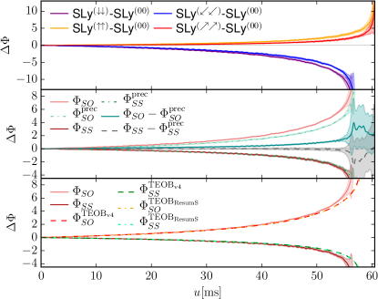
Figure 9: Phase differences. Top panel: Phase differences for all spinning configurations with respect to the non-spinning case. The phase difference is computed with respect to $t=0$. The shaded region is estimated by computing the phase difference for different resolutions. Middle panel: Phase differences between the precessing simulations and the spin aligned/anti-aligned configurations. For all cases we assume an inclination of $\iota=\pi/4$. Bottom panel: Estimate of spin-orbit and spin-spin contribution to the phase from the NR simulations and the EOB approximant TEOBNRv4 Hinderer et al. (2016) and TEOBResumS Bernuzzi et al. (2015a); Damour and Nagar (2014); Nagar et al. (2015) restricted to the (2,2)-mode. Shaded regions correspond to uncertainties assuming error compatible to the difference between different resolutions for the individual configurations.

In the following we want to discuss shortly the phase differences between different configurations. For this purpose we choose an inclination of $\iota=\pi/4$ and discuss phase differences with respect to the beginning of the NR simulations without additional alignment.

Figure 9 shows phase differences for the spinning configurations with respect to the non-spinning configuration (top panel). Visible is an accelerated inspiral due to anti-aligned spin (blue and purple curves) and a decelerated inspiral due to aligned spin (red and orange curves). These phase differences are again caused mainly by the leading order spin-orbit coupling. Notice in addition that all curves show small oscillations which are caused by the fact that an inclination of $\iota=\pi/4$ is chosen. For larger inclinations these oscillations further increase. The opposite holds for smaller inclinations.

To access the influence of different contribution to the phasing , we consider, as for the binding energy, different linear combinations of different numerical simulations, in particular we consider the spin-orbit contribution:

$$\Phi_{SO} = (\Phi[{\rm SLy}^{(\uparrow\uparrow)}]-\Phi[{\rm SLy}^{(\downarrow\downarrow)}])/2,$$ (13)

$$\Phi_{SO}^{\rm prec} = (\Phi[{\rm SLy}^{(\nearrow\nearrow)}]-\Phi[{\rm SLy}^{(\swarrow\swarrow)}])/2,$$ (14)

and spin-spin contribution:

$$\Phi_{SS} = (\Phi[{\rm SLy}^{(\uparrow\uparrow)}]+\Phi[{\rm SLy}^{(\downarrow\downarrow)}])/2-\Phi[{\rm SLy}^{(00)}],$$ (15)

$$\Phi_{SS}^{\rm prec} = (\Phi[{\rm SLy}^{(\nearrow\nearrow)}]+\Phi[{\rm SLy}^{(\swarrow\swarrow)}])/2-\Phi[{\rm SLy}^{(00)}].$$ (16)

The middle panel of Fig. 9 shows our main results. The spin-orbit contribution dominates. Although the precessing configurations and configurations with aligned/anti-aligned are chosen such that the leading order spin-orbit contribution is equal, one sees small differences during the inspiral. The spin-spin effect is significantly smaller than the spin-orbit effect and interestingly is almost identical for the precessing simulations and simulations with aligned/anti-aligned spin. We surmise that the reason for this effect is that, although the spin magnitudes differ, terms proportional to $\propto(\bm{S}_{i}\cdot\bm{L})$ present in the spin-spin contributions are similar.

Finally, as a consistency check, we compare $\Phi_{SO}$ and $\Phi_{SS}$ with results obtained with a spin-aligned tidal effective-one-body (EOB) approximant (bottom panel of Fig. 9). As tidal EOB approximants we use the TEOBNRv4 model of the LIGO Algorithm Library Hinderer et al. (2016) and the TEOBResumS model Nagar et al. . The phases of the tidal EOB approximants are extracted solely from the dominant (2,2)-mode. Both EOB predictions are almost indistinguishable and overall one finds very good agreement between the tidal EOB models and NR results. This shows the accuracy of our numerical simulations and the validity of current state-of-the-art waveform models.

V.2 Postmerger evolution

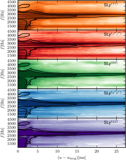
Figure 10: Spectrogram for the all configurations. We shift the beginning of the spectrogram to the merger time (peak in the gravitational wave strain). We include as a black contour the spectrogram of SLy⁽⁰⁰⁾ to all plots. All plots assume an inclination angle of $\iota=\pi/4$.

To access the postmerger GW signal, we compute spectrograms following Dietrich et al. (2017c), see also Bernuzzi et al. (2014); Clark et al. (2015); Rezzolla and Takami (2016). Figure 10 shows the postmerger spectrograms for all configurations under the assumption of $\iota=\pi/4$. We start by discussing the non-spinning configuration SLy⁽⁰⁰⁾ in more detail and later point out differences caused by the intrinsic rotation of the stars.

The middle panel (green) of Fig. 10 shows SLy⁽⁰⁰⁾. Most prominent is the $f_{2}$-peak frequency $f_{2}\approx 2800{\rm Hz}$. One sees that the amplitude of the peak is decreasing while its frequency increases. The frequency increase is caused by the increasing compactness of the star due to the emission of angular momentum in terms of GWs. In addition to the $f_{2}$ peak, additional side peaks and frequencies are visible. Those correspond to the $m=1$ and $m=3$ emission at about $f_{1}\approx 1500{\rm Hz}$ and $f_{3}\approx 4200{\rm Hz}$, respectively. These peaks are harmonic to the $f_{2}$ frequency. As pointed out in e.g. Takami et al. (2014); Bauswein et al. (2014); Rezzolla and Takami (2016) around the moment of merger additional frequency peaks are present, see e.g. the peak at $f\approx 4000{\rm Hz}$.

Considering the difference between SLy⁽⁰⁰⁾ and SLy^(↑↑), SLy^(↗↗), we find that the additional peak around merger at $f\approx 4000{\rm Hz}$ is not present. However, the $f_{1}$ peak is significantly more pronounced during the postmerger evolution for systems with aligned spin. Most importantly, a frequency shift to higher frequencies of about $200{\rm Hz}$ is present. Those shifts are of particular importance in case quasi-universal relations Bauswein et al. (2014); Bauswein and Stergioulas (2015); Takami et al. (2015, 2014); Bernuzzi et al. (2015b) are employed to constrain the NS radius from the postmerger signal Bose et al. (2017); Chatziioannou et al. (2017). Existing relations have been derived for irrotational binaries and might contain systematic biases for spinning systems.

For configurations with anti-aligned spin we find that the additional peaks around merger are visible, see in particular the SLy^(↓↓) configuration. Contrary, the $f_{1}$ peak is less pronounced after the merger. Considering the $f_{2}$-peak frequency, we find that SLy^(↙↙) and SLy^(↓↓) have a similar evolution as SLy⁽⁰⁰⁾.

We do not find noticeable differences between the precessing systems and systems with the same effective spin, but purely aligned or antialigned spin. Thus, we conclude that at least from our simulations we can not impose constraints on precession effects during the inspiral from the postmerger GW signal.

VI Ejecta

Table 4: Ejecta mass and kinetic energy extracted form our simulations given in geometric units.

	SLy(↑↑)	SLy(↗↗)	SLy(00)	SLy(↙↙)	SLy(↓↓)
$M_{\rm ej}$	$5\times 10^{-3}$	$4\times 10^{-3}$	$7\times 10^{-3}$	$7\times 10^{-3}$	$8\times 10^{-3}$
$T_{\rm ej}$	$1\times 10^{-4}$	$6\times 10^{-5}$	$2\times 10^{-4}$	$2\times 10^{-4}$	$2\times 10^{-4}$

In addition to the GW signal emitted from BNS coalescence, possible electromagnetic signals give important information about the binary parameters. To predict the properties of the kilonovae Metzger and Berger (2012); Tanvir et al. (2013); Yang et al. (2015); Metzger (2017); Tanaka (2016) and radio flares Nakar and Piran (2011) one has to know the amount of ejected mass, its geometry, velocity, and composition. In this article we restrict our investigations to dynamical ejected material, which becomes unbound around the time of merger.

In Tab. 4, we give estimates of the masses as well as about the kinetic energy of the ejecta. The uncertainty caused by resolution effects are of the order of $\sim 20\%$, however, larger systematic uncertainties are present due to the artificial atmosphere employed for the evolution Dietrich et al. (2017c). Consequently we want to restrict ourselves to a qualitative discussion.

The mechanisms for dynamical ejecta are either torque in the tidal tail of the stars or shocks created during the merger. In Ref. Dietrich et al. (2017b) was shown that for aligned spin systems torque inside the tidal tail increases. This leads to more massive ejecta in cases in which torque driven ejecta dominate. Here we find that the ejecta mass increases when the NS spin is anti-aligned to the orbital angular momentum. This indicates that the dominant ejecta mechanism are shocks produced during the merger of the two stars, see also Kastaun et al. (2017). A similar trend is observable for the kinetic energy, where overall non-spinning or anti-aligned configurations have ejecta with largest kinetic energy, which will result in larger fluencies of possible radio flares.

We find only a small imprint of precession on the amount of ejected material and differences between precessing systems and systems with the same effective spin are within the uncertainty of our data. Due to the small precession angle of $\approx 6^{\circ}$ of the orbital angular momentum, the ejecta morphology is similar for precessing and non-precessing systems. However, we suggest that for larger spin values or stiffer EOSs precession effects might also be observable. Studying such configurations is left for the future.

VII Conclusion

In this article we studied the effect of spin precession in binary neutron star merger simulations. We considered two precessing configurations, two configurations with aligned/anti-aligned spin, and one non-spinning case. All configurations have been simulated with three different resolutions to assess the uncertainties of our simulations. We find that state-of-the-art numerical relativity simulations are capable to simulate precessing neutron star systems and that spin and precession effects are well resolved.

To interpret the inspiral dynamics, we presented the precession cones of the individual spins and orbital angular momentum. Although the individual spin of NSs in binaries is not defined in general relativity a simple quasi-local spin estimate gives results close to PN predictions.

To quantify the inspiral dynamics we constructed binding energy vs. specific angular momentum curves, finding that precession effects are hardly visible in the conservative dynamics and that the main effect on the binary evolution is, as expected, the spin-orbit interaction.

Considering the effect of precession on the GW signal, we found that for edge-on systems precession effect in the late inspiral are clearly visible. However, those systems are harder to detect due to the smaller observable gravitational wave strain for such inclinations. In contrast for face-on systems precession effects seem to be hardly detectable. Similarly, while the postmerger waveform shows a clear imprint of spin effects in terms of a shift of the main emission frequency of about $200{\rm Hz}$, no noticeable imprint of precession effects is visible. Similarly, in addition to the gravitational wave emission, possible electromagnetic counterparts, mostly triggered by the ejected material, are also unlikely to show noticeable precession effects for the considered configurations.

Further work is needed to quantify the imprint of precession not only during the last milliseconds of the binary neutron star coalescence, but for the full inspiral visible by current gravitational wave detectors already seconds before the actual merger. Additionally, simulations of other configurations with different EOSs, total masses, and mass ratios employing higher resolution are ongoing to further investigate precession effects in a larger region of the binary neutron star parameter space.