Accuracy of numerical relativity waveforms from binary neutron star mergers and their comparison with post-Newtonian waveforms

Abstract

We present numerical relativity simulations of nine-orbit equal-mass binary neutron star covering the quasicircular late inspiral and merger. The extracted gravitational waveforms are analyzed for convergence and accuracy. Second order convergence is observed up to contact, i.e. about 3-4 cycles to merger; error estimates can be made up to this point. The uncertainties on the phase and the amplitude are dominated by truncation errors and can be minimized to $0.13$ $rad$ and $\lesssim 1~{}\%$, respectively, by using several simulations and extrapolating in resolution. In the latter case finite-radius extraction uncertainties become a source of error of the same order and have to be taken into account. The waveforms are tested against accuracy standards for data analysis. The uncertainties on the waveforms are such that accuracy standards are generically not met for signal-to-noise ratios relevant for detection, except for some best cases using extrapolation from several runs. A detailed analysis of the errors is thus imperative for the use of numerical relativity waveforms from binary neutron stars in quantitative studies. The waveforms are compared with the post-Newtonian Taylor T4 approximants both for point-particle and including the analytically known tidal corrections. The T4 approximants accumulate significant phase differences of $2$ $rad$ at contact and $4$ $rad$ at merger, underestimating the influence of finite size effects. Tidal signatures in the waveforms are thus important at least during the last six orbits of the merger process.

I Introduction

An exciting possibility to reveal and to study the nature of the neutron star (NS) interior is provided by the detection of gravitational waves (GWs) from binary neutron star (BNS) mergers. The GWs emitted by BNS during the late inspiral and merger are sensitive to finite size effects, and in particular to the tidal interaction between the bodies, thus they are quantitatively dependent on the star parameters and, in turn, on the equation of state (EoS). Ground-based interferometers are sensitive to the last $10$ orbits of a typical equal-mass binary system of mass $\sim 2.8~{}M_{\odot}$, which roughly corresponds to the frequency range $400-1500~{}Hz$. During this phase tidal effects are expected to be significant.

A general relativistic perturbative theory of tidal interactions has been developed in recent years Hinderer (2008); Damour and Nagar (2009); Binnington and Poisson (2009). These results have been incorporated into the post-Newtonian (PN) formalism Hinderer et al. (2010); Vines and Flanagan (2010); Vines et al. (2011), thus permitting the extension of phasing formulas to tidally interacting binaries, as well as into the effective-one-body (EOB) model Damour and Nagar (2010).

An exact and quantitative evaluation of the dynamics and of the waveforms during the merger process requires, however, the solution of the full nonlinear Einstein equations. In particular, numerical relativity (NR) simulations are to date the only tool to tackle the problem (see e.g. Giacomazzo et al. (2011); Baiotti et al. (2011); Hotokezaka et al. (2011); Sekiguchi et al. (2011); Shibata et al. (2011) for recent works in the field and Faber (2009); Duez (2010); Rosswog (2010) for reviews).

Numerical relativity data have been used in combination with PN methods in order to assess the detectability of tidal effects and the accuracy of the parameter estimated from GW measurements Read et al. (2009). A more recent application of NR results concern their use for calibrating the tidal-EOB model Baiotti et al. (2010a); Baiotti et al. (2011). These works highlight the importance of using NR waveforms and analytic results in order to quantitatively evaluate the impact of tidal effects in the waveforms.

An aspect which deserves a more detailed assessment than is currently available in the literature is the accuracy of the NR waveforms. The estimates of error-bars on phase and amplitude of BNS waveforms, as well as their assessment against accuracy standard for detection Miller (2005); Lindblom et al. (2008); Lindblom (2009), is of fundamental importance for any quantitative study. In constrast to binary black holes (BBHs) data, whose quality for data analysis purposes is well documented, see e.g. Hannam et al. (2009); Reisswig et al. (2009a); Hannam et al. (2010a); MacDonald et al. (2011), convergence and uncertainties in BNS simulations are so far poorly investigated. To our knowledge, the only analysis of truncation errors have been performed in Baiotti et al. (2009), and, more exhaustively, in Thierfelder et al. (2011a). Both works found that the waveforms are second order convergent up to merger but they are limited to short runs (three orbits) and do not consider accuracy criteria for detection. In Baiotti et al. (2011) the same initial data as in this work have been evolved, error bars considering finite-extraction effects and truncation errors have been estimated but without performing convergence tests and using only two simulations. In their conclusions the authors stressed the need for a detailed error budget based on convergence measurements. Since the numerical treatment of the matter (hydrodynamics) makes very challenging to obtain accurate waveforms (in comparison with BBHs simulations), a precise and rigorous assessment of their quality is urgent.

In this work we report results about the accuracy of the waveforms extracted from BNS simulations. Focusing on an example configuration, we consider nine-orbit simulations employing different resolutions, and reaching the highest resolutions for production runs used so far. We discuss convergence in detail, compute error-bars of the waveform amplitude and phase, and test them against accuracy standards for detection. The NR waveforms are then contrasted with the post-Newtonian (PN) T4 phasing formula, both for point-particle and including the leading-order and next-to-leading-order tidal corrections analytically known.

The structure of the paper is as follows. In Sec. II we review our methodology. In Sec. III the simulated binary dynamics is presented. In Sec. IV we analyze the waveforms. In particular, convergence is analyzed in Sec. IV.1, the influence of finite-radius extraction is analyzed in Sec. IV.2, and the waveforms are tested against accuracy standards in Sec. IV.4. In Sec. V the numerical waves are compared with the analytic post-Newtonian T4 formula including tidal effects.

Dimensionless units $c$=$G$=$M_{\odot}$=1 are used in this paper, unless otherwise stated.

II Theoretical and numerical setup

In this section we outline the theoretical and numerical frameworks employed in this paper, and we describe the setup of the simulations. More details on the methodology are given in Brügmann et al. (2008); Thierfelder et al. (2011a) and references therein.

The present study relies on evolutions of BNS initial data within 3+1 numerical relativity, using the BSSNOK formulation Nakamura et al. (1987); Shibata and Nakamura (1995); Baumgarte and Shapiro (1999) of Einstein equations coupled with the general relativistic hydrodynamics (GRHD) system Banyuls et al. (1997). The gauge is specified by the 1+log lapse and Gamma-driver-shift Bona et al. (1995); Alcubierre et al. (2003); van Meter et al. (2006a); Gundlach and Martin-Garcia (2006), using the same expressions and parameters of Sec. II of Thierfelder et al. (2011a). In particular the damping parameter for the shift equation is set to $\eta=0.3$. Gravitational waves are extracted from the numerically generated spacetime by using the Newman-Penrose scalar, $\psi^{4}$. The projections onto spin weighted spherical harmonics, i.e. the multipoles of the radiation, are evaluated on extraction sphere of finite coordinate radius $r$. The same conventions of Brügmann et al. (2008) are employed here. The diagnostic quantities discussed in the following are the ADM mass, $M_{\rm ADM}$, the Hamiltonian constraint, $Ham$, and the rest-mass integral, $M_{0}$, Cf. Eq. (31) of Thierfelder et al. (2011a).

The code employed in this work is the BAM code Thierfelder et al. (2011a); Brügmann et al. (2008, 2004); Brügmann (1999), which implements finite differencing methods on Cartesian refined meshes. The evolution algorithm is based on the method of lines and explicit Runge-Kutta methods (third order in this work). A combination of centered and lop-sided standard finite differences in space is used for the metric fields, see Brügmann et al. (2008). In this work fourth order operators are employed, together with sixth order artificial dissipation. The algorithm implemented for the matter is a robust high-resolution-shock-capturing scheme based on a central scheme for the numerical fluxes Del Zanna et al. (2007); Kurganov and Tadmor (2000); Nessyahu and Tadmor (1990); Shu and Osher (1989a, b). Both the time stepping and the spatial refined mesh are shared with the metric system. The interface fluxes are computed by the local Lax-Friedrichs (LLF) central scheme Nessyahu and Tadmor (1990); Kurganov and Tadmor (2000), while reconstruction is performed with the third order convex-essentially-non-oscillatory (CENO) interpolation Liu and Osher (1998); Del Zanna and Bucciantini (2002). Mesh refinement is provided by a hierarchy of cell-centered nested Cartesian grids and Berger-Oliger time stepping. Metric variables are interpolated in space by means of fourth order Lagrangian polynomials and matter conservatives by a fourth order weighted-essentially-non-oscillatory (WENO) scheme Macdonald and Ruuth (2008). Interpolation in Berger-Oliger time stepping is performed at second order. Some of the mesh refinement levels can be dynamically moved and adapted during the time evolution according to the technique of “moving boxes”, e.g. Brügmann et al. (2008).

Initial data are chosen from quasi-equilibrium configurations of irrotational equal-mass binaries in quasicircular orbits Gourgoulhon et al. (2001); Taniguchi and Gourgoulhon (2002). The configuration selected for this work is a binary with ADM mass $M_{\rm ADM}=M=3.00506$, rest-mass $M_{0}=3.250$, and angular momentum $J_{\rm ADM}=9.716$. The initial proper relative separation is $d\simeq 50$ ($\sim 70~{}km$) corresponding to a GWs frequency $f_{0}=0.0019$ ($394~{}Hz$). The compactness of each star in isolation is $0.14$. The EoS for the fluid is the polytropic one, with adiabatic index $\Gamma=2$. The initial configuration is computed with a multidomain spectral code which solves the Einstein constraint equations under the assumption of a conformally flat metric. The code is based on the Lorene library Eric Gourgoulhon, Philippe Grandclément, Jean-Alain Marck, Jérôme Novak and Keisuke Taniguchi and provided by the NR group in LUTH (Meudon). These initial data represent to date the most accurate computation of equilibrium BNSs and they are publicly available on the web. The same initial data were used for the evolutions discussed in Baiotti et al. (2010a); Baiotti et al. (2011).

Table 1: Summary of the grid configurations and of the runs. Columns: name of the configuration, maximum refinement level, minimum moving level, number of points per direction in the moving levels, resolution per direction in the level $l=l_{\rm max}$, number of points per direction in the nonmoving levels, resolution per direction in the level $l=0$, number of processors, maximal memory usage, and average speed in term of the mass of the configuration evolved ($M=2.998~{}M_{\odot}$) including checkpointing and initialization (reference machine: JUROPA cluster).

Name	$l_{\rm max}$	$l^{\rm mv}$	$N_{\rm xyz}^{\rm mv}$	$h_{\rm l_{\rm max}}$	$N_{\rm xyz}$	$h_{0}$	Nproc	Mem (Gb)	Speed (M/hr)
HH2	7	4	100	0.1875	160	24	64	150	6
HH3	7	4	128	0.1466	176	18.75	64	190	4.5
HH4	7	4	140	0.1328	192	17.14	96	240	5
HH5	7	4	150	0.1250	200	16	256	350	12
HH6	7	4	160	0.1172	212	15	256	400	12

Evolutions were performed for the $\Gamma=2$ polytropic EoS, i.e. we consider the fluid isentropic and neglect thermal effects. In Thierfelder et al. (2011a) we have shown that, in agreement with the physical expectation, waveforms computed with both the polytropic EoS and the ideal gas EoS (which includes in a rough way thermal effects) are indistinguishable within the simulation errors, at least up to contact, while significant differences accumulate during merger and the HMNS phase. In this work we are mainly interested in the inspiral phase, hence thermal effects can be neglected; we will consider thermal effects in the present setup in future work.

Gravitational waves were extracted at levels $l=1,2,3$. Several resolutions and a single grid setup were employed. The latter is composed of a fundamental grid level, $l=0$, and seven refinement levels from $l=1$ to $l_{\rm max}=7$; four refinement levels are moving, $l=4,5,6,7$. The only symmetry assumed is reflection symmetry about the $z=0$ plane, i.e. the numerical domain is restricted to $z>0$. The grid configurations, as well as the performances of the runs are reported in Tab. 1. The grid settings are similar to those of other codes, e.g. Baiotti et al. (2010b). The highest resolution employed here for run HH6 is slightly ($3\%$) higher than the maximum resolution used to date on BNS simulations employing mesh-refined-Cartesian-grid-based codes Baiotti et al. (2011). All the runs were performed with Courant-Friedrich-Lewy (CFL) factor of $0.25$. The (self) convergent series are formed by triplets of runs, that in the following will be denoted as HH$\{LMH\}$, where $L,M,H$ correspond to the low, medium, and high resolution employed. Self-convergence tests can be biased by the choice of the resolutions employed. An “optimal” setup would require that (i) the ratios between the low and medium and medium and high resolutions are $h_{L}/h_{M}\simeq h_{M}/h_{H}\simeq 2$; and (ii) the scaling factor is at least of order two, ${\rm SF}=(h_{L}^{r}-h_{M}^{r})/(h_{M}^{r}-h_{H}^{r})\gtrsim 2$, where $r$ is the convergence rate. It is difficult to obtain an optimal convergent series since low resolutions are too inaccurate and differ even in a qualitative way Thierfelder et al. (2011a). Considering the criteria above, the “best” convergent series is HH$\{235\}$ or HH$\{236\}$.

III Overview of the binary dynamics

In this section we summarize the binary dynamics and present some diagnostic of the simulations.

The binary evolves for about nine orbits dynamics before merger, when a hyper-massive-neutron-star (HMNS) is formed. The latter oscillates non linearly in time, loses angular momentum by GW emission increasing its compactness, and, finally, collapses to a black hole surrounded by a disk rapidly accreting.

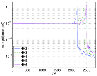
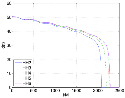
Figure 1: BNS dynamics. (left) Evolution of the maximum of the rest-mass density for different resolutions. (right) Evolution of the proper separation between the two stars.

The evolution of the maximum rest-mass density is reported in Fig. 1 (left), together with the proper distance (right). During the inspiral the maximum of the rest-mass remains constant as expected; the proper distance shows some residual eccentricity from the initial data. The latter is larger during the first three orbits and then progressively radiated away, although not completely. The stars touch each other about $1.5$ orbits before merger ($t/M\gtrsim 2050$), which happen at $t_{\rm m}/M=2259$ for run HH6 (see Sec. IV for the definition of merger used also in this work). After the merger the maximum of the rest-mass density increases indicating the compactness of the HMNS increases; it reaches a peak during the collapse then drops down to the densities of the accretion disk. The quasi-radial oscillations of the HMNS are also visible before the collapse. An apparent horizon is formed at $t_{\rm AH}/M\simeq 2475$ (run HH6), the mass and spin of the final puncture describing the black hole Thierfelder et al. (2011b); Brown (2008); Hannam et al. (2007) are $M_{\rm BH}=2.955\pm 0.005$ and $a_{\rm BH}=0.80\pm 0.01$. The latter values are computed from the irreducible mass and spin, after an initial transient in the BH formation.

Overall the new simulations at higher resolution confirm our previous findings about the merger outcome Thierfelder et al. (2011a): the HMNS experiences a delayed collapse  while a prompt collapse seems an artifact of lower resolution runs (see HH2). Note also that the use of lower resolutions results in earlier mergers.

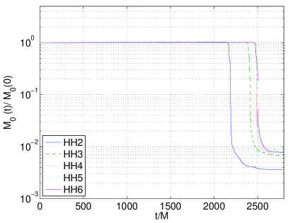
Figure 2: Evolution of the rest-mass density for different resolutions.

The evolution of the rest-mass is reported in Fig. 2. During the inspiral it is conserved up to $\max(\Delta M_{0}/M_{0})\lesssim 1\%$ for runs HH4 and higher resolutions. At the collapse it drops several order of magnitude, similarly to the maximum of rest-mass density. As explained in Thierfelder et al. (2011b) this effect is produced by the gauge conditions which, handling the singularity formation, stretch the numerical grid effectively moving grid points to larger proper radii. The values of $M_{0}$ at late times are an estimate (upper limit) for the rest-mass of the accretion disk, which is below $1\%$ of the initial rest-mass. Note the strong dependence of the result on the resolution.

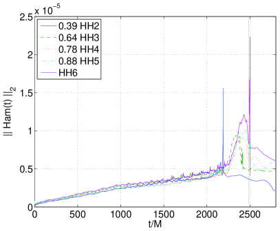
Figure 3: Convergence of the L2 norm of the Hamiltonian constraint. The data set are rescaled for second order convergence to the highest resolution one.

The convergence of the L2 norm of the Hamiltonian constraint is reported in Fig. 3. The different data set are rescaled for second order convergence to the highest resolution one. As one can observe from the figure, the lines are superposed during the inspiral while they progressively differ from the contact, towards the merger. After the merger convergence is not measurable.

Finally we comment about the ADM mass conservation. We computed finite-radius approximations to the ADM mass, $M_{\rm ADM}(r)$, by integrals over coordinate spheres as in the case of the GW, considering two different formulas: (a) Eq. (54) of Brügmann et al. (2008), and (b) the integral of the conformal factor only. The ADM mass is defined for the limit of large spheres, $r\to\infty$. The value at finite $r$ is a coordinate dependent quantity, and, for large but finite $r$, it suffers of resolution problems in the outer levels. In our setup the calculation is not accurate enough to make quantitative statements and extrapolation $r\to\infty$ does not seem to improve the results. We observe anyway a consistency between $M_{\rm ADM}(r)$ and the energy of the emitted GW within the $1~{}\%$ level.

IV Waveforms

The total gravitational energy radiated during the merger process is about $1~{}\%$ of the initial ADM mass. About $99~{}\%$ of the energy radiated during the inspiral is emitted into the $(\ell,m)=(2,2)$ multipolar channel: the latter is also responsible for about the $92~{}\%$ of the energy emitted during the whole simulation. In the following we will consider only the $(2,2)$ mode. Figure 4 (left) shows the real part, the imaginary part, and the absolute value of the GW multipole $r\,h_{22}$ extracted at $r=750$ ($250~{}M$) and from the HH6 run. All the plots relative to the waveforms are in term of the retarded time without changing notation. We use thus $t\to t-r_{*}$, where the tortoise radius is computed as $r_{*}=R+2M\log(R/(2M)-1)$, with $R(r)$ the Schwarzschild radius corresponding to the coordinate extraction (isotropic) radius $r$.

The waveform is characterized by the chirp-like shape typical of the quasi-circular inspirals, after about $18$ cycles it peaks, and then shows a more complicated structure with multiple maxima in amplitude and progressively higher frequencies. We formally define the merger time, $t_{\rm m}$, as the time corresponding to the peak of the amplitude of $r\,h_{22}$ Baiotti et al. (2011); Thierfelder et al. (2011a). The signal after the merger is characterized by the emission from the HMNS. We reported an analysis in Thierfelder et al. (2011a), see also Stergioulas et al. (2011) for recent work. More details will be given in a future work, in the following we will focus on the inspiral waveforms.

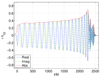
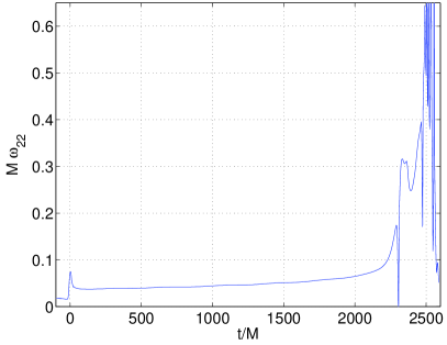
Figure 4: $r\,h_{22}$ waveform. (left) Real part, imaginary part, and amplitude; (right) instantaneous GW frequency. Extraction radius $r=750$, run HH6.

The simulation output is the multipole of the curvature scalar, $\psi^{4}_{22}$. The actual GW strain, $h$, is recovered from $\psi^{4}$ by integrating the relation $\ddot{h}=\psi^{4}$. The integration is not straightforward in the case of noisy numerical data. We employ the method described in Reisswig and Pollney (2010), i.e. we perform the integration in the Fourier frequency domain by applying a fixed-frequency–high-pass filter, following closely Thierfelder et al. (2011a). The cutting frequency used in this work is $f_{\rm cut}=0.0016<f_{0}$. As shown in Fig. 4, the waveform is affected by some amplitude modulations mostly present at early times. Their origin may be due to the residual eccentricity contained in the initial data.

In the following waveforms will be split into phase and amplitude according to the notation,

$$r\,h_{22}=A_{22}\exp{(-i\Phi)}\ ,\ \ \ r\,\psi^{4}_{22}=a_{22}\exp{(-i\phi)}\ .$$ (1)

The instantaneous GW frequency is $\omega=-\Im(\dot{h}/h)$, and is plotted in Fig. 4 (right) in case of the $(2,2)$ multipole. It increases monotonically during the inspiral, and reaches the value $M\,\omega_{22}(t_{\rm m})\simeq 0.123$ at the merger. At $t/M\sim 2400$ it shows a signature of the HMNS, and at later times increases to the quasi normal modes (QNMs) frequencies of the final black hole (BH). Note that the GW frequency drops to zero at $t/M\simeq 2300$, corresponding to a minimum of the amplitude and to a quasi spherical shape of the stars Thierfelder et al. (2011a). The frequency of the BH fundamental QNMs can be extracted from the GW frequency, however a cleaner equivalent signal is provided by the frequency of $r\,\psi^{4}_{22}$. We found for run HH6 $f_{\rm QNM}\simeq 6.47~{}kHz$ ($M\,\omega_{22}\sim 0.6$), in $2~{}\%$ agreement with the estimate obtained from the horizon quantities.

In the following the accuracy of the numerical waveforms is assessed. We stress that here, for the first time, phase and amplitude errors are measured precisely and consistently from convergence tests.

IV.1 Convergence

In this section we present the results concerning the self-convergence of the inspiral waveforms. The convergence series HH$\{236\}$ is discussed as an example, similar results are obtained for HH$\{235\}$. We focus on the extraction radius $r=750$ and on $r\,\psi^{4}_{22}$. Similar results are found for $r\,h_{22}$.

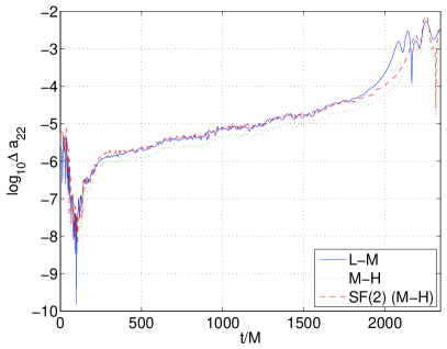
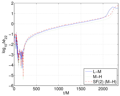
Figure 5: Self-convergence of $r\,\psi^{4}_{22}$ waveforms. The logarithm differences between resolutions in amplitude (left) and phase (right) are shown together with the difference scaled for second order convergence. Extraction radius $r=750$.

In Fig. 5 the self-convergence test is shown. The scaling factor is $SF(2)=1.8$. The differences are noisy so the figure employs a standard Savitzky-Golay averaging filter for a better visualization; results are not affected anyway. The waveforms show compatibility with second order self-convergence during the inspiral up to $t/M\simeq 2000$. At later times they become, as other quantities, progressively over-convergent, and after the merger the convergence order can not be established. We observe here a common finding in NR simulations (e.g. Yamamoto et al. (2008); Baiotti et al. (2009); Thierfelder et al. (2011a)): as long as only the bulk motion of the matter is important, the numerical methods employed do quite well modelling the inspiral due to GW emission, but degrade when strong field and matter dynamics develop.

The over-convergence behavior appearing at late times is probably due to the run HH2, but also to the fact that, when the stars come in contact, the effective order of the (nonlinear) numerical scheme for hydrodynamics probably drops below the second order (in norm). As in previous shorter runs Thierfelder et al. (2011a), the phase is not exactly convergent at rate two but at lower rate (between one and two). Note that, differently from previous works on BNS and consistently with Thierfelder et al. (2011a), we do not align the waveforms for the convergence tests. The gravitational energy carried by the $(2,2)$ mode also shows approximately second order self-convergence.

The interpretation of these data can be delicate because several sources of systematic errors are not completely under control: the exact expected convergence rate, the role of different grid setup, the limited and not optimal choices of resolutions for the convergent series, etc. Our findings, however, appear consistent and sufficiently robust; the second order rate is expected, in convergence regime, by basic arguments, and the diagnostic quantities of Sec. III show second order convergence in norm. The results seem to indicate that second order convergence can be confidently assumed up to contact, or, equivalently, to $M\,\omega_{22}=0.07$. In the following we will assume second order convergence for the extrapolation of the inspiral waveforms up to merger, errors will be given both for $M\,\omega_{22}\leq 0.07$ and for $M\,\omega_{22}\leq 0.1$. The reliability of the latter estimate is not clear.

IV.2 finite-radius extraction

In this section we study the uncertainties on phase and amplitude related to the computation of waveforms at finite-extraction radii. We consider several extraction radii $r=200,\,300,\,400,\,500,\,750$ (or $R\simeq 203,\,303,\,403,\,503,\,753$) from run HH6 and $r\,\psi^{4}_{22}$.

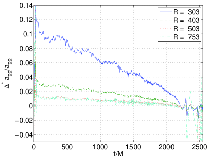
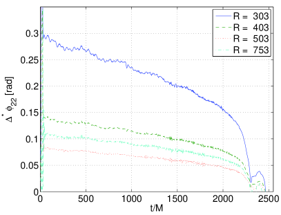
Figure 6: Differences between amplitude (left) and phase (right) of waves extracted at successive radii $r=200,\,300,\,400,\,500,\,750$. Run HH6.

The differences in amplitude and phase extracted at a given radius with the previous, e.g. $\Delta^{*}\phi_{22}(R_{i})=\phi_{22}(R_{i})-\phi_{22}(R_{i-1})$, are shown in Fig. 6. Both amplitude and phase increase for higher extraction radii. The differences are bigger at earlier times, the phase differences at early times scale approximately as $1/r$, while amplitude differences approximately as $1/r^{2}$. For radii $r\geq 400$ differences in amplitude are $\lesssim 2\%$ and they seem to saturate. By contrast differences in phase keep on increasing and between $r=750$ and $r=500$ they are $\sim 0.1$ $rad$. The differences become progressively smaller towards the merger.

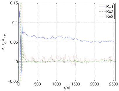
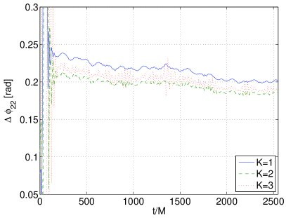
Figure 7: Differences between amplitude (left) and phase (right) of $r\,\psi^{4}_{22}$ extrapolated up to different orders, $K$, and at the reference radius $r=750$. Run HH6.

Following previous works Boyle et al. (2007); Scheel et al. (2009); Boyle et al. (2008); Boyle and Mroue (2009); Pollney et al. (2009, 2011), an approximation of the waves at null-infinity can be obtained by simple $1/R$-extrapolation,

$$F(t,R)=\sum_{k=0}^{K}F_{k}(t)R^{-k}\ ,$$ (2)

where $F(t,R)$ is either the phase or the amplitude, $t$ is the retarded time, and $F_{0}(t)$ is the extrapolated value. In Reisswig et al. (2009b); Reisswig et al. (2010); Babiuc et al. (2011) the robustness of the extrapolation procedure has been assessed against null-infinity waveforms from equal-masses BBH inspirals computed with the Cauchy-characteristic extraction (CCE) method Bishop et al. (1996); Babiuc et al. (2005, 2009). In Bernuzzi et al. (2011a, b), by mean of BH perturbation theory on hyperboloidal foliations, it has been shown that, in case of an unambiguous definition for the background and for the retarded time, the extrapolation reproduce null-infinity waveforms up to their numerical uncertainties for enough high values of $K>3$.

Figure 7 shows the differences between the extrapolated value for different $K$ and the reference radius $r=750$. Note that waveforms at different radii are not shifted in time or phase, but only considered against the retarded time. The fit errors, $\delta F$, are computed at the $68~{}\%$ confidence level, and distributed quite uniformly in the inspiral. Hence, their average, $\left<\delta F\right>$, can be use as a meaningful measure of the fit quality in comparison with the differences, $\Delta F$, between the extrapolated waves and the finite-radius extracted ones. In case of a linear extrapolation, $K=1$, the average fit errors are $\left<\delta\phi_{22}\right>\sim 0.02$ $rad$ and $\left<\delta a_{22}/a_{22}\right>\sim 3~{}\%$, and the maximum differences with the last radius are $\Delta a_{22}/a_{22}\sim+5~{}\%$ and $\max\Delta\phi_{22}\sim+0.23$ $rad$. For $K=2$, the average fit errors are $\left<\delta\phi_{22}\right>\sim 0.04$ $rad$ and $\left<\delta a_{22}/a_{22}\right>\sim 3~{}\%$, and maximum differences with the last radius are $\max\Delta a_{22}/a_{22}\sim+1\%$ and $\max\Delta\phi_{22}\sim+0.21$ $rad$. The use of $K>2$ results in more noisy data as shown by the figure, and also the fit errors increase. The “best” extrapolation is thus given by $K=1$ or $K=2$. Note however that the fit averaged uncertainties are about $10~{}\%$ of the phase difference with the last resolution also in the best cases, and that, within this uncertainty, both the extrapolations basically agree (see right-hand panel of Fig. 7).

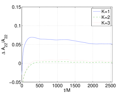
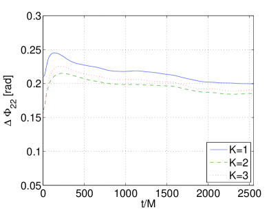
Figure 8: As Fig. 7 but referring to $r\,h_{22}$.

A similar behavior has been observed for the extrapolation of $r\,h_{22}$. In this case however data are less noisy and the fit errors are smaller. Specifically we found $\left<\delta\Phi_{22}\right>\sim 0.006$ $rad$ and $\left<\delta A_{22}/A_{22}\right>\lesssim 2~{}\%$ for $K=1$ and $\left<\delta\Phi\right>_{22}\sim 0.002$ $rad$ and $\left<\delta A_{22}/A_{22}\right>\lesssim 1~{}\%$ for $K=2$. The latter is thus preferable. The differences with the last extraction radius are reported in Fig. 8, and comparable in absolute size to those of Fig. 7.

IV.3 Truncation errors

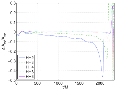
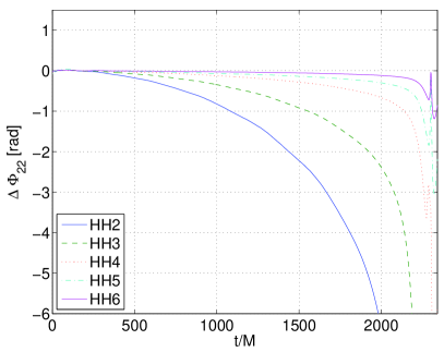
Figure 9: Differences between extrapolated values from series HH$\{23456\}$ and the data at various resolution. Amplitude (left) and phase (right) of $r\,h_{22}$ (bottom). Extraction radius $r=750$.

In this section we quantify the truncation errors in the inspiral waveforms. Richardson extrapolation is employed using different data sets and assuming second order convergence. Extrapolation series are indicated with the same notation of convergence series, e.g. HH$\{23456\}$. Errors are computed as differences with the highest resolution data. We stress that this is a common but optimistic choice. Also, to avoid underestimates of the errors, the whole convergent series is, at least, used in the extrapolation.

Table 2: Maximum differences between extrapolated values in resolution and the highest resolution data (run HH6) in different quantities during the inspiral. The first three rows refer to the maximum errors for $M\,\omega_{22}\leq 0.07$, while the last three rows refer to the maximum errors for $M\,\omega_{22}\leq 0.1$.

Runs	$|\Delta a_{22}/a_{22}|$ [%]	$|\Delta\phi_{22}|$ [$rad$]	$|\Delta A_{22}/A_{22}|$ [%]	$|\Delta\Phi_{22}|$ [$rad$]	$|\Delta\omega_{22}/\omega_{22}|$ [%]
HH$\{236\}$	38	1.8	8	2	9
HH$\{2346\}$	5	0.4	1	0.4	2
HH$\{23456\}$	1	0.13	0.2	0.13	0.6
HH$\{236\}$	$>$100	7	20	5	$>$100
HH$\{2346\}$	70	1.4	6	1.4	15
HH$\{23456\}$	13	0.3	2	0.3	4

Figure 9 shows the differences in amplitude and phase between the extrapolated data from HH$\{23456\}$ and those from run HH6. Similar plots were produced for $r\,\psi^{4}_{22}$ and for different extrapolation series. The differences are negative and increase towards the merger. Before the merger the trend changes and they rapidly increase to positive values. From the argument given at the end of Sec. IV.1, we do not expect to have a fully reliable extrapolation at the merger, thus proper error estimates must be restricted to slightly before that point. In case of other extrapolation series the errors are bigger but qualitatively they show the same behavior. The maximum absolute errors observed before the merger are reported in Tab. 2 for different extrapolation series. They are computed within the GW frequency intervals $M\,\omega_{22}=[0.0358,0.07]$ (i.e. $f\in[f_{0},f_{\rm max}]=[0.0019,0.0037]$), where the extrapolation is reliable, and also within the GW frequency intervals $M\,\omega_{22}=[0.0358,0.1]$. In the latter case they roughly correspond to the minima in Fig. 9.

As shown by the table, it is necessary to include at least four resolutions to obtain a phase error $\Delta\Phi_{22}\lesssim 1$ $rad$ and an amplitude error of $\Delta A_{22}/A_{22}\lesssim 1~{}\%$ for $M\,\omega_{22}\leq 0.07$. In this case truncation errors become of the same order of magnitude of the finite-extraction effect. The error estimate up to $M\,\omega_{22}=0.1$ indicate how dramatically the errors increase up to merger. This analysis suggests that truncation errors represent the main source of uncertainties in BNS simulations.

IV.4 Accuracy

In this section we test the inspiral waveforms against accuracy standards for data analysis. As a measure of the accuracy we employ the square of the inaccuracy functional, $\mathcal{I}^{2}$, whose definition is discussed in detail in Appendix A, Eq. (6). Accuracy requirements are set to minimal levels and an ideal detectors is assumed. As mentioned in Appendix A, two waveforms are distinguishable depending on the signal-to-noise ratio (SNR, $\varrho$) of the detection. Given a difference between two waveforms (the error bars, in our case), $\delta h$, there always exists a sufficiently high SNR such that the difference is significant (in our case, the waveforms are inaccurate). The point is thus to assess the accuracy with respect SNR that are high enough but also realistic for the future detections. We recall that for equal-masses BBH waveforms accuracy standards are achieved for relevant SNR, and waveforms can be considered faithful, e.g. Aylott et al. (2009); Hannam et al. (2009, 2010a); MacDonald et al. (2011). By contrast, such analysis for BNS has never been considered before.

We recall that the inaccuracy functional has been rarely employed in NR literature, see e.g. MacDonald et al. (2011), but it provides an equivalent measure to the most common mismatch functional, $\mathcal{M}$ (see again Appendix A for the definition). The inaccuracy functional is here preferred because its value does not depend on the distance between the detector and the source or on the normalization of the PSD of the detector noise. In the accuracy standards the dependency on the distance from the source is then moved to the right-hand-side of the expressions. All the results presented here can be translated in term of the latter considering that $\mathcal{I}^{2}/\varrho\approx 2\mathcal{M}$ McWilliams et al. (2010); Hannam et al. (2010a).

Table 3: Inaccuracy functional for several configurations. Columns: detector configuration with reference for the noise curve, SNR at $100~{}Mpc$ (assuming the detector and the binary are optimally aligned), inaccuracy functional for different choice of the waveforms. HH$\{2-6\}$ indicates the waveform has been extrapolated in resolution with those runs, ^∗ indicates the extrapolation in radius is performed. The model waveform, $h_{\rm m}$, in the inaccuracy functional is always the one from run HH6 at $r=750$, except for the last column where the extrapolated in radius from the same run is used.

$S_{n}$	$\varrho$	$\mathcal{I}^{2}[h_{\rm m},h_{\rm x}]$
		HH6, HH$\{236\}$	HH6, HH$\{2346\}$	HH6, HH$\{23456\}$	HH6, HH$\{23456\}^{*}$	HH$6^{*}$, HH$\{23456\}^{*}$
advLIGO Ajith and Bose (2009)	3.6	0.333	0.117	0.043	0.149	0.045
advLIGO NSNS Opt LIGO Document T0900288-v3	5.4	0.352	0.126	0.046	0.144	0.048
advLIGO Narrow Band LIGO Document T0900288-v3	3.2	0.462	0.198	0.072	0.112	0.074
advLIGO High Sens. LIGO Document T0900288-v3	5.1	0.401	0.153	0.055	0.132	0.058
advVIRGO Ajith and Bose (2009)	5.1	0.445	0.182	0.066	0.117	0.068
ET Hild et al. (2008); Thomas Dent	52.0	0.383	0.142	0.051	0.138	0.054

In Tab. 3 we report, for several detector configurations, the SNR, computed assuming the source at an effective distance of $100~{}Mpc$, and the inaccuracy functional, computed for different waveforms and choices of the error bars. Specifically, $\mathcal{I}^{2}[h_{\rm m},h_{\rm x}]$ is computed employing as exact waveform ($h_{\rm x}$) three waveform extrapolated in resolution, HH$\{236\}$, HH$\{2346\}$, and HH$\{23456\}$, and one extrapolated in resolution and radius using the series HH$\{23456\}$ and the $K=2$ series of Sec. IV.2. The choice of the model waveform, $h_{\rm m}$, in $\mathcal{I}^{2}$ basically determine the size of the uncertainties. In the table we employ the waveform from the highest resolution run HH6 and extracted at $r=750$, except for the last column which employed the extrapolated in radius form the same run. Other choices were considered but they are not shown in the table. The Wiener scalar product is computed on the interval $f\in[f_{0},f_{\rm max}]$ as in Sec. IV.3. Extrapolation in radius is marked with ^∗.

As already clear from the analysis of Sec. IV.3 the inaccuracy decreases by increasing the number of runs used in the extrapolation in resolution. The inaccuracy further increases if finite-extraction effect are included. Let us consider the criteria in Eq. (9), and the minimal requirements $\varepsilon=0.5$ Damour et al. (2011a); MacDonald et al. (2011) and $\varepsilon_{\rm M}=0.005$ or $\varepsilon_{\rm M}=0.035$ Lindblom et al. (2008). Note that they correspond to mismatches of $0.5~{}\%$ and $3.5~{}\%$, respectively, where a $3.5~{}\%$ mismatch indicates that no more then $10~{}\%$ of the signals are lost. Overall our results indicate that:

(i) the extrapolated waveform form the series HH$\{23456\}$ is effectual and faithful for SNR $\varrho\lesssim 10$ for most of the configurations if errors are computed from run HH6 and finite extraction effects are neglected or included in both $h_{\rm x}$ and $h_{\rm m}$ at the same time;

(ii) the extrapolated waveform HH$\{2346\}$ and the extrapolated HH$\{23456\}^{*}$ with errors from HH6, are effectual only for the less restrictive requirement, $\varepsilon_{\rm M}=0.035$, and faithful for SNR $\varrho<3$;

(iii) if waveforms are extrapolated from less runs and/or computing errors from runs at lower resolutions then HH5, the inaccuracy had always larger or comparable values to those reported in the table for HH$\{236\}$.

In conclusion, minimal requirements for data analysis are met if waves are extrapolated in resolution from more then four runs and certain optimistic choices for the error bars are made. In the other cases waveforms are inaccurate. Similar statements can be made if the inaccuracy functional is computed up to $M\,\omega_{22}=0.1$, while obviously its values increase slightly.

V Comparison with post-Newtonian T4 phasing formula

In this section we perform a comparison between the NR waveforms and PN approximants. The main goal is to quantify their agreement/disagreement and the relative signature of the tidal interactions on the waves during the last nine orbits of the merger process. The comparison presented here is not exhaustive; a systematic investigation of the different phasing formulas (see e.g. Boyle et al. (2007)) and fitting models, as well as the investigation of different comparison procedures (e.g. Hannam et al. (2010b)), is beyond the scope of this work.

Here we will focus only on the so-called T4 formula Blanchet et al. (2002); Damour et al. (2002); Buonanno et al. (2003); Blanchet et al. (2004); van Meter et al. (2006b); Boyle et al. (2007), T4pp hereafter, accurate at 3.5 PN level. In addition to the point-particle T4, we will consider a “tidal” T4, T4td hereafter, as proposed in Hinderer et al. (2010); Damour and Nagar (2010); Vines and Flanagan (2010); Vines et al. (2011); Baiotti et al. (2011). T4td includes the leading-order (LO) and next-to-leading-order (NLO) tidal PN corrections in the dynamics and the leading-order corrections in the waveform .

A comparison with the T4 approximants and NR data have been already considered in Baiotti et al. (2010a); Baiotti et al. (2011), to which we also refer for the precise equations used in this work. The analysis there is performed in frequency domain considering a certain measure of the phase acceleration, that has the advantage of being independent on time and phase shifts (and a simple physical interpretation, see discussion in Sec. IV) but the drawback of requiring fits of the numerical data and a certain fine tuning. The result obtained is that T4td NLO accumulates about $2.25$ $rad$ on the frequency interval $M~{}\omega_{22}\in[0.043,0.057]$ for the model employed here, and about $2\pi$ $rad$ on the same interval for a binary with less compact stars.

In the following both T4pp and T4td are considered in a time-domain comparison with the NR waveform. In order to be contrasted, the waveforms must be aligned in time and phase. Let us make some general comments on this point. There is no unique way to align waveforms for such comparison, in the literature several methods are proposed, e.g. Boyle et al. (2008); Read et al. (2009); Hannam et al. (2010b). A priori none of them is free from ambiguities or clearly preferable. The alignment region is typically chosen after the “initial transient” (or adjustment) of the numerical waveforms. The transient is related to the use of conformally flat initial data, and the main effect (but in principle not the only one) is the well-known burst of radiation at early times of the simulation . The transient is quite rapid, typically within the first orbit, after that the system relaxes to the expected quasicircular state Damour et al. (2011b). The allowed alignment region is constrained by the validity of the post-Newtonian approximation and the length of NR waveforms. The lowest frequency interval, compatible with the NR data available and the comment above, may be thus preferable. For a quantitative analysis on the length requirement of NR waveforms in the BBHs case see Hannam et al. (2010a).

Guided by these considerations, we chose the following strategy: (i) NR and PN waveforms are aligned in phase and time by considering an interval, $[t_{1},t_{2}]$, in the first half of the numerical signal available, where the frequencies are closer to those of validity of the PN method; (ii) following Boyle et al. (2008) the time shift, $\Delta^{s}t$, and the phase shift, $\Delta^{s}\Phi$, are determine by minimizing the functional,

$$G[\Delta^{s}t,\Delta^{s}\Phi]=\int_{t_{1}}^{t_{2}}dt\left[\Phi(t)-\Phi^{\rm PN}(t-\Delta^{s}t)-\Delta^{s}\Phi\right]^{2}\ .$$ (3)

The PN waveforms are then matched to NR ones by applying the shifting; (iii) different results are obtained if the center and the length of the alignment interval are varied. However we observed that the main dependence is on the position of the center rather than in the interval length. For simplicity, we fixed the interval length as $100\,M$ and vary the position of the center $t_{c}\in[0,900]\,M$; (iv) The best value of $t_{c}$ is estimated by minimizing the mismatch between the PN and NR waveform.

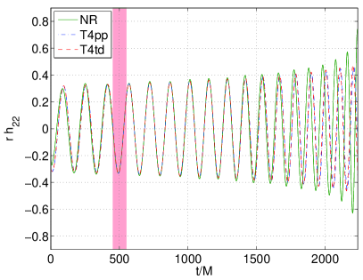
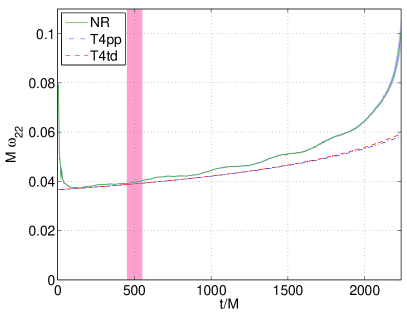
Figure 10: Comparison T4pp/T4td–NR, $r\,h_{22}$ (right) and $M\,\omega_{22}$ (left). The shaded red area at early time is the alignment region. A very thin shaded blue area (barely distinguishable on this scale) shows the uncertainty of NR data.

As a case study we focus on our best NR waveform extrapolated only in resolution, i.e. HH$\{23456\}$. Neglecting finite-extraction uncertainties does not particularly affect the conclusions, also because they decrease towards merger. As discussed extensively in Hannam et al. (2010b) the error estimates of Sec. IV based on the convergence analysis may not be the optimal ones to be used in PN comparison. If only a certain range of frequencies of the NR waveform is of interest, a phase error estimated on that range (i.e. by shifting in some way NR waves from different runs) may be less conservative and thus preferable for the specific application. However, such error estimates suffer of ambiguities related to the alignment procedure and we prefer not to pursue that method. For the purpose of this section is sufficient and justified to use the errors estimated in Sec. IV that can be, eventually, considered as an upper bound to the actual errors (see below).

Figure 10 shows the real part of the aligned waveforms (error bars are not shown there for clarity), and the GW frequencies with error bars. The alignment interval used for the analysis in the figure is $[t_{1},t_{2}]/M=[450,550]$, which minimizes the mismatch between the NR and T4td waveform as described above. Figure 11 shows the phase differences between the waveforms in time (left) and frequency (right) domain. The PN waveform maintains a good phasing for few GW cycles after the alignment region and up to $t/M\sim 1200$. At later times, phase differences with respect the PN evolution become positive and significant, the largest difference is the one with T4pp. At higher GW frequencies than $M\,\omega_{22}\sim 0.05$ the PN approximant significantly differ from NR waves, and the T4pp rapidly accumulates a phase difference of $\Delta\Phi_{22}\sim 2$ $rad$ at $M\,\omega_{22}\sim 0.07$ and of $\Delta\Phi_{22}\sim 4$ $rad$ at $M\,\omega_{22}\sim 0.1$. The T4td performs slightly better then T4pp at later times, but (not yet calculated) higher order tidal corrections are important . This is the central observation here: tidal interactions in the nonlinear regime dominate the dynamics and the GW emission at least during the last 5-6 orbits of the merger process. A similar conclusion can be drawn considering the waveform HH$\{2346\}$, but not for HH$\{236\}$. In the latter case the PN and NR signals are indistiguishable due to larger error bars.

As mentioned above, we did not perform a systematic study of different alignment procedures, but a certain dependence on the alignment interval was expected and observed. The phase differences given above are lower bounds, since they are determine by a minimization of the mismatch functional. In particular, dropping the step (iv) in the procedure outlined above and varying $t_{c}\in[0,900]\,M$, we estimated also an upper bound. The latter corresponds to an alignment interval centered at $t_{c}\sim 70\,M$ and the accumulated phase are $\Delta\Phi_{22}\sim 3$ $rad$ at $M\,\omega_{22}\sim 0.07$ and of $\Delta\Phi_{22}\sim 6$ $rad$ at $M\,\omega_{22}\sim 0.1$.

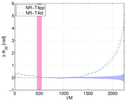
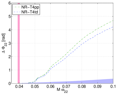
Figure 11: Phase differences T4pp/T4td-NR in time (left) and frequency domain (right). The shaded red area at early time is the alignment region. The shaded blue area is the uncertainty of NR data.

VI Conclusions

In this paper we have presented results about the accuracy of NR waveforms from BNS mergers and their comparison with PN methods. The simulations cover nine orbits of the late inspiral and the merger phase, they are the longest and most accurate BNS simulations to date, in terms of the resolution employed and the number of runs performed for a single initial configuration. The convergence of the waveforms and their uncertainties related to truncation errors and finite-radius extraction are discussed. For the first time in case of BNS merger waveforms, the accuracy standards for detection have been evaluated. The aim of the study is to assess the quality of NR waveforms in view of their future use to understand the physics of the merger and of tidal interactions or for data analysis purposes. As a first step in this direction, a comparison with the PN T4 waveforms has been presented.

NR waveforms are found to be convergent at second order rate during the inspiral and up to contact, i.e. until the last 1.5 orbits or, equivalently, for the GW frequencies $M\,\omega_{22}\lesssim 0.07$. Later an over-convergent behavior is observed, likely due to the numerical treatment of the matter and possibly also to the lowest resolution run employed in the self-convergence test. The uncertainties on the inspiral waves have been estimated by using Richardson extrapolation of different data sets and assuming the observed convergence rate where it is valid. finite-radius extraction affects were investigated by extrapolating the waves to null-infinity. Truncation errors increase towards the merger, when the amplitude of the GW become maximum. The maximum errors in phase and amplitude observed are reported in Tab. 2 for different extrapolations series. The errors related to finite-radius extraction decrease towards the merger and they are generically the smaller then truncation errors, but of the same order of magnitude of truncation errors in some relevant cases of waves extrapolated in resolution. Some of these results are compatible with the findings of Baiotti et al. (2011).

Accuracy standards have been evaluated using noise curves of ground-based detectors, and assuming minimal requirements. Results are reported in Tab. 3. Considering the most optimistic error-bars, extrapolated waveforms from five runs are effectual and faithful for detection with SNR $\varrho\lesssim 10$ for most of the configurations considered. Considering instead more conservative error-bars, or extrapolation in resolution with fewer runs, waveforms are neither effectual nor faithful for relevant SNRs.

These facts may affect some of the conclusions of previous works where errors of the NR waveforms were (not available and thus) neglected, but statements about the detectability of (small) effects (EoS, magnetic fields) were made. Our results should be taken into account and/or reproduced in future works employing NR waveforms for data analysis purposes or for comparison with analytic methods.

The NR data have been compared with the prediction of the PN T4 formula, both for point-particle (T4pp) and including all the analytically known tidal corrections (T4td). The comparison between the NR and the T4 waves has been carried out by aligning them in time and phase at low frequencies, and looking at the accumulated phase difference. The aligned T4pp waveform accumulates rapidly a significant dephasing of $\Delta\phi_{22}\sim 2$ at $M\,\omega_{22}\sim 0.07$, and $\Delta\phi_{22}\sim 4$ at $M\,\omega_{22}\sim 0.1$. These values can be considered lower bounds since in the comparison waves are aligned in such a way to minimize the mismatch and error-bars from the convergence test are employed. The inclusion of tidal corrections does not reduce the phase difference more than a fraction of a radiant. The results suggest that tidal interactions are very amplified in a strong field and nonlinear regime and play a significant role already during the last nine orbits. As already observed in Baiotti et al. (2011) the analytically known LO and NLO tidal terms in the T4 PN approximant are not sufficient to match the NR waveform.

In summary, our work indicates that NR waveforms from BNS are physically “reliable” because convergent and comparable with PN at sufficiently low frequencies. The measured uncertainties are such that the NR waveforms from BNS may not be sufficiently accurate for data analysis purposes, unless data extrapolated from several runs are employed. For data analysis applications, an error estimate based on relative as well as absolute comparisons (aligning/not-aligning the waveforms) will be relevant. A very careful evaluation of the waveform uncertainties is unavoidable for their use in quantitative studies.

Future work will be devoted to a more comprehensive comparison between the NR waves and analytic PN fitting models, either in the standard Taylor form or resummed one (EOB), to extend these results to different mass ratios and EoSs, and to the investigation of different grid setup and higher order methods for the treatment of the matter.

Appendix A Accuracy standards

In this appendix the accuracy standards used in this paper are discussed. We follow Cutler and Flanagan (1994); Miller (2005); Damour et al. (2011a); Lindblom et al. (2008); Lindblom (2009).

Given two real time series (waveforms), $h_{\rm x,m}(t)$, and their Fourier complex transform, $\tilde{h}_{\rm x,m}(f)$, the Wiener scalar product is defined as,

$$(h_{\rm x}|h_{\rm m})\equiv 4\Re\int_{0}^{\infty}df\frac{\tilde{h}_{\rm x}(f)\tilde{h}^{*}_{\rm m}(f)}{S_{\rm n}(f)}\ ,$$ (4)

where $S_{\rm n}(f)$ is the one-sided power spectral density of the detector noise. The (squared of the) norm associated to the Wiener product is $||h_{\rm x}||^{2}_{\rm w}\equiv(h_{\rm x}|h_{\rm x})$. The Wiener product is real and symmetric, the associated norm is positive definite. The Wiener product provides a measure in the waveform space Cutler and Flanagan (1994). The mismatch functional is defined as,

$$\mathcal{M}[h_{\rm m},h_{\rm x}]\equiv 1-\frac{(h_{\rm x}|h_{\rm m})}{||h_{\rm x}||_{\rm w}||h_{\rm m}||_{\rm w}},$$ (5)

and it is often employed to discuss accuracy standards for BBH NR waveforms, see e.g. Hannam et al. (2009); Reisswig et al. (2009a); Hannam et al. (2010a). In this work we will mainly focus on (the square of) the inaccuracy functional Damour et al. (2011a), defined as

$$\mathcal{I}^{2}[h_{\rm m},h_{\rm x}]=\frac{||h_{\rm m}-h_{\rm x}||_{\rm w}}{||h_{\rm x}||_{\rm w}}\ .$$ (6)

The inaccuracy functional has been considered for NR waveforms, for example, in MacDonald et al. (2011), and provides an equivalent measure to the mismatch functional.

Assuming an ideal detector (i.e. neglecting calibration errors), a waveform $h_{\rm m}$ (the “model”) is indistinguishable from the waveform $h_{\rm x}$ (the “exact”), if and only if their difference $\delta h=h_{\rm m}-h_{\rm x}$ satisfies,

$$||\delta h||_{\rm w}<1\ .$$ (7)

Eq. (7) represents an accuracy requirement for measurement purposes, and it determines the faithfulness of the model waveform. A less restrictive requirement can be given for detection purposes, and it is related to the effectualness of the model waveform. A sufficient condition is,

$$||\delta h||_{\rm w}<\sqrt{2\varepsilon_{\rm M}}\varrho\ ,$$ (8)

where $\varrho\equiv||h_{\rm x}||_{\rm w}$ is the optimal signal-to-noise ratio (SNR) and the constant $\varepsilon_{\rm M}$ set the accuracy level. We set in this work $\varepsilon_{\rm M}=0.005$ or $\varepsilon_{\rm M}=0.035$ as suggested in Lindblom et al. (2008) (see references therein).

Conditions (7) and (8) depend on the distance of the detector form the source. If they are written in term of the inaccuracy functional, the dependence on absolute scales can be moved to the right-hand-side and expressed only in term of the SNR. The accuracy requirements then read,

$$\mathcal{I}^{2}=\frac{||\delta h||_{\rm w}}{||h_{\rm x}||_{\rm w}}<\begin{cases}\varepsilon/\varrho&\text{faithful},\\ \sqrt{2\varepsilon_{\rm M}}&\text{effectual},\\ \end{cases}$$ (9)

where the functional dependence has been omitted for clarity. The level $\varepsilon<1$ is here set as $\varepsilon=0.5$. Equivalent conditions to Eq. (9) can be expressed in term of the L2 norm of the time domain signals Lindblom et al. (2008), however they are not considered here because they seem more restrictive than the frequency domain criteria.

In order to evaluate the accuracy of NR waveforms, one can consider $h_{\rm x}$ as the best waveform model (the extrapolated in resolution in our case), and construct $h_{\rm m}=h_{\rm x}+\delta h$ from the error estimates (the last resolution waveform in our case). The accuracy requirements in Eq. (9) then quantify the accuracy of the NR waveforms. In the analysis presented in the paper the integration interval $f\in[0,\infty]$ is approximated as $f\in[f_{0},f_{\rm max}]$, covering only the inspiral physical frequencies.

The Wiener product is computed by scaling the waveforms to physical units and to an effective distance, ${\rm D_{eff}}$, typically given in $100~{}Mpc$. From the code output $r\,h_{22}$, we: (i) recover $r\,h_{+}$ from the (2,2) multipole, using the expression for the spin weighted spherical harmonics, ${}^{-2}Y_{2\pm 2}(\theta,\phi)=\sqrt{5/(64\pi)}\exp(\pm i2\phi)(1\pm\cos\theta)^{2}$; and (ii) scale $r\,h_{+}$ to an effective distance. Assuming the radiation is emitted on the $z$ axis, perpendicularly to the orbital plane, one has,

$$rh_{+}(t) = r\ \Re\left({}^{-2}Y_{22}h_{22}+{}^{-2}Y_{2-2}h_{2-2}\right)$$

$$\simeq 0.6308\ r\ \Re\left(h_{22}\right)\ \ \ (\mbox{for}\ \theta=0\,,\ \phi=0)$$

$$h_{+}(t,D_{\rm eff}) = rh_{+}(t)\ {GM_{\odot}c^{-2}}\ \left(\frac{{\rm D_{eff}}}{Mpc}\right)^{-1}$$

$$\simeq rh_{+}(t)\ 4.7857\times 10^{-20}\ \left(\frac{{\rm D_{eff}}}{Mpc}\right)^{-1}\ .$$

Unit conversion: $1~{}Mpc\simeq 3.08568025\times 10^{24}$ $cm$, $GM_{\odot}c^{-2}\simeq 1.47670133\times 10^{5}$ $cm$.