Entropy-limited higher-order central scheme for neutron star merger simulations

Abstract

Numerical relativity simulations are the only way to calculate exact gravitational waveforms from binary neutron star mergers and to design templates for gravitational-wave astronomy. The accuracy of these numerical calculations is critical in quantifying tidal effects near merger that are currently one of the main sources of uncertainty in merger waveforms. In this work, we explore the use of an entropy-based flux-limiting scheme for high-order, convergent simulations of neutron star spacetimes. The scheme effectively tracks the stellar surface and physical shocks using the residual of the entropy equation thus allowing the use of unlimited central flux schemes in regions of smooth flow. We perform the first neutron star merger simulations with such a method and demonstrate up to fourth-order convergence in the gravitational waveform phase. The scheme reduces the phase error up to a factor five when compared to state-of-the-art high-order characteristic schemes and can be employed for producing faithful tidal waveforms for gravitational-wave modelling.

I Introduction

The detection of gravitational waves (GWs) from binary neutron star (BNS) merger events by the LIGO-Virgo collaboration opened the way to observationally probe NS matter with GW signals Abbott et al. (2017, 2018, 2019, 2020). Key to this endeavour is the availability of merger waveforms from numerical relativity (NR) simulations that accurately resolve tidal effects and allows the design of sophisticated waveform templates Damour et al. (2012); Baiotti et al. (2010); Bernuzzi et al. (2012a); Read et al. (2013); Bernuzzi et al. (2015); Hinderer et al. (2016); Dietrich et al. (2017a). Current tidal waveform templates have been shown to be inaccurate (unfaithful) for the inference of tidal parameters at the signal-to-noise ratios that would otherwise allow a precision measurement Gamba et al. (2021). The main source of inaccuracy is the modelling of tidal interactions toward merger and it is related to the lack of sufficiently accurate NR simulations. This is a critical open issue for science with advanced detectors and an urgent problem to solve in view of third-generation Kalogera et al. (2021).

Current state-of-the-art NR waveforms for modeling tidal interactions span about ten orbits to merger and have typical accumulated phase errors below one radiant e.g. Bernuzzi et al. (2012a); Radice et al. (2014a); Hotokezaka et al. (2015); Bernuzzi and Dietrich (2016); Dietrich et al. (2018b). Early studies pointed to numerical dissipation in relativistic hydrodynamics (GRHD), to the numerical handling of the stellar surfaces and to the slow convergence of high-resolution shock-capturing (HRSC) as the main difficulties towards the computation of precise waveforms Baiotti et al. (2009); Thierfelder et al. (2011); Bernuzzi et al. (2012b, a); Hotokezaka et al. (2013). The primary goal is to assess waveforms’ error budget based on convergent data and rigorous self-convergence tests, that has been presented by few groups Thierfelder et al. (2011); Bernuzzi et al. (2012b); Radice et al. (2014a). Traditional finite volume methods for GRHD using linear reconstructions, the piece-wise parabolic method Colella and Woodward (1984); Martí and Müller (1996) or even third-order convex-essentially-non-oscillatory (CENO3) algorithm Liu and Osher (1998); Del Zanna, L. and Bucciantini, N. (2002) allows robust and successful simulations but do not produce convergent waveforms at affordable resolutions Giacomazzo et al. (2009); Thierfelder et al. (2011); Bernuzzi et al. (2012a); Radice et al. (2014b). Consequently, high-order (HO) numerical schemes based on fifth-order characteristic reconstructions of the GRHD fields Shu and Osher (1989) have been explored and represent the best methods available to date Radice et al. (2014a); Bernuzzi and Dietrich (2016). HO schemes allow the computation of convergent waveforms but none of the schemes tested so far achieves the formal high-order accuracy expected for smooth flow. Nonetheless, the direct data comparison between two independent codes indicate good agreement within the estimated errorbars Nagar et al. (2018) (see Appendix D). While convergent waveform can be obtained, the computational cost of producing GW with sub-radiant accuracy over multiple orbits and to merger remains rather high Radice et al. (2015); Dietrich et al. (2018b).

In the present work we explore further the potential of a method that started as an artificial viscosity method Guermond and Pasquetti (2008) and developed through the years to a flux-limiting method Guercilena et al. (2017). The central idea of this method is to use a physical quantity as an indicator of the location of abnormal non-smooth regions like shocks, rarefactions etc. Entropy is an ideal candidate for this role as shocks are irreversible processes and thus increase the overall entropy of the system. Therefore, entropy can be used to flag the presence of non-smooth features in the solution space. The idea of using the entropy to design numerical methods for non-linear conservation laws is not new though. For example it is shown in Andrews and Morton (1998); Puppo (2004) that the entropy production can be used as a posteriori shock indicator and therefore it is extremely useful in the shock tracking. The authors in Guermond and Pasquetti (2008); Guermond et al. (2011) used the aforementioned idea to design a novel class of high-order numerical approximations to non-linear conservation laws by adding a degenerate non-linear dissipation to the numerically discretized system. The additional non-linear viscosity term is based on the local size of the entropy production. By making the numerical diffusion proportional to the entropy production in strong shocks, large numerical dissipation is added in the shock regions and almost no dissipation in the regions where the solution is smooth. This close interplay between the notions of entropy and viscosity gave the name entropy-viscosity (EV) to this method.

In Guercilena et al. (2017) the EV method was incorporated in a HRSC method and extended to special and general relativistic hydrodynamics. Accordingly, the definitions of the entropy and viscosity were generalised and the viscosity was employed to drive a flux-limiting scheme rather than generating additional viscous terms in the hydrodynamical equations. The equations of GRHD are not modified anymore by the inclusion of additional viscosity related terms. Instead, a flux-limiting strategy is employed, i.e. the numerical fluxes are computed using an unlimited high-order stencil complemented by a first-order, non-oscillatory local Lax-Friedrichs (LLF) flux in regions of non-smooth flow. The high-order and low-order fluxes are linearly combined using local weights that are determined by i) an entropy-based shock detector criterion (based on the residual of the entropy equation) and ii) a positivity preserving limiter Hu et al. (2013). This hybrid scheme was named entropy-limited hydrodynamics (ELH). It has been shown effective in capturing shocks and discontinuities in special relativistic shock tubes as well as in producing stable evolutions of single neutron star by properly handling stellar surface effects. Guercilena et al. (2017) also points out shortcomings of the method: small spurious oscillations are observed in the blast wave 2 test, while neutron star evolutions show a spurious direction-dependent feature that breaks spherical symmetry.

In the present work, we build upon the existing machinery of the ELH method. While keeping loyal to the basic features of the method, we extend and generalise some of its aspects and modify or even drop some others. Most noticeably we drop the use of the positivity preserving limiter Hu et al. (2013) and define the weights of the fluxes directly from the entropy produced by the system under investigation. Another notable amendment is that we allow the unfiltered high-order flux to be supplemented by general stable low- or high-order fluxes. In addition, the ELH is simplified by completely defining the free parameters inherent in the method. In light of the above quantitative differences with the ELH method we name the scheme developed in the present work entropy based flux-limiter (EFL) method as it describes exactly what we have developed: a genuine entropy based flux-limiter. The new, EFL scheme remains robust in handling the special relativistic and the single neutron star tests, notably improving the shortcoming of the previous implementation. Moreover, we successfully apply for the first time the scheme to BNS simulations.We discuss high-order convergence in the inspiral-merger GWs and future prospect for producing faithful waveforms for GW modeling.

The article is structured as follows. In Sec. II, after briefly summarising the equation of GRHD, we discuss theoretical and numerical aspects of our method. Sec. III includes our results for the standard benchmark tests of special relativity, and in Sec. IV the performance of our method is tested against three-dimensional general relativistic single NS configurations. Our main results are presented in Sec. V, where the first BNS evolutions with a method based on the entropy production can be found. Finally, we conclude in Sec. VII.

Throughout this work we use geometric units. We set $c=G=1$ and the masses are expressed in terms of solar masses $M_{\odot}$.

II Method

II.1 General relativistic hydrodynamics

The evolution of a relativistic fluid in the presence of a non-trivial gravitational field $g_{\mu\nu}$ is described by the local conservation laws of the energy-momentum tensor $T_{\mu\nu}$ and of the rest-mass current $J^{\mu}=\rho\,u^{\mu}$,

$$\nabla_{\mu}T^{\mu\nu}=0\quad\mathrm{and}\quad\nabla_{\mu}J^{\mu}=0,$$ (1)

respectively. Above $\nabla$ denotes the covariant derivative compatible with $g_{\mu\nu}$, $\rho$ is the rest-mass density and $u^{\mu}$ is the 4-velocity of the fluid. The evolution equations (1) in the 3+1 formalism Alcubierre (2008) can be written as a system of PDEs in conservation form Banyuls et al. (1997)

$$\partial_{t}\textbf{Q}+\partial_{i}\textbf{F}^{i}=\textbf{S},$$ (2)

where the summation is performed over the spatial dimensions $i=\{x,y,z\}$ and the vector Q of the conserved variables reads

$$\textbf{Q}=\sqrt{\gamma}\begin{bmatrix}D\\ S_{j}\\ \tau\end{bmatrix}:=\sqrt{\gamma}\begin{bmatrix}\rho\,W\\ \rho\,h\,W^{2}\,u_{j}\\ \rho\,h\,W^{2}-p-\rho\,W\end{bmatrix}$$ (3)

where $S_{j}=\{S_{x},S_{y},S_{z}\}$, $p$ is the pressure, $h$ is the specific enthalpy $h=1+\epsilon+p/\rho$ with $\epsilon$ the specific internal energy, $W=(1-u_{i}\,u^{i})^{1/2}$ is the Lorentz factor and $\gamma$ is the determinant of the 3-metric $\gamma_{ij}$ resulting from the 3+1 decomposition of ($\mathcal{M},g_{\mu\nu}$). The vector $\textbf{F}^{i}$ of the physical fluxes is

$$\textbf{F}^{i}=\sqrt{\gamma}\begin{bmatrix}(\alpha\,u^{i}-\beta^{i})\,D\\ (\alpha\,u^{i}-\beta^{i})\,S_{j}+\alpha\,p\,\delta^{i}_{j}\\ (\alpha\,u^{i}-\beta^{i})\,\tau+\alpha\,p\,u^{i}\end{bmatrix},$$ (4)

where $\alpha$ is the lapse function, $\beta^{i}$ the shift vector and $\delta^{i}_{j}$ the Kronecker delta. Finally, the vector S of the sources has the form

$$\textbf{S}=\alpha\,\sqrt{\gamma}\begin{bmatrix}0\\ \Gamma^{\mu}_{\nu j}T^{\nu}_{\mu}\\ \alpha\left(T^{0\mu}\partial_{\mu}\ln\alpha-\Gamma^{0}_{\mu\nu}T^{\mu\nu}\right)\end{bmatrix},$$ (5)

where $\Gamma^{\rho}_{\mu\nu}$ are the Christoffel symbols associated with the metric $g_{\mu\nu}$. Notice that the system (2) reduces to its special relativistic counterpart in the limit $(\alpha,\beta^{i},\gamma_{ij})\rightarrow(1,0,\delta_{ij})$, i.e. when $\textbf{S}\rightarrow 0$.

In order to close the underdetermined system (2) one needs an equation of state (EoS) that specifies the pressure in terms of the density and the internal energy, i.e $p=p(\rho,\epsilon)$. Specifically, for the special relativistic tests of Sec. III we use a $\Gamma$-law EoS,

$$p=(\Gamma-1)\rho\,\epsilon,$$ (6)

with $\Gamma$ the adiabatic index. The neutron star matter of the single neutron star evolutions of Sec. IV is also modelled by a $\Gamma$-law EoS (6). Finally, the matter of the neutron stars comprising the binaries of Sec. V is described by either a $\Gamma$-law EoS (6) or by a more realistic SLy EoS Douchin and Haensel (2001). The latter is implemented by a piecewise polytrope fit Read et al. (2009), and thermal effects are modeled by an additive pressure contribution given by the $\Gamma$-law EoS with $\Gamma=1.75$ Shibata et al. (2005); Bauswein et al. (2010); Thierfelder et al. (2011).

II.2 EFL method

In the present work the entropy-viscosity (EV) method Guermond and Pasquetti (2008); Guermond et al. (2011) is used as a flux limiting scheme in the spirit of Guercilena et al. (2017). In Guercilena et al. (2017) the original EV method was reformulated as an entropy based flux-limiter and extended to special and general relativistic hydrodynamics. The basic idea of the ELH method consists of expressing the numerical fluxes resulting from the spatial discretisation of (2) as a superposition of an (unstable) high- and a (stable) low-order flux, where the weight dictating the transition between the two fluxes is computed based on the entropy produced in the system under investigation. The entropy of the system is used as a “shock detector” that indicates when to switch from the high-order scheme to the low-order one.

The EFL method follows in broad lines the exposition in Guercilena et al. (2017), but adds some novelties to the already existing scheme. One of the main differences is that we do not use the positivity-preserving limiter Radice et al. (2014b) in the definition of the transition weight $\theta$. Another key development is that the LO flux here is composed of a non-oscillatory high-order scheme, namely a finite volume method with high-order reconstruction (CENO3, WENO, etc.). In this way the chances that the resulting hybrid flux can achieve high-order convergence rates are maximised. Finally, the handling of the tunable constants is extremely simplified, see last paragraph of the current section for further details.

We start by approximating the spatial derivative of the $x$ component, $\textbf{F}^{x}$, of the physical flux (4) appearing in (2) with the conservative finite-difference formula

$$\partial_{x}F^{x}_{i}=\frac{\hat{f}_{i+1/2}-\hat{f}_{i-1/2}}{h},$$ (7)

where $F^{x}$ is any one of the components of $\textbf{F}^{x}$ with $F^{x}_{i}=F^{x}(x_{i})$, $\hat{f}_{i\pm 1/2}$ are the numerical fluxes at the cell interfaces and $h$ is the spatial grid spacing.

Next, we split the numerical fluxes on the r.h.s. of (7) into two contributions, see also Guercilena et al. (2017): one from a HO scheme and one from a low-order (LO) stable scheme, i.e.

$$\hat{f}_{i\pm 1/2}=\theta_{i\pm 1/2}\hat{f}^{\,\mathrm{HO}}_{i\pm 1/2}+(1-\theta_{i\pm 1/2})\hat{f}^{\,\mathrm{LO}}_{i\pm 1/2},$$ (8)

where the continuous parameter $\theta\in[0,1]$ plays the role of a weight that indicates how much from each scheme to use at every instance. The HO flux $\hat{f}^{\,\mathrm{HO}}$ is built using the Rusanov Lax-Friedrichs flux-splitting technique and performing the reconstruction on the characteristic fields Mignone et al. (2010); Bernuzzi and Dietrich (2016). A fifth-order central unfiltered stencil (CS5) is always used for reconstruction. The LO flux $\hat{f}^{\,\mathrm{LO}}$ is approximated by the LLF central scheme with reconstruction performed on the primitive variables Thierfelder et al. (2011). Primitive reconstruction is performed with a variety of low- and high-order reconstruction schemes. (Notice that we generalise the traditional notion of a flux-limited scheme where $\hat{f}^{\,\mathrm{LO}}$ is always a LO monotone flux Toro (1999); Hesthaven (2018).) A list of the ones used in the present work follows. Godunov’s piecewise constant reconstruction scheme (GODUNOV) Godunov (1959); the second-order linear total variation diminishing (LINTVD) interpolation based on “minmod” and “monotonized centered” slope limiters Harten (1983); Toro (1999); the third-order convex-essentially-non-oscillatory (CENO3) algorithm Liu and Osher (1998); Del Zanna, L. and Bucciantini, N. (2002); and the fifth-order weighted-essentially-non-oscillatory finite difference schemes WENO5 Jiang (1996) and WENOZ Borges et al. (2008). As it was mentioned above, this is a basic difference of the EFL method with the one proposed in Guercilena et al. (2017); therein a first-order Lax-Friedrichs flux was used exclusively as the LO flux.

The computation of $\theta$ is based on the so-called entropy production function $\nu$: a quantity that depends on the amount of entropy produced in the system. Explicitly, the relation between $\theta$ and $\nu$ is

$$\theta_{i\pm 1/2}=1-\frac{1}{2}(\nu_{i}+\nu_{i\pm 1}).$$ (9)

Below, we summarise how to compute $\nu$.

In order to quantify the relation between $\nu$ and the entropy produced by the system under investigation, we define the specific entropy (entropy per unit mass) of any piecewise polytropic EoS as

$$s=\ln\left(\frac{p}{\rho^{\Gamma}}\right),$$ (10)

where the pressure is computed in accordance with the EoS in use.

Following Guercilena et al. (2017), we employ the second law of thermodynamics to define the entropy residual:

$$\mathcal{R}=\nabla_{\mu}(s\,\rho\,u^{\mu})\geq 0,$$ (11)

which provides a quantitative estimation of the rate of the entropy produced by the system under study. Using the continuity equation and writing the 4-velocity $u^{\mu}$ in terms of the fluid 3-velocity $\upsilon^{i}$, the above expression can be written Guercilena et al. (2017) in terms of the time and spatial derivatives of the specific entropy as

$$\mathcal{R}=\frac{\rho W}{\alpha}\left(\partial_{t}s+(\alpha\,\upsilon^{i}-\beta^{i})\partial_{i}s\right).$$ (12)

In order to simplify the definition of the constant $c_{E}$, see discussion below, we suppress the multiplication factor $\frac{\rho W}{\alpha}$ and replace $\mathcal{R}$ by

$$R=\partial_{t}s+(\alpha\,\upsilon^{i}-\beta^{i})\partial_{i}s,$$ (13)

which amounts to a rescaling of $\mathcal{R}$ so that the coefficient of $\partial_{t}s$ is equal to one.

Finally, we define the entropy production function in terms of the rescaled entropy residual $R$,

$$\nu_{E}=c_{E}|R|,$$ (14)

where $c_{E}$ is a tunable constant used to scale the absolute value of $R$. In all our simulations we did not have to tune $c_{E}$, its value was set to unity, i.e. $c_{E}=1$. Keeping in mind that the parameter $\theta$ cannot exceed unity, we have to impose a maximum value of $\nu_{\rm max}=1$ for the entropy production function in order to ensure that the rhs of (9) does not exceed the range $[0,1]$. Accordingly, the entropy production function entering (9) is given by

$$\nu=\min\left[\nu_{E},1\right].$$ (15)

Comparing directly with Guercilena et al. (2017), note the following differences. In the present work, we use (9) directly for the definition of $\theta$, while Guercilena et al. (2017) adds a condition for positivity preservation. We define $R$ as in (13), while Guercilena et al. (2017) considers $\mathcal{R}=\frac{\rho W}{\alpha}R$. Finally, we define the entropy production function as $\nu_{E}=c_{E}|R|$, while in Guercilena et al. (2017) $\nu_{E}$ is multiplied with $\Delta_{m}$, where $\Delta_{m}$ is the mesh spacing.

In other words, based on various numerical experiments we found it advantageous to remove the factor $\frac{\rho\,W\Delta_{m}}{\alpha}$ from the definition of the entropy production function $\nu_{E}$ compared to ELH. We study results for $c_{E}=1$ in detail, while $c_{E}=\frac{\rho\,W\Delta_{m}}{\alpha}$ is considered in Guercilena et al. (2017). In the EFL method proposed here, there is no direct resolution dependence, and the entropy production has been normalized to the scale of $\partial_{t}s$.

II.3 Numerical implementation

The finite differencing code BAM Brügmann et al. (2008); Thierfelder et al. (2011); Dietrich et al. (2015b); Bernuzzi and Dietrich (2016) is used to solve numerically the system of equations discussed in subsection II.1 coupled to the metric equations for General Relativity. The EFL method presented in subsection II.2 has been implemented into BAM and is part of its infrastructure. BAM uses the method-of-lines with Runge-Kutta (RK) time integration and finite differences for the approximation of spatial derivatives. The value of the Courant-Friedrich-Lewy (CFL) condition is set to 0.25 for all runs.

The numerical domain contains a mesh made of a hierarchy of cell-centered nested Cartesian boxes and consists of $L$ refinement levels $l=0,\dots,L-1$ ordered with increasing resolution. Each refinement level is made out of one or more equally spaced Cartesian grids with grid spacing $h_{l}$. There are $n$ points per direction on each grid plus a certain number of buffer points on each side. (For simplicity, we always quote grid sizes without buffer points.) The resolution between two consecutive levels is doubled such that the grid spacing at level $l$ is $h_{l}=h_{0}/2^{l}$, where $h_{0}$ is the grid spacing of the coarsest level. The inner levels move in accordance with the moving boxes technique, while the outer levels remain fixed. The number of points in one direction of a moving level can be set to a different value than the number of points of a fixed level. The coordinate extent of a grid at level $l$ entirely contains grids at any level greater than $l$. The moving refinement levels always stay within the coarsest level. For the time evolution of the grid the Berger-Oliger algorithm is employed enforcing mass conservation across refinement boundaries Dietrich et al. (2015b); Berger and Oliger (1984). Restriction and prolongation is performed for the matter fields with a fourth-order WENO scheme and for the metric fields with a sixth-order Lagrangian scheme. Interpolation in Berger-Oliger time stepping is performed at second-order.

For the numerical implementation of the EFL method the BAM routines computing the numerical fluxes had to be modified in order to accommodate the hybrid flux (8). In order to compute the entropy production (13) we have to approximate the time and spatial derivatives of the specific entropy. We use finite differences to do so. Specifically, the spatial derivatives are approximated, as in Guercilena et al. (2017), with a standard centered finite-difference stencil of order $p+1$ or higher, where $p$ is the order of the stencil used to approximate the physical fluxes. (In the present work we use $p=5$.) With this restriction it is ensured that the entropy production function $\nu$ converges to zero faster than the overall convergence of the scheme. The time derivative is also approximated with finite differences. We employ a third-order one-sided stencil by using, at every Runge-Kutta iteration, the current value of the specific entropy and the values at the three previous timesteps. The fact that we manage to achieve higher than third-order convergence in the majority of our simulations can be possibly attributed to the dominance of the spatial error over the time discretization error.

The derivatives of the metric components are approximated by fourth-order accurate finite-differencing stencils. In addition, sixth-order artificial dissipation operators are employed to stabilize noise from mesh refinement boundaries. The general relativistic hydrodynamic equations (2) are solved by means of a high-resolution-shock-capturing method Thierfelder et al. (2011) based on primitive reconstruction and the aforedescribed high-order entropy limited scheme for the numerical fluxes. In the present work spacetime is dynamically evolved using either the BSSNOK Nakamura et al. (1987); Shibata and Nakamura (1995); Baumgarte and Shapiro (1999) or the Z4c Bernuzzi and Hilditch (2010); Hilditch et al. (2013) evolution scheme.

Vacuum regions are simulated with the introduction of a static, low-density, cold atmosphere in the vacuum region surrounding the star Thierfelder et al. (2011). The atmosphere density is defined as

$$\rho_{\rm atm}=f_{\rm atm}\,\mathrm{max}\,\rho(t=0).$$ (16)

All grid points with rest-mass density below a threshold value $\rho_{\rm thr}=f_{\rm thr}\rho_{\rm atm}$ are set automatically to $\rho_{\rm atm}$. Transition to low-density regions is one of the main sources of error in NS simulations. This is a common feature in all current numerical relativity implementations of NS dynamics. To deal with this challenging feature they also make use of similar assumptions and algorithms at low densities as those employed here. We leave it to future work to investigate whether the advantages of the atmosphere and vacuum treatment of Poudel et al. (2020), which improved mass conservation and accuracy of ejecta in that case study, can be combined with the new flux-limiting scheme. In the present work, we use the standard atmosphere treatment implemented in BAM Thierfelder et al. (2011), as our aim is to compare the performance of the newly developed entropy based flux-limiting scheme with our current best high-order flux scheme Bernuzzi and Dietrich (2016).

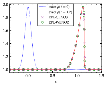
Figure 1: Simple wave. Numerical solution of the rest-mass density with $n=800$ grid-points and CFL factor 0.125 for the reconstruction schemes CENO3 (using purple $\times$) and WENOZ (using green $\circ$). The initial profile and the exact solution are also included using dashed blue and solid red lines, respectively.

III Special relativistic 1D tests

In this section a number of special relativistic one-dimensional tests are performed.

III.1 Simple wave

Table 1: Convergence results for the 1D simple wave test at $t=0.6$. $L_{1}$ and $L_{2}$ are normalised norms and the convergence rate is calculated as the $\log_{2}$ of the ratio of two successive normalised norms.

Scheme	n	$L_{1}$	Conv.	$L_{2}$	Conv.
EFL-WENO5	200	5.8e-04	–	1.9e-04	–
	400	2.6e-05	4.47	7.6e-06	4.66
	800	1.2e-06	4.41	2.6e-07	4.87
	1600	6.4e-08	4.26	6.9e-09	5.22
	3200	7.7e-09	3.05	3.6e-10	4.28
EFL-WENOZ	200	5.5e-04	–	1.8e-04	–
	400	2.6e-05	4.42	7.5e-06	4.57
	800	1.2e-06	4.39	2.6e-07	4.87
	1600	6.4e-08	4.26	6.9e-09	5.22
	3200	7.7e-09	3.05	3.6e-10	4.28
EFL-CENO3	200	6.9e-04	–	2.3e-04	–
	400	3.1e-05	4.50	8.5e-06	4.79
	800	1.5e-06	4.37	2.6e-07	5.01
	1600	9.1e-08	4.01	7.7e-09	5.09
	3200	1.1e-08	3.10	4.8e-10	4.01
EFL-LINTVD	200	1.0e-03	–	3.6e-04	–
	400	3.4e-05	4.88	1.0e-05	5.14
	800	1.4e-06	4.57	2.9e-07	5.14
	1600	1.0e-07	3.79	1.0e-08	4.84
	3200	1.3e-08	3.00	7.6e-10	3.76
HO-WENOZ	200	4.4e-04	–	1.3e-04	–
	400	2.8e-05	3.98	7.2e-06	4.16
	800	1.2e-06	4.53	2.6e-07	4.81
	1600	4.5e-08	4.73	6.5e-09	5.30
	3200	5.7e-09	2.98	2.8e-10	4.57

The relativistic simple wave is used as a first check of the accuracy and of the convergence properties of the EFL method. Although, simple waves start off from smooth initial data, their non-linear nature leads to the development of shocks at some point during their evolution. These tests have been discussed in Liang (1977); Anile (1990). Here, we use the simple wave described in Bernuzzi and Dietrich (2016), therein the initial velocity profile is of the form

$$\upsilon=a\,\Theta(|x|-X)\sin^{6}\left(\frac{\pi}{2}\left(\frac{x}{X}-1\right)\right),$$ (17)

where $\Theta(x)$ is the Heaviside function, $a=0.5$ and $X=0.3$. During the evolution the smooth initial profiles of all primitive variables become steeper and steeper and at around $t\simeq 0.63$ they form a shock. We use exactly the same numerical set-up with Bernuzzi and Dietrich (2016), i.e. our one-dimensional computational domain spans the interval $x\in[-1.5,1.5]$, RK4 is used as time-integrator and a CFL factor of 0.125 has been chosen. Fig. 1 depicts the simple wave at $t=1.2$ for a resolution of 800 grid-points ($h=0.00375$) for a high-order WENOZ and a lower-order CENO3 reconstruction scheme. (The behaviour of the other two reconstruction schemes used in this work is identical to the one depicted by Fig. 1.) By inspection, all schemes reproduce the correct physics. Tab. 1 contains the results of the convergence analysis of the EFL schemes of Fig. 1 at $t=0.6$ (just before the shock forms). As a reference the HO-WENOZ scheme developed in Bernuzzi and Dietrich (2016) is also included in Tab. 1—this is the high-order scheme that we use to approximate the HO flux $\hat{f}^{\,\mathrm{HO}}$ in (8), but with WENOZ (instead of CS5) for the reconstruction of the characteristic variables. All schemes converge to the exact solution with the expected convergence rate.

III.2 Sod shock-tube

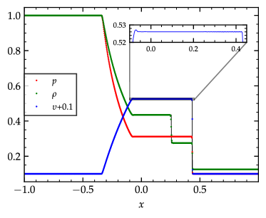
Figure 2: Profiles of the rest-mass density (green •), velocity (blue •) and pressure (red •) for the special-relativistic Sod test at $t=0.6$. Top: WENO5 reconstruction. Bottom: GODUNOV reconstruction. The solution is computed on a grid of 1600 points with resolution $\Delta x=1.25\times 10^{-3}$. Solid black lines are the exact solutions.

We move on now to the standard Riemann problems used as benchmarks in special relativistic hydrodynamics. Our first test is the relativistic version of Sod’s shock-tube problem Sod (1978). Assuming a simple ideal fluid EoS of the form (6) with adiabatic index $\Gamma=1.4$, the discontinuous initial data for the pressure $p$, the rest-mass density $\rho$, the velocity $\upsilon$, and the specific energy $\epsilon$ read

$$(p_{L},\rho_{L},\upsilon_{L},\epsilon_{L}) =(1,1,0,2.5),$$ (18)

$$(p_{R},\rho_{R},\upsilon_{R},\epsilon_{R}) =(0.1,0.125,0,2).$$

During the evolution the initial discontinuity at $x=0$ splits into a shock wave followed by a contact discontinuity, both travelling to the right, and a rarefaction wave travelling to the left.

Fig. 2 depicts our results at time $t=0.6$ for the best behaving high-order WENO5 and low-order GODUNOV reconstruction schemes at resolution $\Delta x=1.25\times 10^{-3}$. It is evident from Fig. 2 that the high-order scheme reproduces all the features of the Sod shock-tube quite accurately. A closer examination of the plots reveals the existence of small wiggles on the horizontal parts between the tail of the rarefaction and the shock; see, on the top panel of Fig. 2, the inset zoomed-in view of the horizontal portion of the velocity profile in question. The maximum amplitude of these wiggles is of the order of $\sim 10^{-3}$. The use of the low-order scheme prevents the appearance of these small wiggles but smears out considerably the profiles of the primitive variables, especially around the contact discontinuity. However, whichever scheme is used (low- or high-order) the oscillations at the discontinuities observed in Guercilena et al. (2017) are not present here.

III.3 Blast waves

III.3.1 Blast wave 1

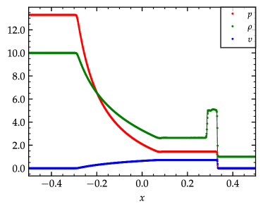
Figure 3: Profiles of the rest-mass density (green •), velocity (blue •) and pressure (red •) for the special-relativistic blast wave 1 test Marti and Müller (1999) at $t=0.4$. Top: WENO5 reconstruction. Bottom: GODUNOV reconstruction. The solution is computed on a grid of 800 points with resolution $\Delta x=1.25\times 10^{-3}$. Solid black lines are the exact solutions.

We continue now with more challenging shock-tube tests. We start with the relativistic blast wave 1 test described in Marti and Müller (1999). For an ideal EoS (6) with adiabatic index $\Gamma=5/3$ the initial values of the primitive variables read

$$(p_{L},\rho_{L},\upsilon_{L},\epsilon_{L}) =(13.33,10,0,1.995),$$ (19)

$$(p_{R},\rho_{R},\upsilon_{R},\epsilon_{R}) =(0,1,0,0).$$

The above data is evolved with the RK3 time integrator and a CFL factor 0.25 on a numerical grid that spans the domain $[-0.5,0.5]$ along the x-axis. The numerical domain is covered with 800 grid-points (resolution $1.25\times 10^{-3}$). The numerical solutions at $t=0.4$ are depicted in Fig. 3. The best performing high- and low-order schemes for the present shock-tube test are the WENO5 and GODUNOV reconstruction schemes, respectively. Both capture on a quite satisfactory level the main features of the exact solutions.

III.3.2 Blast wave 2

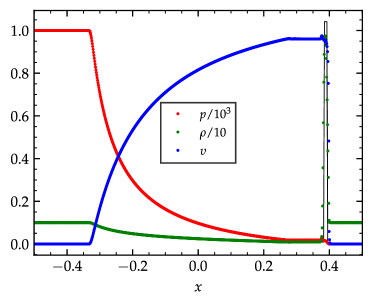
Figure 4: Profiles of the rest-mass density (green •), velocity (blue •) and pressure (red •) for the special-relativistic blast wave 2 test Marti and Müller (1999) at $t=0.4$. Top: WENO5 reconstruction. Bottom: GODUNOV reconstruction. The solution is computed on a grid of 800 points with resolution $\Delta x=1.25\times 10^{-3}$. Solid black lines are the exact solutions.

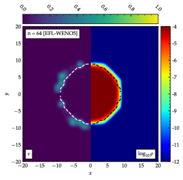
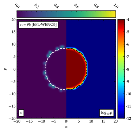
Figure 5: Two-dimensional profiles of the rest-mass density $\rho$ (right half of the plots) and entropy production function $\nu$ (left half of the plots) for a static TOV star in a dynamical spacetime with $\Gamma$-law EoS at $t=1000$. Top (left to right): CENO3, WENO5 and WENOZ reconstruction schemes with $n=128$. Bottom (left to right): The WENO5 scheme with increasing resolution of 64, 96 and 128 grid points, respectively. The other two schemes show similar behaviour. Dashed lines denote the surface of the NS at $t=0$.

Our final shock-tube test is the blast wave 2 test Marti and Müller (1999), where the discontinuity in the initial data of the pressure and the specific energy is of the order of $10^{5}$. The initial values of the primitive variables in this rather extreme scenario are the following

$$(p_{L},\rho_{L},\upsilon_{L},\epsilon_{L}) =(1000,1,0,1500),$$ (20)

$$(p_{R},\rho_{R},\upsilon_{R},\epsilon_{R}) =(0.01,1,0,0.015).$$

We assume again an ideal EoS (6) with adiabatic index $\Gamma=5/3$. The numerical solutions resulting from the evolution of (20) are computed on the domain $[-0.5,0.5]$ (resolution $1.25\times 10^{-3}$) with the RK3 integrator and a CFL factor of 0.25. The numerical solutions at $t=0.4$ are presented in Fig. 4. Therein the best behaving high- and low-order reconstruction schemes are presented and compared to the exact solution. Notice the small wiggle appearing on the profiles of the velocity and pressure close to the shock. It is definitely not an oscillation but some kind of by-product of the EFL method as its location coincides with a peak of the entropy production function $\nu$. Apart from this feature the EFL simulations reproduce to a fairly satisfactory degree all the features of the exact solutions.

IV Single star evolutions

Next, in order to test the performance of the EFL method in a three-dimensional general relativistic setting, we study the evolution of single NS spacetimes. These are very challenging tests as the stationarity of the stars favours the accumulation and growth of errors, especially around the location of the surface where the gradient of the hydrodynamical variables experience an abrupt change. Unavoidably, the overall accuracy of the simulations is affected. At the same time, these tests provide us with the exact solution that allows us to study the convergence properties of the numerical solutions in detail. We compare the performance of the EFL method with different reconstruction schemes. Finally, our results are compared with those of Guercilena et al. (2017); Bernuzzi and Dietrich (2016). For comparison we use the results obtain with i) a second-order scheme (LLF-WENOZ) that uses the LLF scheme for the fluxes and WENOZ for primitive reconstruction Thierfelder et al. (2011) and ii) a “hybrid” algorithm (HO-LLF-WENOZ) that employs the high-order HO-WENOZ scheme above a certain density threshold $\rho_{\mathrm{hyb}}$ and switches to the standard second-order LLF-WENOZ method below $\rho_{\mathrm{hyb}}$ Bernuzzi and Dietrich (2016).

Table 2: Grid configurations of single star simulations. Columns (left to right): name of simulation, $L$: number of fixed refinement levels, $n$: number of points per direction, $h_{L-1}$: resolution per direction in the finest level $l=L-1$, $h_{0}$: resolution per direction in the coarsest level $l=0$.

Name	$L$	$n$	$h_{L-1}$	$h_{0}$
TOV	3	64	0.281	1.125
	3	96	0.188	0.750
	3	128	0.141	0.563
RNS	3	64	0.422	1.688
	3	96	0.281	1.125
	3	128	0.211	0.845

In the following, we evolve stable rotating or non-rotating neutron stars Oppenheimer and Volkoff (1939) in a dynamically evolved spacetime. The NS matter is here described by a $\Gamma$-law EoS with $\Gamma=2$. The grid is composed of three fixed refinement levels. Simulations are performed at resolutions $n=(64,96,128)$ points leading to a grid spacing $h$ that depends on the specific setting of the NS under investigation. For each NS configuration the resolution is explicitly given in Tab. 2. It is ensured that the NS is entirely covered by the finest box at any given resolution. Radiative (absorbing) boundary conditions are used for all single star simulations.

IV.1 TOV star

Tolmann-Oppenheimer-Volkoff (TOV) initial data are constructed using a $\Gamma=2$ polytrope model with gravitational mass $M=1.4$, baryonic mass $M_{b}=1.506$ and central rest-mass density $\rho_{c}=1.28\times 10^{-3}$. The spacetime is dynamically evolved and the BSSNOK scheme is used for the evolution of the metric.

The two-dimensional profiles of the entropy production function $\nu$ (left half plane) and rest-mass density (right half plane) are depicted on the hybrid plots of Fig. 5. The three different reconstruction schemes that were used here are depicted on the top panel of Fig. 5. As expected, a local annular peak of the entropy production function $\nu$ is observed around the location of the surface of the TOV star. There the gradient of the hydrodynamical variables experiences a violent variation which leads to the production of large values of $\nu$. The entropy produced during the evolution automatically captures the location of the star surface. In the interior of the NS the entropy production function $\nu$ is as expected approximately zero and tends to zero with increasing resolution. It is evident from Fig. 5 that all three reconstruction schemes locate quite accurately the surface of the star. In turn, the accurate flagging of the surface triggers the use of the stable numerical flux around the surface of the star where the hydrodynamical variables experience a steep decline. The use of the stable scheme in the problematic regions guarantees the stability of the star during the evolution. These features of the entropy production profile are quite general in all the TOV simulations we performed.

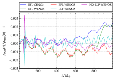
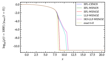
Figure 6: TOV star in a dynamical spacetime with $\Gamma$-law EoS. Top: Central rest-mass density evolution for simulations of a single spherical star with $n=96$ for different EFL reconstruction schemes. Bottom: One-dimensional rest-mass density profiles in the $x$-direction at time $t=1000$ with $n=96$. The profiles in the y- and z-direction are identical.

Another very interesting feature of the EFL method, that was also stressed in Guercilena et al. (2017), is the behaviour of the entropy production profile with increasing resolution. The bottom panel of Fig. 5 shows this behaviour: with increasing resolution the entropy production function’s peaks sharpen and are better localised around the surface of the star. This shows that the EFL method is able to adjust the entropy production function $\nu$ according to the size of the grid-cells. The finer they become, the more accurate the problematic regions are flagged by the entropy. Ideally, the entropy production profile will tend to a delta function located around the surface of the star at infinite resolution.

Having secured the proper flagging of the problematic regions and the correct implementation of the EFL method, we check further its performance during the evolution of the TOV star by monitoring the dynamical behaviour of the central rest-mass density. The oscillation of the central rest-mass density $\rho_{\rm max}$ of the EFL method with different reconstruction schemes is presented, together with the LLF-WENOZ and HO-LLF-WENOZ methods Bernuzzi and Dietrich (2016), on the top panel of Fig. 6. The performance (i.e. the amplitude of the oscillations) of the EFL method is comparable to the LLF-WENOZ and HO-LLF-WENOZ schemes and to the corresponding results of Fig. 12 in Guercilena et al. (2017).

In the bottom panel of Fig. 6 the profile of the rest-mass density relative to its initial maximum value $\rho_{\rm max}$ along the $x$-direction is depicted. (The profiles along the $y$- and $z$-direction are, as expected from the spherical symmetry of the TOV star, identical.) It is evident that the EFL method manages to capture the sharp transition between the interior of the TOV star and the outside vacuum better than the LLF-WENOZ and HO-LLF-WENOZ schemes. It has been also observed that the EFL profiles converge to the exact profile with increasing resolution. Comparing now our results with the corresponding ones of Fig. 11 in Guercilena et al. (2017), one can readily conclude that the EFL method does not experience the direction dependent oscillations reported in Guercilena et al. (2017) in any direction, including the diagonal.

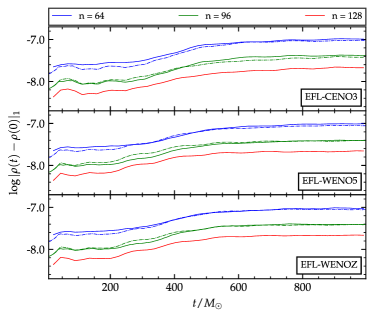
Figure 7: Evolution of the $L_{1}$-distance $||\rho(t)-\rho(0)||_{1}$ for a static TOV star in a dynamically evolved spacetime with a $\Gamma$-law EoS. All three EFL reconstruction schemes are presented. Dashed lines show results scaled to second-order.

The static character of the TOV star enables us to check the convergence properties of the EFL method as the exact solution can be read off from the initial data. Here we consider the $L_{1}$-norm of the difference between the three-dimensional evolution profile of the rest-mass density and the corresponding exact solution (initial data) and study its behaviour with time. The $L_{1}$-distance from the exact solution for the three reconstruction schemes used here are depicted in Fig. 7. The convergence rate of all the schemes considered is approximately second order in agreement with the result of Bernuzzi and Dietrich (2016) and the fact that the error at the stellar surface dominates the evolution. Notice though that, for the same resolution, the absolute errors of the EFL method are in average 100 times smaller than the ones observed in Bernuzzi and Dietrich (2016).

IV.2 Rotating neutron star

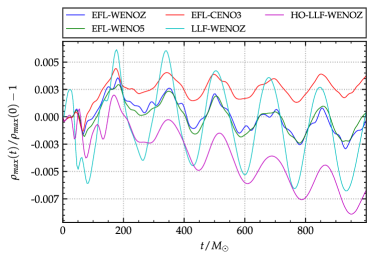
Figure 8: Central rest-mass density evolution for simulations of a stationary RNS in a dynamical spacetime with $\Gamma$-law EoS and $n=96$. Different EFL reconstruction schemes are shown.

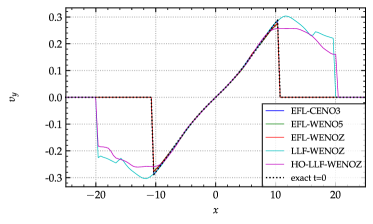
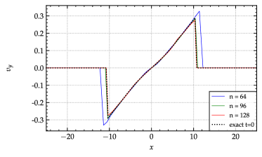
Figure 9: Velocity profile of a stationary rotating neutron star in a dynamical spacetime with $\Gamma$-law EoS. Top: One-dimensional profile of the velocity component $\upsilon_{y}$ along the $x$-direction at time $t=1000$ (four periods) with $n=128$. Bottom: The $\upsilon_{y}$ profile of the WENO5 scheme with increasing resolution.

We proceed now to the study of stationary neutron stars. The Rotating Neutron Star (RNS) code Stergioulas and Friedman (1995); Nozawa et al. (1998) is utilised to construct initial data for a stable uniformly rotating neutron star of central rest-mass density $\rho_{c}=1.28\times 10^{-3}$, axes ratio 0.65 and gravitational mass $M=1.666M_{\odot}$ described by a polytropic EoS with $\Gamma=2$. This is the BU7 model described in Dimmelmeier et al. (2006).

The star is evolved with the $\Gamma$-law EoS and the metric components with the Z4c scheme. The spacetime is dynamically evolved.

We start by checking the behaviour of the central rest-mass density with time. Fig. 8 presents the evolution of the central rest-mass density for the EFL method (with three different reconstruction schemes) and compares to the LLF-WENOZ and HO-LLF-WENOZ methods Bernuzzi and Dietrich (2016). The resulting oscillating behaviour is triggered by atmosphere effects and converges to 0 with increasing resolution. The results of all three methods are comparable with the oscillatory behaviour of the EFL method to be the smallest.

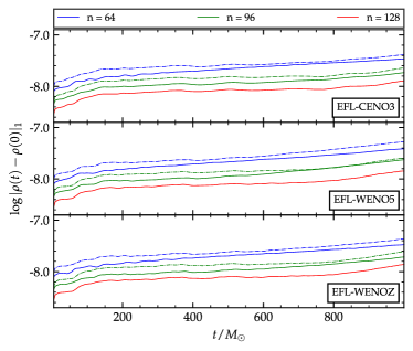
Figure 10: Evolution of the $L_{1}$-distance $||\rho(t)-\rho(0)||_{1}$ for a rotating neutron star in a dynamically evolved spacetime with $\Gamma$-law EoS. Dashed lines show results scaled to second-order.

For uniformly rotating neutron stars one expects that the velocity increases linearly with the distance from the centre of the star, reaches its maximum value at the surface and drops to zero from there on. The top panel of Fig. 9 shows the velocity component $\upsilon_{y}$ along the $x$-axis after four rotational periods (4P). The results for the EFL method (with three different reconstruction schemes) are presented and compared to the LLF-WENOZ and HO-LLF-WENOZ methods. It is apparent that the EFL method is superior in preserving the original velocity profile of the star (with the CENO3 scheme capturing the initial profile exactly). Comparing our results with the ones that can be found in the literature Font et al. (2002); Stergioulas and Font (2001); Font et al. (2000), we observe that the EFL method can capture better the rapid transition from the maximum value of the velocity at the surface of the star to zero just outside it. At the bottom panel of Fig. 9 the profile of $\upsilon_{y}$ for the WENO5 scheme is presented with increasing resolution—the other two reconstruction schemes show similar behaviour. The numerical solutions converge to the initial exact velocity profile with increasing resolution. The above results clearly demonstrate the ability of the EFL method to maintain the initial stationary equilibrium configuration during the evolution.

Finally, we check the convergence properties of the $L_{1}$-distance of $\rho(t)$ from the exact solution $\rho(0)$. Fig. 10 depicts the time-evolution of the $L_{1}$-norm of the difference between the three-dimensional profile of the rest-mass density and its initial profile for the three reconstruction schemes used here. All schemes show approximately second-order convergence.

V Binary neutron star evolutions

V.1 Initial data and numerical setup

Having thoroughly tested the EFL method with several special relativistic and single NS configurations, we move to discuss the EFL method in general relativistic simulations of neutron star binaries. In the following, we study the dynamics of two specific BNS configurations: BAM:100 and BAM:97, see Dietrich et al. (2018c). We chose these two BNS simulations because they enable us to study the performance of the EFL method in a short (BAM:100) and a long (BAM:97) BNS dynamical evolution. The neutron stars merge after approximately 3 revolutions for BAM:100 and after 10 for BAM:97. In addition, both simulations were already extensively studied in the literature, see Bernuzzi and Dietrich (2016), to which we refer and compare our results with. In subsection V.2 yet another three-orbit simulation, BAM:27, is used in order the test the EFL method with a different EoS. Although, our results for BAM:27 are consistent with the ones presented here, in the following, for the sake of presentational clarity, we do not discuss BAM:27 but focus on the other two simulations of Tab. 3.

Table 3: BNS quasicircular initial data. Columns: name, EoS, number of orbits, binary mass $M$, rest-mass $M_{b}$, ADM mass $M_{\mathrm{ADM}}$, angular momentum $J_{0}$, GW frequency $2M\Omega_{0}$. All configurations are equal-masses and irrotational.

Name	ID	EoS	orbits	$M$	$M_{b}$	$M_{\mathrm{ADM}}$	$J_{0}$	$2M\Omega_{0}$
BAM:100	Lorene	SLy	3	2.700	2.989	2.671	6.872	0.060
BAM:27	Lorene	$\Gamma=2$	3	3.030	3.250	2.998	8.835	0.055
BAM:97	Lorene	SLy	10	2.700	2.989	2.678	7.658	0.038

Table 4: Grid configurations of BNS simulations. Columns (left to right): name of BNS simulation, $L$: refinement levels, $l^{\mathrm{mv}}$: minimum moving level index, $n^{\mathrm{fix}}$: number of points per direction in fixed levels, $n$: number of points per direction in moving levels, $h_{L-1}$: resolution per direction in the finest level $l=L-1$, $h_{0}$: resolution per direction in the coarsest level $l=0$.

Name	$L$	$l^{\mathrm{mv}}$	$n^{\mathrm{fix}}$	$n$	$h_{L-1}$	$h_{0}$
BAM:100	7	2	128	64	0.228	14.592
	7	2	192	96	0.152	9.728
	7	2	256	128	0.114	7.296
	7	2	320	160	0.0912	5.8368
BAM:97	7	2	160	64	0.228	14.592
	7	2	240	96	0.152	9.728
	7	2	320	128	0.114	7.296
	7	2	400	160	0.0912	5.8368
BAM:27	7	1	96	64	0.312	20.0

The initial data that we evolved can be found in Tab. 3. They are conformally flat irrotational BNS configurations in quasicircular orbits computed with the Lorene library Gourgoulhon et al. (2001) and characterised by the Arnowitt-Deser-Misner (ADM) mass-energy $M_{\rm ADM}$, the angular momentum $J_{0}$, the baryonic mass $M_{b}$ and the dimensionless GW circular frequency $M\omega_{0}$.

The initial data for BAM:100 and BAM:97 were evolved with the EFL method in 16 different resolution and reconstruction combinations. BAM:100 was evolved with the CENO3, WENO5 and WENOZ reconstructions. For each reconstruction four different grid resolutions were considered. The grid specifications for all the runs are reported in Tab. 4. BAM:97 was evolved only with the WENOZ reconstruction scheme. The reason for this is, as it will become apparent in the following, that the BAM:100 results strongly indicate that the best performing reconstruction scheme is WENOZ. The atmosphere setting for both simulations are $f_{\rm atm}=10^{-11}$ and $f_{\rm thr}=10^{2}$. The metric is evolved with the Z4c scheme. Standard radiative boundary conditions are used for all BNS simulations.

V.2 Qualitative behaviour of the entropy production

The most basic and simple check of the EFL method is to inspect if the produced NS trajectories agree with the ones in the literature Bernuzzi and Dietrich (2016). Fig. 11 depicts the behaviour with time of the proper distance between the NSs of the ten-orbit BAM:97 simulation for the EFL-WENOZ and HO-LLF-WENOZ schemes at different resolutions. The time of merger can be determined from the vanishing of the proper distance. Notice that while for high resolutions the two methods agree, for low resolutions their behaviour differs as shorter inspirals are expected for lower resolutions because of numerical dissipation Bernuzzi et al. (2012b, a). It is evident from Fig. 11 that although the trajectories of the HO-LLF-WENOZ scheme for low resolutions are less accurate than the ones of the EFL-WENOZ scheme, they catch up with increasing resolution. Thus, one would expect that the trajectories of the HO-LLF-WENOZ scheme converge faster to the actual trajectory of the inspiraling NSs. Indeed, by conducting self-convergence tests for the triplets $n=(64,96,128)$ and $n=(96,128,160)$ we conclude that the actual convergence rate of the proper distance for the EFL-WENOZ scheme is approximately third- and fourth-order, respectively. A similar analysis for the HO-LLF-WENOZ scheme shows that the convergence rates for the above triplets are approximately fourth- and six-order, respectively. The trajectories of the three-orbit BAM:100 simulation show similar behaviour.

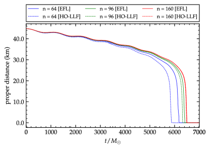
Figure 11: Time evolution of the proper distance between the NSs for the ten-orbit BAM:97 simulation. Different grid resolutions are presented for the EFL-WENOZ method (solid lines) and HO-LLF-WENOZ method (dashed lines).

The entropy production function $\nu$ plays a central role in our method. Hence, it is of great interest to study its behaviour during the evolution of BNS merger simulations. In the following, we discuss the two-dimensional entropy production profiles of two different three-orbit simulations. Together with the three-orbit BAM:100 simulation, we present here another three-orbit simulation with a different EoS. The reason for this is to exemplify the dependence of our method on the EoS used, which is best depicted by the entropy production profile. We use the BAM:27 simulation Dietrich et al. (2018c) with initial data parameters given in Tab. 3.

In Fig. 13 and Fig. 13 we present two-dimensional hybrid plots depicting the entropy production function $\nu$ and rest-mass density $\rho$ profiles at different stages of a $\Gamma$-law (BAM:27) and SLy (BAM:100) simulation, respectively. The different panels show (from left to right) selected snapshots of the inspiral, merger and post-merger stages, respectively. We first notice that the SLy simulation displays considerably more features in both $\nu$ and $\rho$ profiles compared to the $\Gamma$-law simulation. Taking a closer look at the $\nu$ profile, we see that during the $\Gamma$-law simulation the EFL is only activated at the surface of each NS. The same can be also observed in the SLy simulation, however, here also regions in exterior of the NSs are flagged for limiting. Judging from the corresponding rest-mass density plots, the flagging in the exterior is due to the SLy simulation carrying a matter cloud around the stars, a feature that is absent from the $\Gamma$-law simulation.

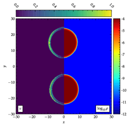
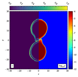
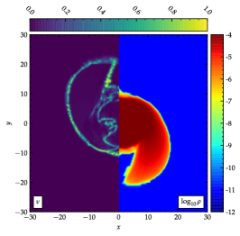
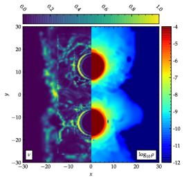
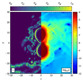
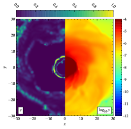
Figure 12: Two-dimensional hybrid plots depicting the entropy production and rest-mass density profiles across different stages of the BAM:27 simulation. Notice that BAM:27 uses a $\Gamma$-law EoS. Left to right: inspiral, merger, post-merger.

Figure 13: Two-dimensional hybrid plots depicting the entropy production and rest-mass density profiles across different stages of the BAM:100 simulation. Notice that BAM:100 uses a SLy EoS. Left to right: inspiral, merger, post-merger.

During the inspiral phase of Fig. 13 we can see that there are actually two concentric layers where the EFL is activated around the surface (left panels). When the stars first touch, their interior and exterior layers start merging with each other (middle panels). After the first contact the inner layer also starts moving inwards before it becomes again concentric with the surface layer (right panels). The surface layer continues tracking the star’s surface during merger which is evident by its alignment with the matter-vacuum interface that can be seen in the rest-mass density profile. It seems that this double-layer formation is universal, because we find similar behaviour during the RNS evolutions. Interestingly, the mass density plots do not show apparent features that would need shock treatment in the region where the second layer appears. There are two reasons causing this double-layering: i) Low resolution: With increasing resolution the entropy production function $\nu$ gets better localised around the surface of the NSs, see bottom panel of Fig. 5, and consequently the amplitude of the inner peak of $\nu$ decreases; ii) The entropy production function $\nu$ is overproduced by setting $c_{E}=1$ in (14). Recall that for the sake for generality and simplicity we set $c_{E}=1$ in all our simulations. By choosing a smaller value for the tunable constant $c_{E}$, the values of $\nu$ would scale down accordingly. The inner layer then would reduce. While it is possible to experiment with the values of $c_{E}$ to minimize this effect, we find that the convergence properties of the solutions are not affected by it.

Lastly, the same double layer formation can also be observed in Fig. 13, although the amplitude of the inner layer is smaller and the exterior layer appears to be wider.

V.3 Conserved quantities

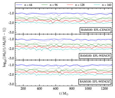
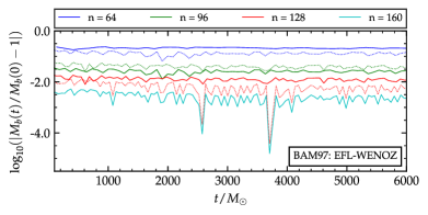
Figure 14: Conservation and convergence of the total rest-mass on the refinement level $l=2$. Top: Three-orbit BAM:100 simulation. All three reconstruction schemes are presented for different grid resolutions. Dotted lines show results scaled to third-order. Bottom: Ten-orbit BAM:97 simulation. The WENOZ reconstruction schemes is presented for different grid resolutions. Dotted lines show results scaled to fourth-order.

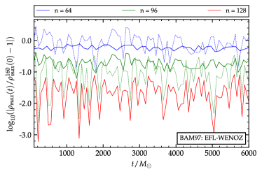
Figure 15: Evolution and convergence of the central rest-mass density on the refinement level $l=1$ for the ten-orbit BAM:97 simulation. Dotted lines show results scaled to fifth-order.

Conserved quantities can be used as quantitative and qualitative diagnostics of the performance of a numerical scheme. Therefore, before discussing the waveform accuracy of our simulations, we study the convergence properties of these quantities. During the BNS evolution we monitor:

• The total rest-mass of the matter, $M_{b}=\int d^{3}x\sqrt{\gamma}\,D$, where the integral is performed over the whole computational domain. The continuity equation (1) guarantees that the total rest-mass should be conserved in the absence of a net influx or outflow of matter. We use a conservative numerical scheme (2), which is expected to preserve the rest-mass to its initial value. This requirement is trivially satisfied on a single grid, but violations are generically expected in the presence of the artificial atmosphere and when adaptive mesh refinement is used, see e.g. Dietrich et al. (2015b).

• The dynamical behaviour of the central rest-mass density, $\rho_{\rm max}(t)$, of the NSs. Unlike the stationary single star simulations, this quantity is not exactly conserved in BNS simulations because of the presence of tidal interactions. However, during the early orbits of the inspiral, tidal interactions are weak and contribute only small oscillations around the initial value. For the considered resolutions, the latter are actually smaller than the oscillations induced by truncation errors and should converge to zero with increasing resolution. Hence, the ratio of the central rest-mass density to its initial value for the highest resolution, i.e. the quantity $\rho_{\rm max}(t)/\rho^{n_{\rm max}}_{\rm max}(0)$, should tend to one with increasing resolution.

• The $L_{2}$ norm of the Hamiltonian constraint. It is expected that in the continuum limit it vanishes, thus the Hamiltonian constraint of any numerical solution must convergence to zero in order to be consistent with Einstein’s equations.

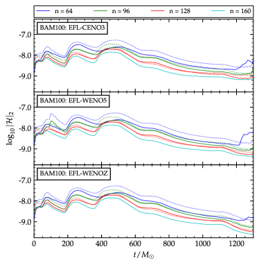
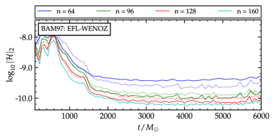
Figure 16: $L_{2}$ norm of the Hamiltonian constraint on the refinement level $l=1$ for the BNS simulations. Top: Three-orbit BAM:100 simulation. All three reconstruction schemes are shown. Bottom: Ten-orbit BAM:97 simulation. Dotted lines show results scaled to second-order.

Fig. 14 depicts the violation of the total rest-mass conservation during the inspiral and up to merger for the BNS simulations considered here. On the top panel the results for the three-orbit BAM:100 simulation are shown. Each sub-panel depicts one of the reconstruction schemes used here for four different resolutions. The violation of the rest-mass conservation during the inspiral phase is mainly caused due to artificial atmosphere treatment and mesh refinement boundaries. According to Fig. 14, during the evolution the mass violation shows small oscillations around its initial value, but is neither increasing nor decreasing. The mass violation converges to zero in an approximately third-order convergence pattern with increasing resolution. (Dotted lines show results scaled to third-order.) After the merger mass loss is caused by the ejected material which decompresses while it leaves the central region of the numerical domain (not shown in the plot). The performance of all three reconstruction schemes is comparable. In the bottom panel the respective mass violation for the BAM:97 simulation with the WENOZ scheme is presented. The behaviour of the mass violation of BAM:97 is quantitatively similar to the BAM:100 simulation, although BAM:97 converges with fourth-order and the absolute mass violation is smaller at the highest resolution.

The evolution of the central rest-mass density together with its convergence pattern on the $l=1$ refinement level for the ten-orbit BAM:97 simulation are presented in Fig. 15. The relative error $\rho_{max}(t)/\rho^{160}_{max}(0)$ is used to monitor the central rest-mass density during the evolution, where $\rho^{160}_{max}(0)$ is the initial value of the central rest-mass density for the highest resolution $n=160$ used here. It is evident from Fig. 15 that the residual $|\rho_{max}(t)/\rho^{160}_{max}(0)-1|$ with increasing resolution tends to zero with an approximate fifth-order convergence rate. Notice that the observed oscillatory behaviour gradually dies out with increasing resolution, but because of the logarithmic scale of Fig. 15 this feature is not easily seen.

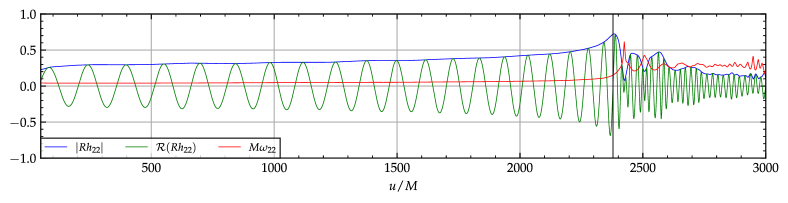
Figure 17: Amplitude (blue) and real part (green) of strain $Rh_{22}$ as well as instantaneous frequency $M\omega_{22}$ (red) of the GW signal obtained from the ten-orbit BAM:97 simulation using the EFL-WENOZ scheme. The time of merger is defined as the first peak in the amplitude $A_{22}$ and is indicated by a black vertical line at $u_{\rm mrg}\approx 2400M$.

The $L_{2}$ norm of the Hamiltonian constraint on refinement level $l=1$ up to merger with increasing resolution for both BNS simulations is presented in Fig. 16. In the top panel results for all three reconstruction schemes used in the BAM:100 simulations are presented for four different resolutions. In all cases the violation of the constraint is of the order of $\sim 10^{-8}$ for the lowest resolution of 64 points and decreases to zero with increasing resolution. The observed convergence is approximately second-order and agrees with the corresponding results in Bernuzzi and Dietrich (2016). (Dotted lines show results scaled to second-order convergence.) We attribute this behaviour to the to the constraint propagation and damping properties of the Z4c evolution system Weyhausen et al. (2012). Notice that in all cases during the evolution the constraint violation remains below its initial value and only increases, as expected, close to merger. Moreover, the Hamiltonian violation and convergence is similar in all the AMR levels independently on the fact that the matter is well resolved or not on the grid. This suggests that truncation error from AMR boundaries, boundary conditions and Berger-Oliger time interpolation are likely dominant in this quantity for Z4c. The performance of all reconstruction schemes is comparable, with the WENOZ scheme showing smaller constraint violation for the same resolution than the other two schemes. In the bottom panel results for the ten-orbit BAM:97 simulation are shown with the WENOZ scheme. The behaviour of the constraint violation is similar to the one observed for the BAM:100 simulation, with the slight difference that now the plots are a bit less smooth and that the constraint violation is smaller for the same resolution.

This second-order convergence of the violation of the Hamiltonian constraint is in stark contrast with the observed fourth-order or higher convergence of i) the rest conserved quantities studied in the present section, ii) the proper distance, see subsection V.2 and iii) the GW phase differences, see Fig. 19. Second-order convergence in the violation of the Hamiltonian constraint has been observed in all the BNS simulations produced with BAM to date, see Bernuzzi et al. (2012b); Thierfelder et al. (2011); Hilditch et al. (2013); Bernuzzi and Dietrich (2016). In addition, the results of Fig. 16 are similar to the corresponding ones in Bernuzzi and Dietrich (2016). The lower convergence rate in the Hamiltonian constraint violation is due to the details of BAM’s infrastructure, and not to the EFL itself. The main reasons are i) the fact that for efficiency the primitives are not synchronised in BAM and consequently the Hamiltonian is computed from the rest-mass density $\rho$ from a half time-step before ii) the propagation properties of Z4c, which means that an error contribution also comes from the boundary/AMR interpolation.

V.4 Gravitational wave analysis

We discuss here the impact of the EFL scheme on the gravitational waveforms. We follow closely Bernuzzi and Dietrich (2016) and examine the phase convergence in the inspiral-merger GWs and the associated error budget.

GWs are computed from the curvature scalar field $\Psi_{4}$ on coordinate spheres that are a distance $r$ from the origin of the computational domain. GW reconstruction is done by expanding $\Psi_{4}$ into spin weighted spherical harmonics to obtain the modes $\psi_{\ell m}$ and then solving $\ddot{h}_{\ell m}=\psi_{\ell m}$ using fixed frequency integration (FFI) Reisswig and Pollney (2011). We represent this complex valued field in polar representation as

$$Rh_{\ell m}=A_{\ell m}e^{-i\phi_{\ell m}},$$ (21)

where $A_{\ell m},\phi_{\ell m}$ are the amplitude and phase, respectively. We plot all results against the retarded time coordinate

$$u=t-R_{\ast}=:t-R(r)-2M\log\left(\frac{R(r)}{2M}-1\right),$$ (22)

where $M$ is the total gravitational mass of the BNS system. $R(r)=r(1+M/2r)^{2}$ is the radius in Schwarzschild coordinates and $r$ corresponds to the radius in isotropic coordinates which we take to be the extraction radius of our simulation. The moment of merger $u_{\rm mrg}$ is estimated by looking at the dominant $(\ell,m)=(2,2)$ mode and the first peak of $A_{22}$ within the time frame where the merger is expected to occur.

The FFI applies a high-pass filter to remove non-linear drifts generated by noise in the time integrations of $\ddot{h}_{\ell m}=\psi_{\ell m}$. Such a filter is characterized by a cut-off frequency $\omega_{{\rm cut}\,\ell m}$ for each mode. We follow the suggestion made in Reisswig and Pollney (2011) to use $\omega_{{\rm cut}\,\ell m}=m\omega_{0}/2$, where $\omega_{0}=2\Omega_{0}$ is the GW frequency associated to the initial orbital angular frequency $\Omega_{0}$.

An example of a waveform obtained from the ten-orbit inspiral BAM:97 simulation using the EFL-WENOZ scheme is presented in Fig. 17. The wave train shows a first peak after around 21 cycles until merger near $u_{\rm mrg}=2400M$ where it is then followed up with a more complex structure that includes multiple peaks and a slow amplitude decay. We also plot the instantaneous GW frequency $\omega_{22}=-\mathcal{I}(\dot{h}_{22}/h_{22})$. It displays a drastic frequency increase near merger, which is a characteristic of a chirp-like signal.

We perform self-convergence studies based on simulations that use $(n_{i})=(64,96,128,160)$ points per direction on the highest refined AMR level, and name those resolutions as $(\textrm{LOW, MID, HIG, FIN})$. We analyse the phase differences

$$\Delta\phi^{(n_{i},n_{j})}_{\ell m}=\phi^{(n_{i})}_{\ell m}-\phi^{(n_{j})}_{\ell m}\,,$$ (23)

between pairs of resolutions. To determine the experimental convergence rate $p$ we rescale these differences by a factor $s$ that captures the rate by which we expect the differences to decrease with increasing resolutions, provided that our scheme converges. It is computed by Baumgarte and Shapiro (2010)

$$s(p,n_{i},n_{j},n_{k},n_{l}) =\frac{1-(n_{i}/n_{j})^{p}}{(n_{i}/n_{k})^{p}-(n_{i}/n_{l})^{p}},$$ (24)

where $n_{i}<n_{j}\leq n_{k}<n_{l}$.

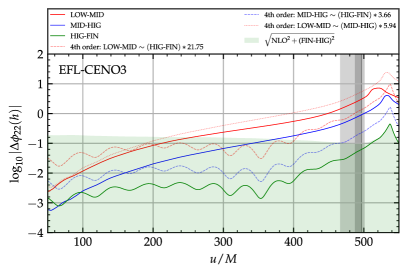
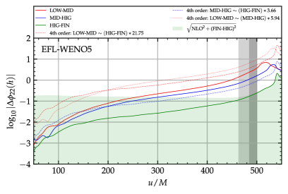
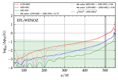
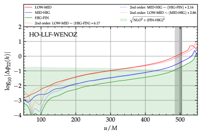
Figure 18: GW phase difference convergence rate study for the three-orbit BAM:100 simulation: Solid lines represent phase differences between runs with consecutively increasing resolutions; dashed and dotted lines correspond to rescaled differences of HIG-FIN and MIG-HIG differences, respectively, where the scaling factor is computed from (24) using an integer convergence rate $p$; the latter was determined experimentally by looking for the best visual overlap between dashed, dotted and solid lines of the same color (which we failed to do with the CENO3 and WENO5 reconstructions); the green shaded regions indicate the obtained error budget as discussed in the text; the gray shaded regions mark the differences in merger times between runs with consecutively increasing resolutions.

The error budget computation accounts for (i) finite radius extraction errors $\Delta\phi^{\rm rad}_{\ell m}$ and (ii) finite resolution errors $\Delta\phi^{\rm res}_{\ell m}$. Since they are of different origin and even come with a different sign Bernuzzi and Dietrich (2016) we compute the combined error using pointwise quadrature,

$$\Delta\phi^{\rm err}_{\ell m}=\sqrt{(\Delta\phi^{\rm rad}_{\ell m})^{2}+(\Delta\phi^{\rm res}_{\ell m})^{2}}.$$ (25)

The contribution (i) is estimated using the next-to-leading order (NLO) behaviour of $\Psi_{4}$ Lousto et al. (2010). The contribution (ii) is estimated as the phase difference between the two highest resolved runs, which we denote by (FIN-HIG). The rational behind this is that, for a convergent scheme, any result obtained with higher precision as those runs will give results below this difference.

V.4.1 Three-orbit BAM:100 simulation

Fig. 18 shows a self-convergence study of the waveform phase differences for the BAM:100 simulation. The first three panels correspond to the results obtained with the EFL and the reconstruction schemes CENO3, WENO5 and WENOZ, respectively. The fourth panel shows results obtained with the hybrid algorithm HO-LLF-WENOZ. This last result serves as a reference for a comparison with our EFL method.

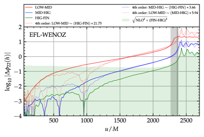
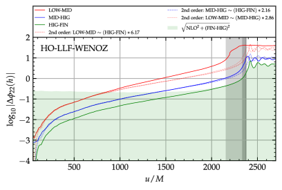
Figure 19: GW phase difference convergence rate study for ten-orbit BAM:97 simulation. Left panel: EFL-WENOZ method. Right panel: HO-LLF-WENOZ method.

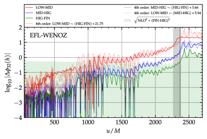
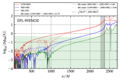
Figure 20: GW phase difference convergence rate study for higher modes for ten-orbit BAM:97 simulation using the entropy flux limiter with WENOZ reconstruction. Left panel: $(3,2)$ mode. Right panel: $(4,4)$ mode.

The first thing to note is that the phase differences between runs with consecutively increasing resolutions decrease for all simulations. This indicates that the scheme is capable of providing consistent results. This is further supported by the decrease in the difference between merger times, indicated by the narrowing of the gray shaded regions, which marks the difference between merger times of runs with consecutively increasing resolutions. Furthermore, all runs converge to a merger time near $u=500M$ independent of the method. The figure contains the combined phase errors (25) as green shaded areas. The estimated error of the highest resolved runs is ${\lesssim}0.1$ rad uniformly throughout the inspiral phase and to merger.

Focusing on the EFL results for CENO3 and WENO5, one can see that, although the phase differences decrease, it is not possible to assign a clear integer convergence rate $p$ for which the rescaled differences match with the true differences (at the simulated resolutions). By contrast, the plot demonstrates a clear fourth order ($p=4$) convergence with the WENOZ method (bottom left panel). For the CENO3 series (top left panel) we actually find a scaling consistent with $p=2$ for the differences LOW-MID and MID-HIG, but a higher scaling $p>2$ between the HIG-FIN difference. In the WENO5 series (top right panel) the convergence plot is strongly affected by the lowest resolutions, while the scaling seems to be closer to $p=4$ between the MID-HIG and HIGH-FIN resolutions. Also, the differences between resolutions for the WENO5 series are larger in absolute values than those of other methods. Overall, the difference between the CENO3, WENO5 and WENOZ series points to the importance of the choice of reconstruction in the LO flux in Eq. (8). In particular, the less dissipative and higher-resolution WENOZ scheme (vs. WENO5) Borges et al. (2008) is a confirmed key feature in BNS applications Bernuzzi et al. (2012a).

Comparing the EFL to the results obtained with the HO-LLF-WENOZ hybrid we find that the former shows a faster convergence rate for the EFL-WENOZ series and generically smaller absolute differences HIG-FIN at merger (except EFL-WENO5, see above). The HO-LLF-WENOZ algorithm (bottom right panel) yields a clean convergence pattern with $p=2$, consistent with previous results reported in Bernuzzi and Dietrich (2016), and phase differences FIN-HIG (errorbars) at merger a factor ${\sim}5$ larger than EFL-WENOZ.

V.4.2 Ten-orbit BAM:97 simulation

Fig. 19 shows a convergence study similar to Fig. 18 but based on results of the ten-orbit BAM:97 simulation. The simulations are performed with EFL-WENOZ and compared to those presented in Bernuzzi and Dietrich (2016) and obtained with the HO-LLF-WENOZ method.

For both methods phase differences consistently decrease by increasing the grid resolution. Both merger times tend to $u\approx 2400M$, thus indicating the results are consistent (cf. Fig. 11). Convergence can be demonstrated clearly in both cases. The EFL-WENOZ scheme produces a clear fourth order ($p=4$) convergent waveforms, consistent with the three-orbits simulations. Instead, the HO-LLF-WENOZ scheme produces second order convergent ($p=2$) results starting at MID resolutions; the convergence degrades for the LOW-MID difference towards the merger time Bernuzzi and Dietrich (2016). The phase differences FIN-HIG (errorbars) at merger for the HO-LLF-WENOZ are a factor ${\sim}3$ larger than for the EFL-WENOZ. In both cases they are a factor ${\sim}10$ larger than in the three-orbit runs (for comparable resolutions). We also note that the convergence rate is maintained in the early postmerger phase, suggesting that the EFL scheme is robust and can well capture the violent dynamics of the remnant NS.

Given this clear convergence pattern for the $(2,2)$ modes of the EFL-WENOZ runs, we also investigate the convergence of higher modes $h_{\ell m}$ with $\ell>2$. Fig. 20 shows a convergence study of the $(\ell,m)=(3,2),(4,4)$ modes. Also in this case, the phase differences show a consistent decrease with increasing resolution and a clear fourth-order convergence of the modes’ phase. The phase error is of order $10^{-1}$ rad, with a flat profile and rapidly accumulating only very close to the merger time. Furthermore, the convergence pattern continues to hold through merger. To our knowledge, this is the first time that a successful convergence study in higher modes of the GW strain is presented in the literature.

VI Waveforms’ Faithfulness

Table 5: Faithfulness functional $\mathcal{F}$ for the BNS simulation considered in the present work, see Tab. 3. The values of $\mathcal{F}$ are compared to the threshold values $\mathcal{F}_{\rm thr}$ calculated with (26) for different signal-to-noise ratios. The notation $\mathcal{F}_{\rm thr}^{\tilde{\rho},\epsilon}=1-\epsilon^{2}/2\,\tilde{\rho}^{2}$ has been introduced for the various threshold values, which are explicitly presented on the second row inside the brackets. A tick ✓  indicates that $\mathcal{F}>\mathcal{F}_{\rm thr}$ and a cross ✗  that $\mathcal{F}<\mathcal{F}_{\rm thr}$.

Simulation	Scheme	$n$	$\mathcal{F}$	$\mathcal{F}_{\rm thr}^{14,6}$	$\mathcal{F}_{\rm thr}^{14,1}$	$\mathcal{F}_{\rm thr}^{30,6}$	$\mathcal{F}_{\rm thr}^{30,1}$	$\mathcal{F}_{\rm thr}^{80,6}$	$\mathcal{F}_{\rm thr}^{80,1}$
				(0.9847)	(0.9974)	(0.9967)	(0.9994)	(0.9995)	(0.9999)
BAM:97	EFL-WENOZ	[160, 128]	0.9998	✓	✓	✓	✓	✓	✗
BAM:97	HO-LLF-WENOZ	[160, 128]	0.9992	✓	✓	✓	✗	✗	✗
BAM:100	EFL-CENO3	[160, 128]	0.9952	✓	✗	✗	✗	✗	✗
BAM:100	EFL-WENO5	[160, 128]	0.9991	✓	✓	✓	✗	✗	✗
BAM:100	EFL-WENOZ	[160, 128]	0.9987	✓	✓	✓	✗	✗	✗
BAM:100	HO-LLF-WENOZ	[160, 128]	0.9987	✓	✓	✓	✗	✗	✗

We check if the EFL numerical simulations are sufficiently accurate to produce faithful waveforms for gravitational-wave astronomy. We follow closely the methods and equations discussed in Damour et al. (2011); Gamba et al. (2021), to which we refer for a complete description. Previous results of this kind were presented in Bernuzzi et al. (2012b); Gamba et al. (2021).

The accuracy of numerical waveform for application to GW astronomy is often quantified in terms of the faithfulness functional $\mathcal{F}\in[0,1]$ by considering criteria in the form Gamba et al. (2021); Damour et al. (2011):

$$\mathcal{F}>\mathcal{F}_{\rm thr}=1-\frac{\epsilon^{2}}{2\,\tilde{\rho}^{2}},$$ (26)

with $\epsilon^{2}\leq 1$ and $\tilde{\rho}$ the signal-to-noise ration (SNR). Sometimes it is suggested Chatziioannou et al. (2017) to relax this criterion by taking $\epsilon^{2}=N$, where $N$ is the number of intrinsic parameters of the binary. The criterion $\mathcal{F}>\mathcal{F}_{\rm thr}$ is a necessary condition that has to be satisfied by faithful waveform models, i.e. suitable for GW parameter estimation. A possible violation of this criterion does not imply the presence of biases though. We compute threshold values $\mathcal{F}_{\rm thr}$ at SNRs $\tilde{\rho}=14$, $30$ and $80$ that correspond to the SNRs of GW190425, GW170817 and a generic loud signal, respectively. For each of these SNRs the values of $\mathcal{F}_{\rm thr}$ are evaluated for two different choices of $\epsilon^{2}$, i.e. $\epsilon^{2}=1$ and $\epsilon^{2}=N=6$. The faithfulness $\mathcal{F}$ is evaluated using the numerical waveforms at two different resolutions. The faithfulness integral is computed over a frequency range $f\in[f_{\rm low},f_{\rm mrg}]$, where $f_{\rm low}$ corresponds to the initial circular GW frequency of the simulation and $f_{\rm mrg}$ is the merger frequency. We employ the aLIGODesignSensitivityP1200087 Aasi et al. (2015) PSD from pycbc Nitz et al. (2020) to compute the matches. In order to obtain accurate mismatch results from numerical data, one has to pre-process the raw $\psi_{4,\rm lm}$ modes before performing the FFI method to obtain $h_{\rm lm}$. To this end we tapered the signals at the beginning and the end and also zero padded them for finer frequency bin resolution. The preprocessing should be done such that the instantaneous GW frequency $\omega_{22}$ computed from $h_{22}$ matches the GW frequency provided by the initial data, cf. table 3. We emphasize that this preprocessing step has no influence on the phase difference convergence rate.

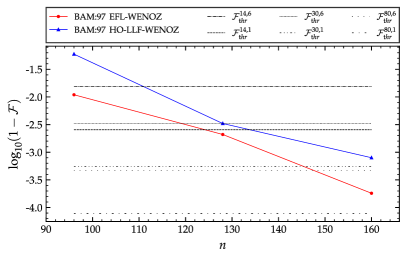
Figure 21: Faithfulness as a function of the resolution for the BAM:97 simulation.

Tab. 5 reports the faithfulness values for the $(2,2)$ waveforms of the BAM:97 and BAM:100 simulations. Each value of $\mathcal{F}$ is obtained from the two highest resolution simulations available, that represent a measure of the error as discussed above. All the waveforms, except for EFL-CENO3, produced with the EFL method pass the three lowest accuracy criterion of (26). The same holds for the corresponding waveforms computed with the HO-LLF-WENOZ method of Bernuzzi and Dietrich (2016). Out of the six simulations examined only the EFL-WENOZ for BAM:97 passes a higher accuracy test than the one with SNR $\tilde{\rho}=30$ and $\epsilon^{2}=6$. Actually, this specific simulation at resolution of $n=160$ passes five out of the six accuracy tests making it an ideal candidate for GW modeling studies. Note also that the faithfulness of BAM:100 with EFL-WENO5 is very close to pass the fourth accuracy test $\mathcal{F}_{\rm thr}^{30,1}=0.9994$.

In Fig. 21 we study the dependence of the faithfulness functional with simulation pairs of increasing resolution. Specifically, Fig. 21 shows the faithfulness between pairs of waveforms at different resolutions $n=[160,128],[128,96]$ and $[96,64]$ as a function of the resolution. The plot focuses on the longest BAM:97 simulation that is the most relevant for waveform modelling. It is apparent that for both schemes the quantity $1-\mathcal{F}$ converges, as expected, to zero with increasing resolution. Notice though that the EFL-WENOZ scheme produces more faithful waveforms than the HO-LLF-WENOZ scheme at the same resolution. With this convergence behaviour the EFL-WENOZ (HO-LLF-WENOZ) simulation is expected to pass the highest accuracy test $\mathcal{F}_{\rm thr}^{80,1}$ at resolution $n\sim 192$ ($n\sim 224$). The computational cost for a simulation at this resolution is approximately $\sim$1M CPU-hrs ($\sim$2.5M CPU-hrs).

VII Conclusions

This paper investigates, for the first time, the use of the EFL scheme, an entropy-based flux-limiter for the computation of the hydrodynamics’ numerical fluxes, in BNS merger simulations. The main question addressed here is whether the EFL is sufficiently robust for the treatment of the NS surface and smooth-flow regions to provide us with accurate and high-order converging gravitational waveforms. We answer this in the affirmative.

Our method builds on the proposal of Guercilena et al. (2017), but notably does not make use of a positivity preserving limiter nor of free-parameters (see subsection II.2). The new EFL scheme successfully passes a standard set of benchmark problems in special relativistic hydrodynamics, with results comparable to standard high-order characteristic WENO schemes, e.g. Bernuzzi and Dietrich (2016). Our scheme does not suffer from the oscillatory behaviour at the shock-tube discontinuities observed in the original implementation of Guercilena et al. (2017).

Next, our method is tested in Sec. IV against three-dimensional general-relativistic single NS configurations. The EFL scheme accurately locates the surface of stationary star solutions, see Fig. 5, and enables the use of the LO flux in this region while the interior remains mainly resolved by the HO flux. EFL simulations give results comparable to those obtained with standard WENO schemes Radice et al. (2014a); Bernuzzi and Dietrich (2016) and with the ELH Guercilena et al. (2017). However, our new simulations are free of the spurious direction-dependent effects found in Guercilena et al. (2017), see Fig. 6. In addition, the EFL scheme performs very well in the simulation of rapidly rotating stars. As shown by Fig. 9, the velocity profile and the sharp transition at the surface of the star are almost un-altered over four rotational periods and correctly converge to the exact (initial) solution. The results from both high-order WENO scheme or second-order finite-volume schemes with primitive reconstruction are significantly less accurate (at the same resolutions).

Finally, in Sec. V, the new entropy method is applied to BNS merger simulations. The EFL scheme can be used to successfully evolve binaries and the properties observed in single star tests carry over to the simulation with non-stationary spacetimes and neutron stars moving on the computational grid. As shown in Fig. 13 and Fig. 13, the entropy limiter locates the surface of the inspiraling NSs quite accurately and it converges to zero in regions of smooth flows. Further, it captures the collisional shocks at merger and the outward dynamics of spiral density waves, thus being robust also for postmerger evolutions.

A convergence study of the gravitational waveforms obtained from these simulations shows that the EFL with a low-order flux based on the WENOZ reconstruction (EFL-WENOZ) can deliver fourth-order convergent waveforms at current production resolutions (subsection V.4). Such a convergence is measured in the $(2,2)$ dominant mode of the strain but also in the next subdominant modes $(3,2)$ and $(4,4)$. To our knowledge, these are the first results in which fourth-order convergence is demonstrated. The estimated phase error in the EFL-WENOZ waveform is about a factor ${\sim}5$ smaller than the error in the state-of-the-art high-order WENOZ scheme used in the same BAM code, at the same resolution.

We conclude that our EFL scheme can be efficiently used for high-quality waveform production and for future large-scale investigations of the binary NS parameter space. These studies will aim at extending our previous investigation in both quality and simulation length Bernuzzi et al. (2012b, a, 2014); Dietrich et al. (2015b, a). The immediate target is to resolve tidal effects near the merger that are the main source of systematic error in current waveform approximations of GW astronomy Gamba et al. (2021). We estimate that this will require EFL-WENOZ multi-orbit and multi-resolution simulations resolving the NSs up to $n\sim 192$ grid points per direction. A ten-orbit convergent series is within reach of modern supercomputers (similar to those used for this work) at the approximate cost of ${\sim}$2M CPU-hrs.

In the postmerger regime, the EFL well tracks the front of the ejecta. From the right panels of Fig. 13 and Fig. 13 it is apparent that the EFL is triggered by the outward dynamics of the spiral density waves. The main source of inaccuracy of the ejecta is the progressively lower resolution of the low density material as it propagate outwards. There might be a benefit in using the high-order scheme of the EFL when ejecta starts to propagate but, most likely, the re-definement of the grid will become too severe at very large distances and it is likely the EFL performs similarly to other schemes. A detailed investigation of the benefits of the EFL for resolving the ejecta is left to further investigation.