Gravitational waves and mass ejecta from binary neutron star mergers: Effect of large eccentricities

Abstract

As current gravitational wave (GW) detectors increase in sensitivity, and particularly as new instruments are being planned, there is the possibility that ground-based GW detectors will observe GWs from highly eccentric neutron star binaries. We present the first detailed study of highly eccentric BNS systems with full (3+1)D numerical relativity simulations using consistent initial conditions, i.e., setups which are in agreement with the Einstein equations and with the equations of general relativistic hydrodynamics in equilibrium. Overall, our simulations cover two different equations of state (EOSs), two different spin configurations, and three to four different initial eccentricities for each pairing of EOS and spin. We extract from the simulated waveforms the frequency of the f-mode oscillations induced during close encounters before the merger of the two stars. The extracted frequency is in good agreement with f-mode oscillations of individual stars for the irrotational cases, which allows an independent measure of the supranuclear equation of state not accessible for binaries on quasicircular orbits. The energy stored in these $f$-mode oscillations can be as large as $10^{-3}M_{\odot}\sim 10^{51}$ erg, even with a soft EOS. In order to estimate the stored energy, we also examine the effects of mode mixing due to the stars’ offset from the origin on the $f$-mode contribution to the GW signal. While in general (eccentric) neutron star mergers produce bright electromagnetic counterparts, we find that for the considered cases with fixed initial separation the luminosity decreases when the eccentricity becomes too large, due to a decrease of the ejecta mass. Finally, the use of consistent initial configurations also allows us to produce high-quality waveforms for different eccentricities which can be used as a test bed for waveform model development of highly eccentric binary neutron star systems.

I Introduction

The detection of the binary black hole (BBH) merger GW150914 Abbott et al. (2016a) in 2015 has initiated the era of gravitational wave (GW) astronomy. Since then, a number of additional BBH systems have been detected Abbott et al. (2016b, c, 2017a, 2017b, 2017c). Apart from the detections of BBHs, the spectacular observation of both GWs and electromagnetic (EM) radiation from a binary neutron star (BNS) merger in August 2017, GW170817 Abbott et al. (2017d, e, f), has been a scientific breakthrough for multi-messenger astronomy. With the planned upgrades of the advanced GW detectors LIGO and VIRGO LIG ; Vir and the upcoming KAGRA KAG detector in Japan, the near future of GW astronomy is bright and multiple detections of compact binaries are expected in the coming years Abbott et al. (2018a, 2016d). In addition to those improvements, the possibility of a 3rd generation (3G) of GW detectors, such as the Einstein Telescope (ET) Hild et al. (2008); Punturo et al. (2010); Ballmer and Mandic (2015) and Cosmic Explorer Abbott et al. (2017g), is exciting, since 3G detectors are expected to be ten times more sensitive than currently operating detectors. 3G observatories would thus not only provide a significantly larger number of detections, but also give the possibility of detecting systems and signals not observable by current interferometers, e.g., the postmerger phase of the remnant formed after the collision Clark et al. (2014, 2016); Radice et al. (2016a, 2017); Abbott et al. (2017h) or highly eccentric BNS systems.

In fact, in anticipation of an increased number of BNS detections with higher signal-to-noise ratio and the possibility to detect such extreme configurations as precessing BNSs, highly eccentric systems, or high-mass ratio mergers, it becomes even more important to model compact binary waveforms accurately to allow for a precise measurement of the source parameters. In order to extract information from a measured GW signal, the data are compared with fast-to-evaluate waveform models, which need to cover the entire BNS parameter space to allow for the accurate estimation of the binary parameters for all possible systems. While there has been progress in improving waveform models for (moderately) eccentric BBH systems Hinderer and Babak (2017); Cao and Han (2017); Hinder et al. (2018); Huerta et al. (2018) and very recently Ref. Yang et al. (2018) proposed a series of studies for waveform model development which will capture the dynamics of BNS systems on eccentric orbits up to the merger of the stars, there is currently no waveform model for BNS systems on highly eccentric orbits. In numerical relativity (NR), most groups have focused on the simulations of quasi-circular BNS. This restriction is reasonable since the vast majority of systems are expected to have only a small eccentricity once the system enters the LIGO band due to the decay of eccentricity by the emission of gravitational radiation Peters (1964); Kowalska et al. (2011). However, different channels have been suggested for the formation of NS binaries that may retain non-negligible eccentricity when they merge.

One such proposed channel considers the capture of two initially mutually unbound neutron stars in a dense stellar system such as a nuclear star cluster via the emission of gravitational radiation during a close non-merging encounter Tsang (2013). Reference Tsang (2013) reports an estimate of the volume rate of such encounters of $\sim 0.003$–$6$ Gpc^-3 yr^-1. To obtain a possible detection rate, we need to incorporate the sensitive volume of ET. We assume two different scenarios to estimate the sensitive volume, which should bracket the sensitive volumes appropriate for realistic data analysis techniques (see, e.g., East et al. (2013) for initial work on such techniques). Specifically, we assume (i) the use of an unmodelled search for the kHz GW radiation emitted during the merger, for which one obtains a range of $\sim 20$ Mpc from Fig. 21 in Abernathy et al. , and (ii) that it is possible to construct a template bank of sufficiently accurate waveforms to enable a matched-filter search for these systems, giving a range of $\sim 8$ Gpc, where we estimate the range for highly eccentric binaries to be about half that for quasicircular binaries (obtained from Fig. 18 in Abernathy et al. ), since the matched filtering range for Advanced LIGO for highly eccentric binaries shown in Fig. 16 of East et al. (2013) is (on the larger side) about half that for quasicircular binaries quoted in Abbott et al. (2018a).

This leads to detection rates from this channel of the order of $10^{-7}$–$10^{-4}$ yr^-1 for burst searches [type (i)] and $10^{-1}$–$10^{3}$ yr^-1 for matched filter searches [type (ii)], where we computed the comoving volume within the range using Wright (2006).

Another dominant channel for eccentric BNS inspirals is suggested in Samsing et al. (2014), who consider binary-single star interactions in globular clusters (GCs) and find the rates to be $\sim 0.7$ Gpc^-3 yr^-1 for typical GCs containing $\sim 10^{3}$ NSs and assuming that 30% of these are in binaries. This would give eccentric BNS merger rates observable by ET on the order of $10^{-5}$ and $10^{2}$ yr^-1 for type (i) and (ii) searches, respectively. These numbers show that it might be possible to detect a few highly eccentric BNS mergers per year with an operating ET. We note that even if one is not able to perform a matched filter search, the unmodeled search numbers are surely pessimistic, as one should be able to do better than a purely unmodeled search for just the postmerger signal. Additionally, development of an eccentric BNS waveform model allowing for matched filtered searches would significantly boost the possibility of detecting highly eccentric BNS systems.

As eccentric BNSs merge, they may produce brighter EM emission than quasicircular mergers, making it important to understand such systems from a multimessenger perspective. Furthermore, the gravitational waveforms for highly eccentric binaries significantly differ from the classical chirp signal of quasicircular inspirals with its slowly increasing amplitude and frequency. On highly eccentric orbits, each encounter of the stars leads to a burst of GW radiation, first studied using Newtonian orbits together with leading order relativistic expressions for radiation and the evolution of orbital parameters Peters and Mathews (1963); Turner (1977a). Over the last decade, there have been numerical simulations of highly eccentric BBH Pretorius and Khurana (2007); Sperhake et al. (2008); Gold and Brügmann (2010, 2013) and BHNS Stephens et al. (2011); East et al. (2012a, 2015) systems in full general relativity (GR). There have been studies exploring highly eccentric (also known as dynamical capture) BNS in Newtonian gravity Lee et al. (2010); Rosswog et al. (2013) and in full GR simulations with approximate initial data (ID) using a simple superposition of two boosted NSs Gold et al. (2012); Radice et al. (2016b); Papenfort et al. (2018), and in East and Pretorius (2012); East et al. (2016a); Paschalidis et al. (2015); East et al. (2016b) with constraint solved ID, but not in hydrodynamical equilibrium.

Results for BHNS/BNS systems indicate a strong variability in properties of the wave and matter dynamics as a function of the eccentricity (or impact parameter). For example, for the eccentric BHNS systems studied in Stephens et al. (2011), the remnant disk masses range from nearly zero up to $\sim 0.3~{}M_{\odot}$, the unbound masses vary from zero to $\sim 0.15~{}M_{\odot}$ (computed from Table 1 of Stephens et al. (2011) using the baryonic mass of $1.49M_{\odot}$ from Table II of Read et al. (2009)). The energy and angular momentum emitted during the nonmerging first encounters are also found to vary by an order of magnitude depending on the impact parameter. The dynamical capture BNSs studied in Radice et al. (2016b) (the models labeled ‘HY_RPX’ in Table 1) also show variability in the type of merger remnant with impact parameter. Additionally, the unbound masses range from $\sim 0.0004$–$0.125~{}M_{\odot}$ as the impact parameter is varied, with corresponding variations in the signature of the electromagnetic counterparts.

An important result concerning BNS (or BHNS) is that eccentricity leads to tidal interactions that can excite oscillations of the stars, which in turn generate their own characteristic GW signal Turner (1977b); Kokkotas and Schäfer (1995); Chirenti et al. (2017); Parisi and Sturani (2018); Yang et al. (2018).

Neither the orbital nor stellar GWs have been studied so far for eccentric BNS orbits in GR with consistent ID, i.e., data which fulfill the Einstein constraint equations and the equations of general relativistic hydrodynamics in equilibrium, except for initial explorations with a simple equation of state in Moldenhauer et al. (2014), which still used an approximation for the velocity of the fluid, as opposed to solving for the velocity potential. The problems with using inconsistent ID are constraint violations, in cases for which the Einstein constraints are not fulfilled for the ID, or spurious matter density oscillations if the fluid is not in equilibrium. Those oscillations potentially spoil the quantitative analysis of matter oscillations which arise due to the encounters in eccentric BNSs.

Currently, there are a number of advanced solvers computing BNS initial data that are capable of exploring certain portions of the parameter space, e.g., the publicly available spectral code LORENE Bonazzola et al. (1999); Gourgoulhon et al. (2001, ), the Princeton group’s multigrid solver East et al. (2012b), BAM’s multigrid solver Moldenhauer et al. (2014), the COCAL code Tsokaros et al. (2015), SpEC’s pseudospectral solver Spells Foucart et al. (2008); Tacik et al. (2015), and the pseudospectral code SGRID Tichy (2009a, 2011, 2012); Dietrich et al. (2015a). Unfortunately, all of these solvers are incapable of reaching certain portions of the possible BNS parameter space. In particular, most of them cannot generate consistent initial data with specified high eccentricities. Only SGRID, the private LORENE version of Ref. Kyutoku et al. (2014), and the Spells code (cf. Tacik et al. (2015)) allow for adjusted orbital eccentricities for eccentric BNS simulations in a framework where the fluid equations are solved consistently..

In this paper we present the first detailed study of highly eccentric BNS systems using consistent ID extending the results of Dietrich et al. (2017a, b) in which we have already studied the effects of the mass ratio and spin. We consider equal-mass binaries at fixed initial separation ($\sim 165$ km) with two different EOSs and we vary the initial eccentricity. The chosen EOSs, SLy and MS1b, are reasonably representative of soft and stiff EOSs, respectively. Although analysis of the GW signal GW170817  Abbott et al. (2018b, c, 2017d) shows that MS1b predicts tidal deformabilities that are too large to agree with observation (since it gives stars that are not very compact), using this EOS allows us to understand the behavior of less compact stars.

The article is structured as follows: In Sec. II, we give a short description of the numerical methods and describe important quantities used to analyze our simulations. Section III summarizes the properties of the binaries we simulate. Section IV deals with the dynamics of the simulations, where in particular we focus on the conservative dynamics of the BNS system and the merger remnant. We discuss the properties of the dynamical ejecta and EM counterparts in Sec. V. In Sec. VI, we investigate the properties of the GW signal using spectrograms, and also consider the NS $f$-mode oscillations (including the effects of mode mixing due to the stars’ displacement from the origin and an estimate of the energy stored in these oscillations) and the postmerger GW frequencies. We conclude in Sec. VII. In Appendix A we test the accuracy of our simulations with respect to conserved quantities, the constraints and the waveforms.

Throughout this work we use geometric units, setting $c=G=M_{\odot}=1$, but occasionally give quantities in astrophysical units to allow for easier interpretation. Spatial indices are denoted by Latin letters running from 1 to 3 and Greek letters are used for spacetime indices running from 0 to 3.

All but two simulations we present here are already publicly available in the CoRe database of binary neutron star merger waveforms Dietrich et al. (2018); CoR . The remaining waveforms will be made available in the near future.

II Methods

II.1 Initial configurations

Our initial configurations are constructed with the pseudospectral SGRID code Tichy (2006, 2009a, 2009b); Dietrich et al. (2015a). SGRID uses the conformal thin sandwich formalism Wilson and Mathews (1995); Wilson et al. (1996); York Jr. (1999) in combination with the constant rotational velocity approach Tichy (2011, 2012) to construct quasiequilibrium configurations of spinning neutron stars and the methods presented in Moldenhauer et al. (2014); Dietrich et al. (2015a) to allow for eccentric BNSs. In particular we assume for each star in the eccentric BNS the approximate helliptical Killing vectors (where the name denotes a combination of helical and elliptical motion):

$$k_{1,2}^{\alpha}=t^{\alpha}+\Omega[(x-x_{c_{1,2}})y^{\alpha}-yx^{\alpha}]+\frac{v_{r}}{r_{12}}r^{\alpha}$$ (1a)

with

$$x_{c_{1,2}}=x_{\rm CM}+e(x_{1,2}-x_{\rm CM})$$ (1b)

the positions of the centers of the inscribed circles approximating the stars’ orbits. Here the stars (labeled by $1$ and $2$) start on the $x$-axis with positions $x_{1,2}$, $\mathbf{t}=\partial_{t}$, $\mathbf{x}=\partial_{x}$, $\mathbf{y}=\partial_{y}$ refer to the Cartesian coordinate vectors, $r^{\alpha}=(0,x,y,z)$ and $r_{12}=\left\lvert x_{1}-x_{2}\right\rvert$ is the distance between the star centers. The parameters $e$ and $v_{r}$ define the eccentricity and radial velocity, respectively—we take $v_{r}=0$ here. Additionally, $x_{\text{CM}}$ and $\Omega$ denote the system’s center-of-mass and angular velocity parameter, which are both determined by the force-balance equation, as discussed in Moldenhauer et al. (2014); Dietrich et al. (2015a), which give a more detailed discussion about the construction of eccentric BNS configurations.

SGRID’s computational domain is divided into six patches (Fig. 1 of Dietrich et al. (2015a)) including spatial infinity, which allows us to impose exact boundary conditions. We employ $n_{A}=n_{B}=28$, $n_{\varphi}=8$, $n_{\rm Cart}=24$ points for the spectral grid and give details of the configurations studied in Table 1.

II.2 Evolutions

Numerical relativity simulations are performed with the BAM code Brügmann et al. (2008); Thierfelder et al. (2011); Dietrich et al. (2015b); Bernuzzi and Dietrich (2016). The Einstein equations are written in 3+1 form using the BSSNOK evolution system Nakamura et al. (1987); Shibata and Nakamura (1995); Baumgarte and Shapiro (1998). The (1+log)-lapse and gamma-driver-shift conditions are employed for the evolutions Bona et al. (1996); Alcubierre et al. (2003); van Meter et al. (2006). The general relativistic hydrodynamics (GRHD) equations are solved in conservative form by defining Eulerian conservative variables from the rest-mass density $\rho$, pressure $p$, specific internal energy $\epsilon$, and 3-velocity, $v^{i}$. The system is closed by an EOS for which we use piecewise-polytropic fits of the SLy and MS1b EOSs; see Read et al. (2009). We include thermal effects by adding an additional thermal pressure of the form $p_{\rm th}=\rho\epsilon(\Gamma_{\text{th}}-1)$ with $\Gamma_{\rm th}=1.75$, cf. Bauswein et al. (2010).

The numerical domain is divided into a hierarchy of cell centered nested Cartesian grids. The hierarchy consists of $L$ levels of refinement labeled by $l=0$, $\cdots$, $L-1$. Each refinement level $l$ has one or more Cartesian grids with constant grid spacing $h_{l}$ and $n$ (or $n^{\rm mv}$) points per direction. The refinement factor is two such that $h_{l}=h_{0}/2^{l}$. The grids are properly nested, i.e., the coordinate extent of any grid at level $l$, $l>0$, is completely covered by the grids at level $l-1$. Some of the mesh refinement levels $l>l^{\rm mv}$ can be dynamically moved and adapted during the time evolution according to the technique of “moving boxes”; for this work we set $l^{\rm mv}=5$. The BAM grid setup considered in this work consists of nine refinement levels. Details about the different grid configurations employed in this work are given in Table 2; the grid configurations are labeled R1, R2, R3, R4, ordered by increasing resolution.

Time integration is performed with the method of lines using explicit fourth order Runge-Kutta integrators. Derivatives of metric fields are approximated by fourth-order finite differences, while a high-resolution-shock-capturing scheme based on primitive reconstruction and the local Lax-Friedrichs (LLF) central scheme for the numerical fluxes is adopted for the matter Thierfelder et al. (2011). Primitive reconstruction is performed with the fifth order WENOZ scheme of Borges et al. (2008).

Table 1: BNS configurations. The first column gives the configuration name and the second column gives the corresponding CoRe database ID. The next 5 columns provide the physical properties of the single stars: the EOS, the gravitational masses of the individual stars $M^{A,B}$, the baryonic masses of the individual stars $M_{b}^{A,B}$, the stars’ dimensionful and dimensionless spins $S^{A,B}$ and $\chi^{A,B}$. The last 5 columns give the input eccentricity $e$ [Eq. (1)], the 3PN eccentricity $\hat{e}_{\rm 3PN}$ [Eq. (11)], the initial GW frequency $M\omega^{0}_{22}$, the Arnowitt-Deser-Misner (ADM) mass $M_{\text{ADM}}$, and the ADM angular momentum $J_{\text{ADM}}$. The configurations evolved with different resolutions (cf. Table 2) are marked with asterisks (*).

Name	CoRe DB ID	EOS	$M^{A,B}$	$M^{A,B}_{b}$	$S^{A,B}$	$\chi^{A,B}$	$e$	$\hat{e}_{\rm 3PN}$	$M\omega^{0}_{22}$	$M_{\text{ADM}}$	$J_{\text{ADM}}$
SLy$-e0.40^{00}$	BAM:0112	SLy	$1.357558$	$1.504$	$0.0000$	$0.0000$	$0.40$	$0.52$	$0.0106$	$2.702935$	$8.8086$
SLy$-e0.45^{00*}$	BAM:0113	SLy	$1.357558$	$1.504$	$0.0000$	$0.0000$	$0.45$	$0.55$	$0.0110$	$2.702408$	$8.4514$
SLy$-e0.50^{00*}$	BAM:0114	SLy	$1.357558$	$1.504$	$0.0000$	$0.0000$	$0.50$	$0.60$	$0.0116$	$2.701945$	$8.0487$
SLy$-e0.60^{00}$	BAM:0115	SLy	$1.357558$	$1.504$	$0.0000$	$0.0000$	$0.60$	$0.69$	$0.0129$	$2.700947$	$7.1828$
SLy$-e0.40^{\uparrow\uparrow}$	BAM:0116	SLy	$1.358097$	$1.504$	$0.1767$	$0.0958$	$0.40$	$0.50$	$0.0107$	$2.703786$	$9.2346$
SLy$-e0.45^{\uparrow\uparrow*}$	BAM:0117	SLy	$1.358097$	$1.504$	$0.1767$	$0.0958$	$0.45$	$0.54$	$0.0111$	$2.703281$	$8.8478$
SLy$-e0.50^{\uparrow\uparrow}$	BAM:0118	SLy	$1.358097$	$1.504$	$0.1767$	$0.0958$	$0.50$	$0.59$	$0.0117$	$2.702773$	$8.4440$
SLy$-e0.60^{\uparrow\uparrow}$	BAM:0119	SLy	$1.358097$	$1.504$	$0.1767$	$0.0958$	$0.60$	$0.69$	$0.0130$	$2.701827$	$7.5714$
MS1b$-e0.45^{00}$	BAM:0074	MS1b	$1.380825$	$1.504$	$0.0000$	$0.0000$	$0.45$	$0.47$	$0.0119$	$2.748643$	$9.1766$
MS1b$-e0.50^{00}$	BAM:0075	MS1b	$1.380825$	$1.504$	$0.0000$	$0.0000$	$0.50$	$0.53$	$0.0125$	$2.748120$	$8.7322$
MS1b$-e0.60^{00}$	BAM:0076	MS1b	$1.380825$	$1.504$	$0.0000$	$0.0000$	$0.60$	$0.64$	$0.0139$	$2.747100$	$7.7936$
MS1b$-e0.45^{\uparrow\uparrow}$	BAM:0077	MS1b	$1.381270$	$1.504$	$0.2016$	$0.1056$	$0.45$	$0.48$	$0.0119$	$2.749629$	$9.5789$
MS1b$-e0.50^{\uparrow\uparrow}$	BAM:0078	MS1b	$1.381270$	$1.504$	$0.2016$	$0.1056$	$0.50$	$0.53$	$0.0125$	$2.749104$	$9.1487$
MS1b$-e0.60^{\uparrow\uparrow}$	BAM:0079	MS1b	$1.381270$	$1.504$	$0.2016$	$0.1056$	$0.60$	$0.64$	$0.0139$	$2.748047$	$8.2188$

Table 2: Grid configurations. The columns refer to: the resolution name, the number of points in the nonmoving boxes $n$, the number of points in the moving boxes $n^{\text{mv}}$, the grid spacing in the finest level $h_{8}$ covering the NS diameter, the grid spacing in the coarsest level $h_{0}$, and the outer boundary position $R_{0}$. The grid spacing and the outer boundary position are given in units of $M_{\odot}$

Name	$n$	$n^{\text{mv}}$	$h_{8}$	$h_{0}$	$R_{0}$
R1	$128$	$64$	$0.219$	$56.00$	$3612.000$
R2	$192$	$96$	$0.146$	$37.38$	$3606.784$
R3	$256$	$128$	$0.110$	$28.03$	$3602.112$
R4	$320$	$160$	$0.088$	$22.43$	$3599.309$

II.3 Simulation analysis

Most of our analysis tools were summarized in Refs. Dietrich et al. (2017a, b), including the computation of the ejecta properties, the disk masses, merger remnant characterizations, and the extraction of GWs.

Ejecta computation.

For the analysis in this paper, we extended our ejecta computation, which was previously purely based on the volume integration of the unbound matter, $M_{\rm ej}^{\mathcal{V}}$. Now, as an alternative method, we compute the matter flux of the unbound material across coordinate spheres sufficiently far from the system, $M_{\rm ej}^{\mathcal{S}}$; see e.g., Kastaun and Galeazzi (2015); Radice et al. (2016b). In general, we mark matter as unbound if it fulfills

$$u_{t}<-1\quad\text{and}\quad v^{i}x_{i}>0\ ,$$ (2)

where $u_{t}=-W(\alpha-\beta_{i}v^{i})$ is the time component of the fluid 4-velocity (with a lowered index), $\alpha$ is the lapse, $\beta^{i}$ is the shift vector, $W$ is the Lorentz factor, and $x^{i}=(x,y,z)$. For Eq. (2) we assume that the fluid elements follow geodesics and requires that the orbit is unbound and has an outward pointing velocity, cf. also East and Pretorius (2012). As pointed out in Dietrich et al. (2017a) a possible drawback is that material which gets ejected and decompresses can obtain densities of the order of the artificial atmosphere, which is added to allow stable GRHD simulations. Once the density drops below the atmosphere value material is not included in the ejecta computation anymore and the ejecta mass is possibly underestimated. For the case where we compute the ejecta mass due to the matter flux across a coordinate sphere this effect is reduced, since the decompression of material outside the coordinate sphere does not influence the ejecta mass computation. Specifically, based on the continuity equation and the Gauss theorem we compute the unbound mass as:

$$M_{\rm ej}^{\mathcal{S}}={\int_{0}}^{t}dt^{\prime}\int_{r=r_{\mathcal{S}}}[D_{u}\left(\alpha v^{i}+\beta^{i}\right)n_{i}]r^{2}d\Omega,$$ (3)

where $n_{i}=x_{i}/r$ with $r=\sqrt{x^{i}x_{i}}$. $D_{u}$ denotes the unbound fraction of conserved rest mass density $D=W\rho$. The estimates $M_{\rm ej}^{\mathcal{V}}$ and $M_{\rm ej}^{\mathcal{S}}$ are compared in Sec. V.1.

Spectrograms.

As discussed in the introduction, density oscillations can be induced in the stars during close encounters on highly eccentric orbits. Most of the oscillation energy is released in the f-modes which imprint their own characteristic GWs on top of the GWs generated by the orbital motion. In order to study these f-mode oscillations, we consider the spectrograms of the individual, $\ell=2$, dominant modes of the curvature scalar $r\Psi_{4}$.

We compute the frequency domain GW signal $r\tilde{\Psi}^{\ell m}_{4}(f)$ using the discrete Fourier transform implemented in MATLAB for time intervals of length $t_{2}-t_{1}$. The corresponding power spectral density (PSD) is given by

$$\operatorname{PSD}(r\Psi_{4}^{\ell m})(f)=(t_{2}-t_{1})^{2}\ \left\lvert r\tilde{\Psi}_{4}^{\ell m}(f)\right\rvert^{2}$$ (4)

to get the distribution of power into frequency components. This gives us a time series distribution of power and frequency, disentangling the dynamics of the system. From the spectrograms we find the frequency at which the NSs oscillate and also other frequencies of the dominant dynamics like inspiral, merger and the oscillations of the merger remnant. We also compute separate PSDs for the premerger and postmerger signal. These results will be discussed in more detail in Sec. VI.

Removing displacement-induced mode mixing from the GW signal:-

Since we are considering symmetric systems, the f-mode oscillations seen in the waveform will be twice those of an individual star. However, because the stars are not located at the origin, there will be some mode mixing which can not be neglected. Thus, it is not possible to simply divide the f-mode contribution to a given mode by $2$ to obtain the contribution from an individual star that would be extracted if it was at rest at the origin.

To obtain approximate expressions for an individual star’s multipole moments (as would be extracted with it at the origin), we will consider times when the stars are well-separated and approximately separate the f-mode signal from the signal from the orbit by taking a moving average of $\Psi^{4}_{2,\pm 2}$ with a window width given by the period of the $f$-mode. Specifically, we define $\Psi^{4,f\text{-mode}}_{2,\pm 2}:=\Psi^{4}_{2,\pm 2}-\Psi^{4,\text{avg}}_{2,\pm 2}$, where $\Psi^{4,\text{avg}}_{2,\pm 2}$ denotes the result of applying the moving average to $\Psi^{4}_{2,\pm 2}$.

Additionally, since the decay times of the $f$-mode oscillations are much longer than the time between periastra, one can treat the f-mode signal from a single star in a given $(\ell_{\text{i}},m_{\text{i}})$ mode as a simple sinusoid, $\Psi^{4,f\text{-mode}}_{\ell_{\text{i}},m_{\text{i}}}e^{i\omega_{f\text{-mode}}t}$, and can compute the mode mixing due to the stars’ displacement from the origin analytically using Eq. (43b) in Boyle (2016) (summing the series to obtain an exponential). This mode mixing is due to the variations in the retarded time at different points on the extraction sphere; we compute the retarded time approximately using the coordinate tracks of the stars. We thus take the retarded time to be $t_{\text{ret},0}+\alpha(\theta,\phi)$, where $t_{\text{ret},0}$ denotes the retarded time for a source at the origin, and $\alpha(\theta,\phi)=d_{1}\sin\theta\cos(\phi-\Upsilon)$ [cf. the discussion above Eq. (4) in Boyle (2016)]. Here $\theta,\phi$ are the angular spherical coordinates on the extraction surface and $d_{1}(\cos\Upsilon,\sin\Upsilon,0)$ is the coordinate track of star 1; the negative of this gives the track of the star’s companion. Additionally, we take each star to only have an intrinsic $(\ell_{\text{i}},m_{\text{i}})$ mode, since we can include further modes by linearity. Thus, the f-mode contribution to the (spin-weighted) spherical harmonic modes extracted from the evolution of the binary will be given by

$$\begin{split}\Psi^{4,\text{ext}}_{\ell,m}&=2\Psi^{4,f\text{-mode}}_{\ell_{\text{i}},m_{\text{i}}}\int_{S^{2}}\cos[d_{1}\omega_{f\text{-mode}}\sin\theta\cos(\phi-\Upsilon)]\\ &\quad\times{}_{-2}Y_{\ell_{\text{i}},m_{\text{i}}}(\theta,\phi){}_{-2}Y^{*}_{\ell,m}(\theta,\phi)d\Omega\\ &=:\mu_{\ell_{\text{i}},m_{\text{i}};\ell,m}\Psi^{4,f\text{-mode}}_{\ell_{\text{i}},m_{\text{i}}},\end{split}$$ (5)

where ${}_{-2}Y_{\ell m}$ is the spin-$(-2)$-weighted spherical harmonic, the star denotes the complex conjugate, and we have defined the mode mixing coefficient $\mu_{\ell_{\text{i}},m_{\text{i}};\ell,m}$, which describes mixing from the $(\ell_{\text{i}},m_{\text{i}})$ intrinsic mode of an individual star into the $(\ell,m)$ mode of the binary. Note that we have $\mu_{\ell_{\text{i}},m_{\text{i}};\ell,m}=\mu^{*}_{\ell,m;\ell_{\text{i}},m_{\text{i}}}$.

Defining $\zeta:=d_{1}\omega_{f\text{-mode}}$, we obtain mode mixing coefficients of

$$\mu_{2,\pm 2;2,\pm 2} =\frac{5}{8}\mathcal{S}(-3,-3;\zeta)$$

$$=2-\frac{5}{21}\zeta^{2}+O(\zeta^{4}),$$ (6a)

$$\mu_{2,0;2,0} =\frac{15}{4}\mathcal{S}(-3,1;\zeta)$$

$$=2-\frac{3}{7}\zeta^{2}+O(\zeta^{4}),$$ (6b)

$$\mu_{2,\pm 2;2,0} =\frac{5e^{\pm 2i\Upsilon}}{4}\sqrt{\frac{3}{2}}\mathcal{S}(5,1;\zeta)$$

$$=-\frac{2e^{\pm 2i\Upsilon}}{7\sqrt{6}}\zeta^{2}+O(\zeta^{4}),$$ (6c)

$$\mu_{2,\pm 2;2,\mp 2} =\frac{5e^{\pm 4i\Upsilon}}{8}\mathcal{S}(-35,5;\zeta)$$

$$=\frac{e^{\pm 4i\Upsilon}}{1512}\zeta^{4}+O(\zeta^{6}),$$ (6d)

where

$$\begin{split}\mathcal{S}(a,b;z)&:=\frac{z(3a+2bz^{2})\cos z+[-3a+(a-2b)z^{2}+z^{4}]\sin z}{z^{5}}\\ &\;=-a\frac{j_{2}(z)}{z^{2}}-2b\frac{j_{1}(z)}{z}+j_{0}(z)\end{split}$$ (7)

is a sinc-like function; we also give the expression in terms of the spherical Bessel functions of the first kind, $j_{\ell}$. We give the first few terms of the power series expansions to give intuition about the behavior of the mixing coefficients for small $\zeta$. We do not give the mixing coefficients involving the $(2,\pm 1)$ modes, as they vanish, due to the symmetry of the system (since we are assuming that the binary’s center-of-mass is at the origin in the current discussion). While the $\mu_{2,\pm 2;2,\mp 2}$ coefficients do not vanish, they are suppressed by higher powers of $\zeta$, only starting at $O(\zeta^{4})$, and are small enough for the situations we are considering (magnitudes $<0.03$) such that we will simply ignore them and focus on the much larger effects from the other mixing coefficients given above. Similarly, we do not consider mixing of higher-$\ell$ modes into the $\ell=2$ modes, since we expect those modes to have intrinsically smaller amplitudes, compared with the $\ell=2$ modes.

We also do not consider mode mixing due to the boosts, since the speeds due to the binary’s orbital motion are relatively small ($<0.15$) in the region between bursts, where the stars are well separated and the contributions from the mode mixing due to displacement from the origin are largest: The linear-in-velocity contribution to the mode mixing due to the boost vanishes, due to the symmetry of the binary (see Gualtieri et al. (2008) for explicit expressions in the linearized case; the general computation is discussed in Boyle (2016)).

If one needs to include the displacement of the binary’s center-of-mass from the origin, then it is simple to convert the expressions above to cover the general case: The contribution from a single star is just half of the total, so if the two stars are located at $d_{1}(\cos\Upsilon_{1},\sin\Upsilon_{1},0)$ and $-d_{2}(\cos\Upsilon_{2},\sin\Upsilon_{2},0)$, respectively, then, defining $\zeta_{A}:=d_{A}\omega_{f\text{-mode}}$ with $A\in\{1,2\}$, we have, e.g.,

$$\begin{split}\mu_{2,\pm 2;2,0}^{\text{general}}&=\frac{5}{8}\sqrt{\frac{3}{2}}\sum_{A=1}^{2}e^{\pm 2i\Upsilon_{A}}\mathcal{S}(5,1;\zeta_{A}).\end{split}$$ (8)

We use these general expressions for all the results presented in the paper, though the simpler expressions with the center-of-mass at the origin suffice in almost all cases. Additionally, for completeness, we also give the mixing from the intrinsic $(2,\pm 2)$ modes into the $(2,\pm 1)$ modes, though we do not consider these further in this paper:

$$\mu_{2,\pm 2;2,\pm 1}^{\text{general}} =\frac{5i}{8}\sum_{A=1}^{2}(-1)^{A}e^{\pm i\Upsilon_{A}}\mathcal{T}(3,1;\zeta_{A})$$

$$=\frac{i}{3}(\zeta_{1}e^{\pm i\Upsilon_{1}}-\zeta_{2}e^{\pm i\Upsilon_{2}})+O(\zeta_{1,2}^{3}),$$ (9a)

$$\mu_{2,\pm 2;2,\mp 1}^{\text{general}} =\frac{5i}{8}\sum_{A=1}^{2}(-1)^{A}e^{\pm 3i\Upsilon_{A}}\mathcal{T}(-5,-3;\zeta_{A})$$

$$=-\frac{i}{168}(\zeta_{1}^{3}e^{\pm 3i\Upsilon_{1}}-\zeta_{2}^{3}e^{\pm 3i\Upsilon_{2}})+O(\zeta_{1,2}^{5}),$$ (9b)

where

$$\begin{split}\mathcal{T}(a,b;z)&:=\frac{z(3a+z^{2})\cos z+(-3a+2bz^{2})\sin z}{z^{4}}\\ &\;=-3a\frac{j_{1}(z)}{z^{2}}+2b\frac{j_{0}(z)}{z}-y_{0}(z).\end{split}$$ (10)

Here $y_{\ell}$ are the spherical Bessel functions of the second kind. [Note that Mathematica (at least as of version 11) will not evaluate the $\theta$ integral giving the second of these mixing coefficients as is. However, if one uses the Maclaurin series for the Bessel function one obtains upon performing the $\phi$ integral first, and then integrates term-by-term, Mathematica will sum the resulting infinite series with no problems.]

III Configurations

In total, we consider $14$ different physical configurations, summarized in Table 1. All setups employ at least the R2 resolutions, cf. Table 2. A subset of configurations is also simulated with grid setups R1, R3, and R4. We mark those setups with an asterisks (^∗) in Table 1. The name of the simulations refer to: the EOS, the input eccentricity parameter used in Eq. (1), and the spin orientations. All results shown in the paper are obtained from the R2 resolution simulations, unless otherwise noted.

For this work we decided to focus on equal-mass setups with baryonic masses $M^{A}_{b}=M^{B}_{b}\simeq 1.504M_{\odot}$. The stars are either irrotational or have dimensionless spins of $\chi\simeq 0.1$ oriented parallel to the orbital angular momentum. To compute the rotation frequency of the stars corresponding to this dimensionless spin, we compared our results for the SLy EOS against rigidly rotating neutron stars computed with the publicly available Nrotstar module of the LORENE library Gourgoulhon et al. . Such a comparison is valid since rotating stars constructed employing the constant rotational velocity approach, as in SGRID Tichy (2011), have an almost zero shear Dietrich et al. (2015a); Tichy (2012). We obtain for the SLy setups a rotational frequency of $f\sim 191{\rm Hz}$.

In addition to the definition of eccentricity given in Sec. II.1 and the references there, we also compute the post-Newtonian (PN) eccentricity from the Arnowitt-Deser-Misner (ADM) expressions for the energy and angular momentum. In Dietrich et al. (2015a) an extensive comparison was performed between different order PN eccentricities and the eccentricity measure used in the helliptical symmetry vector in SGRID. Following this work, we use the 3PN expression for eccentricity, Eq. (4.8) in Dietrich et al. (2015a), computed following Mora and Will Mora and Will (2004). For completeness we also give the full expression below:

$$\begin{split}\hat{e}_{\rm 3PN}^{2}&=1-2\xi+\left[-4-2\nu+(-1+3\nu)\xi\right]E_{b}\\ &\quad+\left[\frac{20-23\nu}{\xi}-22+60\nu+3\nu^{2}-(31\nu+4\nu^{2})\xi\right]E_{b}^{2}\\ &\quad+\left[\frac{-2016+(5644-123\pi^{2})\nu-252\nu^{2}}{12\xi^{2}}\right.\\ &\quad+\left.\frac{4848+(-21128+369\pi^{2})\nu+2988\nu^{2}}{24\xi}\right.\\ &\quad-\left.20+298\nu-186\nu^{2}-4\nu^{3}\right.\\ &\quad+\left.\left(-30\nu+\frac{283}{4}\nu^{2}+5\nu^{3}\right)\xi\right]E_{b}^{3}.\end{split}$$ (11)

Here $\xi:=-E_{b}\ell^{2}$ and $\nu:=M^{A}M^{B}/M^{2}$ is the symmetric mass ratio, where $E_{b}=(M_{\text{ADM}}/M-1)/\nu$ is the binary’s (reduced) binding energy, $\ell=(J_{\text{ADM}}-S^{A}-S^{B})/(M^{2}\nu)$ is its specific orbital angular momentum, $M^{A,B}$ are the individual gravitational masses of the stars in isolation, $M:=M^{A}+M^{B}$ is the binary’s total mass, $M_{\text{ADM}}$ is its ADM mass, $J_{\text{ADM}}$ is its ADM angular momentum, and $S^{A,B}$ are the (dimensionful) spins of the stars. The eccentricities input into SGRID and the computed 3PN eccentricities are listed in Table 1 for all the configurations.

Note that Eq. (11) only includes nonspinning point mass contributions to the energy and angular momentum. However, we have checked that including the leading spin-orbit and tidal contributions gives almost identical results, only changing the final digit of the value we quote by $1$ in one case. The ingredients to perform these computations are given in Eqs. (3.2), (3.6), (3.15), and (3.16) in Mora and Will Mora and Will (2004), and yield contributions to $\hat{e}_{\rm 3PN}^{2}$ of

$$\begin{split}&+4\left[\left(\frac{5}{\xi^{1/2}}-3\xi^{1/2}\right)\tilde{S}+\frac{\delta M}{M}\left(\frac{2}{\xi^{1/2}}-\xi^{1/2}\right)\tilde{\Delta}\right](-E_{b})^{3/2}\\ &-8\left(\frac{4}{\xi^{4}}-\frac{10}{\xi^{3}}+\frac{5}{\xi^{2}}\right)\kappa_{2}^{T}E_{b}^{5},\end{split}$$ (12)

where $\tilde{S}:=(S^{A}+S^{B})/M^{2}$, $\tilde{\Delta}:=(S^{B}/M^{B}-S^{A}/M^{A})/M$, $\delta M:=M^{A}-M^{B}$, and $\kappa_{2}^{T}:=2(R^{A}/M)^{5}(M^{B}/M^{A})k_{2}^{A}+(A\leftrightarrow B)$ is the tidal coupling constant introduced in Damour and Nagar (2010), where $R^{A}$ and $k_{2}^{A}$ are the areal radius and quadrupolar dimensionless tidal Love number of star $A$, respectively. Including the spin term increases the eccentricity estimate for MS1b$-e0.50^{\uparrow\uparrow}$ from $0.53$ to $0.54$, due to rounding; the tidal term has a negligible effect. This is the only case for which adding either of these terms affects the eccentricity we quote. However, these results suggest that a higher-order calculation of the spin-dependent contributions, going beyond the ingredients provided by Mora and Will, will be necessary to make an accurate PN eccentricity estimate for more highly spinning cases.

IV Dynamics

IV.1 Qualitative discussion

Figure 1: Tracks of the star centers for the SLy⁰⁰ cases. Each panel refers to a different input eccentricity: $e=0.40$ (upper left, red), $e=0.45$ (upper right, green), $e=0.50$ (lower left, blue), $e=0.60$ (lower right, orange). The star that originally starts on the left-hand side always has its track colored black.

Figure 2: The evolution of the proper distance between the two non-spinning NSs with SLy EOS and with different initial eccentricities. For the system with less initial eccentricity, the stars do not approach each other as closely, compared to the system with relatively larger initial eccentricity. In other words, the larger the initial eccentricity the smaller is the impact parameter.

Figure 3: NS trajectories computed from the coordinate positions of the lapse minima for the two stars of the SLy-e$0.50^{00}-$R2 configuration. We also show 2d-plots of the density and velocity field at different times, with the unbound material [computed using the criterion in Eq. (2)] shown in the brown to green color scale, while the bound material is shown in a blue to red color scale. The times corresponding to the inset plots are marked with colored circles on the trajectory. Top left (cyan): Time after the first encounter, where the stars come as close as $\sim$45 km (proper distance). As the stars undergo a tightly bound whirl orbit, one can see that some low-density matter is ejected. Top right (orange): After periastron encounter at a later time in the evolution. Here also we see similar features as in the top left plot except that there is also mass transfer at a density $\sim\mathcal{O}(10^{-9})-\mathcal{O}(10^{-8})$ [$\mathcal{O}(10^{8})-\mathcal{O}(10^{9})$ g/cm³]. Bottom right (yellow): Time just before the merger. Unbound matter with densities $\mathcal{O}(10^{-7})-\mathcal{O}(10^{-6})$ [$\mathcal{O}(10^{10})-\mathcal{O}(10^{11})$ g/cm³] is ejected from the tidal tail and as the unbound matter expands its density decreases. Bottom left (yellow): Post-merger phase when the cores of the NSs have merged and formed a hypermassive NS.

The simulations are performed with configurations employing $3$ to $4$ different input eccentricities. One finds that although the initial distance is the same for all configurations, the number of orbits until merger varies significantly as visible in Fig. 1. In particular, for an increasing eccentricity, one finds the number of orbits to be $\sim 15.5,10.5,5.5$, and $0.5$ as computed from Fig. 2. The orbits are seen to undergo apsidal (orbital) precession, where the orbit of the NSs rotates in the plane of motion. The reduction of eccentricity due to the emission of GWs Peters (1964) is clearly visible from the evolution of the proper distance between the neutron stars as in Fig. 2. As an example, we present the SLy$-e0.50^{00}-$R2 configuration in Fig. 3. For this case the stars perform $\sim 5.5$ encounters until they finally merge. During the encounters of the NSs, when they come within $\sim 45$ km of each other, the deformation of the individual stars increases due to the stronger tidal forces induced by the companion. Because of these deformations the stars start to oscillate. Furthermore, at later a stage in the evolution, a fraction of the material is ejected from the system during grazing encounters. We show the ejecta on a brown to green color scale in Fig. 3 where the bound density is shown from blue to red. In particular, the upper right inset shows a large amount of matter which gets ejected from the system just after a grazing periastron encounter. At the merger (lower right panel) one clearly sees tidal tails behind the two stars from which most material is released. Finally, after the merger, the remnant stabilizes and either forms a stable massive neutron star (MNS, MS1b cases) or a hypermassive neutron star (HMNS, SLy cases).

IV.2 Energetics

Figure 4: Binding energy vs. specific angular momentum curves $E_{b}(\ell)$ for SLy EOS for nonspinning (top panel) and aligned spin configurations (bottom panel). The moments of merger are marked by circles.

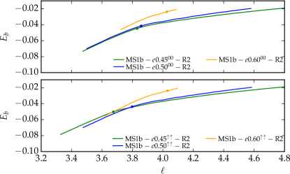
Figure 5: Binding energy vs. specific angular momentum curves $E_{b}(\ell)$ for MS1b EOS for nonspinning (top panel) and aligned spin configurations (bottom panel). The moments of merger are marked by circles.

For a qualitative discussion of the conservative dynamics of the system, we compute the binding energy $E_{b}$ and specific angular momentum $\ell$ from our numerical simulations, see, e.g., Damour et al. (2012); Bernuzzi et al. (2014a); Dietrich and Hinderer (2017).

As examples, we show in Fig. 4 and Fig. 5 the binding energy for the nonspinning (top panel) and spin-aligned (bottom panel) SLy and MS1b configurations respectively. For increasing eccentricity, we find that the curves start with less angular momentum, even though the initial distance is fixed. In the limit of $e\nearrow 1$, one would obtain an initial specific orbital angular momentum of $\ell=0$, because then, at the star center, the symmetry vector of Eq. (1) and thus the fluid velocity have no component perpendicular to the position vector of the star’s center (i.e., no $y$-component).

During the inspiral, the system emits energy and angular momentum in the form of GWs. In general, for an increasing eccentricity, the slope of the individual curves increases. Stated differently, the dimensionless frequency $M\hat{\Omega}=\partial E_{b}/\partial\ell$ at a given specific orbital angular momentum is larger for increasing values of the eccentricity. The systems are less bound for larger eccentricities at fixed $\ell$ during the early part of the inspiral as predicted by PN theory; see Ref. Mora and Will (2004). The behavior of the dimensionless frequency with eccentricity is opposite to that predicted by PN theory. The cause of the difference is not clear, but may be due to the fact that most of the energy and angular momentum are lost near periastron, where the PN approximation is not very accurate. In the most extreme case the stars perform a head on collision for which the angular momentum remains zero regardless of the separation. The stars can be almost unbound even for very small (or even zero) angular momentum. This cannot be achieved for setups with decreasing eccentricity.

It is important to notice that close to the merger and after the merger the ordering of the binding energy curves changes. The merger itself is marked by circles in Fig. 4. This observation can be understood as follows. The moment of merger marks the initial configuration for the evolution of the postmerger. Consequently when the angular momentum and binding energy is larger the remnant is less bound and rotates faster, i.e., $\hat{\Omega}$ is larger.

Similar results are obtained for the MS1b EOS: See Fig. 5.

IV.3 Merger remnant

Table 3: Properties of the merger remnant for the SLy cases. We do not report simulations for MS1b since all these setups form a stable MNS. The columns represent: (i) the name of the configuration (ii) the lifetime, $\tau$, of the HMNS formed during our simulation, given in $M_{\odot}$ and in ms; (iii) the final mass of the BH, $M_{\text{BH}}$, if the HMNS collapsed during our simulation; the dimensionless spin of the final BH, $\chi_{\text{BH}}$ and the mass of the disk surrounding the BH, $M_{\text{disk}}$. We also show the quantities computed from different resolutions for some configurations where they are available. The quantities for configurations that did not undergo collapse to a BH are marked with “$-$”.

Name	$\tau$		$M_{\text{BH}}$	$\chi_{\text{BH}}$	$M_{\text{disk}}$
	$[M_{\odot}]$	$[\rm ms]$	$[M_{\odot}]$		$[M_{\odot}]$
SLy$-e0.40^{00}-{\rm R2}$	$1300$	$6.4$	$2.58$	$0.62$	$0.08$
SLy$-e0.45^{00}-{\rm R1}$	$2100$	$10.3$	$2.53$	$0.55$	$0.09$
SLy$-e0.45^{00}-{\rm R2}$	$6000$	$29.6$	$2.45$	$0.48$	$0.13$
SLy$-e0.45^{00}-{\rm R3}$	$>11150$	$>54.9$	$-$	$-$	$-$
SLy$-e0.45^{00}-{\rm R4}$	$3200$	$15.8$	$2.48$	$0.54$	$0.09$
SLy$-e0.50^{00}-{\rm R1}$	$>6820$	$>33.6$	$-$	$-$	$-$
SLy$-e0.50^{00}-{\rm R2}$	$>9085$	$>44.7$	$-$	$-$	$-$
SLy$-e0.50^{00}-{\rm R3}$	$1700$	$8.4$	$2.55$	$0.59$	$0.07$
SLy$-e0.50^{00}-{\rm R4}$	$2700$	$13.3$	$2.51$	$0.56$	$0.09$
SLy$-e0.60^{00}-{\rm R2}$	$>13100$	$>64.5$	$-$	$-$	$-$
SLy$-e0.40^{\uparrow\uparrow}-{\rm R2}$	$1900$	$9.4$	$2.56$	$0.60$	$0.07$
SLy$-e0.45^{\uparrow\uparrow}-{\rm R1}$	$5400$	$26.6$	$2.42$	$0.46$	$0.16$
SLy$-e0.45^{\uparrow\uparrow}-{\rm R2}$	$2400$	$11.8$	$2.54$	$0.59$	$0.07$
SLy$-e0.45^{\uparrow\uparrow}-{\rm R3}$	$2500$	$12.3$	$2.54$	$0.58$	$0.07$
SLy$-e0.45^{\uparrow\uparrow}-{\rm R4}$	$>10000$	$>49.3$	$-$	$-$	$-$
SLy$-e0.50^{\uparrow\uparrow}-{\rm R2}$	$>9440$	$>46.5$	$-$	$-$	$-$
SLy$-e0.60^{\uparrow\uparrow}-{\rm R2}$	$>8931$	$>44.0$	$-$	$-$	$-$

Due to the choice of the particular total mass of $M\sim 2.7M_{\odot}$, we find in general three different outcomes for our simulations. One possible outcome is the formation of a stable MNS in cases where the total mass of the remnant is below the maximum allowed mass of a spherically symmetric star for the given EOS. Since MS1b supports non-rotating stars with masses up to $\sim 2.76M_{\odot}$, all remnants formed by the merger of the MS1b configurations are indeed MNSs. The SLy EOS instead only supports nonrotating stars with masses up to $\sim 2.06M_{\odot}$. Consequently the remnant is unstable and will collapse to a BH. In fact, the total masses of the remnants formed during the merger of the SLy setups even exceeds the maximum mass of $\sim 2.5M_{\odot}$ of a rigidly rotating SLy star, which is the reason we characterize the remnants as HMNSs  Baumgarte et al. (2000); Hotokezaka et al. (2013a); Baiotti and Rezzolla (2017). Four out of the eight SLy configurations form a BH during the simulation time, at the R2 resolution; one additional configuration only forms a BH during the simulation time at higher resolutions. (The other cases that do not form a BH during the simulation time were not evolved at higher resolutions.) We summarize the properties of the merger remnant for the SLy setups in Table 3. In the following we discuss the lifetime of the merger remnant, the properties of the final BH and the disk masses.

Lifetime of the merger remnant:-

The lifetime and merger properties in our simulations are mostly affected by the total mass of the system and the EOS Hotokezaka et al. (2013a); Dietrich et al. (2015b). It is generally true that systems with a softer EOS collapse earlier than systems with a stiffer EOS. In cases where the EOS is stiff enough, MNSs can form, as in our MS1b simulations. Systems with stiffer EOS are in general less bound at the merger than systems with softer EOS (see Figs. 4 and 5). The relations presented in Read et al. (2013); Bernuzzi et al. (2014b); Takami et al. (2015) also imply that stiffer EOSs lead to merger remnants with larger angular momentum support. In addition to the angular momentum support, the pressure support in the central regions is larger for stiffer EOS, and the merger remnant is even further stabilized. Apart from the dependence on physical quantities, e.g., angular momentum and EOS, the lifetime of the merger remnant is also very sensitive to numerical errors and grid resolutions, as discussed in, e.g.,  Hotokezaka et al. (2013a); Bernuzzi et al. (2014a, 2016). It is thus difficult to quantify the collapse time, and uncertainties can be of the order of several milliseconds (see Table 3). When shocks form, e.g. during the collision of the stars, even high order - high resolution shock capturing methods lose their high convergence properties Bugner et al. (2016); Bernuzzi and Dietrich (2016); Guercilena et al. (2017). We further find that the measurement of the remnant’s lifetime is less robust for eccentric orbits than for quasicircular ones. We think that this is due to the sensitive dependence of the postmerger evolution on the number of close encounters before merger, which itself depends sensitively on the eccentricity, spin, and/or resolution; see Appendix A.

Despite these issues, a robust feature seems to be that configurations with larger initial eccentricity with a fixed initial separation have larger angular momentum at the moment of merger, as shown in Figs. 4 and 5. Knowing that the angular momentum of a head-on collision is zero, this implies that there has to be some eccentricity value for which the angular momentum at merger reaches a maximum.

Due to the larger angular momentum at the moment of merger, we expect a delayed BH formation. While we find that this is in agreement with the results at the R2-resolutions for which the largest set of simulations is available, higher resolutions suggest a more complicated picture. A further study to quantify the remnant lifetime is scheduled for the future. On the other hand, the imprint of spin is less clear. While we find that spin aligned with the orbital angular momentum leads to a delayed merger (orbital hang-up effect Campanelli et al. (2006); Bernuzzi et al. (2014a)), it is also seen that more angular momentum and energy in the form of GWs is emitted before the merger and hence the formed merger remnant has less angular momentum leading to a faster collapse.

Black hole and disk properties:-

Four out of the 14 configurations collapse to a BH after the merger during our simulation time at the R2 resolution, and one more collapses when run at higher resolutions. We expect that if we evolved our configurations with the SLy EOS for longer times then all configurations would have formed BHs. In cases where a BH forms, we report the BH mass $M_{\text{BH}}$, the dimensionless spin $\chi_{\text{BH}}$ of the BH, and the mass of the accretion disk $M_{\text{disk}}$ in Table 3.

We find, independent of the exact setup, that systems with a larger lifetime form less massive black holes with generally smaller dimensionless spins, but more massive disks. However, no clear imprint of the eccentricity can be seen, taking into account the uncertainty of the numerical relativity simulations.

V Ejecta and EM Counterparts

V.1 Ejecta

Table 4: Ejecta properties. The columns refer to: the name of the configuration, the mass of the ejecta from the volume integral $M_{\text{ej}}^{\mathcal{V}}$, the mass of the ejecta from the matter flux through coordinate spheres $M_{\text{ej}}^{\mathcal{S}}$, the kinetic energy of the ejecta $T_{\text{ej}}$, the $D$-weighted integral of $v^{2}=v^{i}v_{i}$ of fluid elements inside the orbital plane $\left\langle\bar{v}\right\rangle_{\rho}$ and perpendicular to it $\left\langle\bar{v}\right\rangle_{z}$. We also show the quantities computed from different resolutions for some configurations.

Name	$M_{\text{ej}}^{\mathcal{V}}$	$M_{\text{ej}}^{\mathcal{S}}$	$T_{\text{ej}}$		$\left\langle\bar{v}\right\rangle_{\rho}$	$\left\langle\bar{v}\right\rangle_{z}$
	$[10^{-2}M_{\odot}]$		$[10^{-5}M_{\odot}]$	[$10^{49}$ erg]	$[c]$	$[c]$
SLy$-e0.40^{00}-$R2	$2.06$	$1.96$	$55.0$	$98.3$	$0.08$	$0.15$
SLy$-e0.45^{00}-$R1	$2.00$	$1.84$	$14.0$	$25.0$	$0.09$	$0.14$
SLy$-e0.45^{00}-$R2	$1.07$	$1.02$	$5.6$	$10.0$	$0.11$	$0.14$
SLy$-e0.45^{00}-$R3	$2.03$	$1.95$	$10.0$	$17.9$	$0.13$	$0.15$
SLy$-e0.45^{00}-$R4	$1.13$	$1.08$	$9.7$	$17.4$	$0.14$	$0.16$
SLy$-e0.50^{00}-$R1	$0.90$	$0.89$	$1.0$	$1.7$	$0.06$	$0.06$
SLy$-e0.50^{00}-$R2	$0.49$	$0.46$	$1.6$	$2.9$	$0.10$	$0.11$
SLy$-e0.50^{00}-$R3	$1.90$	$1.74$	$20.0$	$35.7$	$0.09$	$0.09$
SLy$-e0.50^{00}-$R4	$0.32$	$0.27$	$1.5$	$2.7$	$0.11$	$0.13$
SLy$-e0.60^{00}-$R2	$0.23$	$0.21$	$1.3$	$2.4$	$0.12$	$0.14$
SLy$-e0.40^{\uparrow\uparrow}-$R2	$1.54$	$1.52$	$9.6$	$17.2$	$0.11$	$0.15$
SLy$-e0.45^{\uparrow\uparrow}-$R1	$0.94$	$0.90$	$3.1$	$5.5$	$0.09$	$0.11$
SLy$-e0.45^{\uparrow\uparrow}-$R2	$0.30$	$0.35$	$1.2$	$2.2$	$0.10$	$0.11$
SLy$-e0.45^{\uparrow\uparrow}-$R3	$0.82$	$0.81$	$6.6$	$11.7$	$0.14$	$0.15$
SLy$-e0.45^{\uparrow\uparrow}-$R4	$0.68$	$0.65$	$2.9$	$5.18$	$0.10$	$0.11$
SLy$-e0.50^{\uparrow\uparrow}-$R2	$0.70$	$0.65$	$1.7$	$3.1$	$0.08$	$0.09$
SLy$-e0.60^{\uparrow\uparrow}-$R2	$1.15$	$1.06$	$4.4$	$7.9$	$0.11$	$0.12$
MS1b$-e0.45^{00}-$R2	$1.12$	$1.05$	$2.3$	$4.1$	$0.06$	$0.08$
MS1b$-e0.50^{00}-$R2	$1.55$	$1.49$	$2.8$	$5.0$	$0.06$	$0.08$
MS1b$-e0.60^{00}-$R2	$0.33$	$0.29$	$1.2$	$2.2$	$0.10$	$0.10$
MS1b$-e0.45^{\uparrow\uparrow}-$R2	$1.72$	$1.69$	$6.6$	$11.8$	$0.10$	$0.10$
MS1b$-e0.50^{\uparrow\uparrow}-$R2	$0.90$	$0.85$	$2.0$	$3.5$	$0.08$	$0.09$
MS1b$-e0.60^{\uparrow\uparrow}-$R2	$3.49$	$3.15$	$12.9$	$23.1$	$0.10$	$0.11$

The ejecta masses computed using the two methods briefly described in Sec. II are given in Table 4, where $M_{\text{ej}}^{\mathcal{V}}$ denotes the volume integrated ejecta mass and $M_{\text{ej}}^{\mathcal{S}}$ the ejecta mass computed via Eq. (3), the method of integrating the flux of unbound matter through coordinate spheres. We find good agreement between the two ejecta mass estimates, with differences below 11%.

Considering the effect of resolution, we find that exact quantitative statements about the exact ejecta mass cannot be made and the discussion should just be seen as qualitative. This is often the case for computations of ejecta masses using full 3D NR simulations. Even though simulation methods are continually being improved and simulations are achieving better and better accuracies, the quantification of ejecta material is still challenging and results come with large error bars. It is well known in the NR community that the accuracy of the NR data for quantities such as the unbound mass and kinetic energy have uncertainties which range between $\sim$10% up to even $\sim$100%, see, e.g., Appendix A of Hotokezaka et al. (2013b); Shibata et al. (2017) and Dietrich and Ujevic (2017); Abbott et al. (2017i) for more discussions. Even though there are large uncertainties in the predictions for the ejecta masses, it nevertheless behooves us to understand at least qualitatively the dynamical ejecta mechanisms for eccentric binaries.

We find for the nonspinning SLy (soft EOS) case that the ejecta mass decreases as the eccentricity is increased keeping the initial separation fixed. This is in agreement with East and Pretorius (2012) where equal-mass NSs with comparable compactness of 0.17 and mass of 1.35 have been studied. Reference East and Pretorius (2012) showed that for a decreasing impact parameter $r_{p}$ (equivalent to increasing eccentricity for our cases, see Fig. 2) the amount of unbound matter decreases. For the stiffer EOS (MS1b) setup, we find that they have slightly more unbound matter as compared to the SLy configurations, which is in agreement with, e.g., Dietrich and Ujevic (2017) and is caused by larger tidal tail ejecta.

We find that in the cases where the ejecta mass is $\sim\mathcal{O}(10^{-2})M_{\odot}$, apart from ejecta from tidal tail there is also some ejecta that comes out in the merger-postmerger phase either due to shock heating Rosswog et al. (1999); Oechslin et al. (2006); Bauswein et al. (2013); Wanajo et al. (2014); Sekiguchi et al. (2015); Hotokezaka et al. (2016); Rosswog et al. (2017); Wollaeger et al. (2018); Bovard et al. (2017) when the cores of the two NS collide or from redistribution of the angular momentum within the postmerger remnant; see, e.g., Radice et al. (2018).

In comparison with quasicircular binaries, the MS1b cases have ejecta masses about one order of magnitude larger, cf. Dietrich and Ujevic (2017). Similarly, for the SLy case we find that the ejecta mass is slightly larger for most setups as compared to the analogous quasicircular case, but of the same order [$\mathcal{O}(10^{-2})M_{\odot}$]. However, considering the difference among eccentric setups with fixed initial separation, no strong correlation between the exact eccentricity and the ejected mass is visible for all the configurations except the ones with SLy EOS and no spin.

Interestingly, another source for small amounts of unbound matter is grazing close encounters before the merger cf. the top-left and top-right panels of Fig. 3. As the stars undergo more frequent encounters, the unbound matter increases from $\mathcal{O}(10^{-4})M_{\odot}$ to $\mathcal{O}(10^{-3})M_{\odot}$ until merger. Overall, the unbound material at the merger [$\mathcal{O}(10^{-3})M_{\odot}-\mathcal{O}(10^{-2})M_{\odot}$] is found to be ejected as a mildly relativistic and mildly isotropic outflow with the velocities $\sim 0.06c-0.15c$.

V.2 EM counterparts

As in Refs. Dietrich et al. (2017a, b), we want to present order-of-magnitude estimates for possible electromagnetic counterparts to the merger of these eccentric binary neutron stars.

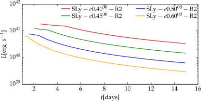
Figure 6: Bolometric luminosity for the SLy setups with zero spin configurations and varying initial eccentricity. The luminosities are computed using the publicly available BNS Kilonova Lightcurve Calculator Dietrich and Kawaguchi . The initial times for the bolometric lightcurves differ due to the different ejecta masses; see discussion in Dietrich and Ujevic (2017).

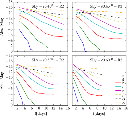
Figure 7: Absolute magnitudes in the ugriz-bands and JHK-bands for the SLy setups with zero spin configurations and varying initial eccentricity. The magnitudes are computed with the BNS Kilonova Lightcurve Calculator available at Dietrich and Kawaguchi ; see Ref. Dietrich and Ujevic (2017) for details.

Kilonovae:-

As a starting point, we follow Grossman et al. (2014) and present a simple estimate for the time $t_{\text{peak}}^{\text{NIR}}$ at which the peak in the near-infrared occurs, as well as an estimate of the corresponding bolometric luminosity at this time $L_{\text{peak}}^{\text{NIR}}$, and the corresponding temperature $T_{\text{peak}}^{\text{NIR}}$. Table 5 summarizes our findings. Overall, we find compatible results for quasicircular and eccentric BNS systems.

In addition to the estimates of the peak time, luminosity, and temperature, we also want to present simple estimates for the time evolution of the bolometric luminosity and the lightcurves in different bands. For this purpose we rely on the analytic approximations of Dietrich and Ujevic (2017) and use the publicly available BNS Kilonova Lightcurve Calculator Dietrich and Kawaguchi . This approach neglects the composition of the ejecta (which is also not evolved in our numerical relativity simulations) and focused on the dynamically ejected matter released during the merger process. Input parameters are taken from Table 4. The latitudinal and the longitudinal opening angles are estimated by evaluation of Eqs. (12) and (13) of Dietrich and Ujevic (2017). Furthermore, we use $\kappa=10\ {\rm cm}^{2}\text{ g}^{-1}$ for the opacity, $\epsilon_{0}=1.58\times 10^{10}\ {\rm erg}\text{ g}^{-1}\text{ s}^{-1}$ for the heating rate coefficient, $\alpha=1.3$ for the heating rate power, and $\epsilon_{th}=0.5$ for the thermalization efficiency as in Dietrich et al. (2017a, b). Figure 6 and Fig. 7 present our results for the time evolution of the bolometric luminosities and the absolute magnitudes for the ugrizJHK bands Fukugita et al. (1996). We find that the configurations we consider will have a luminosity between $10^{39}-10^{42}$ erg s^-1 over a time ranging from a few days to two weeks after the merger (Fig. 6). This will in general be true for all the configurations as the luminosity strongly correlates with the mass of the ejecta, which we have already seen to be $\mathcal{O}(10^{-3})-\mathcal{O}(10^{-2})M_{\odot}$. Therefore, we find in our setups that for an increasing eccentricity the luminosity decreases by more than one order of magnitude for our nonspinning configurations employing the SLy EOS. For other configurations there is no strong correlation between the ejecta masses and the initial eccentricities, as discussed in Sec. V.1.

Radio flares:-

In order to estimate the radio emission caused by the mildly relativistic ejecta, we use the model of Nakar and Piran (2011) which uses as input variables from our simulations the kinetic energy and the velocity of the ejecta. We summarize the quantities for all the configurations studied in this work in Table 5. Most notably we find that radio flares will have largest fluence at $t^{\text{radio}}_{\text{peak}}$ $\sim\mathcal{O}(\rm{years})$ similar to the quasicircular case Dietrich et al. (2017a, b).

Table 5: Properties of electromagnetic counterparts. The columns refer to: the name of the configuration, the time in which the peak in the near infrared occurs $t_{\text{peak}}^{\text{NIR}}$, the corresponding peak luminosity $L_{\text{peak}}^{\text{NIR}}$, the temperature at this time $T_{\text{peak}}^{\text{NIR}}$, the time of peak in the radio band $t^{\text{radio}}_{\text{peak}}$, and the corresponding radio fluence (the flux density per unit frequency) $F^{\nu\text{radio}}_{\text{peak}}$ at 100 Mpc. We present results for all resolutions.

Name	$t_{\text{peak}}^{\text{NIR}}$	$L_{\text{peak}}^{\text{NIR}}$	$T^{\text{NIR}}_{\text{peak}}$	$t^{\text{radio}}_{\text{peak}}$	$F^{\nu\text{radio}}_{\text{peak}}$
	$[\rm{days}]$	$[\rm{10^{40}erg\text{ s}^{-1}}]$	$[\rm{10^{3}K}]$	$[\rm{years}]$	$[\rm{mJy}]$
SLy$-e0.40^{00}-$R2	$5.4$	$4.5$	$1.9$	$15.7$	$0.860$
SLy$-e0.45^{00}-$R1	$5.4$	$4.4$	$1.9$	$10.2$	$0.208$
SLy$-e0.45^{00}-$R2	$3.8$	$3.7$	$2.0$	$6.8$	$0.097$
SLy$-e0.45^{00}-$R3	$4.9$	$5.0$	$1.9$	$6.9$	$0.222$
SLy$-e0.45^{00}-$R4	$3.6$	$4.3$	$2.0$	$6.1$	$0.251$
SLy$-e0.50^{00}-$R1	$5.0$	$2.2$	$2.3$	$12.9$	$0.003$
SLy$-e0.50^{00}-$R2	$2.8$	$2.5$	$2.4$	$6.0$	$0.019$
SLy$-e0.50^{00}-$R3	$6.0$	$3.7$	$1.9$	$18.1$	$0.162$
SLy$-e0.50^{00}-$R4	$2.1$	$2.4$	$2.5$	$4.7$	$0.024$
SLy$-e0.60^{00}-$R2	$1.7$	$2.2$	$2.7$	$3.9$	$0.025$
SLy$-e0.40^{\uparrow\uparrow}-$R2	$4.5$	$4.4$	$1.9$	$7.5$	$0.184$
SLy$-e0.45^{\uparrow\uparrow}-$R1	$4.0$	$3.1$	$2.2$	$8.1$	$0.032$
SLy$-e0.45^{\uparrow\uparrow}-$R2	$2.2$	$2.1$	$2.6$	$5.5$	$0.014$
SLy$-e0.45^{\uparrow\uparrow}-$R3	$3.1$	$3.7$	$2.1$	$5.6$	$0.156$
SLy$-e0.45^{\uparrow\uparrow}-$R4	$3.3$	$2.8$	$2.3$	$7.4$	$0.034$
SLy$-e0.50^{\uparrow\uparrow}-$R2	$3.7$	$2.5$	$2.3$	$8.8$	$0.012$
SLy$-e0.60^{\uparrow\uparrow}-$R2	$4.1$	$3.6$	$2.1$	$7.3$	$0.063$
MS1b$-e0.45^{00}-$R2	$5.2$	$2.6$	$2.2$	$13.2$	$0.011$
MS1b$-e0.50^{00}-$R2	$6.1$	$2.9$	$2.1$	$14.0$	$0.013$
MS1b$-e0.60^{00}-$R2	$2.4$	$2.1$	$2.6$	$6.0$	$0.013$
MS1b$-e0.45^{\uparrow\uparrow}-$R2	$5.4$	$3.8$	$2.0$	$10.5$	$0.068$
MS1b$-e0.50^{\uparrow\uparrow}-$R2	$4.2$	$2.7$	$2.2$	$9.2$	$0.014$
MS1b$-e0.60^{\uparrow\uparrow}-$R2	$7.5$	$5.0$	$1.7$	$12.1$	$0.149$

VI Gravitational Waves

VI.1 Inspiral

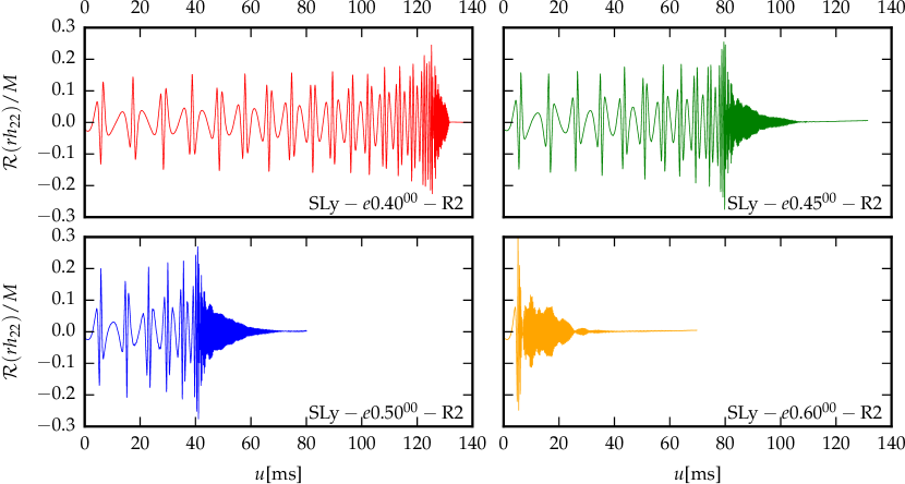
Figure 8: Real part of the (2,2) mode of the gravitational wave strain $rh$ vs. the retarded time $u$. The color code refers to Fig. 1 and corresponds to different eccentricities. See, e.g., Hinder et al. (2018) for eccentric BBH waveforms, for comparison (albeit for smaller eccentricities).

We extract GWs and metric multipoles following Ref. Brügmann et al. (2008). The $\ell=m=2$ multipoles of the GWs extracted at $r=900M_{\odot}$ are shown in Fig. 8 for the configurations employing SLy EOS and no spin. The metric multipoles $rh_{\ell m}$ are reconstructed from the curvature multipoles using the fixed frequency integration of Reisswig and Pollney (2011). We set the low-frequency cutoff to be half the initial GW frequency.

The emission from the orbital motion is very different from the characteristic chirping signal of quasicircular orbits, in which frequency and amplitude monotonically increase. One of the interesting features is the effect of eccentricity. In Fig. 8, one can see that the usual oscillations in the strain at twice the orbital frequency are modulated by an oscillating envelope with a frequency lower than the orbital frequency, corresponding to apsidal precession of the pericenter. A notable feature for BNSs on eccentric orbits is the quasinormal mode oscillations of the NSs as already discussed in Sec. II.3. These oscillations are superposed on the GW signal from the binary’s orbital motion. While the NS oscillations are hardly visible in the metric multipole $rh_{22}$, they are evident in the curvature multipoles. In Fig. 9, we plot the (2,2) mode of $r\Psi_{4}$ and the corresponding instantaneous GW frequency for the SLy$-e0.50^{00}-{\rm R4}$ case, focusing on the inspiral part. The figure also shows consistency of the extracted GW signals at different extraction radii, and in general other quantities extracted at finite radii from the simulated BNS system. In the lower panel of Fig. 9, we find that the influence of finite radius extraction of the GWs is negligible. Therefore, no radius extrapolation to compensate for the finite radius extraction Bernuzzi and Dietrich (2016) is employed. It is reassuring that the GW frequency computed from the phase of the GWs matches twice the orbital frequency computed from the star trajectories during close encounters. Furthermore, comparing with the plot of the instantaneous GW frequency for eccentric BBHs in Ref. Hinder et al. (2018), we find for the BBH case there is no frequency higher than twice the orbital frequency whereas for the BNS case we find a much higher frequency due to the $f$-mode oscillations of the stars.

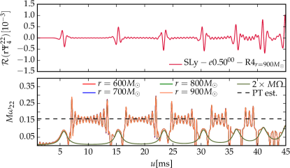
Figure 9: $r\Psi^{22}_{4}$ extracted at $r=900M_{\odot}$ and instantaneous GW frequency $M\omega_{22}$ computed from the phase of $r\Psi^{22}_{4}$ (note that the curves at different extraction radii are coincident) plotted alongside $2\times M\Omega$ as computed from the coordinate tracks of the NSs, both for the inspiral part of the SLy$-e0.50^{00}-{\rm R4}$ case. We find a good agreement for the relation $M\omega_{22}=2\times M\Omega$ and similar results hold for all the other cases. The higher frequency in-between the periastron encounters correspond to the quasinormal mode excitations of the NSs. We also plot the perturbation theory (PT) estimate for the $f$-mode frequency as a black dashed line.

VI.2 f-mode oscillations

Figure 10 and Fig. 11 (left panels) show the (normalized) spectrogram for SLy$-e0.50^{00}-{\rm R2}$ and SLy$-e0.50^{\uparrow\uparrow}-{\rm R2}$, respectively. The right panels show the PSDs for the premerger (black) and postmerger (crimson) phases as different colors for the individual modes. The color bar in the spectrogram goes from red to blue and is given in arbitrary units, since we are only interested in the frequencies and the relative strength.

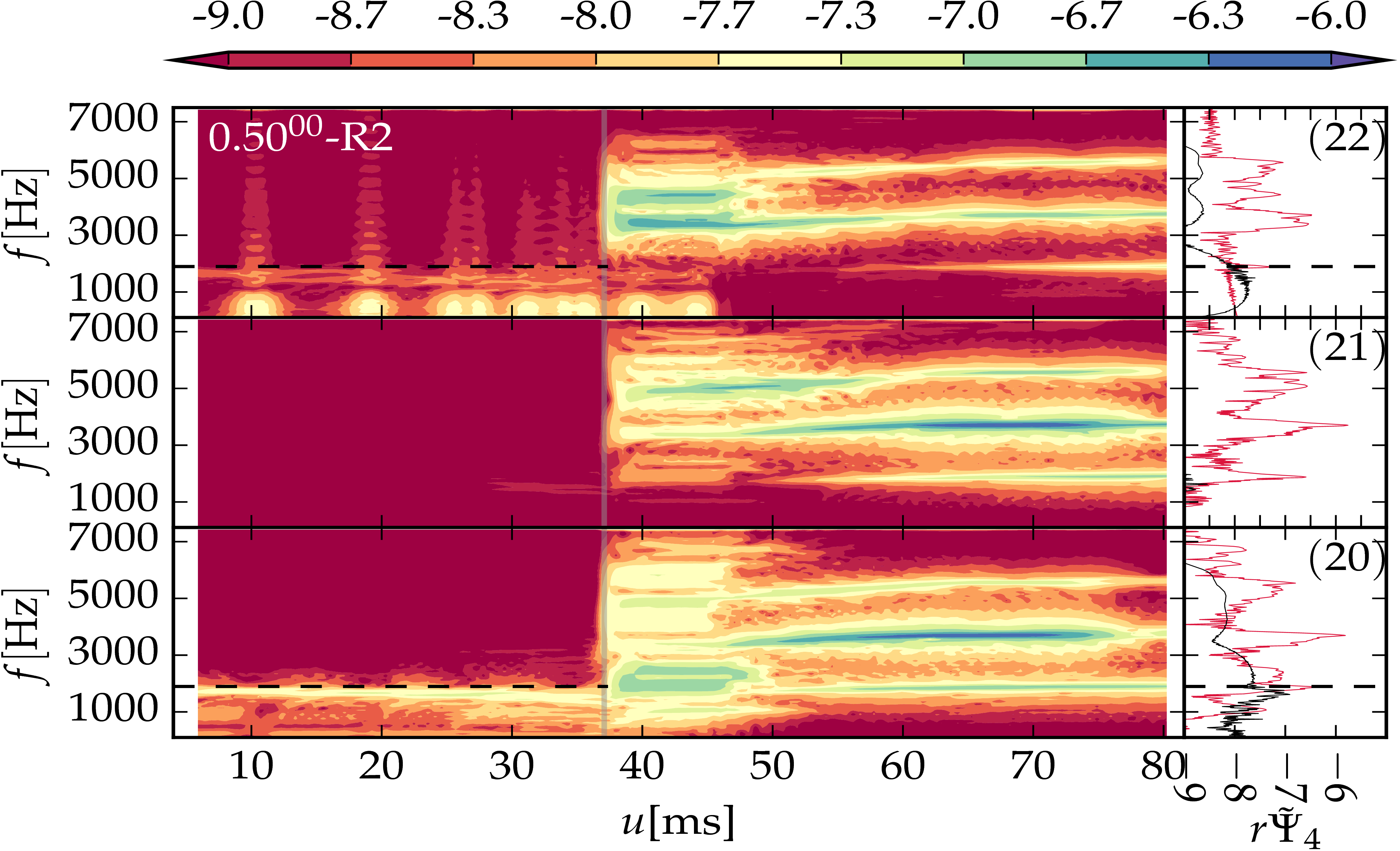
Figure 10: Spectrogram (left) and power spectral density (right) of the curvature scalar $r\Psi_{4}$ for the SLy$-e0.50^{00}-{\rm R2}$ configuration. The labels in the right panel plot refer to the (22), (21), and (20) modes of the curvature scalar. The black dashed line marks the PT estimate of the f-mode frequency and the gray line marks the moment of merger. The PSD is split into a part before the moment of merger (black) and a part after the merger (crimson).

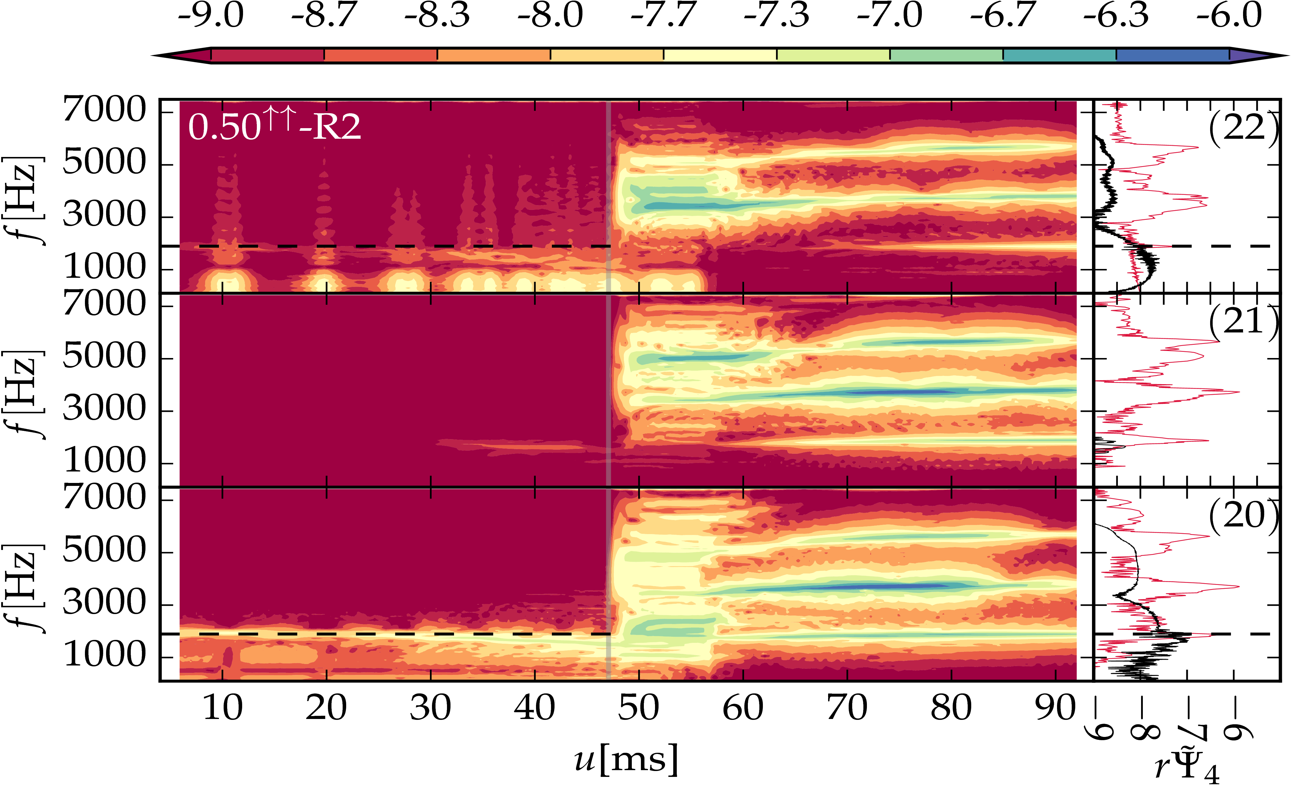
Figure 11: Spectrogram (left) and power spectral density (right) of the curvature scalar $r\Psi_{4}$ for the SLy$-e0.50^{\uparrow\uparrow}-$R2 configuration. The labels in the right panel plot refer to the (22), (21), and (20) modes of the curvature scalar. The black dashed line marks the PT estimate of the f-mode frequency for nonspinning stars and the gray line marks the moment of merger. The PSD is split into a part before the moment of merger (black) and a part after the merger (crimson).

During the inspiral one observes discrete GW bursts present in the $(2,2)$ mode. This is in contrast to the typical chirp signal for the quasicircular orbits, where the frequency and the amplitude increase monotonically over time. We also find a low power, but higher frequency region (1.5 kHz - 2 kHz) distinct from the inspiral burst signals. Such a frequency region is prominent for cases where the NSs’ distance decreases to values as small as 40km-60km (cf. Fig. 2) during the periastron encounters. Thus, we are easily able to extract the NS oscillation frequencies for the configurations for which we set the initial eccentricity, $e$, to be $0.45$ or $0.50$.

The matter mode excitations can be reliably confirmed by studying the spectra of the $(2,0)$ fluid mode excitations. For BNS (and BHNS) in eccentric orbits, the $(2,0)$ fluid mode is expected to be excited as the stars undergo periastron passage (see, e.g., the Newtonian calculations in Yang et al. (2018)). However, the spectrogram in the bottom panel of Fig. 10 for the $(2,0)$ curvature scalar mode, where a relatively high power signal is visible at $\sim 1.8$kHz during the inspiral phase is accounted almost entirely by mode-mixing from (2,$\pm$2) modes, as we will see in the following discussion. We compute the perturbation theory (PT) estimate of the $f$-mode excitation frequency for the SLy EOS with no spin of the NSs using the f-Love relation from Chan et al. (2014), obtaining an f-mode frequency of $1.89$ kHz. As visible in the spectrogram, Fig. 10, there is good agreement between the NS oscillation frequency from the simulation and the PT estimate of the f-mode frequency (horizontal black dashed line). Some of the differences between the PT estimate and the spectrogram are attributable to the gravitational redshift due to the star’s companion, as discussed below, while others are due to the relatively low resolution of the simulation (R2): The f-mode frequency observed in the simulations increases with resolution.

In the spinning case, we find in Fig. 11 that the bright area near $1.8$kHz in the $(2,2)$ and the $(2,0)$ mode in Fig. 10 for the nonspinning case is shifted to slightly higher frequencies. Notice that the dashed line in both figures shows the PT estimate for the nonspinning configuration for easier comparison. Overall, we find similar results for the simulations performed at different resolutions for the same configurations, see Appendix A.

To obtain a PT estimate for the f-mode oscillation frequency of spinning configurations, we follow Doneva et al. Doneva et al. (2013). Since we find an increase in the f-mode frequency with spin, we want to consider the $\ell=2$, $m=-2$ mode. Additionally, it is expected that this mode will be excited most strongly in highly eccentric binaries, as discussed in Yang et al. (2018), using Newtonian calculations. For our case, the NSs with SLy EOS are spinning at $f_{\star}\simeq 191$Hz. Since the Doneva et al. results relate the f-mode frequency of a spinning star to that of a nonspinning star with the same central density, we first note that a nonspinning SLy star with the same central density as the spinning star has a mass of $1.42M_{\odot}$ and thus a f-mode frequency of $f^{\text{Cowling}}_{\text{nonspinning}}=1.93$ kHz (obtained using the f-Love relation from Chan et al. (2014)). We then use Eq. (24) in Doneva et al. Doneva et al. (2013), which gives

$$\frac{\omega^{\text{corot, Cowling}}_{\text{spinning}}}{\omega^{\text{Cowling}}_{\text{nonspinning}}}=1-0.235\frac{\Omega_{\star}}{\Omega_{\text{K}}}-0.543\left(\frac{\Omega_{\star}}{\Omega_{\text{K}}}\right)^{2}.$$ (13)

Here $\omega^{\text{corot, Cowling}}_{\text{spinning}}=\omega^{\text{Cowling}}_{\text{spinning}}-2\Omega_{\star}$ is the mode’s angular frequency in the frame corotating with the star, where $\omega^{\text{Cowling}}_{\text{spinning}}$ is the mode’s angular frequency in the inertial frame of an external observer and $\Omega_{\star}=2\pi f_{\star}$ is the angular velocity of the star. We have $\Omega_{\star}/\Omega_{\text{K}}=0.157$ for these SLy stars, where $\Omega_{\text{K}}$ is the Kepler angular velocity for an SLy star with the same central density as the stars we consider (computed using LORENE Gourgoulhon et al. ). Additionally, we have used superscripts of “Cowling” to denote that the expression in Doneva et al. is derived using the Cowling approximation.

The Cowling approximation generally overestimates the f-mode frequency, as illustrated in, e.g., Fig. 5 in Ref. Zink et al. (2010). However, this figure shows that this overestimate is independent of spin (to a good approximation, particularly for the relatively small spins we are considering). Thus, we can use the Cowling approximation offset of $\Delta f_{\text{Cowling}}\simeq 500$ Hz for a $1.42M_{\odot}$ nonspinning star obtained from Fig. 8 in Ref. Chirenti et al. (2015) to correct for the effect of the approximation (which is, however, only a $\sim 1\%$ effect on the final value). Specifically, if we write $\omega^{\text{corot, Cowling}}_{\text{spinning}}=:k\omega^{\text{Cowling}}_{\text{nonspinning}}$ (so $k=0.95$ here), we have

$$\omega_{\text{spinning}}^{f\text{-mode}}=k\omega_{\text{nonspinning}}^{f\text{-mode}}+2\pi(k-1)\Delta f_{\text{Cowling}}+2\Omega_{\star}.$$ (14)

This procedure gives a f-mode frequency of $2.20$ kHz.

The redshifted PT estimate of the frequency is $\sim 5\%$ larger than the frequency observed in the spectrogram or the instantaneous frequency we compute using the method given below. One would need the spin of the stars to be $\sim 40\%$ smaller than its actual value in order for the instantaneous frequency estimated from the waveform to agree with the redshifted PT frequency. Such a large difference in spin is well outside the maximum expected difference between the true value of the spin and the one estimated from the inputs to the initial data construction, as discussed in Ref. Dietrich et al. (2017b). (Note that the spin we estimate from the initial data inputs agrees well with the one we compute in the early part of the inspiral using the quasilocal computation described in Ref. Dietrich et al. (2017b).) Thus, we are not sure of the source of the discrepancy between the PT estimate and the frequency of the oscillations observed in the simulation. Additionally, there do not appear to be any other $m=\pm 2$ modes that would occur at the observed frequency.

In order to see the effects of the redshift, we can examine the instantaneous f-mode frequency we obtain from the $(2,2)$ mode after removing the orbital contribution (as described in Sec. II.3). This is shown in Fig. 12. (Since $\mu_{2,2;2,2}$ is real, accounting for mode mixing does not change the instantaneous frequency here.) Here we estimate this redshift using the stars’ tracks and the leading PN expression of $\omega_{f\text{-mode}}^{\text{redshifted}}=(1-M^{B}/d)\omega_{f\text{-mode}}$ (see, e.g., Ref. Krisher (1993)), where $d$ is the separation of the two stars, noting that it suffices to consider only star $A$, as the binary is symmetric. The remaining oscillations of the instantaneous frequency are likely due to a combination of the effects mentioned below in the discussion of the $(2,0)$ mode amplitude, as well as the lack of removal of the $(2,2)\leftrightarrow(2,-2)$ mixing (which does not seem straightforward to remove), and possibly also mixing in of intrinsic higher-$\ell$ modes.

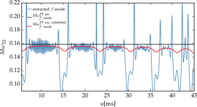
Figure 12: Instantaneous frequency of $\Psi^{4,f\text{-mode}}_{2,2}$ for SLy$-e0.50^{00}-$R4, compared to the prediction of the f-mode frequency of an isolated star, as well as the f-mode frequency including the estimated gravitational redshift due to the star’s companion. These curves should only be compared away from the periastron bursts.

Removing displacement-induced mode mixing in the GW signal from tidally-induced oscillations:-

We now want to apply the displacement-induced mode mixing analysis from Sec. II.3 to obtain the dominant $(2,\pm 2)$ modes of the f-mode oscillations that would be extracted if the stars were at rest at the origin. We will then use the amplitude of these modes to estimate the energy stored in the f-mode oscillations in the next subsubsection.

If we just have a $(2,\pm 2)$ intrinsic excitation of the stars, we will also obtain a purely real contribution to the $(2,0)$ mode from this intrinsic excitation due to the mode mixing. This contribution is purely real because the extracted $(2,\pm 2)$ modes have the usual relation for nonprecessing binaries of $\Psi^{4}_{2,-2}=\left(\Psi^{4}_{2,2}\right)^{*}$ and we have $\mu_{2,-2;2,-2}=\mu_{2,2;2,2}$ and $\mu_{2,-2;2,0}=\mu_{2,2;2,0}^{*}$, so the contribution to the $(2,0)$ mode from mode mixing is

$$\begin{split}\Psi^{4,\text{mixing from }2,\pm 2}_{2,0}&=\Psi^{4,f\text{-mode}}_{2,2}\mu_{2,2;2,0}/\mu_{2,2;2,2}\\ &\quad+\Psi^{4,f\text{-mode}}_{2,-2}\mu_{2,-2;2,0}/\mu_{2,-2;2,-2}\\ &=2\mathcal{R}(\Psi^{4,f\text{-mode}}_{2,2}\mu_{2,2;2,0}/\mu_{2,2;2,2}).\end{split}$$ (15)

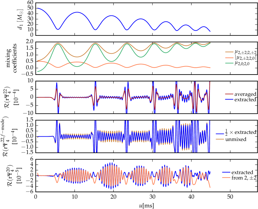
Figure 13: Illustration of the effects of displacement-induced mode mixing on the waveforms extracted from SLy$-e0.50^{00}-$R4: Coordinate distance from star 1 to the origin (top); mode mixing coefficients (second-from-top) ($|\mu_{2,\pm 2;2,\mp 2}|$ is almost indistinguishable from $0$ at this scale, so we do not show it); illustrating the averaging used to separate the $f$-mode and orbital signals (third-from-top); comparing the full mode mixing calculation of the intrinsic f-mode contribution to the real part of the $(2,2)$ mode from a single star to the naive calculation of taking half of the extracted mode (second-from-bottom) (the result for the imaginary part is exactly analogous); comparing the contribution to the real part of the $(2,0)$ mode from mode mixing to that extracted from the evolution of the binary (bottom) (the imaginary part vanishes). In all cases, the approximations used to compute the mode mixing are only valid during the inter-burst f-mode oscillations, and the predictions of the mode mixing calculation for the periastron bursts should not be considered.

In fact, we find that if we compute the mixing coefficients using the tracks to give the positions of the stars, the mixing from the $(2,\pm 2)$ modes appears to account for all of the f-mode signal we extract in the $(2,0)$ mode, as illustrated in Fig. 13. [We use the PT computation of the f-mode frequency used in the previous section. We also checked that we find the expected contributions to the $(3,\pm 2)$ and $(3,0)$ modes due to displacement-induced mode mixing from the $(2,\pm 2)$ modes.] The slight deviations in amplitude are likely due to the approximation of using the coordinate tracks to compute the mixing coefficients and residual contributions from the orbital motion that are not removed by our simple moving average procedure to separate the orbital and f-mode signals. Additionally, while we expect a contribution to the $(2,0)$ mode from the binary’s orbital motion, we find that any such contribution is considerably smaller than the f-mode signal that arises from displacement-induced mode mixing.

We can also use the Schwarzschild tortoise coordinate computed from the tracks instead of the tracks themselves to compute the retarded time, using the system’s ADM mass as the Schwarzschild mass. This is analogous to the procedure used for the extraction of gravitational waves, as described in Sec. V of Dietrich et al. (2017a), though it is less well-motivated here in the stronger-field regime, and we simply consider it to give a comparison for the results computed using the tracks themselves. If we use the tortoise coordinate, then we obtain closer agreement in the amplitude of the mixed contribution to the $(2,0)$ mode and the extracted contribution, but we also obtain intrinsic $(2,\pm 2)$ $f$-mode signals that are considerably larger and look rather unphysical, since their amplitude increases towards apastron. We thus chose to present the results with the plain coordinate track computation.

Energy estimate of the NS oscillations:-

In order to give an order of magnitude estimate of the energy stored in the NS oscillations, we assume that it decays exponentially due to the emission of GWs. We then compute the f-mode GW damping time and use it to infer the energy stored in the NS oscillations by computing the energy radiated in GWs. In particular, we compute the $f$-mode angular frequency using the same f-Love relation from Eq. (3.5) in Chan et al. (2014) used previously, which gives an f-mode frequency of $1.40$ kHz for the nonspinning MS1b stars. The damping time $\tau_{f\text{-mode}}$ (the inverse of the imaginary part of the mode’s angular frequency) is computed using Eq. (20) in Lioutas and Stergioulas (2018), which gives it in terms of the star’s mass and radius. We obtain damping times of $0.186$ s and $0.317$ s, respectively, for the nonspinning SLy and MS1b stars.

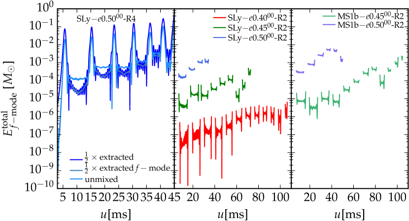
Figure 14: Estimate of the energy stored in f-mode oscillations as a function of the retarded time. (Left panel): Comparison of the results after accounting for displacement-induced mode mixing to those obtained using half the extracted signal, both plain (i.e. the pure extracted signal), and with only the f-mode part for SLy$-e0.50^{00}-$R4. The energy estimate is only valid in the times between the periastron bursts. (Middle and right panels): The energy estimate computed accounting for displacement-induced mode mixing for the nonspinning SLy and MS1b cases that have multiple encounters before merger, considering the R2 resolutions for which we have data for the most eccentricities. In order to clarify these plots, we have excluded the portions of the traces that are close to the periastron bursts.

We compute the energy radiated by using the intrinsic $(2,\pm 2)$ modes of an individual star computed in the previous subsubsection. Since the $f$-mode damping times are much longer than the time between periastra, we assume that the $f$-mode GW signal is exactly sinusoidal, with angular frequency $\omega_{f\text{-mode}}$ and has the same amplitude in both the $(2,2)$ and $(2,-2)$ modes, by symmetry. We then use this to compute the antiderivative of $\Psi_{4}$ (by dividing by $\omega_{f\text{-mode}}$), which gives

$$\dot{E}\simeq\frac{1}{8\pi}\left(\frac{r|\Psi^{4,f\text{-mode}}_{2,2}|}{\omega_{f\text{-mode}}}\right)^{2},$$ (16)

cf. Eq. (52) in Brügmann et al. (2008). Now, the energy stored in the $f$-mode oscillation is $E_{f\text{-mode}}(t)=E_{f\text{-mode}}^{\text{total}}e^{-2t/\tau_{f\text{-mode}}}$. The factor of 2 arises because we are looking at the energy, which goes as the amplitude squared. Thus, we have a radiated energy of $\dot{E}_{\text{GW}}=-\dot{E}_{f\text{-mode}}\simeq(2/\tau_{f\text{-mode}})E_{f\text{-mode}}^{\text{total}}$, where we have evaluated this at $t=0$, by the same argument about the length of the f-mode damping times compared to the time between periastra as above. This finally gives

$$E_{f\text{-mode}}^{\text{total}}\simeq\frac{\tau_{f\text{-mode}}}{16\pi}\left(\frac{r|\Psi^{4,f\text{-mode}}_{2,2}|}{\omega_{f\text{-mode}}}\right)^{2}.$$ (17)

We plot the energy estimate as a function of time for the nonspinning cases in Fig. 14. (We do not include the spinning cases, since we found that the mode mixing removal was not working quite as well for them, likely because the estimate of the f-mode frequency is not sufficiently accurate.) We illustrate how removing the displacement-induced mode mixing is necessary to make an accurate energy estimate, and then compare the energy estimates for the different cases.

We find that the amount of energy stored in the f-mode oscillations increases with initial eccentricity, and is also larger for the MS1b stars than the SLy stars, at a fixed eccentricity. Both of these are to be expected, since the periaston separations decrease with increasing eccentricity, so the stars are experiencing larger tidal perturbations, and the MS1b stars are more tidally deformable than the SLy stars, so they will absorb more energy. We also find that the energy stored in the stars does not always increase monotonically with time, as would be expected, since the tidal perturbations of the stars may be close to out of phase with the already existing oscillations. This is also seen in the analytic calculations in Ref. Yang et al. (2018). (There is a particularly dramatic illustration of such an effect in Fig. 2 of Ref. Radice et al. (2016b), though that paper suggests that it may be an artifact of the $\pi$ symmetry imposed during the evolution.) The remaining time variation of the energy estimate in between periastron encounters is presumably due to the same effects discussed previously for the amplitude of the $(2,0)$ mode from displacement-induced mode mixing and the instantaneous frequency of the f-mode signal. The energy estimates for the first few encounters are robust across resolutions, while the later ones differ more, since the later dynamics also differ between resolutions, as shown for the gravitational waveform in Appendix A.

We find that the f-mode oscillations of the SLy stars store up to $\sim 10^{-3}M_{\odot}$ of energy in the $e=0.5$ case. While $10^{-3}M_{\odot}$ is relatively small compared to some of the other energy scales in the problem (such as the binding energy of the star or the binary’s initial orbital binding energy, which are on the order of $10^{-1}$ and $10^{-2}M_{\odot}$, respectively), it is a tremendous amount of energy, $\sim 10^{51}$ erg, comparable to the energy released in a supernova.

Furthermore, such energies will be sufficient to shatter the NSs’ crust and release the elastic energy stored in these oscillations (cf. Thompson and Duncan (1995) where they report $\sim 10^{46}$ erg to be stored in elastic energy). This will likely lead to flaring activity from milliseconds up to possibly a few seconds before merger (cf. Fig. 14). The signature could be similar to the resonance-induced cracking for quasi-circular inspirals proposed in Tsang et al. (2012), though through different mechanism and time scales. Such a cracking of the NS crust is reported as one possible explanation for sGRB precursors observed by Swift Troja et al. (2010) and might also be visible for BNSs on eccentric orbits.

VI.3 Postmerger

We analyze the GW spectrum of the postmerger waveform by performing a Fourier transform of the simulation data as discussed in Sec. II.

In Table LABEL:tab:postmerger, we report the main peaks identified in the postmerger PSDs from all our configurations including results from different resolution simulations. We analyze the multipolar $r\Psi_{4}^{\ell m}$ modes of the curvature scalar and observe that modes other than (2,2) are also excited during the postmerger phase. These mode frequencies are labeled $f_{1}$, $f_{2}$, $f_{3}$ and are clearly harmonic, i.e., $f_{1}\simeq f_{2}/2\simeq f_{3}/3$; cf. Ref. Dietrich et al. (2015a). These frequencies are extracted in the postmerger phase, i.e., after the peak of the amplitude of the $(2,2)$ mode. For a clear interpretation, we extract the $f_{1}$ frequency from the $(2,1)$ mode and the $f_{3}$ frequency from the $(3,3)$ mode, but they are present in all the modes. The spectra are mainly characterized by a dominant emission frequency $f_{2}$, related to the $(2,2)$ mode.

We also report the GW frequency at merger as $f_{\rm mrg}$. We find that the dimensionless frequency at merger $M\omega_{\rm mrg}$ depends on the EOS. While stiffer EOSs merge with a lower frequency, softer EOSs merge at higher frequencies. Furthermore, we observe a growing $m=1$ mode after the merger, as has been found previously in both quasicircular and eccentric configurations, e.g., Refs. Paschalidis et al. (2015); Lehner et al. (2016); Radice et al. (2016a). We find that the $m=1$ mode is an order-of-magnitude stronger in the SLy cases than in the MS1b cases, but that $m=1$ mode growth in the spinning cases is similar to that in the irrotational cases.

In cases where a HMNS is formed and in particular for configurations undergoing gravitational collapse within dynamical times, the postmerger signal is shorter and the peaks at specific frequencies $f_{1}$, $f_{2}$, $f_{3}$ are more difficult to extract than for configurations that form MNSs. Overall, no direct correlation between initial eccentricity and postmeger frequencies is observed.

Table 6: Post-merger properties. The columns give the name of the configuration, the dimensionless merger frequency $M\omega_{\rm mrg}$, the dimensionful merger frequency $f_{\rm mrg}$ (in kHz), and the dominant postmerger frequencies extracted from the $(2,1)$, $(2,2)$, and $(3,3)$ modes. We mark “$-$” for cases where the frequencies could not be extracted properly, mostly due to the shorter lifetime of the HMNS.

Name	$M\omega_{\text{mrg}}$	$f_{\rm mrg}$	$f_{1}$	$f_{2}$	$f_{3}$
		[kHz]	[kHz]	[kHz]	[kHz]
SLy$-e0.40^{00}-$R2	$0.153$	$1.83$	$-$	$3.51$	$-$
SLy$-e0.45^{00}-$R1	$0.149$	$1.78$	$-$	$3.45$	$-$
SLy$-e0.45^{00}-$R2	$0.165$	$1.97$	$-$	$3.64$	$-$
SLy$-e0.45^{00}-$R3	$0.156$	$1.87$	$1.77$	$3.54$	$5.33$
SLy$-e0.45^{00}-$R4	$0.165$	$1.97$	$-$	$3.66$	$-$
SLy$-e0.50^{00}-$R1	$0.158$	$1.89$	$1.78$	$3.56$	$-$
SLy$-e0.50^{00}-$R2	$0.167$	$1.99$	$1.86$	$3.69$	$5.53$
SLy$-e0.50^{00}-$R3	$0.160$	$1.91$	$-$	$-$	$-$
SLy$-e0.50^{00}-$R4	$0.158$	$1.89$	$-$	$3.47$	$-$
SLy$-e0.60^{00}-$R2	$0.151$	$1.81$	$1.78$	$3.56$	$5.49$
SLy$-e0.40^{\uparrow\uparrow}-$R2	$0.152$	$1.82$	$1.78$	$3.54$	$-$
SLy$-e0.45^{\uparrow\uparrow}-$R1	$0.140$	$1.67$	$1.81$	$3.45$	$-$
SLy$-e0.45^{\uparrow\uparrow}-$R2	$0.169$	$2.01$	$-$	$3.46$	$5.17$
SLy$-e0.45^{\uparrow\uparrow}-$R3	$0.177$	$2.12$	$-$	$3.52$	$-$
SLy$-e0.45^{\uparrow\uparrow}-$R4	$0.178$	$2.12$	$1.80$	$3.62$	$5.43$
SLy$-e0.50^{\uparrow\uparrow}-$R2	$0.157$	$1.87$	$1.87$	$3.72$	$5.62$
SLy$-e0.60^{\uparrow\uparrow}-$R2	$0.139$	$1.65$	$1.72$	$3.47$	$5.17$
MS1b$-e0.45^{00}-$R2	$0.116$	$1.36$	$1.07$	$2.06$	$3.16$
MS1b$-e0.50^{00}-$R2	$0.112$	$1.32$	$1.05$	$2.11$	$3.16$
MS1b$-e0.60^{00}-$R2	$0.112$	$1.32$	$1.05$	$2.11$	$3.16$
MS1b$-e0.45^{\uparrow\uparrow}-$R2	$0.128$	$1.50$	$1.08$	$2.15$	$3.21$
MS1b$-e0.50^{\uparrow\uparrow}-$R2	$0.126$	$1.48$	$1.07$	$2.17$	$3.12$
MS1b$-e0.60^{\uparrow\uparrow}-$R2	$0.106$	$1.25$	$1.10$	$2.17$	$3.24$

VII Summary

In this article, we present and analyze a number of full GR numerical simulations of eccentric BNS mergers with consistent ID employing either irrotational or aligned-spin stars. We systematically vary the initial eccentricity in our simulations to isolate the effect of (large) eccentricity with a fixed initial separation of the NSs. Out of the total of 23 simulations (including different physical configurations as well as different resolutions) presented in this article, 21 of them have been made freely available in Dietrich et al. (2018); CoR ; the remaining $2$ simulations will be made public in the near future. In the following we summarize our findings.

Dynamics:-

We find that depending on the initial eccentricity, the number of orbits significantly varies (starting from a fixed coordinate separation of the stars), ranging from half an orbit for the most eccentric system to as many as $\sim 18$ orbits for the $e=0.40$ configuration employing the SLy EOS and aligned spins. Since some of the simulations are evolved for more than 140 ms to capture the full dynamics of the system, these are among the longest full GR numerical evolutions of BNSs performed to date (in particular SLy$-e0.40^{\uparrow\uparrow}-$R2 with a length of $\approx 172\ {\rm ms}$); see also Haas et al. (2016) and De Pietri et al. (2018) for the longest simulations of quasi-circular BNS inspirals, concentrating on the inspiral and postmerger phases, respectively. For the configurations with aligned-spins, and in particular for systems which undergo multiple non-merging encounters before the merger, we also find that more angular momentum and energy is emitted before the merger, compared to equivalent nonspinning configurations. For the masses and EOSs we consider here, the merger remnant either forms a stable MNS remnant or forms a HMNS which will eventually collapse to a BH. In fact, several evolved systems with SLy EOS form a BH even during the simulation time.

As expected, the properties of the merger remnant are not only dependent on the physical properties such as EOS or initial intrinsic spin, but also depend on the grid resolutions used to evolve the system. Overall, we find that the measurement of the remnant’s lifetime is less robust for the eccentric simulations we consider than for quasicircular orbits. One reason could be the sensitive dependence of the postmerger evolution on the number of close encounters before merger, which itself depends on the eccentricity, spin, and/or resolution. Furthermore, we do not find any clear imprint of eccentricity on the merger remnant properties in general. Thus, quantitative statements must await future work when much higher resolution evolutions are available.

Ejecta and EM counterparts:-

We successfully tested a new routine in BAM for computing unbound matter that minimizes errors introduced in estimating ejecta mass due to the presence of an artificial atmosphere. Good agreement between the new method and the old one with differences in the estimates of the unbound masses below 11% is achieved.

Even though we do not obtain clean convergence for the estimates of the unbound matter with increasing resolution, our results are in good agreement with the few comparable results available in the literature  Stephens et al. (2011); East and Pretorius (2012); East et al. (2016a, b); Radice et al. (2016b). Specifically, $\sim\mathcal{O}(10^{-2})~{}M_{\odot}$ of matter can be ejected at the merger. This is slightly more than in the quasicircular case for the SLy binaries, and about an order of magnitude more for the MS1b binaries. In our simulations tidal tail ejecta are more prominent compared to shock-heated ejecta or ejecta due to the redistribution of angular momentum in the postmerger remnant. Moreover, unbound matter $\sim\mathcal{O}(10^{-3})-\mathcal{O}(10^{-2})~{}M_{\odot}$ is ejected as a mildly relativistic and mildly isotropic outflow with velocities $\sim 6-15$% of the speed of light.

For EM transients we find compatible results for quasicircular and eccentric BNS mergers. In general, the considered configurations will produce kilonovae with luminosities between $10^{39}-10^{42}$ erg s^-1 over a time ranging from a few days to two weeks after the merger. On the other hand, the radio flares will have the largest fluence at $t^{\text{radio}}_{\text{peak}}$ $\sim\mathcal{O}(\text{years})$, similar to equivalent quasicircular cases.

Moreover, in contrast to noneccentric mergers, we find that unbound matter of $\sim\mathcal{O}(10^{-4})-\mathcal{O}(10^{-3})~{}M_{\odot}$ of neutron rich material can be ejected before the merger i.e. during the binary’s successive periastron encounters. This would in principle allow for observations of EM emissions before the merger, although observatories would require early notice.

Gravitational Waves:-

A notable feature for BNSs on eccentric orbits is the superposition of gravitational waves from the quasinormal modes of the NSs (specifically the f-mode) on the GW signal from the binary’s orbital motion. These quasinormal modes are excited by the time-varying tidal perturbations of the stars during their periastron passages.

We find good agreement between the f-mode frequency from our simulations for the irrotational cases and the one obtained from the perturbation theory estimate for an equivalent isolated NS. The $(2,0)$ f-mode signal found in our simulations is accounted for entirely by mode mixing of the intrinsic $(2,\pm 2)$ modes of the stars due to the stars’ displacement from the origin. We also estimate the energy stored in the f-mode oscillations and find that it increases with increasing eccentricity. In general, stiff EOSs, as MS1b, store more energy in the oscillations compared to soft EOSs, e.g. SLy. Additionally, the energy stored in the oscillations of the stars does not always increase monotonically with time. This is to be expected, since for some encounters the tidal perturbations will be out of phase with the already existing oscillations. Overall, these oscillations can store $\sim\mathcal{O}(10^{-8})-\mathcal{O}(10^{-3})~{}M_{\odot}$ of energy depending on eccentricity and the sequence of non-merging encounters.

We find the same qualitative relation between the merger frequency and the stiffness of the EOS that is known for quasicircular binaries, where binaries constructed using the stiffer MS1b EOS merge at lower frequencies than those constructed using the softer SLy EOS. In the postmerger signal modes other than $(2,\pm 2)$ modes are also excited and the same harmonic relation between the dominant frequencies found for quasicircular binaries holds.

With regard to the observability of eccentric BNS mergers, the most prominent features are the burst of gravitational radiation associated with each close encounter, which might be observable with future 3G detectors. On the other hand, observing the f-mode oscillations might require even higher sensitivities or fortuitous circumstances for 3G detectors. If observable, an interesting and notable characteristic would be the change in the f-mode amplitude after each encounter, which may increase or decrease as discussed in Sec. VI.

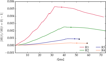
Figure 15: Rest mass conservation of SLy$-e0.50^{00}$ case on refinement level $l=1$. The panel shows the absolute error of the rescaled mass evolution of the baryonic mass. We mark the moment of merger as circles and the moment when a BH forms with a star. The error in the total mass stays below 0.6% for the lowest resolution and below 0.01% for the highest resolution over the entire evolution time. Mass conservation is not violated once a BH forms.

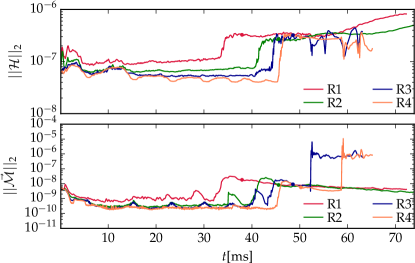
Figure 16: ADM constraints for the SLy$-e0.50^{00}$ case. The upper panel shows the $L^{2}$ volume norm of the Hamiltonian constraint, $||\mathcal{H}||_{2}$. The lower panel shows the Euclidean norm of the $L^{2}$ volume norms of the Cartesian components of the momentum constraint, $||\vec{\mathcal{M}}||_{2}=\sqrt{||\mathcal{M}^{x}||^{2}_{2}+||\mathcal{M}^{y}||^{2}_{2}+||\mathcal{M}^{z}||^{2}_{2}}$. The constraints are evaluated on refinement level 4 and are decreasing for increasing resolution during the inspiral of the neutron stars. Note that here we restrict our convergence analysis to the refinement level 4, cf. Tab. 1. This is needed since for the coarser refinement levels even the higher resolution setups are only barely able to resolve the star whereas for the coarser resolutions not a single point covers the NS leading to a nonconvergent behavior. We have filtered our data with an average filter to give a better visualization and reduce high frequency noise and mark the times of merger by circles.

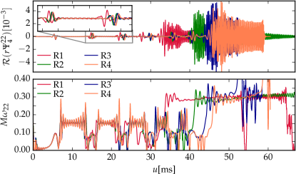
Figure 17: (Top panel): Real part of the curvature multipole $r\Psi^{22}_{4}$ for the SLy$-e0.50^{00}$ configuration for four different resolution, see Table 2. The inset figure shows two periastron encounters and the region in between where the f-mode oscillations are present. (Bottom panel): The instantaneous dimensionless frequency $M\omega_{22}$ computed from $r\Psi^{22}_{4}$. The plots show the robustness of the NS oscillations and the different evolution of the postmerger part. The merger times also vary depending on the resolution due to varying numerical dissipation, which is an inevitable numerical phenomenon for all simulations.

Appendix A Convergence Study

To give some diagnostics for the accuracy of our simulations, we present a convergence study for the conservation of baryonic mass of the system, Fig. 15, the ADM constraints, Fig. 16, and the waveform, Fig. 17, for the SLy$-e0.50^{00}$ configuration. We refer the reader to Refs. Dietrich et al. (2015a); Tichy (2009a) for a detailed discussion about the convergence and accuracy of SGRID and Refs. Bernuzzi et al. (2012); Dietrich et al. (2015b); Bernuzzi and Dietrich (2016) for the accuracy of BAM.

Mass conservation:-

A detailed discussion about the mass conservation in BNS simulations with BAM was presented in Ref. Dietrich et al. (2015b). Here, we want to present the rest mass conservation for at least one of our simulations. Figure 15 shows the mass conservation for the SLy$-e0.50^{00}$ configuration. It is clear that the mass conservation improves with increasing resolution. However, note that the merger itself happens at different times due to different numerical dissipation for different resolutions. Additionally, after the merger no considerable mass loss is present at higher resolutions (except for the cases where a BH forms, which is expected) and the difference to the initial mass stays below 0.6% for the lowest resolution simulation and below 0.01% for the highest resolution simulation.

ADM constraints:-

Since we use a free evolution scheme of the (3+1)-decomposed Einstein equations, we have to ensure that the Hamiltonian and the momentum constraints are fulfilled over the entire simulation. While we explicitly solve the constraints to obtain our initial data, the constraints are not solved during the simulation. Figure 16 shows the L² volume norm of the Hamiltonian constraint (top panel) and the L² volume norm of the square magnitude of the momentum constraint (bottom panel) during the simulation. We see that the constraints are well behaved for the entire duration of the numerical simulation. Oscillations during the inspiral are caused by the movement of inner refinement levels which follow the motion of the neutron stars. After merger those oscillations are absent since the stars stay near the center or only move with a small velocity compared to the inspiral.

Waveform:-

In order to estimate the convergence properties of the GW signal, we use the merger times for the SLy$-e0.50^{00}$ case with multiple resolutions (cf. Fig. 17) presented in this paper.

Considering the merger times computed from the R1, R2, R3, and R4 resolutions, we obtain a convergence of order $\sim 1.5$. While this is an indicator that the simulations are in the convergent regime a more careful investigations, see e.g. Bernuzzi and Dietrich (2016), is needed for a full error assessment. Nevertheless, our results show that the simulations can be used as first test beds once eccentric BNS waveform models become available. But in order to perform detailed waveform modelling and further reduce the uncertainty of our numerical results, even higher resolution simulations are the immediate need. These high resolution simulations will require large amounts of computational resources but are currently underway.

References

- Abbott et al. (2016a) B. P. Abbott et al. (LIGO Scientific Collaboration and Virgo Collaboration), Phys. Rev. Lett. 116, 061102 (2016a), arXiv:1602.03837 [gr-qc] .
- Abbott et al. (2016b) B. P. Abbott et al. (LIGO Scientific Collaboration and Virgo Collaboration), Phys. Rev. Lett. 116, 241103 (2016b), arXiv:1606.04855 [gr-qc] .
- Abbott et al. (2016c) B. P. Abbott et al. (LIGO Scientific Collaboration and Virgo Collaboration), Phys. Rev. X 6, 041015 (2016c), arXiv:1606.04856 [gr-qc] .
- Abbott et al. (2017a) B. P. Abbott et al. (LIGO Scientific Collaboration and Virgo Collaboration), Phys. Rev. Lett. 118, 221101 (2017a), arXiv:1706.01812 [gr-qc] .
- Abbott et al. (2017b) B. P. Abbott et al. (LIGO Scientific Collaboration and Virgo Collaboration), Phys. Rev. Lett. 119, 141101 (2017b), arXiv:1709.09660 [gr-qc] .
- Abbott et al. (2017c) B. P. Abbott et al. (LIGO Scientific Collaboration and Virgo Collaboration), Astrophys. J. Lett. 851, L35 (2017c), arXiv:1711.05578 [astro-ph.HE] .
- Abbott et al. (2017d) B. P. Abbott et al. (LIGO Scientific Collaboration and Virgo Collaboration), Phys. Rev. Lett. 119, 161101 (2017d), arXiv:1710.05832 [gr-qc] .
- Abbott et al. (2017e) B. P. Abbott et al. (LIGO Scientific Collaboration et al.), Astrophys. J. Lett. 848, L12 (2017e), arXiv:1710.05833 [astro-ph.HE] .
- Abbott et al. (2017f) B. P. Abbott et al. (LIGO Scientific Collaboration, Virgo Collaboration, Fermi Gamma-ray Burst Monitor, and INTEGRAL), Astrophys. J. Lett. 848, L13 (2017f), arXiv:1710.05834 [astro-ph.HE] .
- (10) http://www.ligo.caltech.edu/, LIGO - Laser Interferometer Gravitational Wave Observatory.
- (11) http://www.ego-gw.it/, Virgo/EGO, European Gravitational Observatory.
- (12) http://gwcenter.icrr.u-tokyo.ac.jp/en/, KAGRA, Large-scale Cryogenic Gravitational Wave Telescope Project.
- Abbott et al. (2018a) B. P. Abbott et al. (KAGRA Collaboration, LIGO Scientific Collaboration, and Virgo Collaboration), Living Rev. Relativity 21, 3 (2018a), arXiv:1304.0670 [gr-qc] .
- Abbott et al. (2016d) B. P. Abbott et al. (LIGO Scientific Collaboration and Virgo Collaboration), Astrophys. J. Lett. 833, L1 (2016d), arXiv:1602.03842 [astro-ph.HE] .
- Hild et al. (2008) S. Hild, S. Chelkowski, and A. Freise, (2008), arXiv:0810.0604 [gr-qc] .
- Punturo et al. (2010) M. Punturo et al., Classical Quantum Gravity 27, 194002 (2010).
- Ballmer and Mandic (2015) S. Ballmer and V. Mandic, Ann. Rev. Nucl. Part. Sci. 65, 555 (2015).
- Abbott et al. (2017g) B. P. Abbott et al. (LIGO Scientific Collaboration), Classical Quantum Gravity 34, 044001 (2017g), arXiv:1607.08697 [astro-ph.IM] .
- Clark et al. (2014) J. Clark, A. Bauswein, L. Cadonati, H.-T. Janka, C. Pankow, and N. Stergioulas, Phys. Rev. D 90, 062004 (2014), arXiv:1406.5444 [astro-ph.HE] .
- Clark et al. (2016) J. A. Clark, A. Bauswein, N. Stergioulas, and D. Shoemaker, Classical Quantum Gravity 33, 085003 (2016), arXiv:1509.08522 [astro-ph.HE] .
- Radice et al. (2016a) D. Radice, S. Bernuzzi, and C. D. Ott, Phys. Rev. D 94, 064011 (2016a), arXiv:1603.05726 [gr-qc] .
- Radice et al. (2017) D. Radice, S. Bernuzzi, W. Del Pozzo, L. F. Roberts, and C. D. Ott, Astrophys. J. Lett. 842, L10 (2017), arXiv:1612.06429 [astro-ph.HE] .
- Abbott et al. (2017h) B. P. Abbott et al. (LIGO Scientific Collaboration and Virgo Collaboration), Astrophys. J. Lett. 851, L16 (2017h), arXiv:1710.09320 [astro-ph.HE] .
- Hinderer and Babak (2017) T. Hinderer and S. Babak, Phys. Rev. D 96, 104048 (2017), arXiv:1707.08426 [gr-qc] .
- Cao and Han (2017) Z. Cao and W.-B. Han, Phys. Rev. D 96, 044028 (2017), arXiv:1708.00166 [gr-qc] .
- Hinder et al. (2018) I. Hinder, L. E. Kidder, and H. P. Pfeiffer, Phys. Rev. D 98, 044015 (2018), arXiv:1709.02007 [gr-qc] .
- Huerta et al. (2018) E. A. Huerta et al., Phys. Rev. D 97, 024031 (2018), arXiv:1711.06276 [gr-qc] .
- Yang et al. (2018) H. Yang, W. E. East, V. Paschalidis, F. Pretorius, and R. F. P. Mendes, Phys. Rev. D 98, 044007 (2018), arXiv:1806.00158 [gr-qc] .
- Peters (1964) P. C. Peters, Phys. Rev. 136, B1224 (1964).
- Kowalska et al. (2011) I. Kowalska, T. Bulik, K. Belczynski, M. Dominik, and D. Gondek-Rosinska, Astron. Astrophys. 527, A70 (2011), arXiv:1010.0511 [astro-ph.CO] .
- Tsang (2013) D. Tsang, Astrophys. J. 777, 103 (2013), arXiv:1307.3554 [astro-ph.HE] .
- East et al. (2013) W. E. East, S. T. McWilliams, J. Levin, and F. Pretorius, Phys. Rev. D 87, 043004 (2013), arXiv:1212.0837 [gr-qc] .
- (33) M. Abernathy et al., “Einstein gravitational wave Telescope: Conceptual Design Study,” ET-0106C-10.
- Wright (2006) E. L. Wright, Publ. Astron. Soc. Pac. 118, 1711 (2006), arXiv:astro-ph/0609593 [astro-ph] .
- Samsing et al. (2014) J. Samsing, M. MacLeod, and E. Ramirez-Ruiz, Astrophys. J. 784, 71 (2014), arXiv:1308.2964 [astro-ph.HE] .
- Chirenti et al. (2017) C. Chirenti, R. Gold, and M. C. Miller, Astrophys. J. 837, 67 (2017), arXiv:1612.07097 [astro-ph.HE] .
- Peters and Mathews (1963) P. C. Peters and J. Mathews, Phys. Rev. 131, 435 (1963).
- Turner (1977a) M. Turner, Astrophys. J. 216, 610 (1977a).
- Pretorius and Khurana (2007) F. Pretorius and D. Khurana, Classical Quantum Gravity 24, S83 (2007), arXiv:gr-qc/0702084 [gr-qc] .
- Sperhake et al. (2008) U. Sperhake, E. Berti, V. Cardoso, J. A. Gonzalez, B. Brügmann, and M. Ansorg, Phys. Rev. D 78, 064069 (2008), arXiv:0710.3823 [gr-qc] .
- Gold and Brügmann (2010) R. Gold and B. Brügmann, Classical Quantum Gravity 27, 084035 (2010), arXiv:0911.3862 [gr-qc] .
- Gold and Brügmann (2013) R. Gold and B. Brügmann, Phys. Rev. D 88, 064051 (2013), arXiv:1209.4085 [gr-qc] .
- Stephens et al. (2011) B. C. Stephens, W. E. East, and F. Pretorius, Astrophys. J. Lett. 737, L5 (2011), arXiv:1105.3175 [astro-ph.HE] .
- East et al. (2012a) W. E. East, F. Pretorius, and B. C. Stephens, Phys. Rev. D 85, 124009 (2012a), arXiv:1111.3055 [astro-ph.HE] .
- East et al. (2015) W. E. East, V. Paschalidis, and F. Pretorius, Astrophys. J. Lett. 807, L3 (2015), arXiv:1503.07171 [astro-ph.HE] .
- Lee et al. (2010) W. H. Lee, E. Ramirez-Ruiz, and G. van de Ven, Astrophys. J. 720, 953 (2010), arXiv:0909.2884 [astro-ph.HE] .
- Rosswog et al. (2013) S. Rosswog, T. Piran, and E. Nakar, Mon. Not. R. Astron. Soc. 430, 2585 (2013), arXiv:1204.6240 [astro-ph.HE] .
- Gold et al. (2012) R. Gold, S. Bernuzzi, M. Thierfelder, B. Brügmann, and F. Pretorius, Phys. Rev. D 86, 121501(R) (2012), arXiv:1109.5128 [gr-qc] .
- Radice et al. (2016b) D. Radice, F. Galeazzi, J. Lippuner, L. F. Roberts, C. D. Ott, and L. Rezzolla, Mon. Not. R. Astron. Soc. 460, 3255 (2016b), arXiv:1601.02426 [astro-ph.HE] .
- Papenfort et al. (2018) L. J. Papenfort, R. Gold, and L. Rezzolla, (2018), arXiv:1807.03795 [gr-qc] .
- East and Pretorius (2012) W. E. East and F. Pretorius, Astrophys. J. Lett. 760, L4 (2012), arXiv:1208.5279 [astro-ph.HE] .
- East et al. (2016a) W. E. East, V. Paschalidis, F. Pretorius, and S. L. Shapiro, Phys. Rev. D 93, 024011 (2016a), arXiv:1511.01093 [astro-ph.HE] .
- Paschalidis et al. (2015) V. Paschalidis, W. E. East, F. Pretorius, and S. L. Shapiro, Phys. Rev. D 92, 121502 (2015), arXiv:1510.03432 [astro-ph.HE] .
- East et al. (2016b) W. E. East, V. Paschalidis, and F. Pretorius, Classical Quantum Gravity 33, 244004 (2016b), arXiv:1609.00725 [astro-ph.HE] .
- Read et al. (2009) J. S. Read, C. Markakis, M. Shibata, K. Uryū, J. D. Creighton, and J. L. Friedman, Phys. Rev. D 79, 124033 (2009), arXiv:0901.3258 [gr-qc] .
- Turner (1977b) M. Turner, Astrophys. J. 216, 914 (1977b).
- Kokkotas and Schäfer (1995) K. D. Kokkotas and G. Schäfer, Mon. Not. R. Astron. Soc. 275, 301 (1995), arXiv:gr-qc/9502034 [gr-qc] .
- Parisi and Sturani (2018) A. Parisi and R. Sturani, Phys. Rev. D 97, 043015 (2018), arXiv:1705.04751 [gr-qc] .
- Moldenhauer et al. (2014) N. Moldenhauer, C. M. Markakis, N. K. Johnson-McDaniel, W. Tichy, and B. Brügmann, Phys. Rev. D 90, 084043 (2014), arXiv:1408.4136 [gr-qc] .
- Bonazzola et al. (1999) S. Bonazzola, E. Gourgoulhon, and J.-A. Marck, Phys. Rev. Lett. 82, 892 (1999), arXiv:gr-qc/9810072 [gr-qc] .
- Gourgoulhon et al. (2001) E. Gourgoulhon, P. Grandclement, K. Taniguchi, J.-A. Marck, and S. Bonazzola, Phys. Rev. D 63, 064029 (2001), arXiv:gr-qc/0007028 [gr-qc] .
- (62) E. Gourgoulhon, P. Grandclément, J.-A. Marck, J. Novak, and K. Taniguchi, “Lorene code,” http://www.lorene.obspm.fr/.
- East et al. (2012b) W. E. East, F. M. Ramazanoğlu, and F. Pretorius, Phys. Rev. D 86, 104053 (2012b), arXiv:1208.3473 [gr-qc] .
- Tsokaros et al. (2015) A. Tsokaros, K. Uryū, and L. Rezzolla, Phys. Rev. D 91, 104030 (2015), arXiv:1502.05674 [gr-qc] .
- Foucart et al. (2008) F. Foucart, L. E. Kidder, H. P. Pfeiffer, and S. A. Teukolsky, Phys. Rev. D 77, 124051 (2008), arXiv:0804.3787 [gr-qc] .
- Tacik et al. (2015) N. Tacik et al., Phys. Rev. D 92, 124012 (2015), 94, 049903(E) (2016), arXiv:1508.06986 [gr-qc] .
- Tichy (2009a) W. Tichy, Classical Quantum Gravity 26, 175018 (2009a), arXiv:0908.0620 [gr-qc] .
- Tichy (2011) W. Tichy, Phys. Rev. D 84, 024041 (2011), arXiv:1107.1440 [gr-qc] .
- Tichy (2012) W. Tichy, Phys. Rev. D 86, 064024 (2012), arXiv:1209.5336 [gr-qc] .
- Dietrich et al. (2015a) T. Dietrich, N. Moldenhauer, N. K. Johnson-McDaniel, S. Bernuzzi, C. M. Markakis, B. Brügmann, and W. Tichy, Phys. Rev. D 92, 124007 (2015a), arXiv:1507.07100 [gr-qc] .
- Kyutoku et al. (2014) K. Kyutoku, M. Shibata, and K. Taniguchi, Phys. Rev. D 90, 064006 (2014), arXiv:1405.6207 [gr-qc] .
- Dietrich et al. (2017a) T. Dietrich, M. Ujevic, W. Tichy, S. Bernuzzi, and B. Brügmann, Phys. Rev. D 95, 024029 (2017a), arXiv:1607.06636 [gr-qc] .
- Dietrich et al. (2017b) T. Dietrich, S. Bernuzzi, M. Ujevic, and W. Tichy, Phys. Rev. D 95, 044045 (2017b), arXiv:1611.07367 [gr-qc] .
- Abbott et al. (2018b) B. P. Abbott et al. (LIGO Scientific Collaboration and Virgo Collaboration), (2018b), arXiv:1805.11579 [gr-qc] .
- Abbott et al. (2018c) B. P. Abbott et al. (LIGO Scientific Collaboration and Virgo Collaboration), (2018c), arXiv:1805.11581 [gr-qc] .
- Dietrich et al. (2018) T. Dietrich, D. Radice, S. Bernuzzi, F. Zappa, A. Perego, B. Brügmann, S. V. Chaurasia, R. Dudi, W. Tichy, and M. Ujevic, (2018), arXiv:1806.01625 [gr-qc] .
- (77) http://www.computational-relativity.org/, CoRe database of binary neutron star merger waveforms.
- Tichy (2006) W. Tichy, Phys. Rev. D 74, 084005 (2006), arXiv:gr-qc/0609087 [gr-qc] .
- Tichy (2009b) W. Tichy, Phys. Rev. D 80, 104034 (2009b), arXiv:0911.0973 [gr-qc] .
- Wilson and Mathews (1995) J. Wilson and G. Mathews, Phys. Rev. Lett. 75, 4161 (1995).
- Wilson et al. (1996) J. Wilson, G. Mathews, and P. Marronetti, Phys. Rev. D 54, 1317 (1996), arXiv:gr-qc/9601017 [gr-qc] .
- York Jr. (1999) J. W. York Jr., Phys. Rev. Lett. 82, 1350 (1999), arXiv:gr-qc/9810051 [gr-qc] .
- Brügmann et al. (2008) B. Brügmann, J. A. Gonzalez, M. Hannam, S. Husa, U. Sperhake, and W. Tichy, Phys. Rev. D 77, 024027 (2008), arXiv:gr-qc/0610128 [gr-qc] .
- Thierfelder et al. (2011) M. Thierfelder, S. Bernuzzi, and B. Brügmann, Phys. Rev. D 84, 044012 (2011), arXiv:1104.4751 [gr-qc] .
- Dietrich et al. (2015b) T. Dietrich, S. Bernuzzi, M. Ujevic, and B. Brügmann, Phys. Rev. D 91, 124041 (2015b), arXiv:1504.01266 [gr-qc] .
- Bernuzzi and Dietrich (2016) S. Bernuzzi and T. Dietrich, Phys. Rev. D 94, 064062 (2016), arXiv:1604.07999 [gr-qc] .
- Nakamura et al. (1987) T. Nakamura, K. Oohara, and Y. Kojima, Prog. Theor. Phys. Suppl. 90, 1 (1987).
- Shibata and Nakamura (1995) M. Shibata and T. Nakamura, Phys. Rev. D 52, 5428 (1995).
- Baumgarte and Shapiro (1998) T. W. Baumgarte and S. L. Shapiro, Phys. Rev. D 59, 024007 (1998), arXiv:gr-qc/9810065 .
- Bona et al. (1996) C. Bona, J. Massó, J. Stela, and E. Seidel, in The Seventh Marcel Grossmann Meeting: On Recent Developments in Theoretical and Experimental General Relativity, Gravitation, and Relativistic Field Theories, edited by R. T. Jantzen, G. M. Keiser, and R. Ruffini (World Scientific, Singapore, 1996).
- Alcubierre et al. (2003) M. Alcubierre, B. Brügmann, P. Diener, M. Koppitz, D. Pollney, E. Seidel, and R. Takahashi, Phys. Rev. D 67, 084023 (2003), arXiv:gr-qc/0206072 [gr-qc] .
- van Meter et al. (2006) J. R. van Meter, J. G. Baker, M. Koppitz, and D.-I. Choi, Phys. Rev. D 73, 124011 (2006), arXiv:gr-qc/0605030 .
- Bauswein et al. (2010) A. Bauswein, H.-T. Janka, and R. Oechslin, Phys. Rev. D 82, 084043 (2010), arXiv:1006.3315 [astro-ph.SR] .
- Borges et al. (2008) R. Borges, M. Carmona, B. Costa, and W. S. Don, J. Comput. Phys. 227, 3191 (2008).
- Kastaun and Galeazzi (2015) W. Kastaun and F. Galeazzi, Phys. Rev. D 91, 064027 (2015), arXiv:1411.7975 [gr-qc] .
- Boyle (2016) M. Boyle, Phys. Rev. D 93, 084031 (2016), arXiv:1509.00862 [gr-qc] .
- Gualtieri et al. (2008) L. Gualtieri, E. Berti, V. Cardoso, and U. Sperhake, Phys. Rev. D 78, 044024 (2008), arXiv:0805.1017 [gr-qc] .
- Mora and Will (2004) T. Mora and C. M. Will, Phys. Rev. D 69, 104021 (2004), 71, 129901(E) (2005), arXiv:gr-qc/0312082 [gr-qc] .
- Damour and Nagar (2010) T. Damour and A. Nagar, Phys. Rev. D 81, 084016 (2010), arXiv:0911.5041 [gr-qc] .
- Damour et al. (2012) T. Damour, A. Nagar, D. Pollney, and C. Reisswig, Phys. Rev. Lett. 108, 131101 (2012), arXiv:1110.2938 [gr-qc] .
- Bernuzzi et al. (2014a) S. Bernuzzi, T. Dietrich, W. Tichy, and B. Brügmann, Phys. Rev. D 89, 104021 (2014a), arXiv:1311.4443 [gr-qc] .
- Dietrich and Hinderer (2017) T. Dietrich and T. Hinderer, Phys. Rev. D 95, 124006 (2017), arXiv:1702.02053 [gr-qc] .
- Baumgarte et al. (2000) T. W. Baumgarte, S. L. Shapiro, and M. Shibata, Astrophys. J. Lett. 528, L29 (2000), arXiv:astro-ph/9910565 .
- Hotokezaka et al. (2013a) K. Hotokezaka, K. Kiuchi, K. Kyutoku, T. Muranushi, Y.-i. Sekiguchi, M. Shibata, and K. Tanaguchi, Phys. Rev. D 88, 044026 (2013a), arXiv:1307.5888 [astro-ph.HE] .
- Baiotti and Rezzolla (2017) L. Baiotti and L. Rezzolla, Rept. Prog. Phys. 80, 096901 (2017), arXiv:1607.03540 [gr-qc] .
- Read et al. (2013) J. S. Read, L. Baiotti, J. D. E. Creighton, J. L. Friedman, B. Giacomazzo, K. Kyutoku, C. Markakis, L. Rezzolla, M. Shibata, and K. Tanaguchi, Phys. Rev. D 88, 044042 (2013), arXiv:1306.4065 [gr-qc] .
- Bernuzzi et al. (2014b) S. Bernuzzi, A. Nagar, S. Balmelli, T. Dietrich, and M. Ujevic, Phys. Rev. Lett. 112, 201101 (2014b), arXiv:1402.6244 [gr-qc] .
- Takami et al. (2015) K. Takami, L. Rezzolla, and L. Baiotti, Phys. Rev. D 91, 064001 (2015), arXiv:1412.3240 [gr-qc] .
- Bernuzzi et al. (2016) S. Bernuzzi, D. Radice, C. D. Ott, L. F. Roberts, P. Moesta, and F. Galeazzi, Phys. Rev. D 94, 024023 (2016), arXiv:1512.06397 [gr-qc] .
- Bugner et al. (2016) M. Bugner, T. Dietrich, S. Bernuzzi, A. Weyhausen, and B. Brügmann, Phys. Rev. D 94, 084004 (2016), arXiv:1508.07147 [gr-qc] .
- Guercilena et al. (2017) F. Guercilena, D. Radice, and L. Rezzolla, Comput. Astrophys. Cosmol. 4, 3 (2017), arXiv:1612.06251 [gr-qc] .
- Campanelli et al. (2006) M. Campanelli, C. Lousto, and Y. Zlochower, Phys. Rev. D 74, 041501 (2006), arXiv:gr-qc/0604012 [gr-qc] .
- Hotokezaka et al. (2013b) K. Hotokezaka, K. Kiuchi, K. Kyutoku, H. Okawa, Y.-i. Sekiguchi, M. Shibata, and K. Taniguchi, Phys. Rev. D 87, 024001 (2013b), arXiv:1212.0905 [astro-ph.HE] .
- Shibata et al. (2017) M. Shibata, S. Fujibayashi, K. Hotokezaka, K. Kiuchi, K. Kyutoku, Y. Sekiguchi, and M. Tanaka, Phys. Rev. D 96, 123012 (2017), arXiv:1710.07579 [astro-ph.HE] .
- Dietrich and Ujevic (2017) T. Dietrich and M. Ujevic, Classical Quantum Gravity 34, 105014 (2017), arXiv:1612.03665 [gr-qc] .
- Abbott et al. (2017i) B. P. Abbott et al. (LIGO Scientific Collaboration and Virgo Collaboration), Astrophys. J. Lett. 850, L39 (2017i), arXiv:1710.05836 [astro-ph.HE] .
- Rosswog et al. (1999) S. Rosswog, M. Liebendoerfer, F.-K. Thielemann, M. B. Davies, W. Benz, and T. Piran, Astron. Astrophys. 341, 499 (1999), arXiv:astro-ph/9811367 [astro-ph] .
- Oechslin et al. (2006) R. Oechslin, H.-T. Janka, and A. Marek, Astron. Astrophys. 467, 395 (2006), arXiv:astro-ph/0611047 [astro-ph] .
- Bauswein et al. (2013) A. Bauswein, S. Goriely, and H.-T. Janka, Astrophys. J. 773, 78 (2013), arXiv:1302.6530 [astro-ph.SR] .
- Wanajo et al. (2014) S. Wanajo, Y. Sekiguchi, N. Nishimura, K. Kiuchi, K. Kyutoku, and M. Shibata, Astrophys. J. Lett. 789, L39 (2014), arXiv:1402.7317 [astro-ph.SR] .
- Sekiguchi et al. (2015) Y. Sekiguchi, K. Kiuchi, K. Kyutoku, and M. Shibata, Phys. Rev. D 91, 064059 (2015), arXiv:1502.06660 [astro-ph.HE] .
- Hotokezaka et al. (2016) K. Hotokezaka, S. Wanajo, M. Tanaka, A. Bamba, Y. Terada, and T. Piran, Mon. Not. R. Astron. Soc. 459, 35 (2016), arXiv:1511.05580 [astro-ph.HE] .
- Rosswog et al. (2017) S. Rosswog, U. Feindt, O. Korobkin, M. R. Wu, J. Sollerman, A. Goobar, and G. Martinez-Pinedo, Classical Quantum Gravity 34, 104001 (2017), arXiv:1611.09822 [astro-ph.HE] .
- Wollaeger et al. (2018) R. T. Wollaeger, O. Korobkin, C. J. Fontes, S. K. Rosswog, W. P. Even, C. L. Fryer, J. Sollerman, A. L. Hungerford, D. R. van Rossum, and A. B. Wollaber, Mon. Not. R. Astron. Soc. 478, 3298 (2018), arXiv:1705.07084 [astro-ph.HE] .
- Bovard et al. (2017) L. Bovard, D. Martin, F. Guercilena, A. Arcones, L. Rezzolla, and O. Korobkin, Phys. Rev. D 96, 124005 (2017), arXiv:1709.09630 [gr-qc] .
- Radice et al. (2018) D. Radice, A. Perego, S. Bernuzzi, and B. Zhang, (2018), arXiv:1803.10865 [astro-ph.HE] .
- (127) T. Dietrich and K. Kawaguchi, “BNS Kilonova Lightcurve Calculator,” http://computational-relativity.org/tdietrich/kn/main.html.
- Grossman et al. (2014) D. Grossman, O. Korobkin, S. Rosswog, and T. Piran, Mon. Not. R. Astron. Soc. 439, 757 (2014), arXiv:1307.2943 [astro-ph.HE] .
- Fukugita et al. (1996) M. Fukugita, T. Ichikawa, J. E. Gunn, M. Doi, K. Shimasaku, and D. P. Schneider, Astron. J. 111, 1748 (1996).
- Nakar and Piran (2011) E. Nakar and T. Piran, Nature (London) 478, 82 (2011), arXiv:1102.1020 [astro-ph.HE] .
- Reisswig and Pollney (2011) C. Reisswig and D. Pollney, Classical Quantum Gravity 28, 195015 (2011), arXiv:1006.1632 [gr-qc] .
- Chan et al. (2014) T. K. Chan, Y.-H. Sham, P. T. Leung, and L.-M. Lin, Phys. Rev. D 90, 124023 (2014), arXiv:1408.3789 [gr-qc] .
- Bernuzzi et al. (2015) S. Bernuzzi, A. Nagar, T. Dietrich, and T. Damour, Phys. Rev. Lett. 114, 161103 (2015), arXiv:1412.4553 [gr-qc] .
- (134) S. Bernuzzi and A. Nagar, “IHES EOB code,” https://eob.ihes.fr/.
- Doneva et al. (2013) D. D. Doneva, E. Gaertig, K. D. Kokkotas, and C. Krüger, Phys. Rev. D 88, 044052 (2013), arXiv:1305.7197 [astro-ph.SR] .
- Zink et al. (2010) B. Zink, O. Korobkin, E. Schnetter, and N. Stergioulas, Phys. Rev. D 81, 084055 (2010), arXiv:1003.0779 [astro-ph.SR] .
- Chirenti et al. (2015) C. Chirenti, G. H. de Souza, and W. Kastaun, Phys. Rev. D 91, 044034 (2015), arXiv:1501.02970 [gr-qc] .
- Steinhoff et al. (2016) J. Steinhoff, T. Hinderer, A. Buonanno, and A. Taracchini, Phys. Rev. D 94, 104028 (2016), arXiv:1608.01907 [gr-qc] .
- Krisher (1993) T. P. Krisher, Phys. Rev. D 48, 4639 (1993).
- Lioutas and Stergioulas (2018) G. Lioutas and N. Stergioulas, Gen. Relativ. Gravit. 50, 12 (2018), arXiv:1709.10067 [gr-qc] .
- Thompson and Duncan (1995) C. Thompson and R. C. Duncan, Mon. Not. R. Astron. Soc. 275, 255 (1995).
- Tsang et al. (2012) D. Tsang, J. S. Read, T. Hinderer, A. L. Piro, and R. Bondarescu, Phys. Rev. Lett. 108, 011102 (2012), arXiv:1110.0467 [astro-ph.HE] .
- Troja et al. (2010) E. Troja, S. Rosswog, and N. Gehrels, Astrophys. J. 723, 1711 (2010), arXiv:1009.1385 [astro-ph.HE] .
- Lehner et al. (2016) L. Lehner, S. L. Liebling, C. Palenzuela, and P. M. Motl, Phys. Rev. D 94, 043003 (2016), arXiv:1605.02369 [gr-qc] .
- Haas et al. (2016) R. Haas et al., Phys. Rev. D 93, 124062 (2016), arXiv:1604.00782 [gr-qc] .
- De Pietri et al. (2018) R. De Pietri, A. Feo, J. A. Font, F. Löffler, F. Maione, M. Pasquali, and N. Stergioulas, Phys. Rev. Lett. 120, 221101 (2018), arXiv:1802.03288 [gr-qc] .
- Bernuzzi et al. (2012) S. Bernuzzi, M. Thierfelder, and B. Brügmann, Phys. Rev. D 85, 104030 (2012), arXiv:1109.3611 [gr-qc] .