Topologically protected heat pumping from braiding Majorana zero modes

Abstract

Majorana zero modes are non-Abelian quasiparticles that emerge on the edges of topological phases of superconductors. Evidence of their presence have been reported in transport measurements on engineered superconducting-based nanostructures. In this manuscript we identify signatures of a topologically protected dynamical manipulation of Majorana zero modes via continuous transport measurement during the manipulation. Specifically, we show that, in a two-terminal geometry, the heat pumped across the terminals at low temperature and voltage bias is characterized by a universal value. We show that this feature is inherent to the presence of Majorana zero modes and discuss its robustness against temperature, voltage bias and the detailed coupling to the contacts.

Introduction

Majorana zero modes are non-Abelian quasiparticles bound to the surface and to defects in topological supercoductors.Wilczek (1982); Read and Green (2000); Stern (2010) Driven by the promise of exploiting their non-Abelian statistics for fault-tolerant information processing Nayak et al. (2008), proposals for engineering such a topological phase in superconductor-based nanostructures have shifted the focus on Majorana zero modes form a purely theoretical feature Moore and Read (1991); Read and Green (2000); Kitaev (2001) to an experimentally observable entity Fu and Kane (2008); Lutchyn et al. (2010); Oreg et al. (2010). While the first wave of experiments Mourik et al. (2012); Das et al. (2012); Churchill et al. (2013); Nadj-Perge et al. (2014); Albrecht et al. (2016); Deng et al. (2016) were designed solely to detect these exotic excitations, the next generation of experiments Aasen et al. (2016); Plugge et al. (2016a, b) and theoretical proposals Fu (2010); Michaeli et al. (2016); Vijay and Fu (2016); Zocher and Rosenow (2013); Rubbert and Akhmerov (2016); Romito and Gefen (2017) aim at probing directly their non-local topological properties, with the ultimate goal of optimising and controlling their manipulation.

A key feature of topological phases based on superconducting nanostructures is the multitude of available detection schemes. To date, transport properties, such as conductance and tunneling density of states Flensberg (2010), have provided the predominant evidence of Majorana zero modes Mourik et al. (2012); Das et al. (2012); Churchill et al. (2013); Nadj-Perge et al. (2014); Albrecht et al. (2016); Deng et al. (2016), and charge sensing schemes have been proposed to effectively implement braiding protocols Bonderson et al. (2008); Bonderson (2013); Karzig et al. (2017). Indeed, having an open apparatus, where the topological material is coupled to non interacting leads, allows to define new topological invariants based on scattering statesFulga et al. (2011); Meidan et al. (2014, 2016).

In this manuscript we look at an intermediate benchmark towards the implementation and detection of topologically protected operations by examining the transport signatures of a braiding protocol. For this purpose we consider the minimal setup for the exchange of Majorana modes, in a Y-junction layout, see Fig. 1. In a sequence of operations shown in Fig. 2, the Y-junction setup is then driven to perform Majorana braiding. We show that a combination of the density of heat and charge pumped during the braiding cycle is a universal quantity, independent of the details of the driving and of the couplings to the external leads. We further discus how this measurable feature is affected by temperature and by the contact geometry. This universal value stems directly from the geometric properties of the braiding cycle in parameter space, and can be used as a signature of such a topologically protected operation. It also provides a new potential tool for engineering heat pumping device.

Model —

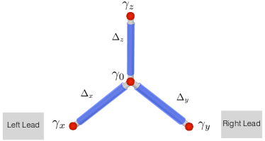
Figure 1: Schematics of a junction of three 1d p-wave superconductors. The Majorana zero-modes at two ends of the junction are connected to external leads. The effective couplings between pairs of Majorana can be tuned independently.

The system we consider is schematically depicted in Fig. 1. It consists of three topological superconducting (TSC) wires arranged in a Y-junction configuration. The wires can be realized in proximity coupled semi conducting wires with a strong spin orbit coupling, subjected to a magnetic field and proximity coupled to a superconductor Oreg et al. (2010); Lutchyn et al. (2010). Throughout the manuscript we will assume that the superconductors are large enough such that charging effects can be neglected. Each topological superconducting wire hosts two Majorana zero modes at its end. At energies well below the induced superconducting gap, $\Delta$, the Hilbert space is spanned by three Majorana bound states $\gamma_{i}$ where $i={x,y,z}$ which appear at the three ends of the Y-junction, and a single Majorana bound state at the center $\gamma_{0}$, as shown in the figure. (The junction may host additional sub gap states. We restrict to energies which are well below any accidental subgap excitations). The four Majorana zero modes can be gapped in pairs, and the effective low energy Hamiltonian of the Y junction is

$$H_{Y} = i\gamma_{0}\vec{\Delta}\cdot\vec{\gamma}$$ (1)

where $\vec{\Delta}=\Delta(\sin\theta\cos\phi,\sin\theta\sin\phi,\cos\theta)$ and $\vec{\gamma}=(\gamma_{x},\gamma_{y},\gamma_{z})$.

In order to study the transport properties of the system we couple the Y-junction to two single channel leads, denoted by $L,R$. The full Hamiltonian is then given by $H=H_{Y}+H_{T}+\sum_{\alpha=L,R}H_{\alpha}$, where

$$H_{T} = t_{L}\left(c_{Lk}-c_{Lk}^{\dagger}\right)\gamma_{x}+t_{R}\left(c_{Rk}-c_{Rk}^{\dagger}\right)\gamma_{y}$$ (2)

$$H_{\alpha} = \sum_{k}\xi_{k}c_{\alpha k}^{\dagger}c_{\alpha k},$$

with $\xi_{\alpha k}$ the lead energy dispersion and with the tunneling charcterised by the rates $\Gamma_{\alpha}=\pi\nu_{\alpha}|t_{\alpha}|^{2}$, $\nu_{\alpha}$ the energy density of sates.

The Y-junction is the simplest proposed setup that allows to perform Majorana braiding. This can be achieved by adjusting the pairwise coupling $\Delta_{i}$ between in an adiabatic sequence using gates or magnetic fluxes van Heck et al. (2012); Karzig et al. (2016). The pairwise coupling sequence and the corresponding cycle in the parameter space are depicted in Fig. 2.

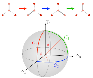
Figure 2: Schematic representation of the driving cycle. Grey lines represent the pairwise coupling between Majoranas ($\Delta_{j}\neq 0$ for full lines and $\Delta_{j}=0$ for dotted lines). The corresponding stages of the evolution are represented as a path in the parameter space spanned by $\vec{\Delta}$.

The induced operation on the state of the system can be better understood by applying an orthogonal rotation on $H_{Y}$ to obtain $H_{Y}^{d}=i\Delta\gamma_{0}\gamma_{r}$, where $\gamma_{r}=\vec{\gamma}\cdot\hat{e}_{r}$, and the two zero modes $\gamma_{\theta}=\vec{\gamma}\cdot\hat{e}_{\theta}$ and $\gamma_{\phi}=\vec{\gamma}\cdot\hat{e}_{\phi}$, with $\hat{e}_{r}$, $\hat{e}_{\theta}$ and $\hat{e}_{\phi}$ the basis vectors in spherical coordinates, and $\hat{e}_{\theta}$ and $\hat{e}_{\phi}$ span a two fold degenerate subspace. The evolution induced by adjusting the pairwise coupling shown Fig. 2 corresponds to adiabatically changing the projection of the Majorana bound states physically coupled to the leads $\gamma_{x,y,z}$ on to the degenerate subspace spanned by $\gamma_{\theta},\gamma_{\phi}$. Importantly the operation is exponentially protected regardless of the fluctuations in controlling the system parameters Karzig et al. (2016).

Adiabatic change of scattering matrix —

The adiabatic manipulation of the system parameters depicted in Fig. 2 can be regarded as pumping cycle when the system is coupled to external leads, see Fig. 1. In order to study the transport properties of the braiding cycle, we compute the scattering matrix defined as $\Psi_{\rm out}(\epsilon)=S(\epsilon)\Psi_{\rm in}(\epsilon)$ where the scattering states $\Psi_{\rm in}=(\Phi_{e,L},\Phi_{h,L},\Phi_{e,R},\Phi_{h,R})$ are in the basis of electrons $(e)$ and holes $(h)$ in the left $(L)$ and right $(R)$ leads. The scattering matrix can be expressed as Mahaux1969 :

$$S(\epsilon)=\openone+2\pi iW^{\dagger}\left(H_{0}-\epsilon-i\pi WW^{\dagger}\right)^{-1}W$$ (3)

Where $W$ is the matrix that encodes the coupling to the leads. Eq. (3) is more transparent in the rotated basis: $\tilde{\Psi}=(\Phi_{L}^{+},\Phi_{R}^{+},\Phi_{L}^{-},\Phi_{R}^{-})$ where $\Phi_{\alpha}^{\pm}=\frac{1}{\sqrt{2}}\left[\Phi_{e,\alpha}\pm\Phi_{h,\alpha}\right]$. From Eq (2) it follows that in this basis the scattering matrix takes a block diagonal form with only two channels coupled to the Y-junction. We therefore restrict to the two dimensional basis of coupled channels, namely $\psi=(\Phi_{L}^{-},\Phi_{R}^{-})$. Here the coupling matrix takes the simplified form $W=\sqrt{2}t_{L}|x\rangle\langle L^{-}|+\sqrt{2}t_{R}|y\rangle\langle R^{-}|$, and the scattering matrix can be written as $S(\epsilon)=\mathbf{1}_{2}\oplus\tilde{S}(\epsilon)$, where the $\tilde{S}(\epsilon)\in U(2)$ is the non-trivial block of the scattering matrix.

At energies well below the induced superconducting gap, $\epsilon\ll\Delta$, only the two fold degenerate ground-space of the Hamiltonian takes part in the transport, and we need to account for the lead-system coupling terms projected on the ground state only. Defining a projection operator $P_{\rm g}=|\theta\rangle\langle\theta|+|\phi\rangle\langle\phi|$, we can rewrite the expression for the scattering matrix in Eq. (3) by replacing $W$ with its projected equivalent,

$$P_{\rm g}W = \sqrt{2}t_{L}\left[\cos\theta\cos\phi|\theta\rangle\langle L^{-}|-\sin\phi|\phi\rangle\langle L^{-}|\right]$$ (4)

$$+ \sqrt{2}t_{R}\left[\cos\theta\sin\phi|\theta\rangle\langle R^{-}|+\cos\phi|\phi\rangle\langle R^{-}|\right].$$

where $\langle\theta|x\rangle=\cos\theta\cos\phi$, $\langle\theta|y\rangle=\cos\theta\sin\phi$, $\langle\phi|x\rangle=-\sin\phi$, $\langle\phi|y\rangle=\cos\phi$. Using Eq. (4) in Eq. (3), the resulting scattering matrix takes a simplified form:

$$\tilde{S}(\epsilon) = e^{-i\eta(\epsilon)}e^{-i\chi(\epsilon)\left(\cos\delta(\epsilon)\sigma_{z}+\sin\delta(\epsilon)\sigma_{x}\right)}$$ (5)

$$= e^{-i\eta}\left[\cos\chi-i\sin\chi\left(\cos\delta\sigma_{z}+\sin\delta\sigma_{x}\right)\right],$$

where an analytical expression for $\eta(\epsilon)\in[0,2\pi)$, $\chi(\epsilon)\in[0,\pi]$, and $\delta(\epsilon)\in[0,\pi)$ which depend on the parameters controlled along the cycle, $\theta$ and $\phi$, is given in the supplemental material sup . For equal coupling strength $\Gamma_{L}=\Gamma_{R}$ the mapping takes a compact form:

$$\tan\delta(\epsilon) = \tan 2\phi$$

$$\tan\chi(\epsilon) = \frac{\epsilon\Gamma\sin\theta^{2}}{\epsilon^{2}+\Gamma^{2}\cos\theta^{2}}$$

$$\tan\eta(\epsilon) = \frac{\epsilon\Gamma(1+\cos\theta^{2})}{\epsilon^{2}-\Gamma^{2}\cos\theta^{2}}.$$ (6)

Eq. (5) maps the path in parameter space depicted in Fig. 2 to a path in the space of scattering matrices, as depicted in Fig. 3. In the limit of low excitations energies $\epsilon\ll\min{\Gamma_{L},\Gamma_{R}}$ and for generic coupling strength $\Gamma_{L}\neq\Gamma_{R}$, the path $\mathcal{C}$ of $\tilde{S}(\epsilon)$ approaches the solid line in Fig. 3. Note that $\epsilon=0$ gives a trivial path. This reflects the fact that the zero-energy limit conflicts with the exponentially small energy splitting due to the overlap of Majorana zero modes, $\epsilon_{0}$, and a non trivial limit requires $\epsilon\gg\epsilon_{0}$.

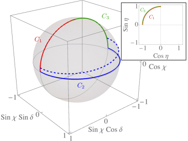
Figure 3: $\tilde{S}(\epsilon)$ along the braiding cycle. The color codes identifies the segments of the loop in parameter space depicted in Fig. 2. Here $\Gamma_{L}/\Gamma_{R}=0.3$, $\epsilon/\Gamma_{R}=0.01$ (solid curve) and $\epsilon/\Gamma_{R}=0.1$ (dashed curve). The inset shows a plot of the $U(1)$ phase of the scattering matrix, $\eta$, for general $\Gamma_{L}/\Gamma_{R}=0.3$ and $\epsilon/\Gamma_{R}=1\times 10^{-3}.$ (the two curves are shifted for clarity, the blue segment is not visible since $\eta$ is not affected)

.

Pumped charge and heat —

In order to identify a suitable transport property which reflects the global geometric properties of the path in parameter space (cf. Fig.2), we consider first the charge and heat current at lead $\alpha$, $I_{e,\alpha}=e/h\int d\epsilon[f_{\rm in}(\epsilon)-f_{\rm out}](\epsilon)$ and $I_{\epsilon,\alpha}=1/h\int d\epsilon(\epsilon-\mu)[f_{\rm in}(\epsilon)-f_{\rm out}]$ respectively, where $f_{\rm in}(\epsilon)$ and $f_{\rm out}(\epsilon)$ are the ingoing and outgoing electronic energy distribution functions in the leads, kept at temperature $T$ and voltage bias $eV=\mu$. The latter is determined by the time dependent scattering matrix of the system. Following a well established procedure Moskalets and Büttiker (2002), the scattering matrix is expanded to include the leading small slow-varying corrections, to obtain the expression for the pumped charge and heat $\mathcal{Q}_{e(\epsilon),\alpha}=\int_{0}^{\tau}dt\,I_{e(\epsilon),\alpha}(t)$ in terms of the parametric dependence of the scattering matrix Brouwer (1998). The result are known for the case superconducting leadsMoskalets and Büttiker (2002); Blaauboer (2002); Taddei et al. (2004), and we extend them here to a normal-superconducting junction with a Majorana zero modes – see sup .

At finite bias $\mu\neq 0$, the braiding manipulation gives rise to heat and charge currents, both accompanied by time-independent contributions. However, at $\mu=0$, as a direct consequence of particle-hole symmetry of the Majorana-lead coupling, the charge current is identically zero even in the presence of a driving. That is not generally the case for the heat current, which embeds the geometrical contribution resulting from the braiding protocol. In this limit, the heat pumping is given by $\mathcal{Q}_{\epsilon,\alpha}(\mu=0,T)=\int_{0}^{\tau}dt\,I_{\epsilon,\alpha}=2\int_{0}^{\infty}d\epsilon\,\epsilon\,\mathcal{Q}_{0,\alpha}(\epsilon)\partial f(\epsilon)/\partial\epsilon$ with

$$\mathcal{Q}_{0,\alpha}(\epsilon)=\oint_{C}\left(\frac{dn(\alpha)}{d\theta}d\theta+\frac{dn(\alpha)}{d\phi}d\phi\right),$$ (7)

where $f(\epsilon)$ is the Fermi distribution function and

$$\frac{dn(\alpha)}{dX} = \frac{1}{2\pi}\sum_{\beta,\nu}{\rm Im}\frac{\partial S^{e,\nu}_{\alpha,\beta}}{\partial X}{S^{e,\nu}_{\alpha,\beta}}^{*}$$ (8)

$$= \frac{1}{4\pi}\sum_{r}{\rm Im}\frac{\partial\tilde{S}_{\alpha^{-},r}}{\partial X}\tilde{S}_{\alpha^{-},r}^{*}-\frac{1}{4\pi}{\rm Im}\frac{\partial\tilde{S}_{\alpha^{-},\alpha^{-}}}{\partial X}.$$

Here $\beta=L,R$, $\nu=e,h$ and $r=L^{-},R^{-}$. At low temperatures, $T\to 0$, this expression reduces to:

$$\frac{\mathcal{Q}_{\epsilon,L}}{T}=2\ln 2\,\lim_{\epsilon\to 0}{Q}_{0,L}(\epsilon)+\mathcal{O}(T).$$ (9)

The zero energy limit of $\mathcal{Q}_{0,\alpha}$ can be conveniently computed using the mapping of the path in parameter space to that in the scattering matrix space, portrayed in Fig. 3. In this limit, the heat pumped approaches a universal value independent on the coupling parameters $\Gamma_{L},\Gamma_{R}$. Form Eq. (5) and Eq. (7) we find:

$$\frac{\mathcal{Q}_{\epsilon,L}}{2\ln 2\,T}=\frac{1}{4}$$ (10)

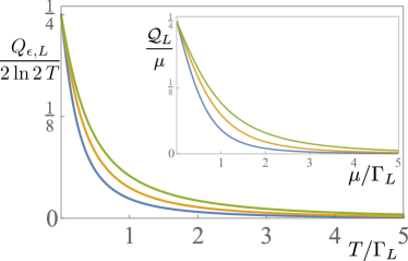
Figure 4: The heat pumped into the left lead during a braiding process, $\frac{\mathcal{Q}_{\epsilon,L}}{2\ln 2\,T}$, as a function of the temperature $T/\Gamma_{L}$. Different curves correspond to different values of the coupling $\Gamma_{R}/\Gamma_{L}=1$ (blue curve), $\Gamma_{R}/\Gamma_{L}=2$ (yellow curve), $\Gamma_{R}/\Gamma_{L}=4$ (Green curve). Inset shows the combined current and heat pumped during a braiding process as a function of the chemical potential $\mu/\Gamma_{L}$ at zero temperature, for different values of the coupling constants (same color code).

Eq. (10) is the main result of our paper. A few comments are in place. We first note that the braiding protocol defines a path in parameter space (see Fig. 2). At low scattering energies $\epsilon\to 0$ this path is mapped onto a distinctive path in the scattering matrix space, independent on the coupling to leads, which in turns leads to the universal value of $\mathcal{Q}_{\epsilon,\alpha}/T$. This universal value is therefore inherited from the geometrical properties of the path in parameter space, and reflects its topological protection, i.e. the measured heat pumped is protected against fluctuations of the coupling and the cycle driving. Second, in the absence of Majorana zero energy excitations, the ground state degeneracy is lifted. This corresponds to setting $\epsilon=0$ in Eqs. (5,Adiabatic change of scattering matrix —), where the path in parameter space would be trivial and there would be no pumped charge or heat. Finally, we see from Eq. (8) that $\mathcal{Q}_{\epsilon,R}=-\mathcal{Q}_{\epsilon,L}$. This anti-correlation of pumped heat at the two leads is distinctive of the Majorana braiding cycle, and can be used to distinguish the presence of Majorana bound states from a local zero energy Andreev bound state, which would generically result in uncorrelated heat transfer at the two leads.

The value of the pumped heat $\mathcal{Q}_{\epsilon,\alpha}$, is plotted as a function of $T$ in Fig. 4. The universal value $\mathcal{Q}_{\epsilon,\alpha}/2\ln 2\,T=1/4$ is obtained under the physical conditions $T\ll\mu\ll\min\{\Gamma_{L},\Gamma_{R}\}$. Away from this limit, at finite $T$, the pumped heat deviates form the universal value in a parameter dependent fashion. Applying a finite bias $\mu$, introduces time-independent contributions to the charge and heat currents which originate from Andreev reflection processes, present also in the absence of the adiabatic manipulation. In this case, the combination that singles out the contribution from the braiding process is $\mathcal{Q}_{\alpha}\equiv\mathcal{Q}_{\epsilon,\alpha}+\frac{\mu}{e}\mathcal{Q}_{e,\alpha}$ expressed by:

$$\mathcal{Q}_{\alpha}=\int_{0}^{\infty}d\epsilon\,\epsilon\,\mathcal{Q}_{0,\alpha}(\epsilon)\left[\frac{\partial f(\epsilon-\mu)}{\partial\epsilon}+\frac{\partial f(\epsilon+\mu)}{\partial\epsilon}\right],$$ (11)

with $\mathcal{Q}_{0,\alpha}$ given by Eq. (7). As long as $\mu\ll T$, a finite bias induces small corrections of the universal value. When $T\ll\mu$, instead, we have a different picture and a finite value of $\mathcal{Q}_{\alpha}$ is induced by the finite chemical potential. In the limit $T=0$, and $\mu\to 0$ we have

$$\frac{\mathcal{Q}_{L}}{\mu}=\lim_{\epsilon\to 0}\mathcal{Q}_{0,L}(\epsilon)=\frac{1}{4}$$ (12)

Here the role of temperature is replaced by the chemical potential. The non abelian phase acquired during the pumping cycle is embedded in the linear dependence on the pumped heat on chemical potential. The general dependence on the bias $\mu$ is shown in the inset of Fig. 4. As in the limit of $\mu=0$ and finite temperature, the deviation from the universal value occurs at $\mu\sim\min\{\Gamma_{L},\Gamma_{R}\}$.

Three-terminal geometry —

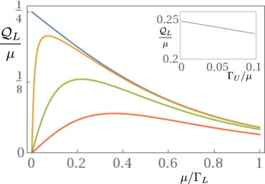
Figure 5: The differential heat per energy pumped into the left lead during a braiding process in the three lead configuration. Plots where calculated for $\Gamma_{L}/\Gamma_{R}=1$ and different coupling of the third lead $\Gamma_{U}/\Gamma_{L}=0$ (blue curve), $\Gamma_{U}/\Gamma_{L}=0.01$ (yellow curve), $\Gamma_{U}/\Gamma_{L}=0.1$ (Green curve) and $\Gamma_{U}/\Gamma_{L}=0.3$ (red curve). Inset shows the differential heat pumped into the left lead as a function of the ratio $\Gamma_{U}/\mu$. Here $\Gamma_{L}/\Gamma_{R}=0.3$ and $\mu/\Gamma_{L}=0.01$.

We next study the case where the three arms of the Y-junction setup are coupled to leads. This is described by the Hamiltonian $H=H_{Y}+H_{3T}+\sum_{\alpha}H_{\alpha}$ with the same notation as in the two-leads case and where $H_{3T}=H_{T}+t_{U}\left(c_{Uk}-c_{Uk}^{\dagger}\right)\gamma_{z}$ and $\alpha=L,R,U$. Following the steps outlined above, we calculate the scattering matrix using Eq. (3). In the rotated basis: $\tilde{\Psi}=(\Phi_{L}^{+},\Phi_{R}^{+},\Phi_{U}^{+},\Phi_{L}^{-},\Phi_{R}^{-},\Phi_{U}^{-})$ where $\Phi_{\alpha}^{\pm}=\frac{1}{\sqrt{2}}\left[\Phi_{e,\alpha}\pm\Phi_{h,\alpha}\right]$, the scattering matrix takes a block diagonal form, $S(\epsilon)=\mathbf{1}_{3}\oplus\tilde{S}(\epsilon)$, with $\tilde{S}(\epsilon)\in U(3)$. Restricting to the three dimensional basis of coupled channels, $\psi=(\Phi_{L}^{-},\Phi_{R}^{-},\Phi_{U}^{-})$ and projecting onto the ground state manifold, the coupling matrix takes the form $P_{\rm g}W=\sqrt{2}t_{L}\left[\cos\theta\cos\phi|\theta\rangle\langle L^{-}|-\sin\phi|\phi\rangle\langle L^{-}|\right]+\sqrt{2}t_{R}\left[\cos\theta\sin\phi|\theta\rangle\langle R^{-}|+\cos\phi|\phi\rangle\langle R^{-}|\right]+\sqrt{2}t_{U}\left[\sin\theta|\theta\rangle\langle U^{-}|\right]$

In the three terminal geometry, $\tilde{S}(\epsilon)$ takes a more complicated form than that in Eq. (5)(cf. Ref. [sup, ] for details). The combined heat and charge pumped along the cycle is then calculated using Eq. (7). Fig. 5 depicts the combined heat and charge, $Q_{L}/\mu$ pumped during a braiding process for different values of the coupling strength to the upper lead. Interestingly, the universal value at vanishing energy is lost once the broadening due to the coupling to the third lead is of the order of $\mu$. Therefore $\mathcal{Q}_{L}/\mu$ approaches $1/4$ only in the regime $\Gamma_{U}\ll\mu\ll\min{\Gamma_{R},\Gamma_{L}}$. This result is to be expected, as the limit $\mu\ll\min{\Gamma_{U},\Gamma_{L},\Gamma_{R}}$ is adiabatically connected to the limit of equal coupling, where we expect no charge transfer as a result of symmetry.

Conclusions–

In conclusion, we have analysed a quantum device in which Majorana zero modes undergo a dynamical braiding operation, while the system is continuously probed by external leads. Considering explicitly the implementation in superconducting nanostructures where two Majorana end-states are contacted to external leads, we have related the accumulated non-abelian geometric phase to a surface integral in the space of scattering matrices. In the limit of low energy, this results in a universal value of the heat density pumped during a cycle. (Notably, the pumped charge is identically zero). We have analysed the robustness of the effect against the variation of parameters, temperature, and setup geometry. Our results establishes a first connection between transport properties and topologically protected dynamical operations in Majorana based devices. The identified universal property can provide a new ingredient for engineering heat pumping devices and for understanding the role of topological protection in thermodynamic processes.

Acknowledgements–

We acknowledge discussions with Piet Brouwer, Dimitri Gutman, Tami Pereg-Barnea, and Janine Splettstösser. A.R. acknowledges support by EPSRC via Grant No. EP/P010180/1. D. M. acknowledges support from the Israel Science Foundation (Grant No. 737/14) and from the People Programme (Marie Curie Actions) of the European Union’s Seventh Framework Programme (FP7/2007-2013) under REA grant agreement No. 631064.

Part I Supplementary Materials

Here we present the derivation of the general form of the scattering matrix for the geometry with 2 and 3 contact leads. We derive a general formulas for pumped heat and charge for a system consisting of both superconducting and normal leads and apply it to the device considered in the paper.

I General form of the scattering matrix for 2 and 3 leads

We study first the case where we couple the superconducting Island to 3 leads. The setup is described by the Hamiltonian:

$$H_{0} = 2i\gamma_{0}\vec{\Delta}\cdot\vec{\gamma}$$

$$H_{T} = t_{L}\left(c_{Lk}-c_{Lk}^{\dagger}\right)\gamma_{x}+t_{R}\left(c_{Rk}-c_{Rk}^{\dagger}\right)\gamma_{y}+t_{U}\left(c_{Uk}-c_{Uk}^{\dagger}\right)\gamma_{z}$$

$$H_{\alpha} = \sum_{k}\xi_{k}c_{\alpha k}^{\dagger}c_{\alpha k}$$

Analogously to the procedure in the paper, we calculate the unitary scattering matrix: $\Psi_{\rm out}(\epsilon)=S(\epsilon)\Psi_{\rm in}(\epsilon)$ where the scattering states $\Psi_{\rm in}=(\Phi_{e,L},\Phi_{h,L},\Phi_{e,R},\Phi_{h,R},\Phi_{e,U},\Phi_{h,U})$ are in the basis of electrons $(e)$ and holes $(h)$ in the left and right leads. The scattering matrix can be expressed as:

$$S(\epsilon)=\openone+2\pi iW^{\dagger}\left(H_{0}-\epsilon-i\pi WW^{\dagger}\right)^{-1}W$$ (S1)

Where $W$ is the matrix that encodes the coupling to the leads. It is possible to perform a unitary transformation that decouples some of the leads degrees of freedom form the system. We work in this rotated basis defined by $\tilde{\Psi}=(\Phi_{L}^{+},\Phi_{R}^{+},\Phi_{U}^{+},\Phi_{L}^{-},\Phi_{R}^{-},\Phi_{U}^{-})$ where $\Phi_{\alpha}^{\pm}=\frac{1}{\sqrt{2}}\left[\Phi_{e,\alpha}\pm\Phi_{h,\alpha}\right]$. It follows directly that From Eq. (I) that, in this basis, the scattering matrix takes a block diagonal form with only three channels coupled to the dot. We therefore restrict to the three dimensional basis of coupled channels, namely $\psi=(\Phi_{L}^{-},\Phi_{R}^{-},\Phi_{U}^{-})$ . Denoting $\Gamma_{U}$ the coupling to the third lead, the coupling matrix takes the form:

$$W = \left(\begin{array}[]{cccc}\sqrt{\Gamma_{L}}&0&0\\ 0&\sqrt{\Gamma_{R}}&0\\ 0&0&\sqrt{\Gamma_{U}}\\ 0&0&0\end{array}\right)=\sqrt{\Gamma_{L}}|x\rangle\langle L^{-}|+\sqrt{\Gamma_{R}}|y\rangle\langle R^{-}|+\sqrt{\Gamma_{U}}|z\rangle\langle U^{-}|$$ (S6)

Projecting onto the ground state manifold: $P_{\rm g}=|\theta\rangle\langle\theta|+|\phi\rangle\langle\phi|$. We can write:

$$P_{\rm g}W = \sqrt{\Gamma_{L}}\left[\langle\theta|x\rangle|\theta\rangle\langle L^{-}|+\langle\phi|x\rangle|\phi\rangle\langle L^{-}|\right]+\sqrt{\Gamma_{R}}\left[\langle\theta|y\rangle|\theta\rangle\langle R^{-}|+\langle\phi|y\rangle|\phi\rangle\langle R^{-}|\right]+\sqrt{\Gamma_{U}}\left[\langle\theta|z\rangle|\theta\rangle\langle U^{-}|+\langle\phi|z\rangle|\phi\rangle\langle U^{-}|\right]$$ (S7)

$$= \sqrt{\Gamma_{L}}\left[\cos\theta\cos\phi|\theta\rangle\langle L^{-}|-\sin\phi|\phi\rangle\langle L^{-}|\right]+\sqrt{\Gamma_{R}}\left[\cos\theta\sin\phi|\theta\rangle\langle R^{-}|+\cos\phi|\phi\rangle\langle R^{-}|\right]-\sqrt{\Gamma_{U}}\left[\sin\theta|\theta\rangle\langle U^{-}|\right]$$

The non-trivial part of the scattering matrix follows:

$$\tilde{S}(\epsilon) = \openone+2iW^{\dagger}\left(P_{\rm g}[H_{0}-\epsilon-iWW^{\dagger}]P_{\rm g}\right)^{-1}W$$ (S8)

$$= \openone-2iW^{\dagger}\left(\epsilon+iP_{\rm g}WW^{\dagger}P_{\rm g}\right)^{-1}W$$

$$= |L^{-}\rangle\langle L^{-}|\left\{1-2i\Gamma_{L}\left[\frac{\left(\epsilon+i\Gamma_{R}\right)\cos^{2}\theta+\left(\epsilon+i\Gamma_{U}\right)\sin^{2}\theta\sin^{2}\phi}{\left(\epsilon+i\Gamma_{U}\right)\sin^{2}\theta\left(\epsilon+i\Gamma_{L}\sin^{2}\phi+i\Gamma_{R}\cos^{2}\phi\right)+\left(\epsilon+i\Gamma_{L}\right)\left(\epsilon+i\Gamma_{R}\right)\cos^{2}\theta}\right]\right\}$$

$$+ |R^{-}\rangle\langle R^{-}|\left\{1-2i\Gamma_{R}\left[\frac{\left(\epsilon+i\Gamma_{L}\right)\cos^{2}\theta+\left(\epsilon+i\Gamma_{U}\right)\sin^{2}\theta\cos^{2}\phi}{\left(\epsilon+i\Gamma_{U}\right)\sin^{2}\theta\left(\epsilon+i\Gamma_{L}\sin^{2}\phi+i\Gamma_{R}\cos^{2}\phi\right)+\left(\epsilon+i\Gamma_{L}\right)\left(\epsilon+i\Gamma_{R}\right)\cos^{2}\theta}\right]\right\}$$

$$+ |U^{-}\rangle\langle U^{-}|\left\{1-2i\Gamma_{U}\sin^{2}\theta\left[\frac{\left(\epsilon+i\Gamma_{L}\sin^{2}\phi+i\Gamma_{R}\cos^{2}\phi\right)}{\left(\epsilon+i\Gamma_{U}\right)\sin^{2}\theta\left(\epsilon+i\Gamma_{L}\sin^{2}\phi+i\Gamma_{R}\cos^{2}\phi\right)+\left(\epsilon+i\Gamma_{L}\right)\left(\epsilon+i\Gamma_{R}\right)\cos^{2}\theta}\right]\right\}$$

$$- 2i\sqrt{\Gamma_{L}\Gamma_{R}}\left[|L^{-}\rangle\langle R^{-}|+|R^{-}\rangle\langle L^{-}|\right]\left\{\frac{\left(\epsilon+i\Gamma_{U}\right)\sin^{2}\theta\cos\phi\sin\phi}{\left(\epsilon+i\Gamma_{U}\right)\sin^{2}\theta\left(\epsilon+i\Gamma_{L}\sin^{2}\phi+i\Gamma_{R}\cos^{2}\phi\right)+\left(\epsilon+i\Gamma_{L}\right)\left(\epsilon+i\Gamma_{R}\right)\cos^{2}\theta}\right\}$$

$$+ 2i\sqrt{\Gamma_{U}\Gamma_{R}}\left[|U^{-}\rangle\langle R^{-}|+|R^{-}\rangle\langle U^{-}|\right]\left\{\frac{\left(\epsilon+i\Gamma_{L}\right)\cos\phi\cos\theta\sin\theta}{\left(\epsilon+i\Gamma_{U}\right)\sin^{2}\theta\left(\epsilon+i\Gamma_{L}\sin^{2}\phi+i\Gamma_{R}\cos^{2}\phi\right)+\left(\epsilon+i\Gamma_{L}\right)\left(\epsilon+i\Gamma_{R}\right)\cos^{2}\theta}\right\}$$

$$+ 2i\sqrt{\Gamma_{U}\Gamma_{L}}\left[|U^{-}\rangle\langle L^{-}|+|L^{-}\rangle\langle U^{-}|\right]\left\{\frac{\left(\epsilon+i\Gamma_{R}\right)\sin\phi\cos\theta\sin\theta}{\left(\epsilon+i\Gamma_{U}\right)\sin^{2}\theta\left(\epsilon+i\Gamma_{L}\sin^{2}\phi+i\Gamma_{R}\cos^{2}\phi\right)+\left(\epsilon+i\Gamma_{L}\right)\left(\epsilon+i\Gamma_{R}\right)\cos^{2}\theta}\right\}\$$

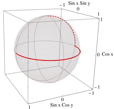
Figure S1: The evolution the $x$ and $y$ angles of the scattering matrix, Eq. (I) during the first segment of the pumping cycle. The solid line was calculated for $\Gamma_{U}/\Gamma_{L}=0.3$ and $\epsilon/\Gamma_{L}=10^{-4}$, while the dashed line shows the limit of uncoupling the upper lead$\Gamma_{L}\gg\epsilon\gg\Gamma_{U}$, where $\epsilon/\Gamma_{L}=10^{-2}$ and $\Gamma_{U}/\Gamma_{L}=10^{-5}$.

The expression in Eq. (S8) simplifies considerably when the scattering matrix is evaluated along the path in parameter space of the pumping cycle. We obtain, for the three branches of the cycle:

$$S(\mathcal{C}_{1}) = e^{-ix_{\vec{C}_{1}}}\left[\cos x_{\vec{C}_{1}}\frac{4\mathbf{1}+3\lambda_{3}-\sqrt{3}\lambda_{8}}{6}+i\sin x_{\vec{C}_{1}}\cos y_{\vec{C}_{1}}\frac{\sqrt{3}\lambda_{8}+\lambda_{3}}{2}+i\sin x_{\vec{C}_{1}}\sin y_{\vec{C}_{1}}\lambda_{4}\right]+e^{-2i\zeta_{R}}\frac{2\mathbf{1}-3\lambda_{3}+\sqrt{3}\lambda_{8}}{6}$$

$$S(\mathcal{C}_{2}) = e^{-ix_{\vec{C}_{2}}}\left[\cos x_{\vec{C}_{2}}\frac{2\mathbf{1}+\sqrt{3}\lambda_{8}}{3}+i\sin x_{\vec{C}_{2}}\cos y_{\vec{C}_{2}}\lambda_{3}+i\sin x_{\vec{C}_{2}}\sin y_{\vec{C}_{2}}\lambda_{1}\right]+e^{-2i\zeta_{U}}\frac{\mathbf{1}-\sqrt{3}\lambda_{8}}{3}$$

$$S(\mathcal{C}_{3}) = e^{-ix_{\vec{C}_{3}}}\left[\cos x_{\vec{C}_{3}}\frac{4\mathbf{1}-3\lambda_{3}-\sqrt{3}\lambda_{8}}{6}+i\sin x_{\vec{C}_{3}}\cos y_{\vec{C}_{3}}\frac{1}{2}\left[\sqrt{3}\lambda_{8}-\lambda_{3}\right]+i\sin x_{\vec{C}_{3}}\sin y_{\vec{C}_{3}}\lambda_{6}\right]+e^{-2i\zeta_{L}}\frac{2\mathbf{1}+3\lambda_{3}+\sqrt{3}\lambda_{8}}{6}$$

where $\vec{C}_{1}=(L,U,\theta)$, $\vec{C}_{2}=(R,L,\phi)$, $\vec{C}_{3}=\vec{C}_{3}=(U,R,\phi)$ and $\tan x_{(\alpha,\beta,\psi)}=(\Gamma_{\alpha}\cos\psi^{2}+\Gamma_{\beta}\sin\psi^{2})/\epsilon$, $\tan y_{(\alpha,\beta,\psi)}=(2\sqrt{\Gamma_{\alpha}\Gamma_{\beta}}\cos\psi\sin\psi)/(\Gamma_{\beta}\sin\psi^{2}-\Gamma_{\alpha}\cos\psi^{2})$ and $\tan\zeta_{\alpha}=\Gamma_{\alpha}/\epsilon$. The scattering matrix dependence on the parameters is represented graphically in Fig. S1, which presents the $x$ and $y$ components along the path in parameter space.

II General form of the Scattering matrix for 2 leads

Upon decoupling one of the leads, by setting $\Gamma_{U}=0$ in Eq. (S8), the scattering matrix reduces to that of the two-leads geometry, $\tilde{S}(\epsilon)\in SU(2)$, which can be parametrised in terms of scattering matrices as

$$\tilde{S}(\epsilon)=e^{-i\eta(\epsilon)}e^{-i\chi(\epsilon)\left(\cos\delta(\epsilon)\sigma_{z}+\sin\delta(\epsilon)\sigma_{x}\right)}=e^{-i\eta(\epsilon)}\left[\cos\chi(\epsilon)-i\sin\chi(\epsilon)\left(\cos\delta(\epsilon)\sigma_{z}+\sin\delta(\epsilon)\sigma_{x}\right)\right]$$

with

$$\tan\delta(\epsilon) = \frac{2\sqrt{\Gamma_{L}\Gamma_{R}}\sin\theta^{2}\sin 2\phi}{(\Gamma_{L}-\Gamma_{R})(1+\cos\theta^{2})-(\Gamma_{L}+\Gamma_{R})(\sin\theta^{2}\cos 2\phi)}\xrightarrow[]{\Gamma_{L}\rightarrow\Gamma_{R}}\tan 2\phi$$

$$\tan\chi(\epsilon) = \frac{\epsilon\sqrt{\left[(\Gamma_{L}-\Gamma_{R})(1+\cos\theta^{2})-(\Gamma_{L}+\Gamma_{R})(\sin\theta^{2}\cos 2\phi)\right]^{2}+4\Gamma_{L}\Gamma_{R}\sin\theta^{4}\sin 2\phi^{2}}}{2\left[\epsilon^{2}+\Gamma_{L}\Gamma_{R}\cos\theta^{2}\right]}\xrightarrow[]{\Gamma_{L}\rightarrow\Gamma_{R}}\frac{\epsilon\Gamma\sin\theta^{2}}{\epsilon^{2}+\Gamma^{2}\cos\theta^{2}}$$

$$\tan\eta(\epsilon) = \frac{\epsilon\left[\Gamma_{L}(\cos\theta^{2}+\sin\theta^{2}\sin\phi^{2})+\Gamma_{R}(\cos\theta^{2}+\sin\theta^{2}\cos\phi^{2})\right]}{\epsilon^{2}-\Gamma_{L}\Gamma_{R}\cos\theta^{2}}\xrightarrow[]{\Gamma_{L}\rightarrow\Gamma_{R}}\frac{\epsilon\Gamma(1+\cos\theta^{2})}{\epsilon^{2}-\Gamma^{2}\cos\theta^{2}}$$ (S9)

In the limit of equal coupling we recover the simplified expressions (6) in the paper.

III Pumped charge and heat with normal and superconducting leads

The main result of the paper establishes a relation between the geometric phases associated with the braiding of Majorana zero modes and transport across the system. Specifically the pumped heat across the cycle encodes informations on the geometric phase. We derive here the general expression for the pumped charge and heat in setups consisting of both normal and superconducting leads, and use it for the Majorana-based device studied in the paper.

The starting point for our derivation are the results obtained for charge pumping Moskalets and Büttiker (2002); Blaauboer (2002); Taddei et al. (2004). The system under consideration consists of $N$ normal leads contacted to a mesocopic device in the presence of a grounded superconductor. The amplitude for electrons and holes injected from lead $\alpha$ to be reflected /transmitted as electrons or holes at lead $\beta$ is determined by the scattering matrix $S_{\beta,\alpha}^{(ij)}(t)$, where $i,j\in\{e,h\}$, with the same notation used in the paper. The outgoing charge and energy currents at lead $\alpha$ are given by

$$I_{e,\alpha} = \frac{e}{h}\int_{0}^{\infty}dE\left[f_{{\rm out},\alpha}(E)-f_{{\rm in},\alpha}(E)\right],$$ (S10)

$$I_{\epsilon,\alpha} = \frac{1}{h}\int_{0}^{\infty}dE(E-\mu_{\alpha})\left[f_{{\rm out},\alpha}(E)-f_{{\rm in},\alpha}(E)\right],$$ (S11)

Here the distribution of the ingoing particles at lead $\alpha$ is the equilibrium distribution set by the external temperature and chemical potential, $f_{{\rm in},\alpha}(E)=f_{0}(E-\mu_{\alpha})$, and the outgoing one is determined by the scattering properties of the systems.

In the following we simplify $\left[f_{{\rm out},\alpha}(E)-f_{{\rm in},\alpha}(E)\right]$, and the result can be used for both the charge and heat current. We assume that all the leads are kept at the same chemical potential, $\mu_{\alpha}=\mu$. Moreover, the time dependence of the scattering matrix on time is due to the weak slow periodic driving of external parameters, $X_{j}(t)=X_{j}+X_{j,\omega}e^{i(\omega t-\phi_{j})}+X_{j,\omega}e^{-i(\omega t-\phi_{j})}$. The time-dependence of the scattering matrix is then expressed given by

$$\hat{S}(t)=\hat{S}+\hat{S}_{\omega}e^{-i\omega t}+\hat{S}_{-\omega}e^{i\omega t},$$ (S12)

with

$$\hat{S}_{\pm\omega}=\sum_{j}X_{j,\omega}e^{\mp i\phi_{j}}\frac{\partial\hat{S}}{\partial X_{j}}.$$ (S13)

This essentially corresponds to including the scattering process involving the nearest energy side-bands. The distribution of outgoing electrons at energy $E$ is therefore determined by the distribution of ingoing electrons and holes at energies $E$, $E+\omega$ and $E-\omega$. With the observation that the ingoing equilibrium distribution of holes is given by $f^{(h)}_{{\rm in},\beta}(E)=f_{0}(E+\mu)$, we get

$$f_{{\rm out},\alpha}(E)=\sum_{\beta} \left[|S_{\alpha,\beta}^{ee}|^{2}f_{0}(E-\mu)+|S_{-\omega,\alpha,\beta}^{ee}|^{2}f_{0}(E-\mu+\omega)+|S_{\omega,\alpha,\beta}^{ee}|^{2}f_{0}(E-\mu-\omega)\right.$$ (S14)

$$\left.+|S_{\alpha,\beta}^{eh}|^{2}f_{0}(E+\mu)+|S_{-\omega,\alpha,\beta}^{eh}|^{2}f_{0}(E+\mu+\omega)+|S_{\omega,\alpha,\beta}^{eh}|^{2}f_{0}(E+\mu-\omega)\right].$$

Expanding Eq. (S14) at leading order in $\omega\to 0$, and using the unitarity of the scattering matrix, $\left(\hat{S}+\hat{S}_{\omega}e^{-i\omega t}+\hat{S}_{-\omega}e^{i\omega t}\right)\cdot\left(\hat{S}^{\dagger}+\hat{S}^{\dagger}_{\omega}e^{+i\omega t}+\hat{S}^{\dagger}_{-\omega}e^{-i\omega t}\right)=1$, we get

$$I_{e,\alpha} = \frac{e}{h}\int_{-\infty}^{\infty}dE\left[\left(f_{0}(E+\mu)-f_{0}(E-\mu)\right)\left(1-|S_{\alpha,\beta}^{ee}|^{2}-|S_{\omega,\alpha,\beta}^{ee}|^{2}-|S_{-\omega,\alpha,\beta}^{ee}|^{2}\right)\phantom{\frac{a}{b}}\right.$$ (S15)

$$\left.+\hbar\omega\frac{\partial f(E-\mu)}{\partial E}\left(|S_{-\omega,\alpha,\beta}^{ee}|^{2}-|S_{\omega,\alpha,\beta}^{ee}|^{2}\right)+\hbar\omega\frac{\partial f(E+\mu)}{\partial E}\left(|S_{-\omega,\alpha,\beta}^{eh}|^{2}-|S_{\omega,\alpha,\beta}^{eh}|^{2}\right),\right]$$

and

$$I_{\epsilon,\alpha} = \frac{1}{h}\int_{-\infty}^{\infty}dE(E-\mu)\left[\left(f_{0}(E+\mu)-f_{0}(E-\mu)\right)\left(1-|S_{\alpha,\beta}^{ee}|^{2}-|S_{\omega,\alpha,\beta}^{ee}|^{2}-|S_{-\omega,\alpha,\beta}^{ee}|^{2}\right)\phantom{\frac{a}{b}}\right.$$ (S16)

$$\left.+\hbar\omega\frac{\partial f(E-\mu)}{\partial E}\left(|S_{-\omega,\alpha,\beta}^{ee}|^{2}-|S_{\omega,\alpha,\beta}^{ee}|^{2}\right)+\hbar\omega\frac{\partial f(E+\mu)}{\partial E}\left(|S_{-\omega,\alpha,\beta}^{eh}|^{2}-|S_{\omega,\alpha,\beta}^{eh}|^{2}\right)\right],$$

where we have shifted the energy to be measured from the superconductor chemical potential and we have neglected the effect of finite band size in extending the integral over all energies.

The expressions for $I_{e}$ and $I_{\epsilon}$ can be simplified using the symmetries of the scattering matrix. In fact, $S^{ee}_{\alpha,\beta}(-E)=\left(S^{ee}_{\alpha,\beta}(E)\right)^{*}$, and as a consequence:

$$1-|S_{\alpha,\beta}^{ee}(-E)|^{2}-|S_{\omega,\alpha,\beta}^{ee}(-E)|^{2}-|S_{-\omega,\alpha,\beta}^{ee}(-E)|^{2}=1-|S_{\alpha,\beta}^{ee}(E)|^{2}-|S_{\omega,\alpha,\beta}^{ee}(E)|^{2}-|S_{-\omega,\alpha,\beta}^{ee}(E)|^{2}$$

$$T^{ee}_{\alpha,\beta}(-E)\equiv|S_{-\omega,\alpha,\beta}^{ee}(-E)|^{2}-|S_{\omega,\alpha,\beta}^{ee}(-E)|^{2}=-|S_{-\omega,\alpha,\beta}^{ee}(E)|^{2}-|S_{\omega,\alpha,\beta}^{ee}(E)|^{2}=-T^{ee}_{\alpha,\beta}(E)$$

$$T^{eh}_{\alpha,\beta}(-E)\equiv|S_{-\omega,\alpha,\beta}^{eh}(-E)|^{2}-|S_{\omega,\alpha,\beta}^{eh}(-E)|^{2}=-|S_{-\omega,\alpha,\beta}^{eh}(E)|^{2}-|S_{\omega,\alpha,\beta}^{eh}(E)|^{2}=-T^{eh}_{\alpha,\beta}(E).$$ (S17)

Using the parity properties of the fermi function, we can therefore rewrite the heat and charge currents as integrals over positive energies only

$$I_{e,\alpha} = 2\int_{0}^{\infty}dE\,\left[\left(f_{0}(E+\mu)-f_{0}(E-\mu)\right)\left(1-|S_{\alpha,\beta}^{ee}(E)|^{2}-|S_{\omega,\alpha,\beta}^{ee}(E)|^{2}-|S_{-\omega,\alpha,\beta}^{ee}(E)|^{2}\right)\right]$$ (S18)

$$+\frac{e\omega}{2\pi}\sum_{\beta}\int_{0}^{\infty}dE\,\left[\frac{\partial f(E-\mu)}{\partial E}\left(T^{ee}_{\alpha,\beta}(E)-T^{eh}_{\alpha,\beta}(E)\right)+\frac{\partial f(E+\mu)}{\partial E}\left(T^{eh}_{\alpha,\beta}(E)-T^{ee}_{\alpha,\beta}(E)\right)\right],$$

$$I_{\epsilon,\alpha} = -\frac{\mu}{e}I_{e,\alpha}+\frac{\omega}{2\pi}\sum_{\beta}\int_{0}^{\infty}dE\,E\,\left[\frac{\partial f(E-\mu)}{\partial E}\left(T^{ee}_{\alpha,\beta}(E)+T^{eh}_{\alpha,\beta}(E)\right)+\frac{\partial f(E+\mu)}{\partial E}\left(T^{eh}_{\alpha,\beta}(E)+T^{ee}_{\alpha,\beta}(E)\right)\right].$$ (S19)

Note that at $\mu=0$ $I_{e,\alpha}=0$ identically. This is a consequence of the symmetry of the scattering matrix, and is in contrast with usual results for which the scattering matrix is approximated to be independent of energy. In that case the expressions in (III) are even under energy reversal and one has a vanishing heat current as opposed to a finite charge current.

The expressions can be further simplified by computing explicitly

$$\sum_{\beta=L,R}T^{ee}_{L,\beta}=\frac{1}{4}\delta X_{1}\delta X_{2}{\rm Im}\left[\frac{\partial S_{L-,L-}}{\partial X_{1}}\frac{\partial S_{L-,L-}^{*}}{\partial X_{2}}+\frac{\partial S_{L-,R-}}{\partial X_{1}}\frac{\partial S_{L-,R-}^{*}}{\partial X_{2}}\right]=\sum_{\beta=L,R}T^{eh}_{L,\beta},$$ (S20)

and similarly for $T^{ee}_{R,\beta}$. This leads to the expressions

$$I_{e,\alpha} = 2\int_{0}^{\infty}dE\,\left[\left(f_{0}(E+\mu)-f_{0}(E-\mu)\right)\left(1-|S_{\alpha,\beta}^{ee}(E)|^{2}-|S_{\omega,\alpha,\beta}^{ee}(E)|^{2}-|S_{-\omega,\alpha,\beta}^{ee}(E)|^{2}\right)\right],$$ (S21)

$$I_{\epsilon,\alpha} = -\frac{\mu}{e}I_{e,\alpha}+\frac{\omega}{\pi}\sum_{\beta}\int_{0}^{\infty}dE\,E\,\left[\frac{\partial f(E-\mu)}{\partial E}T^{ee}_{\alpha,\beta}(E)+\frac{\partial f(E+\mu)}{\partial E}T^{ee}_{\alpha,\beta}(E)\right],$$ (S22)

which appear in the manuscript. Note that the only time dependence enters through $X_{1}$ and $X_{2}$, and one can perform the time integral over the pumping cycle inside the energy integral. In particular we consider the combination $\mathcal{Q}_{\alpha}(\mu,T)=\int_{0}^{\tau}dt\,(I_{\epsilon,\alpha}+\mu I_{e,\alpha}/e)$, so that

$$\mathcal{Q}_{\alpha}(\mu,T)=\int_{0}^{\tau}dt\,(I_{\epsilon,\alpha}+\frac{\mu}{e}I_{e,\alpha})=\int_{0}^{\infty}dE\,E\,\mathcal{Q}_{0,\alpha}(E)\left[\frac{\partial f(E-\mu)}{\partial E}+\frac{\partial f(E+\mu)}{\partial E}\right].$$ (S23)

with

$$\mathcal{Q}_{0,\alpha}(E)=\frac{1}{\pi}\int_{A}dX_{1}dX_{2}\sum_{\beta=L,R,\nu=e,h}{\rm Im}\left[\frac{\partial S^{e\nu}_{\alpha,\beta}}{\partial X_{1}}\frac{\partial{S^{e\nu}_{\alpha,\beta}}^{*}}{\partial X_{2}}\right]=\int_{0}^{\tau}dt\left(\frac{dn(\alpha)}{dX_{1}}\frac{dX_{1}}{dt}+\frac{dn(\alpha)}{dX_{2}}\frac{dX_{2}}{dt}\right)$$ (S24)

and

$$\frac{dn(\alpha)}{dX}=\frac{1}{2\pi}\sum_{\beta=L,R,\nu=e,h}{\rm Im}\frac{\partial S^{e\nu}_{\alpha,\beta}}{\partial X}{S^{e\nu}_{\alpha,\beta}}^{*}$$ (S25)

Note that at $T=0$ $\mathcal{Q}_{L}(\mu,0)=\mathcal{Q}(\mu)$, which, for $\mu\to 0$ approaches the universal fraction of the solid angle discussed in the manuscript.

References

• Wilczek (1982) F. Wilczek, Phys. Rev. Lett. 49, 957 (1982).
• Read and Green (2000) N. Read and D. Green, Phys. Rev. B 61, 10267 (2000) .
• Stern (2010) A. Stern, Nature 464, 187 (2010).
• Nayak et al. (2008) C. Nayak, S. H. Simon, A. Stern, M. Freedman, and S. Das Sarma, Rev. Mod. Phys. 80, 1083 (2008) .
• Moore and Read (1991) G. Moore and N. Read, Nucl. Phys. B 360, 362 (1991).
• Kitaev (2001) A. Kitaev, Physics-Uspekhi 44, 16 (2001) .
• Fu and Kane (2008) L. Fu and C. L. Kane, Phys. Rev. Lett. 100, 096407 (2008) .
• Lutchyn et al. (2010) R. M. Lutchyn, J. D. Sau, and S. Das Sarma, Phys. Rev. Lett. 105, 077001 (2010) .
• Oreg et al. (2010) Y. Oreg, G. Refael, and F. von Oppen, Phys. Rev. Lett. 105, 177002 (2010) .
• Mourik et al. (2012) V. Mourik, K. Zuo, S. M. Frolov, S. R. Plissard, E. P. a. M. Bakkers, and L. P. Kouwenhoven, Science 336, 1003 (2012) .
• Das et al. (2012) A. Das, Y. Ronen, Y. Most, Y. Oreg, M. Heiblum, and H. Shtrikman, Nat. Phys. 8, 887 (2012) .
• Churchill et al. (2013) H. O. H. Churchill, V. Fatemi, K. Grove-Rasmussen, M. T. Deng, P. Caroff, H. Q. Xu, and C. M. Marcus, Phys. Rev. B 87, 241401 (2013) .
• Nadj-Perge et al. (2014) S. Nadj-Perge, I. K. Drozdov, J. Li, H. Chen, S. Jeon, J. Seo, A. H. MacDonald, B. A. Bernevig, and A. Yazdani, Science 346, 602 (2014) .
• Albrecht et al. (2016) S. M. Albrecht, A. P. Higginbotham, M. Madsen, F. Kuemmeth, T. S. Jespersen, J. Nygård, P. Krogstrup, and C. M. Marcus, Nature 531, 206 (2016) .
• Deng et al. (2016) M. T. Deng, S. Vaitiekėnas, E. B. Hansen, J. Danon, M. Leijnse, K. Flensberg, J. Nygård, P. Krogstrup, and C. M. Marcus, Science 354, 1557 (2016) .
• Aasen et al. (2016) D. Aasen, M. Hell, R. V. Mishmash, A. Higginbotham, J. Danon, M. Leijnse, T. S. Jespersen, J. A. Folk, C. M. Marcus, K. Flensberg, et al., Phys. Rev. X 6, 031016 (2016) .
• Plugge et al. (2016a) S. Plugge, L. A. Landau, E. Sela, A. Altland, K. Flensberg, and R. Egger, Phys. Rev. B 94, 174514 (2016) .
• Plugge et al. (2016b) S. Plugge, A. Rasmussen, R. Egger, and K. Flensberg, New J. Phys. 19, 012001 (2017) .
• Fu (2010) L. Fu, Phys. Rev. Lett. 104, 056402 (2010) .
• Michaeli et al. (2016) K. Michaeli, L. A. Landau, E. Sela, and L. Fu, Phys. Rev. B 96, 205403 (2017) .
• Vijay and Fu (2016) S. Vijay and L. Fu, Phys. Rev. B 94, 235446 (2016) .
• Zocher and Rosenow (2013) B. Zocher and B. Rosenow, Phys. Rev. Lett. 111, 036802 (2013) .
• Rubbert and Akhmerov (2016) S. Rubbert and A. R. Akhmerov, Phys. Rev. B 94, 115430 (2016).
• Romito and Gefen (2017) A. Romito and Y. Gefen, Phys. Rev. Lett. 119, 157702 (2017).
• Flensberg (2010) K. Flensberg, Phys. Rev. B 82, 180516 (2010).
• Bonderson et al. (2008) P. Bonderson, M. Freedman, and C. Nayak, Phys. Rev. Lett. 101, 010501 (2008) .
• Bonderson (2013) P. Bonderson, Phys. Rev. B 87, 035113 (2013) .
• Karzig et al. (2017) T. Karzig, C. Knapp, R. M. Lutchyn, P. Bonderson, M. B. Hastings, C. Nayak, J. Alicea, K. Flensberg, S. Plugge, Y. Oreg, et al., Phys. Rev. B 95, 235305 (2017) .
• Fulga et al. (2011) I. C. Fulga, F. Hassler, A. R. Akhmerov, and C. W. J. Beenakker, Phys. Rev. B 83, 155429 (2011)
• Meidan et al. (2014) D. Meidan, A. Romito, and P. W. Brouwer, Phys. Rev. Lett. 113, 057003 (2014)
• Meidan et al. (2016) D. Meidan, A. Romito, and P. W. Brouwer, Phys. Rev. B 93, 125433 (2016)
• van Heck et al. (2012) B. van Heck, a. R. Akhmerov, F. Hassler, M. Burrello, and C. W. J. Beenakker, New J. Physics 14, 035019 (2012)
• Karzig et al. (2016) T. Karzig, Y. Oreg, G. Refael, and M. H. Freedman, Physical Review X 6, 031019 (2016)
• (34) C. Mahaux and H. A. Weidenmüller, Shell-Model Approach to Nuclear Reactions (North-Holland, Amsterdam, 1969).
• Moskalets and Büttiker (2002) M. Moskalets and M. Büttiker, Phys. Rev. B 66, 035306 (2002)
• Brouwer (1998) P. W. Brouwer, Phys. Rev. B 58, R10135 (1998)
• Blaauboer (2002) M. Blaauboer, Phys. Rev. B 65, 235318 (2002)
• Taddei et al. (2004) F. Taddei, M. Governale, and R. Fazio, Phys. Rev. B 70, 052510 (2004).
• (39) See supplementary material.

References

• Moskalets and Büttiker (2002) M. Moskalets and M. Büttiker, Phys. Rev. B 66, 035306 (2002)
• Blaauboer (2002) M. Blaauboer, Phys. Rev. B 65, 1 (2002)
• Taddei et al. (2004) F. Taddei, M. Governale, and R. Fazio, Phys. Rev. B 70, 052510 (2004).