Constructing Binary Neutron Star Initial Data with
High Spins, High Compactness, and High Mass-Ratios

Abstract

The construction of accurate and consistent initial data for various binary parameters is a critical ingredient for numerical relativity simulations of the compact binary coalescence. In this article, we present an upgrade of the pseudospectral SGRID code, which enables us to access even larger regions of the binary neutron star parameter space. As a proof of principle, we present a selected set of first simulations based on initial configurations computed with the new code version. In particular, we simulate two millisecond pulsars close to their breakup spin, highly compact neutron stars with masses at about $98\%$ of the maximum supported mass of the employed equation of state, and an unequal mass systems with mass ratios even outside the range predicted by population synthesis models ($q=2.03$). The discussed code extension will help us to simulate previously unexplored binary configurations. This is a necessary step to construct and test new gravitational wave approximants and to interpret upcoming binary neutron star merger observations. When we construct initial data, one has to specify various parameters, such as a rotation parameter for each star. Some of these parameters do not have direct physical meaning, which makes comparisons with other methods or models difficult. To facilitate this, we introduce simple estimates for the initial spin, momentum, mass, and center of mass of each individual star.

I Introduction

In August 2017, the combined detection of a gravitational-wave (GW) signal and the detection of electromagnetic (EM) signals across the whole spectrum emitted from the same astrophysical source, a binary neutron star (BNS) merger, initiated a new era of multi-messenger astronomy Abbott et al. (2017a); Abbott et al. (2017b).

While there are analytical models to describe the BNS coalescence as long as the two stars are well separated, the highly non-linear regime around the moment of merger is only accessible with full numerical relativity (NR) simulations. These simulations allow us to study the dynamics, GW signal, and possible EM counterparts, and are therefore required for a true multi-messenger interpretation.

Most NR simulations are based on a 3+1-decomposition in which the 4-dimensional spacetime is foliated by spacelike hypersurfaces. This means that for a successful numerical simulation one has to solve the Einstein equations and the equations governing general relativistic matter on a spacelike hypersurface as an initial condition; see e.g., Cook (2000) or Tichy (2017) and references therein. Generally, these initial data have to provide configurations in which the stars are sufficiently far away from each other to allow a study of the emitted GW signal, but one also wants a distance short enough to avoid the computational cost of too many orbits. Current state-of-the-art BNS simulations reach from a few orbits up to 22 orbits prior to merger Haas et al. (2016).

Given the diversity of the BNS population, one has to be able to construct accurate initial data for a variety of different binary parameters for an accurate interpretation of future detections. As an example, even relatively small spins can, if neglected, lead to biases in the estimation of the source properties, e.g., Favata (2014); Agathos et al. (2015); Samajdar and Dietrich (2019). This fact together with the observation of a number of highly-spinning neutron stars (NS), e.g., PSR J1748$-$2446ad Hessels et al. (2006) (the fastest spinning NS, $716$ Hz), PSR J1807-2500B Lynch et al. (2012) (the fastest spinning NS in a binary, $239$ Hz), and PSR J1946+2052 Stovall et al. (2018) (the fastest spinning NS in a BNS system, $59$ Hz), make the accurate modelling of spin effects indispensable.

Similarly, the observation of massive NSs $m_{\rm NS}>2M_{\odot}$, e.g., PSR J0740+6620 (Cromartie et al., 2019) with $m=2.14^{+0.10}_{-0.09}$, shows that it is important to simulate stars with high mass and thus high compactness. Collisions of such massive stars might be almost indistinguishable from the merger of small black holes (BH), since the amount of the ejected material and consequently the brightness of the kilonova typically decrease for high compactnesses and larger total masses Dietrich and Ujevic (2017). Additional simulations are needed to further improve estimates of the prompt collapse threshold Bauswein et al. (2013); Köppel et al. (2019), i.e., the mass at which the colliding neutron stars immediately form a black hole. Such threshold mass estimates will become particularly important once the increasing number of GW triggers will no longer allow expensive EM follow-up campaigns for all potential GW candidates and thus observational overhead needs to be reduced.

Finally, as shown in, e.g., Hinderer et al. (2010); Dietrich et al. (2017a); Dietrich and Ujevic (2017); Lehner et al. (2016); Zappa et al. (2018); Kiuchi et al. (2019a) the mass-ratio of a BNS system affects the GW and EM signals, where higher mass-ratio systems are typically less GW but more EM-bright. Based on the distribution of isolated, observed NSs, mass ratios up to $q_{\max}\simeq 2.3$ are allowed, contrary to population synthesis models which predict maximal values of $q_{\max}\simeq 1.8{-}1.9$, e.g., Dominik et al. (2012); Dietrich et al. (2015). To date, observationally confirmed is only a maximum mass ratio of $q\sim 1.3$ Martinez et al. (2015); Lazarus et al. (2016), however, this small value might purely be a selection effect due to the limited number of observed BNS systems with well constrained individual masses.

Over the years, the numerical relativity community has developed a number of codes for computing BNS initial data in certain portions of the parameter space. Some of the best known codes are: the open source spectral code LORENE lor with non-public extensions, e.g., Kyutoku et al. (2014), the Princeton group’s multigrid solver East et al. (2012), BAM’s multigrid solver Moldenhauer et al. (2014); Dietrich et al. (2019a), the COCAL code Tsokaros and Uryu (2012); Tsokaros et al. (2015), SpEC’s spectral solver Spells Foucart et al. (2008); Tacik et al. (2015), and the spectral code SGRID Tichy (2006, 2009a, 2009b); Dietrich et al. (2015). Recent developments include Rüter et al. (2018); Vincent et al. (2019).

These codes have been employed for a variety of studies in different corners of BNS parameter space  such as spinning BNSs Bernuzzi et al. (2014); Dietrich et al. (2015); Dietrich et al. (2017a, 2018a); Most et al. (2019); Tsokaros et al. (2019); East et al. (2019), precessing BNSs Dietrich et al. (2015); Tacik et al. (2015); Dietrich et al. (2018b), eccentricity reduced BNSs Foucart et al. (2016); Haas et al. (2016); Kiuchi et al. (2017); Dietrich et al. (2017b, 2018a); Foucart et al. (2019); Dietrich et al. (2019b); Kiuchi et al. (2019b), highly eccentric BNSs Chaurasia et al. (2018), high mass BNSs, e.g., Dietrich et al. (2018c); Radice et al. (2018); Köppel et al. (2019); Kiuchi et al. (2019a), and high-mass ratio systems Dietrich et al. (2015); Dietrich et al. (2017c).

Despite these advances there are a number of possible configurations which, so far, have been out of reach for the NR community, e.g., configurations with total masses above $M\sim 3.4M_{\odot}$ have, to our knowledge, not been simulated before. Similarly highly spinning and precessing systems close to the breakup, or high mass ratio systems for soft EOSs have been out of reach for the numerical relativity community. All of these configurations are not excluded by population synthesis models, e.g., Dominik et al. (2012), and, therefore, should be studied. Even more importantly, extreme corners of the parameter space have to be covered properly to be capable to test the reliability of waveform approximants in regions in which they are employed during the analysis of GW signals, see e.g. Abbott et al. (2017a); Abbott et al. (2019a, 2018, b).

Thus, to be prepared for future BNS mergers, we have upgraded our initial data code SGRID to allow a computation of BNS systems for large spins, compactnesses, and mass ratios. As a proof of principle, we present the first dynamical simulation of a BNS merger of two neutron stars close to the break-up spin, a simulation with the highest mass ratio ($q=2.03$) considered in numerical relativity for a soft equation of state, and a simulation with two stars which have $98\%$ of the maximum allowed mass for the employed EOS. In addition, all these simulations employ initial data which have been eccentricity reduced, which is an important ingredient for the production of high-quality data.

The article is structured as follows, Sec. II gives an overview of the equations which we need to solve to obtain consistent initial configurations, Sec. III summarizes the numerical methods employed in the upgraded SGRID code. In Sec. V we present first results for particular initial data and in Sec. VI preliminary simulations to prove the robustness of our new methods. We conclude in Sec. VII. In addition, we present an empirical relation between the NS spin and SGRID’s input parameters, the employed procedure for the eccentricity reduction, and a comparison between the old and new SGRID code in the Appendix.

Throughout the article, we use geometric units in which $G=c=1$, as well as $M_{\odot}=1$. Latin indices such as $i$ run from 1 to 3 and denote spatial indices, while Greek indices such as $\mu$ run from 0 to 3 and denote spacetime indices.

II Binary neutron stars with spin in quasi-equilibrium

We start by briefly describing the equations governing BNSs in arbitrary rotation states in General Relativity. These equations were derived in Tichy (2011, 2012) and extended to the case of eccentric orbits in Moldenhauer et al. (2014); Dietrich et al. (2015); see also Rüter (2019) for a possible generalization. We refer to the review of Tichy (2017) for further references.

We base our method on the Arnowitt-Deser-Misner (ADM) decomposition of Einstein’s equations Arnowitt et al. (1962) and rewrite the 4-metric $g_{\mu\nu}$ in terms of the 3-metric $\gamma_{ij}$, the lapse $\alpha$, the shift $\beta^{i}$, and the extrinsic curvature $K^{ij}$. The NS matter is assumed to be a perfect fluid with stress-energy tensor

$$T^{\mu\nu}=[\rho_{0}(1+\epsilon)+P]u^{\mu}u^{\nu}+Pg^{\mu\nu}.$$ (1)

Here $\rho_{0}$ is the rest-mass density (which is proportional to the number density of baryons), $P$ is the pressure, $\epsilon$ is the internal energy density divided by $\rho_{0}$ and $u^{\mu}$ is the 4-velocity of the fluid. We also introduce the specific enthalpy

$$h=1+\epsilon+P/\rho_{0}.$$ (2)

This quantity is useful because if we assume a polytropic equation of state

$$P=\kappa\rho_{0}^{1+1/n},$$ (3)

we can express the rest-mass density, the pressure and the internal energy in terms of it. The $n$ here is known as the polytropic index, and $\kappa$ is a constant. In this paper we consider several different EOSs, all approximated by piecewise polytropes following Read et al. (2009). Each piece is defined within a certain interval in $\rho_{0}$ and has its own $n_{i}$ and $\kappa_{i}$ in this interval. Within each polytrope piece we find

$$\rho_{0} = \kappa_{i}^{-n_{i}}\left(\frac{h-k_{i}}{n_{i}+1}\right)^{n_{i}},$$

$$P = \kappa_{i}^{-n_{i}}\left(\frac{h-k_{i}}{n_{i}+1}\right)^{n_{i}+1},$$

$$\epsilon = \frac{n_{i}}{n_{i}+1}(h-1)+\frac{k_{i}-1}{n_{i}+1}.$$ (4)

The constants $n_{i}$, $\kappa_{i}$, and $k_{i}$ have to be chosen such that $P$ and $\epsilon$ are continuous across the $\rho_{0}$ intervals. For the $\rho_{0}$ interval starting at $\rho_{0}=0$, which corresponds to the outermost layer of the star, one obtains $k=0$.

We express the fluid 4-velocity $u^{\mu}$ in terms of the 3-velocity

$$^{(3)}\!\tilde{u}^{i}=h\gamma^{i}_{\nu}u^{\nu},$$ (5)

which in turn is split into an irrotational piece $D^{i}\phi$ and a rotational piece $w^{i}$

$$^{(3)}\!\tilde{u}^{i}=D^{i}\phi+w^{i},$$ (6)

where $D_{i}$ is the derivative operator compatible with the 3-metric $\gamma_{ij}$.

In order to simplify the problem and to obtain elliptic equations we make several assumptions. The first is the existence of an approximate symmetry vector $\xi^{\mu}$, such that

$$\pounds_{\xi}g_{\mu\nu}\approx 0.$$ (7)

We also assume similar equations for scalar matter quantities such as $h$. For a spinning star, however, $\pounds_{\xi}u^{\mu}$ is non-zero. Instead we assume that

$$\gamma_{i}^{\nu}\pounds_{\xi}\left(\nabla_{\nu}\phi\right)\approx 0,$$ (8)

so that the time derivative of the irrotational piece of the fluid velocity vanishes in corotating coordinates. We also assume that

$$\gamma_{i}^{\nu}\pounds_{\frac{\nabla\phi}{hu^{0}}}w_{\nu}\approx 0,$$ (9)

and

$$^{(3)}\!\pounds_{\frac{w}{hu^{0}}}w_{i}\approx 0,$$ (10)

which describe the fact that the rotational piece of the fluid velocity is constant along the world line of the star center.

These approximations together with the additional assumptions of maximal slicing

$$\gamma_{ij}K^{ij}=0$$ (11)

and conformal flatness

$$\gamma_{ij}=\psi^{4}\delta_{ij}$$ (12)

yield the following coupled equations:

$$\bar{D}^{2}\psi+\frac{\psi^{5}}{32\alpha^{2}}(\bar{L}B)^{ij}(\bar{L}B)_{ij}+2\pi\psi^{5}\rho=0,$$ (13)

$$\bar{D}_{j}(\bar{L}B)^{ij}-(\bar{L}B)^{ij}\bar{D}_{j}\ln(\alpha\psi^{-6})-16\pi\alpha\psi^{4}j^{i}=0,$$ (14)

$$\bar{D}^{2}(\alpha\psi)-\alpha\psi\left[\frac{7\psi^{4}}{32\alpha^{2}}(\bar{L}B)^{ij}(\bar{L}B)_{ij}+2\pi\psi^{4}(\rho+2S)\right]=0,$$ (15)

$$D_{i}\left[\frac{\rho_{0}\alpha}{h}(D^{i}\phi+w^{i})-\rho_{0}\alpha u^{0}(\beta^{i}+\xi^{i})\right]=0,$$ (16)

and

$$h=\sqrt{L^{2}-(D_{i}\phi+w_{i})(D^{i}\phi+w^{i})}.$$ (17)

Here $(\bar{L}B)^{ij}=\bar{D}^{i}B^{j}+\bar{D}^{j}B^{i}-\frac{2}{3}\delta^{ij}\bar{D}_{k}B^{k}$, $\bar{D}_{i}=\partial_{i}$, and we have introduced

$$B^{i}=\beta^{i}+\xi^{i}+\Omega\epsilon^{ij3}(x^{j}-x_{CM}^{j}),$$ (18)

$$\rho = \alpha^{2}[\rho_{0}(1+\epsilon)+P]u^{0}u^{0}-P,$$

$$j^{i} = \alpha[\rho_{0}(1+\epsilon)+P]u^{0}u^{0}(u^{i}/u^{0}+\beta^{i}),$$

$$S^{ij} = [\rho_{0}(1+\epsilon)+P]u^{0}u^{0}(u^{i}/u^{0}+\beta^{i})(u^{j}/u^{0}+\beta^{j})$$ (19)

$$+P\gamma^{ij},$$

$$u^{0} = \frac{\sqrt{h^{2}+(D_{i}\phi+w_{i})(D^{i}\phi+w^{i})}}{\alpha h},$$

$$L^{2} = \frac{b+\sqrt{b^{2}-4\alpha^{4}[(D_{i}\phi+w_{i})w^{i}]^{2}}}{2\alpha^{2}},$$

$$b = [(\xi^{i}+\beta^{i})D_{i}\phi-C]^{2}+2\alpha^{2}(D_{i}\phi+w_{i})w^{i},$$ (20)

where we sum over repeated spatial indices, and where $C$ is a constant of integration that, in general, can have a different value inside each star.

In addition to the construction of BNS configurations with arbitrary spin, we also want to vary the eccentricity of the systems. Thus, we follow the methods which we have developed in Moldenhauer et al. (2014) (see also Tichy (2017)). In this approach, the symmetry vector has the form

$$\xi_{1/2}^{0} = 1,$$

$$\xi_{1/2}^{i} = \Omega(-x^{2},x^{1}-x_{c1/2}^{1},0)+\frac{v_{r}}{r_{12}}(x^{i}-x_{CM}^{i}),$$ (21)

where $\Omega$ is the orbital angular velocity chosen to lie along the $x^{3}$-direction and $v_{r}$ is the radial velocity that needs to be negative for a true inspiral. Here, $x_{CM}^{i}$ denotes the center of mass position of the system, $r_{12}$ the distance between the two star centers, and

$$x^{1}_{c{1/2}}=x^{1}_{CM}+e(x^{1}_{C*1/2}-x^{1}_{CM})$$ (22)

depends on the eccentricity parameter $e$ and the location of the two star centers $x^{1}_{C*1/2}$. The specific form of Eq. (II) is derived from the following two assumptions: (i) $\xi^{\mu}$ is along the motion of the star center. (ii) Without inspiral, each star center moves along a segment of an elliptic orbit at apoapsis that can be approximated by its inscribed circle. The eccentricity parameter $e$ that appears in $x^{1}_{c1/2}$ and the radial velocity $v_{r}$ is freely adjustable to obtain any orbit we want. Using this new symmetry vector $\vec{\xi}_{1/2}$, we can still solve the initial data equations with the same methods as described before. Most important, in order to obtain a true inspiral orbit with low eccentricity, we can adjust both $e$ and $v_{r}$, while $\Omega$ can be adjusted by other means such as the ”force balance” method discussed below. Or we can set $e=0$ and directly adjust $\Omega$ and $v_{r}$ as discussed in Appendix B.

The elliptic equations (13), (14), (15), and (16) above have to be solved incorporating the boundary conditions

$$\lim_{r\to\infty}\psi=1,\ \ \ \lim_{r\to\infty}B^{i}=0,\ \ \ \lim_{r\to\infty}\alpha\psi=1$$ (23)

at spatial infinity, and

$$(D^{i}\phi)D_{i}\rho_{0}+w^{i}D_{i}\rho_{0}=hu^{0}(\beta^{i}+\xi^{i})D_{i}\rho_{0}$$ (24)

at each star’s surface. While, in general, the rotational piece of the fluid velocity $w^{i}$ can be chosen freely, we will use the form

$$w^{i}=\epsilon^{ijk}\omega^{j}(x^{k}-x^{k}_{C*}),$$ (25)

which as demonstrated in Tichy (2012) results in almost rigidly rotating fluid configurations with low expansion and shear. The parameter $x^{k}_{C*}$ denotes the location of the star center and $\omega^{j}$ is an arbitrarily chosen vector that determines the star spin. Summation over the repeated indices $j$ and $k$ is implied.

Once the equations (13), (14), (15), (16) and (17) are solved we know $h$ (and thus the matter distribution) and the fluid 3-velocity ${}^{(3)}\!\tilde{u}^{i}$ via Eq. (6). The 3-metric is obtained from Eq. (12) and the extrinsic curvature is given by

$$K^{ij}=\frac{1}{2\psi^{4}\alpha}(\bar{L}\beta)^{ij}.$$ (26)

III Numerical method

The elliptic equations (13), (14), (15) and (16) together with the algebraic equation (17) are the main equations that we have to solve in order to construct initial data. We do so using the SGRID program Tichy (2006, 2009a, 2009b); Dietrich et al. (2015), which uses pseudospectral methods to accurately compute spatial derivatives. We will solve the whole set of equations using an iterative procedure where we first solve the elliptic equations for a given matter distribution $h$, then update the matter using the algebraic equation (17), and then go back to the first step.

III.1 Surface fitting coordinates

The matter inside each star is smooth. However, at the surface (at $h=1$), $\rho_{0}$, $P$, and $\epsilon$ are not differentiable. So if we want to take full advantage of a spectral method, the star surfaces should be domain boundaries. However, when we update the matter distribution given by $h$ within our iterative approach the stars change shape. Hence the domain boundaries have to be adjusted as well. In order to address this problem we cover space by multiple domains each described by their own coordinates. For the star domains these coordinates depend on a freely specifiable function which will allow us to adapt the domain boundaries to the star surface. In the past we have done this by making use of coordinates $(A,B,\varphi)$ introduced by Ansorg Ansorg (2007), which can cover all of space using only 6 computational domains. Here the coordinates $A$ and $B$ both range from 0 to 1, and $\varphi$ is a polar angle measured around the $x$-axis. The coordinate transformations contain freely specifiable functions $\sigma_{\pm}(B,\varphi)$ that can be chosen such that domain boundaries coincide with the star surfaces. Unfortunately, the coordinate transformation from Ansorg coordinates $(A,B,\varphi)$ to Cartesian like coordinates $(x,y,z)$ is so complicated that its inverse cannot be written down analytically. This makes it very hard to adjust the functions $\sigma_{\pm}$ so that domain boundaries coincide with the star surfaces. Furthermore, the coordinate transformation is also singular. When we solve elliptic equations with a Newton scheme we have to solve a linear problem for each Newton step. However, the condition number of the matrices describing this linear problem are very high due the coordinate singularities mentioned before. This can lead to numerical inaccuracies that are hard to deal with.

For these reasons we have modified SGRID so that we can now use surface fitting cubed sphere coordinates $(\lambda,A,B)$ that have no singularities anywhere.

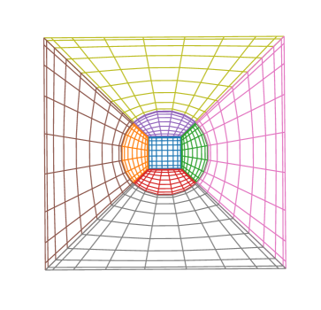
Figure 1: The plot shows some domains and their coordinate lines in the $xy$-plane. Plotted are the domains inside and around neutron star 1. The star is roughly spherical and covered by a central cube and six cubed sphere wedges, four of which are shown because they intersect the $xy$-plane. The space around the star is covered by six more domains to form a larger cube.

In Fig. 1 we show the coordinate lines in $z=0$ plane. The star is covered by a central cube surrounded by several cubed sphere wedges. The space around the star is covered by several more domains. All domains together cover a larger cube containing the star and its surroundings. The coordinate transformation for the green wedge covering the star interior to the right of the central cube is given by

$$x = x_{C*}+(a_{1}-a_{0})\lambda+a_{0},$$

$$y = y_{C*}+\left[(a_{1}-a_{0})\lambda+a_{0}\right]A,$$

$$z = z_{C*}+\left[(a_{1}-a_{0})\lambda+a_{0}\right]B,$$ (27)

where $\lambda\in[0,1]$, $A,B\in[-1,1]$ and

$$a_{1}=\frac{\sigma_{1}(A,B)}{\sqrt{1+A^{2}+B^{2}}},\ \ \ a_{0}=const.$$ (28)

The function $\sigma_{1}(A,B)$ determines the shape of the star surface. Notice that for $\sigma_{1}(A,B)=R_{*}=const$ we obtain a spherical star surface with radius $R_{*}$. The coordinate lines in Fig. 1 are obtained for $B=0$. The coordinate transformation for the other wedges inside the star can be obtained by exchanging $x$ with $y$ or $z$ and by possible sign changes of $a_{1}$ and $a_{0}$. For example the red wedge covering the star interior below the central cube is given by

$$y = y_{C*}+(a_{1}-a_{0})\lambda+a_{0},$$

$$x = x_{C*}+\left[(a_{1}-a_{0})\lambda+a_{0}\right]A,$$

$$z = z_{C*}+\left[(a_{1}-a_{0})\lambda+a_{0}\right]B,$$ (29)

where now

$$a_{1}=-\frac{\sigma_{1}(A,B)}{\sqrt{1+A^{2}+B^{2}}},\ \ \ a_{0}=-const.$$ (30)

The inverted wedges just outside the stars are obtained by reversing the roles of $a_{1}$ and $a_{0}$. For the domain just below the red wedge we would have

$$a_{0}=-\frac{\sigma_{1}(A,B)}{\sqrt{1+A^{2}+B^{2}}},\ \ \ a_{1}=-const,$$ (31)

while still using Eqs. (III.1).

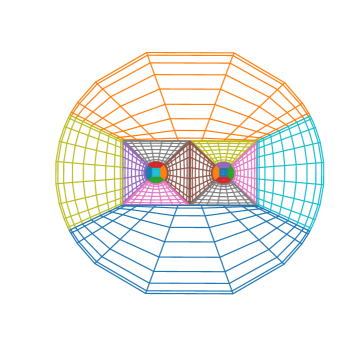
Figure 2: The plot shows the domains in and around both stars augmented by several more domains. The result is a large sphere that covers both stars and their surroundings.

Fig. 2 shows how two such larger cubes as in Fig. 1 can be put next to each other, and in turn be surrounded by more wedges so as to cover a large sphere. This sphere can in turn be surrounded by shells that can be obtained by choosing

$$a_{0}=\frac{\sigma_{in}}{\sqrt{1+A^{2}+B^{2}}},\ \ \ a_{1}=\frac{\sigma_{out}}{\sqrt{1+A^{2}+B^{2}}},$$ (32)

where $\sigma_{in}$ and $\sigma_{out}$ denote the inner and outer radius of the shell. Since we have to impose the boundary conditions of Eqs. (23) at infinity one should choose $\sigma_{out}$ to be very large. For a given number of grid points in $\lambda$, this, however, will result in poor resolution in the radial direction, which could adversely affect the accuracy of our method. For this reason we introduce yet another coordinate transformation. If we define $r:=\sqrt{x^{2}+y^{2}+z^{2}}$ and $L:=\sigma_{out}-\sigma_{in}$, then Eqs. (III.1) and (32) result in

$$r=L\lambda+\sigma_{in}.$$ (33)

So if we want a domain that extends to a large radius it is advantageous to replace the $\lambda$ coordinate with

$$\rho=\frac{\sigma_{out}}{L}\left(1-\frac{\sigma_{in}}{r}\right)=\frac{\sigma_{out}}{L}\left(1-\frac{\sigma_{in}}{L\lambda+\sigma_{in}}\right).$$ (34)

Then a quantity $\Psi$ that behaves as $\Psi\sim b_{1}+b_{2}/r$ for large $r$, becomes $\Psi\sim c_{1}+c_{2}\rho$, when expressed in terms of $\rho$ (here $b_{1}$, $b_{2}$, $c_{1}$, $c_{2}$ are constants). Thus, if within our spectral method we expand $\Psi(\rho)$ in terms of Chebychev polynomials only the first few coefficients will be non-negligible, which leads to a very good approximation when we keep only a finite number of terms. This would not be the case if we used $\lambda$ as our coordinate since then $\Psi\sim d_{1}+d_{2}/\lambda$, which is not a polynomial in $\lambda$.

III.2 Non-linear equations we have to solve

In order to construct initial data we have to solve the elliptic equations (13), (14), (15), and (16). This is done using SGRID’s pseudospectral method as in Tichy (2006, 2009a, 2009b) where we use Chebychev expansions and introduce grid points at the Chebychev extrema. Once the number of grid points is chosen all derivatives are approximated by certain linear combinations of the field values at the grid points. Such a pseudospectral method is similar in spirit to finite differences but it uses all grid points in one direction to approximate a derivative in this direction and is, thus, much more accurate for smooth fields. Once all derivatives have been discretized in this way, we end up with a set of non-linear equations for all fields at all grid points. This system of equations has the form

$$F_{m}(U)=0,$$ (35)

where the solution vector $U$ is comprised of all the fields at all grid points, i.e.,

$$U=(\psi_{0},\psi_{1},...,B^{i}_{0},B^{i}_{1},...,(\alpha\Psi)_{0},(\alpha\Psi)_{1},...,\phi_{0},\phi_{1},...),$$ (36)

where the subscripts label the grid points. Note, however, that we also have to solve the algebraic equation (17), which is done in an iterative manner. We update $h$ and thus the matter distribution after the elliptic equations have been solved, and then the elliptic equations are solved again until we reach a certain tolerance. Because we have to iterate anyway, we do not solve the full system of equations (36), but rather solve the equations for $\psi$, $B^{i}$, $\alpha\Psi$, and $\phi$ individually one after the other within the overall iteration. Then the non-linear system of equations we solve at once is

$$f_{m}(u)=0,$$ (37)

where $u$ is now one of the six fields $\psi$, $B^{i}$, $\alpha\Psi$ or $\phi$. To find the solutions we use a Newton-Raphson scheme where $u$ is updated according to $u_{new}=u_{old}+x$ until a desired tolerance has been reached. As in any Newton scheme the correction $x$ is obtained by solving the linearized equations

$$\frac{\partial f_{m}(u)}{\partial u^{n}}x^{n}=-f_{m}(u).$$ (38)

The challenging part of the method is then to find an efficient way to solve this system of coupled linear equations. In the past, Refs. Tichy (2006, 2009a, 2009b); Dietrich et al. (2015), when using only 6 domains we were able to use a direct solver for the sparse matrix $\frac{\partial f_{m}(u)}{\partial u^{n}}$. However now that we are using 38 domains this is now longer efficient. We thus use an iterative generalized minimal residual (GMRES) solver. This solver needs a good preconditioner, otherwise it will take too many iterations to find a solution to the linearized equations. A preconditioner is essentially an approximate inverse of the matrix $\frac{\partial f_{m}(u)}{\partial u^{n}}$ that can be computed efficiently. Here we use a block Jacobi method Reifenberger (2013), i.e., we keep only certain blocks of the matrix $\frac{\partial f_{m}(u)}{\partial u^{n}}$ along the diagonal. Such a block diagonal matrix $P$ is much easier to invert and thus $P^{-1}$ can be used as a preconditioner. We obtain these blocks by first dropping all entries in $\frac{\partial f_{m}(u)}{\partial u^{n}}$ that couple different computational domains. This results in 38 smaller blocks, each of which can be inverted more easily than the full matrix $\frac{\partial f_{m}(u)}{\partial u^{n}}$. To further speed up the computation of the preconditioner, we subdivide each box along both the $A$ and $B$ coordinate directions so that we end up with $2\times 2\times 38=152$ even smaller blocks along the diagonal of $P$, which can now be readily inverted by a direct solver for sparse matrices Davis and Duff (1997, 1999); Davis (2004a, b, ). This block diagonal inverse $P^{-1}$ is used as our preconditioner for the GMRES method, which allows us to solve the linear system in Eq. (38), so that we can take a Newton step.

Since we solve Eqs. (13), (14), (15), and (16) on 38 computational domains we need interdomain boundary conditions that connect them. In principle, these interdomain boundary conditions are very simple. One imposes that each field and its normal derivative are continuous across every interdomain boundary. These conditions are imposed by replacing the elliptic equation at each boundary point by either

$$u=u_{\mbox{adj}}$$ (39)

or

$$n^{i}\partial_{i}u=n^{i}\partial_{i}u_{\mbox{adj}},$$ (40)

where $u_{\mbox{adj}}$ is the field value in the adjacent domain, and $n^{i}$ is the vector normal to the boundary. Since both conditions have to be satisfied, one of them is imposed on the boundary points on one side of the boundary and the other is imposed on the other side in the adjacent domain. For the full system in Eq. (37) it does not matter which condition is used on which side. However, the preconditioner which contains blocks that come from only one domain is sensitive to this issue. It turns out that if one imposes condition (40) on all sides of a domain, the block corresponding to this domain has a determinant of zero and thus cannot be inverted. In SGRID this problem is avoided by making sure that condition (39) is imposed on at least one boundary of each domain. SGRID now has a facility that automatically finds interdomain boundaries and imposes consistent conditions on them.

III.3 Modification to conformal factor equation

The conformal factor $\psi$ has to satisfy Eq. (13). Unfortunately this equation is not guaranteed to have unique solutions. When this happens the linear solver fails and one cannot find initial data. We have observed that this does indeed happen when we try to construct initial data for very compact stars. The problem can easily be seen for zero shift ($B^{i}=0$) where Eq. (13) takes the simple form

$$\bar{D}^{2}\psi=-2\pi\rho\psi^{5}.$$ (41)

If we linearize it we obtain

$$\bar{D}^{2}\delta\psi=-10\pi\rho\psi^{4}\delta\psi,$$ (42)

where $\delta\psi$ is the linearized conformal factor. Linear elliptic equations of this type are well known, and one can prove uniqueness only if the coefficient in front of $\delta\psi$ on the right hand side is positive (see e.g. Gourgoulhon (2007)). However, since both $\rho$ and $\psi$ are positive this coefficient is negative. One can fix this problem by introducing a rescaled density

$$\bar{\rho}=\psi^{8}\rho$$ (43)

so that Eq. (13) becomes

$$\bar{D}^{2}\psi=-2\pi\bar{\rho}\psi^{-3}-\frac{\psi^{5}}{32\alpha^{2}}(\bar{L}B)^{ij}(\bar{L}B)_{ij}.$$ (44)

If we keep $\bar{\rho}$ constant while we solve this equation, its linearized version is

$$\bar{D}^{2}\delta\psi=+6\pi\bar{\rho}\psi^{-4}\delta\psi-\frac{5\psi^{4}}{32\alpha^{2}}(\bar{L}B)^{ij}(\bar{L}B)_{ij}\delta\psi,$$ (45)

which now is guaranteed to have unique solutions for $B^{i}=0$. The downside of this approach is that instead of solving the equation once, one has to solve it iteratively. After each elliptic solve for $\psi$ one has to recompute $\bar{\rho}$ using Eq. (43), and then solve again until the changes in $\psi$ fall below a specified tolerance. However, as described below we have to solve our system of equations using an iterative approach anyway. We thus rescale $\rho$ according to Eq. (43) and only update $\bar{\rho}$ at the start of each overall iteration.

III.4 Modification to velocity potential equation near the star surface

Notice that the elliptic equation (16) for the velocity potential $\phi$ reduces to a first order equation at the star surface where $\rho_{0}\to 0$. In fact it reduces to Eq. (24) which we use as boundary condition on the star surface. Nevertheless, in the star interior we solve Eq. (16). For challenging cases with high spins or high masses we find numerical problems close to the star surface arising from this equation. In these cases the first derivatives of $\phi$ can develop visible kinks just inside the star surface. These kinks tend to destabilize the overall iteration so that we cannot readily compute initial data. We have found that we can smooth out these kinks by replacing Eq. (16) with

$$\frac{c(\rho_{0})\alpha}{h}\psi^{-4}\partial^{2}\phi+2\frac{\rho_{0}\alpha}{h}\psi^{-5}(\partial_{i}\psi)(\partial_{i}\phi)$$

$$+\left(D_{i}\frac{\rho_{0}\alpha}{h}\right)\left(D^{i}\phi\right)+D_{i}\left[\frac{\rho_{0}\alpha}{h}w^{i}-\rho_{0}\alpha u^{0}(\beta^{i}+\xi^{i})\right] = 0.$$

In the first term we have added the function

$$c(\rho_{0})=\rho_{0}+\epsilon\rho_{0c}\left(\frac{\rho_{0c}-\rho_{0}}{\rho_{0c}}\right)^{4},$$ (47)

which depends on a small number $\epsilon$ and on $\rho_{0c}$ which we choose equal to $\rho_{0}$ at the star center. For $\epsilon=0$ we recover Eq. (16). But for positive $\epsilon$ the principal part of Eq. (III.4) now never vanishes. With this modification we are able to find solutions also in more challenging cases. Notice that $c(\rho_{0})=\rho_{0}$ at the star center and that $c(\rho_{0})$ differs from $\rho_{0}$ mostly near the star surface. Since at the star surface we impose the boundary condition (24) that is derived from the unmodified Eq. (16), the modifications to $\phi$ are small.

The neutron star surfaces always coincide with domain boundaries so that it is straightforward to impose the boundary condition (24) for $\phi$ at each star surface. Notice, however, that Eq. (16) and its boundary condition in Eq. (24) do not uniquely specify a solution $\phi$. If $\phi$ solves both Eqs. (16) and (24) $\phi+\mbox{const}$ will be a solution as well. In order to obtain a unique solution we demand that $\phi$ is zero at the star center, i.e. $\phi(x^{i}_{C*})=0$. We impose this condition by adding the term $\phi(x^{i}_{C*})$ to Eq. (III.4) on all grid points in the cubic domain covering the star center.

III.5 Iteration scheme

The elliptic equations (44), (14) and (15) need to be solved in all domains, while the matter equations (III.4) and (17) are solved only inside each star. In order to solve the elliptic Eqs. (44), (14), (15), and (III.4) we need a fixed domain decomposition. However, the location of the star surfaces (where $h=1$) is not known a priori, but rather determined by Eq. (17). For this reason we use the following iterative procedure:

1. We first find an initial guess for $h$ within each star, in practice we simply choose Tolman-Oppenheimer-Volkoff solutions (see e.g. Chap. 23 in Misner et al. (1973)) for each. For the irrotational velocity potential we choose $\phi=\Omega(x_{C*}^{1}-x_{CM}^{1})x^{2}$, where $x_{C*}^{1}$ and $x_{CM}^{1}$ are the center of the star and the center of mass. We choose the initial orbital angular velocity according to post-Newtonian theory.

2. If the residual of Eq. (III.4) is larger than 10% of the combined residuals of Eqs. (44), (14), and (15), we solve Eq. (III.4) for $\phi$. We then reset $\phi$ to $\phi=0.2\phi_{ell}+0.8\phi_{old}$, where $\phi_{ell}$ is the just obtained solution of Eq. (III.4) and $\phi_{old}$ is the previous value of $\phi$.

3. Next we solve the 5 coupled elliptic equations (44), (14), and (15) for $\Psi_{ell}=(\psi,B^{i},\alpha)_{ell}$. We then set $\Psi=(\psi,B^{i},\alpha)$ to $\Psi=0.2\Psi_{ell}+0.8\Psi_{old}$.

4. In order to solve Eq. (17) we need to know the values of the constants $C_{\pm}$ in each star as well as $\Omega$ and $x_{CM}^{1}$. We want to keep the star centers $x_{C*{1/2}}^{1}$ fixed at their initial position, so that the stars do not drift around during the iterations. The location of each star center is given by $\partial_{1}h|_{x_{C*{1/2}}^{1}}=0$. Note that this condition depends on $\Omega$ and $x_{CM}^{1}$. One strategy to find $\Omega$ and $x_{CM}^{1}$ is thus to use a root finder to adjust $\Omega$ and $x_{CM}^{1}$ until this condition is satisfied. This method is known as ”force balance”. In some cases we use this force balance method. However, often it is advantageous to fix $\Omega$ by other means, e.g. by using an eccentricity reduction procedure as described in Appendix B. In this case one only needs to find $x_{CM}^{1}$. This can be achieved by adjusting $x_{CM}^{1}$ such that the $y$-component of the ADM linear momentum is zero. Here the $y$-direction denotes the direction perpendicular to both the orbital angular momentum and the line connecting the two star centers.

5. Next, we use Eq. (17) to update $h$ in each star, while at the same time adjusting $C_{\pm}$ such that the rest mass of each star remains constant. The domain boundaries need to be adjusted (by changing the surface functions such as $\sigma_{1}(A,B)$ in Eq. (28)) so that they remain at the star surfaces, which change whenever $h$ is updated.

6. We then evaluate the residuals [i.e. the $L^{2}$-norm of the left hand sides of Eqs. (44), (14), (15), and (III.4)]. If the combined residual is below a prescribed tolerance we are done and exit the iteration at this point.

7. In order to ensure that the star centers always remain at their original position we use a root finder to find the locations where $\partial_{i}h=0$. We then translate $h$ (and all other matter variables such as $\rho_{0}$ and $P$) by the amount necessary to bring them back to the original $x_{C*{1/2}}^{1}$.

8. Finally we go back to step 2.

IV Mass, center, momentum, and spin of individual stars

In General Relativity no unambiguous definitions for the mass and spin of an individual star in a binary system exist. Here we introduce easy to compute estimates for such local quantities; see also e.g. Campanelli et al. (2007); Tacik et al. (2015); Dietrich et al. (2017a).

A star mass estimate can be obtained from

$$M:=-\frac{1}{2\pi}\int_{*}f^{kl}\partial_{k}\partial_{l}\psi\sqrt{f}d^{3}x.$$ (48)

This equation has the same form as the ADM mass for conformally flat metrics, however, the integration runs only over the star. Here $f_{ij}=\delta_{ij}$ is the flat conformal metric. We find that this quantity is much closer to the mass of an individual star with the same baryonic mass than an analog definition using the physical metric $\gamma_{ij}=\psi^{4}f_{ij}$ in place of $f_{ij}$. Also, if one considers the special case of the Schwarzschild metric in conformally flat isotropic coordinates, the above definition yields the correct mass, while a definition using the physical metric $\gamma_{ij}$ would give a mass that is too large.

Since the above integral seems to capture the mass aspect of a star, we introduce an analogous integral to define the center of the star

$$R_{c}^{i}:=-\frac{1}{2\pi}\int_{*}\frac{x^{i}-x_{CM}^{i}}{M}f^{kl}\partial_{k}\partial_{l}\psi\sqrt{f}d^{3}x.$$ (49)

This is essentially the same integral, except now weighted with the coordinate $x^{i}$ divided by the mass $M$.

In order to obtain a momentum estimate we start with

$$P(k)=\frac{1}{8\pi}\oint_{*}K_{ij}k^{i}n^{j}\sqrt{q}d^{2}y,$$ (50)

which is again inspired by the definitions for the ADM linear and angular momenta (see e.g Gourgoulhon (2007)). However the integration here runs only over the surface of the star. Here, $n^{i}$ is the normal vector of the star surface and $q$ is the determinant of the metric induced on the surface by the physical metric and is given by

$$q_{ij}=\gamma_{ij}-n_{i}n_{j},\ \ n_{i}=\gamma_{ij}n^{j},\ \ n_{i}n^{i}=1.$$ (51)

The vector $k^{i}$ is a symmetry vector that could be a translational or rotational Killing vector resulting in linear or angular momentum. However since no exact Killing vectors will exist in the case of binaries, and also to keep things simple, we will construct $k^{i}$ from the coordinate unit vectors $(1,0,0)$, $(0,1,0)$, $(0,0,1)$ for the case of linear momentum, and from the coordinate rotation vectors $(1,0,0)\times\vec{r}$, $(0,1,0)\times\vec{r}$, $(0,0,1)\times\vec{r}$, where $\vec{r}=(x,y,z)$. For linear momentum and angular momentum about $\vec{x}_{CM}$ we thus obtain

$$P^{i}:=\frac{1}{8\pi}\oint_{*}K_{il}n^{l}\sqrt{q}d^{2}y,$$ (52)

and

$$J^{i}:=\frac{1}{8\pi}\oint_{*}K_{kl}n^{l}\epsilon^{ijk}(x^{j}-x_{CM}^{j})\sqrt{q}d^{2}y.$$ (53)

Notice that we would obtain the same results for $P^{i}$ and $J^{i}$ if we had defined them using the conformal $\bar{K}_{ij}=\psi^{2}K_{ij}$ while at the same time defining $q_{ij}$ to be the metric induced by the conformal metric $f_{ij}$. Also note that the usual surface integrals at infinity for ADM linear momentum and angular momentum can be converted into volume integrals. These volume integrals have support only within the stars, so that a natural definition for the star momentum is just this volume integral over the star. Furthermore each such volume integral over the star can be rewritten in terms of a surface integral over the star surface. The expressions for the resulting surface integrals are the same as Eqs. (52) and (53). This means that for a binary the $J^{i}$ for each star will add up to the total ADM angular momentum. These facts should give us a measure of confidence in the definitions (52) and (53), probably more confidence than in the mass definition (48), where such arguments do not apply.

Now that we can compute linear and angular momentum as well as the star center, we can define the star spin in the usual way as

$$S^{i}:=J^{i}-\epsilon^{ijk}R_{c}^{j}P^{k}.$$ (54)

The biggest uncertainty in this expression comes from $R_{c}^{j}$. However, since $R_{c}^{j}$ computed using Eqs. (48) and (49) is a ratio of integrals, errors in the mass definition may at least partially divide out.

V Numerical results: Initial data construction

V.1 Initial data sequences

As a first test of the upgraded SGRID code, we compute for four sets of binary parameters initial data sequences comparing the results of the old and the new SGRID implementation (see also Appendix C). All configurations employ a piecewise-polytropic fit of the SLy EOS Read et al. (2009); Dietrich et al. (2015). The gravitational masses are either $m_{1}=m_{2}=1.375M_{\odot}$ with mass ratio $q=1$, or $m_{1}=1.445M_{\odot},m_{2}=1.156M_{\odot}$ with mass ratio $q=1.25$, combined with the dimensionless spins $\chi=0$ and $\chi=0.05$. Figure 3 shows the ADM angular momenta ($J_{\rm ADM}$, top panel) and ADM masses ($M_{\rm ADM}$, bottom panel) as a functions of orbital velocity $(M\Omega)$ for all four configurations and for the new and old SGRID code (dashed lines). The slight differences for large separations, i.e., small orbital frequencies, might be due to different eccentricities of the individual setups.

In Fig. 4, we plot the binding energy

$$E_{b}=\frac{1}{\nu}\left(\frac{M_{ADM}}{M}-1\right)$$ (55)

versus the reduced orbital angular momentum

$$l=\frac{L}{\nu M^{2}}=\frac{J_{ADM}-S_{1}-S_{2}}{\nu M^{2}}.$$ (56)

Here $\nu=m_{1}m_{2}/M^{2}$ is the symmetric mass ratio, $M$ is the total mass and $S_{1,2}$ are the individual spin magnitudes.

In Fig. 4, the solid lines represent the new SGRID data while the dashed curves represent results obtained with the previous code version. We find that both results are in good agreement with each other, which validates our new implementation.

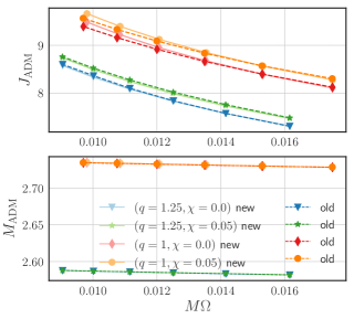
Figure 3: ADM-angular momentum ($J_{ADM}$) and mass ($M_{ADM}$) as a function of the angular orbital velocity $M\Omega$. Solid lines refer to results obtained with the new SGRID code, dashed lines are obtained with the old implementation.

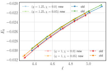
Figure 4: Binding energy $E_{b}$ as function of the reduced orbital angular momentum $\ell$ for different configurations as discussed in the main text. Solid lines show the results for the new, and dashed lines for the old SGRID implementation.

V.2 Testing our spin definition for individual stars

In Tab. 1 we show results of our mass and spin definitions, Eqs.(48) and (54), for the case of a single star and a BNS system with and without spin. We see that the mass definition (48) for an individual star differs from the ADM mass in isolation (which is $m=1.64$) by about 1% in the case of a binary, and is exact only for a single non-spinning star. The spin definition is exact for a single star and the spin estimates for binaries are very likely better than 1% accurate , because of the partial cancellation of errors in $R^{i}_{c}$ discussed in Sec. IV.

$m_{0}=1.7745$ $\rightarrow$ TOV $m=1.64$	$M_{1}$	$S_{1}$	$S_{1}/m^{2}$
one non-spinning star ($\omega=0$)	1.640	0	0
one spinning star ($\omega=0.01525$)	1.646	$+0.8706$	$+0.3237$
two non-spinning stars ($\omega=0$)	1.620	$-0.0007$	$-0.0003$
two spinning stars ($\omega=0.01525$)	1.626	$+0.8652$	$+0.3217$

Table 1: Mass and spin estimates for the case of a polytropic equation of state $P=\kappa\rho_{0}^{1+1/n}$ with $\kappa=123.6$, $n=1$. For a binary with separation of $47.2$ (with $\Omega=0.005096$), the mass definition differs from the ADM mass in isolation by about 1%. The spin definition is exact for a single star, and it is almost the same for a single star and a star in a binary if the spin angular velocity ($\omega=0.01525$) is the same in both cases.

In Fig. 5 we show the spin computed with Eq. (54) versus the spin angular velocity $\omega$ for an equal mass binary with equal spins aligned with the orbital angular momentum.

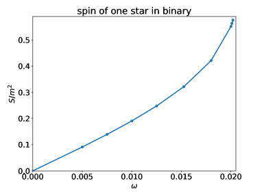
Figure 5: Dimensionless spin of one star in an equal mass binary with $m_{1/2}=1.64$, $r_{12}=47.2$, using a polytropic equation of state with $\kappa=123.6$, $n=1$.

In this case we can reach a spin of $S/m^{2}=0.5763$ at $\omega=0.0202$, which is slightly beyond the mass shedding limit of about $0.5705$ for a single star with this polytropic equation of state Ansorg et al. (2003). If we further increase $\omega$, SGRID fails. This happens because during the iterations the star expands far into the domains that are supposed to be outside of the star such that it is impossible to adjust our domains to be surface fitting. We think that this is not a true failure of the the program and should be expected to happen, since the stars will shed mass at these spin angular velocities.

VI Numerical results: Dynamical Evolutions

VI.1 Evolving millisecond pulsars

resolution	$m_{1,2}^{\rm quasi-loc.}$	$\chi_{1,2}^{\rm quasi-loc.}$	$m_{1,2}^{\rm singl.\ star}$	$\chi_{1,2}^{\rm signl.\ star}$	$M_{\rm ADM}$	$J_{\rm ADM}$
$22\times 22\times 22$	1.346800	0.59466	1.364748	0.57536	2.711566	9.8464958
$26\times 26\times 26$	1.346948	0.59474	1.365494	0.57504	2.711535	9.8494049

Table 2: Mass and dimensionless spin for different resolutions for the binary millisecond configuration, as well as the ADM mass and angular momentum. The NS spin and mass estimates are computed from the quasi-local measures introduced before and from a comparison to single star values estimated from isolated stars with the same EOS, baryonic mass, and rotational velocity as the individual constituents of the binary system.

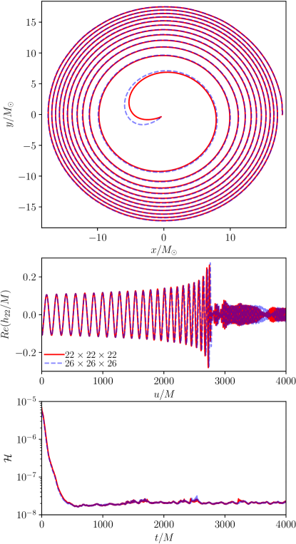
Figure 6: NS tracks of a binary pulsar system as described in Tab. 2 for two different resolutions (top panel). Real part of the dominant (2,2)-mode of the GW signal ($Re(h_{22})$) for both resolutions (middle panel) and Hamiltonian constraint (bottom panel).

As discussed in the introduction, NSs are expected to be spinning and a number of millisecond pulsars have been observed already (although none of them bound in a BNS system). To proof that our upgraded SGRID version is capable of simulating millisecond pulsars, we will present an equal mass, aligned spin configuration in which the individual baryonic masses of the two stars are $m_{1,2}^{b}=1.494607$ and the rotational velocity, Eq. (25), is set to $\omega_{1,2}=0.03$.

We compute initial configurations for this system with two different SGRID resolutions, using $22\times 22\times 22$ and $26\times 26\times 26$ points in all domains. While the lower resolution result for this challenging configuration can be computed in $52.4$ hours, the higher resolution run takes about $93.2$ hours. Both initial data computations were performed on a single Intel Xeon node with 20 cores on FAU’s Koko cluster. Due to the different resolutions, the initial configurations are slightly different, as shown in Tab. 2. We find differences within the estimated masses of about $2\%$ and dimensionless spins of about $3\%$ between the quasi-local mass/spin measure (Sec. IV) and the single star properties of a NS with the same EOS, baryonic mass, and rotational velocity. These differences show that the introduced quasi-local mass measure allows only an approximate extraction of the individual masses for binary configurations. For a high-quality analysis of high-resolution data $2\%$ differences in the individual masses, i.e., absolute differences of the order of $\sim 10^{-3}$, are well above the acceptable uncertainty of an analysis of the energetics of the system for which uncertainties of $\sim 10^{-5}$ are typically required; see e.g. Damour et al. (2012); Bernuzzi et al. (2014); Dietrich and Hinderer (2017). We thus recommend to use the ADM mass of a single star with the same baryonic mass and spin as the best available measure for the mass of an individual star. However, the situation is different for the introduced quasi-local spin measure. The fact that there is a $3\%$ difference between the quasi-local spin of a star in a binary and the spin of a single star with the same EOS, baryonic mass, and rotational velocity, does not mean that the quasi-local spin measure has a $3\%$ error. Rather it is quite likely that we are simply comparing two stars with different spins, because using the same rotational velocity ($\omega=0.03$) does not necessarily lead to the same spin when we compare a star in a binary and a single star.

Despite these small differences, each case describes a binary in which both stars spin close to break-up. As far as we know, this is the highest spinning BNS simulation that includes the merger and postmerger, which has been performed until now. We evolve the system with the BAM code using $96$ points within the finest refinement level. This resolution is not sufficient for a highly accurate GW signal needed for waveform model development, but sufficient to show that the simulation of binary millisecond systems is feasible. The NS tracks (for one star), the emitted GW signal, and the Hamiltonian constraint for the two resolutions are shown in Fig. 6. We find almost circular orbits with a residual eccentricity of $\sim 10^{-3}$, due to the employed eccentricity reduction. The difference between the phases of the GW signals shown in the middle panel of Fig. 6 is about $1$ radian at the moment of merger. It is caused by (i) the different resolutions of the initial data, (ii) the slightly different masses of the configurations (cf. Tab. 2), and (iii) by the fact that eccentricity reduction was only applied to the low SGRID resolution, while simply using the same values for $v_{r}$ and $\Omega$ for the high SGRID resolution. The bottom panel shows the Hamiltonian constraints, where we find only minor differences between the two SGRID resolutions.

VI.2 Evolving highly compact stars

In the past we had implemented the Hamiltonian constraint as in Eq. (13) and found that we were able to find a solution only for low compactness. With the modification given by Eq. (44) and described in Sec. III.3 we can now construct much more compact stars. As an example we have considered an equal mass binary without spin, where each star has a baryonic mass of $m_{0}=2.4$ and obeys the SLy equation of state. This baryonic mass corresponds to a gravitational mass of $m=2.0213$ and a compactness of $\left(\frac{m}{R}\right)_{\infty}=0.284$ for each star at infinite separation. The gravitational mass is thus very close to the maximum $m_{max}=2.0606$ possible with the SLy equation of state. As far as we know, it is also the most compact BNS system evolved so far.

We have evolved this binary with BAM using a piecewise-polytropic fit for the SLy EOS Read et al. (2009); Dietrich et al. (2015) with an added thermal contribution to the pressure following a $\Gamma$-law with $\Gamma=1.75$.

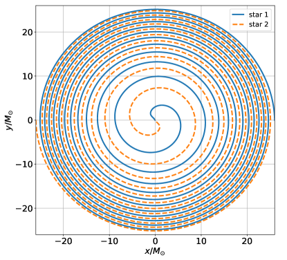
Figure 7: Tracks of the star centers for the equal mass binary with compactness $\left(\frac{m}{R}\right)_{\infty}=0.284$.

In Fig. 7 we show the tracks of the two star centers starting from an inital coordinate separation of $52$ up to merger. The initial orbital angular velocity and radial velocity are $\Omega=0.0048738$ and $v_{r}=-0.00151$. The latter values have been obtained using the eccentricity reduction procedure described in Appendix B.

VI.3 Evolving unequal mass systems

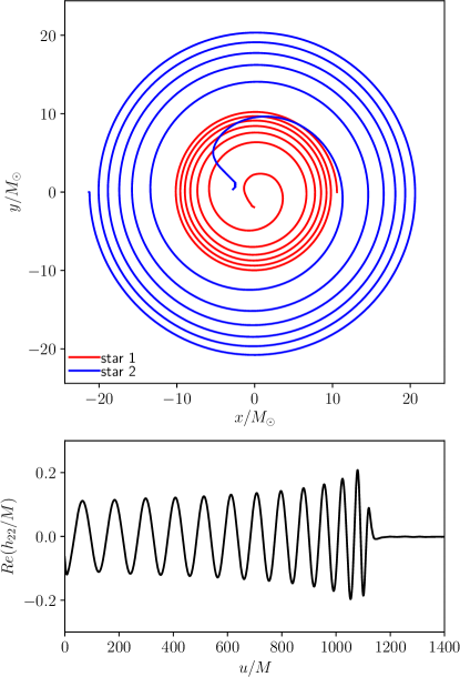
Figure 8: NS tracks of the two stars in our high-mass ratio simulation (top panel) and the real part of the dominant (2,2)-mode of the GW signal (bottom panel).

In order to cover a larger set of configurations for binary neutron stars and to test the capability of the new version of SGRID, we have also constructed the initial data for a high mass ratio system. We chose the configuration to be composed of two non-spinning neutron stars with a piecewise-polytropic fit of the SLy EOS Read et al. (2009); Dietrich et al. (2015) with gravitational mass of $1.99M_{\odot}$ and $0.98M_{\odot}$ which results in a mass ratio of $q=2.03$. This is the highest mass ratio considered for a soft equation of state in numerical relativity for a BNS system. While this mass ratios might even be at the edge of what is theoretically allowed, a study of these kind of systems is essential to develop and improve waveform models, see e.g. Dietrich et al. (2019b).

In Fig. 8 we show the tracks of each neutron star in the binary after three steps of eccentricity reduction. These tracks illustrate the trajectory of center of each neutron star in x-y plane. The center of each neutron star is estimated as the minimum of the lapse inside each star. Near merger, the less massive star is disrupted, which causes the track of the less massive star to end.

In Fig. 8 we show the dominant (2,2)-mode of the GW ($Re(h_{22})$) versus the retarded time. Due to the very large mass of the primary star the system undergoes a prompt collapse to a BH after the moment of merger. The gravitational wave signal thus settles down very quickly after the merger.

VII Summary

In this article, we have presented upgrades made to the SGRID code to improve the capability of constructing initial data for numerical relativity simulations. Among other things our upgrades involve a new grid structure, the use of different coordinates, as well as a reformulation of the equations for the conformal factor and the velocity potential. In order to compare with other methods or models, for example post-Newtonian theory, one would like to know certain physical quantities such as the mass and spin of each star. We have presented simple estimates for the initial mass, spin, momentum, and center of mass of each individual star.

We have tested our new implementation by comparing results against the previous SGRID version and found good agreement between initial data sequences. We also observe lower constraint violations (see Appendix C), and in addition are able to construct more demanding initial data sets with high spins, masses, and mass ratios.

To show that the new code version will be of importance within the field of numerical relativity, we have constructed initial data for a binary system with individual stars close to the breakup, as well as close to the maximum mass allowed by the equation of state, and furthermore a BNS system with a soft equation of state characterized by a high mass ratio of $q=2.03$. All these simulations enter previously unexplored regions of the BNS parameter space. Due to an eccentricity reduction procedure, the presented simulations have typical eccentricities of $\sim 10^{-3}$. This allows their usage for the calibration and validation of gravitational waveform models.

In the future, we plan to use SGRID’s new capabilities to perform new simulations and extend the publicly available CoRe database Dietrich et al. (2018c) with high quality data, previously not accessible within the numerical relativity community.

Appendix A Empirical $\omega$ - $\chi$ relation

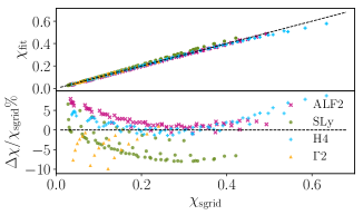
Figure 9: The dimensionless spin according to Eq. 57 as a function of spin computed in the new SGRID for different EOSs (top panel). The fraction residuals are shown in the bottom panel. The black dash curve represents $\chi_{\rm SGRID}=\chi_{\rm fit}$ scenario.

As shown, SGRID can construct initial configurations in which the individual stars are arbitrarily spinning Dietrich et al. (2015); Tichy (2006, 2009a). However, for this, one has to specify the angular velocity of the fluid $\omega$, the baryonic masses, and the EOS as input parameters. The spin itself can not be specified directly. Thus, to minimize computational costs and simplify the computation, we need to find an ansatz for the spin in terms of SGRID’s input parameter. One such phenomenological fit has been given in Appendix C.2 of Ref. Dietrich et al. (2015). However, we found that it might give large errors at high spins, which are now reachable with our new SGRID implementation. Therefore, building upon that, we fit the following data generated for a single star to the SGRID output for $\chi_{\rm SGRID}$. We use 4 EOSs, (SLy, ALF2, H4, and a $\Gamma=2$ polytrope) with baryonic masses $M_{b}/M_{\odot}\in[1.1,1.7]$ in steps of $0.1$ and compactnesses in the range of $\mathcal{C}\in[0.09,0.20]$. We find the following phenomenological fit for the dimensionless spin magnitude $\chi$ of a single NS:

$$\chi_{\rm fit}=a_{1}(1+m_{1}M_{b})(1+c_{1}\mathcal{C}+c_{2}\mathcal{C}^{2}+c_{3}\mathcal{C}^{3}+c_{4}\mathcal{C}^{4})(1+d_{1}\omega)\omega,$$ (57)

where the coefficients $a_{1}=59.329$, $m_{1}=1.9267$, $c_{1}=-17.1537$, $c_{2}=122.8986$, $c_{3}=-401.3542$, $c_{4}=483.0869$, and $d_{1}=10.2497$ are computed by fitting the data, cf. Fig. 9. Specifically, we employ for all combinations of the NS mass and EOS, ten different values of $\omega\in[0.000,0.02]$ in steps of $\Delta\omega=0.002$. The fractional residuals for each configuration is shown in the bottom panel Fig. 9. The new fit gives maximum 10% error for some extreme cases otherwise the error is below 5%.

Appendix B $\Omega$ based eccentricity reduction procedure

In most cases we have used an eccentricity reduction procedure very similar to the one in Tacik et al. (2015), instead of the one described in Dietrich et al. (2015), because in many cases it is advantageous to avoid using the “force balance” relation mentioned in point 4 of Sec. (III.5).

We start with a post-Newtonian estimate for $\Omega$ as well as $v_{r}=0$. We then evolve for about three orbits and fit the observed distance $d(t)$ between the star centers to

$$S(t)=S_{0}+A_{0}t+\frac{A_{1}}{2}t^{2}-\frac{B}{\omega_{f}}\cos(\omega_{f}t+\phi),$$ (58)

where $S_{0}$, $A_{0}$, $A_{1}$, $B$, $\omega_{f}$, and $\phi$ are fit parameters. From the fit parameters we compute the measured eccentricity

$$e=-\frac{B}{\omega_{f}d_{0}}$$ (59)

as well as the changes

$$\delta v_{r}=-B\sin\phi,\ \ \ \delta\Omega=-\frac{B\omega_{f}\cos\phi}{2\Omega d_{0}}$$ (60)

in $v_{r}$ and $\Omega$ needed to lower the eccentricity. We then recompute initial data with the thus changed values for $v_{r}$ and $\Omega$, and evolve and fit again to obtain the next set of changes to $v_{r}$ and $\Omega$. We usually perform 3 or 4 such reduction steps. Notice that we typically use the proper distance as the distance measure $d(t)$ that we fit, and that we set $d_{0}$ equal to the initial coordinate distance. The latter has given slightly better estimates for $\delta v_{r}$ and $\delta\Omega$ than simply setting $d_{0}=S_{0}$.

Appendix C Comparison with the old version of SGRID

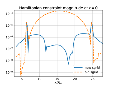
Figure 10: The Hamiltonian constraint across one of the stars at the initial time for both the old (broken line) and new (solid line) version of SGRID. Similar violations occur in both approaches near the star surfaces, but inside the stars the new version shows less violations.

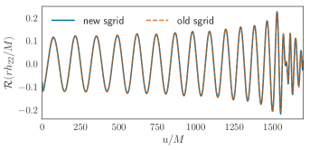
Figure 11: Comparison between the GW signals computed for the same physical configurations computed with the old and new SGRID code. Old SGRID results are shown with an orange dashed line, new SGRID results with a blue, solid curve.

In order to test the new implementation, we have constructed and evolved initial data with the same physical parameters using the two different SGRID versions. We use the same configuration for both initial data, namely a $\Gamma=2$, $\kappa=123.6489$ EOS. The system is an equal mass binary in which the individual stars have a baryonic mass of 1.625 $M_{\odot}$. The initial separation between the stars is $68.8\rm km$.

Figure 10 shows the Hamiltonian constraint across one of the stars at the initial time after interpolating the SGRID data onto BAM’s grid. As we can see the new SGRID version (solid line) produces smaller constraint violations than the old version (broken line), inside the star, while at the star surfaces both lead to approximately the same violations. Outside the stars, the old SGRID version seems slightly superior.

In Fig. 11 we show the dominant (2,2) mode of GW. We evolve both initial data sets with BAM using exactly the same setup for both evolution, namely 6 refinement and 96 points to cover the star. The GWs are extracted at a distance of 900 $M_{\odot}$. Waveforms are aligned for the two cases at early times, i.e., before $u\leq 600M$. We find that both waves agree very well throughout the merger and in the early post-merger part; see Fig. 11.

References

- Abbott et al. (2017a) B. P. Abbott et al. (LIGO Scientific, Virgo), Phys. Rev. Lett. 119, 161101 (2017a), eprint 1710.05832.
- Abbott et al. (2017b) B. P. Abbott et al. (LIGO Scientific, Virgo, Fermi GBM, INTEGRAL, IceCube, AstroSat Cadmium Zinc Telluride Imager Team, IPN, Insight-Hxmt, ANTARES, Swift, AGILE Team, 1M2H Team, Dark Energy Camera GW-EM, DES, DLT40, GRAWITA, Fermi-LAT, ATCA, ASKAP, Las Cumbres Observatory Group, OzGrav, DWF (Deeper Wider Faster Program), AST3, CAASTRO, VINROUGE, MASTER, J-GEM, GROWTH, JAGWAR, CaltechNRAO, TTU-NRAO, NuSTAR, Pan-STARRS, MAXI Team, TZAC Consortium, KU, Nordic Optical Telescope, ePESSTO, GROND, Texas Tech University, SALT Group, TOROS, BOOTES, MWA, CALET, IKI-GW Follow-up, H.E.S.S., LOFAR, LWA, HAWC, Pierre Auger, ALMA, Euro VLBI Team, Pi of Sky, Chandra Team at McGill University, DFN, ATLAS Telescopes, High Time Resolution Universe Survey, RIMAS, RATIR, SKA South Africa/MeerKAT), Astrophys. J. 848, L12 (2017b), eprint 1710.05833.
- Cook (2000) G. B. Cook, Living Rev. Rel. 3, 5 (2000), eprint gr-qc/0007085.
- Tichy (2017) W. Tichy, Rept. Prog. Phys. 80, 026901 (2017), eprint 1610.03805.
- Haas et al. (2016) R. Haas et al., Phys. Rev. D93, 124062 (2016), eprint 1604.00782.
- Favata (2014) M. Favata, Phys. Rev. Lett. 112, 101101 (2014), eprint 1310.8288.
- Agathos et al. (2015) M. Agathos, J. Meidam, W. Del Pozzo, T. G. F. Li, M. Tompitak, J. Veitch, S. Vitale, and C. V. D. Broeck, Phys. Rev. D92, 023012 (2015), eprint 1503.05405.
- Samajdar and Dietrich (2019) A. Samajdar and T. Dietrich (2019), eprint 1905.03118.
- Hessels et al. (2006) J. W. T. Hessels, S. M. Ransom, I. H. Stairs, P. C. C. Freire, V. M. Kaspi, and F. Camilo, Science 311, 1901 (2006), eprint astro-ph/0601337.
- Lynch et al. (2012) R. S. Lynch, P. C. C. Freire, S. M. Ransom, and B. A. Jacoby, Astrophys. J. 745, 109 (2012), eprint 1112.2612.
- Stovall et al. (2018) K. Stovall et al., Astrophys. J. 854, L22 (2018), eprint 1802.01707.
- Cromartie et al. (2019) H. T. Cromartie et al. (2019), eprint 1904.06759.
- Dietrich and Ujevic (2017) T. Dietrich and M. Ujevic, Class. Quant. Grav. 34, 105014 (2017), eprint 1612.03665.
- Bauswein et al. (2013) A. Bauswein, T. W. Baumgarte, and H. T. Janka, Phys. Rev. Lett. 111, 131101 (2013), eprint 1307.5191.
- Köppel et al. (2019) S. Köppel, L. Bovard, and L. Rezzolla, Astrophys. J. 872, L16 (2019), eprint 1901.09977.
- Hinderer et al. (2010) T. Hinderer, B. D. Lackey, R. N. Lang, and J. S. Read, Phys. Rev. D81, 123016 (2010), eprint 0911.3535.
- Dietrich et al. (2017a) T. Dietrich, S. Bernuzzi, M. Ujevic, and W. Tichy, Phys. Rev. D95, 044045 (2017a), eprint 1611.07367.
- Lehner et al. (2016) L. Lehner, S. L. Liebling, C. Palenzuela, O. L. Caballero, E. O’Connor, M. Anderson, and D. Neilsen, Class. Quant. Grav. 33, 184002 (2016), eprint 1603.00501.
- Zappa et al. (2018) F. Zappa, S. Bernuzzi, D. Radice, A. Perego, and T. Dietrich, Phys. Rev. Lett. 120, 111101 (2018), eprint 1712.04267.
- Kiuchi et al. (2019a) K. Kiuchi, K. Kyutoku, M. Shibata, and K. Taniguchi, Astrophys. J. 876, L31 (2019a), eprint 1903.01466.
- Dominik et al. (2012) M. Dominik, K. Belczynski, C. Fryer, D. E. Holz, E. Berti, T. Bulik, I. Mandel, and R. O’Shaughnessy, Astrophys. J. 759, 52 (2012), eprint 1202.4901.
- Dietrich et al. (2015) T. Dietrich, N. Moldenhauer, N. K. Johnson-McDaniel, S. Bernuzzi, C. M. Markakis, B. Brügmann, and W. Tichy, Phys. Rev. D92, 124007 (2015), eprint 1507.07100.
- Martinez et al. (2015) J. G. Martinez, K. Stovall, P. C. C. Freire, J. S. Deneva, F. A. Jenet, M. A. McLaughlin, M. Bagchi, S. D. Bates, and A. Ridolfi, Astrophys. J. 812, 143 (2015), eprint 1509.08805.
- Lazarus et al. (2016) P. Lazarus et al., Astrophys. J. 831, 150 (2016), eprint 1608.08211.
- (25) LORENE: Langage Objet pour la RElativité NumériquE, http://www.lorene.obspm.fr.
- Kyutoku et al. (2014) K. Kyutoku, M. Shibata, and K. Taniguchi, Phys. Rev. D90, 064006 (2014), eprint 1405.6207.
- East et al. (2012) W. E. East, F. M. Ramazanoglu, and F. Pretorius, Phys. Rev. D86, 104053 (2012), eprint 1208.3473.
- Moldenhauer et al. (2014) N. Moldenhauer, C. M. Markakis, N. K. Johnson-McDaniel, W. Tichy, and B. Brügmann, Phys. Rev. D90, 084043 (2014), eprint 1408.4136.
- Dietrich et al. (2019a) T. Dietrich, S. Ossokine, and K. Clough, Class. Quant. Grav. 36, 025002 (2019a), eprint 1807.06959.
- Tsokaros and Uryu (2012) A. Tsokaros and K. Uryu, J. Eng. Math. 82, 1 (2012), eprint 1207.5833.
- Tsokaros et al. (2015) A. Tsokaros, K. Uryu, and L. Rezzolla, Phys. Rev. D91, 104030 (2015), eprint 1502.05674.
- Foucart et al. (2008) F. Foucart, L. E. Kidder, H. P. Pfeiffer, and S. A. Teukolsky, Phys. Rev. D77, 124051 (2008), eprint 0804.3787.
- Tacik et al. (2015) N. Tacik et al., Phys. Rev. D92, 124012 (2015), eprint 1508.06986.
- Tichy (2006) W. Tichy, Phys. Rev. D74, 084005 (2006), eprint gr-qc/0609087.
- Tichy (2009a) W. Tichy, Class. Quant. Grav. 26, 175018 (2009a), eprint 0908.0620.
- Tichy (2009b) W. Tichy, Phys. Rev. D80, 104034 (2009b), eprint 0911.0973.
- Rüter et al. (2018) H. R. Rüter, D. Hilditch, M. Bugner, and B. Brügmann, Phys. Rev. D98, 084044 (2018), eprint 1708.07358.
- Vincent et al. (2019) T. Vincent, H. P. Pfeiffer, and N. L. Fischer (2019), eprint 1907.01572.
- Bernuzzi et al. (2014) S. Bernuzzi, T. Dietrich, W. Tichy, and B. Brügmann, Phys.Rev. D89, 104021 (2014), eprint 1311.4443.
- Dietrich et al. (2018a) T. Dietrich, S. Bernuzzi, B. Brügmann, and W. Tichy, in Proceedings, 26th Euromicro International Conference on Parallel, Distributed and Network-based Processing (PDP 2018): Cambridge, UK, March 21-23, 2018 (2018a), pp. 682–689, eprint 1803.07965.
- Most et al. (2019) E. R. Most, L. J. Papenfort, A. Tsokaros, and L. Rezzolla (2019), eprint 1904.04220.
- Tsokaros et al. (2019) A. Tsokaros, M. Ruiz, V. Paschalidis, S. L. Shapiro, and K. Uryu (2019), eprint 1906.00011.
- East et al. (2019) W. E. East, V. Paschalidis, F. Pretorius, and A. Tsokaros (2019), eprint 1906.05288.
- Dietrich et al. (2018b) T. Dietrich, S. Bernuzzi, B. Brügmann, M. Ujevic, and W. Tichy, Phys. Rev. D97, 064002 (2018b), eprint 1712.02992.
- Foucart et al. (2016) F. Foucart, R. Haas, M. D. Duez, E. O’Connor, C. D. Ott, L. Roberts, L. E. Kidder, J. Lippuner, H. P. Pfeiffer, and M. A. Scheel, Phys. Rev. D93, 044019 (2016), eprint 1510.06398.
- Kiuchi et al. (2017) K. Kiuchi, K. Kawaguchi, K. Kyutoku, Y. Sekiguchi, M. Shibata, and K. Taniguchi, Phys. Rev. D96, 084060 (2017), eprint 1708.08926.
- Dietrich et al. (2017b) T. Dietrich, S. Bernuzzi, and W. Tichy, Phys. Rev. D96, 121501 (2017b), eprint 1706.02969.
- Foucart et al. (2019) F. Foucart et al., Phys. Rev. D99, 044008 (2019), eprint 1812.06988.
- Dietrich et al. (2019b) T. Dietrich, A. Samajdar, S. Khan, N. K. Johnson-McDaniel, R. Dudi, and W. Tichy (2019b), eprint 1905.06011.
- Kiuchi et al. (2019b) K. Kiuchi, K. Kyohei, K. Kyutoku, Y. Sekiguchi, and M. Shibata (2019b), eprint 1907.03790.
- Chaurasia et al. (2018) S. V. Chaurasia, T. Dietrich, N. K. Johnson-McDaniel, M. Ujevic, W. Tichy, and B. Brügmann, Phys. Rev. D98, 104005 (2018), eprint 1807.06857.
- Dietrich et al. (2018c) T. Dietrich, D. Radice, S. Bernuzzi, F. Zappa, A. Perego, B. Brügmann, S. V. Chaurasia, R. Dudi, W. Tichy, and M. Ujevic, Class. Quant. Grav. 35, 24LT01 (2018c), eprint 1806.01625.
- Radice et al. (2018) D. Radice, A. Perego, K. Hotokezaka, S. A. Fromm, S. Bernuzzi, and L. F. Roberts, Astrophys. J. 869, 130 (2018), eprint 1809.11161.
- Dietrich et al. (2017c) T. Dietrich, M. Ujevic, W. Tichy, S. Bernuzzi, and B. Brügmann, Phys. Rev. D95, 024029 (2017c), eprint 1607.06636.
- Abbott et al. (2019a) B. P. Abbott et al. (LIGO Scientific, Virgo), Phys. Rev. X9, 011001 (2019a), eprint 1805.11579.
- Abbott et al. (2018) B. P. Abbott et al. (Virgo, LIGO Scientific), Phys. Rev. Lett. 121, 161101 (2018), eprint 1805.11581.
- Abbott et al. (2019b) B. P. Abbott et al. (LIGO Scientific, Virgo), Phys. Rev. Lett. 123, 011102 (2019b), eprint 1811.00364.
- Tichy (2011) W. Tichy, Phys. Rev. D84, 024041 (2011), eprint 1107.1440.
- Tichy (2012) W. Tichy, Phys.Rev. D86, 064024 (2012), eprint 1209.5336.
- Rüter (2019) H. Rüter, Ph.D. thesis, Friedrich-Schiller-Universität Jena (2019), URL https://www.db-thueringen.de/receive/dbt_mods_00039088.
- Arnowitt et al. (1962) R. Arnowitt, S. Deser, and C. W. Misner, in Gravitation: An Introduction to Current Research, edited by L. Witten (John Wiley, New York, 1962), pp. 227–265, arXiv:gr-qc/0405109, eprint gr-qc/0405109.
- Read et al. (2009) J. S. Read, B. D. Lackey, B. J. Owen, and J. L. Friedman, Phys.Rev. D79, 124032 (2009), eprint 0812.2163.
- Ansorg (2007) M. Ansorg, Class. Quant. Grav. 24, S1 (2007), eprint gr-qc/0612081.
- Reifenberger (2013) G. Reifenberger, Ph.D. thesis, Florida Atlantic University (2013).
- Davis and Duff (1997) T. A. Davis and I. S. Duff, SIAM J. Matrix Anal. Applic. 18, 140 (1997).
- Davis and Duff (1999) T. A. Davis and I. S. Duff, ACM Trans. Math. Softw. 25, 1 (1999), ISSN 0098-3500.
- Davis (2004a) T. A. Davis, ACM Trans. Math. Softw. 30, 196 (2004a), ISSN 0098-3500.
- Davis (2004b) T. A. Davis, ACM Trans. Math. Softw. 30, 165 (2004b), ISSN 0098-3500.
-
(69)
T. A. Davis,
UMFPACK a sparse linear systems solver using the Unsymmetric
MultiFrontal method:
http://www.cise.ufl.edu/research/sparse/umfpack/. - Gourgoulhon (2007) E. Gourgoulhon (2007), eprint gr-qc/0703035.
- Misner et al. (1973) C. W. Misner, K. S. Thorne, and J. A. Wheeler, Gravitation (W. H. Freeman, San Francisco, 1973).
- Campanelli et al. (2007) M. Campanelli, C. O. Lousto, Y. Zlochower, B. Krishnan, and D. Merritt, Phys. Rev. D75, 064030 (2007), eprint gr-qc/0612076.
- Ansorg et al. (2003) M. Ansorg, A. Kleinwächter, and R. Meinel, Astron. Astrophys. 405, 711 (2003), eprint astro-ph/0301173.
- Damour et al. (2012) T. Damour, A. Nagar, D. Pollney, and C. Reisswig, Phys. Rev. Lett. 108, 131101 (2012), eprint 1110.2938.
- Dietrich and Hinderer (2017) T. Dietrich and T. Hinderer, Phys. Rev. D95, 124006 (2017), eprint 1702.02053.
- Marronetti and Shapiro (2003) P. Marronetti and S. L. Shapiro, Phys. Rev. D68, 104024 (2003), eprint gr-qc/0306075.