Accretion-induced prompt black hole formation in asymmetric neutron star mergers, dynamical ejecta and kilonova signals

Abstract

We present new numerical relativity results of neutron star mergers with chirp mass $1.188M_{\odot}$ and mass ratios $q=1.67$ and $q=1.8$ using finite-temperature equations of state (EOS), approximate neutrino transport and a subgrid model for magnetohydrodynamics-induced turbulent viscosity. The EOS are compatible with nuclear and astrophysical constraints and include a new microphysical model derived from ab-initio calculations based on the Brueckner-Hartree-Fock approach. We report for the first time evidence for accretion-induced prompt collapse in high-mass-ratio mergers, in which the tidal disruption of the companion and its accretion onto the primary star determine prompt black hole formation. As a result of the tidal disruption, an accretion disc of neutron-rich and cold matter forms with baryon masses ${\sim}0.15M_{\odot}$, and it is significantly heavier than the remnant discs in equal-masses prompt collapse mergers. Massive dynamical ejecta of order ${\sim}0.01M_{\odot}$ also originate from the tidal disruption. They are neutron rich and expand from the orbital plane with a crescent-like geometry. Consequently, bright, red and temporally extended kilonova emission is predicted from these mergers. Our results show that prompt black hole mergers can power bright electromagnetic counterparts for high-mass-ratio binaries, and that the binary mass ratio can be in principle constrained from multimessenger observations.

1 Introduction

Binary neutron stars (BNS) mergers are key astrophysical laboratories to explore the fundamental interactions in dynamical and strong gravity. This was clearly demonstrated by the observation of GW170817 Abbott et al. (2017a, 2019a, 2019b) and its related counterparts Abbott et al. (2017b). After GW170817, a second event (GW190425) compatible with a BNS source was reported, indicating a merger rate of 250-2810 Gpc³ per year Abbott et al. (2020). The interpretation of current and future observations rely on quantitative simulations of astrophysically relevant binaries in the framework of numerical relativity (NR). In particular, observational signatures are strongly dependent on the possible NS masses and the still uncertain equation of state (EOS). The latter determine the properties of the final compact object, of the eventual accretion merger remnant and of the observed gravitational and electromagnetic spectra (see Radice et al. 2020 and reference therein for a recent review by some of us.)

The possible NS mass range is ${\sim}0.9-3M_{\odot}$, where the lower bound is inferred from the formation scenario (gravitational collapse) and from current observations e.g. Rawls et al. (2011); Ozel et al. (2012). The upper bound is inferred from a stability argument (Buchdahl limit) and from precise measurements of ${\sim}2M_{\odot}$ NSs in compact binaries containing a millisecond pulsar and a white dwarf  Demorest et al. (2010); Antoniadis et al. (2013); Cromartie et al. (2019). Coalescing cicularized BNS were long expected to have nearly equal masses NS with individual masses around $M_{A}\sim 1.35-1.4M_{\odot}$ and individual spin periods above the millisecond Lattimer (2012); Kiziltan et al. (2013); Swiggum et al. (2015). For example, the source of GW170817 has a total mass of $M\simeq 2.73-2.77M_{\odot}$ and a mass ratio $q\sim 1$ (see below), with the largest uncertainties coming from the spin prior utilized in the analysis Abbott et al. (2019a). This expectation was however challenged by GW190425 that is associated to the heaviest BNS source known to date with $M\simeq 3.2-3.7M_{\odot}$ Abbott et al. (2020). Spins distributions in GW170817 and GW190425 are both compatible with zero Abbott et al. (2019a, 2020).

The mass ratio distribution in BNS (here conventionally defined as the ratio between the most massive primary and the secondary NS, i.e. $q\equiv M_{A}/M_{B}\geq 1$) is very uncertain. BNS population from pulsar observations indicate mass ratios $1\leq q\lesssim 1.4$ Lattimer (2012); Kiziltan et al. (2013); Swiggum et al. (2015). The mass ratio of GW170817 could be as high as $q\sim 1.37$ ($q\sim 1.89$) for low (high) spin priors. Similarly, the mass ratio of GW190425 can be as high as $q\sim 1.25$ ($q\sim 2.5$). Given the expected mass values and the recent observations, it is accepted that BNS mass ratios can reach “extreme” mass ratio $q\lesssim 2$. While these values are not as extreme as those that can be reached in black hole binaries, significant differences for the remnant and radiation signals are expected for BNS with $q\sim 1$ and $q\sim 2$.

Numerical relativity simulations with microphysical EOS performed so far focused on comparable-masses cases and mass ratios $q\lesssim 1.4$ Sekiguchi et al. (2011a, b); Neilsen et al. (2014); Sekiguchi et al. (2015); Palenzuela et al. (2015); Bernuzzi et al. (2016); Sekiguchi et al. (2016); Radice et al. (2016); Lehner et al. (2016); Radice et al. (2017); Radice et al. (2018b, a); Radice et al. (2018c, d). The highest mass ratios of $q=1.5$ and $q=2$ have been simulated with a very stiff piecewise polytropic EOS Dietrich et al. (2015); Dietrich et al. (2017), that is currently disfavored by the GW170817 observation. Mergers of BNS with total mass $M\sim 2.7-2.8M_{\odot}$ and moderate mass ratios up to $q\lesssim 1.4$ with a EOS supporting ${\sim}2M_{\odot}$, are likely to produce remnants that are at least temporarily stable against gravitational collapse to black hole (BH), as opposed to remnants that collapse immediately to BH (prompt BH formation). However, the conditions for prompt BH formation at high-$q$ have not been studied in detail to date. For a given total mass, moderate mass ratios can extend the remnant lifetime with respect to equal mass BNS because of the less violent fusion of the NS cores and a partial tidal disruption that distribute angular momentum at larger radii in the remnant Bauswein et al. (2013a). However, large mass asymmetries $q\gtrsim 1.6$ can favor BH formation due to the larger mass of the primary NS.

Tidal disruption in asymmetric BNS can significantly affect the properties of the dynamical ejecta, favouring a redder kilonova peaking at late times (see e.g. Rosswog et al. 2018; Wollaeger et al. 2018). Moderate mass ratios up to $q\sim 1.3-1.4$ are found to produce more massive discs than $q=1$ BNS Shibata et al. (2003); Shibata & Taniguchi (2006); Kiuchi et al. (2009); Rezzolla et al. (2010); Dietrich et al. (2017). But black hole formation can significantly alter the remnant disc properties, both in terms of compactness and composition Perego et al. (2019). In turn, this can impact the secular (viscous) ejecta component and the kilonova, with bright emissions generally favoured by the presence of a long-lived NS remnant, e.g. Radice et al. (2018d); Nedora et al. (2019). Moreover, assuming the Blandford-Znajek mechanism to be the mechanism launching the relativistic jet that produces a gamma-ray burst, a more massive disc is also expected to power a more energetic jet through a more intense accretion process Shapiro (2017). Many of these aspects are currently not well quantified and they require NR simulations of high mass ratio BNS with microphysics.

In this work, we perform 32 new NR simulations with microphysical EOS, fixed chirp mass $\mathcal{M}_{c}=1.188M_{\odot}$ and mass ratios up $q=1.8$ for four microphysical EOS, including a new microscopic EOS BLh (Sec. 2). The simulations show that for sufficiently high value of the mass ratio (and in a EOS dependent way) the remnant promptly collapses to BH as consequence of the accretion of the companion on the massive primary NS (Sec. 4.) These prompt collapse dynamics is not well described by current NR fitting formulas. By analysing the gravitational waveforms, we further verify current quasiuniversal NR relations for the merger and postmerger gravitational waveforms in the high-$q$ limit (Sec. 5.) We find an overall agreement of the merger relations and characteristic postmerger GW frequencies. But the accurate modeling of postmerger waveforms with high-$q$, will require more simulations and improved methods than those currently employed. We discuss in detail the differences in the dynamical ejecta between the $q=1$ and the high-$q$ mergers in terms of overall ejecta masses, morphology and composition (Sec.6.) High mass ratio and large chirp mass leading to prompt BH formation maximize the dynamical tidal ejecta mass, which is expelled with a peculiar geometry. The $r$-process nucleosynthesis in these neutron-rich ejecta result in bright (more luminous than the $q=1$ case), redder, and temporally extended kilonovae (Sec. 7.)

We employ SI units in most of the paper except for masses, reported in solar masses ($M_{\odot}$), lengths in km, and densities reported in $\mathrm{g~{}cm^{-3}}$. Nuclear density is indicated as $\rho_{0}\approx 2.3\times 10^{14}$ $\mathrm{g~{}cm^{-3}}$. If units are not reported, we then use geometric units $c=G=1$ in context where those are more appropriate (e.g. Sec. 5 and appendices).

2 Equations of state

In this work we consider four finite-temperature, composition dependent EOS: the LS220 EOS Lattimer & Swesty (1991), the SFHo EOS Steiner et al. (2013), the SLy4-SOR EOS Schneider et al. (2017); and the BLh EOS Bombaci & Logoteta (2018). All these EOS include neutrons ($n$), protons ($p$), nuclei, electron, positrons, and photons as relevant thermodynamics degrees of freedom. Cold, neutrino-less $\beta$-equilibrated matter described by these microphysical EOS predicts NS maximum masses and radii within the range allowed by current astrophysical constraints, including the recent GW constraint on tidal deformability Abbott et al. (2017a, 2019a); De et al. (2018); Abbott et al. (2018) (see below). All four models have symmetry energies at saturation density within experimental bounds. However, LS220 has a significantly steeper density dependence of its symmetry energy than the other models, see e.g. Lattimer & Lim (2013); Danielewicz & Lee (2014), and it could possibly underestimate the symmetry energy below saturation density.

The LS220 EOS is based on a non-relativistic Skyrme interaction with the modulus of the nuclear bulk incompressibility set to 220 MeV. Non-homogeneous nuclear matter is modelled by a compressible liquid-drop model including surface effects, and considers an ideal, classical gas formed by $\alpha$ particles and heavy nuclei. The latter are treated within the single nucleus approximation (SNA). The transition between homogeneous and non-homogeneous matter is performed through a Gibbs construction.

The SFHo EOS combines a relativistic mean field approach for the homogeneous nuclear matter to an ideal, classical gas treatment of a statistical ensemble of several thousands of nuclei in Nuclear Statistical Equilibrium (NSE) for the inhomogeneous nuclear matter. The transition between the two phases is achieved by an excluded volume mechanism.

The SLy4 Skyrme parametrization was introduced in Douchin & Haensel (2001) for cold nuclear and NS matter. In this work we employ its extension to finite temperature presented in Schneider et al. (2017) using an improved version of the LS220 model that includes non-local isospin asymmetric terms and a better treatment of nuclear surface properties, and treats the size of heavy nuclei more consistently. The transition between uniform and non-uniform phase is achieved by a first order transition, i.e. choosing the phase with lower free energy.

A main novelty of this work is the use of the BLh EOS, a new finite temperature EOS derived in the framework of non-relativistic Brueckner-Hartree-Fock (BHF) approach (Logoteta et al, in preparation). The corresponding cold, $\beta$-equilibrated EOS was first presented in Bombaci & Logoteta (2018) and applied to BNS mergers in Endrizzi et al. (2018). For the homogeneous nuclear phase, this EOS employs a purely microphysical approach based on a specific nuclear interaction. Consistently with Bombaci & Logoteta (2018), the interactions between nucleons is described through a potential derived perturbatively in Chiral-Effective-Field theory Machleidt & Entem (2011). Specifically, the local potential reported in Piarulli et al. (2016) and calculated up to next to-next to-next to-leading order (N3LO) was used as two-body interaction. This potential takes into account the possible excitation of a $\Delta$-resonance in the intermediate states of the nucleon-nucleon interaction. The above potential was then supplemented by a three-nucleon force calculated up to N2LO and including again the contributions from the $\Delta$-excitation. The parameters of the three-nucleon force were determined to reproduce the properties of symmetric nuclear matter at saturation density Logoteta et al. (2016). For the non-homogeneous nuclear phase there is no straightforward extension of these microphysical methods to sub-saturation densities. Thus, the low density part ($n\leq 0.05~{}{\rm fm^{-3}}$) of the SFHo EOS has been smoothly connected to the high density BLh EOS. This necessary extension has been tested with different finite-temperature, composition-dependented tabulated EOS Hempel & Schaffner-Bielich (2010). They all use 1) relativistic mean field approaches for the homogeneous phase, 2) an ideal, classical gas of a statistical ensemble of several thousands of nuclei in NSE for the non-homogeneous nuclear phase; 3) an excluded volume mechanism to model the transition. No appreciable differences were found in all relevant quantities at subnuclear densities between different high density treatments.

The LS220 and SLy4-SRO EOS are based on Skyrme effective nuclear interactions. In these models thermal effects are introduced starting from a zero temperature internal energy functional that contains an explicit nuclear density dependence. The interaction part of this functional is split into a quadratic term in the nuclear density (playing the role of a two-body nucleon-nucleon interaction) plus a term proportional to some power of the nuclear density. The latter term mimics the effect of many-body nuclear forces. The temperature dependence of the effective nuclear interaction is encoded in the effective mass dependence of the kinetic energy as well as in the single particle potentials. The latter are calculated by the variation of the internal energy with respect to the neutron and proton densities. Assuming indeed a constant entropy, smaller effective masses translate into larger kinetic energies and thus higher matter temperatures. The LS220 EOS assumes that the effective nucleon mass is the bare nucleon mass at all densities while for the SLy4-SRO we have $m_{N}^{*}/m_{N}=0.695$ at saturation density, being $m_{N}^{*}$ and $m_{N}$ the effective and the bare nucleon masses respectively.

In the relativistic Lagrangian underlaying the SHFo EOS, nuclear interactions are described by $\sigma$-, $\omega$- and $\rho$-meson exchanges. The resulting Euler-Lagrange equations are then solved in mean field approximation. In this approach thermal effects are included by introducing Fermi-Dirac distributions at finite temperatures for the various nuclear species. Mesons and nucleon fields, and consequently all thermodynamical quantities, acquire automatically a temperature dependence through the self consistent solution of the mean field equations.

Differently from the other models considered in the present work, thermal effects enter in a quite different way in the BLh EOS. The calculation of the Free energy in the BHF approach Bombaci et al. (1993) requires first the determination of an effective in-medium nuclear interaction, starting from the bare nuclear potential. This effective interaction ($G$-matrix) is obtained by solving the Bethe-Goldstone integral equation which describe the nucleon-nucleon scattering in the nuclear medium and properly takes into account the Pauli principle. Finally, the nucleon single particle potentials $U_{i}(k,T)$ ($i=n,\ p$) is obtained through the integration of the on-shell $G$-matrix. $U_{i}(k,T)$ is a sort of mean field felt by a nucleon of momentum $k$ due to the presence of the surrounding nucleons. The determination of $U_{i}(k,T)$ allows for the calculation of the Free energy from which all the other thermodynamical quantities can be derived. The procedure described above is complicated by the non-linear and non-local dependence of $U_{i}(k,T)$ in Bethe-Goldstone equation. We finally note that this scheme provides many-body correlations which are beyond the mean field approximation. Such correlations are not present in the other EOS models considered in the present paper.

2.1 EOS Constraints and NS equilibrium models

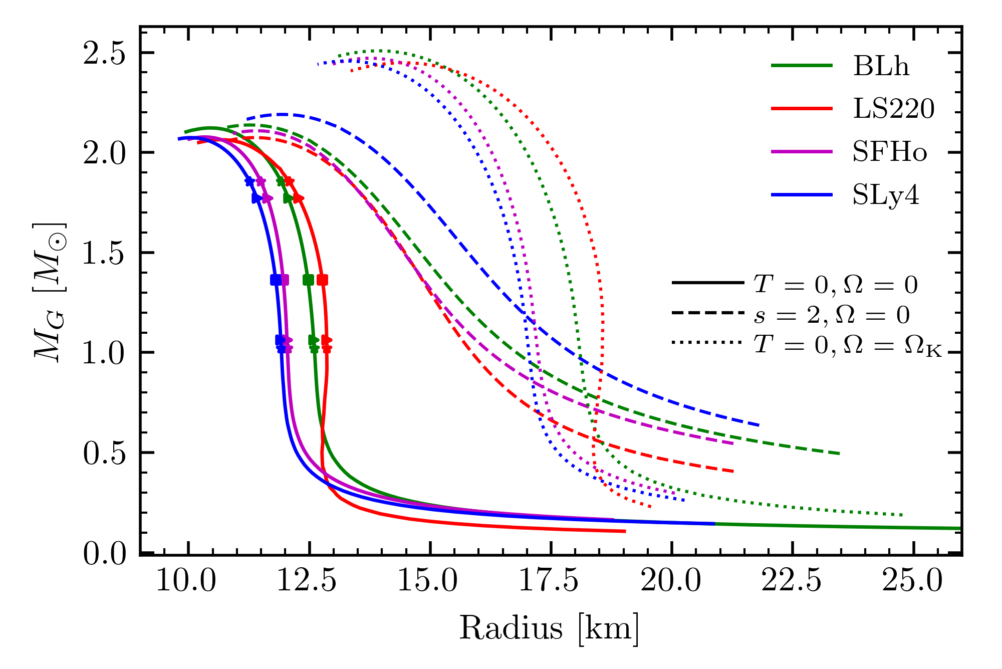
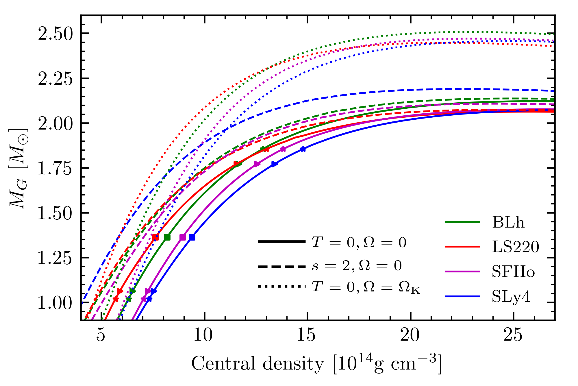
Figure 1: Equilibrium NS sequences obtained for the different EOS used in this work. Solid lines correspond to irrotational, $T=0$ configurations; dashed lines to irrotational, isentropic ($s=2~{}{k_{\rm B}~{}{\rm baryon^{-1}}}$) configurations; dotted lines represent $T=0$, rigidly rotating NS spinning at the mass sheeding limit ($\Omega=\Omega_{K}$). Left: gravitational mass versus radius (equatorial for rotating NS). Right: gravitational mass versus central density. Markers along the cold, nonrotating sequences indicate the NSs used in this work: squares, triangles and stars refer to $q=1,1.67,1.8$ binaries, respectively.

Fundamental differences in the EOS models translate in different NS structures. For cold, non-rotating NSs, the considered EOS can support maximum masses in the range $M_{\text{max}}^{\text{TOV}}\sim 2.06-2.10M_{\odot}$, while the predicted radii of a 1.4$M_{\odot}$ NS lay in the range $R_{1.4}\sim 11.78-12.74$ km. More specifically, LS220, SFHo, SLy4-SRO, and BLh EOS have $M_{\text{max}}^{\text{TOV}}$ of 2.04, 2.06, 2.06, and 2.10 $M_{\odot}$, and $R_{1.4}$ of 12.8, 12.0, 11.9, and 12.5 km, respectively. The predicted maximum NS masses and the 1.4$M_{\odot}$ NS radii are all compatible at one-sigma level with the recent detection of an extremely massive millisecond pulsar Cromartie et al. (2019) and with results obtained by the NICER collaboration Miller et al. (2019); Riley et al. (2019), although being systematically on the lower side. Note that EOS allowing NS radii $R_{1.4}\gg 13$ km are currently disfavoured by both GW BNS and X-ray pulsar observations Abbott et al. (2019a); Miller et al. (2019); Riley et al. (2019).

Finite temperature effects introduce additional pressure support. On the one hand, for the typical central entropies expected for nuclear matter during a BNS merger ($s\lesssim 2{k_{\rm B}}/{\rm baryon}$), this additional support is not sufficient to significantly alter the maximum TOV mass Kaplan et al. (2014) or the central baryon density due to the large degree of degeneracy of matter above saturation density. On the other hand, thermal effects can provide a more significant impact for matter at lower densities, increasing the NS radius. In Fig. 1 we report equilibrium sequences in the mass-radius and mass-central density plane obtained for the EOS used in this work, considering both a cold (continuous lines) and an isentropic (dashed lines) EOS with $s=2~{}{k_{\rm B}~{}{\rm baryon^{-1}}}$. Due to thermal effects, $R_{1.4}$ increases by the $15.6\%$ for the LS220 EOS and $36.4\%$ for the SLy4 EOS. while for the BLh and the SFHo EOS the variation is $\sim 21-22\%$. The different relative impacts on the NS radius clearly correlate with the different values of the nucleon effective mass.

Rotational support also increases the maximum NS mass. For example, in the limiting case of rigid rotation at the Keplerian limit, the maximum NS mass is increased by $\sim 20\%$ for all EOS models, as visible in Fig. 1, dotted lines. Since this affects the whole star, the NS radius is typically increased by $\sim 40\%$, but at the same time the central density is decreased by a similar amount, if one compares non-rotating and Keplerian NSs of identical masses. These properties emphasizes the importance of using the full EOS (i.e. including thermal effects) in merger simulations. Thermal (and composition, see (Kaplan et al., 2014)) effects are indeed key to quantify the prompt collapse dynamics, mass-shedding in the remnant and disc properties.

3 Simulations

3.1 Methods

We construct initial data for irrotational binaries in quasi-circular orbit solving the constraint equations of 3+1 general relativity in presence of a helical Killing vector and under the assumption of a conformally flat metric Gourgoulhon et al. (2001). The equations are solved with the pseudo-spectral multidomain approach implemented in the Lorene library . The EOS used for the initial data are constructed from the minimum temperature slice of the EOS table employed for the evolution assuming neutrino-less beta-equilibrium. Initial data have a residual eccentricity of ${\sim}0.01$ which is radiated away before merger, e.g. Thierfelder et al. (2011b).

The initial data are then evolved with the 3+1 Z4c free-evolution scheme for Einstein’s equations Bernuzzi & Hilditch (2010); Hilditch et al. (2013) coupled to general relativistic hydrodynamics. For the latter, we use the WhiskyTHC code Radice & Rezzolla (2012); Radice et al. (2014b, a) that implements the approximate neutrino transport scheme developed in Radice et al. (2016, 2018d) and the general-relativistic large eddy simulations method (GRLES) for turbulent viscosity Radice (2017). The interactions between the fluid and neutrinos are treated with a leakage scheme in the optically thick regions Ruffert et al. (1996); Rosswog & Liebendoerfer (2003); Neilsen et al. (2014) while free-streaming neutrinos are evolved according to the M0 scheme Radice et al. (2018d). The latter is a computationally efficient scheme that incorporates an approximate treatment of gravitational and Doppler effects, is well adapted to the geometry of BNS mergers and free of the radiation shock artifact that plagues the M1 scheme Foucart et al. (2018). The turbulent viscosity in the GRLES is parametrized as $\sigma_{T}=\ell_{\rm mix}c_{s}$, where $c_{s}$ is the sound speed and $\ell_{\rm mix}$ is a free parameter sets the intensity of the turbulence. For the simulations of this work $\sigma_{T}$ is prescribed as a function of the rest-mass (baryon) density using the results of the high-resolution general relativistic magnetohydrodynamics simulations results of a NS merger of Kiuchi et al. (2018). A detailed description of the model can be found in Radice (2020); simulations with this model are also presented in Perego et al. (2019); Nedora et al. (2019).

We remark that the GRLES method introduces parabolic terms for which there is no maximum characteristic velocity. However, parabolic equations still have an effective, wavelength dependent, propagation speed Weymann (1967); Kostadt & Liu (2000). Accordingly, only disturbances that have spatial scale that are small compared to the mixing length parameter are propagated with an effective velocity larger than the speed of light. These modes are absent in our simulations because the mixing length is always set to be smaller than the minimum grid scale in the simulation. Indeed, the GRLES method becomes invalid precisely when the mixing length becomes comparable with the grid scale, which would correspond to turbulent motion on a scale that is resolved in the simulations and should be included directly, not through a subgrid model. This is also the reason why it is possible to integrate the GRLES equations using an explicit time integration scheme. Moreover, it is possible to show that in the long wavelength and low frequency limit that is relevant for us, the solution of the parabolic model are always arbitrarily close to those of an associated hyperbolic model obtained with the introduction of relaxation terms Nagy et al. (1994). In other words, the parabolic and the (significantly more complex) hyperbolic models of turbulent viscosity should give the same results in our context.

WhiskyTHC is implemented within the Cactus Goodale et al. (2003); Schnetter et al. (2007) framework and coupled to an adaptive mesh refinement driver and a metric solver. The spacetime solver is implemented in the CTGamma code Pollney et al. (2011); Reisswig et al. (2013a), which is part of the Einstein Toolkit Loffler et al. (2012). We use fourth-order finite-differencing for the metric’s spatial derivatives method of lines for the time evolution of both metric and fluid. We adopt the optimal strongly-stability preserving third-order Runge-Kutta scheme Gottlieb & Ketcheson (2009) as time integrator. The timestep is set according to the speed-of-light Courant-Friedrich-Lewy (CFL) condition with CFL factor $0.15$. While numerical stability requires the CFL to be less than $0.25$, the smaller value of $0.15$ is necessary to guarantee the positivity of the density when using the positivity-preserving limiter implemented in WhiskyTHC.

The computational domain is a cube of $3,024$ km in diameter whose center is at the center of mass of the binary. Our code uses Berger-Oliger conservative AMR Berger & Oliger 1984 with sub-cycling in time and refluxing Berger & Colella (1989); Reisswig et al. (2013b) as provided by the Carpet module of the Einstein Toolkit Schnetter et al. (2004). We setup an AMR grid structure with 7 refinement levels. The finest refinement level covers both NSs during the inspiral and the remnant after the merger and has a typical resolution of $h\simeq 246$ m (grid setup named LR), $h\simeq 185$ m (SR) or $123$ m (HR).

Black-hole formation is indicated by the appearance of an apparent horizon (AH) that is computed with the module AHFinderDirect Thornburg (2004). With the gauge conditions employed in the simulations, the BH is formed and simulated as a puncture Thierfelder et al. (2011a); Dietrich & Bernuzzi (2015). In a first series of simulations, the AH finder could not find an AH in the simulations using the GRLES scheme. We have thus repeated them and found that in those cases was necessary to (i) increase the number of more guess spheres for the finder, and (ii) switch off the GRLES scheme in regions with $\alpha<0.1$ in order to compute the AH robustly. The latter is analogous to the ”hydro-excision” implemented in many codes to facilitate AH location. This way we obtained horizon data for all the LR and most of the SR simulations. We could not rerun the HR simulations for which the AH was not found initially for lack of computational resources. Finally, the employed grid structure is not optimal to follow the dynamics of the BH+disc remnant; thus simulations are stopped ${\sim}5-10$ ms after BH formation.

3.2 BNS Models

We consider 10 binaries with fixed chirp mass ${\cal M}_{c}\simeq 1.188M_{\odot}$ and simulate them at different resolutions. The chirp mass is ${\cal M}_{c}=M\nu^{3/5}$ where $\nu=M_{A}M_{B}/M^{2}=q/(1+q)^{2}$. The main properties of the BNS initial data are summarized in Tab. 1. We simulated the equal mass case and mass ratio $q=1.67$ for all the EOS with the GRLES scheme. The highest mass ratio simulated are $q=1.8$ for the BLh and SLy EOS. A subset of models were simulated also without turbulent viscosity to directly assess its impact on the merger dynamics and on the ejecta properties. The initial separation between the NS is set to $45\,{\rm km}$, corresponding to ${\sim}4-6$ orbits to merger. Note that similar equal mass LS220 and SFHo BNS were already presented in Perego et al. 2019, but the mass here is slightly larger. An equal mass SLy4 without turbulent viscosity was instead presented in Endrizzi et al. (2020).

The table also reports the reduced tidal parameter Favata (2014)

$$\tilde{\Lambda}=\frac{16}{13}\frac{(M_{\text{A}}+12M_{\text{B}})M_{\text{A}}^{4}}{M^{5}}\Lambda_{\text{A}}+(A\leftrightarrow B)\ .$$ (1)

where $\Lambda_{i}\equiv 2/3k^{i}_{2}(GM_{i}/R_{i}c^{2})^{5}$, with $i=(A,B)$, are the dimensionless quadrupolar tidal polarizability parameters of the individual stars Flanagan & Hinderer (2008); Damour & Nagar (2010), $k^{i}_{2}$ the dimensioless quadrupolar Love numbers Damour (1983); Hinderer (2008); Damour & Nagar (2009); Binnington & Poisson (2009), and $(M_{i},R_{i})$ the NS mass and radius. The tidal parameter enters at leading-order the post-Newtonian dynamics and it is directly measurable from the GW Damour & Nagar (2010); Damour et al. (2012b). Its range for fiducial BNS systems is $\tilde{\Lambda}\approx(10,2000)$, where softer EOS, larger masses and higher mass-ratios result in smaller values of $\tilde{\Lambda}$. It can be used as a measure of the binary compactness and correlates with prompt collapsed remnant and disc masses Radice et al. (2018b); Zappa et al. (2018).

Table 1: BNS models considered in this work. $M_{\text{max}}^{\text{TOV}}$ is the maximum gravitational mass for a TOV solution with the specified EOS, $C^{\text{TOV}}_{\text{max}}=GM_{\text{max}}^{\text{TOV}}/Rc^{2}$ is the compactness relative to the maximum mass configuration. $M_{b}$ is the total baryonic mass of the BNS, $M_{A}$ and $M_{B}$ are the gravitational masses of the individual NSs at infinite separation, $q$ is the mass ratio $M_{A}/M_{B}\geq 1$ and $\tilde{\Lambda}$ is the tidal parameter of Eq. 1. $f_{\text{GW}}(0)$ is the initial GW frequency. Masses are expressed in $M_{\odot}$, frequencies in Hertz.

EOS	$M_{\text{max}}^{\text{TOV}}$	$C^{\text{TOV}}_{\text{max}}$	$M_{b}$	$M_{A}$	$M_{B}$	$q$	$M$	$\tilde{\Lambda}$	$f_{\text{GW}}(0)$
	$[M_{\odot}]$		$[M_{\odot}]$	$[M_{\odot}]$	$[M_{\odot}]$		$[M_{\odot}]$		$[\text{Hz}]$
BLh	$2.103$	$0.298$	$2.98$	$1.364$	$1.364$	$1.0$	$2.728$	$511$	$565$
BLh	$2.103$	$0.298$	$3.14$	$1.772$	$1.065$	$1.67$	$2.837$	$506$	$574$
BLh	$2.103$	$0.298$	$3.21$	$1.856$	$1.020$	$1.8$	$2.876$	$504$	$576$
LS220	$2.044$	$0.284$	$2.98$	$1.364$	$1.364$	$1.0$	$2.728$	$639$	$565$
LS220	$2.044$	$0.284$	$3.14$	$1.772$	$1.065$	$1.67$	$2.837$	$638$	$574$
SFHo	$2.059$	$0.294$	$3.00$	$1.364$	$1.364$	$1.0$	$2.728$	$395$	$565$
SFHo	$2.059$	$0.294$	$3.16$	$1.772$	$1.065$	$1.67$	$2.837$	$386$	$573$
SLy4	$2.055$	$0.303$	$3.00$	$1.364$	$1.364$	$1.0$	$2.728$	$361$	$565$
SLy4	$2.055$	$0.303$	$3.17$	$1.772$	$1.065$	$1.67$	$2.837$	$358$	$574$
SLy4	$2.055$	$0.303$	$3.24$	$1.856$	$1.020$	$1.8$	$2.876$	$357$	$577$

4 Merger Dynamics & Remnant

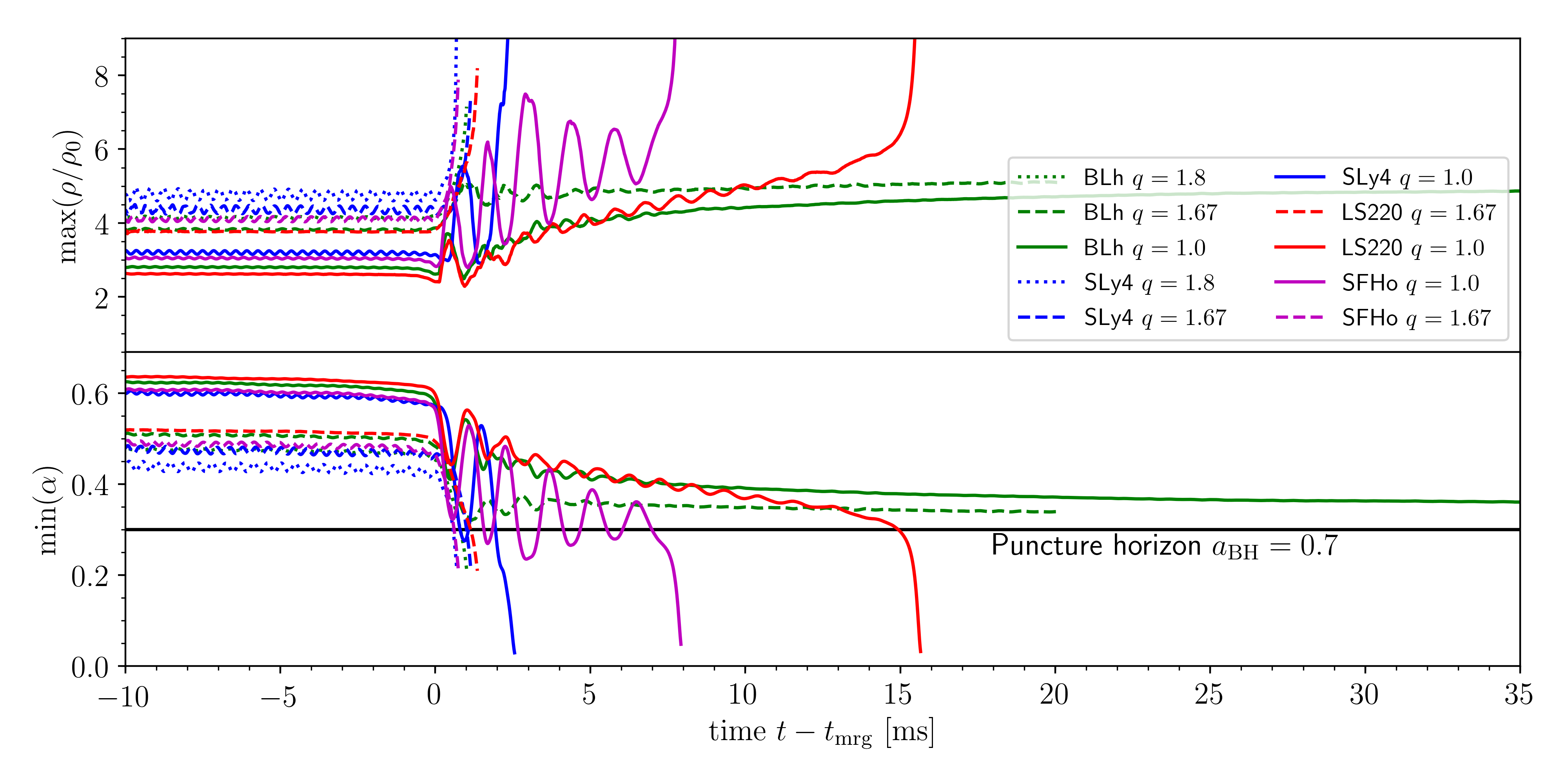
Figure 2: Evolution of the maximum density (normalized to nuclear saturation density) and of the minimum lapse in all simulations. The horizontal line indicates the value of the lapse at the horizon for a puncture with the indicated dimensionless spins (Cf. Tab. 2). Data refer to simulations with turbulent viscosity and resolution SR.

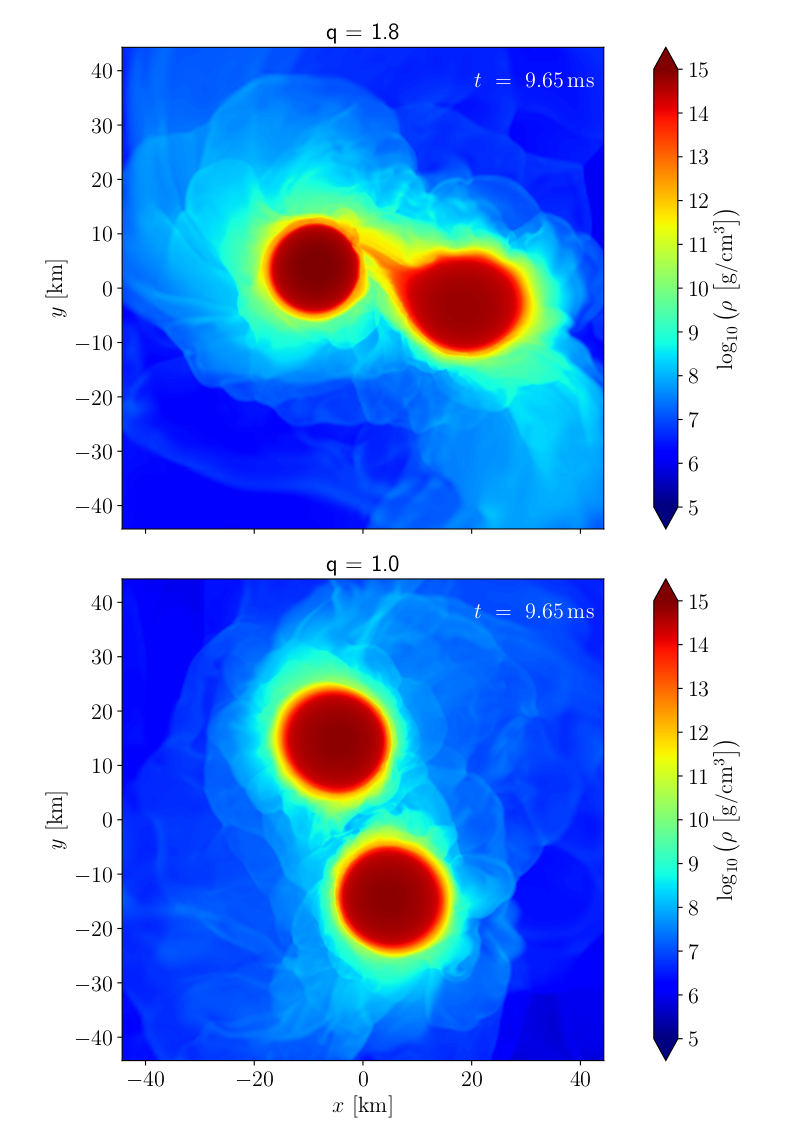
Figure 3: Snapshots of premerger dynamics for BLh $q=1.8$ (top) and $q=1.0$ (bottom) simulations. Shown is the rest-mass density in the orbital plane at ${\sim}9$ ms corresponding to the third orbit from the beginning of the simulations and $2$ orbits to the moment of merger. The companion in the $q=1.8$ BNS is tidally disrupted and a significant accretion onto the primary is taking place. Accretion starts approximately after one orbits from the beginning of the simulations.

Starting at a GW frequency of ${\sim}570$ Hz, the binaries revolve for ${\sim}$4-6 orbits before reaching the moment of merger. The latter is defined as the peak amplitude of the $(2,2)$ GW mode and marks the end of the chirp signal. A summary of the merger dynamics for all the runs is given in Fig. 2, which shows the maximum mass density (fluid frame) and the minimum of the lapse function, $\alpha$. Black-hole formation is indicated by the lapse dropping below $\alpha\lesssim 0.3$. Note that the 1+log slicing of the spherical puncture has lapse function at the horizon $\alpha_{\text{AH}}\simeq 0.376$ Hannam et al. (2007, 2008), but punctures formed in our simulations have dimensionless spins ${\sim}0.7$ for which $\alpha_{\text{AH}}\simeq 0.3$ (See Appendix A). At the same time the lapse decreases below $\alpha_{\text{AH}}$, the maximum density increases beyond $6\rho_{0}$ and it is then unresolved on the grid due to the gauge conditions Thierfelder et al. (2011a).

The remnants of BLh $q=1.8$, LS220 $q=1.67$, SFho $q=1.67$ and SLy4 $q=1,1.67,1.8$ collapse to BH within ${\sim}$2-3 ms from merger. We call prompt BH collapse mergers those in which the NS cores collision has no bounce but instead the remnant immediately collapse at formation, see Tab. 2. This usually happens within 1-2 ms from the moment of merger and can be identified by the maximum density monotonically increasing to the collapse, Fig. 2. Note that this definition of prompt collapse implies negligible shocked dynamical ejecta because the bulk of this mass emission comes precisely from the (first) core bounce Radice et al. (2018d). The BH masses of the prompt collapsed remnants are $M_{\text{BH}}\simeq 2.49,2.44,2.45,2.47,2.52M_{\odot}$ for BLh $q=1.8$, LS220 $q=1.67$, SFho $q=1.67$ and SLy4 $q=1.67,1.8$ respectively. The BH spins are $a_{\text{BH}}\simeq 0.66,0.7,0.68,0.69,0.66$. The remnants of LS220, SFHo and SLy $q=1$ also form BH within the simulated time and they have $M_{\text{BH}}=2.41,2.41,2.38$ and spins $a_{\text{BH}}=0.5,0.75,0.76$ respectively. The SLy4 $q=1$ merger was simulated in Endrizzi et al. (2020) without viscosity, and in that case the remnant survives for ${\sim}10$ ms. The earlier collapse here is a consequence of the angular momentum redistribution by the subgrid model for turbulent viscosity Radice (2017). Overall these results for the BH spins consistently indicate an upper limit on the BH rotation of $a_{\text{BH}}\lesssim 0.8$, also when including $q\sim 2$ BNS Kiuchi et al. (2010); Bernuzzi et al. (2014, 2016); Dietrich et al. (2017). In the following, we first discuss the details of the BH formation highlighting the effect of high mass ratio and the main differences with respect to the (well-studied) equal mass cases. Then, we discuss the properties of the remnant discs.

For comparable masses the NS cores enter in contact before reaching the moment of merger Thierfelder et al. (2011b) and the last two 2-3 GW cycles before the amplitude’s peak are emitted by the cores collision and remnant formation. At high mass ratios, a new effect is the tidal disruption of the companion and its accretion onto the primary NS. This has been reported also in previous simulations with a stiff polytropic EOS Dietrich et al. (2017), and we confirm it here for softer and microphysical EOS. As a representative example we show in Fig. 3 the cases of BLh $q=1$ vs. $q=1.8$. The accreting material has initially low temperatures but as soon as the accretion becomes more massive and faster the temperature raises. At approximately the time of the snapshot the accreting material shocks against the primary NS core and there the temperature raises up to ${\sim}100$ MeV. As a consequence of this shock, some material becomes unbound, although the exact amount of ejecta cannot be confidently measured in the simulations (see Sec. 6).

The new aspect highlighted by our simulations is the dynamics of prompt collapse for high mass-ratio BNS. In a $q\sim 1.5-2$ binary the tidal disruption and accretion of the companion NS onto the massive primary NS can drive the remnant unstable and causes a prompt collapse to BH. The process is shown in Fig. 4 (top panels) in a 3D volume rendering of the rest mass density for the representative case of the BLh EOS. The BLh $q=1.8$ has a rather massive primary NS with $M_{A}=1.856M_{\odot}$ as compared to the maximum TOV mass for the BLh EOS ($M_{\text{max}}^{\text{TOV}}=2.103M_{\odot}$), and a companion NS of small compactness ($M_{B}=1.020$ and $C_{B}\simeq 0.12$.) The companion NS is almost completely destroyed by tidal effects and its accretion results in the prompt formation of a BH surrounded by a massive accretion disc (see below). By contrast the lower mass-ratio and equal-mass binaries with the same chirp mass produce a less compact remnant and none of them collapse to the end of the simulated time (middle and bottom panels). Note that the equal mass BLh was evolved beyond $80$ ms postmerger. We checked with a sequence of simulations at intermediate mass ratios that the behavior is continuous in the mass ratio parameter (See Appendix B).

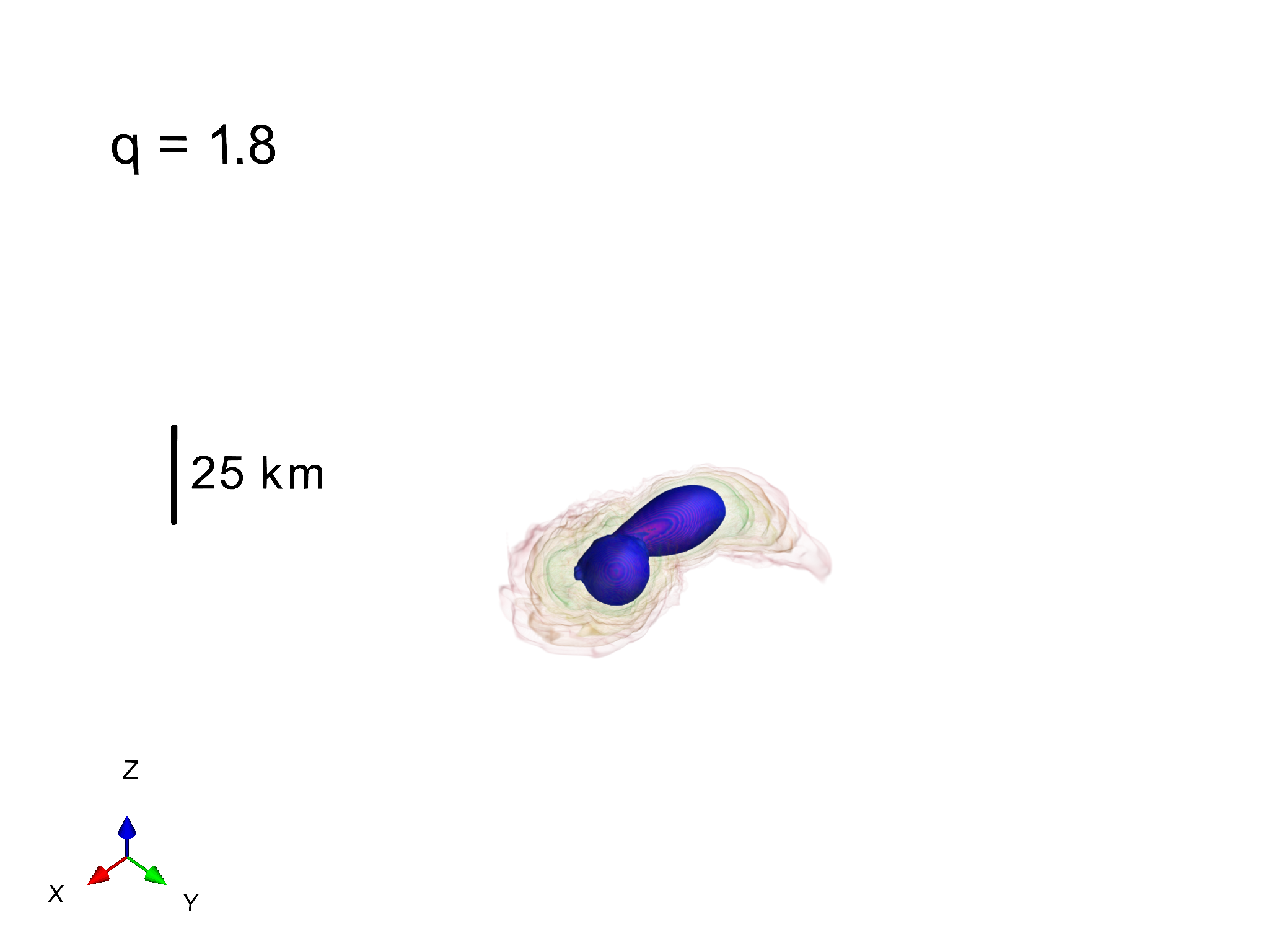
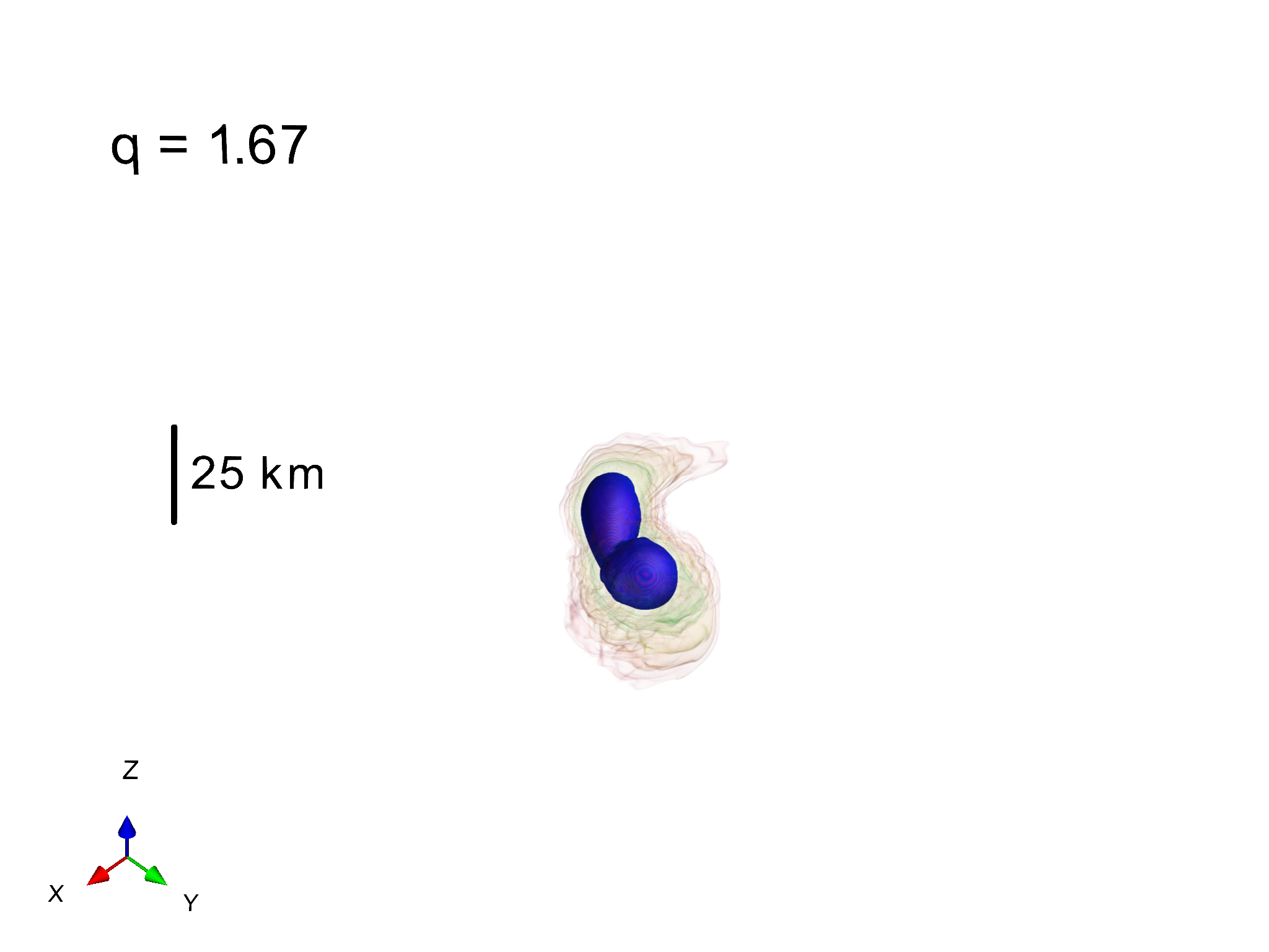
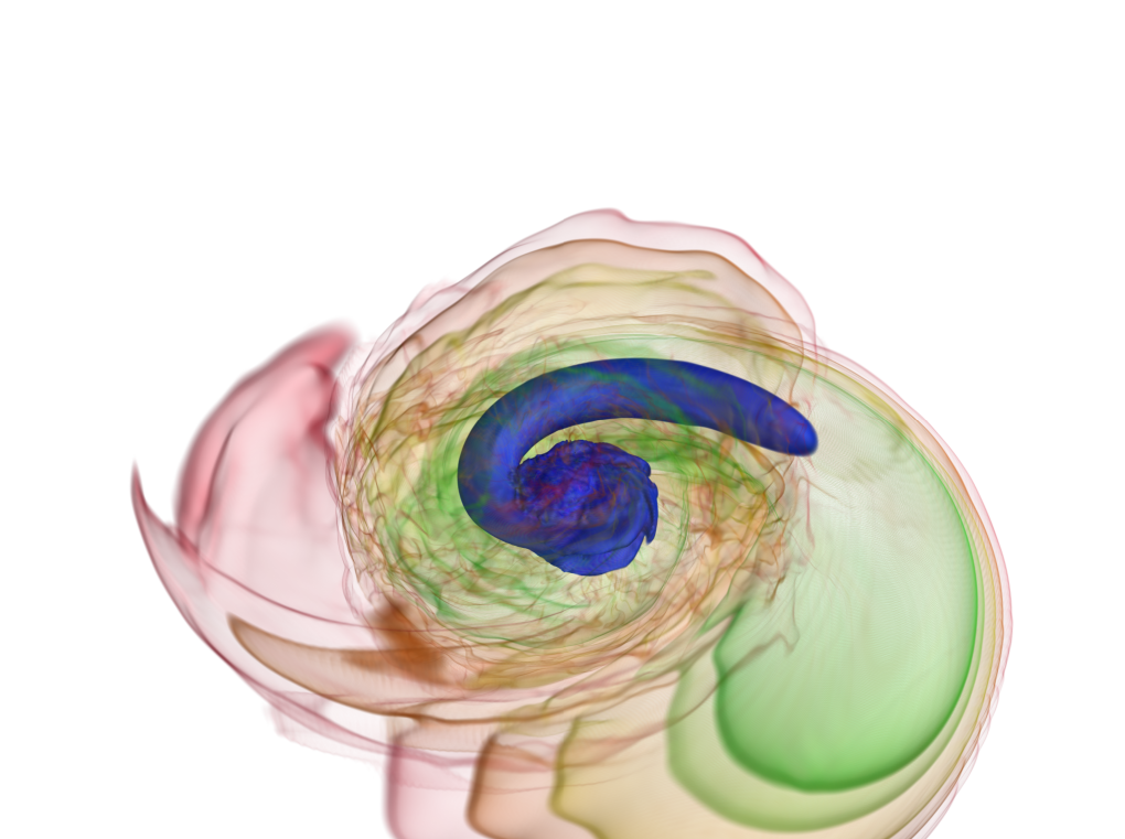
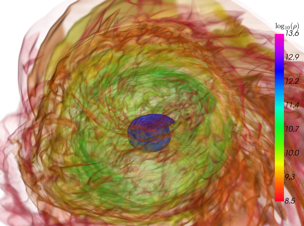
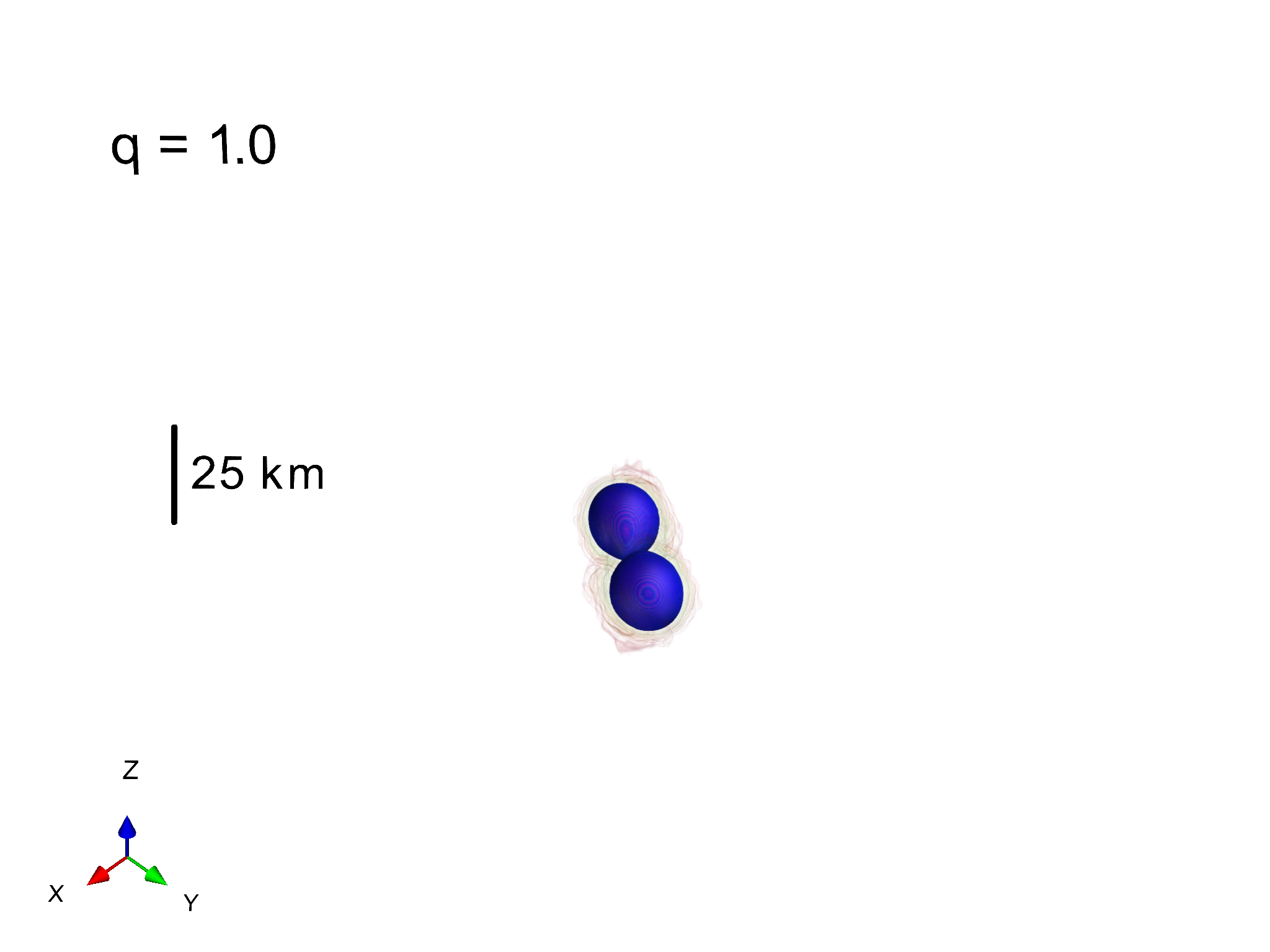
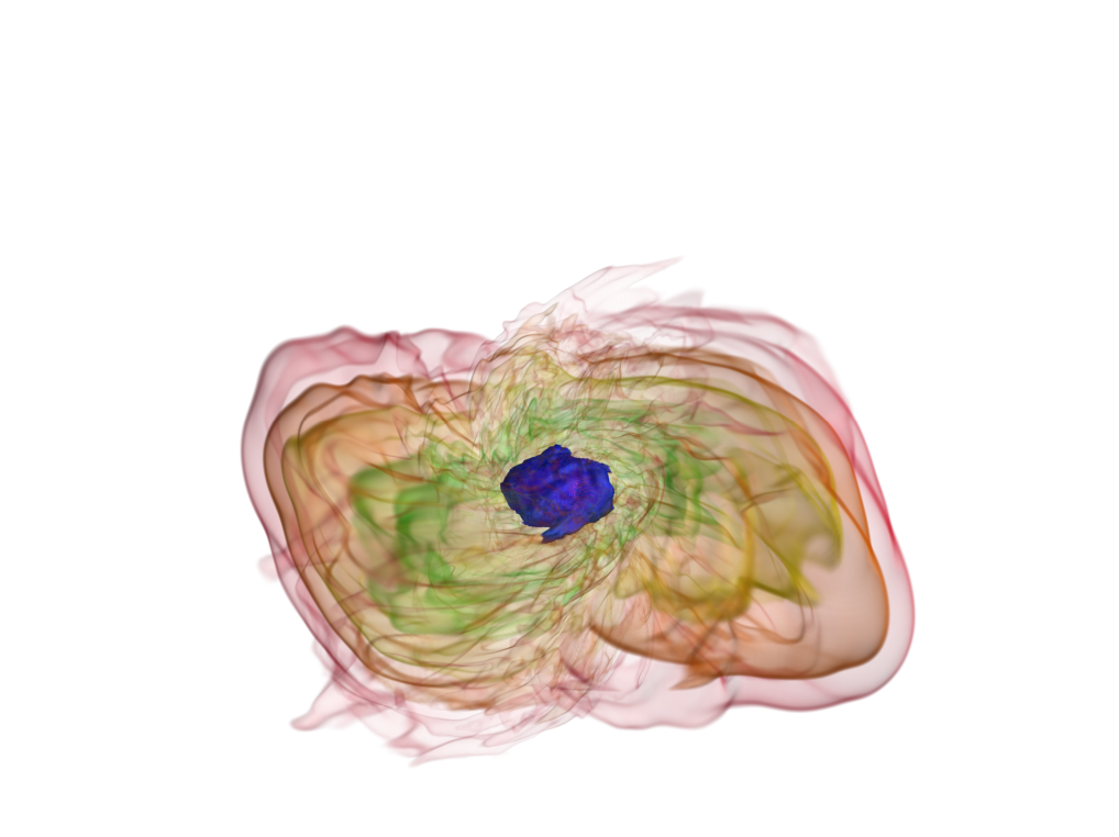
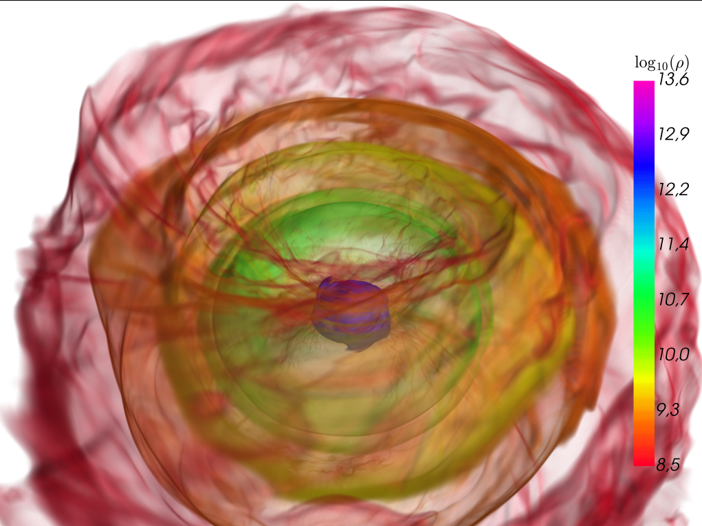
Figure 4: 3D volume rendering of the rest mass density $\rho$ in g cm^-3 expressed in logarithmic scale for the BLh models. Each column represents a different time inside the simulation: merger time (left), early postmerger ($\sim 2{\rm ms}$, middle) and later stages ($\sim 10{\rm ms}$, right). In each row we show a different mass ratio $q=M_{A}/M_{B}$: $q=1.8$ (top), $q=1.67$ (middle) and $q=1.0$ (bottom). The BH apparent horizon is shown as a bright green isosurface of the lapse function $\alpha=\alpha_{\text{AH}}$.

Comparing our results to the numerical-relativity–based models of prompt collapse available in the literature we find that the current models fail to predict the behavior at high mass ratio. This is not surprising since all the models are calibrated using almost exclusively comparable masses simulations. In particular, the prompt collapse model proposed in Bauswein et al. (2013a) predicts prompt collapse for BNS with masses exceeding a threshold mass

$$M>M_{\text{thr}}=k_{\text{thr}}M_{\text{max}}^{\text{TOV}}\ ,$$ (2)

where the quantity $k_{\text{thr}}$ can be expressed in an approximately EOS-independent way in terms of the maximum mass TOV compactness. Using also data from Hotokezaka et al. (2011); Zappa et al. (2018); Koeppel et al. (2019), a best fit expression was derived in Agathos et al. (2020):

$$k_{\text{thr}}(C_{\text{max}})=-(3.29\pm 0.23)\,C_{\text{max}}+(2.392\pm 0.064)\ .$$ (3)

The above model does not include any dependence on the mass ratio and predicts that all models simulated in our work would produce a NS remnant, except the BLh $q=1.8$. The prediction is shown as solid line in the $M$ vs. $C_{\text{max}}$ diagram in Fig. 5; prompt collapse would be expected for BNS above the solid line. A possible way to improve the criterion in Eq. (2) is to correct the threshold mass by a function of the mass ratio, $f(\nu)$. For example, one could look for a criterion based on the chirp mass. Letting

$$M_{\text{thr}}\mapsto M_{\text{thr}}f(\nu)=M_{\text{thr}}(4\nu)^{3/5}\ ,$$ (4)

lowers the threshold and approximately reproduces our results (dashed and dotted lines in the Fig. 5.) The limited data points available do not allow us more quantitative studies or fitting.

Another criterion for prompt collapse that is independent on the EOS is based on the value of the tidal parameter Zappa et al. (2018); Agathos et al. (2020)

$$\tilde{\Lambda}>\tilde{\Lambda}_{\text{thr}}\sim 338-386\ .$$ (5)

Note that the $\tilde{\Lambda}$ parameter contains the mass ratio dependence, and for $q\gg 1$

$$\tilde{\Lambda}=\frac{16}{13}\frac{M_{A}^{5}}{M^{5}}\left(1+12\dfrac{M_{B}}{M_{A}}\right)\Lambda_{A}+(A\leftrightarrow B)\approx q^{5}\ .$$ (6)

Comparing to our data, we find that it predicts correctly the prompt collapse of the highest simulated mass ratio for SFHo and SLy4, but fails for the LS220 and BLh. This is also expected since $\tilde{\Lambda}$ does not account for tidal disruption but only measures the binary compactness [Cf. discussion in Appendix A in Breschi et al. (2019).]

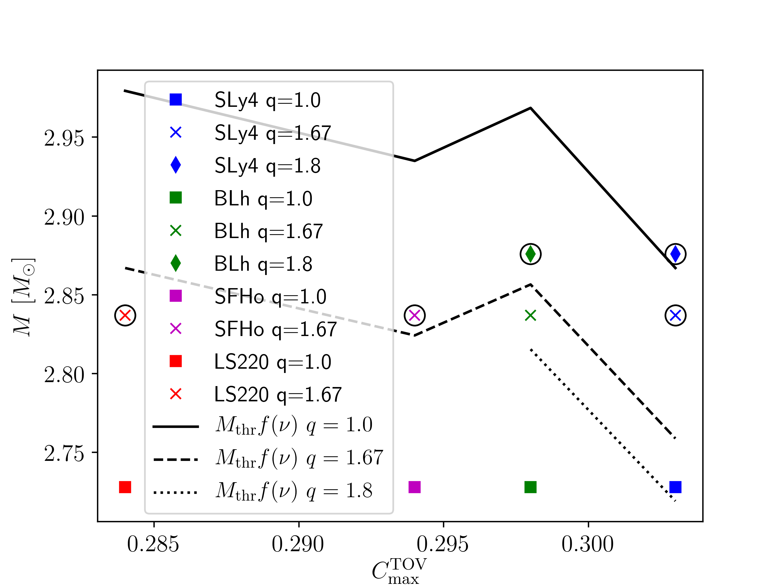
Figure 5: Masses of simulated BNS as function of the TOV maximum compactness as predicted by the zero-temperature EOS. Prompt collapsing remnant are marked with additional black circles. The solid line is the mass threshold given by Eq. 2 ($q$-independent): binaries above the line are predicted to collapse. The dashed and solid lines are the thredshold model modified by the mass-ratio correction in Eq. 4. The plot refers to simulations with turbulent viscosity only.

Table 2: Remnant properties. For each simulation the table reports BH properties (if applicable) and estimates for the disc properties. The BH properties are all reported from simulations at SR except the BLh $q=1.8$ and LS220 $q=1$ for which only LR data are available. The relative differences between LR and SR data are ${\sim}1$% and ${\sim}3$% for mass and spin respectively. The disc mass is measured at the time it is maximum. For remnant collapsing to BH this corresponds to the mass at formation that later accretes onto the BH. For NS remnants the disc can also increase its mass over time acquiring matter expelled from the NS. Note the numbers in this table are reported from simulations at resolutions LR or SR as available, and are affected by uncertainties up to 20-40%.

EOS	$q$	Prompt BH	$M_{\text{BH}}$	$a_{\text{BH}}$	$M_{\text{disc}}^{\text{max}}$ $[M_{\odot}]$
BLh	1.0	✗	N.A.	N.A.	0.15
BLh	1.67	✗	N.A.	N.A.	0.29
BLh	1.8	✓	2.49	0.66	0.17
LS220	1.0	✗	2.41	0.55	0.12
LS220	1.67	✓	2.44	0.70	0.16
SFHo	1.0	✗	2.38	0.75	0.08
SFHo	1.67	✓	2.45	0.68	0.14
SLy4	1.0	✗	2.41	0.76	0.05
SLy4	1.67	✓	2.47	0.69	0.10
SLy4	1.8	✓	2.52	0.66	0.15

Let us now discuss disc formation, evolution and properties. Following a common convention, we define disc the baryon material either outside the BH’s apparent horizon or the one with densitites $\rho\lesssim 10^{13}$ $\mathrm{g~{}cm^{-3}}$ around a NS remnant. The baryonic mass of the discs are computed as volume integrals of the conserved rest-mass density $D=\sqrt{\gamma}~{}W\rho$ from 3D snapshots of the simulations in postprocessing ($\gamma$ is the 3-metric’s determinant and $W$ the Lorentz factor). Estimates for the disc masses are reported in Tab. 2. The disc mass is reported as measured at the time when it is maximum during the simulation. For remnant collapsing to BH this can be interpreted as the mass at BH formation, since the disc mass can only decrease with time due to accretion. For NS remnants the disc (remnant at lower densitites) can also increase its mass over time as it acquires matter expelled from the higher densities shells.

Examples of the disc mass evolutions for different remnants are shown in Fig. 6. Note that we show the BLh $q=1.8$ and LS220 $q=1$ simulations at resolution SR but without turbulent viscosity and the $q=1.67$ with viscosity but at LR because these are the longer dataset available to us (see below for a discussion about turbulence.)

In the case of comparable mass BNS the accretion disc is formed during and after the merger. As time evolves, if the remnant does not collapse, it continuosly shedes mass and angular momentum increasing the mass of the disc and generating outflows Radice et al. (2018a); Nedora et al. (2019). This is why in Fig. 6 the accretion disc mass is increasing with time for these binaries. These processes terminate with BH formation, which is accompanied by the rapid accretion of a substantial fraction of the disc. An important consequence is that, in the case of comparable mass ratio binaries, prompt BH formation results in very small accretion disc masses Radice et al. (2018b); Kiuchi et al. (2019), because the mechanism primarily responsible for the formation of the disc is shut off immediately in these cases.

In high mass ratio BNS mergers the companion star is tidally disrupted (Fig. 4). In these cases, the bulk of the accretion disc is constituted by the tidal tail, which is for the most part still gravitationally bound to the remnant. This tail is launched prior to merger. So massive accretion discs are possible even if prompt BH formation occurs (see also Kiuchi et al. 2019.) In general, high $q$ binaries are found to generate more massive discs than binaries with the same chirp mass but lower $q$ Shibata et al. (2003); Shibata & Taniguchi (2006); Kiuchi et al. (2009); Rezzolla et al. (2010); Dietrich et al. (2017). The postmerger evolution of these discs is also very different. While in the massive NS case the central object pushes material into the disc and drives outflows, in the case of high mass-ratio binaries forming BHs the fallback of the tidal tail perturbs the disc and drives rapid accretion onto the BH as evinced by the rapid decrease of the disc masses with time shown in Fig. 6.

These different formation mechanisms are imprinted in the structure and composition of the discs formed in comparable and very unequal mass binaries, as shown in Fig. 7. In the case of equal mass binaries, the disk is composed of material squeezed out of the collisional interface between the NSs Radice et al. (2018d), see also Fig. 4. This matter is heated to temperatures of tens of MeV before being pushed out of the central part of the remnant, so its electron fraction is reset by pair processes Perego et al. (2019), see Fig. 7. Due to the absence of strong compression and shockes, the discs formed in high mass ratio binaries are initially colder and more neutron rich (Fig. 7). Since high-$q$ BNS mergers launch tidal tails to large radii, comparable mass-ratio binaries create discs that are initially more compact and have higher $Y_{e}$’s. Besides the mass ratio, the structure of the disc is also strongly dependent on the nature of the remnant. In the case of BH remnants, the discs are typically more compact and thin than those around massive NS remnants. In the latter case, because of the additional pressure support, the discs reach higher densities ${\sim}10^{13}~{}\mathrm{g~{}cm^{-3}}$ and become partly optically thick to neutrinos Perego et al. (2019); Endrizzi et al. (2020).

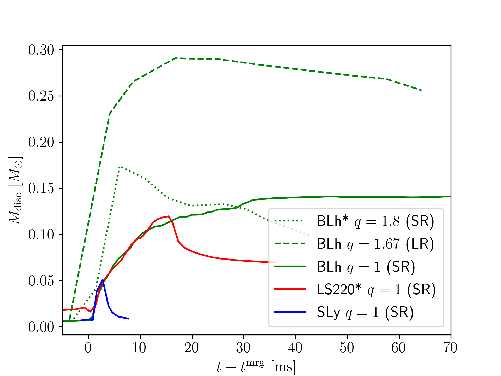
Figure 6: Evolution of the disc rest mass in representative remnants. The disc is defined as the remnant outside the apparent horizon if the remnant has collapsed to a BH or as the portion of the remnant whose rest mass density satisfies $\rho<10^{13}~{}\mathrm{g~{}cm^{-3}}$ otherwise.

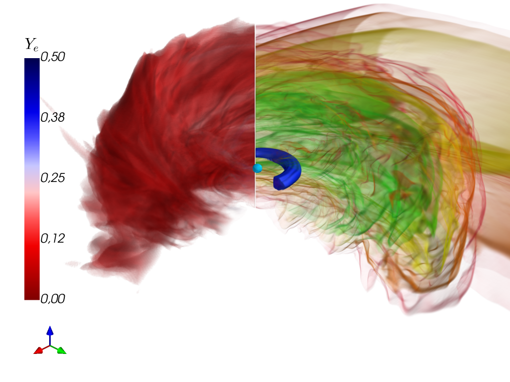
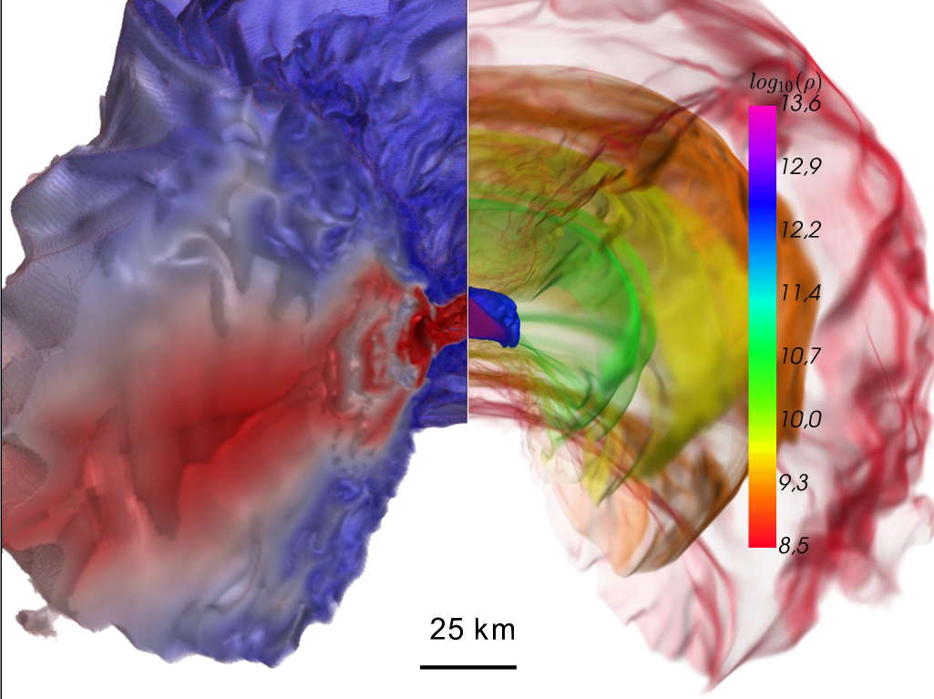
Figure 7: Volume rendering of density at the end of the BLh $q=1.8$ (left panel) and $q=1$ (right panel) simulations. In each panel, on the left we show the electron fraction distribution, while on the right we plot the rest mass density; for both quantities, we show only matter with densities $\rho\geq 3\times 10^{8}\mathrm{gcm}^{-3}$. The spatial scale is the same in the two panels.

5 Gravitational waves

Table 3: Gravitational-wave data extracted at the moment of merger from NR simulations presented in this work, expressed in dimensionless units according with the convention $G=c=M_{\odot}=1$. The energy $e_{b}^{\text{mrg}}$ and the angular momentum $j^{\text{mrg}}$ are defined from the gravitational wave data as: $e_{b}^{\text{mrg}}=E_{b}^{\text{mrg}}/(\nu M)$ and $j^{\text{mrg}}=J^{\text{mrg}}/(\nu M^{2})$. The following values have a numerical uncertainty of ${\sim}$5% due to the different grid resolutions.

EOS	$M$	$q$	$Mf^{\text{mrg}}_{22}$	$e_{b}^{\text{mrg}}$	$j^{\text{mrg}}$	$A_{\text{mrg}}/M$
BLh	2.728	$1.0$	0.02567	-0.05900	3.443	0.2566
BLh	2.837	$1.67$	0.01966	-0.05538	3.523	0.2110
BLh	2.876	$1.8$	0.01885	-0.05471	3.517	0.2014
LS220	2.728	$1.0$	0.02349	-0.05714	3.469	0.2465
LS220	2.837	$1.67$	0.01804	-0.05265	3.582	0.1986
SFHo	2.728	$1.0$	0.02581	-0.06099	3.404	0.2670
SFHo	2.837	$1.67$	0.02063	-0.05569	3.485	0.2100
SLy4	2.728	$1.0$	0.02649	-0.06087	3.413	0.2766
SLy4	2.837	$1.67$	0.02032	-0.05445	3.490	0.2097
SLy4	2.876	$1.8$	0.01998	-0.05693	3.478	0.1796

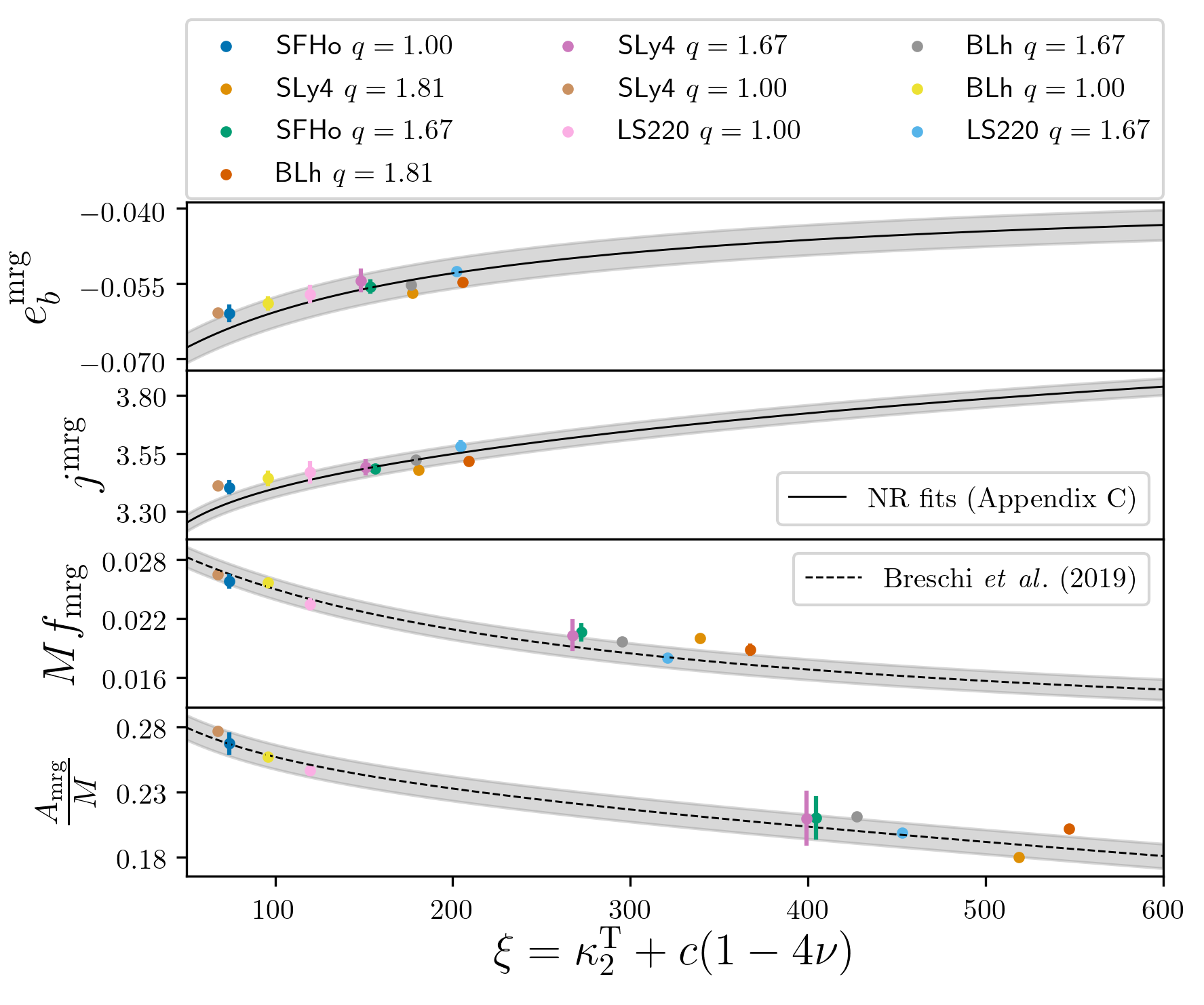
Figure 8: Comparison between GW data at moment of merger extracted from the simulations introduced in this work (and listed in Tab. 3) and fits calibrated using NR simulations with $q\leq 1.5$. The fits for energy and angular momentum are reported in Appendix C, while frequency and amplitude fits are from Breschi et al. (2019). The quantities $e_{b}^{\rm mrg}$ and $j^{\rm mrg}$ are defined from the GW data as $e_{b}^{\rm mrg}=E_{b}^{\rm mrg}/(\nu M)$ and $j^{\rm mrg}=J^{\rm mrg}/(\nu M^{2})$. The results extracted from high mass ratio simulations are consistent with the current fits in the limit of the uncertainties.

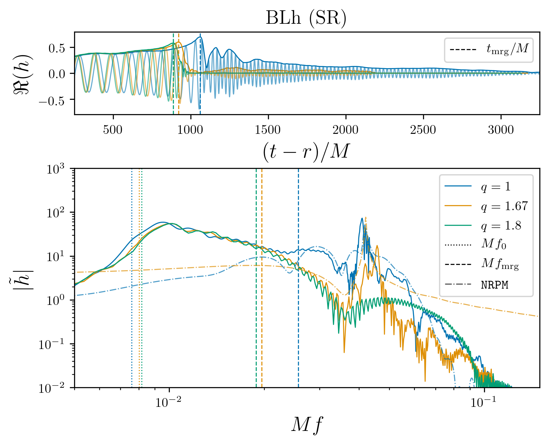
Figure 9: Example of GW signals. Amplitude and real part of the $(2,2)$ mode strains (top panel) and respective frequency-domain spectra (bottom panel) for the three simulations with BLh EOS at standard resolution. The vertical dashed lines mark the merger times, both in time- and frequency-domain, while the dotted lines in the bottom panel show the initial point of the simulations. The frequency-domain spectra are compared with NRPM postmerger model evaluated with the same physical values, except for the prompt-collapse case (BLh, $q=1.8$).

In this section we analyze the GW signals computed from the simulations. The latter are too short for a quantitative comparison with inspiral-merger models, e.g. Akcay et al. (2019). Hence, we focus on the merger and postmerger signal. The new simulations allow us to verify (and extend) the quasiuniversal relations characterizing the merger and study the postmerger waveform Bernuzzi et al. (2015b); Breschi et al. (2019).

Following Damour et al. (2012a) (see also Bernuzzi et al. 2012) we compute the reduced binding energy $e_{b}^{\text{mrg}}=E_{b}^{\text{mrg}}/(\nu M)$ and the angular momentum $j^{\text{mrg}}=J^{\text{mrg}}/(\nu M^{2})$ at the moment of merger from the multipolar GW. Those and other quantities at merger are approximately EOS-independent functions of the tidal parameter Bernuzzi et al. (2015a). To find these relations it is best to use, instead of $\tilde{\Lambda}$, the parameter

$$\kappa_{2}^{\text{T}}=\dfrac{3}{2}\left[\Lambda_{2}^{\text{A}}\left(\frac{M_{\text{A}}}{M}\right)^{4}M_{\text{B}}+(A\leftrightarrow B)\right]\ ,$$ (7)

determining both tidal dynamics and tidal waveform at leading post-Newtonian order Damour & Nagar (2010); Damour et al. (2012b). High mass-ratio effects are included by further considering the parametrization

$$\xi=\kappa_{2}^{T}+c(1-4\nu)\ ,$$ (8)

where $c$ is a fitting parameter Zappa (2018); Breschi et al. (2019). Binding energy, angular momentum and the waveform key quantities at merger are reported in Tab. 3 for all simulations. From the table one notices that the binding energy and the angular momentum increase (binding energy is less negative) as $\tilde{\Lambda}$ decreases and $q$ increases (Tab. 1); consequently the merger GW frequency and amplitude decreases. The dimensionless BH spin of the remnants is $a_{\text{BH}}\sim 0.7$ (Tab. 2), and it can be compared to the angular momentum available at merger considering its reduced value $j_{\text{BH}}(\nu)=a_{\text{BH}}\nu$. The angular momentum at merger is partly radiated in GW and partly gives the disc angular momentum and BH spin. For the $q=1.8$ prompt collapse remnants ($\nu\simeq 0.22959$, BLh and SLy4) we obtain $j_{\text{BH}}(0.22959)=0.66/0.22959\simeq 2.87$ to be compared to $j^{\text{mrg}}\simeq 3.5$. For the $q=1$ ($\nu=0.25$) SLy4 and SFHo with BH formation we obtain $j_{\text{BH}}(0.25)=0.76/0.25\simeq 3.04$ to be compared to $j^{\text{mrg}}\simeq 3.4$. These estimates, obtained using gauge invariant quantities, indicate that discs around BHs generated by prompt collapse $q=1.8$ binaries have a reduced angular momentum that is larger by about $60\%$ than that of discs around equal BHs resulting from the prompt collapse of equal mass NS binaries. This observation is strengthened by the fact that the postmerger GW is weaker if the BH is promptly formed (see below).

Figure 8 compares the new NR data of this paper (Tab. 3) with the fits of simulations of the CoRe collaboration  for $q\leq 1.5$ proposed in Breschi et al. (2019). The fits are consistent with the new data with $q>1.5$ within the the uncertainties, indicating the robustness of the model (and especially the ansatz Eq. 8). The fits for the binding energy and angular momentum at merger were not presented in Breschi et al. (2019) and are thus are given here in Appendix C.

Regarding the postmerger waveform, Fig. 9 (top panel) shows a comparison between the waveforms from the BLh BNS for the three mass ratio considered here. The figure clearly indicates that for similar (though not identical) initial frequencies, the moment of merger occurs earlier for unequal mass simulations due to tidal disruption of the high-$q$ binaries, where the companion has larger radius than the primary NS (See also Fig. 3 and Fig. 4). As expected, the dependency of the waveform on $q$ is smooth as shown explicitely in Appendix B. Note that, in general, the postmerger amplitude is smaller for high-$q$ than for equal mass due to a less violent shock between the two NS cores and either a less compact remnant or the formation of a BH that quickly rings down to a stationary state.

The only new unequal mass simulation with a long postmerger GW signal is the BLh with $q=1.67$. For this case, the value of the characteristic postmerger frequency $f_{2}$ is properly captured from NR fits presented in Breschi et al. (2019): from the simulation we get $f_{2}\approx 3.31$ kHz, while for the same binary the NR fit predicts $f_{2}^{\text{NRPM}}\approx 3.01$ kHz, which is within the uncertainty of the fits (${\sim}12\%$). This result is inline with the interpretation of Bernuzzi et al. (2015b); Radice et al. (2017): the postmerger $f_{2}$ frequency is mostly determined by $\kappa_{2}^{\text{T}}$ and the merger physics. Figure 9 (bottom panel) shows the comparison between the spectrum of this NR simulation and the respective spectrum generate with the NRPM model of Breschi et al. (2019). While the NRPM model captures well the characteristic frequencies, it does not reproduce the morphology of these high-mass-ratio waveforms due to imperfect modeling of the characteristic amplitudes and damping times. This fact further stresses the need of new simulations to improve postmerger models and/or of more agnostic approaches to kiloHertz GW modeling (Cf. Breschi et al. (2019).)

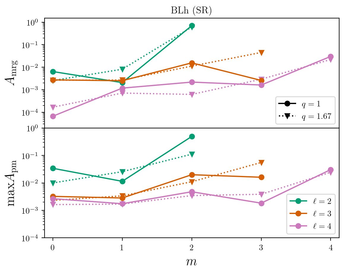
Figure 10: Amplitude at merger and maximum postmerger amplitude of different modes of the GW strain computed with BLh EOS. The upper panel shows the equal-mass binary, while the lower one is a $q=1.67$ case. For unequal-mass coalescences, odd-parity higher-order modes are boosted, e.g. $(2,1)$ and $(3,3)$ modes.

In the context of high mass ratio binary coalescences, higher-order modes could play an important role. The GW strain $h(t,\mathbf{x})$ is the sum of the contribution of the several modes $h_{\ell m}(t,r)$ times the spin-weighted spherical harmonics ${}^{(s)}Y_{\ell m}(\theta,\phi)$ with $s=-2$ that contain the dependence on the source’s sky position,

$$h(t,\mathbf{x})=h_{+}-{\rm i}h_{\times}=\sum_{\ell,m}h_{\ell m}(t,r)\,{}^{(-2)}Y_{\ell m}(\theta,\phi)\ .$$ (9)

The maximum amplitudes $A_{\ell m}=|h_{\ell m}|$ for the different modes at merger and postmerger are shown in Fig. 10. In equal-mass postmerger waveform $m=1$ are suppressed at merger (top panel, solid lines), and the dominant modes are, in order, $(\ell,m)=(2,2),(3,2)$ and $(4,4)$. The contribution of the odd modes and $(2,0)$ increases in the postmerger. The $(2,0)$ mode, in particular, is relevant in the early postmerger times and its amplitude could reach the 15% of the $(2,2)$ amplitude. This is sometimes interpreted as due to radial oscillations of the remnant which contribute to the emitted signal and could generate a coupling with the dominant mode Stergioulas et al. (2011) in analogy to what happens with nonlinear perturbations of equilibrium NS Dimmelmeier et al. (2006); Passamonti et al. (2007); Baiotti et al. (2009); Stergioulas et al. (2011). The waveform mode hierarchy for high-$q$ binaries is similar to that of the $q=1$ binaries. However, the odd modes have a larger relative contribution to the signal during the late inspiral at merger (Cf. Dietrich et al. 2017). The amplitudes of these modes can be up to the 20% of the $(2,2)$ amplitude before merger and in the late postmerger. However, inspection of the waveforms show that during the very dynamical early postmerger phase the amplitude of the $(2,1)$ and $(3,3)$ modes can instantanously reach the same order of the $(2,2)$. The contributions of the subdominant modes in the GW correlates to density modes in the NS remnant triggered in asymmetric mergers, see e.g. Stergioulas et al. (2011); Bernuzzi et al. (2014).

6 Dynamical ejecta

Table 4: Dynamical ejecta average properties for each simulation and for different resolutions. $M_{\text{ej}}$ is the total mass of the ejecta; $\langle\theta_{\text{ej}}\rangle$ and $\langle\phi_{\text{ej}}\rangle$ are the mass weighted rms of the polar and azimuthal angle, respectively; $\langle\upsilon_{\text{ej}}\rangle$ and $\langle Y_{e}\rangle$, are the mass-averaged electron fraction and speed. The last column is the ratio $X_{s}=M_{\rm ej}^{\rm shocked}/M_{\rm ej}$, where the shocked and tidal ejecta are defined by those with entrpy respectively above and below the threshold of $10k_{B}$ per baryon. Simulations without turbulent viscosity are indicated with *.

EOS	$q$	Grid	$M_{\text{ej}}$	$\langle\theta_{\text{ej}}\rangle$	$\langle\phi_{\text{ej}}\rangle$	$\langle\upsilon_{\text{ej}}\rangle$	$\langle Y_{e}\rangle$	$X_{s}$
			$[10^{-2}M_{\odot}]$	$[{}^{\circ}]$	$[{}^{\circ}]$	$[c]$
BLh	1.0	SR	0.136	39	101	0.18	0.263	0.82
BLh	1.0	LR	0.131	40	103	0.16	0.268	0.87
BLh	1.67	HR	0.507	19	58	0.13	0.083	0.21
BLh	1.67	SR	0.451	24	53	0.13	0.114	0.30
BLh	1.67	LR	0.386	24	63	0.11	0.106	0.28
BLh	1.8	HR	0.830	6	26	0.11	0.025	0.01
BLh	1.8	SR	0.762	7	29	0.11	0.030	0.02
BLh	1.8	LR	0.841	7	30	0.12	0.043	0.02
BLh*	1.8	HR	1.014	6	26	0.12	0.020	0.00
BLh*	1.8	SR	1.056	6	28	0.12	0.029	0.01
BLh*	1.8	LR	1.142	7	30	0.12	0.035	0.02
LS220	1.0	SR	0.137	38	104	0.16	0.260	0.71
LS220	1.0	LR	0.170	35	106	0.17	0.233	0.64
LS220*	1.0	HR	0.105	37	103	0.16	0.223	0.71
LS220*	1.0	SR	0.171	33	98	0.16	0.217	0.64
LS220*	1.0	LR	0.215	35	105	0.18	0.218	0.59
LS220	1.67	SR	0.842	12	60	0.14	0.060	0.10
LS220	1.67	LR	1.383	14	56	0.15	0.070	0.15
LS220*	1.67	SR	0.859	8	58	0.13	0.033	0.03
LS220*	1.67	LR	1.047	7	65	0.13	0.050	0.04
SFHo	1.0	HR	0.354	31	106	0.20	0.211	0.69
SFHo	1.0	SR	0.451	34	106	0.19	0.208	0.72
SFHo	1.0	LR	0.698	36	73	0.11	0.332	0.90
SFHo	1.67	SR	0.140	12	52	0.12	0.069	0.13
SFHo	1.67	LR	0.146	10	56	0.13	0.071	0.08
SLy4	1.0	SR	0.072	33	94	0.25	0.240	0.84
SLy4	1.0	LR	0.102	29	103	0.28	0.210	0.66
SLy4	1.67	SR	0.310	7	41	0.12	0.047	0.03
SLy4	1.67	LR	0.305	10	52	0.13	0.067	0.08
SLy4	1.8	SR	0.729	6	40	0.13	0.047	0.01
SLy4	1.8	LR	0.595	7	35	0.13	0.053	0.03

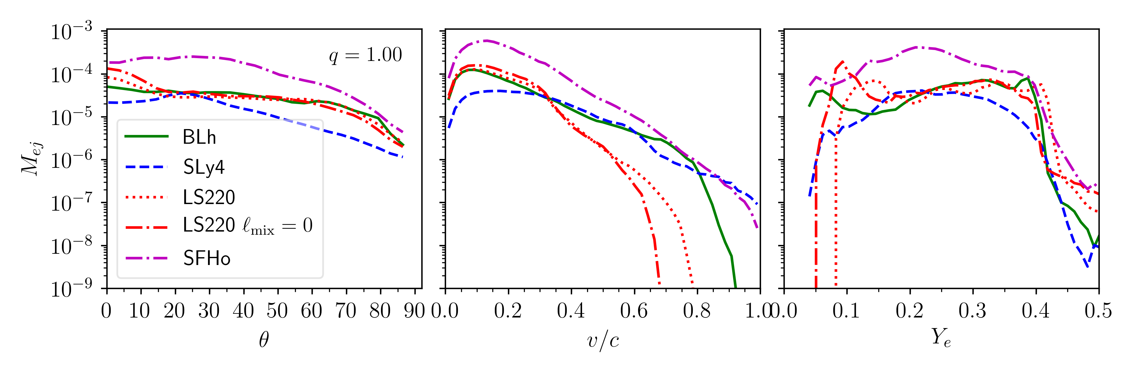
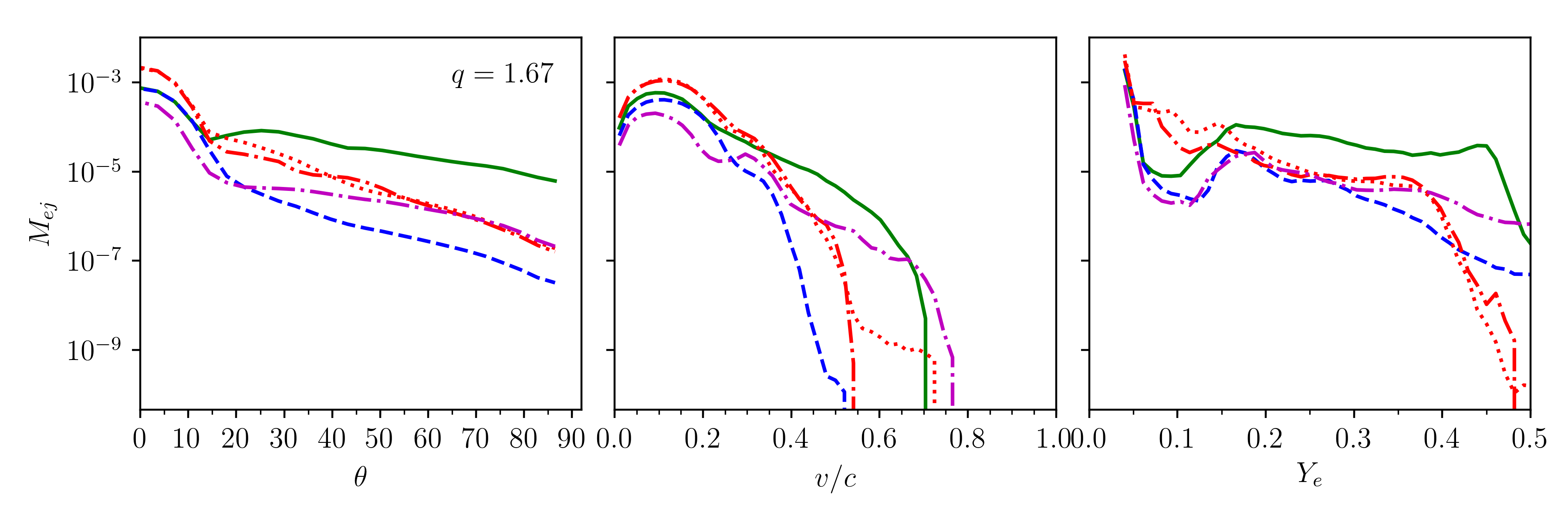
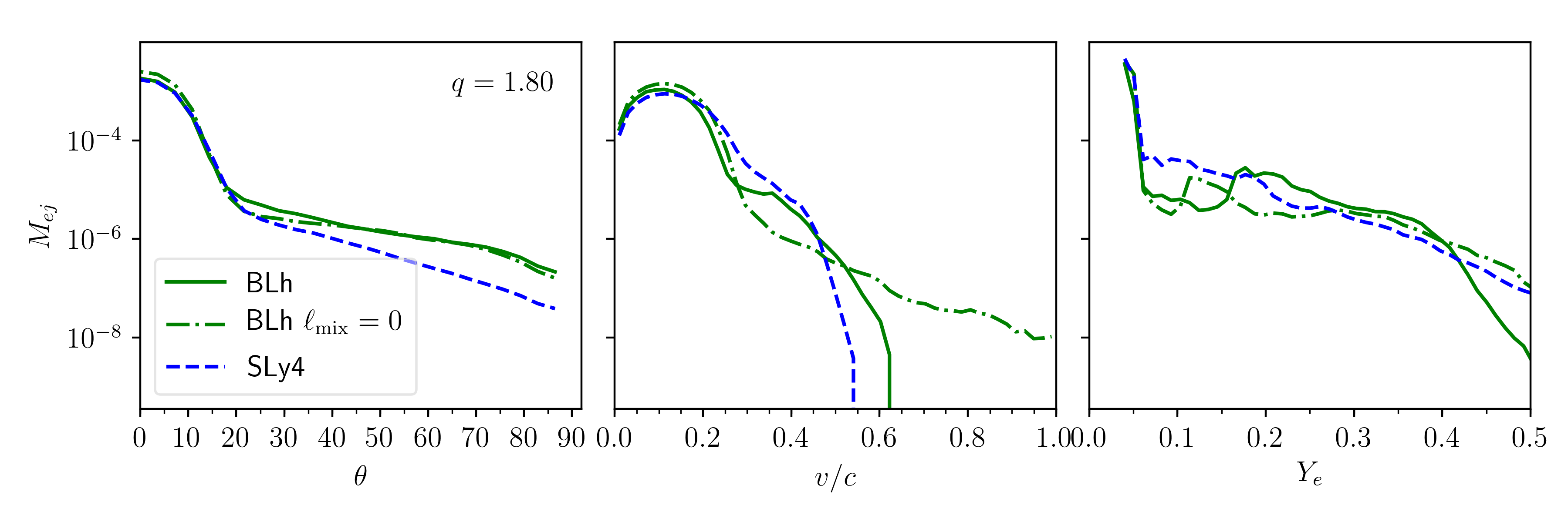
Figure 11: Distributions of the ejecta mass in the polar angle (left), velocity (middle) and electron fraction (right) of the dynamical ejecta. Each row refers to a different mass ratio, from top to bottom $q=1,1.67,1.8$. Note that the angle $\theta=0^{\circ}$ identifies the orbital plane, while $\theta=90^{\circ}$ is the pole above the remnant. Data refer to resolution SR; data from simulations without turbulent viscosity are also shown.

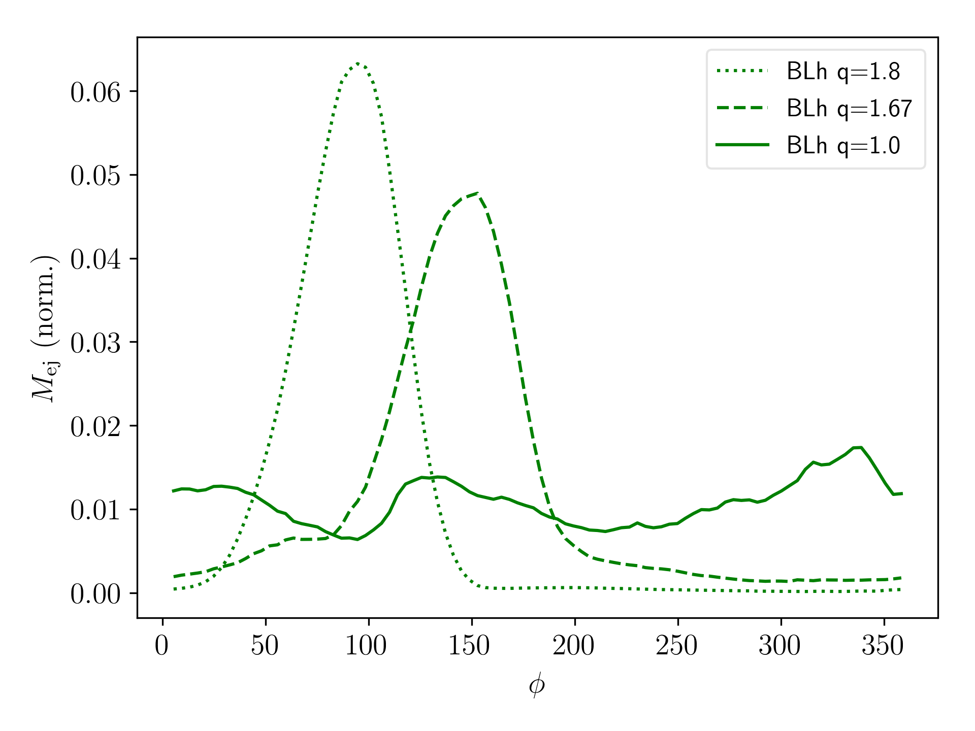
Figure 12: Distribution of the cumulative dynamical mass ejecta in the azimuthal angle for the BLh BNS. The ejecta of the high-$q$ binaries expands with a crescent-like geometry similar to what found in simulations of black-hole–neutron-star binaries. The mass is normalized to the total ejecta mass.

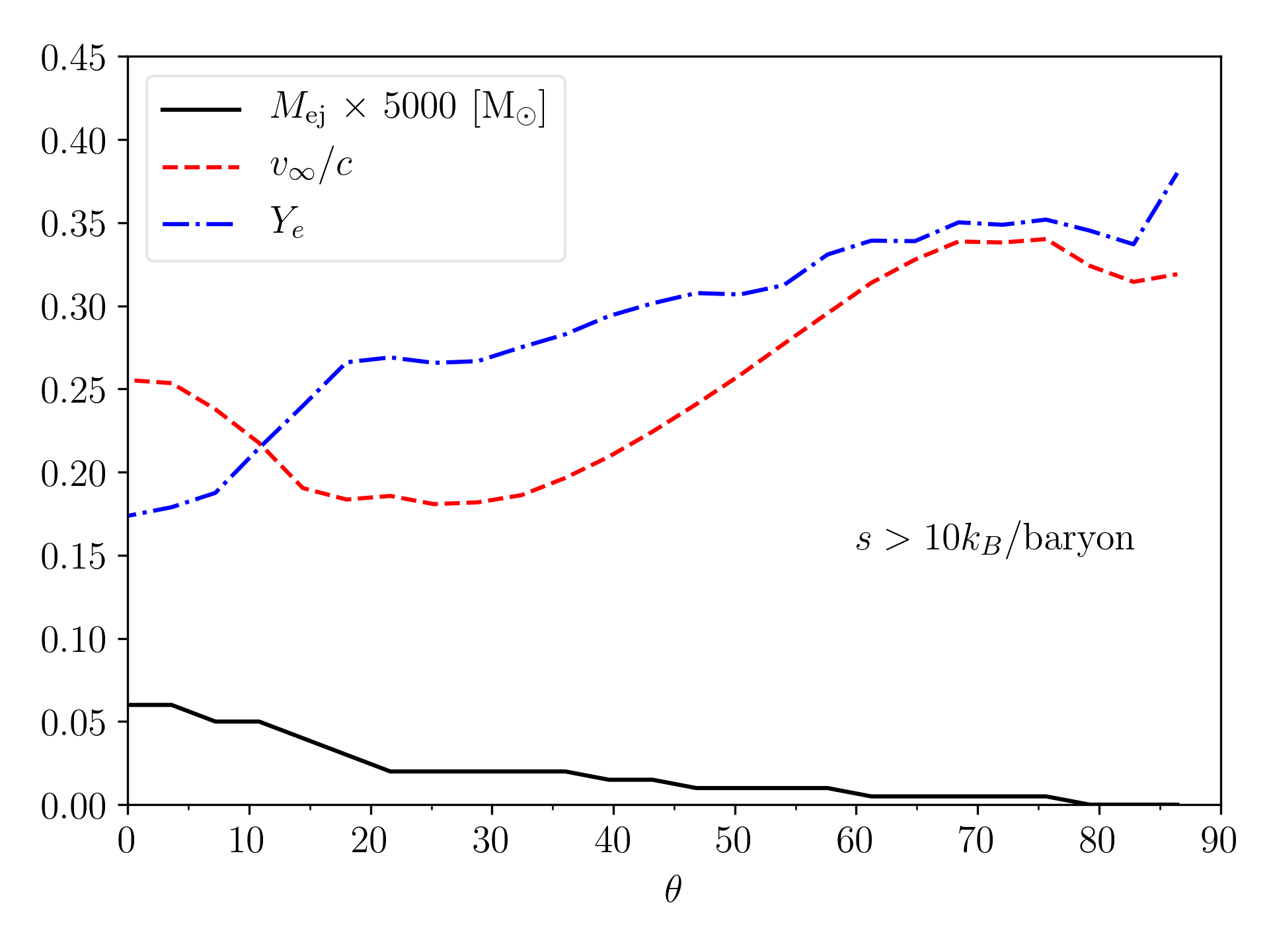
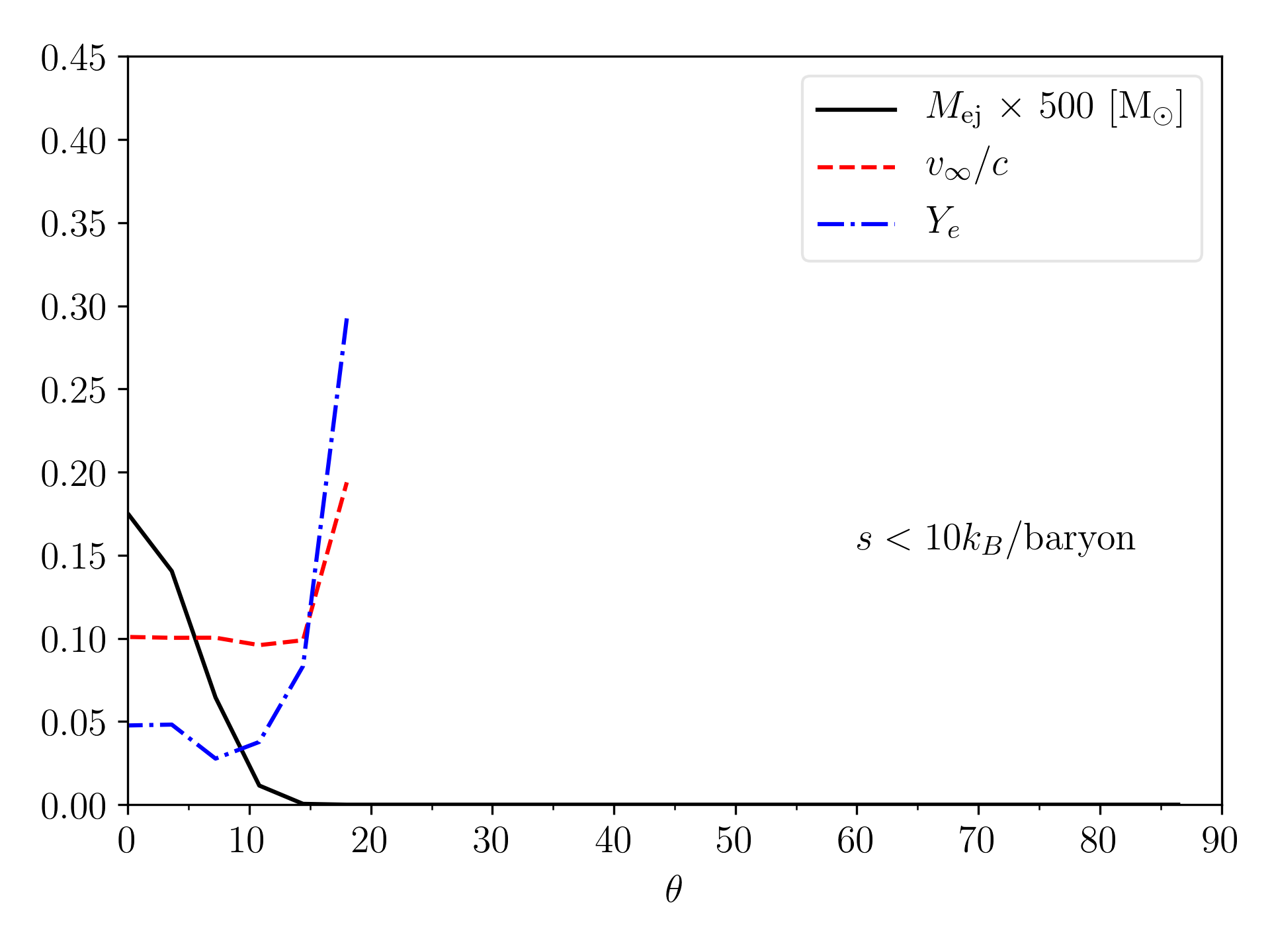
Figure 13: Dynamical ejecta cumulative profiles of shocked (left) and tidal (right) components for BLh $q=1.67$ (SR) as a function of the polar angle. The different lines are the mass, the velocity and the electron fraction. Tidal and shocked components are conventionally separated by flagging fluid elements with specific entropy smaller or larger than $10k_{B}$ per baryon, respectively. Note that the angle $\theta=0^{\circ}$ identifies the orbital plane, while $\theta=90^{\circ}$ is the pole.

Mass ejecta are calculated on coordinate spheres at $r\simeq 300$ km assuming stationary spacetime and flow, and flagging the unbound mass according to the geodesic criterion. A particle on geodesics is unbound if the 4-velocity component $u_{t}\leq-1$ and thus it reaches infinity with velocity $v_{\infty}\simeq(1-u^{2}_{t})^{1/2}$. This geodesic criterion neglects the fluid’s pressure, thus potentially underestimating the mass, but it is considered appropriate for the dynamical ejecta that are moving on ballistic trajectories, e.g. Kastaun & Galeazzi (2015).

We compute the mass-histograms of the ejecta main properties and show them in Fig. 11. In the case of equal mass BNS (top panels), dynamical ejecta are distributed all over the solid angle and composed of both the tidal and the shocked component, (e.g., Hotokezaka et al. 2013; Bauswein et al. 2013b; Sekiguchi et al. 2015; Radice et al. 2018d). The velocity of the material peaks at $v\sim 0.1-0.2$ c and has high speed tails extending up to $v\sim 0.6-0.8$ c. The largest tail velocities are reached by the softest EOS and in the polar regions, where baryon pollution is minimal, as a consequence of the NS cores’ bounce (Fig. 3 of Radice et al. 2018d). Note however, masses ejecta ${\ll}10^{-5}$ and velocities ${\gtrsim}0.9$ c cannot be trusted and can suffer of large numerical errors due to the atmosphere treatment and imperfect mass conservation (Appendix B). The ejecta’s composition is characterized by a wide range of $Y_{e}$; for the LS220 and the BLh EOS two peaks at ${\sim}0.1-0.15$ and at ${\sim}0.4$ are clearly visible; they roughly correspond to the shocked and tidal components, although the former has also a significant amount of material with low $Y_{e}$ material. Note the SFHo model peaks instead at ${\sim}0.25$. Comparing the two equal mass LS220 BNS, we find a small effects of turbulent viscosity: the viscous ejecta have a more prominent peak at lower $Y_{e}$ and a slightly reduced tidal component, possibly due to the difference in the early-postmerger dynamics around the moment of core bounce.

The dynamical ejecta of asymmetric BNS with $q\gtrsim 1.67$ (middle panels of Fig. 11) are quantitatively different from symmetric BNS. The ejected material is distributed more narrowly about the orbital plane and decreases almost monotonically to the polar latitudes. The dependence on the azimuthal angle is also very different from the equal-mass cases. Because the matter is almost entirely expelled by tidal torques, the ejecta is distributed over a fraction of the azimuthal angle around its ejection angle and has a crescent shape, Fig. 12. This is similar to what observed in black-hole–neutron-star binaries Kyutoku et al. (2015); Kawaguchi et al. (2016). Hence, the ejecta for high-$q$ BNS are not formed isotropically. Most of the unbound mass has low $Y_{e}\lesssim 0.1$, although several $q=1.67$ BNS have a second peak at ${\gtrsim}0.4$. Thus, while the tidal component is the dominant for asymmetric BNS, a small shocked component persists. The velocity distributions have comparable peak values indicating that the tidal component has velocities comparable to those of shocked component (Cf. Fig. 6 of Dietrich et al. 2017). Note that the fast tails are suppressed for increasing mass ratio. This is because of the less violent merger and bounce experienced by these binaries. These features are even more extreme for the $q=1.8$ case (bottom panels of Fig. 11). The above results appear consistent with those reported in Sekiguchi et al. (2015); Lehner et al. (2016), although different EOS and more moderate mass ratio were used there.

The mass-averaged properties of the dynamical ejecta computed from the histograms are reported in Tab. 4. We show results for all the resolutions available in order to convey an idea of the uncertainties. The latter are difficult to precisely quantify since strict convergence is not observed in the data. However, the results are robust for a large variation of the grid resolution with mass variations at the ${\sim}20\%$ level between SR and HR and less than a factor two between LR and SR. Note there is a factor 2 (1.5) between the spacing of LR and SR (SR and HR) grids. The following discussion mostly refers to highest resolutions available, as the LR is not always sufficient to properly resolve the composition (see below).

The large mass asymmetry can boost the mass ejecta by up to a factor four with respect to the equal mass cases. The average electron fraction of the dynamical ejecta from asymmetric BNS is ${\sim}0.11$, a factor two smaller than for the respective equal mass BNS. The mass-distribution is concentrated around the equatorial plane. The rms of the polar angle is ${\sim}5-15^{\circ}$ for asymmetric BNS with $q=1.8-1.67$, while it is ${\sim}35^{\circ}$ for symmetric BNS. Overall these results show that while the tidal component of the dynamical ejecta is dominant with respect to the shocked ejecta in high mass ratio binaries, a delayed collapse can produce unbound mass with electron fractions that can extend to $Y_{e}\sim 0.4$. The rms of the azimuthal angle is reduced from ${\lesssim}106^{\circ}$ of symmetric BNS to less than half, ${\gtrsim}50^{\circ}$, for asymmetric BNS. We recall that the rms of a uniform distribution with support on the segment $2\alpha\in(0,2\pi]$ is $\langle\phi\rangle=\sqrt{3}/3(\pi-\alpha)$, thus giving $\langle\phi\rangle\simeq 104^{\circ}$ if the support is the full interval ($360^{\circ}$) and $\langle\phi\rangle\simeq 54^{\circ}$ if the support is half of the interval ($180^{\circ}$). A similar argument holds also for the polar angle support around the equator, $\pi/2-\alpha\leq\theta\leq\pi/2+\alpha$, for which $\langle\theta\rangle=\left(\sqrt{3}/3\right)\alpha$. This is correct as far as the ejecta is emitted uniformly over a small portion around the equator (a good approximation in the case of high mass ratio BNS).

The tidal and shocked contributions to the dynamical ejecta are calculated by conventionally distinguishing the unbound matter with specific entropy smaller or larger than $10k_{B}$ per baryon, respectively  Radice et al. (2018d). The last column of Tab. 4 reports the ratio

$$X_{s}=\frac{M_{\rm ej}^{\rm shocked}}{M_{\rm ej}}=\frac{M_{\rm ej}^{\rm shocked}}{M_{\rm ej}^{\text{tidal}}+M_{\rm ej}^{\rm shocked}}\ ,$$ (10)

indicating the mass fraction of the shocked ejecta to the total value. For the BLh EOS $X_{s}$ increases from $0.01$ to $0.3$ and $0.9$ for $q=1.8$ to $1.67$ and $q=1$, respectively. For the SLy EOS $X_{s}\simeq 0.01$ for $q=1.8$ and $q=1.67$ that have a similar dynamics charcaterized by the accretion-induced BH formation and prominent tidal ejecta, and $X_{s}\simeq 0.8$ for $q=1$. The other two $q=1$ mergers with short-lived NS remnants have $X_{s}\simeq 0.7$ that reduces to $0.1$ for $q=1.67$.

As an example, we discuss mass-histograms for the shocked and tidal components separately for the BLh $q=1.67$, Fig. 13. The tidal component is confined within an angle of $\theta\lesssim 10^{\circ}$ from the orbital plane; most of the mass has $Y_{e}\sim 0.05$ with the largest electron fractions $Y_{e}\sim 0.15$ reached at those latitudes. The velocities are uniformly distributed $v\sim 0.1$ c. The shocked component, instead, has mass mostly distributed at angles $\theta\sim 25^{\circ}$ but it extends to polar latitudes. The ejecta has electron fraction $Y_{e}\sim 0.17-0.25$ for $\theta\lesssim 25^{\circ}$ and $Y_{e}\sim 0.30-0.35$ for $\theta>60^{\circ}$. The velocity of the bulk ejecta at the orbital latitudes is $v\lesssim 0.25$ c, minimal at around $\theta\sim 27^{\circ}$, and has a peak $v\lesssim 0.3$ c at polar latitudes. In general, the shocked component is slightly delayed with respect the tidal component because it is generated when the NS cores’ bounce Radice et al. (2018d).

Table 4 also highlights a dependency on resolution, especially for high mass ratios BNS. This is expected since resolving NS with different sizes is more challenging than with equal sizes for the box-in-box AMR. In particular, the LR resolutions does not seem sufficient to deliver quantitatively robust results for all the cases, especially at high $q$ and with viscosity. Note, for example, that ejecta mass decreases with resolutions indicating numerical dissipation plays a role enhancing the ejecta. Moreover, $Y_{e}$ raises very rapidly from the NS surface; in the case the latter is not well resolved the tidal ejecta might be spuriously composed of material from the interior, as observed in the BLh $q=1.8$ LR simulation.

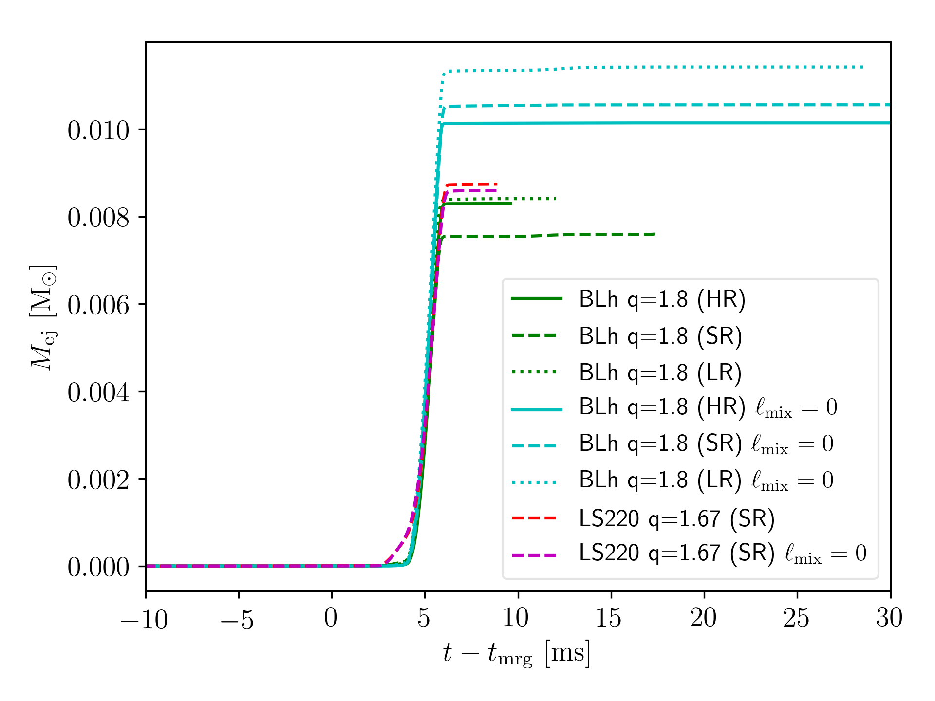
Figure 14: Dynamical mass ejecta in viscous and nonviscous simulations. The viscous dynamical ejecta reported in Radice et al. (2018c) is here not present because the shocked component ejecta is negligible. Furthermore, the angular momentum distribution introduced by the subgrid model $\ell_{\rm mix}(\rho)$ appears to be dependent on the EOS model. Note the turbulent viscosity subgrid model employed here is different from the $\ell_{\rm mix}$ employed in previous simulations.

We finally comment on the effect of viscosity on the dynamical ejecta. Radice et al. (2018c) pointed out that the dynamical ejecta in asymmetric BNS can be enhanced by the thermalization of mass accretion streams between the secondary and the primary neutron star. This viscous component of the dynamical ejecta are characterized by large asymptotic velocities and have masses that depend on the efficiency of the viscous mechanism. Figure 14 shows the ejecta mass for the BLh $q=1.8$ and LS220 $q=1.67$ BNS. The viscous dynamical ejecta is not present because the shocked component ejecta is negligible. Actually, the turbulent viscosity here can reduce the tidal dynamical ejecta as a consequence of the different angular momentum distribution due to turbulence. Note the effect is significant and robust with respect to the variation of the grid resolution. The effect of viscosity is much reduced in the LS220 $q=1.67$ BNS and practically negligible considering the numerical uncertainties (only the SR is shown for clarity). This might be related to the differences in the EOS at low density (Sec. 2). The simulations of Radice et al. (2018c) employed the GRLES scheme as those presented here, but using $\ell_{\text{mix}}=const$ and varying systematically the constant for the turbulent parameter. We cannot currently exclude that the specific subgrid model $\ell_{\text{mix}}(\rho)$ built from Kiuchi et al. (2018) determines a different effect with respect to the $\ell_{\text{mix}}=const$ model. A detail investigation of the viscous dynamical ejecta with the subgrid model $\ell_{\text{mix}}(\rho)$ for intermediate values of $q$ will be presented elsewhere.

7 Synthetic kilonova light curves

We compute synthetic kilonova light curves for each of the BNS mergers presented in this work. We use a semi-analytical multicomponent, anisotropic kilonova model that takes into account the angular distribution of the ejecta properties as well as the presence of different kinds of ejecta Perego et al. (2017); Radice et al. (2018a); Radice et al. (2018d); Barbieri et al. (2020). The latter differ by the mechanisms that cause the ejection and the timescales over which they operate. Within this framework, the homologously expanding ejecta is discretized in velocity space and the photon diffusion time is estimated by timescale arguments. Radiation is assumed to be in local thermodynamical equilibrium up to the relevant photosphere and photon emission is modelled as a superposition of blackbody spectra. The different ejecta components comprise the dynamical ejecta discussed in Sec. 6 and possibly winds expelled by the remnant disc on longer timescales (0.1-1s) by means of neutrino irradiations and turbulent viscosity of magnetic origin. The kilonova emission produced by each component depends mainly on three quantities that characterize the ejecta, namely the amount of mass, $M_{\rm ej}$, its average expansion velocity, $\langle v_{\rm ej}\rangle$, and an (effective) grey photon opacity, $\kappa_{\rm ej}$. In all our kilonova models, we locate the merging BNS at a distance of 40 Mpc and we consider a reference viewing angle of $\pi/6$ with respect to the rotational axis of the binary. If not otherwise specified, the model parameters and input physics are assumed to be as in the best fit model named ${\rm BF}$ to AT2017gfo of Perego et al. (2017).

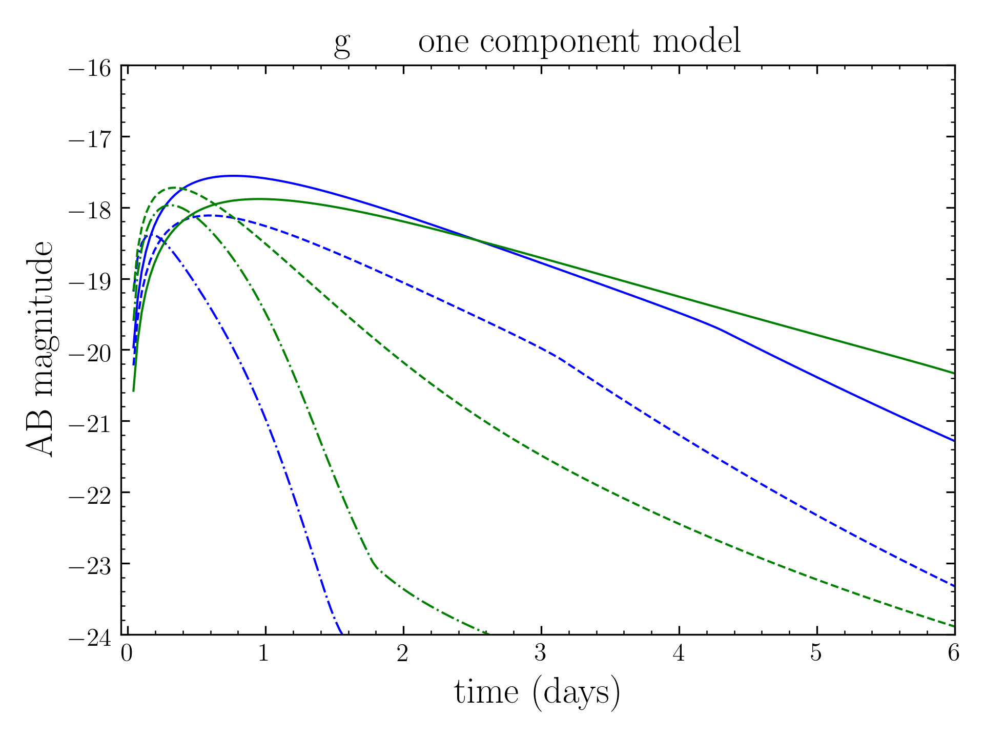
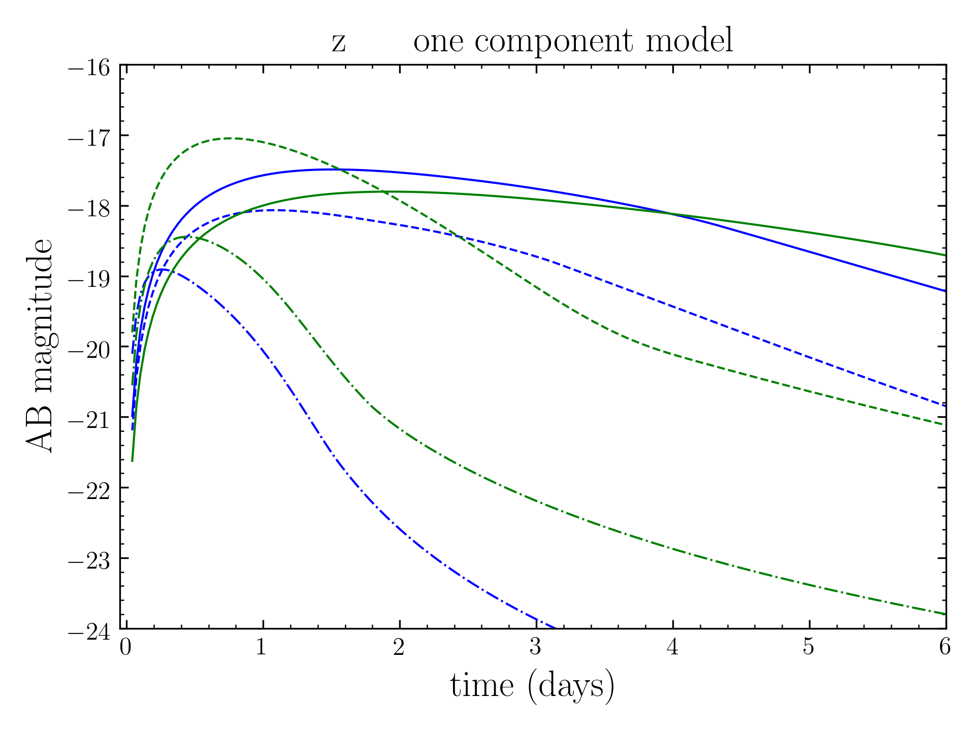
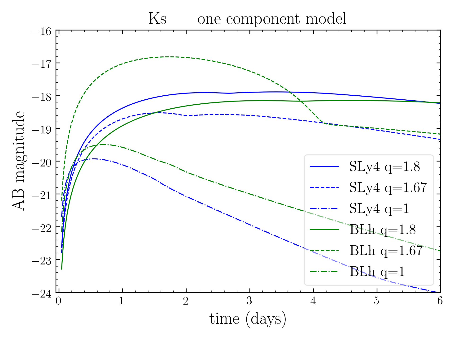
Figure 15: Kilonova light curves from the simulated dynamical ejecta (one component) for the BLh and SLy BNS. The ejecta properties are taken from the simulation at the highest grid resolution. The light curves are computed with the axisymmetric models of Perego et al. (2017) for $q=1$ and of Barbieri et al. (2020) for $q=1.67,1.8$. Binaries are always assumed to be located at a distance of 40 Mpc and to be observed under a viewing angle of $30^{\circ}$ with respect to the BNS rotational axis. The bump observed in the $K_{s}$ band for the BLh $q=1.67$ model results from the radial emission from the crescent pointing towards the observer.

We first examine the kilonova emission obtained by considering only the dynamical ejecta discussed in Sec. 6. In the case of $q=1$ mergers, matter is expelled over the entire solid angle and we follow the model presented in Perego et al. (2017); Radice et al. (2018a); Radice et al. (2018d). We assume the ejecta to be axisymmetric and the photon diffusion to proceed mostly radially. In these cases, we discretize the polar angle in 30 slices over the whole solid angle. We use azimuthal averages of the angular distribution of the ejected mass, electron fraction and of mean expansion velocity directly extracted from the latest stages of our NR simulations. While the ejecta mass and mean velocity are directly input into the kilonova model, the electron fraction is used to assign the ejecta opacity according to $\kappa_{\rm dyn}=1~{}{\rm cm^{2}~{}g^{-1}}$ for $\langle Y_{e}\rangle>0.25$, $\kappa_{\rm dyn}=20~{}{\rm cm^{2}~{}g^{-1}}$ otherwise (Cf. Kasen et al. (2013); Tanaka et al. (2019); Fontes et al. (2020).) Alternatively, for the $q=1.67$ and $q=1.8$ cases the dynamical ejecta is confined (in very good approximation) within a crescent across the equatorial plane (see Sec. 6) and we emply the model described in Barbieri et al. (2020) (see also Kawaguchi et al. 2016) in which the photon emission is the combination of radial and lateral emissions from an optically thick disc. In this case, we use the total ejecta mass, $M_{\rm ej}$, and mean velocity, $\langle v_{\rm ej}\rangle$, obtained by our NR simulations to initialize a vertically homogeneous, radially expanding disc. For the grey opacity, we assume always $\kappa_{\rm dyn}=20{\rm cm^{2}~{}g^{-1}}$ since in these cases $\langle Y_{e}\rangle<0.25$ (often $\langle Y_{e}\rangle<0.10$). For the disc half-opening angle in the polar direction we use $\theta_{\rm disc}=\sqrt{3}\langle\theta_{\rm ej}\rangle$, while for the azimuthal disc opening we set $\phi_{\rm disc}=2\sqrt{3}\langle\phi_{\rm ej}\rangle$ (See Sec. 6). The crescent shape breaks the axisymmetry of the emission. In our calculations, we always assume the dynamical ejecta to be emitted toward the observer. For small polar opening angles, this assumption is not very relevant, since the radial emission is subdominant. In the case of larger discs (as in the BLh $q=1.67$ case) the radial emission can be relevant and our model assumptions can be more questionable.

In Fig. 15, we present light curves in three different photometric bands ($g$, $z$, and $K_{s}$) to span the relevant wavelength interval from visible to near-infrared radiation, for the three different models obtained with the BLh and SLy4 EOS. We first notice that, even in the case of prompt collapse, BNS mergers can power bright kilonovae Kawaguchi et al. (2020); Kyutoku et al. (2020). In particular, in the high-$q$ models the light curves from the dynamical ejecta are possibly brighter, with wider light curves peaking at later times compared with the $q=1$ mergers. This is due to the crescent-like configuration of the expanding ejecta (Cf. Tanaka et al. (2014); Korobkin et al. (2020).) On the one hand, when matter is emitted over a large portion of the solid angle (as it usually happens for $q\sim 1$) the hotter ejecta is buried inside the optically thick region and high energy photons have to diffuse and thermalize before being emitted in the kilonova. On the other hand, thanks to the disc-like geometry of the crescent, the innermost, hotter portion of the disc provides a significant contribution to the kilonova emission at any time, explaining the brighter and more substained emission. These effects are visible in all bands, but the increase in magnitude moving from $q=1$ to higher $q$’s is more pronunced in the infrared band as a consequence of the lower electron fraction (and thus of the higher opacity) of the dynamical ejecta in the crescent. This effect is even amplified by the larger amount of dynamical ejecta observed in the high-$q$ models (with the only exception of the SFHo models).

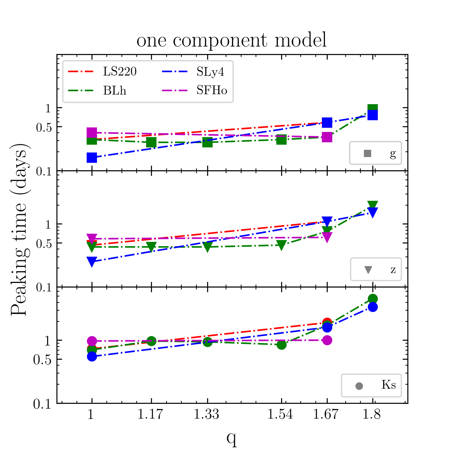
Figure 16: Peak time of the one component kilonova models as a function of the mass ratio for all the simulated BNS. Data from BLh simulations at intermediate mass ratios are also included (See Appendix B). Note the log scale and that straight lines connecting the points are due to the limited number of simulations available and do not represent accurately the functional behaviour in the mass ratio.

The peak times of all kilonova models are shown as a function of the mass ratio in Fig. 16. In addition to the models presented in Tab. 1, we include here also a few more LR models computed with the BLh EOS (See Appendix B) to better explore the dependence on $q$. The kilonova peak times of mergers undergoing accretion-induced prompt collapse are significantly delayed with respect to the $q=1$ cases. For the BLh merger, the emission in $g$, $z$ and $K_{s}$ bands peaks between few hours and within a day respectively if $q=1$, and and between a day and a week if $q=1.8$. The near-infrared frequencies are those that vary most as a function of the mass ratio. The SLy4 light curves shows a similarly behaviour, although less data points are available. Less variation in the peak times is observed in the LS220 and SFHo mergers between $q=1$ and $q=1.67$, but note that in those cases the dynamical ejecta mass also vary less with the mass ratio.

We tested that the features described above do not depend on the specific velocity profile for the homologously expanding ejecta, in which most of the mass resides in the innermost part of the disc. Indeed, a flat distribution in the expanding velocity as employed in Kawaguchi et al. (2016), provides very similar results. This is due to a compensation effect between the larger amount of decaying material and the denser (thus, optically thicker) vertical profile of the disc in our models. These features are robust also with respect to the uncertainties on the ejecta properties of numerical origin. Considering the ejecta properties extracted from simulations at different resolutions gives some quantitative changes that mostly affect the light curves’ luminosity. Here is worth to remark that a factor two of uncertainty in the ejecta mass can translate in up to an order of magnitudes in luminosity. Moreover, current light curve models suffer of larger systematic uncertainties in nuclear (e.g. mass models, fission fragments and $\beta$-decay rates) and atomic (e.g. detailed wavelength dependent opacities for $r$-process element) physics (Eichler et al., 2015; Rosswog et al., 2017; Gaigalas et al., 2019).

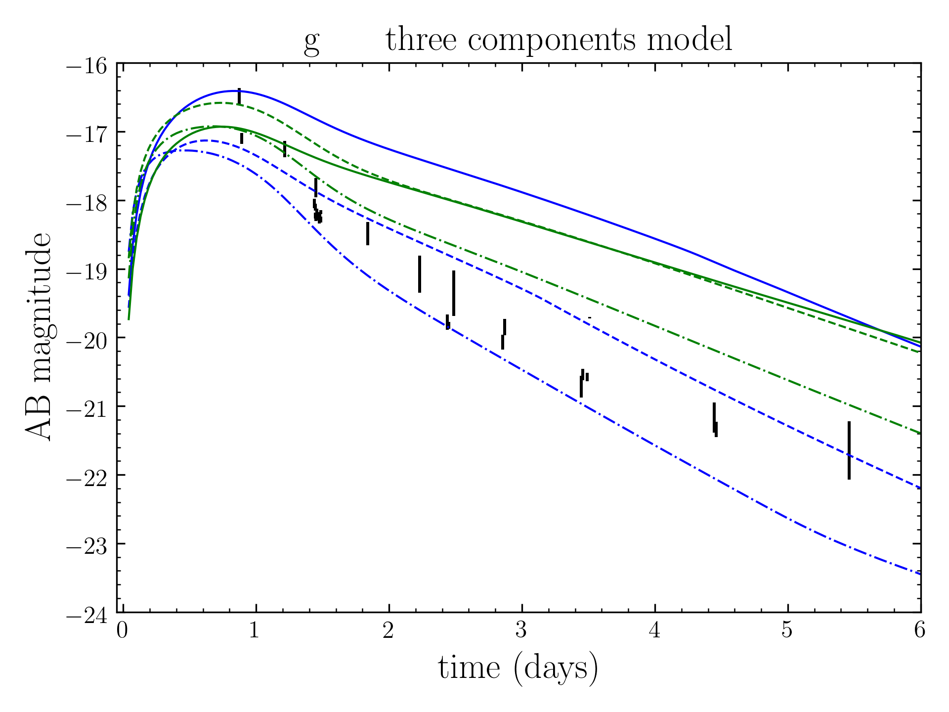
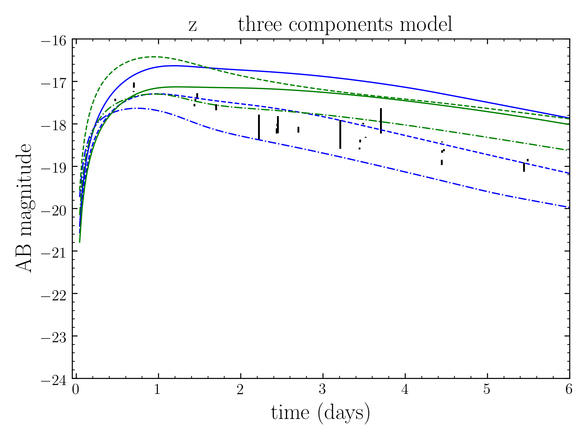
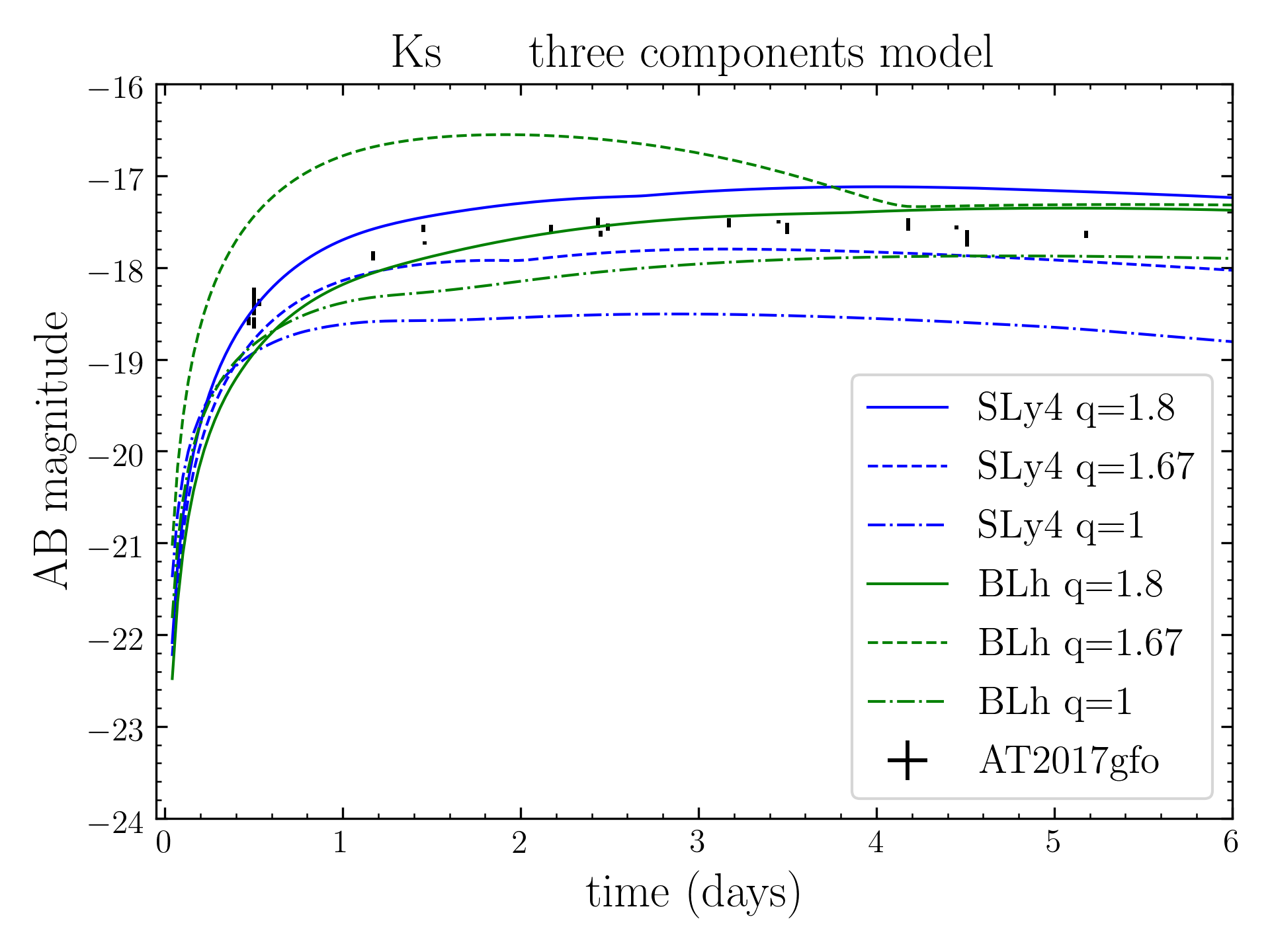
Figure 17: Kilonova light curves as in Fig. 15, but employing a three component model for the BLh and SLy BNS. The dynamical ejecta component is taken as in Fig. 15. The other two components are assumed from a neutrino-driven and a viscosity-driven wind. The neutrino-wind mass is assumed 5% (1%) of the disc mass if the remnant is a long-lived (short-lived or promptly collapsing) massive NS; the effective grey photon opacity is set $\kappa_{\rm w}=1~{}{\rm cm^{2}~{}g^{-1}}$, while the wind expands within a $\pi/4$ angle around the polar axis with an average speed of $\langle v_{\rm w}\rangle=0.08c$. The viscos-wind mass is assumed 20% of the disc mass, expanding with an average speed of $\langle v_{\rm v}\rangle=0.06c$, and with a grey opacity is set to $\kappa_{v}=5~{}{\rm cm^{2}~{}g^{-1}}$. The observational data of AT2017gfo are shown as black markers for comparison (see discussion in text).

The models presented in Fig. 15 do not contain potentially relevant contributions to the total ejecta coming from disc winds. Thus, the resulting light curves could be considered as lower limits for the kilonova emission. To estimate the potential impact of the disc wind emission on our results, in Fig. 17 we also present light curves obtained by considering a three component kilonova model for the same three photometric filters and models of Fig. 15. The dynamical ejecta profiles are NR informed as previously discussed. For the disc winds, we consider both a neutrino-driven and a viscosity-driven wind. Since wind ejection is expected over a wide portion of the solid angle, we model the related kilonova emission using again the framework described in Perego et al. (2017); Radice et al. (2018a); Radice et al. (2018d). For the neutrino-driven wind component, the amount of ejecta is assumed to be 5% (1%) of the disc mass if the remnant is a long-lived (short-lived or promptly collapsing) massive NS. Due to the effects of neutrino irradiation, the effective grey photon opacity is set $\kappa_{\rm w}=1~{}{\rm cm^{2}~{}g^{-1}}$, while the wind expands within a $\pi/4$ angle around the polar axis with an average speed of $\langle v_{\rm w}\rangle=0.08c$. For the viscous wind component, the amount of ejecta is always assumed to be 20% of the disc mass, expanding with an average speed of $\langle v_{\rm v}\rangle=0.06c$, while the grey opacity is set to $\kappa_{v}=5~{}{\rm cm^{2}~{}g^{-1}}$. To compute the masses of the wind ejecta we consider the disc masses presented in Sec. 4.

Since the disc ejecta is usually more relevant than the dynamical one (see, e.g., Radice et al. 2018d), the large differences between $q=1$ and high-$q$ models in the kilonova light curves observed in the one component models reduce for the multi-component cases. Nevertheless, since BNS mergers with higher mass ratios tend to produce also more massive discs, also these possibly more complete models confirm that BNS mergers undergoing prompt merger can power bright kilonovae and high-$q$’s can possibly produce kilonovae that are brighter and charaterized by wider peaks in all relevant bands, compared to more symmetric mergers mergers that have the same chirp mass. More specifically, in the case of high-$q$ binary models for which the dynamical ejecta has a relatively large mass (up to $10^{-2}M_{\odot}$) and is highly anisotropic (e.g. BLh and SLy4 $q=1.8$), the emission from the crescent is significant at all time and possibly dominant for mergers forming discs of not too large masses ($M_{\rm disc}\lesssim 0.1M_{\odot}$). The opposite scenario is realized in symmetric binaries: in all $q=1$ models, irrespectively of the EOS, the low mass, widely distributed dynamical ejecta has a visible impact on the light curves only at very early times and in the blue portion of the kilonova spectrum. At later times, and especially at red and infra-red frequencies, the emission is dominated by disc winds.

The observations of AT2017gfo (Villar et al. 2017 and refs20200807 therein) are also included in Fig. 17 and can be qualitatively compared to the lightcurves from the simulations (note that the simulated BNS have chirp mass consistent with GW170817). The light curves from high-$q$ mergers are generically flatter and more extended in time than those of AT2017gfo. Assuming these particular light-curve models, the observation of AT2017gfo would exclude high-$q$ and stiff EOS with $\tilde{\Lambda}\gtrsim 600$ (long-lived NS remnants) consistently wih the low-spin prior GW analysis Abbott et al. (2019a, b). The plots also highlight that the light curves in different bands favour different mass ratio, thus anticipating systematics (and degeneracies) between the multicomponents light curves and the binary parameters. We finally remark that the kilonova model employed here avoids the solution of the challenging radiative transfer problem in multi-dimension (e.g. Wollaeger et al., 2018; Kawaguchi et al., 2020; Bulla, 2019) and approximates the time- and frequency-dependent $r$-process opacities with constant, gray opacities. This procedure likely introduces systematic uncertainties that are not easy to quantify. Direct comparisons between simplier analytical models and the outcome of radiative transfer calculations indicate that the former tend to predict lower luminosities and later peaks, especially for $\kappa\gtrsim 100~{}{\rm cm^{2}~{}g^{-1}}$ (Wollaeger et al., 2018). The usage of input parameters gauged on AT2017gfo and of opacities $\lesssim 25~{}{\rm cm^{2}~{}g^{-1}}$ possibly limits these uncertainties. We conservatively estimate a residual uncertainty of $\pm 0.5$ magnitude at peak. Even including these uncertainties, the qualitative differences between AT2017gfo and the light curves obtained for high-$q$ and stiff EOSs still hold.

8 Conclusions

In this paper, we explored in a systematic way the dynamics, the ejecta, and the expected kilonova light curves of highly asymmetric BNS mergers by means of detailed simulations in NR. The latter employed different finite-temperature, composition dependent EOS, and numerical resolutions. The prompt collapse dynamics discussed here for high-$q$ BNS has a underlying mechanisms different from the equal-masses prompt collapse: in the former case, the collapse is driven by the accretion of the companion onto the massive primary star. For binaries with increasing mass ratio and fixed chirp mass, the companion NS undergoes a progressively more significant tidal disruption. Thus, in these BNS sequences accretion-induced prompt collapse should be always present after a critical mass ratio in connection to the maximum NS mass. For example, for the BLh EOS the critical mass ratio should fall in the interval $1.54<q_{\text{thr}}<1.67$.

The remnan BH in these high-mass-ratio mergers is surrounded by a massive accretion disc in contrast to comparable masses prompt collapse merger that have no significant disc left outside the BH. The accretion discs of high-mass ratio mergers are primarily constituted of tidally ejected material, hence they are initially cold and neutron rich. The simulations show that fallback of the tidal tail perturbs the disc and affect its accretion. The long-term disc and fall back dynamics is relevant to understand the complete kilonova emission and also for GRB afterglow (extended) emission Rosswog (2007); Metzger et al. (2010); Desai et al. (2019). This study is left for the future.

Perhaps the most relevant astrophysical consequence of our work is the possibility of having massive dynamical ejecta from these accretion-induced prompt collapsing remnant. The ejecta mass can reach $M_{\text{ej}}\sim 0.007-0.01M_{\odot}$ and are mostly emitted within $10^{\circ}-20^{\circ}$ about the orbital plane and in a portion of $100^{\circ}-180^{\circ}$ in the azimuthal angle. The ejecta are neutron rich with $Y_{e}\lesssim 0.1$ and with velocities $v\lesssim 0.1$ c. The related kilonova light curves are predicted to be usually significantly brighter than the equal masses case (at fixed chirp mas) in all the bands as a consequence of the crescent-like geometry of the expanding dynamical ejecta. The light curves peak at later times and are powered by the sustained emission of the innermost, hotter portion of the crescent especially in the infrared bands.

We suggest that the confident detection (or confident nondetection) of an electromagnetic counterpart for a high-mass binary can directly inform us about the binary mass ratio. Because the latter is currently poorly constrained by GW analysis, the kilonova counterpart can deliver significant complementary information. Multimessenger analysis of high-mass events are thus particularly relevant. They will require a precise numerical relativity characterization of the ejecta in terms of the binary parameters that is not currently available, as well as improved nuclear and atomic physics input or suitably parametrized models for the light curves.

Our results can help interpreting GW190425 in the scenario that the GW was produced by an asymmetric binary with $q\gtrsim 1.6$ (Note the chirp mass for GW190425 is even larger than the one simulated here, while large mass ratios are excluded for GW170817 if spins are small). Using the methods developed in Agathos et al. (2020), Abbott et al. (2020) estimated that the probability for the remnant to prompt collapsed to BH is ${\sim}97\%$. The NR fitting models used in Agathos et al. (2020) refer to equal masses and thus are to be considered conservative for $q\gtrsim 1.6$. Hence, if GW190425 is interpreted as a such asymmetric BNS merger, the BH remnant scenario is further strengthened by our results. Moreover, a bright and temporally extended red kilonova could have been expected as a counterpart if GW190425 was produced by a high-$q$ merger [Cf. Foley et al. (2020)]. The kilonova signal in this case could be similar to the one produced in BH-NS binaries Radice et al. (2018a); Kyutoku et al. (2020).

All of our GW waveforms and ejecta data will be publicly available as part of the CoRe database at

http://www.computational-relativity.org/

Appendix A Experimental estimate of the remnant BH

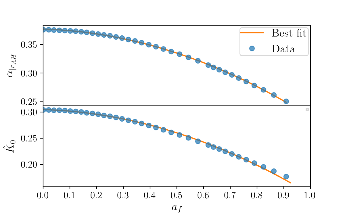
Figure 18: Dependence on the final black hole dimensionless spin of the lapse calculated at the apparent horizon (top) and the extrinsic curvature multiplied by $M_{\rm ADM}$ at the puncture (bottom) and relative best fits.

We perform single puncture experiments with the gauge conditions used in the BNS simulations, and study the behaviour of the lapse $\alpha$ and the extrinsic curvature trace $K$ close to the puncture. We show that the evaluation of the extrinsic curvature $K$ at the puncture (origin) allows us to estimate the BH spin and the lapse at the AH. Further assuming an approximate value for the BH mass as given by the quasiuniversal relation $M_{\text{BH}}\approx M|e_{b}^{\text{mrg}}(\kappa^{T}_{2})|\nu$ (upper bound), leads to a simple estimate of both mass and spin of the BH. Hence, these results could be useful as a simplified criterion for estimating BH formation without a AH.

The gauge conditions for lapse and shift vector $\beta^{i}$ employed in the simulations are Baker et al. (2006); Campanelli et al. (2006); van Meter et al. (2006); Brügmann et al. (2008)

$$\partial_{t}\alpha-\beta^{i}\partial_{i}\alpha =-\alpha^{2}\mu_{L}K$$ (11)

$$\partial_{t}\beta^{i}-\beta^{j}\partial_{j}\beta^{i} =\mu_{S}B^{i}$$ (12)

$$\partial_{t}B^{i}-\beta^{j}\partial_{j}B^{i} =\partial_{t}\tilde{\Gamma}^{i}-\eta B^{i}\ ,$$ (13)

where $\tilde{\Gamma}^{i}$ are the conformal variables of Z4c Bernuzzi & Hilditch (2010); Hilditch et al. (2013), $\eta=1$ is a damping term, $\mu_{S}=3/4$, $\mu_{L}=2/\alpha$ are the characteristic speeds. For simplicity the initial data for one puncture with different spins are prepared solving for two punctures Ansorg et al. (2004) and setting one mass much maller than the other $q\sim 10^{12}$ and at a distance smaller than the evolution grid spacing. These simulations are performed with the BAM code Brügmann et al. (2008) with $6$ refinement levels and maximum resolutions of $h\simeq 4.6875\times 10^{-2},2.34375\times 10^{-2}$. During the evolution the system quickly settles to a stationary solution with mass $M_{\text{BH}}$ and dimensionless spin $a_{\text{BH}}$, both measured with the apparent horizon finder. We then measure the lapse at the horizon $\alpha_{\text{AH}}$ and the curvature at the puncture $K_{0}$.

Figure 18 show the puncture’s lapse at the horizon (top) and $\hat{K}_{0}\equiv M_{\rm ADM}K(r=0)$ at the puncture (bottom) calculated for various spin values. These quantities can be fit to

$$\alpha_{\text{AH}}=0.377-0.0146~{}a_{\text{BH}}-0.139~{}a_{\text{BH}}^{2}$$ (14)

and

$$a_{\text{BH}}=\frac{-0.0161+\sqrt{2.57\times 10^{-4}+0.585\left(0.305-~{}\hat{K}_{0}\right)}}{0.292}\ .$$ (15)

The second fit was proposed also in Dietrich & Brügmann (2014) and the two results agree within the numerical precision of the data.

Appendix B Continuous dependency of dynamics on mass ratio

We consider here simulations of a sequence of BNS with the BLh EOS, fixed chirp mass and increasing mass ratio. Note all simulations discussed in this Appendix are performed at LR. Figure 19 shows (from top to bottom) the evolution of the maximum value of density and temperature, the gravitational wave amplitude of the dominant $l=m=2$ mode and the dynamical ejecta, split into shock- (solid) and tidal-driven (dashed) components. For increasing mass ratio the dynamics smoothly converge towards the prompt collapse of the $q=1.8$ binary. This can be observed for both density and temperature maxima, as well as for the moment of merger. On the contrary, the mass ejecta do not show a smooth dependence on the mass ratio. The highest mass ratios ($q=1.8,1.67$) exhibit large tidal-to-shocked ratio, with the $q=1.8$ BNS showing almost no shocked ejecta. This is reversed in the equal mass model, where the shocked component is an order of magnitude larger than its tidal counterpart. The outlier models are the ones with mass ratios $1.17<q<1.54$. For these, the contributions from both components are comparable, with the $q=1.17$ model having overall the most amount of dynamical ejecta between the three BNS from both channels. In the extreme $q$ cases, disruption of the lighter NS companion leads to tidally-dominated ejecta, while for equal mass NSs that reach merger only slightly tidally deformed the shocked components dominates.

As a complement to the results, we show the violation of hamiltonian constraint and the total baryonic mass conservation for these simulations. The hamiltonian constraint violation is under control for all simulations at all times, and violations are of the same order of magnitude. The total rest-mass is conserved up to fractional level ${\sim}3\times 10^{-5}$ (approximately floating point precision) before merger for all the simulations. We stress that we use the refluxing scheme Berger & Colella (1989); Reisswig et al. (2013b) and that these simulations are low resolution, thus the results should be considered conservatives upper limits for the errors in SR and HR, which are indeed smaller. The rest-mass drops affer merger mainly as a consequence of the dynamical ejecta, that are typically one-to-two order of magnitudes larger than the numerical errors.

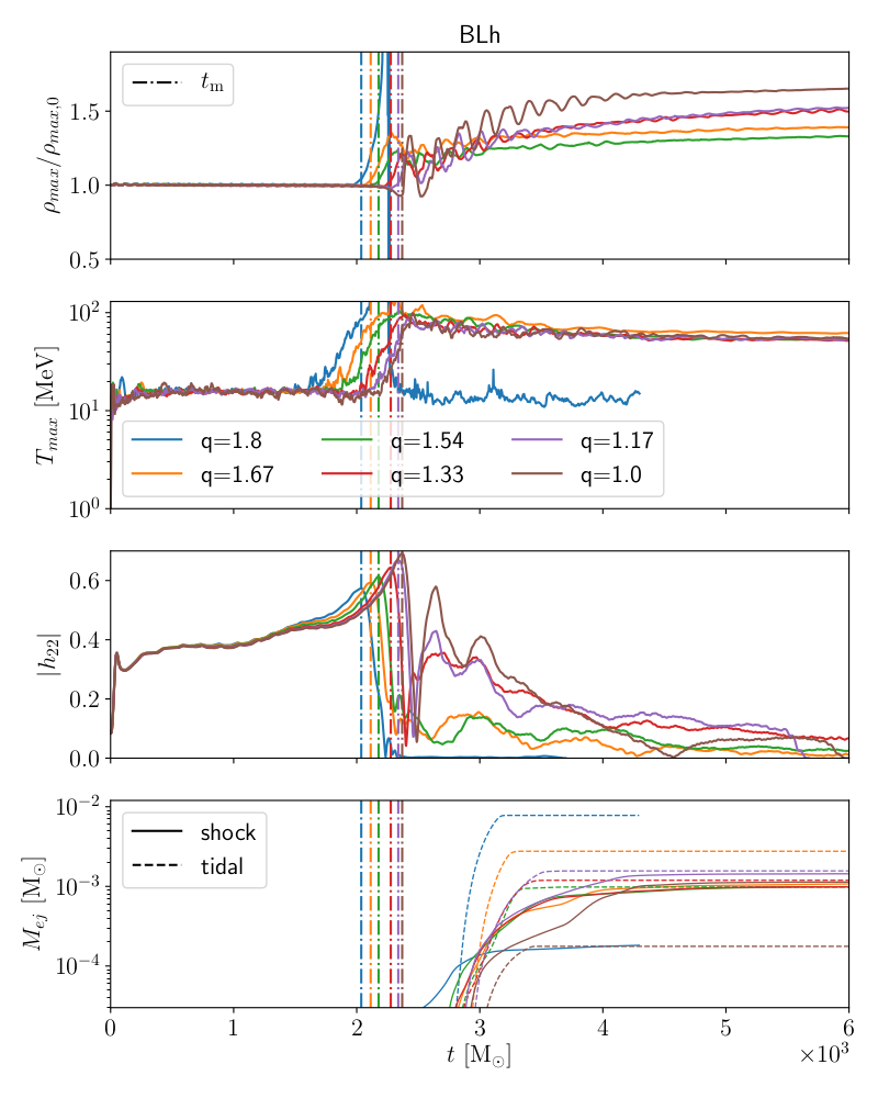
Figure 19: Main scalar quantities for several different mass ratio models with BLh. Each simulation presented here is run at grid setup LR. In the first panel we show the evolution of the maximum density ($\rho_{\text{max}}/\rho_{0}$), in the second panel the evolution of the maximum temperature ($T_{\rm max}$), in the third the gravitational wave amplitude. The last panel shows the evolution of the total mass of the dynamical ejecta: with solid and dashed lines we highlight the contribution of shock- and tidal-driven components respectively. The vertical dashed lines in all panels indicate merger time for each simulation.

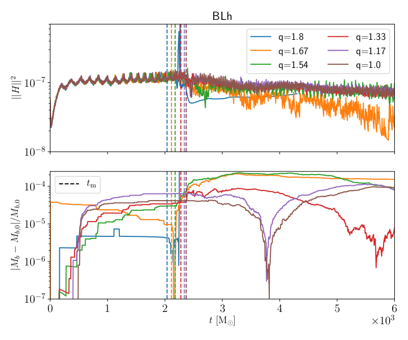
Figure 20: Simulation control quantities for several different mass ratio models with BLh. In the first panel we show the 2-norm of the Hamiltonian constrain ($||H||^{2}$), while in the second panel we show the deviation of the total baryonic mass ($M_{b}$) from the initial data value ($M_{b,0}$).

Appendix C Quasiuniversal relations of binding energy and angular momentum at merger

In this appendix, we introduce NR fit formulae for binding energy $e^{\rm mrg}_{b}$ and angular momentum $j^{\rm mrg}$ for BNS at the moment of merger. The fits are calibrated on 172 NR simulations with $q\leq 1.5$ extracted from the CoRe database Dietrich et al. (2018); Radice et al. (2018d). The fitted relations are a rational functions parametrized with $\xi$, introduced in Eq. (8),

$$F(\xi)=F_{0}\,\frac{1+n_{1}\xi+n_{2}\xi^{2}}{1+d_{1}\xi+d_{2}\xi^{2}}\,.$$ (16)

For the binding energy $e^{\rm mrg}_{b}$, the analyzed data span a range from -0.065 to -0.043, and the best-fit coefficients are $F_{0}=0.20179$, $n_{1}=-114.42$, $n_{2}=-0.39976$, $d_{1}=286.19$, $d_{2}=2.2687$ and $c=1285.2$, where $c$ is defined in Eq. (8). The calibration has $\chi^{2}=6.8\times 10^{-3}$ and the intrinsic uncertainty of the fit corresponds to ${\sim}7\%$ of the estimation, referring to the 90% credible regions. Regarding the angular momentum $j^{\rm mrg}$, the data have values between 3.3 and 3.8 and the best-fit coefficients are $F_{0}=0.028862$, $n_{1}=40.884$, $n_{2}=0.072754$, $d_{1}=0.352$, $d_{2}=0.0004703$ and $c=1325.2$. In this calibration, we obtain $\chi^{2}=1.9\times 10^{-2}$ and the fit has an uncertainty of ${\sim}3\%$ within the 90% credible region.

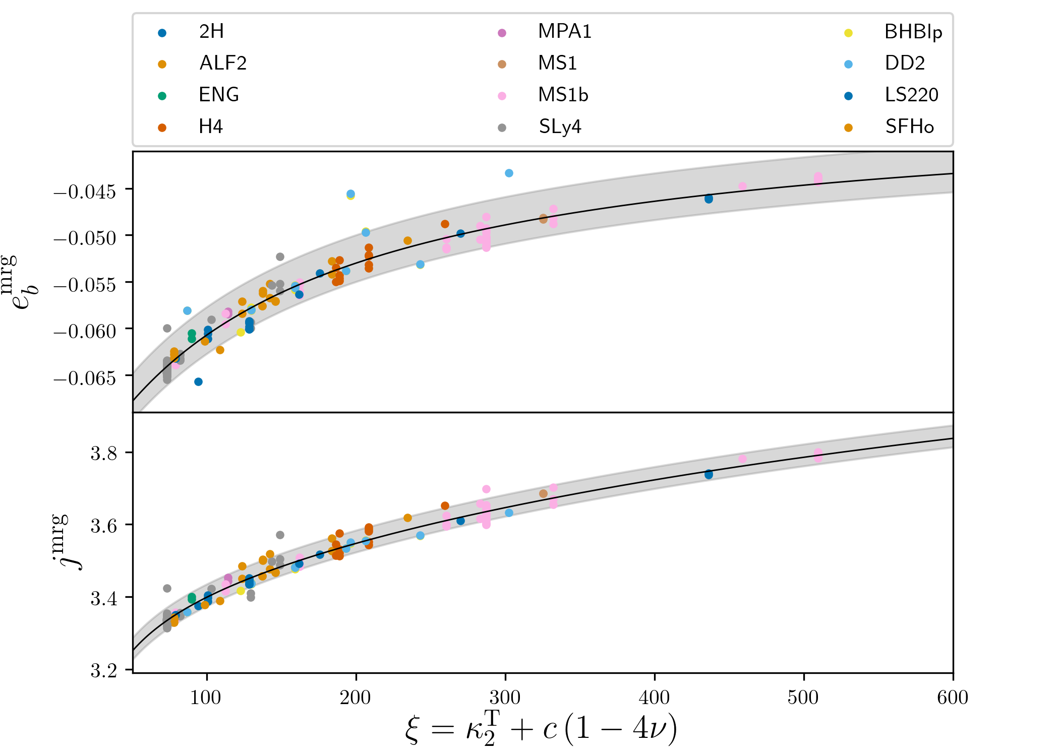
Figure 21: NR fits for binding energy $e^{\rm mrg}_{b}=E^{\rm mrg}_{b}/(\nu M)$ and angular momentum $j^{\rm mrg}=J^{\rm mrg}/(\nu M^{2})$ of a BNS at the moment of merger. The employed data are extracted from NR simulations of BNS with $q<1.5$ included in the CoRe database.

References

- Abbott et al. (2017a) Abbott B. P., et al., 2017a, Phys. Rev. Lett., 119, 161101
- Abbott et al. (2017b) Abbott B. P., et al., 2017b, Astrophys. J., 848, L12
- Abbott et al. (2018) Abbott B. P., et al., 2018, Phys. Rev. Lett., 121, 161101
- Abbott et al. (2019a) Abbott B. P., et al., 2019a, Phys. Rev., X9, 011001
- Abbott et al. (2019b) Abbott B. P., et al., 2019b, Phys. Rev., X9, 031040
- Abbott et al. (2020) Abbott B., et al., 2020, Astrophys. J. Lett., 892, L3
- Agathos et al. (2020) Agathos M., Zappa F., Bernuzzi S., Perego A., Breschi M., Radice D., 2020, Phys. Rev., D101, 044006
- Akcay et al. (2019) Akcay S., Bernuzzi S., Messina F., Nagar A., Ortiz N., Rettegno P., 2019, Phys. Rev., D99, 044051
- Ansorg et al. (2004) Ansorg M., Brügmann B., Tichy W., 2004, Phys. Rev., D70, 064011
- Antoniadis et al. (2013) Antoniadis J., Freire P. C., Wex N., Tauris T. M., Lynch R. S., et al., 2013, Science, 340, 6131
- Baiotti et al. (2009) Baiotti L., Bernuzzi S., Corvino G., De Pietri R., Nagar A., 2009, Phys. Rev., D79, 024002
- Baker et al. (2006) Baker J. G., Centrella J., Choi D.-I., Koppitz M., van Meter J., 2006, Phys. Rev. Lett., 96, 111102
- Barbieri et al. (2020) Barbieri C., Salafia O. S., Perego A., Colpi M., Ghirlanda G., 2020, Eur. Phys. J., A56, 8
- Bauswein et al. (2013a) Bauswein A., Baumgarte T., Janka H. T., 2013a, Phys.Rev.Lett., 111, 131101
- Bauswein et al. (2013b) Bauswein A., Goriely S., Janka H.-T., 2013b, Astrophys.J., 773, 78
- Berger & Colella (1989) Berger M. J., Colella P., 1989, Journal of Computational Physics, 82, 64
- Berger & Oliger (1984) Berger M. J., Oliger J., 1984, J.Comput.Phys., 53, 484
- Bernuzzi & Hilditch (2010) Bernuzzi S., Hilditch D., 2010, Phys. Rev., D81, 084003
- Bernuzzi et al. (2012) Bernuzzi S., Nagar A., Thierfelder M., Brügmann B., 2012, Phys.Rev., D86, 044030
- Bernuzzi et al. (2014) Bernuzzi S., Dietrich T., Tichy W., Brügmann B., 2014, Phys.Rev., D89, 104021
- Bernuzzi et al. (2015a) Bernuzzi S., Nagar A., Dietrich T., Damour T., 2015a, Phys.Rev.Lett., 114, 161103
- Bernuzzi et al. (2015b) Bernuzzi S., Dietrich T., Nagar A., 2015b, Phys. Rev. Lett., 115, 091101
- Bernuzzi et al. (2016) Bernuzzi S., Radice D., Ott C. D., Roberts L. F., Moesta P., Galeazzi F., 2016, Phys. Rev., D94, 024023
- Binnington & Poisson (2009) Binnington T., Poisson E., 2009, Phys. Rev., D80, 084018
- Bombaci & Logoteta (2018) Bombaci I., Logoteta D., 2018, Astron. Astrophys., 609, A128
- Bombaci et al. (1993) Bombaci I., Kuo T. T. S., Lombardo U., 1993, Phys. Lett., B311, 9
- Breschi et al. (2019) Breschi M., Bernuzzi S., Zappa F., Agathos M., Perego A., Radice D., Nagar A., 2019, Phys. Rev., D100, 104029
- Brügmann et al. (2008) Brügmann B., Gonzalez J. A., Hannam M., Husa S., Sperhake U., et al., 2008, Phys.Rev., D77, 024027
- Bulla (2019) Bulla M., 2019, Mon. Not. Roy. Astron. Soc., 489, 5037
- Campanelli et al. (2006) Campanelli M., Lousto C. O., Marronetti P., Zlochower Y., 2006, Phys. Rev. Lett., 96, 111101
- Cromartie et al. (2019) Cromartie H. T., et al., 2019, Nat. Astron., 4, 72
- Damour (1983) Damour T., 1983, in Deruelle N., Piran T., eds, Gravitational Radiation. North-Holland, Amsterdam, pp 59–144
- Damour & Nagar (2009) Damour T., Nagar A., 2009, Phys. Rev., D80, 084035
- Damour & Nagar (2010) Damour T., Nagar A., 2010, Phys. Rev., D81, 084016
- Damour et al. (2012a) Damour T., Nagar A., Pollney D., Reisswig C., 2012a, Phys.Rev.Lett., 108, 131101
- Damour et al. (2012b) Damour T., Nagar A., Villain L., 2012b, Phys.Rev., D85, 123007
- Danielewicz & Lee (2014) Danielewicz P., Lee J., 2014, Nucl. Phys., A922, 1
- De et al. (2018) De S., Finstad D., Lattimer J. M., Brown D. A., Berger E., Biwer C. M., 2018, Phys. Rev. Lett., 121, 091102
- Demorest et al. (2010) Demorest P., Pennucci T., Ransom S., Roberts M., Hessels J., 2010, Nature, 467, 1081
- Desai et al. (2019) Desai D., Metzger B. D., Foucart F., 2019, Mon. Not. Roy. Astron. Soc., 485, 4404
- Dietrich & Bernuzzi (2015) Dietrich T., Bernuzzi S., 2015, Phys.Rev., D91, 044039
- Dietrich & Brügmann (2014) Dietrich T., Brügmann B., 2014, J.Phys.Conf.Ser., 490, 012155
- Dietrich et al. (2015) Dietrich T., Moldenhauer N., Johnson-McDaniel N. K., Bernuzzi S., Markakis C. M., Brügmann B., Tichy W., 2015, Phys. Rev., D92, 124007
- Dietrich et al. (2017) Dietrich T., Ujevic M., Tichy W., Bernuzzi S., Brügmann B., 2017, Phys. Rev., D95, 024029
- Dietrich et al. (2018) Dietrich T., et al., 2018, Class. Quant. Grav., 35, 24LT01
- Dimmelmeier et al. (2006) Dimmelmeier H., Stergioulas N., Font J. A., 2006, Mon. Not. Roy. Astron. Soc., 368, 1609
- Douchin & Haensel (2001) Douchin F., Haensel P., 2001, Astron. Astrophys., 380, 151
- Eichler et al. (2015) Eichler M., et al., 2015, Astrophys. J., 808, 30
- Endrizzi et al. (2018) Endrizzi A., Logoteta D., Giacomazzo B., Bombaci I., Kastaun W., Ciolfi R., 2018, Phys. Rev., D98, 043015
- Endrizzi et al. (2020) Endrizzi A., et al., 2020, Eur.Phys.J.A, 56, 15
- Favata (2014) Favata M., 2014, Phys.Rev.Lett., 112, 101101
- Flanagan & Hinderer (2008) Flanagan E. E., Hinderer T., 2008, Phys.Rev., D77, 021502
- Foley et al. (2020) Foley R. J., Coulter D. A., Kilpatrick C. D., Piro A. L., Ramirez-Ruiz E., Schwab J., 2020, arXiv e-prints, p. arXiv:2002.00956
- Fontes et al. (2020) Fontes C., Fryer C., Hungerford A., Wollaeger R., Korobkin O., 2020, Mon. Not. Roy. Astron. Soc., 493, 4143
- Foucart et al. (2018) Foucart F., Duez M. D., Kidder L. E., Nguyen R., Pfeiffer H. P., Scheel M. A., 2018, Phys. Rev., D98, 063007
- Gaigalas et al. (2019) Gaigalas G., Kato D., Rynkun P., Radziute L., Tanaka M., 2019, Astrophys. J. Suppl., 240, 29
- Goodale et al. (2003) Goodale T., Allen G., Lanfermann G., Massó J., Radke T., Seidel E., Shalf J., 2003, in Vector and Parallel Processing – VECPAR’2002, 5th International Conference, Lecture Notes in Computer Science. Springer, Berlin
- Gottlieb & Ketcheson (2009) Gottlieb S., Ketcheson David I.and Shu C.-W., 2009, Journal of Scientific Computing, 38, 251
- Gourgoulhon et al. (2001) Gourgoulhon E., Grandclement P., Taniguchi K., Marck J.-A., Bonazzola S., 2001, Phys.Rev., D63, 064029
- Hannam et al. (2007) Hannam M., Husa S., Pollney D., Brügmann B., O’Murchadha N., 2007, Phys. Rev. Lett., 99, 241102
- Hannam et al. (2008) Hannam M., Husa S., Ohme F., Brügmann B., O’Murchadha N., 2008, Phys.Rev., D78, 064020
- Hempel & Schaffner-Bielich (2010) Hempel M., Schaffner-Bielich J., 2010, Nucl. Phys., A837, 210
- Hilditch et al. (2013) Hilditch D., Bernuzzi S., Thierfelder M., Cao Z., Tichy W., Bruegmann B., 2013, Phys. Rev., D88, 084057
- Hinderer (2008) Hinderer T., 2008, Astrophys.J., 677, 1216
- Hotokezaka et al. (2011) Hotokezaka K., Kyutoku K., Okawa H., Shibata M., Kiuchi K., 2011, Phys.Rev., D83, 124008
- Hotokezaka et al. (2013) Hotokezaka K., Kiuchi K., Kyutoku K., Okawa H., Sekiguchi Y.-i., et al., 2013, Phys.Rev., D87, 024001
- Kaplan et al. (2014) Kaplan J., Ott C., O’Connor E., Kiuchi K., Roberts L., et al., 2014, Astrophys.J., 790, 19
- Kasen et al. (2013) Kasen D., Badnell N. R., Barnes J., 2013, Astrophys. J., 774, 25
- Kastaun & Galeazzi (2015) Kastaun W., Galeazzi F., 2015, Phys.Rev., D91, 064027
- Kawaguchi et al. (2016) Kawaguchi K., Kyutoku K., Shibata M., Tanaka M., 2016, Astrophys. J., 825, 52
- Kawaguchi et al. (2020) Kawaguchi K., Shibata M., Tanaka M., 2020, ApJ, 889, 171
- Kiuchi et al. (2009) Kiuchi K., Sekiguchi Y., Shibata M., Taniguchi K., 2009, Phys. Rev., D80, 064037
- Kiuchi et al. (2010) Kiuchi K., Sekiguchi Y., Shibata M., Taniguchi K., 2010, Phys. Rev. Lett., 104, 141101
- Kiuchi et al. (2018) Kiuchi K., Kyutoku K., Sekiguchi Y., Shibata M., 2018, Phys. Rev., D97, 124039
- Kiuchi et al. (2019) Kiuchi K., Kyutoku K., Shibata M., Taniguchi K., 2019, Astrophys. J., 876, L31
- Kiziltan et al. (2013) Kiziltan B., Kottas A., De Yoreo M., Thorsett S. E., 2013, Astrophys. J., 778, 66
- Koeppel et al. (2019) Koeppel S., Bovard L., Rezzolla L., 2019, Astrophys. J., 872, L16
- Korobkin et al. (2020) Korobkin O., et al., 2020, arXiv e-prints, p. arXiv:2004.00102
- Kostadt & Liu (2000) Kostadt P., Liu M., 2000, Phys. Rev. D, 62, 023003
- Kyutoku et al. (2015) Kyutoku K., Ioka K., Okawa H., Shibata M., Taniguchi K., 2015, Phys. Rev., D92, 044028
- Kyutoku et al. (2020) Kyutoku K., Fujibayashi S., Hayashi K., Kawaguchi K., Kiuchi K., Shibata M., Tanaka M., 2020, Astrophys. J., 890, L4
- Lattimer (2012) Lattimer J. M., 2012, Ann. Rev. Nucl. Part. Sci., 62, 485
- Lattimer & Lim (2013) Lattimer J. M., Lim Y., 2013, Astrophys. J., 771, 51
- Lattimer & Swesty (1991) Lattimer J. M., Swesty F. D., 1991, Nucl. Phys., A535, 331
- Lehner et al. (2016) Lehner L., Liebling S. L., Palenzuela C., Caballero O. L., O’Connor E., Anderson M., Neilsen D., 2016, Class. Quant. Grav., 33, 184002
- Loffler et al. (2012) Loffler F., et al., 2012, Class. Quant. Grav., 29, 115001
- Logoteta et al. (2016) Logoteta D., Bombaci I., Kievsky A., 2016, Phys. Rev., C94, 064001
- Machleidt & Entem (2011) Machleidt R., Entem D. R., 2011, Phys. Rept., 503, 1
- Metzger et al. (2010) Metzger B. D., Arcones A., Quataert E., Martinez-Pinedo G., 2010, Mon. Not. Roy. Astron. Soc., 402, 2771
- Miller et al. (2019) Miller M. C., et al., 2019, Astrophys. J., 887, L24
- Nagy et al. (1994) Nagy G. B., Ortiz O. E., Reula O. A., 1994, Journal of Mathematical Physics, 35, 4334
- Nedora et al. (2019) Nedora V., Bernuzzi S., Radice D., Perego A., Endrizzi A., Ortiz N., 2019, Astrophys. J., 886, L30
- Neilsen et al. (2014) Neilsen D., Liebling S. L., Anderson M., Lehner L., O’Connor E., et al., 2014, Phys.Rev., D89, 104029
- Ozel et al. (2012) Ozel F., Psaltis D., Narayan R., Villarreal A. S., 2012, Astrophys. J., 757, 55
- Palenzuela et al. (2015) Palenzuela C., Liebling S. L., Neilsen D., Lehner L., Caballero O. L., O’Connor E., Anderson M., 2015, Phys. Rev., D92, 044045
- Passamonti et al. (2007) Passamonti A., Stergioulas N., Nagar A., 2007, Phys. Rev., D75, 084038
- Perego et al. (2017) Perego A., Radice D., Bernuzzi S., 2017, Astrophys. J., 850, L37
- Perego et al. (2019) Perego A., Bernuzzi S., Radice D., 2019, Eur. Phys. J., A55, 124
- Piarulli et al. (2016) Piarulli M., et al., 2016, Phys. Rev., C94, 054007
- Pollney et al. (2011) Pollney D., Reisswig C., Schnetter E., Dorband N., Diener P., 2011, Phys. Rev., D83, 044045
- Radice (2017) Radice D., 2017, Astrophys. J., 838, L2
- Radice (2020) Radice D., 2020, arXiv e-prints, p. arXiv:2005.09002
- Radice & Rezzolla (2012) Radice D., Rezzolla L., 2012, Astron. Astrophys., 547, A26
- Radice et al. (2014a) Radice D., Rezzolla L., Galeazzi F., 2014a, Class.Quant.Grav., 31, 075012
- Radice et al. (2014b) Radice D., Rezzolla L., Galeazzi F., 2014b, Mon.Not.Roy.Astron.Soc., 437, L46
- Radice et al. (2016) Radice D., Galeazzi F., Lippuner J., Roberts L. F., Ott C. D., Rezzolla L., 2016, Mon. Not. Roy. Astron. Soc., 460, 3255
- Radice et al. (2017) Radice D., Bernuzzi S., Del Pozzo W., Roberts L. F., Ott C. D., 2017, Astrophys. J., 842, L10
- Radice et al. (2018a) Radice D., Perego A., Bernuzzi S., Zhang B., 2018a, Mon. Not. Roy. Astron. Soc., 481, 3670
- Radice et al. (2018b) Radice D., Perego A., Zappa F., Bernuzzi S., 2018b, Astrophys. J., 852, L29
- Radice et al. (2018c) Radice D., Perego A., Hotokezaka K., Bernuzzi S., Fromm S. A., Roberts L. F., 2018c, Astrophys. J. Lett., 869, L35
- Radice et al. (2018d) Radice D., Perego A., Hotokezaka K., Fromm S. A., Bernuzzi S., Roberts L. F., 2018d, Astrophys. J., 869, 130
- Radice et al. (2020) Radice D., Bernuzzi S., Perego A., 2020, arXiv e-prints, p. arXiv:2002.03863
- Rawls et al. (2011) Rawls M. L., Orosz J. A., McClintock J. E., Torres M. A. P., Bailyn C. D., Buxton M. M., 2011, Astrophys. J., 730, 25
- Reisswig et al. (2013a) Reisswig C., Ott C., Abdikamalov E., Haas R., Mösta P., et al., 2013a, Phys.Rev.Lett., 111, 151101
- Reisswig et al. (2013b) Reisswig C., Haas R., Ott C. D., Abdikamalov E., Mösta P., Pollney D., Schnetter E., 2013b, Phys. Rev., D87, 064023
- Rezzolla et al. (2010) Rezzolla L., Baiotti L., Giacomazzo B., Link D., Font J. A., 2010, Class. Quant. Grav., 27, 114105
- Riley et al. (2019) Riley T. E., et al., 2019, Astrophys. J., 887, L21
- Rosswog (2007) Rosswog S., 2007, Mon. Not. Roy. Astron. Soc., 376, L48
- Rosswog & Liebendoerfer (2003) Rosswog S., Liebendoerfer M., 2003, Mon.Not.Roy.Astron.Soc., 342, 673
- Rosswog et al. (2017) Rosswog S., Feindt U., Korobkin O., Wu M. R., Sollerman J., Goobar A., Martinez-Pinedo G., 2017, Class. Quant. Grav., 34, 104001
- Rosswog et al. (2018) Rosswog S., Sollerman J., Feindt U., Goobar A., Korobkin O., Wollaeger R., Fremling C., Kasliwal M. M., 2018, Astron. Astrophys., 615, A132
- Ruffert et al. (1996) Ruffert M. H., Janka H. T., Schäfer G., 1996, Astron. Astrophys., 311, 532
- Schneider et al. (2017) Schneider A. S., Roberts L. F., Ott C. D., 2017, Phys. Rev., C96, 065802
- Schnetter et al. (2004) Schnetter E., Hawley S. H., Hawke I., 2004, Class.Quant.Grav., 21, 1465
- Schnetter et al. (2007) Schnetter E., Ott C. D., Allen G., Diener P., Goodale T., Radke T., Seidel E., Shalf J., 2007, arXiv e-prints, p. arXiv:0707.1607
- Sekiguchi et al. (2011a) Sekiguchi Y., Kiuchi K., Kyutoku K., Shibata M., 2011a, Phys.Rev.Lett., 107, 051102
- Sekiguchi et al. (2011b) Sekiguchi Y., Kiuchi K., Kyutoku K., Shibata M., 2011b, Phys.Rev.Lett., 107, 211101
- Sekiguchi et al. (2015) Sekiguchi Y., Kiuchi K., Kyutoku K., Shibata M., 2015, Phys.Rev., D91, 064059
- Sekiguchi et al. (2016) Sekiguchi Y., Kiuchi K., Kyutoku K., Shibata M., Taniguchi K., 2016, Phys. Rev., D93, 124046
- Shapiro (2017) Shapiro S. L., 2017, Phys. Rev., D95, 101303
- Shibata & Taniguchi (2006) Shibata M., Taniguchi K., 2006, Phys.Rev., D73, 064027
- Shibata et al. (2003) Shibata M., Taniguchi K., Uryu K., 2003, Phys. Rev., D68, 084020
- Steiner et al. (2013) Steiner A. W., Hempel M., Fischer T., 2013, Astrophys. J., 774, 17
- Stergioulas et al. (2011) Stergioulas N., Bauswein A., Zagkouris K., Janka H.-T., 2011, Mon.Not.Roy.Astron.Soc., 418, 427
- Swiggum et al. (2015) Swiggum J. K., et al., 2015, Astrophys. J., 805, 156
- Tanaka et al. (2014) Tanaka M., Hotokezaka K., Kyutoku K., Wanajo S., Kiuchi K., Sekiguchi Y., Shibata M., 2014, Astrophys. J., 780, 31
- Tanaka et al. (2019) Tanaka M., Kato D., Gaigalas G., Kawaguchi K., 2019, arXiv e-prints, p. arXiv:1906.08914
- Thierfelder et al. (2011a) Thierfelder M., Bernuzzi S., Hilditch D., Brügmann B., Rezzolla L., 2011a, Phys.Rev., D83, 064022
- Thierfelder et al. (2011b) Thierfelder M., Bernuzzi S., Brügmann B., 2011b, Phys.Rev., D84, 044012
- Thornburg (2004) Thornburg J., 2004, Class. Quant. Grav., 21, 743
- Villar et al. (2017) Villar V. A., et al., 2017, Astrophys. J., 851, L21
- Weymann (1967) Weymann H. D., 1967, American Journal of Physics, 35, 488
- Wollaeger et al. (2018) Wollaeger R. T., et al., 2018, Mon. Not. Roy. Astron. Soc., 478, 3298
- Zappa (2018) Zappa F., 2018, Master’s thesis, Parma U, Italy
- Zappa et al. (2018) Zappa F., Bernuzzi S., Radice D., Perego A., Dietrich T., 2018, Phys. Rev. Lett., 120, 111101
- van Meter et al. (2006) van Meter J. R., Baker J. G., Koppitz M., Choi D.-I., 2006, Phys. Rev., D73, 124011