Waveform systematics in the gravitational-wave inference of
tidal parameters and equation of state from binary neutron star signals

Abstract

Gravitational-wave signals from binary neutron star coalescences carry information about the star’s equation of state in their tidal signatures. A major issue in the inference of the tidal parameters (or directly of the equation of state) is the systematic error introduced by the waveform approximants. We use a bottom-up approach based on gauge-invariant phase analysis and the Fisher information matrix to investigate waveform systematics and help identifying biases in parameter estimation. A mock analysis of 15 different binaries indicates that systematics in current waveform models dominate over statistical errors at signal-to-noise ratio (SNR) ${\gtrsim}80$. This implies biases in the inference of the reduced tidal parameter that are are larger than the statistical $90\%$ credible-intervals. For example, while the neutron-star radius could be constrained at ${\sim}5\%$ level at SNR 80, systematics can be at the ${\sim}10\%$ level. We apply our approach to GW170817 (SNR ${\sim}30$) and confirm that no significant systematic effects are present. Using an optimal frequency range for the analysis, we estimate a neutron-star radius of $12.5^{+1.1}_{-1.8}\,$km. The latter is consistent with an electromagnetic-informed prior and the recent NICER measurement. Exploring SNR ${\gtrsim}100$ in view of third-generation detectors, we find that all the current waveform models lead to differences of at least 1-sigma in the inference of the reduced tidal parameter (for any value of the latter). We conclude that current waveform models, including those from numerical relativity, are insufficient to infer the equation of state in the loudest (and potentially most informative) events that will be observed by advanced and third generation detectors.

I Introduction

The detection of GW170817 Abbott et al. (2017a), the first coalescing binary neutron star (BNS) system seen by LIGO-Virgo detectors, demonstrated how gravitational waves (GWs) can be employed as a mean to investigate the properties of cold, dense matter Radice et al. (2018); Abbott et al. (2018a); Essick et al. (2020); Abbott et al. (2020a). Parameter estimation (PE) of GW data gives direct information on the masses, spins and tidal parameters of the two objects involved in the coalescence. Matched filtering analyses are performed in the Fourier domain by matching the whitened data, i.e time series sampled at a constant sampling frequency, to a large number of template waveforms within a Bayesian framework Ghosh et al. (2016). The tools employed during PE are based on Markov-chain Monte Carlo (MCMC) methods or nested sampling algorithms Veitch et al. (2015). The template waveforms are obtained relying on approximate solutions of the two body problem in general relativity (see e.g. Refs. Flanagan and Hinderer (2008); Damour and Nagar (2010, 2011); Damour et al. (2015) and references therein). Different approximations and methods give rise to different template families, which - during the process of PE - may in principle lead to different results in the recovery of the source parameters. Errors and biases completely referable to waveform modeling choices are commonly labelled as waveform systematics, and are the main topic of the present paper.

Significant waveform systematics, larger than statistical uncertainties, have yet to be observed for binary neutron star systems: looking at the results coming from the recent observations of BNS mergers, the parameters of both GW190425 Abbott et al. (2020b) and GW170817 Abbott et al. (2019a) have been demonstrated to be largely consistent between different waveform families. However, recent studies Dudi et al. (2018); Samajdar and Dietrich (2018, 2019); Messina et al. (2019); Agathos et al. (2020); Narikawa et al. (2019); Chen et al. (2020) have pointed out that the measured tidal parameters can be strongly biased depending on the employed tidal and point mass descriptions of the waveform approximant. The agreement between the different GW models employed in the PE of the observed BNS signals is then mainly due to the relatively low signal-to-noise ratio (SNR). With the increasing sensitivities of next-generation detectors Sathyaprakash et al. (2011); Aasi et al. (2015); Abbott et al. (2018b); Harry (2010); Acernese et al. (2015); Maggiore et al. (2020), waveform systematics will affect the measurements thus leading to discordant (or inconclusive) results.

In this context, the necessity of understanding the errors introduced by waveform systematics arises. In this paper, we aim at tackling the issue for SNRs relevant for advanced and 3G detectors, and provide a bottom-up approach to guide future BNS analyses. In particular, in Sec. II we summarize the current knowledge of the theoretical tools which are employed to a-priori predict the presence of waveform systematics, we expand on the argument of Ref. Messina et al. (2019) and propose a way, inspired by Cutler and Vallisneri (2007); Favata (2014), to estimate the bias that may affect tidal parameters. In Sec. III we summarize the key features of the GW models used in our analysis, and compare them by computing their gauge-invariant phasing. In Sec. IV we perform mock PE experiments (injections) with 15 binaries having signal-to-noise ratio ${\sim}80$, to study the posterior distributions of the typical parameters of interest of a BNS merger, such as tidal deformabilities, mass ratio and spins. Differently from previous studies, we focus on injections of different masses and EOS (Cf. Dudi et al. (2018); Samajdar and Dietrich (2018, 2019) where fewer binaries have been considered) and nonspinning waveforms (See Samajdar and Dietrich (2019) for spin effects.) In particular, we discuss the impact of waveform systematics on the inference of the tidal parameters and the estimation of the radii of the single NSs. In Sec V we apply the methods developed during the previous sections to GW170817. We re-analyze the event’s data and find that analyses considering up to 1kHz are free of systematics. Finally, in Sec. VI we estimate the impact of waveform systematics for BNS events detected with third generation detectors and find that statistical errors will be comparable to waveform systematics from SNRs $>200$ for $\tilde{\Lambda}\simeq 400-1000$.

Throughout the whole paper we label the two bodies as $A,B$. We denote the component masses as $m_{A},m_{B}$, the dimensionless spins of the bodies as $\chi_{A,B}$, the total mass as $M=m_{A}+m_{B}$, and define the chirp mass of the binary as $\mathcal{M}_{c}=(m_{A}m_{B})^{3/5}/(M)^{1/5}$. We define the quadrupolar tidal parameters as

$$\Lambda_{A}\equiv\frac{2}{3}\,\mathcal{C}_{A}^{-5}k^{(2)}_{A},$$ (1)

where $k_{A}^{(2)}$ is the dimensionless gravitoelectric Love number Hinderer (2008); Damour and Nagar (2009), and $\mathcal{C}_{A}\equiv Gm_{A}/(c^{2}R_{A})$ is the compactness parameter. $\Lambda_{A}$ is also denoted by $\bar{\lambda}_{2}$ Yagi (2014). The quadrupole tidal parameters enters at the leading order in the phase of the waveform through the reduced tidal parameter Flanagan and Hinderer (2008); Favata (2014)

$$\tilde{\Lambda}=\frac{16}{13}\frac{(m_{A}+12m_{B})m_{A}^{4}\Lambda_{A}}{M^{5}}+(A\leftrightarrow B)\,.$$ (2)

We often switch between mass-rescaled quantities in geometrical units $c=G=1$ and physical units. Since $GM_{\odot}\simeq 4.925490947\,\mu$s or ${\simeq}1.476625038\,$km, the dimensionless frequency $\hat{\omega}=GM\omega$ relates to the frequency in Hz by

$$f=\frac{\omega}{2\pi}\simeq 32.3125\,\hat{\omega}\,\frac{M_{\odot}}{M}\,\mbox{kHz}\,.$$ (3)

II Origin of systematics

Waveform systematics are intrinsically related to the concept of measurability of the waveform parameters. They arise when the differences due to template choice are larger than those induced by noise fluctuations in the detector and statistical uncertainties, i.e when the distributions of the estimated parameters $\bar{\bm{\theta}}$ have a width $\sigma_{\bm{\theta}}$ smaller than the differences $\Delta\bm{\theta}$ induced by waveform models. In this section we highlight, with basic analytical arguments, that the systematics on tidal parameters crucially depend on the frequency regime at which the measurement is effectively performed.

Optimal gravitational-wave data analysis of compact binaries are based on matched-filtering techniques in which the data are “best matched” to waveform templates Owen and Sathyaprakash (1999). The accuracy requirements on the waveforms used in the matched filtering depend on whether waveform models are employed for detection or parameter estimation. In the former case, waveforms are required to be only effectual while in the latter they are required to be faithful Damour et al. (1998). To quantify these concepts, it is necessary to introduce a metric in the waveform space in order to measure how close two waveforms are. The basic quantity used in in GW analysis theory is the Wiener inner product between two waveforms $h(t)$ and $k(t)$, defined by

$$(h|k)=4\Re\int\frac{\tilde{h}(f)\,\tilde{k}^{*}(f)}{S_{n}(f)}\,{\rm d}f\,,$$ (4)

where $\tilde{h}(f)$ is the Fourier transform of $h(t)$ and $S_{n}(f)$ is the power spectral density (PSD) of the detector. The faithfulness (or match) is the normalized and noise-weighted inner product

$$\mathcal{F}=\max_{t_{c},\phi_{c}}\frac{(h|k)}{\sqrt{(h|h)(k|k)}}\,,$$ (5)

where $t_{c},\phi_{c}$ are respectively the time and phase of the waveform at a reference time. The match $\mathcal{F}$ defines an “angle” in the waveform space; $\mathcal{F}=1$ indicates perfect overlap between $h$ and $k$. The mismatch $\bar{\mathcal{F}}=1-\mathcal{F}$ gives the loss in signal-to-noise ratio (squared) when the waveforms are aligned in time and phase. Accuracy requirements for both detection and PE can be expressed in terms of $\mathcal{F}$ . A mismatch of $\bar{\mathcal{F}}=0.03$ corresponds to ${\sim}10$% of detection losses Lindblom et al. (2008), which is assumed as the effectualness condition for a template bank. Necessary conditions for faithful waveform models can be expressed in terms of $\mathcal{F}$ Lindblom et al. (2008); Damour et al. (2011) (see below).

Generally, the parameters of a GW signal are measured using matched-filtering techniques within a Bayesian framework Veitch et al. (2015). Defining $\tilde{d}(f)=\tilde{A}_{d}(f)e^{i\Psi_{d}(f)}$ as the target (injected or measured) strain of data, $\tilde{h}(f,\bm{\theta})=\tilde{A}_{h}(f,\bm{\theta})e^{i\Psi_{h}(f,\bm{\theta})}$ as the template waveform and $\bm{\theta}$ as the set of parameters on which $h$ depends, the likelihood function is

$$p(d|\bm{\theta})\propto e^{-\frac{1}{2}(d-h|d-h)}\,.$$ (6)

Writing $(d-h|d-h)=(d|d)+(h|h)-2(d|h)$, the maximization of the likelihood can be interpreted as the maximization of the matched-filtered SNR,

$$\rho=\frac{(d|h)}{\sqrt{(h|h)}}\propto\Re\int\frac{\tilde{A}_{d}\tilde{A}_{h}e^{i\Delta\Psi}}{S_{n}}{\rm d}f\,,$$ (7)

where $\Delta\Psi=\Psi_{h}-\Psi_{d}$. The SNR $\rho$ quantifies the amount of signal deposited in the recorded data $d$ that is matching a given template $h$. The optimal SNR, instead, is defined as the matched-filtered SNR computed within the assumption $d\approx h$,

$$\rho_{\rm opt}=\sqrt{(h|h)}\,.$$ (8)

This value identifies the SNR we would get if the signal were coincident with the template and the noise realization were identically zero, which is a first order approximation of the actual matched-filtered value. Indeed, assuming $d=h+n$ and expanding around small values of $n$, we get $\rho=\rho_{\rm opt}+O(n)$. GW data analysis delivers probability distributions of the sampled parameters (posteriors), which can be characterized by their maximum probability (peak) values and credible intervals. The measurements thus obtained can be affected by statistical uncertainties due to fluctuations of the detector noise, which impact the posteriors by widening the credible intervals, and systematic effects due to the waveform models employed, which can can influence PE by shifting the posterior distributions with respect to the true values.

II.1 Statistical Errors

Under the assumption of Gaussian noise, the variance $\sigma^{2}_{\theta_{i}}$ on the measurement of a generic parameter $\theta_{i}$ due to statistical errors can be computed through the Fisher information matrix $F_{ij}$ (see e.g. Cutler and Flanagan (1994); Lindblom et al. (2008); Damour et al. (2011)). Given a waveform model $\tilde{h}(f,\theta)=\tilde{A}_{h}(f)e^{i\Psi_{h}(f)}$, the element $(i,j)$ of $F$ is defined as

$$F_{ij}=(\partial_{i}h|\partial_{j}h)\simeq 4\int\frac{\tilde{A}_{h}^{2}}{S_{n}}\left(\partial_{i}\Psi_{h}\partial_{j}\Psi_{h}\right){\rm d}f,$$ (9)

where $\partial_{i}=\frac{\partial}{\partial\theta_{i}}$ and in the last equation we assume that the amplitude $\tilde{A}$ is not correlated to other parameters Cutler and Flanagan (1994); Poisson and Will (1995). The variance of the distribution of $\theta_{i}$ can then be estimated from Eq. (9) as

$$\sigma^{2}_{\theta_{i}}=(F^{-1})_{ii}\,.$$ (10)

The Fisher Matrix formalism further allows one to identify the relevant frequency ranges at which different parameters are measured. Focusing on Eq. (9), it is clear that the frequency ranges that contribute to the computation of $\sigma_{\theta_{i}}$ are those where the integrand

$$I_{ii}(f)=4\frac{\tilde{A}_{h}^{2}(f)}{S_{n}(f)}\,\Big{[}\partial_{i}\Psi_{h}(f)\,\partial_{i}\Psi_{h}(f)\Big{]}$$ (11)

is largest and different from zero. Using post-Newtonian (PN) waveforms, whose amplitude $\tilde{A}$ behaves as ${\sim}f^{-7/6}$, it is immediate to show that on a logarithmic frequency axis these integrands are of type $I_{ii}\sim f^{-4/3}S_{n}^{-1}(f)f^{p_{i}/3}$ where the exponent $p_{i}$ depends on the particular parameter considered Damour et al. (2012). For example, the chirp mass has $p_{\mathcal{M}}=-10$ and, for a fiducial equal-mass $1.4+1.4{\rm M_{\odot}}$ BNS, is entirely determined by the signal at low-frequencies ${\lesssim}30$ Hz. The symmetric mass ratio integrand has $p_{\nu}=-6$ and the SNR integrand has $p_{\rm SNR}=0$, which implies that they are given by the useful GW cycles below 50 and 100 Hz respectively for the fiducial BNS (see e.g. Fig. (3) of Damour et al. (2012) and Fig. (2) of Harry and Hinderer (2018)). By contrast, the reduced tidal parameters has $p_{\tilde{\Lambda}}=+10$, i.e. $I_{\tilde{\Lambda}\tilde{\Lambda}}\sim f^{2}/S_{n}(f)$, that indicates that the information on tides increases as ${\sim}f^{2}$ between 50 Hz and 800 Hz to then reach a finite limit at higher frequencies and decay after merger. This marked difference in the frequency support of $I_{\tilde{\Lambda}\tilde{\Lambda}}$ indicates that the measurement of $\tilde{\Lambda}$ is not strongly correlated to that of the chirp mass and mass ratio Damour et al. (2012), and that the magnitude of such a correlation decreases as signals become stronger, because the tidal contribution becomes easier to distinguish from the rest of the signal Damour et al. (2012). Nonetheless, nontidal parameters can still impact the determination of $\tilde{\Lambda}$ (see App. A): the maximum likelihood values of $\tilde{\Lambda}$ minimize the overall high-frequency phase differences $\Delta\Psi$, which can receive a non-negligible contribution from the point mass sectors of the approximants.

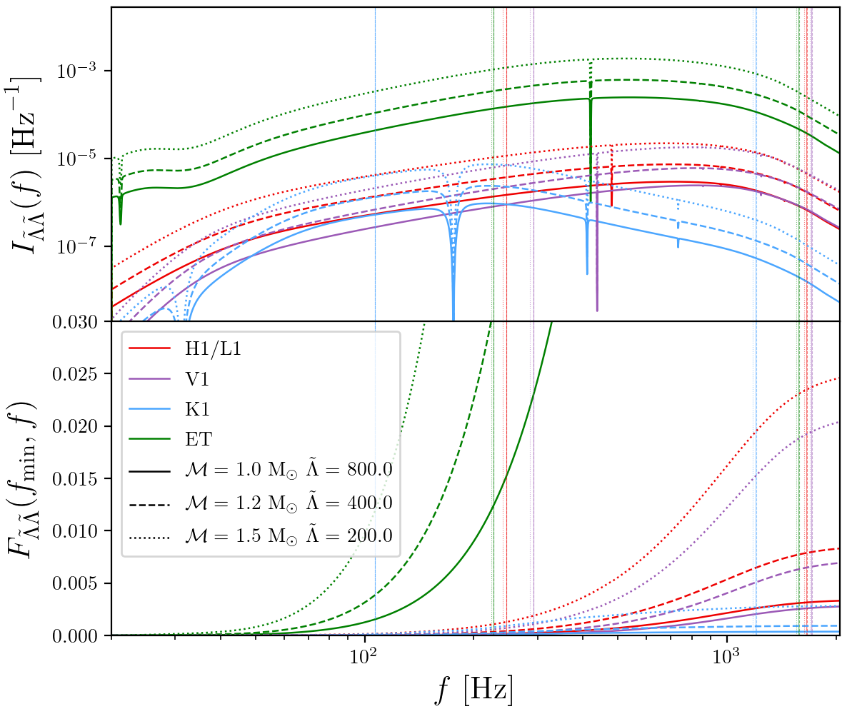
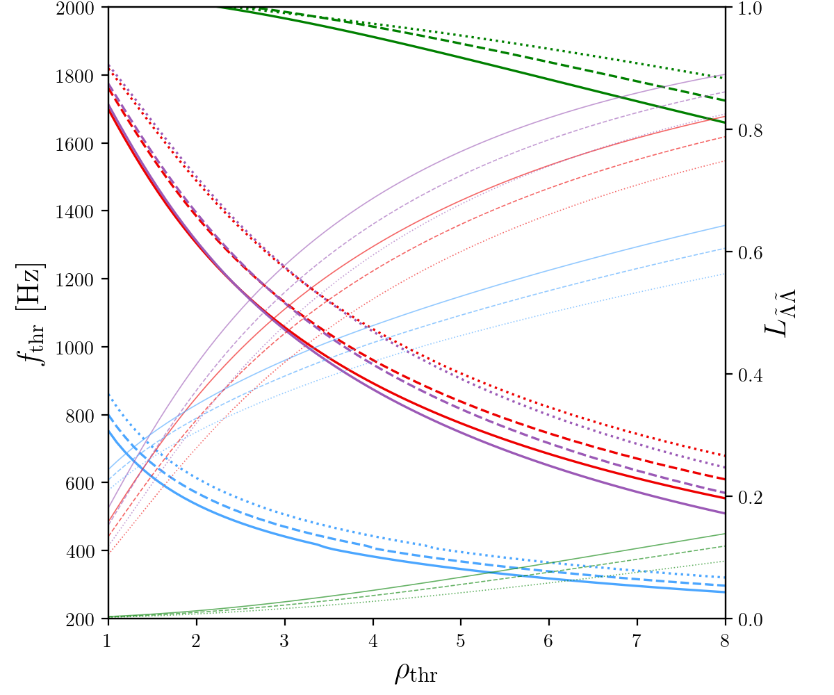
Figure 1: (Left panel) The figure shows $I_{\tilde{\Lambda}\tilde{\Lambda}}$ (top) and $F_{\tilde{\Lambda}\tilde{\Lambda}}(f_{\rm min}{=}\,20~{}{\rm Hz},f)$ (bottom) computed for different combination of $(\mathcal{M},\tilde{\Lambda})$ fixing $|s_{1}|=|s_{2}|=0$, $q=1$, $D_{L}=40~{}{\rm Mpc}$, $\iota=0$ and locating the source in the optimal sky location for the involved detector at the GPS time of GW170817 (1187008882.4). We employ ${\tt TaylorF2}$ to compute the derivatives of the phase with respect to $\tilde{\Lambda}$ and TEOBResumS to account for corrections in the waveform amplitude. The curves are estimated using design PSD expected for next-generation detectors: red lines refer to LIGO design sensitivity Aasi et al. (2015), purple lines refer to Virgo design sensitivity Acernese et al. (2015), blue lines refer to KAGRA design sensitivity Aso et al. (2013); Akutsu et al. (2019), and green lines refer to Einsten Telescope (configuration D) sensitivity Punturo et al. (2010); Hild et al. (2011). The vertical lines represent the frequencies $f_{5\%}^{\tilde{\Lambda}}$, $f_{95\%}^{\tilde{\Lambda}}$, defined in Eq. (14). (Right panel) Estimations of $f_{\rm thr}$ (thick lines) and $L_{\tilde{\Lambda}\tilde{\Lambda}}$ (thin lines) as functions of $\rho_{\rm thr}\in[1,8]$ for the cases discussed in the left panel.

The integrands $I_{ii}(f)$ can be employed to quantify the amount of information gathered on the parameter $\theta_{i}$ per frequency bin. We define the cumulative information gathered in an interval $[f_{a},f_{b}]$ of the frequency domain as

$$F_{ii}(f_{a},f_{b})=\int_{f_{a}}^{f_{b}}I_{ii}(f)\,{\rm d}f\,.$$ (12)

Values of $F_{ii}(f_{a},f_{b})$ close to zero indicate that the range $[f_{a},f_{b}]$ does not include relevant information on $\theta_{i}$. From Eq. (10) we obtain

$$\sigma_{\theta_{i}}^{2}\geq\frac{1}{F_{ii}(f_{\rm min},f_{\rm max})}\,,$$ (13)

where $f_{\rm max}$ and $f_{\rm min}$ denote the upper and lower bounds of the frequency interval chosen for the analysis.

Through the information distribution $I_{ii}(f)$ and its integral $F_{ii}(f_{\rm min},f)$ it is possible to find an optimal frequency range

where most of the information on $\theta_{i}$ is contained. We define the upper frequency $f^{i}_{X\%}$ that encloses the $X\%$ of information on the $i$-th parameter from

$$F_{ii}(f_{\rm min},f^{i}_{X\%})=\frac{X}{100}\cdot F_{ii}(f_{\rm min},f_{\rm max})\,.$$ (14)

This definition corresponds to the frequency of the $X^{\rm th}$ percentile of the information distribution $I_{ii}(f)$. It is then possible to estimate the optimal frequency range for the measurement of the $i$-th parameter as the interval that encloses the 90% of the total information, identified by the 5% and the 95% percentiles $[f_{5\%}^{i},f_{95\%}^{i}]$. Focusing on the tidal parameter $\tilde{\Lambda}$, Fig. 1 (left panel) shows the information distribution $I_{\tilde{\Lambda}\tilde{\Lambda}}(f)$ and the cumulative information $F_{\tilde{\Lambda}\tilde{\Lambda}}(f_{\rm min},f)$ computed for some exemplary binary configurations using the expected design sensitivity curves for current ground-based detectors and $f_{\rm min}=20\,$Hz. For fiducial BNS mergers with LIGO-Virgo design sensitivities, the optimal interval $[f_{5\%}^{\tilde{\Lambda}},f_{95\%}^{\tilde{\Lambda}}]$ spans a relatively high frequency range: $f_{5\%}^{\tilde{\Lambda}}\approx 300~{}{\rm Hz}$ and $f_{95\%}^{\tilde{\Lambda}}>1~{}{\rm kHz}$. Note that the above intervals are independent of the distance of the source from the detectors, i.e the same optimal frequency interval pertains to a family of signals with varying strengths and SNRs.

The key role played by distance and SNR does not lie in the determination of the optimal interval, but rather in governing the extent to which the signal can be measured and the parameters extracted. Indeed, the accuracy on the $\tilde{\Lambda}$ estimation depends crucially on the maximum frequency at which we are able to discriminate the signal from noise fluctuations. Within the assumption of $d\approx h$, it is possible to estimate the high-frequency threshold $f_{\rm thr}$ at which the signal power exceeds the noise contributions as

$$4\int_{f_{\rm thr}}^{f_{\rm max}}\frac{|\tilde{h}(f)|^{2}}{S_{n}(f)}{\rm d}f=\rho^{2}_{\rm thr}\,,$$ (15)

where $\rho_{\rm thr}$ is an arbitrary threshold value for the SNR. In the case of multiple detectors, the integral in the left-hand side of Eq. (15) has to be replaced with the summation of the integrals evaluated on the different detectors, as it is for an usual summation of SNRs. With this definition, we guarantee that the power enclosed in the frequency range $[f_{\rm thr},f_{\rm max}]$ does not exceed the threshold $\rho_{\rm thr}$. The choice of $\rho_{\rm thr}$ is a subtle issue, since this value has to quantify the amount of power due to high-frequency noise and statistical fluctuations: an overestimate will lead to the inclusion of portion of the signal as the noise contribution, while, underestimating the threshold, one may be led to believe that the signal is more informative than it really is.

In principle, $\rho_{\rm thr}$ should be a negligible value compared to the total SNR and no signal should be gathered the range $[f_{\rm thr},f_{\rm max}]$. A conservative choice is $\rho_{\rm thr}=1$, since it defines the range in which signal and noise contributions are comparable and it ensures that we are not discarding a considerable amount of signal. The choice of $\rho_{\rm thr}$ can be relaxed using the standard deviation estimated from the posterior distribution of the SNR coming from a PE analysis, since it quantifies the uncertainty on the signal power. Eq. (15) is computed using the approximation of optimal SNR, then the definition of $f_{\rm thr}$ is exact in the limit $d\to h$. In a realistic scenario, the noise contamination is non negligible, and consequently $f_{\rm thr}$ can be interpreted as an upper frequency-bound beyond which the signal power cannot exceed $\rho_{\rm thr}$; this means that, even in the best case scenario $d\approx h$, the power enclosed in the frequency range $[f_{\rm thr},f_{\rm max}]$ will always be lower (or equal, for $d=h$) than the threshold power defined by $\rho_{\rm thr}$. Once $f_{\rm thr}$ is known, it is possible to evaluate the ratio

$$L_{ii}(f_{\rm thr})=\frac{F_{ii}(f_{\rm thr},f_{\rm max})}{F_{ii}(f_{\rm min},f_{\rm max})}\,.$$ (16)

that quantifies the fractional information loss on the $i$-th parameter, since $f_{\rm thr}$ represents, by construction, the maximum frequency at which the signal is relevant. Fig. 1 (right panel) shows the estimation of $f_{\rm thr}$ and $L_{\tilde{\Lambda}\tilde{\Lambda}}$ as functions of $\rho_{\rm thr}$. As $\rho_{\rm thr}$ grows, $f_{\rm thr}(\rho_{\rm thr})$ decreases because a larger power is required to reach the increasing threshold. Conversely, $L_{\tilde{\Lambda}\tilde{\Lambda}}$ increases since, increasing $\rho_{\rm thr}$, we are considering lower values of $f_{\rm thr}$ and the support $[f_{\rm thr},f_{\rm max}]$ increases. From the arguments above it follows that if $f_{\rm thr}\ll f_{5\%}^{\tilde{\Lambda}}$, then $L_{\tilde{\Lambda}\tilde{\Lambda}}\approx 1$ and the measurement of the tidal parameter will be strongly affected by noise fluctuation and by sensitivity limits, with the possibility of an uninformative inference.

In App. B, we apply the method discussed above to the injections studied in Sec. IV, in order to prove that the injection studies are performed in an informative framework for the tidal parameter $\tilde{\Lambda}$.

Using a GW170817-like template, i.e a waveform whose intrinsic and extrinsic parameters are fixed to the maximum posterior probability of GW170817, and setting $\rho_{\rm thr}=1$, we find $f_{\rm thr}\approx 800$ Hz for LIGO design sensitivity and $f_{\rm thr}\approx 600$ Hz for Virgo design sensitivity, while for a network of three detectors $f_{\rm thr}\approx 1$ kHz and $L_{\tilde{\Lambda}\tilde{\Lambda}}\approx 20\%$ .

II.2 Systematic Errors

The probability distribution of the data $d=h+n$ containing a signal $h$ and noise is $\propto e^{-1/2(d-h|d-h)}$. Thus, the knowledge of $h$ at 1-$\sigma$ level is limited to a unit ball in Wiener space,

$$(d-h|d-h)<1\,.$$ (17)

Systematic effects due to waveform modeling have been studied in connection to Eq. (17), e.g. Lindblom et al. (2008); Damour et al. (2011). Given a waveform model $h$ to approximate the true signal $s$ recorded in the data $d=s+n$ (where $n$ denotes the noise contribution), and using the inequality $|h-d|\leq|h-s|+|s-d|=|\delta h|+|n|$ with $\delta h=s-h$, Eq. (17) (or the condition $\sigma^{2}>1$) translates into the criterion

$$(\delta h|\delta h)<\epsilon^{2}\,,$$ (18)

with $\epsilon^{2}=1$ (or smaller, for a more strict requirement). This equation corresponds to demanding that the systematics biases become of the same order as the statistical ones when the noise level is doubled Damour et al. (2011). It can be written in terms of the faithfulness as [e.g. Eq. (31) of Damour et al. (2011)]

$$\mathcal{F}>1-\frac{\epsilon^{2}}{2\,\rho^{2}}\,,$$ (19)

with $\epsilon^{2}\leq 1$. Note that sometimes it is suggested to relax this criterion by taking $\epsilon^{2}=N$, the number of intrinsic parameters of the system Chatziioannou et al. (2017). The above criteria are necessary conditions that have to be satisfied by faithful waveform models. Their violation does not guarantee the presence of biases. Indeed in Sec. IV.4 we show that all of our simulated signals lie well below the faithfulness tresholds identified by Eq. (19), though not all of them present obvious biases on $\tilde{\Lambda}$. Conversely, if a bias is present, they do not quantify how large the uncertainty on the parameters is.

The biases $\Delta\bm{\theta}=\bar{\bm{\theta}}-\bm{\theta}_{\rm true}$ between the maximum likelihood (best fit) and the true parameters due to use of a waveform model $h$ instead of the exact waveform can be estimated following Cutler and Vallisneri (2007); Favata (2014). The best fit (possibly biased) values $\bar{\bm{\theta}}$ minimize the function $g(\bm{\theta})=(d-h(\bm{\theta})|d-h(\bm{\theta}))$. Therefore, they have to be critical points of $g$, thus leading to the condition

$$(\partial_{j}h(\bar{\bm{\theta}})|d-h(\bar{\bm{\theta}}))=0\,.$$ (20)

Linearly expanding $h(\bar{\bm{\theta}})\approx h(\bm{\theta}_{\rm true})+\Delta\bm{\theta}^{j}\partial_{j}h(\bm{\theta}_{\rm true})$ and inserting it in (20) one finds that

$$\Delta\bm{\theta}^{i}=(F^{-1}(\bm{\theta}_{\rm true}))^{ij}(\partial_{j}h(\bm{\theta}_{\rm true})|d-h(\bm{\theta}_{\rm true}))$$ (21)

This equation can be reconducted to the accuracy criterion of Eq. (18). Indeed, recalling that $\sigma^{2}_{ij}=(F^{-1})_{ij}$, we can write

$$(\sigma^{2}_{ij}(\bm{\theta}_{\rm true}))^{-1}\Delta\bm{\theta}^{i}=(\partial_{j}h(\bm{\theta}_{\rm true})|d-h(\bm{\theta}_{\rm true}))$$ (22)

multiplying both sides by $\Delta\bm{\theta}^{j}$, recalling that $h(\bar{\bm{\theta}})\approx h(\bm{\theta}_{\rm true})+\Delta\bm{\theta}^{j}\partial_{j}h(\bm{\theta}_{\rm true})$ and approximating $d\approx h(\bar{\bm{\theta}})$ immediately gives

$$(\sigma^{2}_{ij}(\bm{\theta}_{\rm true}))^{-1}\Delta\bm{\theta}^{i}\Delta\bm{\theta}^{j}\approx(d-h(\bm{\theta}_{\rm true})|d-h(\bm{\theta}_{\rm true}))$$ (23)

Comparing Eq. (18) to Eq. (23) we note that indeed the validity of the former implies that the systematic biases $\Delta\bm{\theta}^{i}$ are smaller than uncertainties due to statistical fluctuations, as expected.

Estimates of the parameters bias using Eq. (21) require knowledge of the derivatives of the waveform model with respect to the parameters. These quantities, however, are nontrivial to evaluate for more sophisticated semi-analytical approximants. One might then try to directly minimize the function $g(\bm{\theta})$. This in turn requires the minimization of an integral in the multi-dimensional space of the binary parameters, which can be computationally very expensive. However, we are interested in the bias in the reduced tidal parameter and thus assume that (i) the correlation with the other parameters can be neglected; (ii) the largest biased parameter is $\tilde{\Lambda}$. The former assumption roughly holds if the SNR is sufficiently high (see above); the latter if the point-mass waveforms are sufficiently accurate at low frequencies. In these conditions, minimizing the likelihood over the whole parameter space simply reduces to computing

$$\min_{\tilde{\Lambda}}(d-h({\tilde{\Lambda}})|d-h(\tilde{\Lambda}))$$ (24)

over a one-dimensional interval of $\tilde{\Lambda}$ values, assuming that all other intrinsic parameters are correclty estimated. While such a minimization has little practical use for GW PE, as the true parameters $\bm{\theta}_{\rm true}$ are unknown, it can nonetheless be used to estimate - known the parameters associated to one particular model - the resulting value of $\tilde{\Lambda}$ that one would get by repeating PE with a different waveform model. Note the new model can disagree with the previous one also in the point-mass and spin sector as assumption (ii) only requires the two models to agree in the low-frequency limit. In Sec. IV.4 we apply this estimate to injection experiments. We find that it is able to correctly capture the behavior of the different approximants studied, and that the estimated values of $\tilde{\Lambda}$ (henceforth denoted as $\tilde{\Lambda}_{E}$) always fall within the $90\%$ credible intervals of the recovered posterior distributions, with the exception of few borderline cases where $\tilde{\Lambda}_{E}$ is nonetheless extremely close to the upper $95^{\rm th}$ percentile. In Sec. VI, instead, we apply Eq. (23) to two state-of-the-art approximants to estimate the importance of waveform systematics on PE with third generation detectors.

Note that the arguments presented in this section do not address the impact of prior assumptions in GW PE, but rather focus on the maximum-likelihood estimates, which exactly coincide with the maximum (posterior) probability values only when considering uniform prior distributions. As a general rule of thumb, as long as prior assumptions are more constraining on the source parameters than the actual observational information carried by the waveform, one should expect a-priori hypotheses to play an important role in PE Favata (2014). Extreme care is then required when dealing with lower SNR signals. For example, as discussed in Kastaun and Ohme (2019), when sampling directly in the component tidal parameters $\Lambda_{A},\Lambda_{B}$ the prior on $\tilde{\Lambda}$ is not independent of the mass ratio of the binary. This, in turn, impacts the computation of credible bounds – and especially of lower bounds, which are used to claim the measurement of tides. In the limit of high SNR, instead, the mean of the posterior distribution can be shown to coincide with the maximum likelihood estimators Vallisneri (2008). Therefore, it is in this regime that the discussion presented above has to be interpreted.

III Waveform models

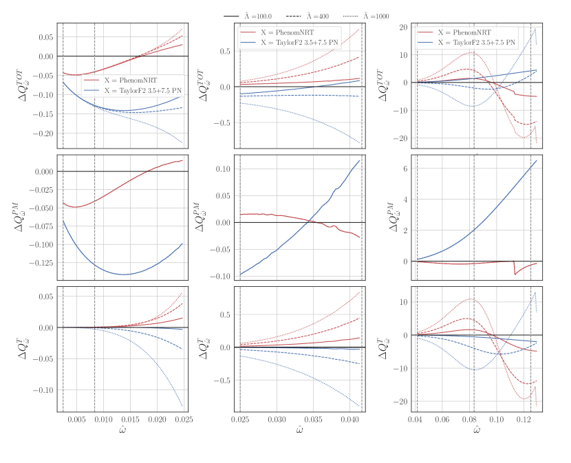
Figure 2: The $\Delta Q_{\omega}=Q_{\omega}^{TEOB}-Q_{\omega}^{X}$ function computed for three waveforms with fixed spins $\chi_{1}=\chi_{2}=0$ and varying $\tilde{\Lambda}=\{100,400,1000\}$, represented by continuous, dashed and dotted lines, respectively. $\Delta Q_{\hat{\omega}}$ is then further decomposed into its point mass $\Delta Q_{\hat{\omega}}^{\rm PM}$ (second row) and tidal $\Delta Q_{\hat{\omega}}^{\rm T}$ (third row) contributions, so that $\Delta Q_{\hat{\omega}}^{\rm TOT}=\Delta Q_{\hat{\omega}}^{\rm PM}+\Delta Q_{\hat{\omega}}^{\rm T}$, and is displayed over three different frequency ranges, roughly corresponding to the regimes in which point mass effects are dominant, comparable or negligible with respect to tidal effects. We observe that $\Delta Q_{\hat{\omega}}^{T}$ for ${\tt TaylorF2}$ and ${\tt IMRPhenomPv2NRTidal}$ have opposite behaviours, with ${\tt TaylorF2}$ being more repulsive and ${\tt IMRPhenomPv2NRTidal}$ more attractive than ${\tt TEOBResumS}$.

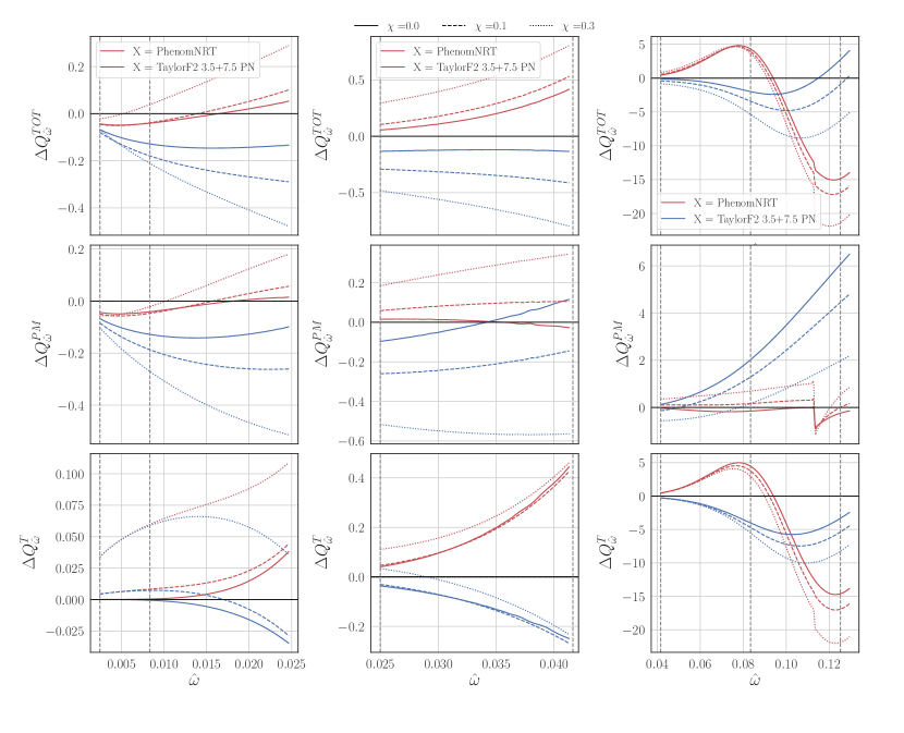
Figure 3: The $\Delta Q_{\hat{\omega}}^{\rm TOT}=Q_{\hat{\omega}}^{TEOB}-Q_{\hat{\omega}}^{X}$ function computed for three waveforms with fixed $\tilde{\Lambda}=400$ and varying spins $\chi_{1}=\chi_{2}=\{0,0.1,0.3\}$, represented by continuous, dashed and dotted lines, respectively. $\Delta Q_{\hat{\omega}}$ is then further decomposed into its point mass $\Delta Q_{\hat{\omega}}^{\rm PM}$ (second row) and tidal $\Delta Q_{\hat{\omega}}^{\rm T}$ (third row) contributions, so that $\Delta Q_{\hat{\omega}}^{\rm TOT}=\Delta Q_{\hat{\omega}}^{\rm PM}+\Delta Q_{\hat{\omega}}^{\rm T}$. Note that $\Delta Q_{\hat{\omega}}^{T}$ is comparable to $\Delta Q_{\hat{\Omega}}^{\rm PM}$ at $\hat{\omega}<0.02$. This effect can be attributed to the spin-spin interactions.

Gravitational waveform models for coalescing compact binaries aim at providing approximate solutions to the GR two-body problem. They map a set of intrinsic parameters $\bm{\theta}$, for example the mass ratio $q$, the chirp mass $\mathcal{M}_{c}$, the component dimensionless spins $(\chi_{A},\chi_{B})$ and the dimensionless tidal deformabilities $(\Lambda_{A},\Lambda_{B})$, into a time or frequency series $h(t;\bm{\theta})$ or $\tilde{h}(f;\bm{\theta})$. Post newtonian (PN) approximants Blanchet (2014); Buonanno et al. (2009) construct this mapping by analytically computing the evolution of the orbital phase $\phi(t)$ of a binary system as a perturbative expansion in a small parameter $v/c$ or $x=(v/c)^{2}$, in which $v$ is the characteristic velocity of the binary. Such models, while cheap from a computational standpoint, are typically unable to reliably describe the waveform at high frequencies Damour et al. (1998), i.e during the later phases of the evolution of the binary when $v$ becomes a comparable fraction of $c$. The effective-one-body (EOB) approach Buonanno and Damour (1999, 2000); Damour et al. (2000); Damour (2001); Damour et al. (2008, 2015); Bini et al. (2019, 2020a, 2020b) resums the PN information (both in the conservative and nonconservative part of the dynamics) so to make it reliable and predictive also in the strong-field, fast velocity regime. Once improved by NR data, this method allows one to compute the complete waveform from the early, quasi-adiabatic, inspiral up to merger and – when dealing with binary balck holes – ringdown. Finally, phenomenological models Santamaria et al. (2010); Hannam et al. (2014); Khan et al. (2016); Husa et al. (2016); London et al. (2018); García-Quirós et al. (2020); Pratten et al. (2020a, b) are constructed by first stitching together EOB-based inspirals with numerical relativity simulations, when available, and then devising an accurate, effective, interpolating representation all over the parameter space devised to be computationally efficient.

For our purposes, we choose one representative approximant from each of the three families above. In particular, our analysis will employ the PN TaylorF2 model, the EOB TEOBResumS model, and the Phenomenological IMRPhenomPv2NRTidal model. In sections VI and Appendix E we will then consider two further approximants: IMRPhenomPv2NRTidalv2 and SEOBNRv4Tsurrogate.

TaylorF2 is a frequency domain PN waveform model. The phase of the GW, obtained through a stationary phase approximation, contains point-mass effects which are fully known up to relative 3.5 PN order Buonanno et al. (2009), and include spin-spin and spin-orbit interactions Arun et al. (2009); Mikoczi et al. (2005). A higher order, parameterized, quasi–5.5PN description of nonspinning point mass effects has also been derived in Messina et al. (2019). Tidal effects can be included up to relative 7.5PN order Vines et al. (2011); Damour et al. (2012); Henry et al. (2020), while quadratic-in-spin effects were included up to 3.5PN Nagar et al. (2018). Throughout the main body of this work we will employ a 3.5PN-accurate point mass baseline, a 7.5PN description of the tidal phasing, and a 3PN description of spin-square effects.

TEOBResumS is a state-of-the-art EOB waveform model for spin-aligned coalescing compact binaries (either neutron stars or black holes) Damour and Nagar (2014); Nagar et al. (2017, 2018, 2019a, 2019b, 2020). In this paper, we focus on the tidal sector of TEOBResumS, in the form described in Nagar et al. (2018); Akcay et al. (2019); Nagar et al. (2019a). In particular, this configuration coincides with the one implemented within LALInference. The tidal sector of TEOBResumS contains contributions from the multipolar $\ell=2,3,4$ gravitoelectric and $\ell=2$ gravitomagnetic interations; the former are included in resummed form stemming from PN and gravitational-self force results Bernuzzi et al. (2015a); Akcay et al. (2019) (see also Refs. Bini et al. (2012); Bini and Damour (2014)). Equation of state-dependent self-spin effects (also known as quadrupole-monopole terms) are included at next-to-next-to-leading-order Nagar et al. (2019a) thanks to a suitable modification of the centrifugal radius introduced in Ref. Damour and Nagar (2014), so to incorporate even-in-spin effects in a way that closely mimics the structure of the Hamiltonian of a point-particle on a Kerr black hole. In addition, the models relies on the (iterated) post-adiabatic approximation Damour et al. (2013); Nagar and Rettegno (2019); Akcay et al. (2019) to compute the full inspiral waveform until about 10 orbits before merger, so to greatly reduce the computational burden of the waveform generator with negligible losses of accuracy.

These choices, together with rather different treatment of the spin sector and of resummation choices distinguish TEOBResumS from the other state of the art EOB approximant, SEOBNR Pan et al. (2014); Babak et al. (2017). We address the reader to Ref. Rettegno et al. (2019) for a detailed investigation of the differences between the conservative point-mass dynamics of the models. To improve the computational efficiency of the waveform generation, when considering BNS systems, the SEOBNR family applies gaussian process regression to the baseline model SEOBNRv4T Hinderer et al. (2016); Steinhoff et al. (2016); Bohé et al. (2017) – which includes a description of dynamical tides, but no self-force information – so to obtain SEOBNRv4Tsurrogate Lackey et al. (2018). Note that EOB models are the most analytically complete to date, and contain higher order PN information than that contained in Taylor expanded PN approximants (e.g. many more test-particle terms at higher PN order as well as resummed tail factor). For this reason, the EOB framework can be Taylor-expanded so to obtain waveform approximants at (partial) higher PN order than the currently, fully known, 3.5PN one Damour et al. (2012); Messina and Nagar (2017); Messina et al. (2019).

IMRPhenomPv2NRTidal is a phenomenological spin precessing model for BNS systems based on the IMRPhenomPv2 model. In the latter, an effective description of the point-mass waveform is obtained by fitting SEOBNR-NR hybrid waveforms to an analytical representation of the amplitude and phase of the frequency domain 22 mode $h_{22}$ Husa et al. (2016); Khan et al. (2016). This representation is further augmented by the NRTidal model Dietrich et al. (2017a), which provides a description of tidal effects based on a fit of hybrid waveforms composed of PN, TEOBResumS and nonspinning, $q\approx 1$ NR simulations.

Recently, Ref. Dietrich et al. (2019) improved this model to IMRPhenomPv2NRTidalv2 by incorporating a 7.5PN-accurate low frequency limit for the tidal sector of the phasing and PN-expanded spin-quadrupole interactions up to 3.5PN in the waveform phase together with new fits for the amplitude tidal corrections. In this work, we will use both IMRPhenomPv2NRTidal and IMRPhenomPv2NRTidalv2 imposing that the individual spins are aligned to the orbital angular momentum.

III.1 Comparing waveform approximants

Let us now turn to discussing in some detail how the differences in the approximants reflect on the GW phase. This is the very first step to take towards the understanding of waveform systematics. Given the plus and cross polarizations $h_{+}(t,\bm{\theta}),h_{\times}(t,\bm{\theta})$ associated to a specific approximant, we define the frequency domain waveform $\tilde{h}(f,\bm{\theta})=\tilde{A}(f,\bm{\theta})e^{-i\Psi(f,\bm{\theta})}$, where $\tilde{A}=|\tilde{h}_{+}(f)+i\tilde{h}_{\times}(f)|$, $\Psi(f)=-{\rm arg}(\tilde{h}_{+}(f)+i\tilde{h}_{\times}(f))$ and $\tilde{h}_{+,\times}$ are the Fourier transforms of the time domain polarizations. Extracting information directly from the waveform phasing $\Psi(f)$ is complicated by the presence of an affine linear term $\phi_{c}+2\pi t_{c}f$ which can be fixed arbitrarily. A a better quantity to discuss waveform phasing is

$$Q_{\hat{\omega}}=\frac{\hat{\omega}^{2}}{\dot{\hat{\omega}}}=\frac{d\phi(t)}{d\ln\hat{\omega}}$$ (25)

where $\hat{\omega}=2\pi fM$ is the dimensionless GW frequency. The time-domain GW phase accumulated between two frequencies is given by

$$\phi_{(\omega_{1},\omega_{2})}=\int_{\hat{\omega}_{1}}^{\hat{\omega}_{2}}Q_{\hat{\omega}}d\ln\hat{\omega}\ .$$ (26)

Physically, $Q_{\hat{\omega}}$ is related to the phase acceleration, and the GW phase in the Stationary Phase Approximation (SPA) is given by $\Psi^{\prime\prime}(w)=Q_{\hat{\omega}}(w)/w^{2}$. The inverse of $Q_{\hat{\omega}}$ is thus the adiabatic parameter whose magnitude controls the validity of the SPA Baiotti et al. (2011); Nagar et al. (2018); Messina et al. (2019). Since there is no time/phase shift ambiguity and no necessity of alignment in phase plots with the $Q_{\hat{\omega}}$, the latter quantity is preferable with respect to the phase because information can be lost in the alignement Baiotti et al. (2010, 2011); Damour et al. (2013). Thus rather, than comparing phase differences, we compute $Q_{\hat{\omega}}$ for the waveform approximants discussed above, and extract information from $\Delta Q_{\hat{\omega}}=Q_{\hat{\omega}}^{{\tt TEOBResumS}}-Q_{\hat{\omega}}^{X}$, where $X$ is any other approximant.

Figure 2 shows the quantity $\Delta Q_{\hat{\omega}}$, computed for three reference waveforms with varying $\tilde{\Lambda}$ and zero spins and decomposed into its point-mass $\Delta Q_{\hat{\omega}}^{PM}$ and tidal $\Delta Q_{\hat{\omega}}^{T}$ contributions. The frequency range is roughly divided at the “cutoff” thresholds of the regimes at which point mass ($\hat{\omega}<0.02$) and tidal ($\hat{\omega}>0.05$) effects are measured according to the Fisher matrix information formalism. During the early inspiral (first column), point mass contributions dominate over tidal effects, and as expected the phenomenological description of the inspiral is closer to TEOBResumS than the one offered by TaylorF2. When $0.02\lesssim\hat{\omega}\lesssim 0.05$ (second column) the importance of tidal effects gradually increases, and the behavior of the two approximants starts differing significantly. Focusing on IMRPhenomPv2NRTidal, we observe that the largest contribution to $\Delta Q_{\hat{\omega}}$ comes from the tidal sector. As $\tilde{\Lambda}$ grows, both $\Delta Q_{\hat{\omega}}^{T}$ and $\Delta Q_{\hat{\omega}}$ become increasingly more positive. Therefore, matter effects in IMRPhenomPv2NRTidal are stronger than in TEOBResumS. Over the same range ($0.02\lesssim\hat{\omega}\lesssim 0.05$), tidal terms of TaylorF2 behave in the exact opposite way. Increasing the value of $\tilde{\Lambda}$ leads to more negative $\Delta Q_{\hat{\omega}}^{T}$. For this approximant, then, matter effects are weaker than TEOBResumS. The trends shown in the intermediate range are maintained by both approximants also for $\hat{\omega}>0.05$ and up to $\hat{\omega}\approx 0.10$, close to merger frequency (third column). We highlight that the point mass terms of TaylorF2 grow monotonically, reflecting how the PN approximation breaks down at high frequencies. However, notably, the point mass contribution is positive – i.e more attractive than TEOBResumS’ – and larger than or comparable to tidal corrections for moderate values of $\tilde{\Lambda}$. In GW parameter estimation, $\Delta Q_{\hat{\omega}}^{PM}$ then can partially compensate the negative $\Delta Q_{\hat{\omega}}^{T}$. Globally, IMRPhenomPv2NRTidal is more attractive than TEOBResumS, which implies that when recovering simulated TEOBResumS waveforms with IMRPhenomPv2NRTidal, one may expect to find lower values of $\tilde{\Lambda}$ than the ones injected. Instead, when recovering simulated TEOBResumS waveforms with TaylorF2, one may expect to find higher values of $\tilde{\Lambda}$ than the ones injected.

Spin effects are studied with a similar approach in Fig. 3, which shows $\Delta Q_{\hat{\omega}}$ computed for three waveforms with fixed $\tilde{\Lambda}=400$ and varying magnitude of the dimensionless spins $(\chi_{A},\chi_{B})$. We consider configurations with spins aligned to the orbital angular momentum and such that $\chi_{A}=\chi_{B}=\chi$. Focusing on the point mass contribution, we observe that increasing $\chi$ does not impact significantly the magnitude of $\Delta Q_{\hat{\omega}}^{PM}$ for IMRPhenomPv2NRTidal. On the other hand, spin-induced effects are noticeably more repulsive in TaylorF2 than in TEOBResumS over the whole frequency range considered. Concerning $\Delta Q_{\hat{\omega}}^{T}$, we observe that the differences at $\hat{\omega}<0.02$ are no longer negligible with respect to the point mass contributions, and in general are larger than those found for non-spinning binaries. These differences can be attributed to the modelization of the spin-quadrupole terms. We recall that a spinning NS acquires a quadrupole moment due to its own rotation, which in turn causes a distortion of the gravitational field outside the body. The magnitude of such quadrupole moment is an equation of state-dependent quantity, which can be parameterized through a coefficient $C_{Q}$ Poisson (1998); Nagar et al. (2019a). The importance of this term in parameter estimation was pointed out in e.g Harry and Hinderer (2018), which showed how neglecting it can lead to biases on the recovery of the mass ratio and the total mass. Both TaylorF2 and IMRPhenomPv2NRTidal include these corrections only up to 3PN (NLO), whereas TEOBResumS also incorporates tail-dependent corrections in resummed form, as well as NNLO effects. The resummation weakens the effect of quadrupole-monopole terms above $\hat{\omega}\approx 0.06$ Nagar et al. (2018, 2019a), i.e. above the frequency at which the NSs enter in contact and hydrodynamical effects become relevant Bernuzzi et al. (2012a). Note the weaker effect of the (effective) EOS-dependent self-spin terms with respect to the PN expressions at high frequencies is also suggested by NR simulations Dietrich et al. (2017b), with the latter also suggesting stronger (effective) spin-orbit effects then PN .

Overall, when considering injections of TEOBResumS highly spinning waveforms we expect IMRPhenomPv2NRTidal to underestimate tidal parameters, and TaylorF2 to overestimate them.

IV Injection Study

Table 1: Comparison between the properties of the injected signals and the recovered marginalized one dimensional posteriors. For each simulation we report medians and 90% credible regions. For each approximant and frequency range we additionally display the values of $\tilde{\Lambda}_{E}$ obtained as described in Sec. IV.4.

	Injection			IMRPhenomPv2_NRT								TaylorF2 (3.5PN+7.5PN tides)
$f_{\rm cut}$				1 kHz				2 kHz				1 kHz				2 kHz
EOS	$M_{\rm inj}$	$q_{\rm inj}$	$\tilde{\Lambda}_{\rm inj}$	$M$	$q$	$\tilde{\Lambda}$	$\tilde{\Lambda}_{E}$	$M$	$q$	$\tilde{\Lambda}$	$\tilde{\Lambda}_{E}$	$M$	$q$	$\tilde{\Lambda}$	$\tilde{\Lambda}_{E}$	$M$	$q$	$\tilde{\Lambda}$	$\tilde{\Lambda}_{E}$
DD2	$2.71$	$1.00$	$840$	$2.70^{+0.06}_{-0.02}$	$0.83^{+0.15}_{-0.18}$	$628^{+130}_{-144}$	758	$2.71^{+0.06}_{-0.03}$	$0.78^{+0.19}_{-0.15}$	$622^{+93}_{-112}$	711	$2.70^{+0.06}_{-0.02}$	$0.83^{+0.15}_{-0.18}$	$916^{+188}_{-192}$	918	$2.70^{+0.06}_{-0.02}$	$0.84^{+0.15}_{-0.18}$	$1011^{+144}_{-152}$	920
LS220	$2.68$	$1.00$	$715$	$2.68^{+0.06}_{-0.02}$	$0.83^{+0.15}_{-0.19}$	$525^{+135}_{-140}$	660	$2.68^{+0.06}_{-0.02}$	$0.79^{+0.18}_{-0.16}$	$528^{+87}_{-104}$	613	$2.68^{+0.06}_{-0.02}$	$0.82^{+0.16}_{-0.18}$	$758^{+188}_{-195}$	754	$2.67^{+0.06}_{-0.02}$	$0.84^{+0.15}_{-0.18}$	$844^{+145}_{-144}$	758
LS220	$2.69$	$0.86$	$714$	$2.68^{+0.07}_{-0.02}$	$0.81^{+0.16}_{-0.18}$	$532^{+137}_{-147}$	633	$2.69^{+0.07}_{-0.03}$	$0.78^{+0.19}_{-0.16}$	$532^{+99}_{-108}$	589	$2.68^{+0.07}_{-0.02}$	$0.81^{+0.17}_{-0.19}$	$764^{+191}_{-195}$	756	$2.68^{+0.06}_{-0.02}$	$0.82^{+0.16}_{-0.18}$	$856^{+149}_{-158}$	756
SFHo	$2.71$	$1.00$	$413$	$2.70^{+0.06}_{-0.01}$	$0.84^{+0.15}_{-0.18}$	$293^{+118}_{-117}$	388	$2.70^{+0.06}_{-0.02}$	$0.83^{+0.15}_{-0.18}$	$306^{+75}_{-84}$	352	$2.71^{+0.07}_{-0.02}$	$0.82^{+0.16}_{-0.18}$	$409^{+174}_{-169}$	453	$2.71^{+0.07}_{-0.02}$	$0.82^{+0.16}_{-0.18}$	$443^{+124}_{-125}$	449
SFHo	$2.72$	$0.88$	$412$	$2.70^{+0.06}_{-0.02}$	$0.83^{+0.15}_{-0.19}$	$299^{+119}_{-119}$	341	$2.70^{+0.06}_{-0.02}$	$0.82^{+0.16}_{-0.18}$	$304^{+76}_{-82}$	350	$2.71^{+0.07}_{-0.02}$	$0.82^{+0.17}_{-0.19}$	$416^{+172}_{-166}$	440	$2.71^{+0.07}_{-0.02}$	$0.81^{+0.17}_{-0.18}$	$439^{+132}_{-131}$	435
SLy	$2.68$	$1.00$	$401$	$2.67^{+0.06}_{-0.01}$	$0.84^{+0.14}_{-0.18}$	$286^{+120}_{-120}$	349	$2.67^{+0.06}_{-0.01}$	$0.84^{+0.14}_{-0.18}$	$295^{+72}_{-80}$	350	$2.68^{+0.07}_{-0.02}$	$0.83^{+0.15}_{-0.19}$	$397^{+173}_{-169}$	434	$2.68^{+0.07}_{-0.02}$	$0.82^{+0.16}_{-0.19}$	$423^{+122}_{-124}$	430
SLy	$2.69$	$0.88$	$401$	$2.68^{+0.06}_{-0.02}$	$0.83^{+0.15}_{-0.18}$	$290^{+123}_{-124}$	358	$2.68^{+0.06}_{-0.02}$	$0.83^{+0.16}_{-0.18}$	$294^{+77}_{-85}$	313	$2.68^{+0.07}_{-0.02}$	$0.81^{+0.17}_{-0.18}$	$404^{+176}_{-169}$	557	$2.68^{+0.07}_{-0.02}$	$0.81^{+0.17}_{-0.18}$	$426^{+127}_{-125}$	386
DD2	$2.48$	$1.00$	$1366$	$2.47^{+0.05}_{-0.02}$	$0.83^{+0.15}_{-0.16}$	$1104^{+186}_{-189}$	1269	$2.48^{+0.04}_{-0.02}$	$0.78^{+0.19}_{-0.12}$	$1057^{+141}_{-138}$	1170	$2.47^{+0.04}_{-0.01}$	$0.84^{+0.14}_{-0.17}$	$1542^{+246}_{-245}$	1477	$2.47^{+0.04}_{-0.01}$	$0.85^{+0.13}_{-0.17}$	$1668^{+200}_{-207}$	1484
DD2	$3.18$	$1.00$	$332$	$3.17^{+0.07}_{-0.02}$	$0.84^{+0.14}_{-0.18}$	$218^{+73}_{-76}$	257	$3.18^{+0.07}_{-0.02}$	$0.81^{+0.17}_{-0.16}$	$248^{+55}_{-61}$	297	$3.17^{+0.08}_{-0.02}$	$0.82^{+0.16}_{-0.18}$	$311^{+118}_{-115}$	345	$3.18^{+0.08}_{-0.03}$	$0.81^{+0.17}_{-0.18}$	$335^{+96}_{-99}$	343
2B	$2.70$	$1.00$	$127$	$2.69^{+0.05}_{-0.01}$	$0.86^{+0.12}_{-0.18}$	$115^{+105}_{-76}$	116	$2.69^{+0.05}_{-0.01}$	$0.86^{+0.13}_{-0.18}$	$98^{+52}_{-52}$	117	$2.69^{+0.06}_{-0.01}$	$0.84^{+0.15}_{-0.18}$	$150^{+142}_{-106}$	136	$2.69^{+0.06}_{-0.02}$	$0.83^{+0.15}_{-0.18}$	$106^{+92}_{-72}$	130
SLy	$3.00$	$1.00$	$191$	$2.99^{+0.06}_{-0.01}$	$0.85^{+0.13}_{-0.18}$	$132^{+81}_{-74}$	168	$2.99^{+0.06}_{-0.02}$	$0.85^{+0.13}_{-0.18}$	$143^{+49}_{-53}$	169	$2.99^{+0.07}_{-0.02}$	$0.83^{+0.15}_{-0.18}$	$169^{+124}_{-105}$	307	$3.00^{+0.07}_{-0.02}$	$0.81^{+0.17}_{-0.18}$	$158^{+87}_{-84}$	162
LS220	$3.20$	$1.00$	$202$	$3.19^{+0.06}_{-0.02}$	$0.85^{+0.13}_{-0.18}$	$132^{+66}_{-67}$	158	$3.19^{+0.07}_{-0.02}$	$0.85^{+0.14}_{-0.18}$	$156^{+47}_{-54}$	158	$3.19^{+0.08}_{-0.02}$	$0.83^{+0.15}_{-0.18}$	$168^{+108}_{-96}$	288	$3.20^{+0.08}_{-0.03}$	$0.81^{+0.17}_{-0.18}$	$171^{+86}_{-83}$	274
SFHo	$2.92$	$1.00$	$252$	$2.91^{+0.06}_{-0.02}$	$0.85^{+0.14}_{-0.18}$	$172^{+90}_{-84}$	222	$2.91^{+0.06}_{-0.02}$	$0.84^{+0.14}_{-0.18}$	$185^{+56}_{-59}$	224	$2.92^{+0.07}_{-0.02}$	$0.83^{+0.15}_{-0.18}$	$233^{+135}_{-127}$	257	$2.91^{+0.07}_{-0.02}$	$0.81^{+0.17}_{-0.18}$	$233^{+96}_{-97}$	253
SFHo	$2.80$	$1.00$	$334$	$2.79^{+0.06}_{-0.01}$	$0.84^{+0.14}_{-0.18}$	$228^{+106}_{-103}$	285	$2.79^{+0.06}_{-0.01}$	$0.84^{+0.14}_{-0.18}$	$248^{+71}_{-75}$	286	$2.79^{+0.07}_{-0.02}$	$0.83^{+0.16}_{-0.19}$	$319^{+156}_{-153}$	462	$2.79^{+0.07}_{-0.02}$	$0.81^{+0.17}_{-0.18}$	$342^{+113}_{-118}$	444
ALF2	$3.00$	$1.00$	$382$	$2.99^{+0.07}_{-0.02}$	$0.84^{+0.14}_{-0.18}$	$258^{+88}_{-88}$	330	$3.00^{+0.07}_{-0.02}$	$0.81^{+0.16}_{-0.17}$	$280^{+68}_{-72}$	330	$2.99^{+0.07}_{-0.02}$	$0.83^{+0.16}_{-0.19}$	$370^{+138}_{-133}$	467	$3.00^{+0.07}_{-0.03}$	$0.81^{+0.17}_{-0.17}$	$400^{+109}_{-110}$	457

We present a full Bayesian PE study on 15 signals injected with ${\tt TEOBResumS}$ and recovered with ${\tt TaylorF2}$ and ${\tt IMRPhenomPv2NRTidal}$. We interpret our results in light of the $Q_{\omega}$ analysis of Sec. III, and find that it correctly indicates the behaviors of the studied wavaform approximants.

IV.1 Method

In order to study waveform systematics in a controlled environment, we generate artificial data strains (injections) using the TEOBResumS model (with all higher modes up to $\ell=8$) for 15 different nonspinning binary configurations, described by the intrinsic parameters $(m_{A},m_{B},\Lambda_{A},\Lambda_{B})$ and reported in Table 1 with the alternative representation $(M,q,\tilde{\Lambda})$. The waveform polarizations are then projected on the three LIGO-Virgo detectors, locating the source at the sky position of GW170817 . The injections are 64 s long with a sampling rate of 4096 Hz and they are performed with zero-noise configuration, i.e. no additional noise is included in the analyzed strains, in order to minimize the statistical fluctuations and to work in a framework as close as possible to the one described in Sec. II. We use Advanced LIGO and Advanced Virgo design amplitude spectral densities (ASD) Harry (2010); Abbott et al. (2018b); Aasi et al. (2015); Acernese et al. (2015). The SNRs of the injected signals span a range from 82 to 94 (depending on the specific combination of masses and tidal parameters), that result in louder signals than the current BNS observations Abbott et al. (2019a, 2020b). For the estimation of the posterior distributions, we adopt the Bayesian framework offered by the lalinference_mcmc sampler as implemented in the software LSC Algorithm Library Suite (LALSuite) LIGO Scientific Collaboration (2018); Veitch and Vecchio (2010); Veitch et al. (2015). The waveform models used in the matched filtering analysis are the already described ${\tt TaylorF2}$ and ${\tt IMRPhenomPv2NRTidal}$.

We perform two sets of injections, in part already discussed in Agathos et al. (2020). In the first set, matter effects are modeled using two independent quadrupolar tidal parameters $\Lambda_{A},\Lambda_{B}$. In the second set, we use the spectral parametrization of the EOS Lindblom (2010); Carney et al. (2018); Abbott et al. (2018a). Within this framework, the EOS of cold dense NS matter is represented as a smooth function, parametrized in a 4-dimensional space by the coefficients $(\gamma_{0},\gamma_{1},\gamma_{2},\gamma_{3})$. Each combination of these values specifies an adiabatic index $\Gamma(P)$

$$\Gamma(P)=\exp\left[\sum_{k=0}^{3}\gamma_{k}\log(P/P_{0})^{k}\right]\,,$$ (27)

where $P_{0}$ is some reference pressure. The adiabatic index is by definition related to the pressure-density function $P(\rho)$ through $\Gamma=\rho\frac{{\rm d}\ln P}{{\rm d}\rho}$. The complete EOS is then built by fixing the low-density sector $(P<P_{0})$ to the SLy description, and integrating the differential equation for $\rho(P)$ implied by the definition of $\Gamma$ in the core of the NS $(P>P_{0})$. Once the EOS is fixed, it is possible to calculate the tidal polarizability parameters $\Lambda_{A,B}$, which are then used to model the tidal effects in the waveforms. These analyses give a posterior distribution for the coefficients $\gamma_{i}$, which can be mapped into EOSs and radii of the merging NSs. However, this method assumes implicitly that both NSs are described by the same EOS and that no strong first-order phase transitions happen in the core of the NS.

For both the previous methods, the analyses are performed with two different maximal frequencies, $f_{\rm max}=1~{}{\rm kHz}$ and $f_{\rm max}=2~{}{\rm kHz}$, i.e. in frequency ranges $f\in[23~{}{\rm Hz},1~{}{\rm kHz}]$ and $f\in[23~{}{\rm Hz},2~{}{\rm kHz}]\,$, in order to verify if the extension to the higher frequency cutoff introduces additional biases. The priors distributions are flat in mass components, in a range corresponding to $\mathcal{M}_{c}\in[1.0,2.2]~{}{\rm M_{\odot}}$ and $q\in[1,8]$. We use aligned-spin configuration with isotropic priors on the spin components and $a_{i,z}\in[-0.05,+0.05]$, $i=A,B$. Regarding the tidal parameters, the prior distributions are uniform in the free parameters involved in the analysis: when we adopt the EOS-insensitive description, $p(\Lambda_{i})\propto 1$ in the range $\Lambda_{i}\in[0,5000]$ for $i=A,B$; while for the spectral parametrization cases, the prior distribution is uniform in the spectral parameters in the ranges $\gamma_{0}\in[0.2,2]$, $\gamma_{1}\in[-1.6,1.7]$, $\gamma_{2}\in[-0.6,0.6]$, $\gamma_{3}\in[-0.02,0.02]$, and additionally $\Gamma(P)$ is constrained to be in the range $[0.5,4.5]$. This setup is identical to the one proposed in Ref. Abbott et al. (2018a). In comparison to previous studies we employ a larger set of simulated signals, in order to better understand the behavior of the studied approximants when different sources are considered Dudi et al. (2018); Samajdar and Dietrich (2018).

In the remainder of this section, we (i) examine the measurement of mass and spin parameters, (ii) discuss the systematic effects that different approximants induce in the recovered tidal parameters, NS radii and EOS reconstruction and (iii) apply the faithfulness criteria previously described to our data.

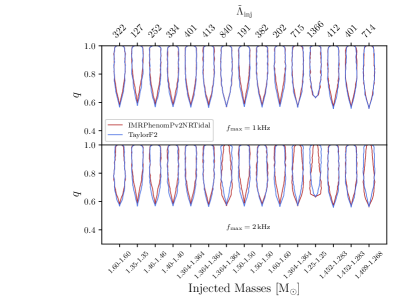
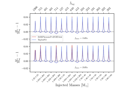
Figure 4: Distributions of the mass ratio $q$ (top) and the deviation from the injected total mass $M_{\rm inj}$ (bottom), displayed for all the simulated signals of Table 1. The distributions recovered are consistent between different approximants and frequency ranges. The unequal mass signals cannot be distinguished from their equal mass counterpart.

IV.2 Masses, mass-ratio and spins

We first discuss the determination of the nontidal parameters. Figure 4 shows the recovered posterior distributions of the total mass $M$ and mass ratio $q$ parameters obtained with low spin priors. The estimates obtained are consistent between the different approximants, frequency cutoffs and with the injected signals, with the real values always falling inside the $90\%$ credible intervals. This indicates that the systematic differences in phasing observed at low frequencies (see the first column of Fig. 2) are smaller than statistical uncertainties. We find that the injected unequal-mass signals (with $q=0.86$ and $q=0.88$) cannot be distinguished from the equal mass ones. This can partly be attributed to the known existing correlation between mass ratio and spin parameters Cutler and Flanagan (1994). In PN waveforms the leading order spin interactions are described by the parameter $\beta$, given by Cutler and Flanagan (1994); Arun et al. (2009)

$$\beta=\chi_{\rm eff}-\frac{38\nu}{113}(\chi_{1}+\chi_{2}),$$ (28)

where

$$\chi_{\rm eff}=\frac{m_{1}\bm{\chi}_{1}+m_{2}\bm{\chi}_{2}}{M}\cdot\bm{\hat{L}}$$ (29)

is the mass weighted sum of the component spin parameters, and is often times used during PE as a measure of the collective spin of the binary, as it is a conserved quantity of the orbit-averaged precession equations over precession timescales Racine (2008). A Fisher Matrix analysis reveals that spin parameters, which at leading order have $p=-4$ in the notation of Sec. II, are measured over a very similar range of frequencies as the (symmetric) mass ratio $\nu$ Damour et al. (2012); Harry and Hinderer (2018), to which they are therefore strongly correlated. In more detail, positive aligned spins have a repulsive effect on the binary dynamics. By contrast, decreasing the symmetric mass ratios (i.e, more unequal-mass systems) accelerates the coalescence. The two effects are thus in direct competition, and spin effects can be reproduced by varying $\nu$ Baird et al. (2013). As a consequence, widening the spin-priors leads to larger mass ratio distributions. Hence, different prior assumptions on mass ratio and component spins can lead to very different posterior distributions, and are of key importance when interpreting the data. In Appendix A, from Eq. (37), we see that this correlation may also reflect on the estimate of $\tilde{\Lambda}$ even in the case of high SNR signals, leading to an overall broadening of the $\tilde{\Lambda}$ posteriors.

IV.3 Tidal parameter and NS Radius

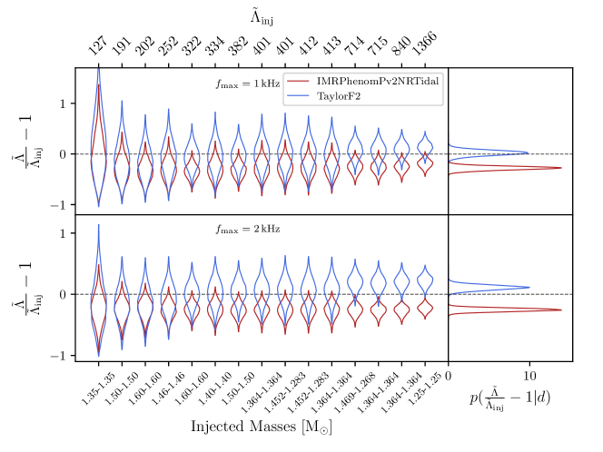
Figure 5: Main panel: violin plots of the fractional deviation between the injected values of $\tilde{\Lambda}$ and the recovered posteriors. The color code depends on the approximant employed for the PE (red for ${\tt IMRPhenomPv2NRTidal}$, blue for ${\tt TaylorF2}$), and the results are displayed for two different frequency cutoffs $f_{\rm max}$, $1$kHz (top) and $2$kHz (bottom). As matter effects grow, the deviation between the two approximants and the TEOBResumS baseline increases, reaching approximately $\pm 20\%$ when $\tilde{\Lambda}^{\rm inj}=1366$. On the right panel, we display the combined posterior distribution of the fractional deviation reweighted as described in the text. An increase of $f_{\rm max}$ negatively impacts the overall differences in the recovery of $\tilde{\Lambda}$ between models. This is especially true for ${\tt TaylorF2}$: PN waveform models are known to become less accurate close to merger frequencies.

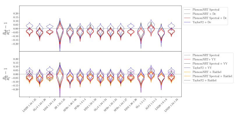
Figure 6: Fractional deviation between the real ”injected” values $R_{\rm inj}$, computed for each signal listed in Table 1, and the distributions of $R$ computed either using the universal relations of Table 2 (colored lines) or by considering the parameterized EOS posteriors and solving the NS structure equations (black lines). Whenever posteriors from the parameterized EOS (”spectral”) runs are involved, we employ straight lines. Conversely, whenever we use posteriors from analyses performed by sampling $\Lambda_{A}$ and $\Lambda_{B}$ independently we use dashed lines. The under/over estimates displayed by ${\tt IMRPhenomPv2NRTidal}$ and ${\tt TaylorF2}$ in Figure 5 translate into similar biases on $R$, amounting up to $\pm 5\%$.

Table 2: Summary of the the quasi-universal relations used in Sec. IV.3. While the De et al. (De) relation immediately links the radius of a $1.4{\rm M_{\odot}}$ NS to the mass-weighted tidal deformability and chirp mass of a BNS system, The Yagi-Yunes (YY) and Raithel et al. (R) relations require the numerical inversion of $\tilde{\Lambda}(R,q)$. For more detail, see Appendix D

Shorthands	References	Expressions
De (De et al.)	De et al. (2018)	Eq. (39)
YY (Yagi and Yunes)	Yagi and Yunes (2016, 2017)	Eq. (40), (42)
R (Raithel et. al)	Raithel (2019)	Eq. (43)

We now discuss systematics in the inference on tidal parameters and the effect on constraints on the NS radius. Figure 5 shows the posterior distributions of the tidal parameters $\tilde{\Lambda}$ recovered through PN and Phenomenological approximants. The values coming from the posterior samples are re-scaled by the true injected value, adopting the auxiliary parameter

$$\varepsilon_{\tilde{\Lambda}}^{(i)}=\frac{\tilde{\Lambda}^{(i)}}{\tilde{\Lambda}_{\rm inj}^{(i)}}-1\ ,$$ (30)

which encodes the fractional deviation from the injected value for each simulated signal $i$. We observe that, as the injected values of $\tilde{\Lambda}$ increase, the relative uncertainties of the recovered posterior distributions decrease and modeling differences become more relevant (the median of the distributions are shifted with respect to zero). The combination of these two effects leads to evident biases in the recovered values. The overall bias due to waveform effects is quantified by the combined posterior distribution $p(\varepsilon_{\tilde{\Lambda}}|d)$ shown in the right panel of Fig. 5. This quantity is estimated weighting each posterior distribution $p(\varepsilon_{\tilde{\Lambda}}^{(i)}|d)$ by the respective prior distribution $p(\varepsilon_{\tilde{\Lambda}}^{(i)})$, computed from the prior distributions for $\tilde{\Lambda}^{(i)}$. The result is multiplied by the prior distribution $p(\varepsilon_{\tilde{\Lambda}})$ for the combined parameter $\varepsilon_{\tilde{\Lambda}}$, taken as uniform in the range $[-2,+2]$, i.e.

$$p(\varepsilon_{\tilde{\Lambda}}|d)=p(\varepsilon_{\tilde{\Lambda}})\prod_{i}\frac{p\Big{(}\varepsilon_{\tilde{\Lambda}}^{(i)}\Big{|}d\Big{)}}{p\Big{(}\varepsilon_{\tilde{\Lambda}}^{(i)}\Big{)}}\,,$$ (31)

where the index $i$ runs over all the injected binaries. We find that IMRPhenomPv2NRTidal systematically recovers lower values than those injected with TEOBResumS, while TaylorF2 tends to systematically overestimate tidal parameters as matter effects increase, although it is able to capture the injected values for $\tilde{\Lambda}\leq 400$. These results can be understood in terms of the $Q_{\omega}$ analysis of Sec. III, coupled to the relevant frequency ranges computed and discussed in Appendix B. To summarize, the analyzed signals contain useful information up to approximately 1kHz, depending on the source parameters. We are then consistently in the situation where $f_{\rm thr}$ is larger than $f^{\tilde{\Lambda}}_{5\%}$, whose values lie around $240-300$ Hz. Then, as shown in the third column of figure 2, for IMRPhenomPv2NRTidal systematical differences in $\tilde{\Lambda}$ are dominated by the tidal sector, which is more attractive than TEOBResumS and leads to lower estimates of $\tilde{\Lambda}$. The attractive point mass contribution of TaylorF2, instead, leads to slight underestimates of the tidal parameters for values of $\tilde{\Lambda}\approx 100$, while for $\tilde{\Lambda}\approx 400$ it compensates the tidal sector. The latter dominates for larger values of $\tilde{\Lambda}$, and – being too repulsive – causes overestimates of matter effects.

Translating information on the tidal parameters of a NS into information on the NS EOS and radius is not straightforward. Given that waveform models do not explicitly depend on the NS radius, it is not possible to directly extract $R$ from GW data. It is necessary, instead, to rely on either some parameterization of the EOS Read et al. (2009); Raaijmakers et al. (2018); Lindblom (2010); Lindblom and Indik (2014), or on quasi-universal (EOS-insensitive) relations, which phenomenologically link macroscopic quantities of the binary between each others. In particular, we employ the spectral parameterization of Lindblom (2010); Lindblom and Indik (2014) and the EOS universal relations of De and Lattimer De et al. (2018), of Raithel et al Raithel (2019), and of Yagi and Yunes Yagi and Yunes (2016, 2017). The EOS-insensitve relations used here are summarized in Appendix D.

In the reminder of this subsection we focus on the implication of waveform systematics on the recovery of the NS radii and EOS reconstruction. We additionally gauge the further biases that can be introduced by employing quasi-universal relations for the recovery of $R$. To do so, we apply the above UR to the analyses performed by sampling the component tidal parameters $\Lambda_{i}$ independently of each others, as well as to (spectral) parameterized EOS runs. Indeed, the parameterized posterior EOS obtained are usually employed in conjunction with the component mass posteriors $m_{i}$ to solve the TOV structure equations, and obtain a direct estimate of $R$. At the same time, however, given an EOS and the component masses, it is possible to compute $\tilde{\Lambda}$, apply some UR and obtain another – in principle equivalent – estimate of $R$. This allows for a direct comparison of the effects of using universal relations in place of parameterized EOS runs, independently of the choice of the sampling parameters (and, therefore, of the implied priors on $\tilde{\Lambda}$). Figure 6 shows the distributions of the deviation in the estimates of $R_{1.4{\rm M_{\odot}}}$ (top panel) and $R_{2}$ (bottom panel) with respect to the real radii values corresponding to the parameters and EOSs listed in Table 1. We find that IMRPhenomPv2NRtidal tends to underestimate $R$, while TaylorF2 behaves in the opposite way. The overall bias can amount up to approximately $\pm 5\%$ between TEOBResumS and PN/phenomenological waveforms and $10\%$ between ${\tt IMRPhenomPv2NRTidal}$ and ${\tt TaylorF2}$. Mirroring the behavior of $\tilde{\Lambda}$, it becomes more relevant as tidal effects grow. Additionally, all universal relations lead to slight underestimates of the values of R with respect to the ones recovered from spectral runs. We find that the true values of $R$ fall outside the $90\%$ credible intervals in a significant number of cases, especially when computing $R_{1.4{\rm M_{\odot}}}$. In our situation, with an injected EOB waveform, we find that while this additional difference impacts negatively IMRPhenomPv2NRTidal analyses, TaylorF2 runs would gain from using universal relations rather than a parameterized analysis.

IV.4 Faithfulness thresholds and PE biases

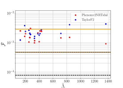
Figure 7: Unfaithfulness values between the IMRPhenomPv2NRTidal (red) or TaylorF2 (blue) waveforms and the injected TEOBResumS waveforms. The plus and cross polarizations are projected on to the Livingston detector, and the source is fixed at the GW170817 sky location. Horizontal straight lines correspond to the treshold values of $\bar{\mathcal{F}}$ obtained with an SNR of $80$ (black) and $32.4$ (orange), computed through Eq. 19 with $\epsilon=6$ (straight) and $\epsilon=1$ (dashed). Dots correspond to waveforms with $q=1$, while diamonds to signals with $q\neq 1$.

Finally, we apply the accuracy criteria of Sec. II to our data and show that, while criteria based on faithfulness alone are of little use to predict the presence of biases, an estimate of the parameter bias can be obtained using Eq. (24). We begin by computing the unfaithfulness $\bar{\mathcal{F}}$ between waveform models evaluated with the same set of true parameters $\theta_{\text{inj}}$ through Eq. (5). We place all sources in GW170817’s sky location, and employ the analytical aLIGODesignSensitivityP1200087 PSD Aasi et al. (2015), provided by pycbc Nitz et al. (2020). The results are summarized in Fig. 7. We find that both TaylorF2 and IMRPhenomPv2NRTidal give values largely above the nominal threshold of $\bar{\mathcal{F}}=0.03$ (not shown in figure), which corresponds to ${\sim}10$% of detection losses Cutler and Flanagan (1994); Lindblom et al. (2008). When considering the thresholds provided by Eq. 19 in its weaker formulation ($\epsilon^{2}=6$), we find that most signals fall above the value corresponding to GW170817’s network SNR (straight orange line), and largely below the threshold corresponding to a network ${\rm SNR}$ or $80$ (straight black line), i.e the SNR above which all of our injections are performed. By tightening the constraints and enforcing $\epsilon^{2}=1$ (dashed lines), we find that already at the SNR of GW170817 none of the considered signals are faithful enough to ensure that no waveform systematics will be observed. However, not all our injections give largely biased or uncompatible results. These facts remark that these criteria give necessary but not sufficient rules to identify biases and highlight the strong dependence of the criteria themselves on the arbitrarily chosen value of $\epsilon^{2}$.

To obtain an estimate of the biased values $\tilde{\Lambda}_{E}$ we apply Eq. (24), and minimize the quantity $\sum_{i}(h^{{\tt TEOBResumS}}_{i}-h^{{\tt IMRPhenomPv2NRTidal},{\tt TaylorF2}}_{i}|h^{{\tt TEOBResumS}}_{i}-h^{{\tt IMRPhenomPv2NRTidal},{\tt TaylorF2}}_{i})$, where the sum is performed over the network interferometers considered (Livingston, Hanford and Virgo, in our case). In particular, for each waveform $h^{{\tt IMRPhenomPv2NRTidal},{\tt TaylorF2}}$ we fix the intrinsic parameters $(m_{A},m_{B},\chi_{A},\chi_{B})$ to their real injected values, and vary $\Lambda_{A}=\Lambda_{B}$ over the one-dimensional interval $\tilde{\Lambda}\in[\min(0,\tilde{\Lambda}_{\rm inj}-500),\tilde{\Lambda}_{\rm inj}+500]$. The simplifying choice of imposing $\Lambda_{A}=\Lambda_{B}$ can be justified by considering that in our injection study we were unable to distinguish $q=1$ from $q\neq 1$ systems. While this might not be true for more asymmetric systems than those studied in the present paper, the issue can be easily circumvented by employing Binary-Love universal relations Yagi and Yunes (2016). The straightforward procedure described leads to the values displayed in Table 1. We find that the $\tilde{\Lambda}_{E}$ values computed, while often slightly overestimated with respect to the medians of the distributions of the tidal parameters recovered through PE, fall into the $90\%$ $\tilde{\Lambda}$ credible limits in the large majority of cases, thus providing a good approximation of the overall behavior of the approximants employed. Due to the overestimate of $\tilde{\Lambda}_{E}$, the bias $\Delta\tilde{\Lambda}_{B}=|\tilde{\Lambda}_{E}-\tilde{\Lambda}_{\rm inj}|$ is larger than the real bias $\Delta\tilde{\Lambda}_{\rm true}=|\tilde{\Lambda}^{\rm median}-\tilde{\Lambda}_{\rm inj}|$ for the TaylorF2 approximant, and smaller for IMRPhenomPv2NRTidal. Estimates of waveform systematics based on the above method might then be slightly optimistic (pessimistic) when comparing TEOBResumS to IMRPhenomPv2NRTidal (${\tt TaylorF2}$).

V GW170817

We now apply the approach developed and tested in the previous sections to the analysis of GW170817.

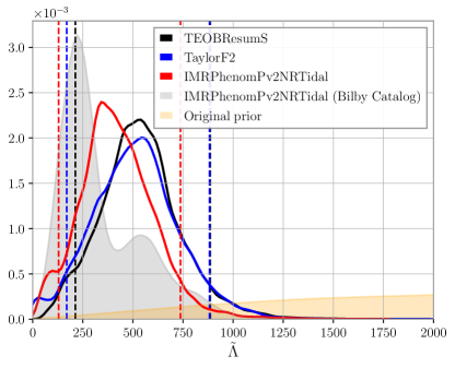
Figure 8: Analysis of GW170817 data. Marginalized one-dimensional $\tilde{\Lambda}$ posteriors, obtained analyzing the data up to $f_{\rm max}=1024$ Hz with three approximants: ${\tt TaylorF2}$ (blue), ${\tt IMRPhenomPv2NRTidal}$ (red) and ${\tt TEOBResumS}$ (black). The posteriors shown are reweighted to flat in $\tilde{\Lambda}$ prior, as is done in e.g Abbott et al. (2019a). The public bilby posteriors from Ref. Romero-Shaw et al. (2020) (grey) are also displayed. Note that the bilby analysis uses $f_{\rm max}=2048$ Hz.

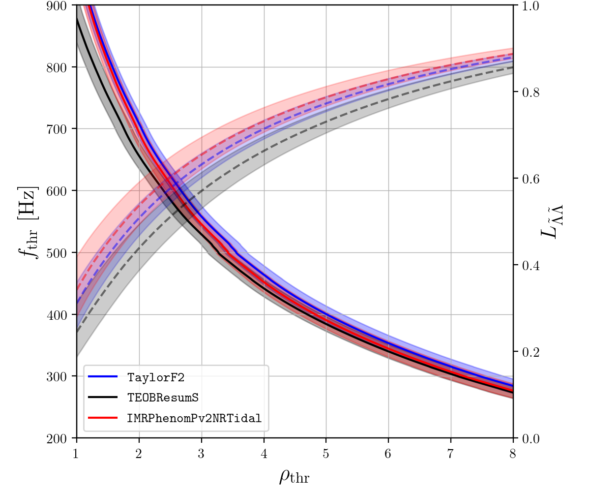
Figure 9: Estimation of $f_{\rm thr}$ (solid lines) and $L_{\tilde{\Lambda}\tilde{\Lambda}}$ (dashed lines) from GW170817 posterior samples extracted with ${\tt TaylorF2}$ (blue), ${\tt IMRPhenomPv2NRTidal}$ (red) and ${\tt TEOBResumS}$ (black). The shadowed bands represent the 90% credible regions. In order to evaluate $f_{\rm thr}$, we use the identical waveform models involved in the extraction of the posterior samples and we set an cut-off frequency at merger $f_{\rm mrg}$, estimated with the fits introduced in Ref. Breschi et al. (2019). For the estimation of $L_{\tilde{\Lambda}\tilde{\Lambda}}$, we limit ourselves to $6.5{\rm PN}$ phase corrections. The plotted values are computed using a network of three detectors (two LIGOs and Virgo) and setting $f_{\rm max}=2~{}{\rm kHz}$. For a single interferometer at $\rho_{\rm thr}=1$, we get $f_{\rm thr}\approx 700~{}{\rm Hz}$ for LIGO’s detectors and $f_{\rm thr}\approx 250~{}{\rm Hz}$ for Virgo.

We perform a Bayesian analysis of GW170817 using the ${\tt IMRPhenomPv2NRTidal}$, ${\tt TaylorF2}$ and ${\tt TEOBResumS}$ approximants, involving pbilby Smith and Ashton (2019). We adopt an almost identical configuration to the one presented in Ref. Romero-Shaw et al. (2020) (see also Abbott et al. (2019a)). In more detail, we consider a strain of 128 s around the GPS time $1187008882.43$ s. Data is downloaded directly from the GWOSC Abbott et al. (2019b), in its cleaned and deglitched version (v2). We employ the PSDs provided by Abbott et al. (2019a), and fix the sky location to the one provided by EM constraints. Further, as we are mainly interested estimating the intrinsic parameters of the source, we marginalize over distance, time and phase. The sampling is performed with uniform priors in chirp mass $\mathcal{M}\in[1.18,1.21]{\rm M_{\odot}}$ and mass ratio $q\in[0.125,1]$, with the additional constraints $m_{A},m_{B}\in[1.001398,4.313897948277728]{\rm M_{\odot}}$. The quadrupolar tidal coefficients $\Lambda_{A},\Lambda_{B}$ are uniformly sampled in the interval $[0,5000]$. The main differences w.r.t the analysis of Ref. Romero-Shaw et al. (2020) lie in (i) the different spin priors employed, which are taken to be aligned to the orbital angular momentum and such that $(\chi_{A},\chi_{B})\in[-0.05,0.05]$, and (ii) in the high-frequency cutoff of 1024 Hz that we impose (instead of the 2048 Hz of Romero-Shaw et al. (2020)).

Using the formalism of the Fisher matrix outlined in Sec. II.1, we investigate in which frequency region the tidal information is effectively extracted, according with the extracted posterior samples: the Fisher’s matrix element $I_{\tilde{\Lambda}\tilde{\Lambda}}$ has its main support in the frequency band from $200~{}{\rm Hz}$ to $1.5~{}{\rm kHz}$. Subsequently, we compute $f_{\rm thr}$ according to Eq. (15) and, in order to achieve a more realistic result, we neglect the contributions above merger frequency $f_{\rm mrg}$, where this quantity is estimated using numerical relativity fits introduced in Ref. Breschi et al. (2019). As shown in Fig. 9, we find that the SNR of GW170817 is located at frequencies lower than ${\sim}700$ Hz (depending on the chosen value of $\rho_{\rm thr}$). More precisely, we can say that the signal power enclosed above ${\sim}900~{}{\rm Hz}$ does not exceed an SNR of 1 (which roughly corresponds to 3% of the total SNR), while the power above ${\sim}550~{}{\rm Hz}$ cannot contribute more than an SNR of 3 (10% of the total SNR). The large variability of $f_{\rm thr}$ with the chosen value of $\rho_{\rm thr}$ indicates that a relatively small fraction of the SNR is accumulated over a rather large frequency interval. The estimation of $f_{\rm thr}$ motivates our choice of $f_{\rm max}=1~{}{\rm kHz}$: indeed, we do not expect to find a relevant portion of signal above this limit. Furthermore, this upper bound minimizes errors due to possible high-frequency noise fluctuations. From the discussion of Sec. II, one expects the masses of the binary to be measured rather accurately. The reduced tidal parameter, instead, will be affected by significant statistical uncertainties: from the posterior samples, we estimate a loss of tidal information of $L_{\tilde{\Lambda}\tilde{\Lambda}}\sim 20-50\%$, for $\rho_{\rm thr}\sim 1-3$.

The marginalized tidal parameter posteriors reweighted to flat in $\tilde{\Lambda}$ prior are shown in Fig. 8. All the measurements agree within 95% confidence region, thus indicating that waveform systematics are not the main source of uncertainty. However, the distributions for the different approximants do suggest the presence of some systematic effects. These posteriors should be interpreted in terms of the phasing plots in Fig. 2 for $f\lesssim 700\,$kHz (low frequency part of right panel) and $\tilde{\Lambda}\lesssim 1000$. The phasing analysis of Sec. III shows that ${\tt IMRPhenomPv2NRTidal}$ is more attractive than ${\tt TEOBResumS}$ and ${\tt TaylorF2}$; the systematic differences in the relevant frequency regime are dominated by the tidal part (${\tt IMRPhenomPv2NRTidal}$ vs others) or by a mixture of the point-mass and tides (${\tt TaylorF2}$ vs ${\tt TEOBResumS}$). This is consistent with the slightly smaller $\tilde{\Lambda}$ measured with the ${\tt IMRPhenomPv2NRTidal}$ with respect to the other approximants and attributable to the particular design of ${\tt IMRPhenomPv2NRTidal}$ (PN tides at LO in the low frequency regime, ${\tt TEOBResumS}$ in middle regime frequency and NR data at higher frequencies; with LO tides stronger than PN NLO, NNLO, and EOB tides at low frequencies, and NR tides typically stronger than EOB tides Bernuzzi et al. (2012a, 2015b)). ${\tt TEOBResumS}$ measurement is instead compatible with ${\tt TaylorF2}$. This is again understandable from the phasing plots discussed in Sec. III: for $\hat{\omega}\sim 0.035-0.06$, the differences in the point-mass and tidal sector between the approximants have opposite sign and partially compensate each other. Nonetheless, it is not possible from this analysis to identify whether a model is preferred by the data available, consistently with the conclusion of Abbott et al. (2017a, 2019c). We report in Table 3 the evidences given by the different approximants. We conclude that systematics effects are observable in GW170817, but do not dominate the measurement of $\tilde{\Lambda}$. These effects are nonetheless expected a priori from the phasing analysis of Sec. III.

Note that our ${\tt IMRPhenomPv2NRTidal}$ posteriors do not present the double-peak in $\tilde{\Lambda}$ that is instead found in Abbott et al. (2017a, 2019c). The reason for this difference lies in the high-frequency cutoff imposed. This same effect had already been noticed in Ref. Dai et al. (2018). The authors, using the spin-aligned IMRPhenomDNRTidal model Husa et al. (2016); Khan et al. (2016) to analyze the data, together with the relative binning technique Zackay et al. (2018), found a double-peak structure in the posterior of $\tilde{\Lambda}$ with $f_{\rm max}=1.5$ kHz, that however disappeared when $f_{\rm max}$ was lowered to 1 kHz. Repeating our analysis with ${\tt IMRPhenomPv2NRTidal}$ and $f_{\rm max}=2$ kHz, we too re-obtain the double peak in $\tilde{\Lambda}$. The evidence of the newer analysis is, however, compatible to the one reported in Table 3: $\ln p(d|{\tt IMRPhenomPv2NRTidal},2{\rm kHz})=$ 521.860 $\pm$ 0.103. This implies that negligible SNR is accumulated above 1 kHz, and that the double peak is not to be interpreted as a physically motivated feature of the posteriors, but rather can be attributed to some high frequency noise fluctuation. This fact is also supported by the estimation of $f_{\rm thr}$.

Overall, we find consistent values for intrinsic parameters such as masses and spins with Abbott et al. (2017a, 2019c) and higher $\tilde{\Lambda}$ values. To translate the information on $\tilde{\Lambda}$ to constraints on the NS radius $R$ we apply the UR of De et al. (2018) to the reweighted ${\tt TEOBResumS}$ $\tilde{\Lambda}$ posteriors and estimate the radius of a $1.4{\rm M_{\odot}}$ NS. We find $R_{1.4}=12.5^{+1.1}_{-1.8}$ km. This value is slightly larger – though still compatible – than the one obtained in Abbott et al. (2017a). The effect of the key choices of our analysis, i.e the high frequency cutoff employed, the use of ${\tt TEOBResumS}$ and the low-spin priors imposed, is then that of pushing towards higher $R$ values and softer EOSs. In the literature, additional radius estimates have been computed by including further astrophysical information. We find our result, which focuses on the implications of GW data alone, to be in good agreement with the radii obtained when additionally accounting for electromagnetic-priors Radice and Dai (2019) and the measurement given by NICER. Raaijmakers et al. (2019, 2020), which too favour $\tilde{\Lambda}$ values larger than $\approx 200$.

Table 3: Analysis of GW170817 data: log-evidences and corresponding standard deviations computed using different waveform approximants: ${\tt TEOBResumS}$, ${\tt TaylorF2}$ and ${\tt IMRPhenomPv2NRTidal}$. The values obtained, according to standard Bayesian statistics, indicate that it is not possible to identify a preferred waveform model exclusively by relying on the GW170817 data.

Approximant	$\ln p(d|{\rm Approx.})$
${\tt TaylorF2}$	$523.078\pm 0.102$
${\tt TEOBResumS}$	$522.585\pm 0.102$
${\tt IMRPhenomPv2NRTidal}$	$522.261\pm 0.103$

VI Tides inference with 3G detectors

Third generation detectors such as Einstein Telescope Sathyaprakash et al. (2011); Maggiore et al. (2020) and Cosmic Explorer Reitze et al. (2019) are expected to start taking data in the late 2020s. Their increased sensitivity at high frequencies will significantly improve the detection of tidal signatures in the inspiral, and even allow the detection of GWs from the remnant. Typical SNRs expected for GW170817-like events detected by ET are of the order of 1700. As a consequence, the importance of waveform systematics is expected to further increase with respect to second generation detectors.

To summarize some the arguments of Sec. II, the SNR enters the determination of $\tilde{\Lambda}$ through two main channels. Firstly, it determines the maximum useful frequency $f_{\rm thr}$ (see Eq. (15)), above which variations of $\rho$ can be fully attributed to statistical fluctuations and which determines the regimes at which tidal measurements are performed. Secondly it is related to the width of the distribution of the tidal parameter $\sigma_{\tilde{\Lambda}}=\tilde{\Lambda}^{95^{\rm th}\%ile}-\tilde{\Lambda}^{5^{\rm th}\%ile}$. If the signal is loud enough – as is expected with ET and CE – $f_{\rm thr}$ will be above merger frequency for a large fraction of events. Therefore, when studying the signal with inspiral-merger only waveform models, the effect of varying the SNR will mainly affect $\sigma_{\tilde{\Lambda}}$. To obtain a quantitative estimate of $\sigma_{\tilde{\Lambda}}$ for 3G detectors we fit the values found in our injection study and extrapolate them to higher SNRs. We find that a good approximation of the behavior of $\sigma_{\tilde{\Lambda}}$ over the SNR range we considered is obtained by assuming that

$$\sigma_{\tilde{\Lambda}}(\rho)=\frac{c}{\rho-\rho_{0}}.$$ (32)

This functional form is valid only for $\rho>\rho_{0}$, in which case the denominator can be expanded as a geometrical series, and incorporates the corrections to the leading order $1/\rho$ asymptotical behavior expected from the Fisher Matrix analysis. Fitting Eq.(32) to the data we find $(c,\rho_{0})=(7497.965751,63.092154)$ for TaylorF2 and $(4372.214662,66.778801)$ for IMRPhenomPv2. As could already be observed from Fig. 5, ${\tt IMRPhenomPv2NRTidal}$ constrains the tidal parameter better than its PN counterpart: $\sigma_{\tilde{\Lambda}}^{\rm Phenom}(\rho)$ is (almost) parallel to $\sigma_{\tilde{\Lambda}}^{\rm TaylorF2}(\rho)$ but shifted to lower values. To obtain a unique estimate of $\sigma_{\tilde{\Lambda}}$ we compute the mean value $\bar{\sigma}_{\tilde{\Lambda}}=(\sigma_{\tilde{\Lambda}}^{\rm Phenom}+\sigma_{\tilde{\Lambda}}^{\rm TaylorF2})/2$.

The expression of $\bar{\sigma}_{\tilde{\Lambda}}$ can then be used to compute the SNR at which two independent measurements $\tilde{\Lambda}_{1}$ and $\tilde{\Lambda}_{2}$, whose difference we denote as $\Delta\tilde{\Lambda}$, become statistically inconsistent. Figure 10 shows the quantity $\Delta\tilde{\Lambda}/\bar{\sigma}_{\tilde{\Lambda}}$ as a function of the optimal SNR $\rho$ for values of $\Delta\tilde{\Lambda}\in[-100,100]$. When $\Delta\Lambda/\bar{\sigma}_{\tilde{\Lambda}}\approx 1$, statistical fluctuations are of the same order of magnitude as systematical effects. For $|\Delta\tilde{\Lambda}|\approx 100$, we see that this condition is satisfied already at the threshold $\rho\approx 125$. As $|\Delta\tilde{\Lambda}|$ decreases, the threshold SNR increases, reaching $\rho\approx 300$ in correspondence of a $\Delta\tilde{\Lambda}\approx 20$.

The above considerations are independent of the exact waveform models employed, and do not tackle the issue of estimating the $\Delta\tilde{\Lambda}$ associated to two specific chosen approximants. While it is clear from the injection study of Sec. IV that large $\Delta\tilde{\Lambda}$ are to be expected when employing ${\tt TaylorF2}$ and ${\tt IMRPhenomPv2NRTidal}$, we take a step further and qualitatively estimate the bias $\Delta\tilde{\Lambda}=\tilde{\Lambda}_{E}-\tilde{\Lambda}$ through Eq. (24) for two additional state-of-the-art approximants, IMRPhenomPv2NRTidalv2 Dietrich et al. (2019) and SEOBNRv4Tsurrogate Lackey et al. (2018). We thus compare the latter and TEOBResumS in pairs and report the differences with respect to two baselines (TEOBResumS and SEOBNRv4Tsurrogate). Following the procedure described in Sec. IV.4 we consider values of $\tilde{\Lambda}$ equal to $400$, $800$ and $1000$, place the sources in GW170817’s location and employ the EinsteinTelescopeP1600143 PSD Abbott et al. (2017c). We compute waveforms from $30$ to $2048$ Hz (left panel) or $1024$ Hz (right panel). Results are again displayed in Fig. 10.

We find that both SEOBNRv4Tsurrogate and IMRPhenomPv2NRTidalv2 “underestimate” the values of $\tilde{\Lambda}$ of the TEOBResumS baseline (right panel), and that the $|\Delta\Lambda|$ found are always below $\approx 100$. This indicates that tides are stronger in the SEOBNRv4Tsurrogate and IMRPhenomPv2NRTidalv2 models than in TEOBResumS. When restricting below 1kHz (large $\tilde{\Lambda}$) the systematic bias in $\tilde{\Lambda}$ due to the differences between IMRPhenomPv2NRTidalV2 and TEOBResumS is ${\lesssim}2\sigma$ corresponding to $\Delta\tilde{\Lambda}\pm 50$, while it varies ${\sim}2-4\sigma$ when considering differences with respect to SEOBNRv4Tsurrogate. This indicates that the differences between IMRPhenomPv2NRTidalv2 and TEOBResumS are mostly related to the modeling of tides at high-frequencies, while the tides in the EOB models differ from each other already at lower frequencies.

Some caution is needed when interpreting the results obtained for the different waveform approximants: in Sec. IV.4 we have seen that at times the estimated $\tilde{\Lambda}_{E}$ would overestimate $\tilde{\Lambda}^{\rm median}$ by up to $100$. This difference was acceptable at the injected SNRs, but indicates that our estimate might not precise enough at the SNRs which characterize 3G detectors. Nonetheless, we expect the behavior of the approximants (i.e, their being more/less attractive) to be correctly captured.

Overall, our findings indicate that above SNR $\approx 100-200$ $\sigma_{\tilde{\Lambda}}$ will be small enough that the models will appear to be fully inconsistent between each others. The estimated systematic biases reflect differences in the tidal modeling at frequencies corresponding to the very last orbits and thus accessible to NR. We stress that at frequencies $\hat{\omega}_{22}\gtrsim 0.06$ the NS are in contact and the waveform modeling based on tidal interactions can only be considered an effective description, since the dynamics is dominated by hydrodynamics Bernuzzi et al. (2012a). We demonstrate in Appendix C that current NR simulations are not sufficiently accurate to produce faithful waveforms. New, more precise NR simulations appear crucial to further develop tidal waveform models for future detectors.

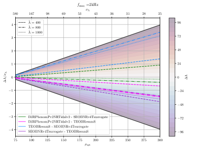
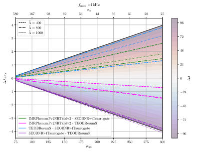
Figure 10: The ratio between systematic effects $\Delta\tilde{\Lambda}$ and statistical uncertainties $\sigma_{\tilde{\Lambda}}$, shown as a function of the SNR $\rho$ for a range of different $\Delta\tilde{\Lambda}\in[-100,+100]$. Colored lines refer to values of $\Delta\tilde{\Lambda}/\sigma_{\tilde{\Lambda}}$ estimated between a baseline approximant Y and a recovery approximant X, labelled as “X-Y” in the bottom-left legend, and computed for two different frequency cutoffs (left and right panels) and three different values of $\tilde{\Lambda}$ (dashed, dotted and dash-dotted lines). We find that $\Delta\tilde{\Lambda}/\sigma_{\tilde{\Lambda}}\approx 1$ at SNRs ranging from 175-200 for all $\tilde{\Lambda}$ values. Therefore, with 3G detectors, all the current approximants will appear to be statistically inconsistent.

VII Conclusions

In this paper we discussed a possible approach for the analysis of waveform systematics in the estimation of tidal effects in BNS. We demonstrated the effectiveness of our method in a mock experiment using a large set of injected signals and applied the method to GW170817. We recommend to use this method for future analysis and point out that the approximants used for the main analysis of GW170817 should be significantly improved for future robust analysis at SNR ${\sim}80$ and beyond. We expand on these conclusions here below.

The bottom-up method employed in this work is composed of three steps. First, the waveform approximants should be compared using the $Q_{\omega}$ analysis in order to understand the effect of the modeling choices (and the physics implemented in the models) on the GW phase. The $Q_{\omega}$ diagnostic is key to determine the waveforms’ differences and it is free from the ambiguities introduced in the phase comparisons by the time/phase shift. Second, it is important to identify what is the frequency regime at which the tidal information is effectively extracted. This can be accomplished by computing fractional losses $L_{ii}$ defined in Sec. II. Third, the PE results should be interpreted in terms of the $\Delta Q_{\omega}$ analysis on the relevant frequency interval.

Our mock experiments show that this procedure is effective in identifying the main baiases introduced by the waveform models. Note in this respect that the “target” model used for the computation of the $\Delta Q_{\omega}$ should be chosen amongst those that are considered sufficiently faithful on the relevant frequency regime. For example, for analyzing biases at low frequencies, the target model should contain maximal analytical information (vs minimal fitting), high-order Taylor or EOB models represent the best choice in this respect. At very high frequencies, numerical relativity data would be the best choice, although the accuracy of the data is not yet sufficient for robust statements (See Appendix C).

The analysis of GW170817 shows that the measurement of the tides is essentially free of systematic effects if performed up to $1\,$kHz Radice and Dai (2019); Dai et al. (2018). Extending the analysis to higher frequencies introduces some waveform effects, albeit still compatible with others in the 90% confidence region. In particular, comparing our results to Fig. 9 of Abbott et al. (2019a), we observe a shift in the posterior of $\tilde{\Lambda}$ computed with ${\tt IMRPhenomPv2NRTidal}$ that can be fully understood from the $Q_{\omega}$ phasing analysis presented here. When applying ${\tt IMRPhenomPv2NRTidal}$ to $2\,$kHz, the posteriors have a double peak that is not present with the $1\,$kHz cutoff. The similar inferences using the ${\tt TaylorF2}{}$ and ${\tt TEOBResumS}$ approximants are instead related to the fact that, in the relevant frequency regime, the differences between the ${\tt TaylorF2}{}$ point-mass and the tidal have opposite signs and partly compensate each other (see Fig. 2).

Applying the UR of De et al. (2018) to the $\tilde{\Lambda}$ values obtained in our GW170817 re-analysis we obtain a new measurement of $R_{1.4{\rm M_{\odot}}}$ which – based exclusively on the information gathered from GW data – is in good agreement with results coming from independent astrophysical observations, i.e the NICER radius measurement and the information coming from EM observations Radice and Dai (2019); Raaijmakers et al. (2019).

Significant waveform systematics are to be expected for GW170817-like signals already for the current advanced detectors at design sensitivity. Note these high-SNR signals are the only/best candidates for an actual measure (vs. upper limit) of the tidal parameters and EOS constraints. At design sensitivity, the expected bias in the reduced tidal parameter using ${\tt TaylorF2}$ and ${\tt IMRPhenomPv2NRTidal}$ is about $2-\sigma$ (for average BNS parameters as quantified in Fig. 5). This would reflect in systematics on the NS radius of about $1$ km (10%), that are comparable or well above of the current best estimates of the NS radius, also including electromagnetic constraints Annala et al. (2018); Abbott et al. (2018a); De et al. (2018); Radice and Dai (2019); Capano et al. (2020).

Moving to higher sensitivities and 3G detectors, we estimate that the systematics between the approximants that currently have the smallest differences among themselves become dominant over statistical errors at SNR 200 and for $\tilde{\Lambda}\gtrsim 400$ (Fig. 10). This implies that EOS constraints from the potentially most informative (and rare) events will be harmed by tidal waveform systematics.

Appendix A Effect of the point mass sector on $\tilde{\Lambda}$

In this apendix, we explicitly show how uncertainties in the point mass phase (of both statistic and systematic nature) can affect the determination of the tidal parameter $\tilde{\Lambda}$. Starting from Eq. (7), writing $\exp(i\Delta\Psi)=\cos(\Delta\Psi)+i\sin(\Delta\Psi)$, and expanding the cosine around $\Delta\Psi\approx 0$ the SNR becomes

$$\begin{split}\rho&=\frac{4}{\sqrt{(h|h)}}\int\frac{\tilde{A}_{d}\tilde{A}_{h}}{S_{n}}\left[1-\frac{(\Delta\Psi)^{2}}{2}+O\left(\Delta\Psi^{3}\right)\right]{\rm d}f\\ &\simeq\rho_{\rm opt}-\frac{2}{\sqrt{(h|h)}}\int\frac{\tilde{A}^{2}(\Delta\Psi)^{2}}{S_{n}}{\rm d}f\,,\end{split}$$ (33)

where the last step assumes $\tilde{A}_{h}\approx\tilde{A}_{d}=\tilde{A}$. By defining $\bar{\bm{\theta}}$ as the set of parameters such that $\Delta\Psi(\bar{\bm{\theta}};f)\approx 0$ over the whole frequency range considered $[f_{\rm min},f_{\rm max}]$, and expanding $\Delta\Psi$ in Eq. (33) around $\bar{\bm{\theta}}$, the second integral in Eq. (33) can be connected to the Fisher matrix

$$\int\frac{\tilde{A}^{2}(\Delta\Psi)^{2}}{S_{n}}{\rm d}f\approx\int\frac{\tilde{A}^{2}\partial_{i}\Psi_{h}\partial_{j}\Psi_{h}}{S_{n}}\Delta\theta^{i}\Delta\theta^{j}{\rm d}f$$ (34)

with $\partial_{i}=\partial/\partial\theta^{i}$ and $\Delta\theta^{i}=\theta^{i}-\bar{\theta}^{i}$ (repeated indeces imply a summation). Under the assumption of high SNR, the integrals over $f$ in Eq. (34) can be split as

$$-\frac{\Delta\theta^{l}\Delta\theta^{m}}{2}\int_{f_{\rm min}}^{f_{c}}I_{l,m}{\rm d}f-\frac{\Delta\theta^{\tilde{\Lambda}}\Delta\theta^{\tilde{\Lambda}}}{2}\int_{f_{c}}^{f_{\rm max}}I_{\tilde{\Lambda},\tilde{\Lambda}}{\rm d}f,$$ (35)

where $f_{c}$ is a “cutoff frequency” that identifies the beginning of the relevant frequency support of $I_{\tilde{\Lambda},\tilde{\Lambda}}$ (see Eq. (14)) and has the value of $\approx 300\,$Hz for fiducial BNS. Eq. (35) clearly shows the different frequency regimes at which the parameters are measured during PE. $\bar{\mathcal{M}},\bar{q}$ and $\bar{\chi}$ are determined during the early inspiral $(f\leq f_{c})$; $\bar{\tilde{\Lambda}}$ at higher frequencies $(f\geq f_{c})$. Sampling methods will tend to recover the parameters $\bm{\theta}\rightarrow\bar{\bm{\theta}}$. However, due to the varying sensitivity of the detector over different frequency ranges, the parameters measured during the early inspiral $\bm{\theta}_{\rm insp}=({\mathcal{M},q,\chi})$ converge faster than tidal parameters. Let’s then go back to Eq. (34) and express its left hand side as

$$-\frac{\Delta\theta^{l}\Delta\theta^{m}}{2}\int_{f_{\rm min}}^{f_{c}}I_{l,m}{\rm d}f-\frac{1}{2}\int_{f_{c}}^{f_{\rm max}}\frac{\tilde{A}^{2}(\Delta\Psi)^{2}}{S_{n}}{\rm d}f.$$ (36)

The first integral has, again, been expanded about the set of parameters $\bar{\theta}_{\text{insp}}$. Taking the limit $\bm{\theta}_{\rm insp}\rightarrow\bar{\bm{\theta}}_{\rm insp}$, its contribution tends to zero by definition. The remaining second integral can be explicitly written as:

$$-\frac{1}{2}\int_{f_{c}}^{f_{\rm max}}\frac{\tilde{A}^{2}}{S_{n}}\left[\Delta\Psi^{\text{PM}}(\bar{\theta}_{\text{insp}},\tilde{\Lambda}=0)+\Delta\Psi^{T}(\bar{\theta}_{\text{insp}},\tilde{\Lambda})\right]^{2}\,{\rm d}f,$$ (37)

where we have separated $\Delta\Psi$ into its point mass ($\Delta\Psi^{\rm PM}$) and tidal ($\Delta\Psi^{T}$) contributions. Critically, $\Delta\Psi^{\text{PM}}(\bar{\bm{\theta}}_{\rm insp},\tilde{\Lambda}=0)$ is not necessarily close to zero above $f_{c}$, as the parameters $\bar{\theta}_{\rm insp}$ are determined over a different regime, and chosen to minimize $\Delta\Psi^{\text{PM}}(\bar{\theta}_{\rm insp},\tilde{\Lambda}=0)$ below $f_{c}$. The value $\bar{\tilde{\Lambda}}$ therefore will have to minimize not only $\Delta\Psi^{T}$ over $[f_{c},f_{\rm max}]$, but rather the sum of $\Delta\Psi^{T}$ and $\Delta\Psi^{\text{PM}}$. This means that both the tidal and the point mass sectors of a waveform model can introduce biases in the recovery of tidal parameters, and that overall phase differences accumulated over $f_{c}$ are absorbed mainly by $\tilde{\Lambda}$.

Appendix B Tidal information

In this appendix, we apply the method presented in Sec. II.1 to the the signals involved in the PE studies of Sec. IV, proving that the injections are actually performed in an informative framework for the tidal parameter, in which statistical fluctuations cannot be considered as the dominant source of the biases observed in the tidal parameter (see Fig. 5).

Tab. 4 shows the values of the frequency support $[f_{5\%}^{\tilde{\Lambda}},f_{95\%}^{\tilde{\Lambda}}]$ defined in Eq. (14) computed for the injected signals, including all the detectors involved in the analysis. For all the cases,$f_{\rm mrg}>1~{}{\rm kHz}$, indicating the presence of signal in the high-frequency regime, and $f_{95\%}^{\tilde{\Lambda}}>1~{}{\rm kHz}$, meaning that the tidal contributions are relevant above this value. Furthermore, Tab. 4 reports the values of $f_{\rm thr}$ and $L_{\tilde{\Lambda}\tilde{\Lambda}}$, defined respectively in Eq. 15 and Eq. 16, computed for the same signals for $\rho_{\rm thr}=1,3$. For $\rho_{\rm thr}=1$, we have $f_{\rm thr}>1~{}{\rm kHz}$, showing that the signal power is relevant above this threshold. For this values, $L_{\tilde{\Lambda}\tilde{\Lambda}}\leq 30\%$. These facts are reflected in a lower variance on the posterior distribution for $\tilde{\Lambda}$ coming from the PE analyses with $f_{\rm max}=2048~{}{\rm Hz}$ with respect to the ones with $f_{\rm max}=1024~{}{\rm Hz}$. Finally, for all the injected signals, we have $f_{\rm thr}>f^{\tilde{\Lambda}}_{5\%}$, which proves that these data contains information on the tidal parameter in an accessible frequency range.

Table 4: Values of $f^{\tilde{\Lambda}}_{5\%}$, $f^{\tilde{\Lambda}}_{95\%}$, $f_{\rm thr}$ and $L_{\tilde{\Lambda}\tilde{\Lambda}}$ computed for the signals involved in the injection studies, Sec. IV. We recall that the injected signals have extrinsic properties identical to the maximum-posterior parameters of GW170817 Abbott et al. (2017a). The reported values are estimated with a three detector network (two LIGOs and Virgo) at design sensitivity using ${\tt TEOBResumS}$ waveform model.

EOS	$M$	$q$	$f_{\rm mrg}$	$f_{5\%}^{\tilde{\Lambda}}$	$f_{95\%}^{\tilde{\Lambda}}$	$\rho_{\rm thr}=1$		$\rho_{\rm thr}=3$
	[${\rm M_{\odot}}$]		[Hz]	[Hz]	[Hz]	$f_{\rm thr}$ [Hz]	$L_{\tilde{\Lambda}\tilde{\Lambda}}$	$f_{\rm thr}$ [Hz]	$L_{\tilde{\Lambda}\tilde{\Lambda}}$
DD2	2.71	1.00	1287	245	1460	1085	0.18	731	0.52
LS220	2.68	1.00	1366	259	1800	1152	0.23	740	0.57
LS220	2.69	0.86	1241	242	1332	1055	0.15	731	0.51
SFHo	2.71	1.00	1426	271	1825	1207	0.23	766	0.59
SFHo	2.72	0.88	1416	278	1862	1252	0.25	772	0.61
SLy	2.68	1.00	1588	273	1746	1211	0.22	772	0.60
SLy	2.69	0.88	1480	272	1816	1208	0.23	766	0.59
DD2	2.48	1.00	1206	240	1666	1033	0.21	693	0.55
DD2	3.18	1.00	1192	249	1715	1125	0.19	782	0.49
2B	2.70	1.00	1646	293	1834	1311	0.24	804	0.63
SLy	3.00	1.00	1540	278	1744	1254	0.20	828	0.56
LS220	3.20	1.00	1288	255	1443	1332	0.30	826	0.63
SFHo	2.92	1.00	1449	281	1874	1285	0.24	802	0.59
SFHo	2.80	1.00	1519	273	1698	1222	0.20	788	0.58
ALF2	3.00	1.00	1299	250	1395	1121	0.15	787	0.50

Appendix C Faithfulness of Numerical Relativity waveforms

Table 5: Faithfulness values $\mathcal{F}$ computed considering frequencies from $f_{\rm low}$ to $f_{\rm mrg}$ between simulations with the same intrinsic parameters and two different resolutions, extracted at $r/M=1000$. The source is situated in the same sky location as GW170817, and the waveform polarizations $h_{+}$ and $h_{\times}$ are computed and projected on the Livingston detector. We employ the aLIGODesignSensitivityP1200087 Aasi et al. (2015) PSD from pycbc Nitz et al. (2020) to compute the matches, and compare the values obtained to the thresholds $\mathcal{F}_{\rm thr}$ calculated with Eq. 19 with $\epsilon^{2}=1$ or $\epsilon^{2}=N$. A tick ✓ indicates that $\mathcal{F}>\mathcal{F}_{\rm thr}$. Conversely, a cross ✗ indicates that $\mathcal{F}<\mathcal{F}_{\rm thr}$.

Sim	n	$\mathcal{F}$	SNR
			14		30		80
			$N=6$	$1$	$N=6$	$1$	$N=6$	$1$
BAM:0011	[96, 64]	0.991298	✓	✗	✗	✗	✗	✗
BAM:0017	[96, 64]	0.985917	✓	✗	✗	✗	✗	✗
BAM:0021	[96, 64]	0.957098	✗	✗	✗	✗	✗	✗
BAM:0037	[216, 144]	0.998790	✓	✓	✓	✗	✗	✗
BAM:0048	[108, 72]	0.983724	✗	✗	✗	✗	✗	✗
BAM:0058	[64, 64]	0.999127	✓	✓	✓	✗	✗	✗
BAM:0064	[240, 160]	0.997427	✓	✗	✓	✗	✗	✗
BAM:0091	[144, 108]	0.997810	✓	✓	✓	✗	✗	✗
BAM:0094	[144, 108]	0.996804	✓	✗	✓	✗	✗	✗
BAM:0095	[256, 192]	0.999550	✓	✓	✓	✓	✓	✗
BAM:0107	[128, 96]	0.995219	✓	✗	✗	✗	✗	✗
BAM:0127	[128, 96]	0.999011	✓	✓	✓	✗	✗	✗

Numerical Relativity (NR) simulations are fundamental for understanding the the merger physics and the waveform morphology in the high-frequencies regime. They incorporate hydrodynamical effects, and can model not only the late-inspiral-merger parts of the coalescence, but also the postmerger phase. While NR waveforms are often regarded as exact with respect to the ones provided by waveform approximants in the same regime, the complex 3D simulations can introduce significant uncertainties, e.g. Bernuzzi et al. (2012b, a); Radice et al. (2014, 2016); Bernuzzi and Dietrich (2016). The latter are both due to systematics (finite radius extraction of the GWs, numerical dissipation, etc.) and to finite grid resolution. Systematics are difficult to control, but finite resolution errors can be studied by simulating at different resolutions and performing convergence tests.

In this appendix, we apply the method of Sec. IV.4 to a set of NR waveforms taken from the CoRe database Dietrich et al. (2018a), with the aim of testing the accuracy of current state-of-the-art NR simulations and guiding future effors. In particular, we consider multi-orbit and eccentricity reduced simulations performed wih the BAM code, and focus on late inspiral-merger where waveforms are shown to be convergent. To the best of our knowledge, accuracy standard for BNS NR waveforms at multiple grid resolutions have been computed only in Bernuzzi et al. (2012b) for data that are currently superseded by the those produced with simulations employing high-order numerical fluxes Radice et al. (2014); Bernuzzi and Dietrich (2016) and higher resolutions that we consider here. We use here a sample of CoRe waveforms computed at multiple resolution and produced in Bernuzzi et al. (2014); Dietrich et al. (2017c, a); Dietrich and Hinderer (2017); Dietrich et al. (2018b).

Table 5 displays the faithfulness values computed for a set of BAM waveforms. Each value is obtained by comparing the two highest-resolution simulations available for each considered set of intrinsic parameters. For each resolution $R$, the simulations compute the multipoles $h_{\ell m}(t)$; the waveform polarizations $h_{+}^{R},h_{x}^{R}$ are reconstructed from

$$h_{+}-ih_{\times}=D_{L}^{-1}\sum_{\ell=2}^{\infty}\sum_{m=-\ell}^{\ell}h_{\ell m}(t)_{-2}Y_{\ell m}(\iota,\psi)$$ (38)

where${}_{-2}Y_{\ell m}(\iota,\psi)$ are the spin weighted spherical harmonics of spin $s=-2$ and $D_{L}$ is the luminosity distance. Assuming for simplicity that the radiation is emitted along the $z$-axis, perpendicular to the orbital plane, one has that $\iota=\psi=0$, and ${}_{-2}Y_{2\pm 2}(0,0)=\sqrt{5/(64\pi)}(1\pm 1)^{2}$. Fixing the source in GW170817’s sky location and projecting the polarizations on the Livingston detector, matches are finally computed over a frequency range $f\in[f_{\rm low},f_{\rm mrg}]$, where $f_{\rm low}$ is defined as the frequency at which the amplitude of the fourier transform ${\rm FT}[{\rm Re}(h_{22})]$ is highest and $f_{\rm mrg}$ is the merger frequency, i.e the istantaneous frequency corresponding to the peak of the amplitude $|h_{22}(t)|$. Such values are then contrasted to the threshold faithfulness $\mathcal{F}_{\rm thr}$ of Eq. 19. Similarly to Sec. 12, we choose $\epsilon^{2}$ to be equal to one, for a stricter requirement, or to the number of intrinsic parameters of a BNS system $(N=6)$. Note that while $\mathcal{F}<\mathcal{F}_{\rm thr}$ is a necessary but not sufficient condition for biases to appear, $\mathcal{F}>\mathcal{F}_{\rm thr}$ is a sufficiently strong requirement to ensure that two waveforms are faithful. While for low SNR signals most of the waveforms considered are accurate enough, we find that – out of the twelve simulations examined – none passes the accuracy test when (SNR 80, $\epsilon=1$), and only one (BAM:0095) manages to pass it when (SNR 80, $N=6$) and (SNR 30, $\epsilon=1$). Note the stars are resolved in this case with ${\gtrsim}200$ grid points.

Our findings indicate that the largest portion of the NR simulations available to date may not be yet sufficiently accurate for GW data-analysis purposes. High-order methods for hydrodynamics and resolutions ${>}200$ grid points per star appear necessary for GW modeling.

Appendix D Universal Relations

In this appendix we collect the quasi-universal relations employed in the main text.

• De et. Al: This phenomenological relation was first introduced in De et al. (2018), and links the chirp mass of a BNS system $\mathcal{M}_{c}$ and its mass-weighted tidal parameter $\tilde{\Lambda}$ to the radius of a $1.4{\rm M_{\odot}}$ star, $R_{1.4}$. Explicitly,

  $$R_{1.4}\simeq(11.2\pm 0.2)\frac{\mathcal{M}_{c}}{M_{\odot}}\left(\frac{\tilde{\Lambda}}{800}\right)^{1/6}\mathrm{km}$$ (39)

  Note that this expression is valid for GW170817-like systems, and is expected to fail for stars lighter than $1{\rm M_{\odot}}$ or heavy systems, with chirp mass $\mathcal{M}_{c}$ larger than $1.5$.

• Binary Love and C-Love: These relations were obtained in Yagi and Yunes (2016) and Yagi and Yunes (2017). The Binary-Love relation links the asymmetric combination of the tidal parameters $\Lambda_{a}=(\Lambda_{1}-\Lambda_{2})/2$ to the symmetric one $\Lambda_{s}=(\Lambda_{1}+\Lambda_{2})/2$ in a mass-ratio ($q$) dependent way:

  $$\Lambda_{a}= F_{n}(q)\Lambda_{s}\frac{a+\sum_{i=1}^{3}\sum_{j=1}^{2}b_{ij}q^{j}{\Lambda}_{s}^{-i/5}}{a+\sum_{i=1}^{3}\sum_{j=1}^{2}c_{ij}q^{j}{\Lambda}_{s}^{-i/5}}$$ (40)

  $$F_{n}(q)\equiv \frac{1-q^{10/(3-n)}}{1+q^{10/(3-n)}}$$ (41)

  where the coefficients $n,a,b_{ij},c_{ij}$ can be found in e.g Yagi and Yunes (2016). It can be used in PE to reduce the dimensionality of the parameter space by linking $\Lambda_{2}$ and $\Lambda_{1}$ Chatziioannou et al. (2018). The C-Love relation, instead, links the compactness of a NS to its tidal deformability:

  $$C_{i}(\Lambda_{i})=\sum_{k=0}^{2}a_{k}\left(\ln{\Lambda_{i}}\right)^{k}$$ (42)

  and $a_{0}=0.3616998$, $a_{1}=-0.0354818$, $a_{2}=0.0006193849$. To obtain an estimate of the radius of one of the NSs we combine them. Indeed, rather than directly applying Eq. (42) to the posterior samples of $\Lambda_{2}$, we wish to map $\tilde{\Lambda}$ into $R$, as $\tilde{\Lambda}$ is the better measured quantity from GW analysis. To do so, we obtain the relation $\Lambda_{1}=\Lambda_{1}(\Lambda_{2},q)$ from the inversion of Eq. (40), and compute $\Lambda_{2}=\Lambda_{2}(\tilde{\Lambda},q)$ from the definition of $\tilde{\Lambda}$. Finally, we apply Eq. (42).

• Raithel et al. The relation found in Raithel (2019) is based on a quasi-newtonian approximation of the full relativistic expression for the tidal deformability of a stare, given by equation (96) of Damour and Nagar (2009) with $\beta\approx 1$. Explicitly:

  $$\tilde{\Lambda}= \tilde{\Lambda}_{0}\left(1+\delta_{0}(1-q)^{2}\right)$$ (43)

  $$\tilde{\Lambda}_{0}= \frac{15-\pi^{2}}{3\pi^{2}}\xi^{-5}(1-2\xi)^{5/2}$$ (44)

  $$\delta_{0}= \frac{3}{104}(1-2\xi)^{-2}\left(-10+94\xi-83\xi^{2}\right)$$ (45)

  $$\xi= \frac{2^{1/5}G\mathcal{M}_{c}}{Rc^{2}}$$ (46)

  The above equations can be inverted numerically to obtain $R(\tilde{\Lambda},q,\mathcal{M}_{c})$.

Appendix E $Q_{\omega}$ analysis with other approximants

In the present appendix we repeat the discussion of the second part of Sec. III, and compute $\Delta Q_{\hat{\omega}}$, $\Delta Q_{\hat{\omega}}^{T}$ and $\Delta Q_{\hat{\omega}}^{PM}$ for two additional state of the art approximants: (i) IMRPhenomPv2NRTidalv2, which differs from the ${\tt IMRPhenomPv2NRTidal}$ model exclusively in its tidal sector, which now incorporates a 7.5PN low frequency limit and PN-expanded spin-quadrupole interactions up to 3.5PN in the waveform phase; and (ii) TaylorF2 endowed with quasi-5.5PN point mass terms, 7.5PN tides and spin-spin terms up to 3.5 PN. We note it is not possible to obtain meaningful information from $Q_{\omega}$ for SEOBNRv4Tsurrogate, as it is not C1 over the whole range of frequencies considered.

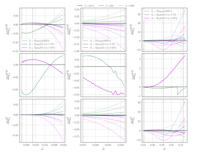
Figure 11: This Figure is the equivalent of Fig. 2 with TaylorF2 at 5.5PN PM and 7 PN tides (blue), 5.5PN PM and 7.5PN tides (magenta) and IMRPhenomPv2NRTidalv2 (green). Note that the 5.5PN PM and NRTidalv2 descriptions improve the $\Delta Q_{\hat{\omega}}^{PM}$ and $\Delta Q_{\hat{\omega}}^{T}$ in the low and high frequency regimes, respectively. When coupled to a 5.5PN PM, 7.5 PN tides are closer to TEOBResumS for $\tilde{\Lambda}=100$ than the 7PN description, which in turn performs better for $\tilde{\Lambda}=400$ over a large portion of the frequency range.

Figure 11 shows $Q_{\hat{\omega}}$ for the aforementioned approximants, computed for three reference signals with varying $\tilde{\Lambda}$ and zero spins, once again divided into three $\hat{\omega}$ intervals, correspoding to the regimes in which tidal contributions are roughly smaller than, comparable to or dominant with respect to $\Delta Q_{\hat{\omega}}^{PM}$. Inspecting the first column (which corresponds to the early frequencies interval), we notice that the $\Delta Q_{\hat{\omega}}^{PM}$ of TaylorF2 is comparable to that of IMRPhenomPv2NRTidalv2, and overall closer to TEOBResumS’ description than the one provided by considering a 3.5PN point mass baseline. When considering the tidal sector, instead, we note that the behaviours of NRTidalv2 and 7.5PN tides are opposites from the start. Moving to higher frequencies, tidal effects dominate both the late inspiral and merger regimes for both approximants. IMRPhenomPv2NRTidalv2 is less attractive than ${\tt IMRPhenomPv2NRTidal}$, while the 7.5 PN tidal description is more repulsive than the 6PN one. Close to merger we find that – as expected – the point mass contribution of the 5.5PN approximant becomes large and positive, and partially compensates the negative $\Delta Q_{\hat{\omega}}^{T}$. Overall, we find that IMRPhenomPv2NRTidalv2 provides a description that is much closer to TEOBResumS’ than the one offered by ${\tt IMRPhenomPv2NRTidal}$, albeit being still slightly more attractive.

Spinning configurations are studied in Fig. 12, which shows $\Delta Q_{\hat{\omega}}$ for three target signals with $\tilde{\Lambda}=400$ and increasing spins $\chi_{1}=\chi_{2}$. Focusing on the low frequency contribution to $\Delta Q_{\hat{\omega}}$, we observe that IMRPhenomPv2NRTidalv2 is now overall closer to TEOBResumS than IMRPhenomPv2NRtidal and TaylorF2 were. Additionally, the 5.5 PN point mass, which in the non-spinning case follows closely the behaviour of TEOBResumS, becomes increasingly more negative as spins grow. Moving to the high frequency regime, the improvements of NRTidalv2 have a positive effect on $\Delta Q_{\hat{\omega}}^{T}$ of the phenomenological approximant. Indeed, while the Phenom-EOB-PN hierarchy displayed in Fig. 3 for spinning binaries is mantained, the differences decrease and NRTidalv2 is closer to TEOBResumS’ description than NRTidal.

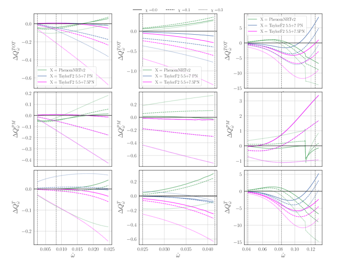
Figure 12: This Figure is the equivalent of Fig. 2 with TaylorF2 at 5.5PN PM and 7 PN tides (blue), 5.5PN PM and 7.5PN tides (magenta) and IMRPhenomPv2NRTidalv2 (green). We note that in the low frequency regime the 5.5PN PM, which gives the best approximation of the ${\tt TEOBResumS}$ PM between the approximants considered for nonspinning equal-mass binaries, becomes increasingly more negative as spins grow. On the other hand, the Phenom description over the same range consistently has $|\Delta Q_{\hat{\omega}}^{PM}|<0.2$. When considering the high frequency contributions, instead, the hierarchy displayed in Fig. 3 is mantained.

References

- Abbott et al. (2017a) B. P. Abbott et al. (Virgo, LIGO Scientific), Phys. Rev. Lett. 119, 161101 (2017a), arXiv:1710.05832 [gr-qc] .
- Radice et al. (2018) D. Radice, A. Perego, F. Zappa, and S. Bernuzzi, Astrophys. J. 852, L29 (2018), arXiv:1711.03647 [astro-ph.HE] .
- Abbott et al. (2018a) B. P. Abbott et al. (LIGO Scientific, Virgo), Phys. Rev. Lett. 121, 161101 (2018a), arXiv:1805.11581 [gr-qc] .
- Essick et al. (2020) R. Essick, P. Landry, and D. E. Holz, Phys. Rev. D 101, 063007 (2020), arXiv:1910.09740 [astro-ph.HE] .
- Abbott et al. (2020a) B. P. Abbott et al. (LIGO Scientific, Virgo), Class. Quant. Grav. 37, 045006 (2020a), arXiv:1908.01012 [gr-qc] .
- Ghosh et al. (2016) A. Ghosh, W. Del Pozzo, and P. Ajith, Phys. Rev. D 94, 104070 (2016), arXiv:1505.05607 [gr-qc] .
- Veitch et al. (2015) J. Veitch et al., Phys. Rev. D91, 042003 (2015), arXiv:1409.7215 [gr-qc] .
- Flanagan and Hinderer (2008) E. E. Flanagan and T. Hinderer, Phys.Rev. D77, 021502 (2008), arXiv:0709.1915 [astro-ph] .
- Damour and Nagar (2010) T. Damour and A. Nagar, Phys. Rev. D81, 084016 (2010), arXiv:0911.5041 [gr-qc] .
- Damour and Nagar (2011) T. Damour and A. Nagar, Mass and motion in general relativity. Proceedings, School on Mass, Orleans, France, June 23-25, 2008, Fundam. Theor. Phys. 162, 211 (2011), arXiv:0906.1769 [gr-qc] .
- Damour et al. (2015) T. Damour, P. Jaranowski, and G. Schäfer, Phys. Rev. D91, 084024 (2015), arXiv:1502.07245 [gr-qc] .
- Abbott et al. (2020b) B. Abbott et al. (LIGO Scientific, Virgo), Astrophys. J. Lett. 892, L3 (2020b), arXiv:2001.01761 [astro-ph.HE] .
- Abbott et al. (2019a) B. P. Abbott et al. (LIGO Scientific, Virgo), Phys. Rev. X9, 031040 (2019a), arXiv:1811.12907 [astro-ph.HE] .
- Dudi et al. (2018) R. Dudi, F. Pannarale, T. Dietrich, M. Hannam, S. Bernuzzi, F. Ohme, and B. Bruegmann, (2018), arXiv:1808.09749 [gr-qc] .
- Samajdar and Dietrich (2018) A. Samajdar and T. Dietrich, Phys. Rev. D98, 124030 (2018), arXiv:1810.03936 [gr-qc] .
- Samajdar and Dietrich (2019) A. Samajdar and T. Dietrich, Phys. Rev. D100, 024046 (2019), arXiv:1905.03118 [gr-qc] .
- Messina et al. (2019) F. Messina, R. Dudi, A. Nagar, and S. Bernuzzi, Phys. Rev. D99, 124051 (2019), arXiv:1904.09558 [gr-qc] .
- Agathos et al. (2020) M. Agathos, F. Zappa, S. Bernuzzi, A. Perego, M. Breschi, and D. Radice, Phys. Rev. D101, 044006 (2020), arXiv:1908.05442 [gr-qc] .
- Narikawa et al. (2019) T. Narikawa, N. Uchikata, K. Kawaguchi, K. Kiuchi, K. Kyutoku, M. Shibata, and H. Tagoshi, (2019), arXiv:1910.08971 [gr-qc] .
- Chen et al. (2020) A. Chen, N. K. Johnson-McDaniel, T. Dietrich, and R. Dudi, Phys. Rev. D 101, 103008 (2020), arXiv:2001.11470 [astro-ph.HE] .
- Sathyaprakash et al. (2011) B. Sathyaprakash et al., in 46th Rencontres de Moriond on Gravitational Waves and Experimental Gravity (2011) pp. 127–136, arXiv:1108.1423 [gr-qc] .
- Aasi et al. (2015) J. Aasi et al. (LIGO Scientific), Class. Quant. Grav. 32, 074001 (2015), arXiv:1411.4547 [gr-qc] .
- Abbott et al. (2018b) B. P. Abbott et al. (VIRGO, KAGRA, LIGO Scientific), Living Rev. Rel. 21, 3 (2018b), [Living Rev. Rel.19,1(2016)], arXiv:1304.0670 [gr-qc] .
- Harry (2010) G. M. Harry (LIGO Scientific Collaboration), Class.Quant.Grav. 27, 084006 (2010).
- Acernese et al. (2015) F. Acernese et al. (VIRGO), Class. Quant. Grav. 32, 024001 (2015), arXiv:1408.3978 [gr-qc] .
- Maggiore et al. (2020) M. Maggiore et al., JCAP 03, 050 (2020), arXiv:1912.02622 [astro-ph.CO] .
- Cutler and Vallisneri (2007) C. Cutler and M. Vallisneri, Phys. Rev. D 76, 104018 (2007), arXiv:0707.2982 [gr-qc] .
- Favata (2014) M. Favata, Phys.Rev.Lett. 112, 101101 (2014), arXiv:1310.8288 [gr-qc] .
- Hinderer (2008) T. Hinderer, Astrophys.J. 677, 1216 (2008), arXiv:0711.2420 [astro-ph] .
- Damour and Nagar (2009) T. Damour and A. Nagar, Phys. Rev. D80, 084035 (2009), arXiv:0906.0096 [gr-qc] .
- Yagi (2014) K. Yagi, Phys. Rev. D89, 043011 (2014), arXiv:1311.0872 [gr-qc] .
- Owen and Sathyaprakash (1999) B. J. Owen and B. Sathyaprakash, Phys. Rev. D 60, 022002 (1999), arXiv:gr-qc/9808076 .
- Damour et al. (1998) T. Damour, B. R. Iyer, and B. S. Sathyaprakash, Phys. Rev. D57, 885 (1998), arXiv:gr-qc/9708034 [gr-qc] .
- Damour et al. (2011) T. Damour, A. Nagar, and M. Trias, Phys. Rev. D83, 024006 (2011), arXiv:1009.5998 [gr-qc] .
- Lindblom et al. (2008) L. Lindblom, B. J. Owen, and D. A. Brown, Phys.Rev. D78, 124020 (2008), arXiv:0809.3844 [gr-qc] .
- Cutler and Flanagan (1994) C. Cutler and E. E. Flanagan, Phys.Rev. D49, 2658 (1994), arXiv:gr-qc/9402014 [gr-qc] .
- Poisson and Will (1995) E. Poisson and C. M. Will, Phys.Rev. D52, 848 (1995), arXiv:gr-qc/9502040 [gr-qc] .
- Damour et al. (2012) T. Damour, A. Nagar, and L. Villain, Phys.Rev. D85, 123007 (2012), arXiv:1203.4352 [gr-qc] .
- Harry and Hinderer (2018) I. Harry and T. Hinderer, Class. Quant. Grav. 35, 145010 (2018), arXiv:1801.09972 [gr-qc] .
- Aso et al. (2013) Y. Aso, Y. Michimura, K. Somiya, M. Ando, O. Miyakawa, T. Sekiguchi, D. Tatsumi, and H. Yamamoto (KAGRA), Phys. Rev. D 88, 043007 (2013), arXiv:1306.6747 [gr-qc] .
- Akutsu et al. (2019) T. Akutsu et al. (KAGRA), Nature Astron. 3, 35 (2019), arXiv:1811.08079 [gr-qc] .
- Punturo et al. (2010) M. Punturo, M. Abernathy, F. Acernese, B. Allen, N. Andersson, et al., Class.Quant.Grav. 27, 194002 (2010).
- Hild et al. (2011) S. Hild et al., Class. Quant. Grav. 28, 094013 (2011), arXiv:1012.0908 [gr-qc] .
- Chatziioannou et al. (2017) K. Chatziioannou, A. Klein, N. Yunes, and N. Cornish, Phys. Rev. D95, 104004 (2017), arXiv:1703.03967 [gr-qc] .
- Kastaun and Ohme (2019) W. Kastaun and F. Ohme, Phys. Rev. D 100, 103023 (2019), arXiv:1909.12718 [gr-qc] .
- Vallisneri (2008) M. Vallisneri, Phys.Rev. D77, 042001 (2008), arXiv:gr-qc/0703086 [GR-QC] .
- Blanchet (2014) L. Blanchet, Living Rev. Relativity 17, 2 (2014), arXiv:1310.1528 [gr-qc] .
- Buonanno et al. (2009) A. Buonanno, B. Iyer, E. Ochsner, Y. Pan, and B. Sathyaprakash, Phys.Rev. D80, 084043 (2009), arXiv:0907.0700 [gr-qc] .
- Buonanno and Damour (1999) A. Buonanno and T. Damour, Phys. Rev. D59, 084006 (1999), arXiv:gr-qc/9811091 .
- Buonanno and Damour (2000) A. Buonanno and T. Damour, Phys. Rev. D62, 064015 (2000), arXiv:gr-qc/0001013 .
- Damour et al. (2000) T. Damour, P. Jaranowski, and G. Schaefer, Phys. Rev. D62, 084011 (2000), arXiv:gr-qc/0005034 [gr-qc] .
- Damour (2001) T. Damour, Phys. Rev. D64, 124013 (2001), arXiv:gr-qc/0103018 .
- Damour et al. (2008) T. Damour, P. Jaranowski, and G. Schäfer, Phys.Rev. D78, 024009 (2008), arXiv:0803.0915 [gr-qc] .
- Bini et al. (2019) D. Bini, T. Damour, and A. Geralico, Phys. Rev. Lett. 123, 231104 (2019), arXiv:1909.02375 [gr-qc] .
- Bini et al. (2020a) D. Bini, T. Damour, and A. Geralico, Phys. Rev. D 102, 024062 (2020a), arXiv:2003.11891 [gr-qc] .
- Bini et al. (2020b) D. Bini, T. Damour, and A. Geralico, Phys. Rev. D 102, 024061 (2020b), arXiv:2004.05407 [gr-qc] .
- Santamaria et al. (2010) L. Santamaria, F. Ohme, P. Ajith, B. Brügmann, N. Dorband, et al., Phys.Rev. D82, 064016 (2010), arXiv:1005.3306 [gr-qc] .
- Hannam et al. (2014) M. Hannam, P. Schmidt, A. Bohé, L. Haegel, S. Husa, F. Ohme, G. Pratten, and M. Pürrer, Phys. Rev. Lett. 113, 151101 (2014), arXiv:1308.3271 [gr-qc] .
- Khan et al. (2016) S. Khan, S. Husa, M. Hannam, F. Ohme, M. Pürrer, X. Jiménez Forteza, and A. Bohé, Phys. Rev. D93, 044007 (2016), arXiv:1508.07253 [gr-qc] .
- Husa et al. (2016) S. Husa, S. Khan, M. Hannam, M. Pürrer, F. Ohme, X. Jiménez Forteza, and A. Bohé, Phys. Rev. D93, 044006 (2016), arXiv:1508.07250 [gr-qc] .
- London et al. (2018) L. London, S. Khan, E. Fauchon-Jones, X. J. Forteza, M. Hannam, S. Husa, C. Kalaghatgi, F. Ohme, and F. Pannarale, Phys. Rev. Lett. 120, 161102 (2018), arXiv:1708.00404 [gr-qc] .
- García-Quirós et al. (2020) C. García-Quirós, M. Colleoni, S. Husa, H. Estellés, G. Pratten, A. Ramos-Buades, M. Mateu-Lucena, and R. Jaume, (2020), arXiv:2001.10914 [gr-qc] .
- Pratten et al. (2020a) G. Pratten, S. Husa, C. Garcia-Quiros, M. Colleoni, A. Ramos-Buades, H. Estelles, and R. Jaume, (2020a), arXiv:2001.11412 [gr-qc] .
- Pratten et al. (2020b) G. Pratten et al., (2020b), arXiv:2004.06503 [gr-qc] .
- Arun et al. (2009) K. G. Arun, A. Buonanno, G. Faye, and E. Ochsner, Phys. Rev. D79, 104023 (2009), [Erratum: Phys. Rev.D84,049901(2011)], arXiv:0810.5336 [gr-qc] .
- Mikoczi et al. (2005) B. Mikoczi, M. Vasuth, and L. A. Gergely, Phys. Rev. D 71, 124043 (2005), arXiv:astro-ph/0504538 .
- Vines et al. (2011) J. Vines, E. E. Flanagan, and T. Hinderer, Phys. Rev. D83, 084051 (2011), arXiv:1101.1673 [gr-qc] .
- Henry et al. (2020) Q. Henry, G. Faye, and L. Blanchet, (2020), arXiv:2005.13367 [gr-qc] .
- Nagar et al. (2018) A. Nagar et al., Phys. Rev. D98, 104052 (2018), arXiv:1806.01772 [gr-qc] .
- Damour and Nagar (2014) T. Damour and A. Nagar, Phys.Rev. D90, 044018 (2014), arXiv:1406.6913 [gr-qc] .
- Nagar et al. (2017) A. Nagar, G. Riemenschneider, and G. Pratten, Phys. Rev. D96, 084045 (2017), arXiv:1703.06814 [gr-qc] .
- Nagar et al. (2019a) A. Nagar, F. Messina, P. Rettegno, D. Bini, T. Damour, A. Geralico, S. Akcay, and S. Bernuzzi, Phys. Rev. D99, 044007 (2019a), arXiv:1812.07923 [gr-qc] .
- Nagar et al. (2019b) A. Nagar, G. Pratten, G. Riemenschneider, and R. Gamba, (2019b), arXiv:1904.09550 [gr-qc] .
- Nagar et al. (2020) A. Nagar, G. Riemenschneider, G. Pratten, P. Rettegno, and F. Messina, (2020), arXiv:2001.09082 [gr-qc] .
- Akcay et al. (2019) S. Akcay, S. Bernuzzi, F. Messina, A. Nagar, N. Ortiz, and P. Rettegno, Phys. Rev. D99, 044051 (2019), arXiv:1812.02744 [gr-qc] .
- Bernuzzi et al. (2015a) S. Bernuzzi, T. Dietrich, and A. Nagar, Phys. Rev. Lett. 115, 091101 (2015a), arXiv:1504.01764 [gr-qc] .
- Bini et al. (2012) D. Bini, T. Damour, and G. Faye, Phys.Rev. D85, 124034 (2012), arXiv:1202.3565 [gr-qc] .
- Bini and Damour (2014) D. Bini and T. Damour, Phys.Rev. D90, 124037 (2014), arXiv:1409.6933 [gr-qc] .
- Damour et al. (2013) T. Damour, A. Nagar, and S. Bernuzzi, Phys.Rev. D87, 084035 (2013), arXiv:1212.4357 [gr-qc] .
- Nagar and Rettegno (2019) A. Nagar and P. Rettegno, Phys. Rev. D99, 021501 (2019), arXiv:1805.03891 [gr-qc] .
- Pan et al. (2014) Y. Pan, A. Buonanno, A. Taracchini, M. Boyle, L. E. Kidder, et al., Phys.Rev. D89, 061501 (2014), arXiv:1311.2565 [gr-qc] .
- Babak et al. (2017) S. Babak, A. Taracchini, and A. Buonanno, Phys. Rev. D95, 024010 (2017), arXiv:1607.05661 [gr-qc] .
- Rettegno et al. (2019) P. Rettegno, F. Martinetti, A. Nagar, D. Bini, G. Riemenschneider, and T. Damour, (2019), arXiv:1911.10818 [gr-qc] .
- Hinderer et al. (2016) T. Hinderer et al., Phys. Rev. Lett. 116, 181101 (2016), arXiv:1602.00599 [gr-qc] .
- Steinhoff et al. (2016) J. Steinhoff, T. Hinderer, A. Buonanno, and A. Taracchini, Phys. Rev. D94, 104028 (2016), arXiv:1608.01907 [gr-qc] .
- Bohé et al. (2017) A. Bohé et al., Phys. Rev. D95, 044028 (2017), arXiv:1611.03703 [gr-qc] .
- Lackey et al. (2018) B. D. Lackey, M. Pürrer, A. Taracchini, and S. Marsat, (2018), arXiv:1812.08643 [gr-qc] .
- Messina and Nagar (2017) F. Messina and A. Nagar, Phys. Rev. D95, 124001 (2017), [Erratum: Phys. Rev.D96,no.4,049907(2017)], arXiv:1703.08107 [gr-qc] .
- Dietrich et al. (2017a) T. Dietrich, S. Bernuzzi, and W. Tichy, Phys. Rev. D96, 121501 (2017a), arXiv:1706.02969 [gr-qc] .
- Dietrich et al. (2019) T. Dietrich, A. Samajdar, S. Khan, N. K. Johnson-McDaniel, R. Dudi, and W. Tichy, Phys. Rev. D100, 044003 (2019), arXiv:1905.06011 [gr-qc] .
- Baiotti et al. (2011) L. Baiotti, T. Damour, B. Giacomazzo, A. Nagar, and L. Rezzolla, Phys. Rev. D84, 024017 (2011), arXiv:1103.3874 [gr-qc] .
- Baiotti et al. (2010) L. Baiotti, T. Damour, B. Giacomazzo, A. Nagar, and L. Rezzolla, Phys. Rev. Lett. 105, 261101 (2010), arXiv:1009.0521 [gr-qc] .
- Poisson (1998) E. Poisson, Phys. Rev. D57, 5287 (1998), arXiv:gr-qc/9709032 [gr-qc] .
- Bernuzzi et al. (2012a) S. Bernuzzi, A. Nagar, M. Thierfelder, and B. Brügmann, Phys.Rev. D86, 044030 (2012a), arXiv:1205.3403 [gr-qc] .
- Dietrich et al. (2017b) T. Dietrich, S. Bernuzzi, M. Ujevic, and W. Tichy, Phys. Rev. D95, 044045 (2017b), arXiv:1611.07367 [gr-qc] .
- Abbott et al. (2017b) B. P. Abbott et al. (GROND, SALT Group, OzGrav, DFN, INTEGRAL, Virgo, Insight-Hxmt, MAXI Team, Fermi-LAT, J-GEM, RATIR, IceCube, CAASTRO, LWA, ePESSTO, GRAWITA, RIMAS, SKA South Africa/MeerKAT, H.E.S.S., 1M2H Team, IKI-GW Follow-up, Fermi GBM, Pi of Sky, DWF (Deeper Wider Faster Program), Dark Energy Survey, MASTER, AstroSat Cadmium Zinc Telluride Imager Team, Swift, Pierre Auger, ASKAP, VINROUGE, JAGWAR, Chandra Team at McGill University, TTU-NRAO, GROWTH, AGILE Team, MWA, ATCA, AST3, TOROS, Pan-STARRS, NuSTAR, ATLAS Telescopes, BOOTES, CaltechNRAO, LIGO Scientific, High Time Resolution Universe Survey, Nordic Optical Telescope, Las Cumbres Observatory Group, TZAC Consortium, LOFAR, IPN, DLT40, Texas Tech University, HAWC, ANTARES, KU, Dark Energy Camera GW-EM, CALET, Euro VLBI Team, ALMA), Astrophys. J. 848, L12 (2017b), arXiv:1710.05833 [astro-ph.HE] .
- LIGO Scientific Collaboration (2018) LIGO Scientific Collaboration, “LIGO Algorithm Library - LALSuite,” free software (GPL) (2018).
- Veitch and Vecchio (2010) J. Veitch and A. Vecchio, Phys.Rev. D81, 062003 (2010), arXiv:0911.3820 [astro-ph.CO] .
- Lindblom (2010) L. Lindblom, Phys. Rev. D82, 103011 (2010), arXiv:1009.0738 [astro-ph.HE] .
- Carney et al. (2018) M. F. Carney, L. E. Wade, and B. S. Irwin, Phys. Rev. D98, 063004 (2018), arXiv:1805.11217 [gr-qc] .
- Racine (2008) E. Racine, Phys. Rev. D78, 044021 (2008), arXiv:0803.1820 [gr-qc] .
- Baird et al. (2013) E. Baird, S. Fairhurst, M. Hannam, and P. Murphy, Phys. Rev. D 87, 024035 (2013), arXiv:1211.0546 [gr-qc] .
- De et al. (2018) S. De, D. Finstad, J. M. Lattimer, D. A. Brown, E. Berger, and C. M. Biwer, Phys. Rev. Lett. 121, 091102 (2018), [Erratum: Phys. Rev. Lett.121,no.25,259902(2018)], arXiv:1804.08583 [astro-ph.HE] .
- Yagi and Yunes (2016) K. Yagi and N. Yunes, Class. Quant. Grav. 33, 13LT01 (2016), arXiv:1512.02639 [gr-qc] .
- Yagi and Yunes (2017) K. Yagi and N. Yunes, Phys. Rept. 681, 1 (2017), arXiv:1608.02582 [gr-qc] .
- Raithel (2019) C. A. Raithel, Eur. Phys. J. A 55, 80 (2019), arXiv:1904.10002 [astro-ph.HE] .
- Read et al. (2009) J. S. Read, B. D. Lackey, B. J. Owen, and J. L. Friedman, Phys. Rev. D79, 124032 (2009), arXiv:0812.2163 [astro-ph] .
- Raaijmakers et al. (2018) G. Raaijmakers, T. Riley, and A. Watts, Mon. Not. Roy. Astron. Soc. 478, 2177 (2018), arXiv:1804.09087 [astro-ph.HE] .
- Lindblom and Indik (2014) L. Lindblom and N. M. Indik, Phys. Rev. D 89, 064003 (2014), [Erratum: Phys.Rev.D 93, 129903 (2016)], arXiv:1310.0803 [astro-ph.HE] .
- Nitz et al. (2020) A. Nitz, I. Harry, D. Brown, C. M. Biwer, J. Willis, T. D. Canton, C. Capano, L. Pekowsky, T. Dent, A. R. Williamson, G. S. Davies, S. De, M. Cabero, B. Machenschalk, P. Kumar, S. Reyes, D. Macleod, F. Pannarale, dfinstad, T. Massinger, M. Tápai, L. Singer, S. Khan, S. Fairhurst, S. Kumar, A. Nielsen, SSingh087, shasvath, I. Dorrington, and B. U. V. Gadre, “gwastro/pycbc: Pycbc release v1.16.9,” (2020).
- Romero-Shaw et al. (2020) I. Romero-Shaw et al., (2020), arXiv:2006.00714 [astro-ph.IM] .
- Breschi et al. (2019) M. Breschi, S. Bernuzzi, F. Zappa, M. Agathos, A. Perego, D. Radice, and A. Nagar, Phys. Rev. D100, 104029 (2019), arXiv:1908.11418 [gr-qc] .
- Smith and Ashton (2019) R. Smith and G. Ashton, (2019), arXiv:1909.11873 [gr-qc] .
- Abbott et al. (2019b) R. Abbott et al. (LIGO Scientific, Virgo), (2019b), arXiv:1912.11716 [gr-qc] .
- Bernuzzi et al. (2015b) S. Bernuzzi, A. Nagar, T. Dietrich, and T. Damour, Phys.Rev.Lett. 114, 161103 (2015b), arXiv:1412.4553 [gr-qc] .
- Abbott et al. (2019c) B. P. Abbott et al. (LIGO Scientific, Virgo), Phys. Rev. X9, 011001 (2019c), arXiv:1805.11579 [gr-qc] .
- Dai et al. (2018) L. Dai, T. Venumadhav, and B. Zackay, (2018), arXiv:1806.08793 [gr-qc] .
- Zackay et al. (2018) B. Zackay, L. Dai, and T. Venumadhav, (2018), arXiv:1806.08792 [astro-ph.IM] .
- Radice and Dai (2019) D. Radice and L. Dai, Eur. Phys. J. A55, 50 (2019), arXiv:1810.12917 [astro-ph.HE] .
- Raaijmakers et al. (2019) G. Raaijmakers et al., Astrophys. J. Lett. 887, L22 (2019), arXiv:1912.05703 [astro-ph.HE] .
- Raaijmakers et al. (2020) G. Raaijmakers et al., Astrophys. J. Lett. 893, L21 (2020), arXiv:1912.11031 [astro-ph.HE] .
- Reitze et al. (2019) D. Reitze et al., Bull. Am. Astron. Soc. 51, 035 (2019), arXiv:1907.04833 [astro-ph.IM] .
- Abbott et al. (2017c) B. P. Abbott et al. (LIGO Scientific), Class. Quant. Grav. 34, 044001 (2017c), arXiv:1607.08697 [astro-ph.IM] .
- Annala et al. (2018) E. Annala, T. Gorda, A. Kurkela, and A. Vuorinen, Phys. Rev. Lett. 120, 172703 (2018), arXiv:1711.02644 [astro-ph.HE] .
- Capano et al. (2020) C. D. Capano, I. Tews, S. M. Brown, B. Margalit, S. De, S. Kumar, D. A. Brown, B. Krishnan, and S. Reddy, Nature Astron. 4, 625 (2020), arXiv:1908.10352 [astro-ph.HE] .
- Bernuzzi et al. (2012b) S. Bernuzzi, M. Thierfelder, and B. Brügmann, Phys.Rev. D85, 104030 (2012b), arXiv:1109.3611 [gr-qc] .
- Radice et al. (2014) D. Radice, L. Rezzolla, and F. Galeazzi, Mon.Not.Roy.Astron.Soc. 437, L46 (2014), arXiv:1306.6052 [gr-qc] .
- Radice et al. (2016) D. Radice, S. Bernuzzi, and C. D. Ott, Phys. Rev. D94, 064011 (2016), arXiv:1603.05726 [gr-qc] .
- Bernuzzi and Dietrich (2016) S. Bernuzzi and T. Dietrich, Phys. Rev. D94, 064062 (2016), arXiv:1604.07999 [gr-qc] .
- Dietrich et al. (2018a) T. Dietrich, D. Radice, S. Bernuzzi, F. Zappa, A. Perego, B. Brügmann, S. V. Chaurasia, R. Dudi, W. Tichy, and M. Ujevic, Class. Quant. Grav. 35, 24LT01 (2018a), arXiv:1806.01625 [gr-qc] .
- Bernuzzi et al. (2014) S. Bernuzzi, A. Nagar, S. Balmelli, T. Dietrich, and M. Ujevic, Phys.Rev.Lett. 112, 201101 (2014), arXiv:1402.6244 [gr-qc] .
- Dietrich et al. (2017c) T. Dietrich, M. Ujevic, W. Tichy, S. Bernuzzi, and B. Brügmann, Phys. Rev. D95, 024029 (2017c), arXiv:1607.06636 [gr-qc] .
- Dietrich and Hinderer (2017) T. Dietrich and T. Hinderer, Phys. Rev. D95, 124006 (2017), arXiv:1702.02053 [gr-qc] .
- Dietrich et al. (2018b) T. Dietrich, S. Bernuzzi, B. Brügmann, M. Ujevic, and W. Tichy, Phys. Rev. D97, 064002 (2018b), arXiv:1712.02992 [gr-qc] .
- Chatziioannou et al. (2018) K. Chatziioannou, C.-J. Haster, and A. Zimmerman, Phys. Rev. D97, 104036 (2018), arXiv:1804.03221 [gr-qc] .