Kilohertz Gravitational Waves from Binary Neutron Star Mergers:
Inference of Postmerger Signals with the Einstein Telescope

Abstract

Next-generation detectors are expected to be sensitive to postmerger signals from binary neutron star coalescences and thus to directly probe the remnant dynamics. We investigate the scientific potential of postmerger detections with the Einstein Telescope using full Bayesian analyses with the state of the art waveform model NRPMw. We find that: (i) Postmerger signals with SNR ${\sim}7$ can be confidently detected with a Bayes’ factor of $\log\mathcal{B}\simeq 5$ (${\rm e}$-folded) and the posterior distributions report informative measurements already at SNR ${\sim}6$ for some noise realizations. (ii) The postmerger peak frequency $f_{2}$ can be confidently identified at SNR $7$ with errors of $O(1~{}{\rm kHz})$, that decrease below $O(100~{}{\rm Hz})$ for SNR 10. (iii) The remnant’s time of collapse to black hole can be constrained to $O(20~{}{\rm ms})$ at SNR 10. However, the inference can be biased by noise fluctuations if the latter exceed the signal’s amplitude before collapse. (iv) Violations of the EOS-insentive relations for $f_{2}$ can be detected at SNR $\gtrsim 8$ if the frequency shifts are $\gtrsim 500~{}{\rm Hz}$; they can be smoking guns for EOS softening effects at extreme densities. However, the $f_{2}$ measurement can be significantly biased by subdominant frequency components for short-lived remnants. In these cases, an EOS softening might be better inferred from the remnant’s earlier collapse.

I Introduction

Third-generation gravitational-wave (GW) observatories, such as Einstein Telescope (ET) Hild et al. (2008), will observe gravitational radiation from binary neutron star (BNS) remnants. The detection of postmerger (PM) gravitational transients will give the most direct access to the merger outcome by probing the nature of the compact object in the remnant, see e.g. Radice et al. (2020); Bernuzzi (2020) for recent reviews. Moreover, if the remnant does not promptly collapse into black hole (BH), the PM radiation can provide information on the extreme density equation of state (EOS) of the neutron star (NS) remnant, thus impacting the nuclear physics of NSs Chatziioannou et al. (2017); Tsang et al. (2019); Breschi et al. (2019); Easter et al. (2020); Breschi et al. (2022a); Wijngaarden et al. (2022). In Ref. Breschi et al. (2022b) (Paper I hereafter) we have developed a novel PM model built on a wavelet basis and incorporating several NR-driven quasiuniversal relations. Here, we expand our investigations by exploring the capabilities of ET in Bayesian parameter estimation of PM signals. A follow-up paper of this series will report on full-spectrum analysis.

The Einstein Telescope Hild et al. (2008, 2011); Hild (2012); Punturo et al. (2010a, a, b); Maggiore et al. (2020); Sathyaprakash et al. (2011, 2012); Amann et al. (2020) is a triangularly-shaped underground infrastructure for GW observations, with a photodetector at each vertex measuring GW fluctuations with interferometric techniques and employing laser beams running along the adjacent sides at a 60 degree angle. Hence, the observatory is composed by three detectors. ET will improve the sensitivities of modern observatories by increasing the size of the interferometer from the $3~{}{\rm km}$ arm length of the Virgo detector to $10~{}{\rm km}$, and by implementing a series of new technologies. These include a cryogenic system, quantum technologies to reduce the laser fluctuations and noise-mitigation measures to reduce environmental perturbations. Moreover, the instrument will exploit a xylophone-design in which each GW detector is composed of two individual interferometers: a cryogenic low-power interferometer with sensitivity plateau in the low-frequency band, roughly between $7~{}{\rm Hz}$ and $20~{}{\rm Hz}$, and an high-power interferometer that covers the higher portion of the spectrum, roughly above ${\sim}100~{}{\rm Hz}$. The ET-D configuration discussed in Hild et al. (2011) and employed in this work has a sensitivity bucket covering the GW spectrum from ${\sim}5~{}{\rm Hz}$ up to ${\sim}3~{}{\rm kHz}$. Such broad-band sensitivity is ideal for BNS observations. Low-frequency measurements follow the binary evolution for many cycles before merger extracting precise measurements of the progenitor’s properties. In contrast, the high-frequency end, i.e. $\gtrsim 1~{}{\rm kHz}$, enables the detection of PM signals at sensitivities that are unreachable by current infrastructures.

The significant complexity of the PM source emission implies that standard PE techniques, relying on extremely accurate models parametrised by the minimal set of the system’s degrees of freedom, can no longer be applied. For this reason, recent Bayesian studies of BNS PM transients employed largely different modeling choices, ranging from signal-agnostic reconstructions to semi-agnostic descriptions calibrated on numerical simulations.data The advantage of agnostic techniques lies in an unbiased reconstruction of the signal, coming however at the price of losing information content buried in the noise. Semi-agnostic reconstructions, which can directly incorporate information from NR simulations, allow to dig deeper into the detector background and hence detect signals at lower signal-to-noise ratio (SNR). However such measurements require extensive training datasets and the inclusion of all the relevant contributions in order to provide a faithful recovery of the signal’s properties. An additional complication that arises when comparing different semi-agnostic approaches thus stems in the NR dataset used to built and validate them.

Chatziioannou et al. (2017) performed PE studies of BNS PM transients with model-independent Bayesian techniques, showing informative posteriors for PM SNR of ${\sim}5$ with a validation set of three NR simulations. However, the method employed in Ref. Chatziioannou et al. (2017) did not provide estimation of the evidence, making difficult a more direct and complete comparison with different techniques. Tsang et al. (2019) used a simplified model based on damped sinusoidal template that aims to characterize the dominant PM peak. This method recovered informative measurements for a threshold of SNR between $4$ and $8$ using a validation set of four binaries. Breschi et al. (2019) constructed the PM model employing NR-calibrated relations that naturally permits the attachment to pre-merger templates, introducing the first inspiral-merger-postmerger BNS model. This approach show detectabillity threshold for PM SNR ${\sim}8$ over a NR set of 10 binaries. The performances are improved in Ref. Breschi et al. (2022a) to SNR $7$, corresponding to a Bayes’ factor (BF) of ${\rm e}^{5}$, including model recalibration parameters in the PE routine (see also Paper I). Similarly to Tsang et al. (2019), Easter et al. (2020) modeled the PM spectrum employing a superposition of multiple damped sinusoidal components recovering PM transients for SNR $7$ over a validation set of nine binaries, which corresponds to a BF of ${\rm e}^{8}$. Wijngaarden et al. (2022) extended the approach of Ref. Chatziioannou et al. (2017) by including the pre-merger portion of data.

In this paper, we employ the novel NRPMw model Breschi et al. (2022b) for Bayesian studies of GW signals from BNS PM remnants with the next-generation detector ET, investigating the PE performances under different noise realizations. The paper is structured as follows. In Sec. II, we introduce the framework employed for producing our set of simulated signals, and our PE configurations. We perform a consistent simulation-recovery study with NRPMw in Sec. III. We discuss PE studies on NR data in Sec. IV, inspecting the detectability performances and the recovered posteriors on the signal parameters. In Sec. V, we reanalyze the softening case presented in Radice et al. (2017); Breschi et al. (2019) investigating extreme-matter tests for non-hadronic EOS. We conclude in Sec. VI.

Conventions –

All quantities are expressed in SI units, with masses in Solar masses ${\rm M_{\odot}}$ and distances in Mpc. Henceforth, the symbol ‘$\log$’ denotes the natural logarithm. The total binary mass is indicated with $M=m_{1}+m_{2}$, the mass ratio $q=m_{1}/m_{2}\geq 1$, and the symmetric mass ratio $\nu=m_{1}m_{2}/M^{2}$. The dimensionless spin vectors are denoted with ${\boldsymbol{\chi}}_{i}$ for $i=1,2$ and the spin component aligned with the orbital angular momentum L are labeled as $\chi_{i}={\boldsymbol{\chi}}_{i}\cdot\textbf{L}/|\textbf{L}|$. The effective spin parameter ${\chi_{\rm eff}}$ is a mass-weighted, aligned spin combination, i.e.

$${\chi_{\rm eff}}=\frac{m_{1}\chi_{1}+m_{2}\chi_{2}}{M}\,.$$ (1)

Moreover, the quadrupolar tidal deformability parameters are defined as $\Lambda_{i}=({2}/{3})\,k_{2,i}\,C_{i}^{-5}$ for $i=1,2$, where $k_{2,i}$ and $C_{i}$ are the second Love number and the compactness of the $i$-th object, respectively. The quadrupolar tidal polarizability $\kappa^{\rm T}_{2}$ is

$$\kappa^{\rm T}_{2}=3\nu\,\left[\left(\frac{m_{1}}{M}\right)^{3}\Lambda_{1}+(1\leftrightarrow 2)\right]\,.$$ (2)

Masses, spins, and tides define the intrinsic parameters of a BNS system, i.e. $\boldsymbol{\theta}_{\rm bin}=\{M,q,\chi_{1},\chi_{2},\Lambda_{1},\Lambda_{2}\}$. The extrinsic parameters of the source ${\boldsymbol{\theta}_{\rm ext}}=\{D_{L},\iota,\alpha,\delta,\psi,t_{\rm mrg},\phi_{\rm mrg}\}$, i.e. luminosity distance $D_{L}$, inclination angle $\iota$, right ascension angle $\alpha$, declination angle $\delta$, polarization angle $\psi$, time of coalescence $t_{\rm mrg}$, and phase at the merger $\phi_{\rm mrg}$, allow us to identify the location and orientation of the source. The PM model NRPMw is parameterized by two additional sets of degrees of freedom (see Paper I for a detailed discussion). The PM parameters ${\boldsymbol{\theta}_{\rm free}}=\{\phi_{\rm PM},t_{\rm coll},\alpha_{\rm peak}\}$ correspond to: the PM phase-shift $\phi_{\rm PM}$ that identifies the phase discontinuity after merger; the time of collapse $t_{\rm coll}$ that characterizes the collapse of the remnant into BH; and the frequency drift $\alpha_{\rm peak}$ that accounts for linear evolution of the dominant $f_{2}$ component. Moreover, we include the recalibration parameters ${\boldsymbol{\delta}_{\rm fit}}$ that account for deviations from the predictions of the EOS-insensitive relations consistently with the related theoretical uncertainties.

II Framework

In this section, we discuss the framework employed to generate and analyze the artificial data, called “injections”. We discuss the injections creation in Sec. II.1, the PE settings are reported in Sec. II.2 and we discuss the treatment of different noise realizations in Sec. II.3. All the analyses are performed with the publicly available bajes pipeline Breschi et al. (2021).

II.1 Injection settings

We generate artificial data for the triangular, triple-interferometer ET detector Hild et al. (2008); Punturo et al. (2010a); Maggiore et al. (2020), segmented into chunks of $1~{}{\rm s}$ duration with a sampling rate of $16384~{}{\rm Hz}$. For each detector $i$, the artificial data series $d_{i}(t)=s_{i}(t)+n_{i}(t)$ is composed of the signal $s_{i}(t)$ projected onto the $i$-th detector and the respective noise contribution $n_{i}(t)$. We label with bold symbols the sets ${\text{{s}}}(t)=\{s_{i}(t)\}$, ${\text{{n}}}(t)=\{n_{i}(t)\}$, and ${\text{{d}}}(t)=\{d_{i}(t)\}$ such that ${\text{{d}}}(t)={\text{{s}}}(t)+{\text{{n}}}(t)$. The injected signals vary depending on the study: in Sec. III, the signal is taken to be identical to NRPMw for a fixed set of parameters in order to perform a consistent injection-recovery test; while, in Sec. IV, we inject NR templates in order to study the performance of NRPMw in a more realistic scenario. The noise is assumed to be Gaussian, wide-sense stationary, and colored according to the power spectral density (PSD) expected for ET-D Hild (2012).

Given a data series $d$ and a template $h$, we introduce the matched-filtered SNR $\rho$ as

$$\rho(h)=\frac{(d|h)}{\sqrt{(h|h)}}\,,$$ (3)

where the inner product $(\cdot|\cdot)$ between two time-series, say $a(t)$ and $b(t)$, corresponds to

$$(a|b)=4\Re\int\frac{a^{*}(f)\,b(f)}{S_{n}(f)}\,{\rm d}f\,,$$ (4)

where $a(f)$ and $b(f)$ are the Fourier transforms respectively of $a(t)$ and $b(t)$, and $S_{n}(f)$ is the PSD employed to generate the noise segments. The definition Eq. (3) can be extended to multiple detectors employing quadrature summation. Then, we label $\rho_{\rm inj}=\rho(s)$ the ratio computed with the exact injected template; while, $\rho_{\rm rec}=\rho(h_{\text{{\tt NRPMw}}})$ is the SNR recovered with the NRPMw template $h_{\text{{\tt NRPMw}}}$. The templates $s(t)$ are injected at seven different SNRs $\rho_{\rm inj}=\{5,6,6.5,7,7.5,8,10\}$, which corresponds to locating the binaries at different luminosity distances. Moreover, the simulated binaries are oriented with $\iota=0$, $\psi=0$, and optimal sky position for the employed detector $\{\alpha=2.621,\delta=0.706\}$. Moreover, each artificial signal is analyzed employing five random noise realizations (see Sec. II.3).

II.2 Parameter estimation

The PE studies on the artificial data are performed with the nested sampling algorithm ultranest Buchner (2021) with 3000 initial live points. For a fixed set of data ${\text{{d}}}(t)$ the likelihood function $p({\text{{d}}}|\boldsymbol{\theta},H_{\rm S})$ Veitch et al. (2015); Breschi et al. (2021) is given by

$$\log p({\text{{d}}}|\boldsymbol{\theta},H_{\rm S})\propto-\frac{1}{2}\sum_{i}\big{(}d-h(\boldsymbol{\theta})\big{|}d-h(\boldsymbol{\theta})\big{)}_{i}\,,$$ (5)

where $H_{\rm S}$ represents the signal hypothesis. The subscript $i$ runs over the employed detectors and it denotes that the inner products are estimated with the corresponding data series, projected waveform, and PSD for each detector. The inner product in Eq. (5) is integrated over the frequency range $[1,8]~{}{\rm kHz}$, in order to isolate the contribution from the PM signal. We perform analytical marginalization over reference time $t_{\rm mrg}$ and phase $\phi_{\rm mrg}$. Then, the information on the parameters $\boldsymbol{\theta}$ is encoded in the posterior distribution $p(\boldsymbol{\theta}|{\text{{d}}},H_{\rm S})$, that can be estimated with Bayes’ theorem as

$$p(\boldsymbol{\theta}|{\text{{d}}},H_{\rm S})\propto p({\text{{d}}}|\boldsymbol{\theta},H_{\rm S})\,p(\boldsymbol{\theta}|H_{\rm S})\,.$$ (6)

Resorting to a nested sampling algorithm Skilling (2006), allows to straightforwardly and accurately estimate the evidence integral:

$$p({\text{{d}}}|H_{\rm S})=\int p({\text{{d}}}|\boldsymbol{\theta},H_{\rm S})\,p(\boldsymbol{\theta}|H_{\rm S})\,{\rm d}\boldsymbol{\theta}\,,$$ (7)

that in turns allows to compute the BF ($\mathcal{B}$) of the signal hypothesis against the noise hypothesis as $\mathcal{B}=p({\text{{d}}}|H_{\rm S})/p({\text{{d}}}|H_{\rm N})$. The noise hypothesis $H_{\rm N}$ corresponds to the assumption that no signal is included in the recorded data. We fix the nominal detectability threshold at $\log\mathcal{B}=5$ Kass and Raftery (1995).

The sampling is performed in total mass $M\in[1,6]~{}{\rm M_{\odot}}$ and mass ratio $q\in[1,2]$, differently to what is presented in Breschi et al. (2019, 2021), due to the analytical form of the empirical relations. In order to maintain a uniform prior in the mass components $m_{1,2}$, the prior $p(M,q|H_{\rm S})$ is modified according to Callister (2021). We include aligned spin parameters and employ an isotropic prior with the constraint $|\chi_{i}|\leq 0.2$ for $i=1,2$. Tidal parameters $\Lambda_{1}$ and $\Lambda_{2}$ are sampled with a uniform prior in the range $[0,4000]$. For the luminosity distance $D_{L}$, we use a volumetric prior in the range $[20,500]~{}{\rm Mpc}$ in order to confidently include the injected values. The remaining extrinsic parameters are treated according to Breschi et al. (2021). Moreover, we include the PM parameters ${\boldsymbol{\theta}_{\rm free}}$ in the PE routine and perform the sampling in the mass-scaled quantities using a uniform prior distribution for $t_{\rm coll}/M\in[t_{0}/M,3000]$, $M^{2}\alpha_{\rm peak}\in[-10^{-5},10^{-5}]$ and $\phi_{\rm PM}\in[0,2\pi]$. Finally, we introduce in the sampling the recalibration parameters ${\boldsymbol{\delta}_{\rm fit}}$ in order to account the intrinsic errors of the calibrated formulae. For these terms, we employ a normally distributed prior with zero mean and variance defined by the estimated relative errors (see Paper I).

II.3 Noise realizations

The near-threshold SNR of the signals under consideration requires additional care when extracting information from a simulation study. As such, in order to investigate the impact of noise fluctuations, we generate artificial data ${\text{{d}}}_{k}(t)={\text{{s}}}(t)+{\text{{n}}}_{k}(t)$ by injecting the targeted template ${\text{{s}}}(t)$ into different random noise realizations ${\text{{n}}}_{k}=\{n_{i}(t)\}_{k}$, where $i$ runs over the employed detectors and $k$ runs over the noise realizations. We employ a total of five different noise realizations fixing the initialization seed of the pseudo-random number generator in the bajes pipeline . The PE studies are performed on all the included realizations $k$ for each signal $s(t)$ and every injected SNR.

Once the posterior distributions $p(\boldsymbol{\theta}|{\text{{d}}}_{k},H_{\rm S})$ are estimated for each $k$, we compute an overall posterior in order to average over the different noise realizations. The overall posterior distribution is computed equally weighting each noise realization and averaging the recovered posteriors, i.e.

$$p(\boldsymbol{\theta}|{\text{{s}}},H_{\rm S})\propto\sum_{k}p(\boldsymbol{\theta}|{\text{{d}}}_{k},H_{\rm S})\,,$$ (8)

where $k$ runs over the employed noise realizations. This approach aims to estimate an agnostic and comprehensive posterior distribution that correctly incorporates the full statistical uncertainties. As we will show below, such uncertainties are relevant when discussing some of the cases under consideration. This estimate will improve with a larger number of noise configurations, $k\gg 1$, and is limited only by the computational cost.

III NRPMw injections

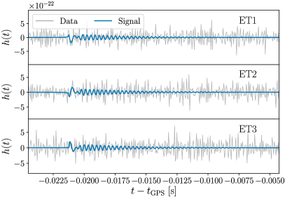
Figure 1: Injected PM signal (blue) and artificial data (gray) for an exemplary noise realization at PM SNR 8. The different panels show the time series for three ET interferometers. The signal corresponds to the NRPMw template computed for the parameters $M=2.82~{}{\rm M_{\odot}}$, $q=1.5$, $\kappa^{\rm T}_{2}=90$, $D_{L}=70~{}{\rm Mpc}$, $t_{\rm coll}=14~{}{\rm ms}$, $\alpha_{\rm peak}=0.021~{}{\rm kHz}^{2}$, $\phi_{\rm PM}=\pi/2$, and all recalibrations are identically zero, i.e. ${\boldsymbol{\delta}_{\rm fit}}=0$. The noise segments are generated assuming Gaussian and stationary noise according to ET-D PSD Hild (2012).

A first crucial step necessary to verify the reliability of a model and of the underlying Bayesian framework is a consistent injection-recovery study in which the simulated signal corresponds to a realization (for a given combination of $\boldsymbol{\theta}$) of the same model employed for recovery. In this way, it is possible to directly investigate sampling errors or possible complications due to poor modeling choices. Consequently, we employ NRPMw to generate the “real” signal $s(t)$ to be GW170817-like, setting total mass $M=2.82~{}{\rm M_{\odot}}$, mass ratio $q=1.5$, tidal polarizability $\kappa^{\rm T}_{2}=90$, time of collapse $t_{\rm coll}=14~{}{\rm ms}$, frequency drift $\alpha_{\rm peak}=0.021~{}{\rm kHz}^{2}$, PM phase $\phi_{\rm PM}=\pi/2$, and all recalibrations identically to zero, ${\boldsymbol{\delta}_{\rm fit}}=0$. Figure 1 shows the GW signals and the artificial data for each ET interferometer corresponding to an injection with PM SNR 8 for an exemplary noise realization.

We perform two sets of PE studies for this case. In the first set, we do not take into account the recalibrations ${\boldsymbol{\delta}_{\rm fit}}$; in the second set, we use recalibration in the PE analysis. The comparison between these two sets illustrates the effect of the recalibrations ${\boldsymbol{\delta}_{\rm fit}}$ on the recovered posterior distributions in the case where such recalibration is not required to correctly characterize the true signal, aiding the interpretation of the more complicated and realistic cases explored in the next sections. In general, it is expected that the inclusion of recalibrations will not introduce deviations in the mean values but will lead to a widening of the recovered posteriors due to the fluctuations associated with the calibrated relations, yielding more conservative measurements. In Sec. III.1, we discuss the recovered BFs and detectability threshold; while, the recovered posterior distributions are presented in Sec. III.2, comparing non-recalibrated and recalibrated PEs.

III.1 Detectability

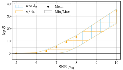
Figure 2: Logarithmic BFs, $\log\mathcal{B}$, as functions of the PM SNR $\rho_{\rm inj}$ of the injected NRPMw template. The analysis without recalibrations $\boldsymbol{\delta}_{\rm fit}$ is reported in blue; while, the recalibrated study is shown in orange. The dots refer to the mean values averaged over the different noise realizations and the shadowed areas correspond to the minimum and maximum values. Two horizontal lines identify $\log\mathcal{B}=0$ (black) and $\log\mathcal{B}=5$ (gray).

We investigate the BFs in favor of the signal hypothesis as function of the PM SNR of the injected transients, in order to understand the threshold required by NRPMw to perform an informative inference.

Figure 2 shows the recovered BFs for the injected binarys as function of the injected SNR, where the error-bars are estimated using the values recovered from different noise realization. In particular, we report the median values and the uncertainties are computed from the maximum and minimum estimates. The overall trend shows non-vanishing $\log\mathcal{B}$ for $\rho_{\rm inj}>6$ and the nominal threshold is reached at $\rho_{\rm inj}=7$. However, noise fluctuations can affect the recovered BFs, shifting the detectability threshold to SNRs of $\rho_{\rm inj}\simeq 8$. Above $\rho_{\rm inj}\simeq 8$, the errors of the recovered log-BFs appears to be roughly constant with values of ${\sim}15$ (considering the difference between the minimum and the maximum). Moreover, the recovered BFs are not affected by the introduction of the recalibration $\boldsymbol{\delta}_{\rm fit}$, since non-recalibrated NRPMw, i.e. without the inclusion of $\boldsymbol{\delta}_{\rm fit}$, is capable to fully reproduce the injected signal. The use of recalibrations is expected to be more important in the inference of signals that are not perfectly matched by the template model.

III.2 Posterior distributions

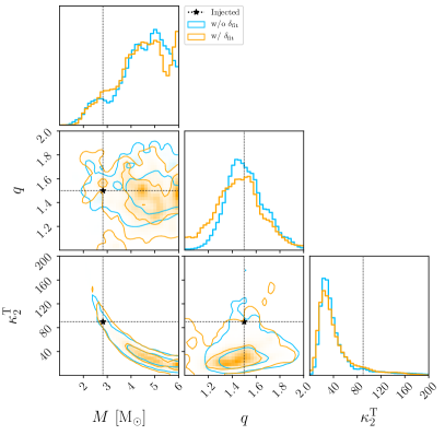
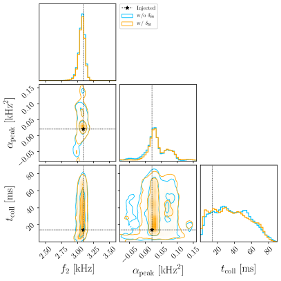
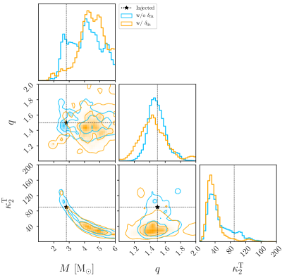
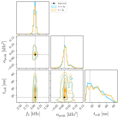
Figure 3: Posterior distributions for the binary parameters $\{M,q,\kappa^{\rm T}_{2}\}$ (left) and the PM parameters $\{f_{2},\alpha_{\rm peak},t_{\rm coll}\}$ (right) for the NRPMw injection-recovery study with SNR 8 (top) and SNR 10 (bottom). The reported posteriors correspond to the average distributions over all employed noise realizations. The blue lines show the non-recalibrated posteriors; while, the orange lines corresponds to the results that include the recalibrations $\boldsymbol{\delta}_{\rm fit}$. The contours show the 50% and 90% credibility regions. The injected values are reported with black dotted lines. The total mass $M$ and the tidal polarizability $\kappa^{\rm T}_{2}$ are generally biased due to the correlations introduced by the EOS-insensitive relations.

Figure 3 shows the posterior distributions recovered for SNR 8 and 10. The figures show the direct comparison between the non-recalibrated and the recalibrated posteriors. The results show negligible differences in the recovered parameters. The recalibrated inference shows, as expected, a small broadening of the posteriors. The recalibrated posteriors give a more conservative measurement because they take into account the uncertainties of the quasiuniversal relations.

At the considered SNRs, we find that the total mass is generally biased toward larger values, due to the correlations with other parameters, in particular with tidal polarizability $\kappa^{\rm T}_{2}$, luminosity distance $D_{L}$ and time of collapse $t_{\rm coll}$. Additional investigations with different prior boundaries for $M$ show that these biases persist also with larger upper bounds. As a consequence, the recovered tidal polarizabilities $\kappa^{\rm T}_{2}$ typically underestimate the true value due to the analytical form of the EOS-insensitive relations, as evident from the posterior contours in the $\{M,\kappa^{\rm T}_{2}\}$ plane. The posteriors slightly shrinks for increasing SNR, showing errors of ${\sim}1~{}{\rm M_{\odot}}$ and ${\sim}40$ respectively for $M$ and $\kappa^{\rm T}_{2}$ at SNR 10 and making the biases more evident. However, the injected values are included within the $90\%$ confidence levels up to SNR 10. These biases can be fixed introducing the pre-merger information in the PE routine (e.g. Breschi et al., 2019; Wijngaarden et al., 2022).

On the other hand, the mass ratio is well identified with errors of ${\sim}0.3$ at PM SNR 8, since it strongly correlates with the ratio of merger and PM amplitudes. Also the posteriors on the luminosity distance $D_{L}$ are generally consistent with the injected values with errors of $O(100~{}{\rm Mpc})$ at PM SNR 8. The frequency drift $\alpha_{\rm peak}$ and time of collapse $t_{\rm coll}$ show informative measurements that confidently include the injected values within the posterior support. However, these quantities are poorly constrained with errors comparable to the injected values. This is related to the nature of these terms: the parameters $\{\alpha_{\rm peak},t_{\rm coll}\}$ contribute to the late-time features of NRPMw affecting the length and the frequency evolution of the PM tail. This portion of the PM signal is typically less luminous than the previous segment Zappa et al. (2018) and noise contributions become more relevant.

Focusing on the recalibrated PE, the PM peak frequency $f_{2}$ is estimated to be $f_{2}={3.07}^{+0.04}_{-0.10}~{}{\rm kHz}$ for PM SNR 8 and $f_{2}={3.08}^{+0.02}_{-0.05}~{}{\rm kHz}$ for PM SNR 10, where the errors correspond to the 90% confidence level. The corresponding recovered tidal polarizabilities are $\kappa^{\rm T}_{2}={33}^{+105}_{-18}$ and $\kappa^{\rm T}_{2}={32}^{+85}_{-14}$. These results improve on the estimates of the non-recalibrated analyses of consistent injection-recovery performed with NRPM Breschi et al. (2019, 2021). The constrains on the frequency drift $\alpha_{\rm peak}$ improve from $\alpha_{\rm peak}={0.032}^{+0.109}_{-0.155}~{}{\rm kHz}^{2}$ at PM SNR 8 to $\alpha_{\rm peak}={0.026}^{+0.047}_{-0.037}~{}{\rm kHz}^{2}$ at PM SNR 10. On the other hand, the estimates for the times of collapse $t_{\rm coll}$ do not report significant improvement for the considered SNRs, recovering $t_{\rm coll}={34}^{+37}_{-29}~{}{\rm ms}$ for PM SNR 8 and $t_{\rm coll}={32}^{+40}_{-27}~{}{\rm ms}$ for PM SNR 10.

IV NR injections

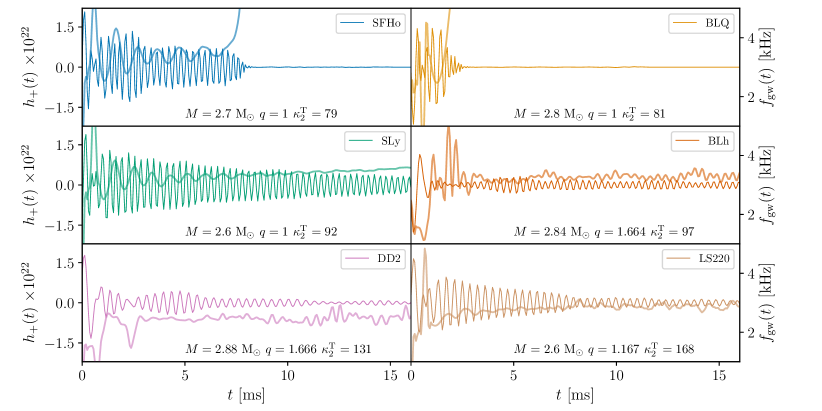
Figure 4: GW signals of the NR validation binaries locating the sources at $D_{L}=100~{}{\rm Mpc}$. The left axes show the plus polarization $h_{+}(t)$ (thin solid lines) and the right axes show the instantaneous GW frequency $f_{\rm gw}(t)$ (thick shadowed lines). The panels focus on the first $16~{}{\rm ms}$ after merger. The time of merger is fixed to $t_{\rm mrg}=0$ for each binary. The signals are sampled with a rate of $16384~{}{\rm Hz}$.

Table 1: Summary of the simulation study performed with NRPMw on NR validation data. The first column reports the morphology of the remnant, i.e. short-lived remnant, long-lived remnant or tidally disrupted remnant. The following seven columns show the NR data properties, i.e. EOS, reference, total mass $M$, mass ratio $q$, tidal polarizability $\kappa^{\rm T}_{2}$, PM peak frequency $f_{2}$ and the time of BH collapse $t_{\rm coll}$. The ninth column report the PM SNR $\rho_{\rm inj}$ of the injected NR data. The remaining columns indicate the median values and the 90% credible regions of the recovered posterior distributions obtained in the injection study averaged over the different noise realizations. The medians and nominal errors for the $\log\mathcal{B}$ are also obtained varying noise realizations and the nominal errors correspond to the maximum and minimum recovered values.

Injected properties

Recovered properties

Morph.

EOS

Ref.

$M$

$q$

$\kappa^{\rm T}_{2}$

$f_{2}$

$t_{\rm coll}$

$\rho_{\rm inj}$

$M$

$q$

$\kappa^{\rm T}_{2}$

$f_{2}$

$t_{\rm coll}$

$\log\mathcal{B}$

$[{\rm M_{\odot}}]$

$[{\rm kHz}]$

$[{\rm ms}]$

$[{\rm M_{\odot}}]$

$[{\rm kHz}]$

$[{\rm ms}]$

Short-lived

SFHo

Bernuzzi et al. (2016)

$2.7$

$1.0$

$79$

$3.42$

$8.0$

7

${3.4}^{+2.2}_{-1.8}$

${1.33}^{+0.59}_{-0.31}$

${318}^{+376}_{-270}$

${2.0}^{+1.7}_{-0.9}$

${21}^{+42}_{-18}$

${3.3}^{+1.6}_{-3.4}$

8

${3.7}^{+1.7}_{-1.7}$

${1.29}^{+0.60}_{-0.22}$

${37}^{+129}_{-29}$

${3.4}^{+0.3}_{-2.0}$

${29}^{+31}_{-24}$

${11.5}^{+1.6}_{-10.1}$

10

${4.3}^{+0.6}_{-1.9}$

${1.13}^{+0.23}_{-0.09}$

${21}^{+73}_{-18}$

${3.41}^{+0.05}_{-0.04}$

${30}^{+28}_{-17}$

${29.8}^{+1.6}_{-12.7}$

BLQ

Prakash et al. (2021)

$2.8$

$1.0$

$81$

$3.44$

$2.7$

7

${3.4}^{+2.0}_{-1.7}$

${1.27}^{+0.66}_{-0.24}$

${233}^{+474}_{-211}$

${2.4}^{+0.7}_{-1.2}$

${23}^{+43}_{-20}$

${4.5}^{+1.5}_{-4.3}$

8

${2.9}^{+1.4}_{-1.2}$

${1.25}^{+0.72}_{-0.21}$

${83}^{+173}_{-73}$

${2.6}^{+0.8}_{-1.1}$

${19}^{+26}_{-17}$

${10.4}^{+1.0}_{-5.2}$

10

${2.6}^{+2.4}_{-0.8}$

${1.17}^{+0.08}_{-0.15}$

${87}^{+174}_{-61}$

${2.65}^{+0.61}_{-0.12}$

${2}^{+35}_{-2}$

${28.5}^{+0.9}_{-4.4}$

Long-lived

SLy

Breschi et al. (2019)

$2.6$

$1.0$

$92$

$3.13$

$21$

7

${4.1}^{+1.6}_{-2.2}$

${1.25}^{+0.59}_{-0.20}$

${217}^{+467}_{-199}$

${2.2}^{+1.3}_{-1.1}$

${34}^{+29}_{-29}$

${2.1}^{+1.5}_{-2.3}$

8

${4.4}^{+1.3}_{-2.3}$

${1.45}^{+0.48}_{-0.36}$

${40}^{+217}_{-33}$

${3.2}^{+0.3}_{-1.9}$

${31}^{+33}_{-22}$

${8.0}^{+1.6}_{-8.2}$

10

${3.4}^{+1.8}_{-0.8}$

${1.20}^{+0.26}_{-0.14}$

${46}^{+58}_{-34}$

${3.26}^{+0.06}_{-0.07}$

${30}^{+33}_{-21}$

${25.5}^{+1.6}_{-9.6}$

LS220

Perego et al. (2019)

$2.6$

$1.167$

$168$

$2.68$

$35$

7

${3.7}^{+2.0}_{-1.5}$

${1.23}^{+0.37}_{-0.22}$

${67}^{+227}_{-55}$

${2.7}^{+0.2}_{-0.2}$

${25}^{+34}_{-18}$

${6.4}^{+1.3}_{-3.7}$

8

${3.9}^{+1.8}_{-1.3}$

${1.30}^{+0.30}_{-0.26}$

${55}^{+95}_{-41}$

${2.67}^{+0.15}_{-0.13}$

${17}^{+27}_{-13}$

${13.9}^{+1.2}_{-4.8}$

10

${3.4}^{+2.3}_{-1.5}$

${1.23}^{+0.32}_{-0.18}$

${70}^{+126}_{-62}$

${2.68}^{+0.12}_{-0.11}$

${18}^{+25}_{-10}$

${33.9}^{+1.4}_{-5.6}$

Tidally disrupted

BLh

Bernuzzi et al. (2020)

$2.84$

$1.664$

$97$

$3.27$

$18$

7

${3.1}^{+2.1}_{-1.2}$

${1.18}^{+0.77}_{-0.17}$

${503}^{+257}_{-436}$

${1.6}^{+1.6}_{-0.7}$

${20}^{+27}_{-18}$

${8.9}^{+1.5}_{-5.3}$

8

${3.2}^{+2.2}_{-1.0}$

${1.17}^{+0.76}_{-0.15}$

${87}^{+195}_{-78}$

${1.5}^{+2.5}_{-0.6}$

${28}^{+24}_{-25}$

${16.6}^{+1.5}_{-5.7}$

10

${3.3}^{+2.3}_{-0.7}$

${1.12}^{+0.81}_{-0.11}$

${62}^{+216}_{-57}$

${1.5}^{+1.9}_{-0.8}$

${19}^{+32}_{-18}$

${38.2}^{+1.6}_{-7.8}$

DD2

$\begin{subarray}{c}\text{This}\\ \text{work}\end{subarray}$

$2.88$

$1.666$

$131$

$2.58$

$34$

7

${3.8}^{+1.8}_{-1.5}$

${1.41}^{+0.52}_{-0.38}$

${261}^{+432}_{-240}$

${1.9}^{+0.9}_{-0.8}$

${20}^{+42}_{-18}$

${5.8}^{+1.5}_{-5.2}$

8

${3.5}^{+1.8}_{-1.4}$

${1.50}^{+0.42}_{-0.47}$

${92}^{+172}_{-73}$

${2.2}^{+0.5}_{-1.1}$

${22}^{+49}_{-20}$

${14.5}^{+1.6}_{-9.0}$

10

${3.3}^{+1.7}_{-1.2}$

${1.63}^{+0.23}_{-0.59}$

${86}^{+130}_{-63}$

${2.13}^{+0.54}_{-0.95}$

${9}^{+31}_{-8}$

${31.8}^{+1.6}_{-12.2}$

In this section, we perform full PE injection-recovery experiments using NR signals and NRPMw; the NR validation set and the main results are summarized in Table 1. The validation set is composed by six non-spinning binaries computed with THC Radice and Rezzolla (2012) which simulate microphysics, neutrino transport (with various schemes) and turbulent viscosity. The set includes two long-lived remnants (SLy with total mass $1.30{+}1.30~{}{\rm M_{\odot}}$ Breschi et al. (2019) and LS220 $1.40{+}1.20~{}{\rm M_{\odot}}$ Perego et al. (2019)), two short-lived remnants (SFHo $1.35{+}1.35~{}{\rm M_{\odot}}$ Bernuzzi et al. (2016) and BLQ $1.40{+}1.40~{}{\rm M_{\odot}}$ Prakash et al. (2021)), and two large-mass-ratio binaries with tidal disruptive morphology (DD2 $1.80{+}1.08~{}{\rm M_{\odot}}$ Breschi et al. (2022b) and BLh $1.772{+}1.065~{}{\rm M_{\odot}}$ Bernuzzi et al. (2020)).

Figure 4 shows the corresponding GW signals from NR simulations. The short-lived SFHo $1.35{+}1.35~{}{\rm M_{\odot}}$ remnant shows prominent modulations around the carrier frequency $f_{2}\simeq 3.4~{}{\rm kHz}$ and increasing frequency drift corresponding to $\alpha_{\rm peak}\simeq 0.075~{}{\rm kHz}^{2}$. The remnant collapses at $t_{\rm coll}\simeq 8~{}{\rm ms}$. The second short-lived case, BLQ $1.40{+}1.40~{}{\rm M_{\odot}}$, is computed with an EOS that includes a deconfined quark phase. The remnant collapses into a BH shortly after the first bounce of the core collision, at $t_{\rm coll}\simeq 3~{}{\rm ms}$, and the corresponding $f_{2}\simeq 3.4~{}{\rm kHz}$ peak deviates from the quasiuniversal relation above the $90\%$ credibility region (see Paper I). Moreover, for this binary, it is not possible to estimate the frequency drift parameter $\alpha_{\rm peak}$ since the remnant collapses before the third nodal point (see Paper I, for the definition of $\alpha_{\rm peak}$ and nodal points). The long-lived SLy $1.30{+}1.30~{}{\rm M_{\odot}}$ remnant shows prominent modulations around the carrier frequency $f_{2}\simeq 3.1~{}{\rm kHz}$ with $\alpha_{\rm peak}\simeq 0.032~{}{\rm kHz}^{2}$ and collapses into a BH $21~{}{\rm ms}$ after merger. The second long-lived remnant, LS220 $1.40{+}1.20~{}{\rm M_{\odot}}$, survives $35~{}{\rm ms}$ after merger, and its spectrum peaks at $f_{2}\simeq 2.7~{}{\rm kHz}$. For times $\lesssim 20~{}{\rm ms}$ after merger, the corresponding GW PM signal shows an increasing frequency evolution with $\alpha_{\rm peak}\simeq 0.027~{}{\rm kHz}^{2}$; however, the instantaneous frequency decays during the final stages with $\alpha_{\rm peak}\simeq-0.037~{}{\rm kHz}^{2}$. Averaging over the entire PM duration, we estimate an $\alpha_{\rm peak}$ of $-0.01~{}{\rm kHz}^{2}$. The tidal disruptive BLh $1.772{+}1.065~{}{\rm M_{\odot}}$ remnant collapses into a BH $18~{}{\rm ms}$ after merger, and it corresponds to the intrinsically fainter PM GW signal of our set. The frequency evolution is milder compared to the previous cases, with $\alpha_{\rm peak}\simeq 0.015~{}{\rm kHz}^{2}$ and its spectrum shows $f_{2}\simeq 3.3~{}{\rm kHz}$ with multiple subdominant peaks. The second tidal disruptive case, DD2 $1.80{+}1.08~{}{\rm M_{\odot}}$, generates a remnant that collapses $34~{}{\rm ms}$ after merger and it approximately shows a constant frequency evolution, $\alpha_{\rm peak}\simeq 5{\times}10^{-3}~{}{\rm kHz}^{2}$. The corresponding spectrum shows PM peak centered around ${\sim}2.6~{}{\rm kHz}$.

In Sec. IV.1 we investigate the signal detectability as a function of the injected SNR of the NR data. We discuss the posterior distributions for the spectra in Sec. IV.2 and for the characteristic PM frequencies in Sec. IV.3. Then, we present the obtained constraints on binary parameters (Sec. IV.4) and the PM parameters (Sec. IV.5).

IV.1 Detectability

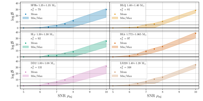
Figure 5: Logarithmic BFs $\log\mathcal{B}$ as functions of the PM SNR $\rho_{\rm inj}$ of the injected NR template from Table 1. The dots refer to the mean values averaged over the different noise realizations and the shadowed areas correspond to the minimum and maximum values recovered in the survey. Two horizontal lines identify $\log\mathcal{B}=0$ (black) and $\log\mathcal{B}=5$ (gray).

Figure 5 shows the recovered mean, maximum and minimum BFs for the binaries listed in Table 1. In general, the BFs show the expected increasing trend deviating from $\log\mathcal{B}\simeq 0$ and recovering informative posterior distributions at PM SNR $\rho_{\rm inj}\simeq 6$. Averaging over all the analyzed cases, the nominal detectability threshold is reached for PM SNR $\rho_{\rm inj}=7.2^{+0.8}_{-0.5}$. Noise fluctuations affect the estimates, leading to larger threshold SNRs similarly to the analysis of Sec. III.1, but with more pronounced and less homogeneous fluctuations. The recovered BFs for the binaries with $\kappa^{\rm T}_{2}\lesssim 90$ have a slower trends compared with the other cases and the case-study of Sec. III, showing $\log\mathcal{B}\lesssim 30$ for SNR 10. The corresponding PM transients show the most significant modulation effects among the considered cases and a short duration, except for SLy $1.30{+}1.30~{}{\rm M_{\odot}}$. Moreover, the characteristic PM peaks for these cases are located at higher frequency values compared to the other binaries, i.e. $f_{2}\gtrsim 3~{}{\rm kHz}$, where the noise contributions increase. The detectability threshold for these cases could be improved by a refined characterization of the frequency modulations (e.g. introducing a free modulation phase as a free parameter), or refining the late-time portion of the template (e.g. including the wavelet for the BH collapse).

IV.2 Spectra

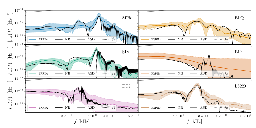
Figure 6: Posterior distributions of the GW spectra for the PMs plus polarization $h_{+}(f)$ recovered for PM SNR $\rho_{\rm inj}=10$ for an illustrative noise realization. The colored lines report the medians and the shadowed regions correspond to the 90% credibility region. The injected spectra are reported with black solid lines and the corresponding $f_{2}$ peaks are denoted with vertical black dotted lines.

Figure 6 shows the posterior distribution of the recovered spectra for an illustrative noise realization at $\rho_{\rm inj}=10$. We opt to report this case because it corresponds to the loudest employed SNR and therefore the systematic errors between NRPMw model and NR data are more evident. In general, the majority of the injected signals are included within the 90% confidence levels of the recovered spectra, consistently with the discussion on the recovered SNRs of Sec. IV.1.

The large mass ratio binaries BLh and DD2 underestimate the characteristic PM peak. In particular, the predicted spectra for the BLh case is primarily informed by the merger portion of data. and it strongly deviates from the injected value due to the faint PM burst, that does not permit a clear identification of the dominant PM peak. The 90% confidence level of the recovered time-domain waveform shows a non-vanishing tail for late times; however, the median value is consistent with zero, showing that the signal is not resolved. These errors can be related with a non-optimal modeling for large mass ratios, i.e. $q>1.5$. In particular, tidally-disruptive mergers show additional phase discontinuities and multiple bumps in the time-domain GW amplitude, related with the remnant dynamics.

IV.3 PM frequencies

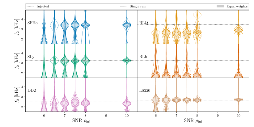
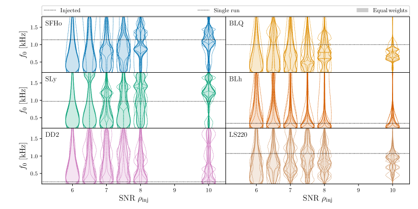
Figure 7: Posterior distributions for the PM frequencies $f_{2}$ (top panel) and $f_{0}$ (bottom panel) at the different PM SNR $\rho_{\rm inj}$ recovered in the PE survey reported in Tab. 1. For each case, thin dashed lines report the recovered posteriors for each run and the filled areas show the equally-weighted combined posterior distributions. Black horizontal dotted lines indicate the values of the injected NR templates.

In NRPMw, the actual $f_{2}$ value is determined by several quantities. A first estimate relies on the binary parameters through the quasiuniversal relation. Then, the frequency drift parameter $\alpha_{\rm peak}$ and the value of the respective recalibrations ${\boldsymbol{\delta}_{\rm fit}}$ can shift the actual peak from the prediction of the quasiuniversal relation. Thus, a robust determination of the PM frequency can be estimated from the peak of the reconstructed spectra, consistently with the extraction method discussed in Sec. 4 B of Paper I. For each sample, we generate the corresponding GW spectrum $h_{{\tt NRPMw}}(f)$, considering only the time support $t>t_{0}$ in order to isolate the PM contribution of interest. Then, $f_{2}$ is identified as the (typically dominant) spectral peak of the carrier frequency component. When the template corresponds to prompt BH collapse, a prior sample is extracted.

Figure 7 (top panel) shows the recovered posterior distributions on $f_{2}$ as a function of the injected SNR $\rho_{\rm inj}$. As mentioned in the previous section, for the majority of the cases the recovered posteriors report informative inferences for $\rho_{\rm inj}\gtrsim 6$ with errors of $O(1~{}{\rm kHz})$. The errors on the estimated $f_{2}$ decrease to $O(100~{}{\rm Hz})$ at PM SNR 10. These results are comparable with similar estimates performed with unmodeled studies Chatziioannou et al. (2017) and strongly improve the results coming from damped-sinusoidal templates Tsang et al. (2019); Easter et al. (2020). Template-based analyses are expected to deliver better detectability threshold than model-independent estimates, if the employed template is a good representation of the signal. Thus, in this perspective, this claim might appear counterintuitive. However, template-based studies of PM transients are generally showing poorer results than the more flexible models due to the considerable mismatch between the employed template and the signal. In NRPMw, these biases are corrected with the recalibration $\boldsymbol{\delta}_{\rm fit}$, accounting for deviations from the predictions of the calibrated relations. At SNR $\rho_{\rm inj}=8$, all posterior distributions show informative measurements, with uncertainties ranging from $1~{}{\rm kHz}$ to $500~{}{\rm Hz}$, and the injected NR values are included in the $90\%$ credible regions. The uncertainties on the $f_{2}$ posteriors reach $O(100~{}{\rm Hz})$ at SNR $\rho_{\rm inj}=10$ and systematic uncertainties start to play a more significant role. In particular, the analyses of the short-lived remnant BLQ show bimodalities in the $f_{2}$ posteriors for some noise realizations. These biases are attributable to subdominant couplings that have a larger contribution on the overall spectrum for short-lived remnants, whose power can exceed that of the $f_{2}$ peak (see Fig. 6). Similar biases are recovered also in the analysis of the DD2 binary. On the other hand, as discussed in Sec. IV.2, the inference of the BLh binary is not capable to resolve the $f_{2}$ peak.

Another interesting quantity is the coupling frequency $f_{0}$. This component induces a modulation in of the carrier frequency $f_{2}$, generating the subdominant spectral peaks, especially for very compact remnants . The $f_{0}$ frequency is generally related with mass-density oscillations of the NS remnant; thus, it can provide important insights on the NS structure (e.g. Stergioulas et al., 2004; Bernuzzi and Nagar, 2008; Bernuzzi, 2009; Radice et al., 2010; Stergioulas et al., 2011). We estimate the $f_{0}$ posterior from the instrinsic binary properties employing the quasiuniversal relations and modifying the prediction with the associated recalibration parameter $\delta_{f_{0}}$. Differently from $f_{2}$, the actual values of $f_{0}$ is fully determined by these quantities since NRPMw assumes this frequency component to be constant. Figure 7 (bottom panel) shows the recovered posterior distributions on $f_{0}$ as a function of the injected SNR $\rho_{\rm inj}$. The recovered $f_{0}$ posteriors are generally broader than the $f_{2}$ ones, due to the weaker magnitude of these spectral peaks. The results show informative measurements for PM SNR $\gtrsim 7.5$ with errors of $O(1~{}{\rm kHz})$. The uncertainties decrease to $O(500~{}{\rm Hz})$ at PM SNR 10. Moreover, noise fluctuations affect $f_{0}$ posterior introducing biases and multimodalities due to the weakness of the associated spectral peaks.

IV.4 Binary parameters

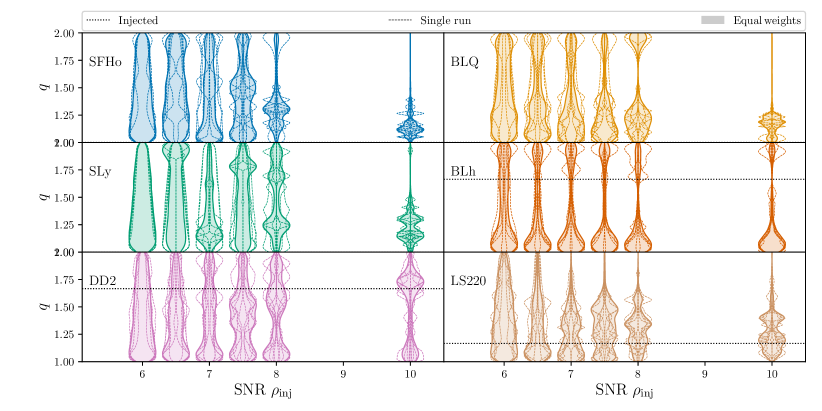
Figure 8: Posterior distributions for the mass ratio $q$ (top panel) and the tidal polarizability $\kappa^{\rm T}_{2}$ (bottom panel) at the different PM SNR $\rho_{\rm inj}$ recovered in the PE survey reported in Tab. 1. For each case, thin dashed lines report the recovered posteriors for each run and the filled areas show the equally-weighted combined posterior distributions. Black horizontal dotted lines indicate the values of the injected NR templates.

The intrinsic binary parameter are generally poorly constrained compared to the pre-merger analysis due to the considerably smaller SNR of the PM signal. Overall, the recovered posteriors show a behavior similar to the case discussed in Sec. III. The median binary masses $M$ are typically shifted toward larger values, with errors of $O(1~{}{\rm M_{\odot}})$. Nevertheless, the injected values are always included in the $90\%$ credible regions, indicating that our inference is unbiased at the SNRs under consideration. The mass ratio, shown in Fig. 8 (top panel), is typically well identified up to PM SNR ${\sim}8$ with errors of ${\sim}0.6$ at sensitivity threshold. For increasing SNRs, systematic errors become more dominant especially for equal-mass binaries, where the overall PM power is larger. The tidal polarizability $\kappa^{\rm T}_{2}$ shows systematic errors for PM SNR$~{}\gtrsim 8$, underestimating the injected values, consistently with the mass biases and analogously to the studies in Sec. III. However, as shown in Fig. 8 (bottom panel), the average over the different noise realizations mitigates the systematic biases, including the injected values within the 90% credibility region for all considered binaries. The spins are generally dominated by the prior up to PM SNR ${\sim}10$.

Comparing these results with the ones in Ref. Breschi et al. (2019), we observe an overall widening of the posterior distributions, which is related to the inclusion of the recalibrations ${\boldsymbol{\delta}_{\rm fit}}$. However, at the same time the systematic biases are considerably reduced, showing that such technique is able to providing accurate and conservative results. The obtained results are consistent with the estimates of Ref. Breschi et al. (2022a).

IV.5 PM parameters

Figure 9: Posterior distributions for the time of collapse $t_{\rm coll}$ (top panel) and the frequency drift $\alpha_{\rm peak}$ (bottom panel) at the different PM SNR $\rho_{\rm inj}$ recovered in the PE survey reported in Tab. 1. For each case, thin dashed lines report the recovered posteriors for each run and the filled areas show the equally-weighted combined posterior distributions. Black horizontal dotted lines indicate the values of the injected NR templates. In the BLQ case, extracting a prediction was not possible (see main text).

Figure 9 (top panel) shows the posterior distributions for the time of BH collapse $t_{\rm coll}$ as functions of the injected SNR. This term is strongly affected by noise fluctuations, since the late-time signal tail is no more observable when its amplitude goes below the noise threshold. However, the injected values are generally included within the 90% confidence levels. The associated uncertainties go from $O(30~{}{\rm ms})$ at threshold SNR to $O(20~{}{\rm ms})$ at PM SNR 10. A particular case is the BLQ binary that corresponds to the most massive binary with the shortest PM transient among the considered cases. The corresponding posterior distribution for SNR 10 is tightly constrained around the injected value, implying that $t_{\rm coll}$ can be better estimated for very-short-lived remnants. The inference of $t_{\rm coll}$ can be improved introducing the model for the remnant collapse in NRPMw (see Paper I). However, the observation of the BH collapse is strongly limited by the sensitivity of the detectors at the corresponding BH frequencies, that occur at $f\gtrsim 6~{}{\rm kHz}$ for typical BNS systems.

Figure 9 (bottom panel) shows the posterior distributions for the frequency drift $\alpha_{\rm peak}$ as functions of the injected SNR. Differently from $t_{\rm coll}$, this term appears to be better constrained for long-lived equal-mass binaries. This is due to the nature of these PM GW transients. In fact, their spectra are characterized by the loudest PM peaks, permitting an improved identification of the peak properties compared to the short-lived remnant cases. Also $\alpha_{\rm peak}$ is affected by noise fluctuations, affecting primarily the widths of the recovered posteriors. However, for SNR $\gtrsim 10$, systematic errors become more relevant. A particular case is LS220 binary, for which the recovered posterior overestimates the nominal injected value. However, as previously discussed, this case has non-monotonic frequency evolution. Thus, NRPMw is recovering the initial slope of the LS220 transient, corresponding to the loudest contribution. For unequal-mass binary, $\alpha_{\rm peak}$ is poorly constrained due to the faintness of the late-time portion of the GW transient.

V EOS softening tests

Figure 10: Posterior distributions of the recovered spectra for the DD2 (blue) and the BHB$\Lambda\phi$ (red) binaries at PM SNR 8. The solid colored lines report the median spectrum and the contours show the 90% credible regions. The black solid lines correspond to the injected signals and black dotted lines correspond to the $f_{2}$ peak. The green lines show the amplitude spectra density (ASD). The gray lines show the artificial data.

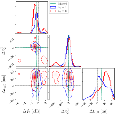
Figure 11: Posterior distribution for the deviations $\{\Delta f_{2},\Delta\kappa^{\rm T}_{2},\Delta t_{\rm coll}\}$ between the DD2 and the BHB$\Lambda\phi$ analyses for PM SNR 8 (blue) and 10 (red). The contours correspond to the 50% annd 90% credibility regions. The injected deviations are reported with green dashed lines and the zero hypothesis is reported with black dotted lines. A deviation is defined as $\Delta Q=Q^{\rm DD2}-Q^{{\rm BHB}\Lambda\phi}$ for each quantity $Q$.

In this Section, we study the possibility of inferring an EOS softnening from a detection of PM signal. Specifically, we repeat the analysis presented in Sec. V D of Breschi et al. (2019) with the updated model NRPMw and employing ET detector. The injections are performed within the same framework discussed in Sec. II with PM SNR $\rho_{\rm inj}=\{8,10\}$ using a single noise realization. We perform PE on the PM transients solely; the latter are computed from NR simulations of $1.50{+}1.50~{}{\rm M_{\odot}}$ BNS systems described by DD2 and BHB$\Lambda\phi$ EOSs Radice et al. (2017). The two EOSs are identical except for the inclusion of hyperonic degrees of freedom at high densities in BHB$\Lambda\phi$ Banik et al. (2014). This inclusion introduces a softening at the extreme densities reached in the remnant and deviates from DD2 at typical densities $\rho\simeq 2\rho_{\rm sat}$, where $\rho_{\rm sat}=2.7{\times}10^{14}~{}{\rm g}~{}{\rm cm}^{-3}$ is the nuclear saturation density. The main question we address is whether an analysis of PM signal can inform us on the EOS softening effects at extreme densities, and what are the most relevant quantities that indicate the softening.

Previous studies performed with NRPM showed that the $f_{2}$ posterior of the BHB$\Lambda\phi$ strongly differs from the DD2 case Breschi et al. (2019). We remark that the DD2 $1.50{+}1.50~{}{\rm M_{\odot}}$ binary has $f_{2}\simeq 2.76~{}{\rm kHz}$; while, the respective BHB$\Lambda\phi$ case has $f_{2}\simeq 3.29~{}{\rm kHz}$ . The difference between the two NR values is ${\sim}500~{}{\rm Hz}$, which corresponds to ${\sim}15\%$. The BHB$\Lambda\phi$ data deviates of ${\sim}3{-}\sigma$ from the prediction of the EOS-insensitive relation presented in Paper I ($f_{2}^{\rm fit}=2.88~{}{\rm kHz}$), encoding a more compact remnant than the DD2 case. The two binaries have also different times of BH collapse: the DD2 case collapses at late times, i.e. $t_{\rm coll}\simeq 21~{}{\rm ms}$; while, the BHB$\Lambda\phi$ remnant collapses into BH shortly after merger with $t_{\rm coll}\simeq 2.6~{}{\rm ms}$. The BHB$\Lambda\phi$ $1.50{+}1.50~{}{\rm M_{\odot}}$ binary shows the largest deviations from the quasiuniversal fits used in NRPMw.

The spectra recovered in the new analyses performed with NRPMw at PM SNR 8 are shown in Fig. 10. The recovered SNRs are consistent with the injected values, recovering $\rho_{\rm rec}={7.5}^{+1.0}_{-1.4}$ and a BF $\log\mathcal{B}=6.3\pm 0.2$ for the DD2 case; while, for the BHB$\Lambda\phi$, we get $\rho_{\rm rec}={7.4}^{+1.2}_{-1.2}$ and $\log\mathcal{B}=6.5\pm 0.2$. The posterior distributions for the intrinsic binary parameters do not show significant differences between the two cases. This is key in view of coherent and informative consistency tests  (e.g. Breschi et al., 2019; Wijngaarden et al., 2022). We recover $M\simeq 4.3~{}{\rm M_{\odot}}$ with an error of ${\sim}1.5~{}{\rm M_{\odot}}$. The mass ratios are constrained around the equal-mass case with errors of ${\sim}0.25$. The tidal polarizability $\kappa^{\rm T}_{2}$ underestimates the injected values with medians $\kappa^{\rm T}_{2}\simeq 30$ and errors ${\sim}150$. The spins posteriors are dominated by the priors and not informative.

At SNR 8, the $f_{2}$ posteriors show different median values corresponding to $f_{2}={2.73}^{+0.05}_{-0.06}~{}{\rm kHz}$ for DD2 and $f_{2}={3.2}^{+0.9}_{-1.0}~{}{\rm kHz}$ for BHB$\Lambda\phi$. The difference between the recovered $f_{2}$ exceed the $1{-}\sigma$ credibility level of the $f_{2}$ EOS-insensitive relation, highlighting a breaking of quasiuniversality within that level. This deviation is partially encoded in the related recalibration parameters that recovered opposite values, i.e. $\delta_{f_{2}}={-1}^{+7}_{-4}~{}\%$ for DD2 and $\delta_{f_{2}}={2}^{+6}_{-9}~{}\%$ for BHB$\Lambda\phi$. In this context, the inclusion of the recalibration coefficients is crucial since they allow the observed PM peak to deviate from the prediction of the quasiuniversal relation for a common combination of intrinsic binary parameters. However, the short duration of the BHB$\Lambda\phi$ transient and the strong modulations can introduce biases and multimodalities in the estimates of the associated peak frequency, as also shown in the analysis of the BLQ binary in Sec. IV.

Another quantity that encodes the softening of the EOS at high densities is the time of BH collapse $t_{\rm coll}$. A softer EOS allows the NS remnant to reach higher densities, yielding to an earlier BH collapse for comparable masses Radice et al. (2017); Prakash et al. (2021); Fujimoto et al. (2022). The recovered posteriors at SNR 8 for $t_{\rm coll}$ give $t_{\rm coll}={28}^{+36}_{-24}~{}{\rm ms}$ for DD2 and $t_{\rm coll}={6}^{+41}_{-4}~{}{\rm ms}$ for BHB$\Lambda\phi$, consistently with the injected values. Even if this term can be strongly affected by noise fluctuations at low SNRs, as discussed in Sec. IV.5, the estimate of $t_{\rm coll}$ appears to be less biased and more conservative compared to the $f_{2}$ one. Moreover, the $t_{\rm coll}$ posterior is expected to converge to the true value for increasing SNR for short-lived remnant, as shown by the BLQ binary in Sec. IV. Thus, the measurement of $t_{\rm coll}$ is expected to be a robust probe of softening effects in the NS EOS for PM SNR $\gtrsim 9$.

In order to validate the robustness of the inference, we repeat the analysis injecting the signals at PM SNR 10. The recovered SNRs are $\rho_{\rm rec}={7.8}^{+1.2}_{-1.2}$ and $\log\mathcal{B}=7.0\pm 0.2$ for the DD2 case and $\rho_{\rm rec}={7.6}^{+1.8}_{-1.9}$ and $\log\mathcal{B}=9.6\pm 0.2$ for the BHB$\Lambda\phi$ case. The dominant systematic appears in the $f_{2}$ posterior distribution for BHB$\Lambda\phi$. This posteriors shows pronounced multimodalities due to the contribution of the subdominant coupled frequencies $f_{2\pm 0}$, as discussed previously. The median values and the $90\%$ credibility intervals correspond to $f_{2}={2.75}^{+0.03}_{-0.03}~{}{\rm kHz}$ for the DD2 binary and $f_{2}={3.7}^{+0.3}_{-2.7}~{}{\rm kHz}$ for the BHB$\Lambda\phi$ binary. The $t_{\rm coll}$ posterior distributions show convergent trends toward the injected values for both cases, recovering $t_{\rm coll}={54}^{+5}_{-41}~{}{\rm ms}$ for the DD2 binary and $t_{\rm coll}={16}^{+11}_{-13}~{}{\rm ms}$ for the BHB$\Lambda\phi$ binary. From these results, it is possible to understand that the short-lived binaries (such as the BHB$\Lambda\phi$ case) show more ambiguous $f_{2}$ posteriors and more informative $t_{\rm coll}$ posteriors for increasing SNRs. On the other hand, for the long-lived binaries (such as the DD2 case), the $f_{2}$ posterior is typically unbiased and the $t_{\rm coll}$ posterior is more affected by noise fluctuations, but showing convergence toward the injected value and typically including the latter within the 90% credibility intervals.

Aiming to highlight the differences between the DD2 and BHB$\Lambda\phi$ posterior distributions, we introduce the deviation $\Delta Q=Q^{\rm DD2}-Q^{{\rm BHB}\Lambda\phi}$, where $Q$ is an arbitrary PM quantity. Figure 11 shows the posterior distributions for $\{\Delta f_{2},\Delta\kappa^{\rm T}_{2},\Delta t_{\rm coll}\}$ for the analyses with SNR 8 and 10. In a realistic scenario, such computation is unlikely since it would require the observation of two identical BNS mergers with different EOS. However, in order to understand the performances of the model, this representation clearly evinces the differences between the recovered posteriors. The $\Delta f_{2}$ posterior reports mild deviations for SNR 8, i.e. $\Delta f_{2}={-0.5}^{+1.0}_{-0.9}~{}{\rm kHz}$; while, for SNR 10, the average deviation increases, i.e. $\Delta f_{2}={-0.9}^{+2.6}_{-0.9}~{}{\rm kHz}$, but the posterior introduces ambiguities due to multimodalities. The $\Delta\kappa^{\rm T}_{2}$ posteriors confidently include the zero hypothesis within the support and it shows small multimodalities due to the correlation with the PM frequency $f_{2}$ at SNR 10. On the other hand, the $\Delta t_{\rm coll}$ posteriors show unambiguous convergence toward a non-zero value for increasing SNR. The median values and the 90% credibility intervals are $\Delta t_{\rm coll}={16}^{+46}_{-44}~{}{\rm ms}$ at SNR 8 and $\Delta t_{\rm coll}={35}^{+23}_{-42}~{}{\rm ms}$ at SNR 10.

VI Conclusions

We presented PE studies on PM GW transients solely from BNS merger remnants with the novel template model NRPMw focusing on next-generation detector ET Hild et al. (2011); Hild (2012). Performing a survey of $245$ PE studies with seven different artificial templates and five noise realizations, we demonstrated that ET can detect PM signals from a threshold SNR ${\sim}7$ using NRPMw template and without any pre-merger information. These SNRs correspond to (optimally-oriented) binaries located at luminosity distances of ${\sim}100~{}{\rm Mpc}$, that are values consistent with recent observations of BNS mergers Abbott et al. (2020). Employing estimates of BNS merger rates Abbott et al. (2021), we compute an upper limit of ${\sim}4$ observable BNS mergers per year in a spherical volume of radius $100~{}{\rm Mpc}$.

The inference with the novel NRPMw improves over the previous NRPM Breschi et al. (2019, 2022a) due to the improved calibration of EOS-sensitive relations performed in Paper I. The inference results are consistent with the expectations from the faithfulness studies reported in Paper I. We have shown that NRPMw can provide constraints on several characteristic properties of the observed PM signals. The uncertainties on the $f_{2}$ posteriors are $O(1~{}{\rm kHz})$ at PM SNR 7 and $O(100~{}{\rm Hz})$ at PM SNR 10. However, systematic errors arise for short-lived and large-mass-ratio remnants for SNR $\gtrsim 8$ primarily related to an inaccurate identification of the characteristic PM peak. The time of BH collapse $t_{\rm coll}$ can be estimated with an accuracy of $O(20~{}{\rm ms})$ at PM SNR 10. The inference of this term is significantly affected by the employed noise realization, since the late-time tail of the PM signal is masked by noise fluctuations. Moreover, NRPMw can provide measurements of the subdominant coupling frequency $f_{0}$, of the frequency drift $\alpha_{\rm peak}$ and on the intrinsic BNS properties; however, the latter appears to be generally poorly constrained compared to a corresponding pre-merger analysis (e.g. Breschi et al., 2019; Wijngaarden et al., 2022).

Our injection survey with NRPMw indicates that the largest biases and systematic errors arise for very-short-lived remnants and tidally-disruptive mergers. These errors are primarily related to misinterpretation of the subdominant coupling frequencies or to an insufficient GW power in the PM segment. The systematic biases can be mitigated improving the model morphology in the large-mass-ratio regimes, when more NR simulations become available, and including the wavelet corresponding to the BH ringdown (see Paper I). However, a full description of the PM collapse dynamics in BNS mergers will require a more accurate characterization and modeling, in particular for large-mass-ratio mergers, i.e. $q>1.5$, and massive remnants, i.e. $M\gtrsim 2.8~{}{\rm M_{\odot}}$. Nevertheless, the direct observation of the BH collapse and the subsequent ringdown radiation are considerably limited by the detector sensitivities in these extreme region of the Fourier spectrum, i.e. $f\gtrsim 6~{}{\rm kHz}$. Thus, a neat observation of a BH ringdown after a BNS merger is challenging.

PM signals can, in principle, inform us on the appearance of non-nucleonic degrees of freedom at extreme matter densities. A possible imprint of a EOS softening in the signal is the breaking of the quasiuniversal relations that characterize the spectral features. For example, several NR simulations indicate that deviations of the orders of ${\sim}500~{}{\rm Hz}$ in the $f_{2}$ peak and of ${\sim}20~{}{\rm ms}$ in the time of BH collapse are possible due EOS softening, (e.g. Sekiguchi et al., 2011; Radice et al., 2017; Bauswein et al., 2019; Prakash et al., 2021; Fujimoto et al., 2022). We considered a short-lived remnant as a case study and demonstrate that ${\sim}3{-}\sigma$ violations of EOS-insensitive relations are potentially observable at PM SNR 8. However, the short duration of the PM transient might lead to biases in the inference of $f_{2}$ for SNR $\gtrsim 9$. On the other hand, the inference of the time of collapse $t_{\rm coll}$ delivers more robust measurements for increasing SNRs for short-lived remnant. We stress that the breaking of a quasiuniversal relation within a given confidence level does not necessarily imply the presence of an EOS softening . Instead, more generally, such a breakdown should be interpreted as the invalidation of a particular empirical relation due to physical effects that not captured by the constructed fit. Similarly, a EOS softening might break a quasiuniversal relation only in a marginally significant way, as in our case study, or the remnant’s densities might be such that these effects are not evident, e.g. small mass binaries $M\ll 3~{}{\rm M_{\odot}}$ Radice et al. (2017); Prakash et al. (2021). In the future, it would be interesting to verify the performances of NRPMw against NR templates computed with more extreme EOS that show larger deviations from the quasiuniversal trends (e.g. Bauswein et al., 2019; Wijngaarden et al., 2022). In general, more accurate studies of BNS merger with non-nucleonic EOS, driven by high-precision NR simulations (e.g. Radice et al., 2017; Prakash et al., 2021; Fujimoto et al., 2022), are essential in order to comprehensively characterize to what extend the breaking of EOS-insensitive relations can probe EOS softening.

Finally, our results should be revisited with a full inspiral-merger-postmerger analysis, similarly to what presented in Ref. Breschi et al. (2019); Wijngaarden et al. (2022). These studies will be reported in the third paper of this series. The pre-merger information is expected to provide narrower constraints on the intrinsic binary parameters and to reduce the related biases Breschi et al. (2019); Wijngaarden et al. (2022). This will have a significant effects on the overall inference, e.g. improving the identification of the correlations between the intrinsic and the PM parameters. Moreover, the recalibration parameters are expected to have a more relevant effect on the recovered posteriors, highlighting more noticeable deviations from quasiuniversal behavior. The pre-merger information will also contribute to the inference high-density EOS properties Breschi et al. (2022a) and to the identification of softening effects, allowing coherent pre-and-post-merger consistency tests Breschi et al. (2019).

References

- Hild et al. (2008) S. Hild, S. Chelkowski, and A. Freise, (2008), arXiv:0810.0604 [gr-qc] .
- Radice et al. (2020) D. Radice, S. Bernuzzi, and A. Perego, Ann. Rev. Nucl. Part. Sci. 70 (2020), 10.1146/annurev-nucl-013120-114541, arXiv:2002.03863 [astro-ph.HE] .
- Bernuzzi (2020) S. Bernuzzi, Gen. Rel. Grav. 52, 108 (2020), arXiv:2004.06419 [astro-ph.HE] .