Input estimation from discrete workload observations in a Lévy-driven storage system

Abstract

We consider the estimation of the characteristic exponent of the input to a Lévy-driven storage model. The input process is not directly observed, but rather the workload process is sampled on an equispaced grid. The estimator relies on an approximate moment equation associated with the Laplace-Stieltjes transform of the workload at exponentially distributed sampling times. The estimator is pointwise consistent for any observation grid. Moreover, the distribution of the estimation errors is asymptotically normal for a high frequency sampling scheme. A resampling scheme that uses the available information in a more efficient manner is suggested and studied via simulation experiments.

Keywords. Lévy-driven storage system $\circ$ Statistical inference $\circ$ Discrete workload observations $\circ$ High-frequency sampling

Acknowledgments. The research of Michel Mandjes Liron Ravner is partly funded by NWO Gravitation project Networks, grant number 024.002.003.

1 Introduction

To optimally design and control queueing systems, it is of crucial importance to have reliable estimates of model primitives. One important class of such systems is formed by so called Lévy-driven queues, see e.g. Dębicki and Mandjes, (2015), which can be regarded as Lévy processes on which the Skorokhod map is imposed (or, equivalently, Lévy processes reflected at $0$). A Lévy process is uniquely characterized by its Lévy exponent, a function that captures a full probabilistic description of the process dynamics. This paper deals with estimation of the Lévy exponent from equidistant observations of the reflected process. Within the broad class of Lévy-driven queues, we focus on storage systems whose input is a non-decreasing Lévy process. A special case of the last type of systems is the classical M/G/1 queue, where the driving Lévy process is a compound Poisson process.

When it comes to estimation of model primitives in the setting of Lévy-driven queues, a main complication is that in many situations one cannot observe the queue’s input process (in the concrete case of the M/G/1 queue: the individual interarrival times and service requirements); instead, one often only has discrete equidistant observations of the associated workload process. The challenge lies in developing sound techniques to statistically estimate, based on these workload observations, the Lévy exponent corresponding the system’s input process. This type of inverse problem is not straightforward because densities are unavailable, impeding the use of conventional maximum likelihood procedures. Ravner et al., (2019) constructed a method of moments estimator for the Lévy exponent of the input process by sampling the workload according to an independent Poisson process. The advantage of so-called Poisson sampling is that the distribution of the workload after an exponentially distributed time conditional on an initial workload is known, in terms of the Laplace-Stieltjes transform (LST). This paper shows that the Poisson sampling framework can be leveraged to construct estimators for the Lévy exponent even when the sampling times are deterministic and not random.

Approach and main contributions

The main contribution of this paper is the construction of an estimator of the Lévy exponent of the queue’s input process, based on discrete equidistant workload observations. Note that this is a challenging task even for the special case of compound Poisson input (M/G/1) because of the intractable underlying transient dynamics of the workload process. The suggested estimator relies on an approximate moment equation associated with the Laplace-Stieltjes transform of the workload at exponentially distributed sampling times. It can be considered as an approximate method of moments estimator, since it is derived from a moment equation which, due to discretization, is not exact. As mentioned above, the approximate estimation equation relies on the Poisson sampling scheme of Ravner et al., (2019). However, their estimator, and associated asymptotic results, relied on an intermediate step of estimating the inverse of the Lévy exponent at the point of the Poisson sampling rate. We provide a slightly modified estimation equation that no longer requires this intermediate step. On top of the practical and computational advantages of this direct method, this further enables a simpler derivation of the asymptotic variance of the estimation error (for both the Poisson and high-frequency equidistant sampling schemes).

We further provide performance guarantees of the estimator. In the first place we establish consistency, which, remarkably, is not affected by the ‘grid width’ $\Delta$ (i.e., the time between two subsequent observations). We then prove asymptotic normality, which requires us to pick $\Delta$ in a specific way, depending on the number of observations $n$; the underlying argumentation distinguishes between the case that the driving Lévy process is of finite and infinite intensity. Finally, we propose a resampling scheme that uses the available information in a more efficient manner. Simulation experiments demonstrate its efficacy.

Related literature

An exhaustive recent overview of the existing statistical queueing literature is given in Asanjarani et al., (2021). Here we restrict ourselves to discussing the results that directly to our work. It is important to stress that the various models considered differ in terms of the width of the class of input processes (e.g. compound Poisson versus Lévy) and the nature of the observations (e.g. workload at Poisson instants versus workload at equidistant instants, and the ‘degree of partial information’).

A closely related paper is Hansen and Pitts, (2006), describing a non-parametric approach for the M/G/1 queue. The authors use the empirical cumulative distribution function (ecdf) of the periodically sampled workload to estimate the traffic intensity and the service time distribution. Among the results are central limit theorems (CLTs) for the ecdf of the workload and residual service time. The work of Basawa et al., (1996) discusses a maximum likelihood estimator based on the waiting times of the customers in a GI/G/1 queue, that is, observations from the workload process just prior to the arrivals, the main result here also being a CLT. Another stream of the literature focuses on nonparametric estimation of the input distribution to infinite server queueing systems; these systems have the intrinsic advantage that clients do no wait, which is, for estimation purposes, a convenient feature. For example, Bingham and Pitts, (1999) and Goldenshluger, (2016) suggest estimators (and provide corresponding performance guarantees) based on observations of the number of clients present.

Outside the context of queueing systems, there is substantial literature on estimation of Lévy processes. Here, having discrete observations (of the process’ increments, that is) is also a common assumption. For references in this area, we refer to for example van Es et al., (2007), Kappus and Reiß, (2010), Belomestny and Reiß, (2015) and references therein.

No statistical methods had been proposed in the setting of storage system with Lévy input, until the appearance of Ravner et al., (2019). This reference, that can be considered as a precursor to the present paper, suggests an estimator of the Lévy exponent based on workload observations at Poisson epochs — a method known as ‘Poisson probing’; see e.g. Baccelli et al., (2009). The setting considered is more general than that of preceding queueing estimation procedures, and it does not require that the process starts in stationarity, nor does it estimate a characteristic quantity associated with the steady-state distribution of the system. The estimator proposed and analyzed in the present paper, being intimately related to the one of Ravner et al., (2019), has all these desirable features as well, but significantly improves on it in one direction: instead of relying on Poisson probing (i.e., the time between observations being exponentially distributed), we work under the natural assumption that the observations correspond to (a random subset of) equidistant points in time. We finally note that in Mandjes and Ravner, (2021) the setup of Ravner et al., (2019) is further used for constructing hypothesis tests for Lévy-driven systems.

Organization

This paper has been organized as follows. In Section 2 we provide a detailed description of the model considered, including the observation mechanism. Then Section 3 construct the estimator, the consistency of which is established in Section 4 and the asymptotic normality in Section 5. Finally, Section 6 numerically demonstrates the efficacy of the approach, in particular detailing a resampling scheme that efficiently exploits the available workload observations.

2 Model

To explain our goal, we introduce briefly the mathematical construction of the considered storage model. Many facts will be stated without proof or reference. All is justified extensively in e.g. the books Dębicki and Mandjes, (2015) and Prabhu, (1998).

Let $J(\cdot)=\{J(t)\}_{t\geq 0}$ be an almost surely increasing Lévy process (a subordinator). The Lévy process assumption entails that $J(\cdot)$ has stationary, independent increments and càdlàg sample paths, and starts at zero. The process $J(\cdot)$ is considered the input to a storage system with unit rate linear output. We consider the net input process $X(\cdot)$ whose value at time $t$ is $X(t)=J(t)-t$. The workload process associated with the model is defined through

$$V(t)=X(t)+\max\{V(0),-\inf_{0\leq s\leq t}X(s)\}.$$

We say that $V(\cdot)$ is the reflection of $X(\cdot)$ at $0$.

If the workload process $V(\cdot)$ would drift off to infinity, eventually the effect of reflection would not play any role anymore, and we would effectively be in the setting of observing the Lévy process itself. To avoid this trivial situation, we impose the stability condition $\mathbb{E}X(1)<0$ on the net input. This implies that the Lévy exponent $\varphi:[0,\infty)\to\mathbb{R}$ given by

$$\varphi(\alpha)=\log\mathbb{E}e^{-\alpha X(1)},$$

is finite and strictly increasing on $[0,\infty)$. As such, it has an inverse, denoted $\psi$.

The assumptions on $X(\cdot)$ imply that the Lévy exponent is necessarily of the form

$$\varphi(\alpha)=\alpha-\int_{(0,\infty)}\big{(}1-e^{-\alpha x}\big{)}\,\nu(\mathrm{d}x),$$ (1)

for some unique measure $\nu$ on $(0,\infty)$ satisfying $\int_{(0,\infty)}\min\{1,x\}\,\nu(\mathrm{d}x)<\infty$. The integral term in the above display is the Lévy exponent of $J(\cdot)$.

The Lévy exponent and its inverse play an important role in the analysis of the storage model. For example, if $T$ has exponential distribution with rate $\xi>0$ independent of $X(\cdot)$ and if $V(0)=x$, then

$$\mathbb{E}_{x}e^{-\alpha V(T)}=\int_{0}^{\infty}\xi e^{-\xi t}\mathbb{E}_{x}e^{-\alpha V(t)}\,\mathrm{d}t=\frac{\xi}{\xi-\varphi(\alpha)}\Big{(}e^{-\alpha x}-\frac{\alpha}{\psi(\xi)}e^{-\psi(\xi)x}\Big{)};$$ (2)

see for instance Kella et al., (2006). Here we emphasize the dependence on the initial workload $x=V(0)$ through the use of the subscript on the expectation operator. In the sequel, we will also use the identity

$$\mathbb{P}_{x}(V(T)=0)=\lim_{\alpha\to\infty}\mathbb{E}_{x}e^{-\alpha V(T)}=\frac{\xi}{\psi(\xi)}e^{-\psi(\xi)x}.$$ (3)

which follows upon combining (1) and (2).

The stability condition also implies existence of a stationary distribution $\pi$ for $V(\cdot)$. It is the unique distribution satisfying, with $A\subseteq[0,\infty)$,

$$\pi(A)=\int_{[0,\infty)}\mathbb{P}_{v}(V(t)\in A)\,\pi(\mathrm{d}v),\quad t\geq 0.$$

The stationary distribution $\pi$ is also the weak limit of $V(t)$ as $t\to\infty$. We will use the so-called generalised Pollaczek-Khintchine formula

$${\mathbb{E}}_{x}\,e^{-\alpha V(\infty)}=\int_{[0,\infty)}e^{-\alpha v}\,\pi(\mathrm{d}v)=\frac{\alpha\varphi^{\prime}(0)}{\varphi(\alpha)},$$ (4)

with the left-most expression obviously not depending on the initial storage level $x$; this expression follows from (2) by letting $\xi\downarrow 0$. From this it also follows, with help of (1), that the stationary probability of zero storage equals

$$\pi(\{0\})=\lim_{\alpha\to\infty}\int_{[0,\infty)}e^{-\alpha v}\,\pi(\mathrm{d}v)=\varphi^{\prime}(0).$$ (5)

The Lévy exponent $\varphi(\cdot)$ is the model primitive of interest. In the next section, we construct an estimator of it based on the discrete observations $\{V(i\Delta),i=0,1,\ldots\}$ for some grid width $\Delta>0$.

3 Estimator of the Lévy exponent

In this section we propose our estimator for the Lévy exponent $\varphi(\alpha)$ (for a given argument $\alpha\geq 0$, that is). Using a method of moments procedure similar to the one used in Ravner et al., (2019), we construct an estimator. The starting point relates to the observations of the storage level at Poisson instants, which will subsequently be rounded of to the nearest multiple of the grid width $\Delta$.

Let $\xi>0$ and consider the sequence $T_{1},T_{2},\ldots$ which are i.i.d. exponentially distributed random variables with rate $\xi$. Denote the correspond partial sums by $S_{i}=\sum_{j=1}^{i}T_{j}$. We thus obtain a sequence of observations $V_{i}:=V(S_{i})$, with each $V_{i}$ occurring an exponentially distributed time after its precursor $V_{i-1}$. The identities (2) and (3) imply

$$\mathbb{E}[e^{-\alpha V_{i}}|V_{i-1}] =\frac{\xi}{\xi-\varphi(\alpha)}\Big{(}e^{-\alpha V_{i-1}}-\frac{\alpha}{\psi(\xi)}e^{-\psi(\xi)V_{i-1}}\Big{)}$$

$$=(\xi-\varphi(\alpha))^{-1}\Big{(}\xi e^{-\alpha V_{i-1}}-\alpha\,\mathbb{P}(V_{i}=0\,|\,V_{i-1})\Big{)}.$$ (6)

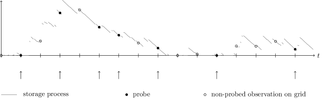
Figure 1: Discrete probing of a storage process. In our model, only the grid observations are observed; the rest of the sample path is merely included for illustration.

Rearranging and taking expectations in the preceding display yields

$$\varphi(\alpha)\,\mathbb{E}e^{-\alpha V_{i}}=\xi\,\mathbb{E}\big{(}e^{-\alpha V_{i}}-e^{-\alpha V_{i-1}}\big{)}+\alpha\,\mathbb{P}(V_{i}=0).$$

The corresponding empirical moment equation is

$$\varphi(\alpha)\frac{1}{n}\sum_{i=1}^{n}e^{-\alpha V_{i}}=\xi\frac{1}{n}\sum_{i=1}^{n}(e^{-\alpha V_{i}}-e^{-\alpha V_{i-1}})+\alpha\frac{1}{n}\sum_{i=1}^{n}\boldsymbol{1}\{V_{i}=0\}.$$

Solving for $\varphi(\alpha)$, and recognizing a telescoping sum, we thus obtain the following estimator for the Lévy exponent $\varphi(\alpha)$:

$$\hat{\varphi}_{n}(\alpha)=\frac{n^{-1}\xi(e^{-\alpha V_{n}}-e^{-\alpha V_{0}})+\alpha n^{-1}\sum_{i=1}^{n}\boldsymbol{1}\{V_{i}=0\}}{n^{-1}\sum_{i=1}^{n}e^{-\alpha V_{i}}}.$$ (7)

Note that this estimator sidesteps the intermediate step of estimating $\psi(\xi)$, which was necessary in the method of Ravner et al., (2019).

The next step is to convert this estimator into an estimator based on observations on the grid $0,\Delta,2\Delta,\ldots,n\Delta$. Such an estimator using the equidistant observations is obtained through discretization. We let

$$S_{i}^{\Delta}=\Delta\left\lfloor S_{i}/\Delta\right\rceil,\qquad V_{i}^{\Delta}=V(S_{i}^{\Delta}),$$

where $\left\lfloor\,\cdot\,\right\rceil$ is the nearest integer function, so that $\Delta\left\lfloor t/\Delta\right\rceil$ is the integer multiple of $\Delta$ closest to any fixed $t\geq 0$. Correspondingly, we define the ‘$\Delta$-counterpart’ of (7):

$$\hat{\varphi}_{n}^{\Delta}(\alpha)=\frac{n^{-1}\xi(e^{-\alpha V_{n}^{\Delta}}-e^{-\alpha V_{0}^{\Delta}})+\alpha n^{-1}\sum_{i=1}^{n}\boldsymbol{1}\{V_{i}^{\Delta}=0\}}{n^{-1}\sum_{i=1}^{n}e^{-\alpha V_{i}^{\Delta}}}.$$ (8)

The factors $n^{-1}$ in (8) are kept since they will be used in the asymptotic analysis later. Note that the observations $V_{i}^{\Delta}$ form a random subset of the equidistant observations $\{V(i\Delta):i=0,1,\ldots\}$. An illustration of this sampling scheme for a given realisation of the workload process is given in Figure 1.

4 Consistency

In this section we prove the following theorem, which states that the estimator $\hat{\varphi}_{n}^{\Delta}(\alpha)$, as constructed in the previous section, is point-wise consistent. In the theorem and its proof, the ‘almost surely’ statements are with respect to any arbitrary initial distribution for $V(0)$. Importantly, the consistency applies regardless the value of the grid width $\Delta.$

Theorem 4.1.

Let $\xi,\Delta>0$ and $\alpha\geq 0$. Then

$$\lim_{n\to\infty}\hat{\varphi}_{n}^{\Delta}(\alpha)=\varphi(\alpha)\text{ a.s.}$$

Proof.

The continuous-time workload process $\{V(t)\}_{t\geq 0}$ is a Harris recurrent Markov process. By Proposition VII.3.8 in Asmussen, (2003), the ‘skeleton process’ $\{V(i\Delta)\}_{i\in\mathbb{N}}$ is a Harris recurrent Markov chain. By a Markov chain ergodic theorem (see e.g. Theorem 14.2.11 in Athreya and Lahiri, (2006)), it thus follows that

$$n^{-1}\sum_{i=1}^{n}f(V(i\Delta))\to\int_{[0,\infty)}f\,\mathrm{d}\pi\text{ a.s.}$$ (9)

for any function $f$ on $[0,\infty)$ integrable with respect to the stationary distribution $\pi$ of $V(\cdot)$. It follows from a pasta-like argument as in Theorem 2 of Makowski et al., (1989) that (9) also holds with $V_{i}^{\Delta}$ replacing $V(i\Delta)$. Taking $f(v)=\boldsymbol{1}\{v=0\}$ and $f(v)=e^{-\alpha v}$ yields

$$\hat{\varphi}_{n}^{\Delta}(\alpha)\to\frac{\alpha\pi(\{0\})}{\displaystyle\int_{[0,\infty)}e^{-\alpha v}\,\pi(\mathrm{d}v)}\text{ a.s.}$$

Now the identities (4) and (5) complete the proof. ∎

5 Central limit theorem

In this section we state and prove a pointwise central limit theorem for the estimation error of $\hat{\varphi}_{n}^{\Delta}$. To do so we consider a high-frequency sampling scheme where the grid width is given by $\Delta=\Delta_{n}=n^{-\gamma}$ for some $\gamma>1/2$. Observe that the total duration of the observation period is then $n\Delta=n^{1-\gamma}$. Therefore, selecting $\gamma<1$ ensures that the process is observed for an increasing period of time as $n$ grows. In the following theorem the specific choice of $\gamma$ is related to the Blumenthal-Getoor index of the process.

We distinguish two cases which we refer to as ‘finite intensity’ and ‘infinite intensity’.

• In the former case the input process $J(\cdot)$ is a compound Poisson process, or equivalently, $\lambda:=\nu(0,\infty)<\infty$. A compound Poisson process can be written as

  $$J(t)=\sum_{i=1}^{N(t)}B_{i},$$

  where $N(\cdot)$ is a Poisson process of rate $\lambda$ and the $B_{i}$ represent i.i.d. jobs with distribution $\lambda^{-1}\nu$.

• In the latter case the input process is not compound Poisson. It is said to have infinite intensity, since its jump measure $\nu$ has infinite mass on the half-line $(0,\infty)$. We distinguish different classes of infinite-intensity jump measures through the Blumenthal-Getoor index

  $$\beta=\inf\left\{b>0:\int_{(0,1)}x^{b}\,\nu(\mathrm{d}x)<\infty\right\}\in[0,1],$$

  originally defined and studied in Blumenthal and Getoor, (1961).

The following result states that our estimator is asymptotically normally distributed, the corresponding variance being expressed in terms of the Lévy exponent (at the target argument $\alpha$ as well as $2\alpha$).

Theorem 5.1.

Suppose that $J(\cdot)$ has Blumenthal-Getoor index $\beta<1/4$, and $\Delta=\Delta_{n}=n^{-\gamma}$ for some $\gamma\in\left(1/(2-2\sqrt{\beta}),1\right)$. Assume that the workload process $V(\cdot)$ is stationary. Then as $n\to\infty$,

$$\sqrt{n}\,(\hat{\varphi}_{n}^{\Delta}(\alpha)-\varphi(\alpha))\rightsquigarrow\mathcal{N}(0,\sigma^{2}),$$ (10)

where $\rightsquigarrow$ denotes weak convergence and

$$\sigma^{2}=\frac{\varphi(\alpha)^{2}}{\alpha\varphi^{\prime}(0)}\Big{(}\alpha+2\xi\Big{(}1-\frac{2\varphi(\alpha)}{\varphi(2\alpha)}\Big{)}+\frac{2\varphi(\alpha)}{\varphi(2\alpha)}(\varphi(\alpha)-\varphi(2\alpha))\Big{)}.$$ (11)

Proof.

Note that by (7),

$$\sqrt{n}(\hat{\varphi}_{n}^{\Delta}(\alpha)-\varphi(\alpha))=\frac{n^{-1/2}\sum_{i=1}^{n}Z_{i}^{\Delta}}{n^{-1}\sum_{i=1}^{n}e^{-\alpha V_{i}^{\Delta}}}$$ (12)

where

$$Z_{i}^{\Delta}=(\xi-\varphi(\alpha))e^{-\alpha V_{i}^{\Delta}}-\xi e^{-\alpha V_{i-1}^{\Delta}}+\alpha\boldsymbol{1}\{V_{i}^{\Delta}=0\}.$$

The proof strategy is to first establish a CLT for the numerator of (12), which is then later used to prove (10). To this end, we approximate $Z_{i}^{\Delta}$ by the counterpart corresponding to the non-truncated observation times,

$$Z_{i}=(\xi-\varphi(\alpha))e^{-\alpha V_{i}}-\xi e^{-\alpha V_{i-1}}+\alpha\boldsymbol{1}\{V_{i}=0\},$$

using the notation of Section 3.

By the identity (6) we have $\mathbb{E}[Z_{i}\,|\,V_{i-1}]=0$, so $Z_{i}$ is a stationary, ergodic martingale difference sequence. A martingale CLT (see e.g. Theorem 18.3 in Billingsley, (1999)) yields, for $\mathbb{E}Z_{1}^{2}\in(0,\infty)$, that

$$n^{-1/2}\sum_{i=1}^{n}Z_{i}\rightsquigarrow\mathcal{N}(0,\mathbb{E}Z_{1}^{2}).$$ (13)

We show at the end of the proof that

$$n^{-1/2}\sum_{i=1}^{n}(Z_{i}^{\Delta}-Z_{i})\rightsquigarrow 0,$$ (14)

so by Slutsky’s Theorem,

$$n^{-1/2}\sum_{i=1}^{n}Z_{i}^{\Delta}=n^{-1/2}\sum_{i=1}^{n}Z_{i}+n^{-1/2}\sum_{i=1}^{n}(Z_{i}^{\Delta}-Z_{i})\rightsquigarrow\mathcal{N}(0,\mathbb{E}Z_{1}^{2}).$$

We will also prove below that

$$n^{-1}\sum_{i=1}^{n}e^{-\alpha V_{i}^{\Delta}}\rightsquigarrow\frac{\alpha\varphi^{\prime}(0)}{\varphi(\alpha)}.$$ (15)

Invoking Slutsky’s Theorem again, it follows that

$$\sqrt{n}(\hat{\varphi}_{n}^{\Delta}(\alpha)-\varphi(\alpha))=\frac{n^{-1/2}\sum_{i=1}^{n}Z_{i}^{\Delta}}{n^{-1}\sum_{i=1}^{n}e^{-\alpha V_{i}^{\Delta}}}\rightsquigarrow\mathcal{N}(0,\sigma^{2}),\qquad\sigma^{2}=\frac{\varphi(\alpha)^{2}\mathbb{E}Z_{1}^{2}}{(\alpha\varphi^{\prime}(0))^{2}}.$$ (16)

Let us first show that the asymptotic variance appearing in (16) is indeed the expression given in (11). Note that by the identity (6),

$$\xi(\xi-\varphi(\alpha))\,\mathbb{E}e^{-\alpha V_{i-1}}e^{-\alpha V_{i}} =\xi\,\mathbb{E}\Big{[}e^{-\alpha V_{i-1}}(\xi-\varphi(\alpha))\mathbb{E}[e^{-\alpha V_{i}}\,|\,V_{i-1}]\Big{]}$$

$$=\xi\,\mathbb{E}\Big{[}e^{-\alpha V_{i-1}}(\xi e^{-\alpha V_{i-1}}-\alpha\mathbb{P}(V_{i}=0\,|\,V_{i-1}))\Big{]}$$

$$=\xi^{2}\,\mathbb{E}e^{-2\alpha V_{i}}-\alpha\xi\,\mathbb{E}e^{-\alpha V_{i-1}}\boldsymbol{1}\{V_{i}=0\}.$$

As a consequence, the variance of $Z_{i}$ can be computed as

$$\mathbb{E}Z_{i}^{2} =((\xi-\varphi(\alpha))^{2}+\xi^{2})\mathbb{E}e^{-2\alpha V_{i}}+(\alpha^{2}+2\alpha(\xi-\varphi(\alpha)))\mathbb{P}(V_{i}=0)$$

$$\phantom{={}}-2\xi(\xi-\varphi(\alpha))\,\mathbb{E}e^{-\alpha V_{i}-\alpha V_{i-1}}-2\alpha\xi\,\mathbb{E}e^{-\alpha V_{i-1}}\boldsymbol{1}\{V_{i}=0\}$$

$$=\Big{(}(\varphi(\alpha)^{2}-2\xi\varphi(\alpha))\frac{2}{\varphi(2\alpha)}+\alpha+2(\xi-\varphi(\alpha))\Big{)}\alpha\varphi^{\prime}(0).$$ (17)

The identity for $\sigma^{2}$ now follows by combining (16) and (17).

It remains to be shown that (14) and (15) hold. We prove (14) by showing that the term in question has vanishing $L^{1}$ norm. Recognizing the telescoping sums noting that $V_{0}^{\Delta}=V_{0}$,

$$\mathbb{E}\Big{|}\sum_{i=1}^{n}e^{-\alpha V_{i}^{\Delta}}-e^{-\alpha V_{i-1}^{\Delta}} -e^{-\alpha V_{i}}+e^{-\alpha V_{i-1}}\Big{|}=\mathbb{E}|e^{-\alpha V_{n}^{\Delta}}-e^{-\alpha V_{n}}|\leq 1,$$

so it follows from the triangle inequality that

$$\mathbb{E}\Big{|}\sum_{i=1}^{n} (Z_{i}^{\Delta}-Z_{i})\Big{|}$$

$$\leq\varphi(\alpha)\sum_{i=1}^{n}\mathbb{E}\big{|}e^{-\alpha V_{i}}-e^{-\alpha V_{i}^{\Delta}}\big{|}+\xi\,\mathbb{E}\Big{|}\sum_{i=1}^{n}e^{-\alpha V_{i}^{\Delta}}-e^{-\alpha V_{i-1}^{\Delta}}-e^{-\alpha V_{i}}+e^{-\alpha V_{i-1}}\Big{|}$$

$$\phantom{={}}+\alpha\sum_{i=1}^{n}\mathbb{E}\big{|}\boldsymbol{1}\{V_{i}^{\Delta}=0\}-\boldsymbol{1}\{V_{i}=0\}\big{|}$$

$$\leq\varphi(\alpha)\sum_{i=1}^{n}\mathbb{E}\big{|}e^{-\alpha V_{i}}-e^{-\alpha V_{i}^{\Delta}}\big{|}+\xi+\alpha\sum_{i=1}^{n}\mathbb{E}\big{|}\boldsymbol{1}\{V_{i}^{\Delta}=0\}-\boldsymbol{1}\{V_{i}=0\}\big{|}.$$

We conclude by showing that both sums in the above display vanish when multiplied by $n^{-1/2}$. Then (14) is a direct consequence, and (15) follows because

$$\mathbb{E}\Big{|}n^{-1}\sum_{i=1}^{n}(e^{-\alpha V_{i}^{\Delta}}-e^{-\alpha V_{i}})\Big{|}\leq n^{-1}\sum_{i=1}^{n}\mathbb{E}|e^{-\alpha V_{i}^{\Delta}}-e^{-\alpha V_{i}}|\to 0,$$

so by Slutsky’s Theorem, the proof of Theorem 4.1, and the identity (4),

$$n^{-1}\sum_{i=1}^{n}e^{-\alpha V_{i}^{\Delta}}=n^{-1}\sum_{i=1}^{n}(e^{-\alpha V_{i}^{\Delta}}-e^{-\alpha V_{i}})+n^{-1}\sum_{i=1}^{n}e^{-\alpha V_{i}}\rightsquigarrow\int e^{-\alpha v}\,\pi(\mathrm{d}v)=\frac{\alpha\varphi^{\prime}(0)}{\varphi(\alpha)}.$$

Here we consider separately the cases of finite and infinite intensity.

$\circ$ Finite intensity case. By conditioning on the number of jobs between $S_{i}$ and $S_{i}^{\Delta}$ and noting that $|S_{i}-S_{i}^{\Delta}|\leq\Delta/2$ it follows that

$$\mathbb{E}|e^{-\alpha V_{i}}-e^{-\alpha V_{i}^{\Delta}}|\leq\int(e^{-\alpha(x-\Delta/2)}-e^{-\alpha x})\,\pi(\mathrm{d}x)+O(\Delta)=O(\Delta).$$

Regarding the other term, note that

$$\mathbb{E}|\boldsymbol{1}\{V_{i}^{\Delta}=0\}-\boldsymbol{1}\{V_{i}=0\}|=\mathbb{P}(V_{i}^{\Delta}=0)+\mathbb{P}(V_{i}=0)-2\,\mathbb{P}(V_{i}^{\Delta}=V_{i}=0).$$

It follows from the stationarity of $V(\cdot)$ that

$$\mathbb{P}(V_{i}^{\Delta}=0)-\mathbb{P}(V_{i}^{\Delta}=V_{i}=0) =\mathbb{P}(V_{i}=0)-\mathbb{P}(V_{i}^{\Delta}=V_{i}=0)$$

$$=(1-\mathbb{P}_{0}(V(|S_{i}^{\Delta}-S_{i}|)=0))\pi(\{0\})$$

$$\leq\mathbb{P}(\text{at least one arrival between }S_{i},S_{i}^{\Delta})=O(\Delta).$$

Both $O(\Delta)$ terms can be bounded by $C\Delta$ for some $C>0$ independent of $i,n$. This means that the $L^{1}$ norm of the remainder term

$$n^{-1/2}\mathbb{E}\Big{|}\sum_{i=1}^{n}(Z_{i}^{\Delta}-Z_{i})\Big{|}$$

can be bounded by a constant times $\Delta\sqrt{n}$. It follows from the assumption that $\Delta=n^{-\gamma}$ for $\gamma>1/2$ that this product vanishes.

$\circ$ Infinite intensity case. Let $\beta_{0}=(\frac{2\gamma-1}{2\gamma})^{2}$, so that $\beta<\beta_{0}<1$, which follows from the assumption on $\gamma$. The following fact, established in the proof of Theorem 3.1 in Blumenthal and Getoor, (1961), will be used later on: given $\delta>\epsilon>\beta$, there exists a positive constant $C$ depending on $\delta$ and $\epsilon$ such that for all sufficiently small $s>0$,

$$\mathbb{P}(J(s)>s^{1/\delta})\leq Cs^{1-\epsilon/\delta}.$$ (18)

Inspecting the proof of the finite-intensity case, it suffices to show that the quantities

$$A(\Delta):=\mathbb{E}|e^{-\alpha V_{i}}-e^{-\alpha V_{i}^{\Delta}}|,\qquad B(\Delta):=1-\mathbb{P}_{0}(V(|S_{i}^{\Delta}-S_{i}|)=0)$$

are both $o(n^{-1/2})$.

Regarding $A(\Delta)$, applying (18) with $\delta=1$ and $\epsilon=\beta_{0}$, we obtain

$$\mathbb{P}(J(s)>s)\leq Cs^{1-\beta_{0}}$$ (19)

so, distributing over the event $\{V(s)>x\}$ and its complement, we find

$$\mathbb{E}_{x}|e^{-\alpha V(s)}-e^{-\alpha x}| \leq\mathbb{P}_{x}(V(s)>x)+\mathbb{E}_{x}(e^{-\alpha V(s)}-e^{-\alpha x})\boldsymbol{1}\{V(s)\leq x\}$$

$$\leq\mathbb{P}(J(s)>s)+\mathbb{E}_{x}\alpha(x-V(s))\boldsymbol{1}\{V(s)\leq x\}$$

$$\leq Cs^{1-\beta_{0}}+\alpha s,$$ (20)

as $s\to 0$, where in the bottom line we use that $V(s)\geq x-s$ given $V(0)=x$. It follows that

$$\int\mathbb{E}_{x}|e^{-\alpha V(s)}-e^{-\alpha x}|\,\pi(\mathrm{d}x)\leq Cs^{1-\beta_{0}}+\alpha s\leq(C+\alpha)s^{1-\beta_{0}}$$

for sufficiently small $s>0$. By conditioning on $\min\{S_{i},S_{i}^{\Delta}\}$ and using that $V(\cdot)$ is a stationary Markov process, it now follows that

$$A(\Delta) =\int\mathbb{E}_{x}|e^{-\alpha V(|S_{i}^{\Delta}-S_{i}|)}-e^{-\alpha x}|\,\pi(\mathrm{d}x)$$

$$\leq(C+\alpha)\mathbb{E}|S_{i}-S_{i}^{\Delta}|^{1-\beta_{0}}$$

$$\leq(C+\alpha)\Delta^{1-\beta_{0}}$$

$$=(C+\alpha)n^{-(4\gamma-1)/(4\gamma)}=o(n^{-1/2}).$$

Regarding the other term $B(\Delta)$, Theorem 2 in Takács, (1966) gives, for $s>0$,

$$1-\mathbb{P}_{0}(V(s)=0) =1-\int_{0}^{s}(1-u/s)\,\mathbb{P}(J(s)\in\mathrm{d}u)$$

$$=\mathbb{P}(J(s)>s)+s^{-1}\int_{0}^{s}u\,\mathbb{P}(J(s)\in\mathrm{d}u)$$

$$\leq Cs^{1-\beta_{0}}+s^{-1}\int_{0}^{s}u\,\mathbb{P}(J(s)\in\mathrm{d}u),$$ (21)

where the last line follows from (19). By (18) with $\delta=\beta_{0}$ and $\epsilon=\beta_{0}^{2}$, we obtain the bound

$$s^{-1}\int_{0}^{s}u\,\mathbb{P}(J(s)\in\mathrm{d}u) =\mathbb{E}s^{-1}J(s)\boldsymbol{1}\{J(s)\leq s^{1/\beta_{0}}\}+\mathbb{E}s^{-1}J(s)\boldsymbol{1}\{s^{1/\beta_{0}}<J(s)\leq s\}$$

$$\leq s^{1/\beta_{0}-1}+\mathbb{P}(J(s)>s^{1/\beta_{0}})$$

$$\leq s^{1/\beta_{0}-1}+Cs^{1-\beta_{0}}$$

(possibly for different $C$ than above) for all $s$ sufficiently small. Since $1-\beta_{0}<1/\beta_{0}-1$, it follows that the dominating term in (21) is of the order $s^{1-\beta_{0}}$, so $B(\Delta)$ is at most of the order $\Delta^{1-\beta_{0}}$, which is $o(n^{-1/2})$ as we already showed. ∎

6 Resampling and a simulation study

We consider an input process $J(\cdot)$ that is the sum of two independent processes $J_{1}(\cdot)$ and $J_{2}(\cdot)$. We take $J_{1}(\cdot)$ to be a Gamma process with shape parameter $\gamma$ and rate parameter $\beta$, meaning that its Lévy exponent is

$$\log\mathbb{E}e^{-\alpha J_{1}(1)}=\int_{0}^{\infty}(e^{-\alpha x}-1)\gamma x^{-1}e^{-\beta x}\,\mathrm{d}x=\gamma\log\frac{\beta}{\beta+\alpha}.$$

It follows that $J_{1}(t)$ has a Gamma$(\gamma t,\beta)$ distribution. We let the second input process $J_{2}(\cdot)$ be an inverse Gaussian process, given by

$$J_{2}(t)=\inf\{s\geq 0:\lambda^{-1/2}W(s)+\mu^{-1}s=t\}$$

for $W(\cdot)$ a standard Brownian motion and $\lambda,\mu>0$ positive constants. Its Lévy exponent is

$$\log\mathbb{E}e^{-\alpha J_{2}(1)}=\int_{(0,\infty)}(e^{-\alpha x}-1)\sqrt{\frac{\lambda}{2\pi}}x^{-3/2}e^{-\lambda x/(2\mu^{2})}\,\mathrm{d}x=\frac{\lambda}{\mu}\left(1-\sqrt{1+2\mu^{2}\alpha/\lambda}\right).$$

The input process $J(t)=J_{1}(t)+J_{2}(t)$ has Lévy density

$$\frac{\mathrm{d}\nu(x)}{\mathrm{d}x}=\gamma x^{-1}e^{-\beta x}+\sqrt{\frac{\lambda}{2\pi}}x^{-3/2}e^{-\lambda x/(2\mu^{2})}.$$

The stability condition is $\gamma/\beta+\mu=\mathbb{E}J(1)<1$, which is fulfilled by our choice $(\gamma,\beta,\mu,\lambda)=(2,5,1,2/5)$.

Simulation can be done by discretizing time and recursively computing the workload through the formula $V(c(i+1))=\max\{0,V(ci)+X(c(i+1))-X(ci)\}$, for some small $c>0$, but the resulting process does not accurately reflect what happens at zero. In particular, the simulated queue is empty much more often than suggested by theory. For us this is very problematic since the estimator of the Lévy exponent relies on these emptiness observations in particular.

We proceed in a different way, estimating the Lévy exponent of $J(\cdot)$ by $\int_{(\epsilon,\infty)}(e^{-\alpha x}-1)\,\nu(\mathrm{d}x)$ for some $\epsilon>0$. This is the exponent of a compound Poisson process

$$J_{\epsilon}(t)=\sum_{i=1}^{N(t)}B_{i},$$ (22)

where $N(\cdot)$ is a time-homogeneous Poisson process of rate $r_{\epsilon}:=\nu(\epsilon,\infty)<\infty$ and the $B_{i}$ are i.i.d. with common distribution $\mathbb{P}(B_{i}\leq x)=r_{\epsilon}^{-1}\nu(\epsilon,x]$. We take $\epsilon=10^{-5}$. We compute numerically the drift of the simulated process

$$\mathbb{E}J_{\epsilon}(1)-1=\int_{(\epsilon,\infty)}x\,\nu(\mathrm{d}x)-1\approx-0.202543$$

which is a reasonable approximation to the true drift $-0.2$.

We simulate the workload process not until a certain number of observations $n$ has been reached, but rather we make the more natural assumptions that the observations $\{V(0),V(\Delta),\ldots,V(T)\}$ are available for some fixed time horizon $T$.

In Figure 4, we show the Lévy exponent $\varphi$ of the process $X(\cdot)$ and its approximation $\varphi_{\epsilon}$ described above. Although the exponents grow apart as $\alpha\to\infty$, the approximation is sufficient for $\alpha\in[0,10]$. We also simulate the reflected process associated with $X_{\epsilon}(t)=J_{\epsilon}(t)-t$ for $t\in[0,25]$ and show $5$ realisations of the estimator $\hat{\varphi}_{n}^{\Delta}$ for the same realisation of the process. The plot shows that the sampling scheme causes much variability in the estimator, when sample sizes are small.

Since Theorem 5.1 prescribes the choice of $\Delta$ as a function of $n$, which is stochastic and unknown a priori, it makes sense to consider the approximation for the time horizon

$$T\approx\mathbb{E}S_{n}^{\Delta}\approx n/\xi.$$

The Blumenthal-Getoor index of the input process $J_{1}(\cdot)+J_{2}(\cdot)$ is $1/2$. Combined with the above approximation and Theorem 5.1 this gives $\Delta\approx(\xi T)^{1/(2-\sqrt{2})}\approx(\xi T)^{-1.707}$. Here we can use the CLT to obtain a confidence interval that is asymptotically valid. A symmetric $95\%$ confidence interval based on the CLT is $\hat{\varphi}_{n}^{\Delta}(\alpha)\pm 1.96\hat{\sigma}/\sqrt{n}$, where $\hat{\sigma}$ is as in $\eqref{e:avar}$ but with $\varphi$ replaced by the estimator $\hat{\varphi}_{n}^{\Delta}$, and $\varphi^{\prime}(0)$ replaced by the estimator $n^{-1}\sum_{i=1}^{n}\boldsymbol{1}\{V_{i}^{\Delta}=0\}$, which was shown to be consistent in the proof of Theorem 4.1. A realisation of the estimator and a region obtained from pointwise confidence intervals is given in Figure 4. For most realisations of the workload process and the estimator, the true parameter $\varphi$ falls nicely within the confidence set.

A resampling procedure

A critical reader may be wondering whether the method proposed here indeed makes efficient use of the available information. Specifically, the workload process is sampled at a discrete collection of time instants, but only a (random) subset of these observations are used in the estimator. This issue is especially important if the sample size is not very large. Therefore, to reduce variance due to the stochastic probing, we now consider the natural assumption that observations of $V(\cdot)$ for the entire grid $\{0,\Delta,\ldots,T\}$ are available, and propose a “resampling” estimator which is the average of $K\in\mathbb{N}$ realisations $\hat{\varphi}_{k,n(k)}^{\Delta}$ of the original estimator

$$\hat{\varphi}_{\text{r},K}^{\Delta}:=\frac{1}{K}\sum_{k=1}^{K}\hat{\varphi}_{k,n(k)}^{\Delta},$$

where $n(k)$ is the number of probes in iteration $k$. Recall that for a given grid the number of observations sampled for the approximate estimator is a random variable, hence it may vary between iterations. Taking $K$ large enough will “exhaust the information” in the sample of workload observations on the grid, and reduce the aforementioned variability. In practice, $K$ can be chosen by simulation since $\hat{\varphi}_{\text{r},K}^{\Delta}$ can be computed fast (given a sample, one computes the estimator a few times and checks if it does not vary too much).

Figure 4 shows two realisations of $\hat{\varphi}_{\text{r},K}^{\Delta}$ each for three values of $\Delta$, again all based on the same simulated workload process. Per value of $\Delta$, the pairs of realisations are close, illustrating that the variance due to the random sampling is reduced significantly by applying the resampling procedure. It varies across simulations of the workload process for which value of $\Delta$ the estimator is closest to the true $\varphi$, but variations are mostly due to the stochastic nature of the workload process. In general taking smaller $\Delta$ is best, for it reduces bias and variance.

Figure 2: 5 realisations of $\hat{\varphi}_{n}^{\Delta}$ using $\xi=\Delta=1$, based on a simulated workload process observed for $t\in[0,25]$, whose input is $J_{\epsilon}$ defined in (22). On the right, in grey, are the number of probes $n$ for each realisation.

Figure 3: Estimator and approximate pointwise confidence intervals based on the Central Limit Theorem using $\xi=1$ and $\Delta=4\cdot 10^{-4}\approx 100^{-1.707}$, based on a simulated workload process observed for $t\in[0,100]$, whose input $J_{\epsilon}$ is defined in (22).

Figure 4: Realisations of $\hat{\varphi}_{\text{r},K}^{\Delta}$ using $\xi=1$ and $K=1000$, for various $\Delta$, based on a simulated workload process observed for $t\in[0,25]$, whose input is $J_{\epsilon}$ defined in (22). The grey numbers on the right indicate the value of $\Delta$.

7 Conclusion

This paper has introduced an estimator of the Lévy exponent for the subordinator input to a Lévy-driven queue given equidistant observations of the workload. For any grid width $\Delta$ the estimator is consistent. Asymptotic normality of the estimation errors is further derived for a high-frequency sampling regime where $\Delta$ decreases at an appropiate rate as the sample size grows. Establishing a low-frequency central limit theorem for a fixed $\Delta$ is an open challenge. As the estimator is strongly consistent, we know that the bias term in the estimation equation vanishes as the sample size grows. However, there is no guarantee that this holds for the variance term as well. On the contrary, we conjecture that $\Delta$ should appear in the asymptotic variance term, but this requires a different proof strategy than that used in Theorem 5.1. This framework can potentially be applied for non-parametric estimation of the Lévy measure itself by applying an inversion formula (see Abate and Whitt, (1992)). Again, such analysis requires careful treatment of the distribution of the estimation error due to the discrete approximation of the moment equation.

A resampling scheme was further suggested that constructs the approximate moment estimation equation for many randomly selected sub-samples on the discrete grid. The rationale behind this procedure is that in any single iteration some of the available data is discarded in the estimation process. Simulation analysis suggests that this scheme indeed reduces the variance of the estimation error, but no theoretical guarantees are provided. Establishing such results is also an interesting open challenge that requires ad-hoc treatment of the underlying dependence structure of the workload process.

References

- Abate and Whitt, (1992) Abate, J. and Whitt, W. (1992). The Fourier-series method for inverting transforms of probability distributions. Queueing systems, 10(1):5–87.
- Asanjarani et al., (2021) Asanjarani, A., Nazarathy, Y., and Taylor, P. (2021). A survey of parameter and state estimation in queues. Queueing Systems, 97(1):39–80.
- Asmussen, (2003) Asmussen, S. (2003). Applied Probability and Queues. Springer-Verlag.
- Athreya and Lahiri, (2006) Athreya, K. B. and Lahiri, S. N. (2006). Measure Theory and Probability Theory. Springer-Verlag.
- Baccelli et al., (2009) Baccelli, F., Kauffmann, B., and Veitch, D. (2009). Inverse problems in queueing theory and internet probing. Queueing Systems, 3(63):59–107.
- Basawa et al., (1996) Basawa, I., Narayan Bhat, U., and Lund, R. (1996). Maximum likelihood estimation for single server queues from waiting time data. Queueing Systems, 24(1-4):155–167.
- Belomestny and Reiß, (2015) Belomestny, D. and Reiß, M. (2015). Estimation and calibration of Lévy models via Fourier methods. In Lévy Matters IV, pages 1–76. Springer.
- Billingsley, (1999) Billingsley, P. (1999). Convergence of Probability Measures. John Wiley & Sons.
- Bingham and Pitts, (1999) Bingham, N. H. and Pitts, S. M. (1999). Non-parametric estimation for the M/G/ queue. Annals of the Institute of Statistical Mathematics, 51(1):71–97.
- Blumenthal and Getoor, (1961) Blumenthal, R. M. and Getoor, R. K. (1961). Sample functions of stochastic processes with stationary independent increments. Journal of Mathematics and Mechanics, 10(3):493–516.
- Dębicki and Mandjes, (2015) Dębicki, K. and Mandjes, M. (2015). Queues and Lévy fluctuation theory. Springer.
- Goldenshluger, (2016) Goldenshluger, A. (2016). Nonparametric estimation of the service time distribution in the M/G/ queue. Advances in Applied Probability, 48(4):1117–1138.
- Hansen and Pitts, (2006) Hansen, M. and Pitts, S. (2006). Nonparametric inference from the M/G/1 workload. Bernoulli, 12(4):737–759.
- Kappus and Reiß, (2010) Kappus, J. and Reiß, M. (2010). Estimation of the characteristics of a Lévy process observed at arbitrary frequency. Statistica Neerlandica, 64(3):314–328.
- Kella et al., (2006) Kella, O., Boxma, O., and Mandjes, M. (2006). A Lévy process reflected at a Poisson age process. Journal of Applied Probability, 43(1):221–230.
- Makowski et al., (1989) Makowski, A., Melamed, B., and Whitt, W. (1989). On averages seen by arrivals in discrete time. In Proceedings of the 28th IEEE Conference on Decision and Control, pages 1084–1086.
- Mandjes and Ravner, (2021) Mandjes, M. and Ravner, L. (2021). Hypothesis testing for a Lévy-driven storage system by Poisson sampling. Stochastic Processes and their Applications, 133:41–73.
- Prabhu, (1998) Prabhu, N. (1998). Stochastic Storage Processes. Springer-Verlag.
- Ravner et al., (2019) Ravner, L., Boxma, O., and Mandjes, M. (2019). Estimating the input of a Lévy-driven queue by Poisson sampling of the workload process. Bernoulli, 25(4B):3734–3761.
- Takács, (1966) Takács, L. (1966). The distribution of the content of a dam when the input process has stationary independent increments. Journal of Mathematics and Mechanics, 15(1):101–112.
- van Es et al., (2007) van Es, B., Gugushvili, S., and Spreij, P. (2007). A kernel type nonparametric density estimator for decompounding. Bernoulli, 13(3):672–694.